


Abstract
Accurate evaluation of the Strouhal number is important for wind-resistant design, but traditional aerodynamic assessments are computationally expensive. To support rapid schematic design, this paper proposes a deep learning framework to predict the Strouhal number for 2D bluff bodies. Arbitrary irregular sections are represented using a unified three-channel geometric tensor that combines distance and spatial coordinate fields. A Residual Network integrated with Coordinate Attention, termed ResCA-Net, is developed to focus on vortex-shedding determinants, particularly leading-edge separation points. The model was trained on 1000 randomly generated convex sections, with target St values obtained from 2D URANS simulations at Re = 2 × 10⁴. On an independent test set, ResCA-Net achieves an R2 of 0.9129, an MAE of 0.0316, and a median absolute percentage error of 6.56%. Systematic benchmarking shows that the embedded Coordinate Attention outperforms SE, CBAM, and the baseline ResNet. A single inference takes only 43.56 milliseconds, which is over 160,000 times faster than transient CFD simulations. This end-to-end method provides an efficient and accurate surrogate model for rapid iterative screening of aerodynamic shapes.
1. Introduction
Slender structures such as high-rise buildings and long-span bridges are highly susceptible to flow-induced vibrations (FIV) under wind actions, including flutter and vortex-induced vibration (VIV). The collapse of the Tacoma Narrows Bridge in 1940 due to wind-induced flutter has become a landmark case in structural wind engineering [1]. Similarly, in 2021, the SEG Plaza in Shenzhen experienced perceptible vibrations, which were attributed to vortex-induced vibration of the building’s rooftop mast [2]. These classical cases from civil engineering illustrate the fundamental physical mechanism: when the vortex shedding frequency approaches the natural frequency of a structure, resonant vibration can occur, leading to severe damage or serviceability issues.
Beyond civil infrastructure, the same vortex-induced vibration mechanism poses significant challenges in aerospace engineering. The Strouhal number (St), which characterizes the vortex shedding frequency, serves as a critical parameter for predicting such resonant risks. In aircraft design, the prediction of vortex shedding frequency is essential for assessing vibration and fatigue in landing gear systems, where flow past bluff-body components such as struts and wheel assemblies has been identified as a source of structural vibration during takeoff and landing configurations [3]. In unmanned aerial vehicle design, the wake interference and vortex shedding from bluff-body components such as arms and fuselage segments can affect flight stability and structural integrity. In engine nacelle design, the interaction between the nacelle and the surrounding flow can generate periodic vortex shedding that excites structural modes and contributes to noise and vibration. These examples highlight that rapid and accurate prediction of the vortex shedding frequency is broadly relevant across both civil and aerospace engineering contexts.
As highlighted by these diverse engineering challenges, the Strouhal number is of central interest in flow-induced vibration studies because it governs the fundamental lock-in mechanism between vortex shedding and structural motion [4]. As summarized in the comprehensive review on bluff-body VIV, the synchronization of shedding frequency with structural natural frequency, which is uniquely determined by the Strouhal number, is the essence of flow-induced resonant vibrations. In engineering practice, the Strouhal number serves as a critical first-level screening metric for VIV risk assessment during the schematic design phase. For instance, experimental studies on bridge deck torsional VIV have demonstrated that the Strouhal number provides a direct quantitative link between cross-sectional geometry and vibration susceptibility [5]. Therefore, predicting the Strouhal number is not merely an intermediate step in aeroelastic analysis, but an essential front-end tool for identifying high-risk geometries and prioritizing candidate sections for more detailed evaluations, thereby avoiding costly late-stage design modifications. Furthermore, the Strouhal number is intrinsically linked to vortex-induced vibration and flow separation, which are the two key phenomena governing the aerodynamic stability of bluff bodies. Flow separation at geometric discontinuities generates periodic vortex shedding, and the separated shear layer directly determines the shedding frequency. This physical mechanism underscores why the Strouhal number is both physically meaningful and practically valuable for rapid aerodynamic assessment. In the schematic phase of wind-resistant structural design, if the St corresponding to the 2D cross-sectional shape of a slender structure can be rapidly obtained, designers can assess VIV risks early and optimize cross-sectional parameters. However, given the diverse cross-sectional shapes in engineering, traditional methods struggle to efficiently and cost-effectively meet the evaluation demands for a massive number of candidate 2D sections. Therefore, there is an urgent need to develop a high-precision and flexible method for the rapid prediction of the Strouhal number.
Traditional approaches for obtaining the Strouhal number primarily include wind tunnel tests, field measurements, and computational fluid dynamics (CFD) simulations. Although wind tunnel tests offer high accuracy, they suffer from long cycles and high costs; any modification to the cross-sectional shape or flow conditions necessitates a new set of experiments, making it difficult to accommodate the rapid iterations required during the design phase [6]. Field measurements can only be conducted post-construction, rendering them incapable of serving the preliminary design phase, and are further hindered by complex environments and implementation difficulties [7,8]. CFD simulations balance cost and flexibility to some extent; however, high-fidelity unsteady flow analysis of a 2D section for a single case often still takes hours to days [9,10]. The common bottleneck of these traditional methods is that when evaluating the Strouhal number for a multitude of different cross-sectional shapes, the time and computational costs become prohibitive, severely constraining the efficiency of aerodynamic shape optimization.
In recent years, machine learning (ML) methods have demonstrated immense potential in aerodynamic shape recognition and aerodynamic parameter prediction. Early studies predominantly utilized Backpropagation Neural Networks (BPNNs), validating the feasibility of neural networks in this field. Li et al. [11] and Li et al. [12] developed BPNN models taking the geometric shape and angle of attack of girder sections as inputs to predict the static three-component aerodynamic coefficients. Similarly, Jung et al. [13] employed BPNNs to estimate the aeroelastic parameters of bridge decks, while Chen et al. [14] utilized artificial neural networks to predict flutter derivatives, collectively demonstrating that neural networks are capable of capturing complex dynamic aeroelastic behaviors. Huang [15] further applied BPNNs to predict the flutter critical wind speed and static aerodynamic coefficients of flat box girders and inverted trapezoidal box girders. These studies indicate that even relatively simple neural networks can mine meaningful mapping relationships from aerodynamic shapes. With deeper investigations, scholars have begun to explore more diverse model architectures and shape representation methods. For the same prediction task, Liao et al. [16] systematically compared the performance of four ML algorithms, namely Support Vector Regression (SVR), Neural Networks (NN), Random Forest Regression (RFR), and Gradient Boosting Regression Tree (GBRT), using geometric information and dynamic parameters as inputs, revealing the pros and cons of different algorithms. Hu et al. [17,18] evaluated Decision Tree Regressors, Random Forests, and GBRTs for predicting the wind pressure around a 2D smooth cylinder, selecting the GBRT as the optimal model. Regarding shape representation, Chen et al. [19] proposed a novel conditional Generative Adversarial Network that utilized a binary matrix to represent aerodynamic shapes, enhancing both flexibility and accuracy. Miyanawala et al. [20] applied the Euclidean distance field as the input for a Convolutional Neural Network (CNN) to establish the functional relationship between bluff body shape parameters and the three-component aerodynamic forces, successfully predicting lift and drag coefficients. Beyond force coefficient regression, recent deep learning studies have also demonstrated remarkable capabilities in reconstructing full flow fields and serving as CFD surrogates. Bhatnagar et al. [21] employed a CNN architecture to map the pixelated geometry representation of airfoils using a signed distance function directly to the full velocity and pressure fields, achieving predictions four orders of magnitude faster than conventional numerical solvers. To further enhance the mapping accuracy for complex flow fields, Thuerey et al. [22] systematically investigated deep learning models based on the U-Net architecture. Their work highlighted the critical importance of network architecture design, specifically the integration of residual and skip connections, in effectively capturing shape-to-flow mappings, thereby achieving highly accurate predictions on previously unseen shapes. Building upon this framework, recent advanced deep learning models have further strengthened the capability of direct shape-to-parameter mapping. For example, Seo et al. [23] utilized CNNs to accurately predict the force coefficients of cylinders subjected to complex geometric disturbances. Furthermore, to replace computationally expensive CFD simulations, Liu et al. [24] developed a deep neural network as a robust surrogate model, successfully predicting the aerodynamic coefficients of parameterized cross-sections within a second. Recently, physics-informed neural networks have emerged as an alternative paradigm that incorporates governing equations as soft constraints [25]. In contrast to this approach, our method is purely data-driven and achieves superior inference speed for rapid screening tasks. The aforementioned studies fully demonstrate that ML can effectively extract complex mappings between aerodynamic shapes and parameters, with extremely fast prediction speeds post-training, providing a feasible pathway for the rapid acquisition of St. However, existing works still exhibit two notable limitations. First, most studies target static aerodynamic coefficients or flutter critical wind speed, paying insufficient attention to St, which reflects the periodic dynamic behavior of vortex shedding. The nonlinear mapping relationship between St and cross-sectional morphology is highly complex, demanding superior dynamic feature extraction capabilities from the models. Second, the majority of methods rely on parameterized geometric descriptions or prior assumptions of specific cross-sectional forms. Traditional parameterization approaches such as Bézier curves, B-splines, or class-shape transformation typically assume that cross-sections belong to specific predefined families, including rectangular, trapezoidal, or streamlined box girders. Notably, many existing machine learning studies in this field have been confined to specific geometric families, including circular and rectangular cylinders [20], parametrized airfoil sections [24], and cylinders with wavy disturbances [23], limiting their applicability to diverse arbitrary convex cross-sectional shapes encountered in engineering practice.
To address these issues, this paper proposes a deep learning model named ResCA-Net, which integrates a Residual Network (ResNet) with a Coordinate Attention (CA) mechanism, establishing an end-to-end intelligent prediction method mapping from 2D bluff body aerodynamic shapes to the Strouhal number. Its effectiveness is validated on a dataset of unsteady flows past 1000 randomly generated 2D bluff body sections. Given that the proposed method targets a screening-level prediction with an inference time of 43.56 ms per sample, its primary value lies in enabling high-frequency iterative assessments during the early design phase, where absolute precision may be traded for speed to explore a broader design space. The core innovations of this paper are manifested in three aspects: (1) At the input feature level, a consistent shape representation combining a distance field and coordinate fields is introduced. This enables the model to uniformly process various irregular convex sections, eliminating the prior dependency of traditional parameterized methods on specific cross-sectional forms. (2) At the network architecture level, ResNet is fused with the CA mechanism. Through shallow attention for spatial anchoring and deep attention focusing on the leading-edge separation point, the model is guided to adaptively capture the geometric features dictating the vortex shedding frequency. We systematically benchmark this mechanism against mainstream alternatives, namely Squeeze-and-Excitation and Convolutional Block Attention Module, to demonstrate its superiority in aerodynamic shape recognition tasks. (3) At the prediction target level, addressing the fact that St is more unsteady and highly nonlinear than traditional static force coefficients, the feasibility of deep learning methods in predicting such dynamic aerodynamic parameters is validated, achieving significant computational acceleration while maintaining high accuracy. This paper aims to provide efficient and low-cost technical support for the rapid acquisition of St and aerodynamic shape optimization in structural wind-resistant design.
The remainder of this paper is organized as follows: Section 2 introduces the construction pipeline of the unsteady flow dataset based on 2D URANS and proposes the consistent feature representation method for irregular sections. Section 3 constructs the ResCA-Net prediction architecture integrating residual structures and cross-stage Coordinate Attention (CA). Section 4 systematically validates the effectiveness and physical interpretability of the model through multi-dimensional accuracy evaluation, ablation experiments, and flow field visualization. Section 5 summarizes the main conclusions and outlines future work.
2. Dataset Construction
2.1. Data Generation
This study employs computational fluid dynamics (CFD) simulations to generate the dataset required for neural network training. The numerical simulations are conducted using a self-developed 2D CFD platform, which has been validated in previous studies [26,27]. The research focuses on irregular convex bluff body sections, whose geometries are generated via a random point generation algorithm. Specifically, the Graham scan algorithm is applied in conjunction with geometric operations such as polar angle sorting, distance calculation, and cross-product determination, to construct the initial convex hull polygons. Subsequently, normalization is applied to ensure that the characteristic width B of all sections is exactly 1.0, while the height is randomly scaled within the range of 0.3 to 1.0 and centrally aligned. This procedure is repeated to generate 1000 distinct geometries of irregular convex bluff body sections.
As illustrated in Figure 1, a rectangular computational domain is utilized. The length and width of the domain are dynamically generated by the program, both strictly exceeding 30 times the total section width (30B), to ensure the full development of the flow field. A no-slip boundary condition is applied to the structural walls, where both normal and tangential velocities are set to zero. A velocity inlet boundary condition is adopted with an inflow velocity of U = 1 m/s and a reference static pressure of 0. A pressure outlet boundary condition is set at the exit, where variables such as velocity and pressure are treated with a zero-gradient condition. Slip boundary conditions are imposed on the top and bottom boundaries, ensuring zero normal velocity while allowing free tangential velocity. The fluid density is set to ρ = 1.225 kg/m3. Although the dynamic viscosity μ = 6.125 × 10⁻⁵ Pa · s is higher than that of air under standard conditions, it was chosen for numerical convenience to achieve the target Reynolds number of Re = 2.0 × 10⁴; with U = 1 m/s and B = 1 m, thereby avoiding fractional velocity or length scales. This Reynolds number was selected because it lies in the typical subcritical regime, where vortex shedding is well-established and stable, making it ideal for systematic data generation. Since the Reynolds number alone determines the flow regime, the non-physical viscosity does not alter the essential flow physics. To guarantee that the flow reaches a statistically stationary state, a flow field recorder is configured to calculate the time-averaged flow field starting from a designated moment, saving the flow state for subsequent post-processing.
Figure 1.
Schematic diagram of the 2D computational domain.
To accommodate the generated complex geometric boundaries, the computational model employs highly adaptable unstructured meshes for spatial discretization, with local refinements applied in the near-wall region to accurately capture boundary layer characteristics and shear layer separation. The flow solver is based on the 2D Finite Volume Method (FVM), utilizing the incompressible Unsteady Reynolds-Averaged Navier–Stokes (URANS) equations coupled with the k − ω SST turbulence model for unsteady computations. The key numerical parameters are summarized in Table 1.
Table 1.
Key numerical parameters of the CFD simulation.
The reliability of the present CFD framework is established through rigorous validation in previous studies that employed the identical numerical platform. Fang et al. [26] used the same 2D CFD platform to simulate the vortex-induced vibration (VIV) of a semi-open twin-box deck and directly compared their CFD results with rigid-body sectional model wind tunnel tests. Their comparison demonstrated favorable agreement in the lock-in region and maximum vibration amplitude, confirming that the CFD platform can reliably reproduce the essential flow physics of bluff-body vortex shedding. Liu et al. [27] further conducted a systematic mesh independence study on the same platform, computing the aerostatic drag coefficient using four distinct mesh densities and comparing the results with wind tunnel measurements. The simulation error converged from 26.52% with the coarsest mesh to just 2.48% with the finest mesh, demonstrating that the platform achieves grid-converged solutions with sufficient mesh resolution. Based on classical reviews on bluff-body vortex shedding [4], a tolerance of 5% is commonly accepted for Strouhal number validation. We adopt this 5% tolerance as the benchmark for our dataset generation.
To ensure consistent accuracy across the 1000+ random geometries in the present dataset, an automated meshing algorithm with uniform topology-adaptive refinement was strictly enforced. Following the same mesh generation strategy and expansion ratios (e.g., progressive size increment factor) as those employed in the validated studies, the base mesh size was configured to align with the converged settings reported by Liu et al. [27]. Consequently, the total element count adapts dynamically to the geometric complexity of each polygon (typically ranging from 150,000 to 300,000 elements), ensuring consistently sufficient spatial resolution while controlling computational cost.
It is worth noting that the present study required the generation of a large-scale dataset comprising over 1000 unsteady CFD cases to support the training of the deep learning model. Given this substantial computational demand, the validated 2D URANS framework represents the optimal balance between computational efficiency and physical accuracy for dataset generation. The 2D approximation is justified for slender structures where the cross-sectional geometry varies slowly along the spanwise direction, such as long-span bridge decks, high-rise buildings, and aerospace components with bluff-body features (e.g., landing gear struts, engine nacelles, UAV arms). This approximation is widely adopted in the wind engineering and aerodynamics communities. For cases with significant spanwise variations, three-dimensional simulations would be required; however, the present 2D framework serves as a computationally efficient and physically reliable baseline for cross-sectional aerodynamic characterization.
2.2. Input Feature Design
2.2.1. Consistent Representation Method
This study aims to establish an end-to-end prediction model mapping arbitrary irregular bluff body sections to their corresponding Strouhal numbers. To prevent the deep learning model from developing inaccurate understandings of complex geometric features, a unified representation method for arbitrary sections is imperative. Drawing inspiration from the consistent shape representation method proposed by Li et al. [28], this paper computes an exact Euclidean distance field and orthogonal spatial coordinate fields. Combined with pseudo-color encoding techniques, the geometric information of the sections is mapped into a combination of high-dimensional image features, achieving a unified description of the aerodynamic shapes of arbitrary bluff body sections.
While pseudo-color encoding does not introduce new physical variables beyond the original scalar fields, it plays a critical role in facilitating deep representation learning. As demonstrated in previous studies on aerodynamic shape representation using CNNs [20,28], standard convolutional kernels are inherently sensitive to high-contrast edges and spatial gradients. Pseudo-color mapping acts as a non-linear contrast enhancement mechanism, transforming smooth scalar transitions into distinct visual boundaries. This optimized inductive bias significantly aids the shallow convolutional layers in explicitly locking onto topological discontinuities, such as bluff-body corners and potential separation points, thereby accelerating convergence and improving ultimate predictive capacity compared to processing raw, low-contrast scalar arrays. We also acknowledge that the performance gain could partly be attributed to increased model capacity, and a systematic comparison between scalar and pseudo-color inputs is left for future work.
Based on the exact Euclidean distance transform, the distance field function is defined as:
where Ddist is the normalized distance field value of a spatial point P; d(P, ∂Ω) is the shortest Euclidean distance from the spatial point to the external boundary of the aerodynamic section ∂Ω; and max(d) is the maximum distance within the computational domain. This formulation ensures that regions closer to the boundary possess values closer to 1.
The streamwise (horizontal) coordinate field function is defined as:
where X is the horizontal pixel coordinate of a spatial point, and Xcenter is the coordinate of the horizontal centerline of the flow field. This function characterizes the relative streamwise position from the pixel to the section center via linear attenuation.
The crosswind (vertical) coordinate field function is defined as:
where Y is the vertical pixel coordinate, and Ycenter is the coordinate of the vertical centerline.
As illustrated in Figure 2, to further enhance the convolutional neural network’s capacity to extract local features, the Jet pseudo-color mapping algorithm is employed to convert the aforementioned three single-channel scalar fields (normalized to [0, 1]) into RGB three-channel color images. Taking the distance field as an example, it maps spatial proximity through color variations (values closer to 1 appear dark red, while values closer to 0 appear dark blue), visually reinforcing the boundary information. The coordinate fields depict central symmetry and gradient variations in the streamwise and crosswind directions, respectively. After being expanded via pseudo-color mapping, the three feature fields collectively construct an information-rich, multi-channel shape representation.
Figure 2.
Examples of consistent representation of aerodynamic shapes.
2.2.2. Input Data Generation Pipeline
Upon completing the CFD computations for the 1000 sections, the geometric shape of each section must be converted into the standard input format for the neural network, while the corresponding Strouhal number is extracted as the output label. The overall pipeline is as follows:
- Geometric Shape Imaging and Tensor ConstructionFor each section, its binary contour is first extracted, followed by high-resolution interpolation and edge detection. Subsequently, the distance field, streamwise coordinate field, and crosswind coordinate field are calculated according to the formulas in Section 2.2.1. Each field is independently converted into a 224 × 224 × 3 RGB image utilizing Jet pseudo-color mapping. Finally, the RGB images of the three fields are concatenated along the channel dimension, expanding the original geometric contour into a 9-channel feature tensor. This results in a standardized dataset with dimensions of ( 1000 , 224 , 224 , 9 ), which serves as the input for ResCA-Net.
- Flow Field Post-processing and St ExtractionFor the CFD results of each section, the time history of the lift coefficient CL is extracted. The time window after the flow is fully developed (t = 150 s to 300 s) is isolated. A Fast Fourier Transform (FFT) is performed on the mean-subtracted CL sequence (to remove any non-zero mean due to geometric asymmetry, as illustrated in Section 4.3.5) to identify the dominant vortex shedding frequency f. The Strouhal number is calculated by:
All input tensors were verified to be free of NaN or infinite values, and the value range of each channel was confirmed to lie within [0, 1]. The statistical distributions of the input features were also checked to be consistent across the training, validation, and test sets. The aforementioned pipeline ensures a deterministic mapping relationship between the inputs (geometric images) and the outputs (St), providing a standardized dataset for the subsequent neural network training. The dataset and the ResCA-Net source code are provided as Supplementary Materials.
2.3. Dataset Statistics and Splitting
2.3.1. Sample Scale and Geometric Diversity
A total of 1000 irregular convex bluff body section samples were generated in this study. To ensure dataset diversity, sufficient constraints were applied to the geometric morphology during the generation process: the characteristic width of all samples was uniformly normalized, the height was randomly scaled within a specified range, and the randomness of the section contours was guaranteed by the random point generation algorithm. Figure 2 displays the geometric morphologies of several representative sections, encompassing typical categories such as near-rectangular sections, sharp-edged sections, and highly asymmetric sections, which reflects the dataset’s coverage capacity for complex aerodynamic shapes.
To further quantify the geometric diversity of the dataset, the geometric characteristics of all samples were statistically analyzed. The aspect ratio ranges from 1.00 to 3.33; the convex hull perimeter ranges from 2.09 to 3.76; and the section area is distributed between 0.004 and 0.877. These metrics cover a broad spectrum of geometric shapes, ranging from flat to towering, and from compact to slender. Figure 3 presents the histogram of the Strouhal number distribution. The values are predominantly concentrated in the range of 0.2 to 0.5, which aligns with classic empirical values for vortex shedding frequencies in bluff body aerodynamics. Concurrently, a small number of samples deviate from this interval; these correspond to specific aerodynamic shapes featuring sharp edges, drastic local concave–convex variations, or strong asymmetries. These outlier samples serve as critical training materials for the model to learn complex nonlinear mappings. Statistical analysis reveals that the minimum and maximum St across all samples are 0.0067 and 1.00, respectively, with a mean of 0.308 and a standard deviation of 0.163. The data distribution effectively spans the spectrum from low to high vortex shedding frequencies.
Figure 3.
Histogram of Strouhal number distribution.
2.3.2. Dataset Splitting
Given that all section samples were independently and randomly generated, with their geometric morphologies following the same distribution, this study employs a simple random sampling method for dataset splitting. Initially, all samples are randomly shuffled, and then divided into a training set, a validation set, and an independent test set at a ratio of 8:1:1. Specifically, the training set contains 800 samples used for model parameter optimization, the validation set comprises 100 samples utilized for hyperparameter tuning and early stopping decisions, and the test set contains 100 samples used exclusively for the final performance evaluation. The test set was kept completely unseen during model development. The validation and test sets adequately cover the full distribution ranges of aspect ratio, section area, and Strouhal number, enabling an effective assessment of the model’s generalization capabilities.
3. Network Model
3.1. Overall Network Architecture
The ResCA-Net model is designed to achieve an end-to-end nonlinear mapping from aerodynamic shape images to the Strouhal number (St). The overall network architecture, illustrated in Figure 4, employs an improved ResNet-34 as the backbone feature extractor. The input to the model is the consistently represented 9-channel spatial feature tensor with dimensions of (224 × 224 × 9). We chose 224 × 224 pixels because it is the standard input size for classic CNN architectures such as ResNet-34. It provides sufficient spatial resolution to capture fine geometric features such as sharp corners and edge curvatures, while maintaining computational efficiency.
Figure 4.
Overall network architecture of the ResCA-Net model. In the diagram, light blue blocks represent residual blocks, orange blocks indicate coordinate attention modules, and grey blocks denote standard operations (e.g., initial stem, pooling, and fully connected layers).
The input tensor first undergoes preliminary feature extraction and spatial downsampling through an initial block (Stem), which contains a 7 × 7 convolution (stride of 2) and max pooling. Subsequently, the feature maps sequentially flow through four residual stages (ResBlock 1 to 4, primarily composed of stacked 3 × 3 convolutional layers). As the network deepens, the spatial resolution of the feature maps is halved at each stage, while the number of channels is doubled. To enhance the model’s spatial perception of critical physical regions, Coordinate Attention (CA) modules are embedded after ResBlock 2 and ResBlock 4, respectively. The final high-dimensional feature maps are compressed into a 1D vector via Global Average Pooling (GAP), and a fully connected layer outputs the final predicted St value.
3.2. Residual Module
The Strouhal number (St) is highly sensitive to the geometric details of the section, necessitating the network to possess multi-level representation capabilities ranging from local edges to global contours. Given the highly nonlinear nature of this mapping, traditional deep networks are prone to gradient degradation. To address this, this study employs residual modules as the fundamental units for geometric feature extraction, as illustrated in Figure 5. When the input and output dimensions are identical, an identity mapping residual block is used, as shown in Figure 5a, which losslessly transmits preceding features via skip connections. When the channel or spatial dimensions of the feature map change, a projection mapping residual block is applied, as depicted in Figure 5b, utilizing a 1 × 1 convolution to adjust dimensions to match the addition operation. This design effectively mitigates the optimization difficulty in deep networks, ensuring that foundational geometric boundary information is not lost while extracting abstract, high-order physical semantics.
Figure 5.
Structures of basic residual modules: (a) Identity mapping residual block; (b) projection mapping residual block. Solid arrows indicate the direction of data flow, while dashed lines point to visual representations of intermediate features. Regarding the colored blocks, grey represents convolutional and dropout layers, orange indicates batch normalization, and light blue denotes ReLU activation layers.
Both identity and projection residual blocks use the same ReLU activation function (f(x) = max(0, x)). The only difference is that the projection block employs a 1 × 1 convolution to match dimensions when the input and output channels differ, while the identity block passes the input directly via skip connections.
3.3. Coordinate Attention Mechanism
In flow field prediction tasks, the model must accurately localize key regions such as leading-edge separation points and curvature variations on the windward face. However, the 2D global pooling operation in traditional channel attention inevitably discards spatial coordinate information. Therefore, this paper introduces the Coordinate Attention (CA) mechanism, as shown in Figure 6. This mechanism factorizes the attention into 1D feature encodings along both horizontal and vertical directions. Through aggregation in these orthogonal directions, the CA module explicitly embeds spatial positional information into the attention weights while establishing cross-channel dependencies. This guides the model to adaptively focus on critical coordinate points that govern the vortex shedding frequency, while simultaneously suppressing background noise.
Figure 6.
Structure of the Coordinate Attention (CA) mechanism.
Coordinate attention decomposes channel attention into two one-dimensional feature encoding processes, which respectively aggregate features along the horizontal (width direction) and vertical (height direction) spatial directions. For the input feature map X ∈ R^(C × H × W), coordinate attention first performs average pooling along the horizontal and vertical directions, obtaining feature encodings in these two directions. Subsequently, these two encodings are concatenated and input into a shared 1 × 1 convolution transformation, and then split along the spatial dimension into two independent tensors. These tensors are respectively processed by a 1 × 1 convolution and a sigmoid function to generate the attention weights gh and gw for the horizontal and vertical directions. Finally, the output feature map is the element-wise product of the input and the two attention weights:
Y = X⊙gh⊙gw
3.4. ResCA-Net Hybrid Architecture
In Convolutional Neural Networks, as the depth increases, the spatial resolution of feature maps decreases while semantic information strengthens. For aerodynamic shape recognition, the Strouhal number is governed not only by macroscopic features like the overall blockage width but is also highly sensitive to local geometric details such as leading-edge separation points and sharp corners. To balance global and local features, instead of the conventional practice of densely stacking attention modules in every layer, this study selectively embeds CA modules at the outputs of ResBlock 2 and ResBlock 4, constructing a cross-stage collaborative feature extraction architecture.
The rationale behind this design is that feature maps at different depths possess entirely distinct receptive fields and informational emphases. The shallower ResBlock 2 outputs feature maps of 28 × 28, retaining abundant spatial details and geometric boundary information. The primary objective of embedding the first attention module at this stage is to conduct a preliminary screening of effective geometric regions in the flow field at a macroscopic scale. Since the input image contains a large area of uniform flow field background, the shallow attention mechanism utilizes coordinate information to prioritize network weights on the windward contour and the wake boundary on the leeward side of the section. This operation effectively suppresses useless background noise in the early stages of feature extraction, providing a clear macroscopic blockage candidate region for subsequent layers.
As the network deepens, the feature map dimension output by ResBlock 4 drops to 7 × 7 after multiple downsampling operations. At this stage, although the features encapsulate highly abstract fluid dynamics semantics, the pooling operations inevitably weaken the model’s precise perception of spatial coordinates. Embedding a second attention module in this deeper stage primarily serves to compensate for the loss of critical positional information. Building upon the noise filtering achieved in the shallow layers, the deep attention mechanism can further refine localization within the narrow feature space. It converges the focus onto microscopic local regions that dominate the vortex shedding frequency, such as abrupt geometry changes at the leading edge. This enables the network to accurately extract the core physical points that dictate flow separation.
Overall, embedding attention modules in both shallow and deep layers forms a “coarse-to-fine” feature focusing mechanism. The shallow module is responsible for locking onto macroscopic blockage boundaries, while the deep module refines microscopic separation points; the two complement each other in both spatial scale and physical semantics. Compared to merely increasing the depth of the backbone network, this collaborative design effectively alleviates the loss of local geometric details in deep networks while introducing negligible computational burden (with a parameter increase of less than 0.5%). Furthermore, it aligns the model’s feature extraction process more closely with the physical principles transitioning from overall flow blockage to local shear layer separation.
3.5. Model Training Strategy
The proposed model is constructed based on the TensorFlow deep learning framework and Keras API, and trained on an NVIDIA RTX 3060 GPU (NVIDIA Corporation, Santa Clara, CA, USA). To ensure stable convergence and prevent overfitting on a finite-scale dataset, the Adaptive Moment Estimation (Adam) optimizer is employed to update the network weights, coupled with an L2 regularization mechanism. Mean Squared Error (MSE) is adopted as the loss function.
During the training process, an appropriate batch size is set considering GPU memory constraints and the smoothness of gradient updates. Regarding learning rate scheduling, a dynamic decay strategy based on validation loss (ReduceLROnPlateau) is introduced, which adaptively reduces the learning rate when the validation loss fails to exhibit a downward trend over specific epochs. Furthermore, to capture the model weights with the best generalization capability, an Early Stopping mechanism is configured to terminate training prematurely if the validation loss shows no improvement within the defined patience threshold. The specific key hyperparameter configurations for model training are summarized in Table 2.
Table 2.
Key hyperparameter configurations for model training.
4. Results and Discussion
4.1. Comparative Experiments
The comparative experiments in Section 4.1 and Section 4.2 are conducted on the validation set (800/200 split) for model selection and hyperparameter tuning. The independent test set (800/100/100 split) is used exclusively for the final evaluation in Section 4.3.
4.1.1. Loss Function Comparison
In regression prediction tasks, the selection of the loss function significantly influences the optimization trajectory and the ultimate generalization performance of deep learning models. To determine the optimal objective function, this study compared Mean Squared Error (MSE), Mean Absolute Error (MAE), and Huber loss under identical hyperparameter configurations. Figure 7 presents the global convergence curves of the Validation Root Mean Square Error (RMSE) on a logarithmic scale for the three loss functions, along with locally magnified details during the late training stage.
Figure 7.
Training and validation loss convergence curves under different loss functions.
Huber loss combines the advantages of MSE (smooth gradients near zero) and MAE (robustness to outliers). However, in our experiments, Huber performed between MSE and MAE, indicating that the dataset does not contain enough extreme outliers to benefit from Huber’s robust properties. In the early training stage (Epoch < 20), MSE exhibits larger oscillations than MAE and Huber. This is because the quadratic penalty of MSE generates stronger gradients for large errors, which helps the network escape initial local minima. MAE, with its constant gradient magnitude, lacks this capability.
As training progresses to the middle and late stages (Epoch > 60), the quadratic property of MSE allows its gradients to adaptively decay with the error, enabling precise local optimization near the optimal solution. In contrast, MAE and Huber exhibit higher convergence lower bounds due to their constant gradients or piecewise penalty strategies. Quantitative results in the legend reveal that MSE ultimately achieves the lowest steady-state validation error (RMSE = 0.0274) with minimal fluctuation (±0.0040), significantly outperforming Huber (0.0374 ± 0.0081) and MAE (0.0559 ± 0.0114). Comprehensive consideration of these dynamic characteristics and convergence accuracy justifies the selection of MSE as the loss function for the network.
4.1.2. Backbone Network Comparison
To identify the optimal foundational feature extractor, this study compared residual networks of varying depths while keeping the proposed Coordinate Attention (CA) module fixed. The results are summarized in Table 3. The analysis indicates that ResNet-18, due to its shallower architecture, possesses a restricted receptive field and limited nonlinear representational capacity, leading to relatively high error metrics. Conversely, when the network depth increases to ResNet-50, slight overfitting occurs due to the constraints of the current dataset scale, which paradoxically degrades the prediction accuracy on the validation set. Balancing model capacity, prediction accuracy (R2 = 0.9757), and computational resource overhead, ResNet-34 achieves the optimal equilibrium for this task and is therefore designated as the baseline backbone network.
Table 3.
Comparative experiments of different backbone networks.
4.1.3. Attention Mechanism Comparison
To verify the superiority of Coordinate Attention (CA) in aerodynamic shape recognition tasks, it was benchmarked against the mainstream Squeeze-and-Excitation (SE) and Convolutional Block Attention Module (CBAM). The visualized heatmaps are detailed in Figure 8, and the corresponding evaluation results are presented in Figure 9.
Figure 8.
Heatmap comparison of different attention mechanisms. The solid white outlines superimposed on the heatmaps denote the geometric boundaries of the input aerodynamic cross-sections.
Figure 9.
Comprehensive performance radar chart of different attention mechanisms.
As observed in the top row of Figure 8, the SE module produces a diffuse response primarily clustered at the center of the cross-sections. It is important to note that SE, by design, acts as a purely channel-wise attention mechanism. Through global average pooling, it compresses spatial dimensions to recalibrate channel weights, which is typically sufficient and highly effective for general image classification where global features dominate. However, aerodynamic evaluation presents a unique physical challenge: the influence of local geometric topology on flow characteristics exhibits nonlinear amplification (e.g., minute modifications to a leading-edge corner can drastically alter flow separation behavior). Therefore, relying solely on the global features extracted by SE is inadequate.
While CBAM (middle row of Figure 8) incorporates spatial attention to address this, its activation regions still exhibit significant background noise and scattered focus, likely due to the absence of explicit directional coordinate encoding. In contrast, benefiting from precise positional encoding along orthogonal directions, the heatmaps generated by the proposed CA mechanism (bottom row of Figure 8) display a clear, structured spatial distribution. CA accurately covers the windward leading edges and forms pronounced spatial activation peaks precisely at the critical geometric mutations. For Sample 1 (near-polygonal section with sharp leading edges), CA produces significantly higher activation than CBAM because CBAM’s spatial attention lacks explicit directional encoding, causing it to miss the sharp corners that dominate flow separation. The explicit directional encoding of CA provides the network with spatial sensitivity analogous to capturing local boundary layer separation points in CFD, which explains its superior performance for Sample 1.
The introduction of CA is therefore not merely an algorithmic enhancement, but a physics-informed architecture design dictated by the inherent physical sensitivity of aerodynamic shapes.
To quantitatively and intuitively evaluate the performance enhancements brought by different attention mechanisms, Table 4 summarizes the raw evaluation metrics, and Figure 9 illustrates a comprehensive performance radar chart. The evaluation encompasses six dimensions: coefficient of determination (R2), error metrics (1-RMSE and 1-MAE), training stability (Stability), training smoothness (Smoothness), and convergence efficiency (LossDropRate). The six metrics in Figure 9 are transformed to a comparable [0, 1] scale, where 1 indicates the best performance. R2 is used directly. The 1-RMSE and 1-MAE are computed as clip(1 − error/0.1, 0.5, 1.0), where the reference value 0.1 is chosen based on the typical magnitude of errors in this task. Stability is defined as 1/(1 + 3 × CV), where CV is the coefficient of variation of the validation loss over the last 10 epochs. Smoothness is defined as 1/(1 + 5 × V), where V is the mean absolute difference of consecutive training losses. LossDropRate is the relative reduction from the initial to the final training loss, clipped to [0.5, 1.0]. Numerical ticks are provided at each concentric level of the radar chart.
Table 4.
Quantitative performance evaluation of different models.
As depicted by the red contour in Figure 9, the proposed ResCA-Net covers the largest area on the radar chart, forming the outermost envelope across the core predictive and stability dimensions. Quantitative data from Table 4 further corroborates this visual dominance. ResCA-Net achieves the highest R2 (0.9757), significantly outperforming the baseline ResNet (0.9125), CBAM (0.9599), and SE (0.9583). Furthermore, it provides the most robust error control with an RMSE of 0.0253 and MAE of 0.0182, while its global stability score (0.9401) vastly exceeds the SE module (0.7678). Although CBAM and the baseline show marginally higher Smoothness and LossDropRate respectively, ResCA-Net comprehensively yields the optimal balance for high-precision aerodynamic predictions. Notably, LossDropRate measures the relative training loss reduction; ResCA-Net achieves approximately 0.84 (an 84% drop). This metric is primarily used for relative comparison across models rather than as an absolute measure of quality.
4.2. Ablation Study
4.2.1. Model Component Ablation
Using ResCA-Net (the complete model) as the baseline, the coordinate attention module and the residual modules were systematically removed to establish four comparative configurations: (1) complete model (ResNet-CA, comprising both residual and coordinate attention modules); (2) removal of coordinate attention (Standard ResNet, retaining only residual modules); (3) removal of residual modules (pure convolutional network embedded with coordinate attention, denoted as CNN-CA); and (4) removal of both (pure convolutional network, denoted as CNN). By horizontally comparing the performance of these configurations, the necessity of both module types and their synergistic effects are revealed.
Figure 10 illustrates the comparison of performance on the validation set and model complexity among the four configurations. Starting from the complete model (ResNet-CA), removing the coordinate attention (ResNet) causes the RMSE to increase from 0.0253 to 0.0473, and the R2 to drop from 0.976 to 0.913, with a negligible parameter reduction of approximately 0.1 M (from 21.8 M to 21.7 M). This significant decline in accuracy indicates that coordinate attention effectively guides the model to focus on leading-edge separation points by encoding positional information along horizontal and vertical directions. This drop directly reflects the vital contribution of the CA module to the extraction of spatially sensitive features.
Figure 10.
Comparison of model performance metrics and parameter counts across ablation configurations.
When residual modules are removed (CNN-CA), the RMSE rises to 0.0630 and R2 drops to 0.823, despite a 3 M increase in parameters. This confirms that residual skip connections are essential for reaching sufficient depth to extract multi-level geometric features. When both components are removed (CNN), performance drops to RMSE = 0.0827 and R2 = 0.724. Notably, the magnitude of this decline manifests as a nonlinear compounding effect, and the nonlinear compounding effect between residual connections and coordinate attention means that their combined benefit exceeds the sum of their individual contributions. The residual network provides deep feature extraction capability, while coordinate attention performs precise spatial calibration upon this foundation. In practice, this synergy enables the model to achieve higher accuracy with fewer parameters than naive stacking of attention modules, making it more suitable for deployment in resource-constrained environments.
4.2.2. Parametric Analysis
To investigate the optimal spatial embedding strategy for the Coordinate Attention (CA) module, this section utilizes the standard ResNet without attention mechanisms as the baseline model. Four differentiated CA module configurations were designed: shallow-to-middle layers (Block 1&3), deep layers (Block 3&4), all layers (All Blocks), and intermittent embedding (Block 2&4, the strategy ultimately adopted in this paper). The quantitative comparison results are presented in Figure 11. The findings indicate that the model’s predictive performance does not improve monotonically with the number of stacked attention modules; instead, it exhibits significant spatial sensitivity to the embedding locations.
Figure 11.
Grouped bar chart of attention position ablation.
The proposed “Block 2&4” combination achieves the optimal performance (RMSE = 0.025, R2 = 0.976). In contrast, improper positioning or excessive stacking degrades representational efficiency. The “Block 3&4” strategy bypasses mid-level spatial constraints, leaving the deep-layer attention without sufficient positional priors, resulting in a slight RMSE increase to 0.029. Embedding across all blocks (All Blocks) leads to feature redundancy due to overly frequent nonlinear reassignments, which to some extent interferes with the identity mapping transmission of the residual network, similarly elevating the RMSE to 0.029. Furthermore, introducing attention prematurely in extremely shallow layers (Block 1&3, RMSE = 0.047) causes the mechanism to erroneously amplify high-frequency noise in the background, resulting in performance degradation. Overall, the “Block 2&4” strategy circumvents the aforementioned issues while securing substantial spatial perception gains with a marginal increase in parameters.
4.2.3. Ablation on Input Representations
To validate the superiority of the proposed distance-field-based geometric tensor, an ablation experiment was conducted comparing it against a standard Signed Distance Function (SDF) representation. A 3-channel SDF input was constructed and fed into the same ResCA-Net architecture. Evaluated on the independent test set, the SDF-based model achieved an R2 of 0.794 and an MAE of 0.0504, exhibiting a noticeable performance drop compared to the proposed encoding strategy (R2 = 0.9129, MAE = 0.0316).
From an aerodynamic perspective, this discrepancy is highly interpretable. While SDF excellently captures the purely local geometric morphology, it inherently lacks global spatial context. The Strouhal number is not only dependent on the shape but is extremely sensitive to the object’s orientation relative to the incoming flow. The proposed encoding strategy explicitly embeds the streamwise and crosswind coordinate fields, providing the network with a crucial global frame of reference. This allows the attention mechanisms to accurately distinguish between the windward flow-blocking surface and the leeward wake region, proving the necessity of the proposed multi-channel geometric formulation.
4.3. Model Performance Evaluation
4.3.1. Prediction Accuracy Analysis
The predictive performance of the proposed ResCA-Net model was evaluated on an independent test set comprising 100 samples. To ensure absolute fairness in architectural comparisons (Section 4.1), the model was tested under an independent inference phase. By loading the optimal weights corresponding to the lowest validation loss and enforcing the strict evaluation mode (e.g., disabling Dropout), the model achieved its best performance.
As depicted in the scatter plot in Figure 12, the vast majority of the predicted samples converge tightly along the ideal y = x diagonal line, with an inference RMSE of 0.0410. A linear regression analysis of the prediction distribution yields a global trendline equation of y = 0.8711x + 0.0576. The fact that the slope closely approximates 1 and the intercept approaches 0 rigorously demonstrates, from a statistical perspective, that the model exhibits no systematic overestimation or underestimation bias within the global parameter space.
Figure 12.
Scatter plot of predicted versus actual values on the independent test set.
Regarding the RMSE of 0.0410, while this absolute value might initially appear notable given the small typical magnitude of the Strouhal number (St), it is crucial to evaluate this metric within the context of the dataset’s variance. Therefore, we introduce the Normalized Root Mean Square Error (NRMSE). In the current study, the distribution range of St across diverse aerodynamic shapes is approximately 0.9933 (Range = Stmax − Stmin ≈ 1 − 0.0067 = 0.9933). Consequently, the NRMSE is calculated as follows:
Coupled with a high coefficient of determination (R2) of 0.9129, a Mean Absolute Error (MAE) of 0.0316, and a Median Absolute Percentage Error (MdAPE) of 6.56%, this low NRMSE indicates that the deep learning predictions are in good agreement with the high-fidelity CFD ground truth. It should be noted that the Mean Absolute Percentage Error (MAPE) is 16.86%, which appears higher than the MdAPE. This is because a few samples with relatively low St values produce larger percentage errors due to the small denominator. The MdAPE, which is robust to such outliers, is only 6.56%. Further analysis of the error distribution indicates that 36.0% of the samples possess an absolute percentage error of less than 5%, and 63.0% of the samples possess an absolute percentage error of less than 10%. The maximum absolute error, which occurs under a specific extreme geometric section condition, is 0.1382, remaining well within acceptable engineering tolerances.
To provide a direct comparison with our model, a Random Forest regressor was also evaluated on the same independent test set. It achieved an R2 of 0.484 and an MAE of 0.0765, which is significantly lower than the proposed ResCA-Net (R2 = 0.9129, MAE = 0.0316). This large performance gap confirms that conventional tree-based models cannot capture the complex spatial features required for accurate Strouhal number prediction, and that the proposed deep learning architecture is necessary for this task.
Regarding the distribution pattern, the majority of the direct CFD calculation results cluster around St ≈ 0.2. This is consistent with empirical values for classical vortex shedding frequencies in bluff body aerodynamics, indicating that the core of the dataset possesses robust physical validity. Notably, a minority of samples exhibit calculation results that deviate significantly from this constant range. Even so, the model maintains robust prediction stability for these extreme conditions. This fully illustrates that the model has not only learned the universal mapping relationship between the flow field and the Strouhal number but also possesses the capability to capture complex nonlinear features within the geometric parameter space covered by the dataset. Future work will test the model on unseen shape families to further assess its transferability.
4.3.2. Error Distribution Analysis
To further quantify the statistical characteristics of the prediction errors, Figure 13 presents a comprehensive residual analysis on the independent test set, comprising three complementary views: residual distribution, quantile–quantile (Q-Q) plot, and cumulative error distribution.
Figure 13.
Residual analysis results on the independent test set. (a) Residual distribution histogram with a Gaussian fit; (b) Quantile-Quantile (Q-Q) plot of the ordered values against theoretical quantiles, the blue circles represent the ordered quantiles of the actual residuals, while the solid red line indicates the reference for a theoretical normal distribution.; (c) Cumulative probability curve of the absolute prediction error.
As shown in Figure 13a, the residual distribution histogram is generally symmetrically distributed around a near-zero mean, and the overall prediction residuals follow a highly concentrated Gaussian distribution (μ = 0.0213, σ = 0.0350), with the absolute residual values of most samples being less than 0.10. Furthermore, the Q-Q plot in Figure 13b indicates that the residuals approximately follow a normal distribution. Although the small positive mean (μ = 0.0213) indicates a very slight systematic shift, this bias remains minimal and well within an acceptable range. Finally, the cumulative error distribution curve in Figure 13c shows that 90% of the samples have an absolute error of less than 0.0681. This verifies that, following the introduction of the coordinate attention mechanism, the model effectively overcomes the nonlinear perturbations introduced by extreme aerodynamic shapes and possesses outstanding global robustness.
To assess the acceptability of the prediction errors, we compare our results with recent machine learning studies on aerodynamic parameter prediction. Hu and Kwok [17] applied machine learning techniques to predict wind pressures around circular cylinders and reported that well-trained models achieve R2 values typically in the range of 0.85 to 0.95. Miyanawala and Jaiman [20] reported that CNN-based models for lift and drag coefficient prediction achieve errors of approximately 5% to 10%. In our study, the model achieves an R2 of 0.9129 and an MAE of 0.0316 on the independent test set. The corresponding median absolute percentage error (MdAPE) is 6.56%, indicating that the majority of samples are predicted within 6.56% relative error. These error levels are within the range reported in the literature and are acceptable for screening-level prediction in the preliminary design phase.
4.3.3. Computational Efficiency Analysis
Compared to traditional CFD simulations, the proposed model demonstrates a profound efficiency advantage. For a single aerodynamic parameter evaluation, the single-step inference based on an NVIDIA RTX 3060 GPU (NVIDIA Corporation, Santa Clara, CA, USA) requires only 43.56 milliseconds; in contrast, completing a URANS transient simulation of equivalent accuracy typically takes 2 h (7200 s). The model achieves an acceleration factor exceeding 160,000, successfully transforming computationally exhaustive simulation tasks into model inferences executable on a single consumer-grade GPU. While the training data generation cost is approximately 2000 GPU hours (1000 CFD cases × 2 hours each) and model training takes approximately 4 h on the same GPU, these are one-time costs. Once trained, each inference takes only 43.56 ms, enabling rapid screening of thousands of candidate sections at negligible marginal cost. This provides an extremely cost-effective and feasible solution for high-frequency evaluations required in large-scale parametric scanning of sections and wind-resistant optimization design.
4.3.4. Visualization Analysis
To further investigate the sensitivity of the model to geometric features at different hierarchical levels, Figure 14 selects three representative cross-sections (Sample 1: a near-polygonal section; Sample 2: a sharp-edged section; and Sample 3: a highly asymmetric section) to display the heatmap responses generated by the shallow and deep Coordinate Attention (CA) mechanisms.
Figure 14.
Comparison of shallow and deep attention heatmaps. In the heatmaps, the solid white outlines represent the geometric boundaries of the input aerodynamic cross-sections. In the top row, the red outlines highlight regions where the shallow layers capture the global geometric contours and windward edges. In the bottom row, the red circles indicate localized regions of high activation in the deep layers, specifically pointing to critical geometric mutations such as sharp leading edges.
In the shallow network (top row, Block 2), the high-response regions (warm-colored areas) do not uniformly cover all geometric boundaries; instead, they exhibit strong directional selectivity. The attention weights are scattered along the macroscopic windward contours and the boundary trends of the initial wake zones. This indicates that the shallow layers primarily extract low-level, macroscopic geometric boundary information. Conversely, in the deep network (bottom row, Block 4), as the semantic features are condensed, the attention weights exhibit intense local convergence. The high-response regions rapidly contract from the macroscopic contours and focus highly near the sharp corners of the windward leading edge.
Further observation of the different morphologies reveals: For Sample 1, the deep layer accurately anchors the windward corner points at the leading edge. For Sample 2, the strongest activation directly locks onto the prominent windward tip. For Sample 3, the deep layer stably locates and focuses on the dominant geometric extremity.
The geometric sensitivity of the Strouhal number is rooted in the fact that local geometric features control the location of flow separation, which in turn determines the vortex shedding frequency and VIV characteristics. This mechanism is well supported by both CFD analysis and experimental evidence. Fang et al. [26] demonstrated that for semi-open twin-box decks, the upstream maintenance railings, despite being small-scale features relative to the overall deck dimensions, generated a separation bubble that evolved into large-scale vortices and directly determined the shedding frequency and VIV amplitude. Liu et al. [27] further showed that in central-slotted box girders, the aerodynamic forces on specific surface regions made dominant contributions to the vortex-excited force, with the leading-edge regions of the downstream box exhibiting the strongest correlation with the overall VEF. These findings confirm that leading-edge separation points and sharp corners are the critical geometric features controlling flow separation and vortex shedding. In our study, the attention heatmaps in Figure 14 are fully consistent with these physical findings: the deep layer concentrates on the leading-edge regions where flow separation initiates, while the shallow layer encodes the macroscopic geometry. This alignment indicates that the model has learned to identify the same geometric features that physically determine the Strouhal number and VIV susceptibility, providing a physically grounded explanation for the high sensitivity of St to sectional geometry. This not only verifies the effectiveness of the synergistic architecture designed in Section 3.4 from a feature-extraction perspective but also provides robust, physics-aligned interpretability for the internal decision-making logic of the deep neural network.
4.3.5. Time-Frequency Characteristic Analysis
The accurate prediction of the Strouhal number depends fundamentally on the precise capture of the transient dynamics within the flow field. Figure 15 presents the lift coefficient time-history curves (top row) and their corresponding Power Spectral Density (PSD) analyses (bottom row) obtained from numerical CFD simulations for three representative sections: a near-rectangular section (Sample 1), a sharp-edged section (Sample 2), and a highly asymmetric section (Sample 3).
Figure 15.
Comparison of lift coefficient time-history curves and power spectral density (PSD) analyses for three representative sections.
The vortex shedding frequency (St) is directly related to the unsteady shear stress on the body surface. Higher shedding frequencies induce more rapid fluctuations in the wall shear stress, which in turn affects the mean and fluctuating aerodynamic forces. This relationship is particularly important for fatigue analysis of slender structures, where high-frequency vortex shedding can excite structural modes and accelerate damage accumulation. Significant variations are observed in the lift oscillation periods and spectral peaks across sections with diverse morphologies. Sample 1 is a near-rectangular section, which typically exhibits well-defined, nearly sinusoidal vortex shedding characteristics. In contrast, Sample 3 is a highly asymmetric section where the vortex shedding is significantly perturbed by the geometry, leading to more complex lift coefficient time histories. This is consistent with the findings of Liu et al. [27], who showed that aerodynamic forces during VIV exhibit significant variations depending on the geometric configuration. The variation in lift coefficient characteristics across different geometries is the fundamental physical basis for our geometry-to-Strouhal-number prediction task. It is worth noting that the frequency resolution of the FFT is limited by the fixed temporal window of 150 s, yielding Δf = 1/150 ≈ 0.0067 Hz. For low-frequency shedding (St < 0.1), the number of cycles captured within this window is relatively small, which can lead to less sharp spectral peaks and may contribute to slightly larger errors for these samples. This is an inherent limitation of the fixed-window spectral analysis. Nevertheless, the proposed model maintains robust prediction stability for these low-frequency cases, demonstrating its capability to capture the dominant frequency even when the spectral peak is less pronounced.
Despite the high complexity of the underlying flow field structures and wake shedding modes, the predicted St values output by the proposed model (represented by the blue dash-dotted lines in Figure 15) accurately align with the dominant frequency peaks derived from the rigorous CFD calculations (represented by the red dashed lines). Specifically, for Samples 1 and 2, the predicted peaks (0.447 and 0.194) nearly perfectly coincide with the CFD ground truths (0.439 and 0.195). Even for the highly asymmetric Sample 3, where flow separation is exceptionally complex, the prediction (0.213) tightly tracks the primary CFD peak (0.195) with acceptable engineering deviation.
From a physical perspective, this precise spectral alignment decisively demonstrates that the deep learning model has not degenerated into mere numerical curve-fitting. Rather, guided by the aforementioned attention mechanisms, it has genuinely captured the nonlinear dynamic essence of the flow field structures that physically dictate the vortex shedding frequencies.
4.3.6. Comparative Discussion
To further validate the proposed ResCA-Net and highlight its unique contributions, this section benchmarks the present findings against recent deep learning studies in the field of bluff-body aerodynamics. The superiority of the current framework is demonstrated in three primary aspects.
- Geometric Generality for Arbitrary SectionsMost recent machine learning frameworks in wind engineering rely on geometric parameterization. For example, Miyanawala and Jaiman [20] predicted forces on circular and rectangular cylinders, but their model was constrained by the specific shapes. Seo et al. [23] utilized deep learning for cylinders with wavy disturbances, and Liu et al. [24] focused on parameterized airfoil sections. Viquerat et al. [29] developed a supervised neural network for drag prediction of arbitrary 2D shapes, but their study was limited to laminar flow conditions. While these studies achieved high accuracy within their defined domains, they cannot generalize beyond predefined topologies or flow regimes. In contrast, the present study introduces a universal distance-field-based geometric tensor. By training on over 1000 completely random, non-parameterized convex polygons, our model breaks topological barriers, enabling direct predictions for arbitrary convex bluff-body shapes that do not conform to standard parametric equations under turbulent flow conditions.
- Physical Interpretability of Attention MechanismsDeep learning in fluid mechanics is frequently criticized for its lack of interpretability. Recent assessments of supervised machine learning methods for fluid flows have highlighted that these models often function as black boxes, providing accurate predictions without revealing the underlying physical mechanisms Fukami et al. [30]. The present study addresses this limitation by embedding the Coordinate Attention mechanism. As discussed in Section 4.3 and visualized in the feature heatmaps of Figure 14, our network does not merely memorize data; it actively learns to focus on the geometric discontinuities at the leading-edge windward side. This neural activation coincides with the physical location of shear layer separation, which is the fundamental driver of vortex shedding. This high degree of physical interpretability represents a significant advancement over conventional data-driven models.
- Computational Efficiency of Distance-Field RepresentationRecently, Graph Neural Networks have gained popularity for handling arbitrary geometries, as they can process non-uniform, unstructured fluid meshes Pfaff et al. [31]. However, representing fluid domains as graphs requires the explicit construction of massive node-and-edge adjacency matrices. The continuous message-passing across hundreds of thousands of nodes incurs significant computational overhead, memory bottlenecks, and latency during inference. The proposed method bypasses this bottleneck entirely. By transforming arbitrary polygons into distance-field geometric tensors, we map irregular shapes onto a highly regular, structured Cartesian grid. This allows us to leverage highly optimized, matrix-based operations inherent to modern CNN architectures rather than graph algorithms. Consequently, our approach eliminates the need for unstructured graph generation, drastically reducing memory consumption while achieving millisecond-level Strouhal number predictions. This computational agility makes the current framework exceptionally suited for massive shape-screening tasks in preliminary engineering design.
5. Conclusions and Future Work
This paper proposes a deep learning methodology integrating a residual network with a cross-stage coordinate attention mechanism (ResCA-Net), establishing an end-to-end intelligent prediction architecture from the unified aerodynamic shape of irregular bluff body sections to the Strouhal number (St). The primary research conclusions are as follows:
- Unified encoding of arbitrary convex sections.Traditional parameterization methods can only handle predefined shape families, such as specific airfoils or rectangular cylinders. In this work, the proposed three-channel distance-field tensor converts any convex polygon into a structured image-like representation. This removes the need for manual feature design and allows the model to process a wide range of irregular cross-sections without retraining or shape-specific adjustments.
- Physical interpretability through hierarchical attention.Ablation studies and visualization analyses demonstrate that the proposed Block 2 and Block 4 dual-node CA mechanism is effective. The network does not act as a black box. Instead, it shows a coarse-to-fine focusing pattern: the shallow attention captures overall flow-blocking boundaries, while the deep attention concentrates on leading-edge shear layer separation points. This indicates that ResCA-Net learns physically meaningful features related to vortex shedding, improving the interpretability of deep learning models in fluid mechanics.
- Accurate prediction on arbitrary shapes.On an independent test set of random geometries, the model achieves an R2 of 0.9129, an MAE of 0.0316, and a median absolute percentage error of 6.56%. Systematic benchmarking confirms that the embedded Coordinate Attention outperforms mainstream mechanisms such as SE and CBAM, as well as the baseline ResNet. This level of accuracy provides a reliable quantitative basis for aerodynamic parameter prediction in preliminary design.
- High computational efficiency for large-scale screening.By mapping unstructured geometries onto structured Cartesian grids, the proposed framework avoids the computational overhead of traditional CFD and complex Graph Neural Networks. The trained model requires only 43.56 milliseconds for a single inference, which is over 160,000 times faster than 2D transient CFD simulations. This makes ResCA-Net suitable for rapid aerodynamic screening and shape optimization in structural wind engineering.
The proposed method has potential applications in several practical scenarios. It can enable rapid screening of aerodynamic cross-sections for UAV wings and arms during conceptual design, where quick St estimates are needed for flutter risk assessment. It is also applicable to landing gear door design, where complex bluff-body flows are encountered and iterative CFD is computationally prohibitive. Furthermore, it can support real-time shape optimization loops where traditional CFD is infeasible due to time constraints. Beyond these, the unified shape representation that combines distance and coordinate fields allows the model to cover a diverse geometric space that is not limited to predefined shape families. This space includes irregular struts, asymmetric support structures, simplified landing gear door profiles, and novel bridge deck sections, provided they are convex polygons. The model is developed for two-dimensional flow at a constant subcritical Reynolds number of 20,000, and it achieves a screening-level prediction accuracy with an R2 of 0.9129, an RMSE of 0.0410, an MAE of 0.0316, and a median absolute percentage error of 6.56%. Although this error level may not replace high-fidelity CFD simulations for final design certification, it is highly valuable for the early conceptual design phase, where downstream tasks such as generative aerodynamic design or structural optimization of UAV components often require evaluating thousands of candidate cross-sections and absolute precision can be traded for evaluation speed. With an inference time of only 43.56 ms per sample, which is over 160,000 times faster than transient CFD simulation, ResCA-Net acts as an ultra-fast aerodynamic filter. It enables designers to rapidly assess the vortex shedding characteristics of thousands of irregular shapes and reliably eliminate those prone to severe flow-induced vibration or resonance. The promising candidates that survive this screening can then be passed to expensive CFD simulations or wind tunnel tests. Therefore, the current error level and design space meet the demands of high-frequency iterative assessment and significantly accelerate the early-stage design process.
The current model validation is primarily established under the ideal conditions of a fixed subcritical Reynolds number (Re = 2 × 10⁴) and non-concave sections. Oriented towards actual engineering environments, future work can be expanded in two dimensions. Firstly, by augmenting the morphological diversity of the dataset to include concave sections and real bridge sections with complex ancillary structures (e.g., railings, fairings), thereby further validating and enhancing the model’s topological generalization capability. Secondly, inspired by the recent advancements demonstrated by Lin et al. [25] in applying physics-informed deep learning to two-dimensional bluff body aerodynamics, exploring the integration of physics-informed neural network paradigms (such as PINNs) to incorporate critical physical parameters (e.g., Reynolds number) and governing equations as input variables or loss functions represents a crucial path toward enhancing the model’s physical interpretability and generalization ability. Unlike the purely data-driven approach presented in this work, PINNs offer a complementary framework that embeds physical laws directly into the learning process, which could be particularly valuable when training data are scarce or when extrapolation to unseen flow regimes is required.
Supplementary Materials
The following supporting information can be downloaded at https://doi.org/10.5281/zenodo.22909795 (accessed on 21 September 2026). Dataset S1: Complete dataset and code for “Intelligent Prediction of Aerodynamic Parameters for Flow Past 2D Bluff Body Sections at a Constant Reynolds Number” (including geometric feature tensors, Strouhal number labels, and ResCA-Net source code).
Author Contributions
Conceptualization, Q.K., K.L. and L.M.; methodology, Q.K. and L.M.; software, Q.K., B.Y. and S.L.; validation, Q.K., B.Y. and Y.Q.; formal analysis, Q.K., L.M. and S.L.; investigation, Q.K. and Y.Q.; resources, K.L. and L.M.; data curation, Q.K. and B.Y.; writing—original draft preparation, Q.K. and L.M.; writing—review and editing, Q.K., K.L. and L.M.; visualization, Q.K.; supervision, K.L.; project administration, K.L.; funding acquisition, L.M. All authors have read and agreed to the published version of the manuscript.
Funding
This research was funded by the National Natural Science Foundation of China (Grant No. 52578552), 111 Project (Grant No. B18062), the Science Fund for Creative Research Groups of the National Natural Science Foundation of China (Grant No. 52221002), and the Key Laboratory of Wind Resistance Technology of Bridge Structure and Transportation Industry (Tongji University) open project (Grant No. KLWRTBMC22-01).
Data Availability Statement
The original data presented in this study are permanently archived in Zenodo at https://doi.org/10.5281/zenodo.21960366 (accessed on 21 September 2026). Due to the ongoing peer review process, the files are currently under embargo and will be made publicly available upon publication of this article.
Conflicts of Interest
Author Li Ming was employed by the company Power China Chengdu Engineering Corporation Limited. The remaining authors declare that the research was conducted in the absence of any commercial or financial relationships that could be construed as a potential conflict of interest.
Abbreviations
The following abbreviations are used in this manuscript:
| BPNN | Backpropagation Neural Network |
| CA | Coordinate Attention |
| CBAM | Convolutional Block Attention Module |
| CFD | Computational Fluid Dynamics |
| CNN | Convolutional Neural Network |
| FFT | Fast Fourier Transform |
| GAP | Global Average Pooling |
| GBRT | Gradient Boosting Regression Tree |
| MAE | Mean Absolute Error |
| ML | Machine Learning |
| MSE | Mean Squared Error |
| NRMSE | Normalized Root Mean Square Error |
| PSD | Power Spectral Density |
| ResCA-Net | Residual Network with Coordinate Attention |
| ResNet | Residual Network |
| RFR | Random Forest Regression |
| RMSE | Root Mean Square Error |
| SE | Squeeze-and-Excitation |
| SST | Shear Stress Transport |
| St | Strouhal number |
References
- Billah, K.Y.; Scanlan, R.H. Resonance, Tacoma Narrows bridge failure, and undergraduate physics textbooks. Am. J. Phys. 1991, 59, 118–124. [Google Scholar] [CrossRef] [Scilit]
- Tang, J.; Zhang, J.; Zhou, H.; He, Y.; Liu, Y.; Chen, Y.; Xu, L. Exploring the abnormal vibration of SEG Plaza via wind-tunnel substructure hybrid simulation. J. Build. Eng. 2024, 98, 111001. [Google Scholar] [CrossRef] [Scilit]
- Spalart, P.R.; Shur, M.L. Variants of the Ffowcs Williams–Hawkings equation and their coupling with simulations of Hot Jets. Int. J. Aeroacoust. 2009, 8, 477–491. [Google Scholar] [CrossRef] [Scilit]
- Williamson, C.H.K.; Govardhan, R. Vortex-induced vibrations. Annu. Rev. Fluid Mech. 2004, 36, 413–455. [Google Scholar] [CrossRef] [Scilit]
- Xu, F.; Ying, X.; Li, Y.; Zhang, M. Experimental explorations of the torsional vortex-induced vibrations of a bridge deck. J. Bridge Eng. 2016, 21, 04016093. [Google Scholar] [CrossRef] [Scilit]
- Wu, B.; Laima, S. Experimental study on characteristics of vortex-induced vibration of a twin-box girder and damping effects. J. Fluids Struct. 2021, 103, 103282. [Google Scholar] [CrossRef] [Scilit]
- Li, H.; Laima, S.; Zhang, Q.; Li, N.; Liu, Z. Field monitoring and validation of vortex-induced vibrations of a long-span suspension bridge. J. Wind Eng. Ind. Aerodyn. 2014, 124, 54–67. [Google Scholar] [CrossRef] [Scilit]
- Petersen, Ø.W.; Øiseth, O.; Lourens, E. Investigation of dynamic wind loads on a long-span suspension bridge identified from measured acceleration data. J. Wind Eng. Ind. Aerodyn. 2020, 196, 104045. [Google Scholar] [CrossRef] [Scilit]
- Qin, Y.; Cao, J.; Cao, S.; Ge, Y. Numerical simulation of wind loads and aerodynamic characteristics of streamlined bridge decks under tornado-like vortices. J. Fluids Struct. 2022, 113, 103623. [Google Scholar] [CrossRef] [Scilit]
- Laima, S.; Wu, B.; Jiang, C.; Chen, W.; Li, H. Numerical study on Reynolds number effects on the aerodynamic characteristics of a twin-box girder. Wind Struct. 2019, 28, 285–298. [Google Scholar] [CrossRef]
- Li, Q.; Yang, X. Artificial neural network method for aerodynamic characteristic analysis of bridge girder sections. Cent. South Highw. Eng. 2000, 25, 56–59. (In Chinese) [Google Scholar]
- Li, L.; Li, Q.; Liao, H. Identification of static coefficients of bridge section with artificial neural network. J. Southwest Jiaotong Univ. 2004, 39, 740–743. (In Chinese) [Google Scholar]
- Jung, S.; Ghaboussi, J.; Kwon, S.D. Estimation of aeroelastic parameters of bridge decks using neural networks. J. Eng. Mech. 2004, 130, 1356–1364. [Google Scholar] [CrossRef] [Scilit]
- Chen, C.H.; Wu, J.C.; Chen, J.H. Prediction of flutter derivatives by artificial neural networks. J. Wind Eng. Ind. Aerodyn. 2008, 96, 1925–1937. [Google Scholar] [CrossRef] [Scilit]
- Huang, J.; Su, H.; Zhao, X. Aerodynamic coefficient prediction of airfoil using BP neural network. Adv. Aeronaut. Sci. Eng. 2010, 1, 36–39. (In Chinese) [Google Scholar] [CrossRef]
- Liao, H.L.; Mei, H.Y.; Hu, G.; Wu, B.; Wang, Q. Machine learning strategy for predicting flutter performance of streamlined box girders. J. Wind Eng. Ind. Aerodyn. 2021, 209, 104493. [Google Scholar] [CrossRef] [Scilit]
- Hu, G.; Kwok, K.C.S. Predicting wind pressures around circular cylinders using machine learning techniques. J. Wind Eng. Ind. Aerodyn. 2020, 198, 104099. [Google Scholar] [CrossRef] [Scilit]
- Hu, G.; Liu, L.B.; Tao, D.C.; Song, J.; Tse, K.; Kwok, K. Deep learning-based investigation of wind pressures on tall building under interference effects. J. Wind Eng. Ind. Aerodyn. 2020, 201, 104138. [Google Scholar] [CrossRef] [Scilit]
- Chen, D.L.; Gao, X.; Xu, C.F.; Chen, S.; Fang, J.; Wang, Z.; Wang, Z. FlowGAN: A conditional generative adversarial network for flow prediction in various conditions. In Proceedings of the 2020 IEEE 32nd International Conference on Tools with Artificial Intelligence (ICTAI), Baltimore, MD, USA, 9–11 November 2020; pp. 315–322. [Google Scholar] [CrossRef] [Scilit]
- Miyanawala, T.P.; Jaiman, R.K. A novel deep learning method for the predictions of current forces on bluff bodies. In Proceedings of the ASME 2018 37th International Conference on Ocean, Offshore and Arctic Engineering, Madrid, Spain, 17–22 June 2018; Volume 2, p. V002T08A003. [Google Scholar] [CrossRef] [Scilit]
- Bhatnagar, S.; Afshar, Y.; Pan, S.; Duraisamy, K.; Kaushik, S. Prediction of aerodynamic flow fields using convolutional neural networks. Comput. Mech. 2019, 64, 525–545. [Google Scholar] [CrossRef] [Scilit]
- Thuerey, N.; Weißenow, K.; Prantl, L.; Hu, X. Deep learning methods for Reynolds-averaged Navier–Stokes simulations of airfoil flows. AIAA J. 2020, 58, 25–36. [Google Scholar] [CrossRef] [Scilit]
- Seo, J.; Yoon, H.S.; Hong, S.B. Prediction of three-dimensional flow characteristics for cylinders with wavy geometric disturbance using deep learning models. Ocean Eng. 2024, 312, 119116. [Google Scholar] [CrossRef] [Scilit]
- Liu, J.; Chen, R.; Lou, J.; Hu, Y.; You, Y. Deep-learning-based aerodynamic shape optimization of rotor airfoils to suppress dynamic stall. Aerosp. Sci. Technol. 2023, 133, 108089. [Google Scholar] [CrossRef] [Scilit]
- Lin, P.; You, C.; Wang, Q.; Hu, G. Deep learning-based fast prediction of flow field around multiple bluff bodies. Adv. Wind Eng. 2024, 1, 100020. [Google Scholar] [CrossRef] [Scilit]
- Fang, G.; Yang, Y.; Ge, Y.; Zhou, Z. Vortex-induced vibration performance and aerodynamic countermeasures of semi-open separated twin-box deck. China Civ. Eng. J. 2017, 50, 74–82. (In Chinese) [Google Scholar] [CrossRef]
- Liu, S.; Zhao, L.; Fang, G.; Hu, C.; Ge, Y. Investigation on aerodynamic force nonlinear evolution for a central-slotted box girder under torsional vortex-induced vibration. J. Fluids Struct. 2021, 106, 103380. [Google Scholar] [CrossRef] [Scilit]
- Li, K.; Li, H.; Li, S.; Chen, Z. Fully convolutional neural network prediction method for aerostatic performance of bluff bodies based on consistent shape description. Appl. Sci. 2022, 12, 3147. [Google Scholar] [CrossRef] [Scilit]
- Viquerat, J.; Rabault, J.; Hachem, E. A supervised neural network for drag prediction of arbitrary 2D shapes in laminar flows. Comput. Fluids 2021, 232, 105183. [Google Scholar] [CrossRef] [Scilit]
- Fukami, K.; Fukagata, K.; Taira, K. Assessment of supervised machine learning methods for fluid flows. Theor. Comput. Fluid Dyn. 2020, 34, 497–519. [Google Scholar] [CrossRef] [Scilit]
- Pfaff, T.; Fortunato, M.; Sanchez-Gonzalez, A.; Battaglia, P. Learning mesh-based simulation with graph networks. In Proceedings of the International Conference on Learning Representations (ICLR), Virtual, 3–7 May 2021. [Google Scholar] [CrossRef] [Scilit]
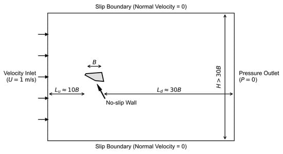
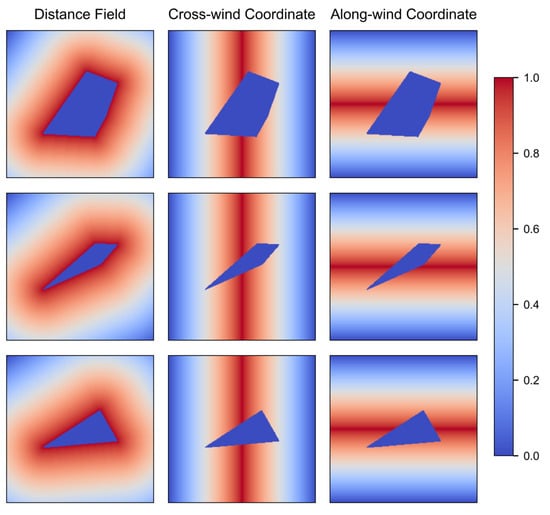
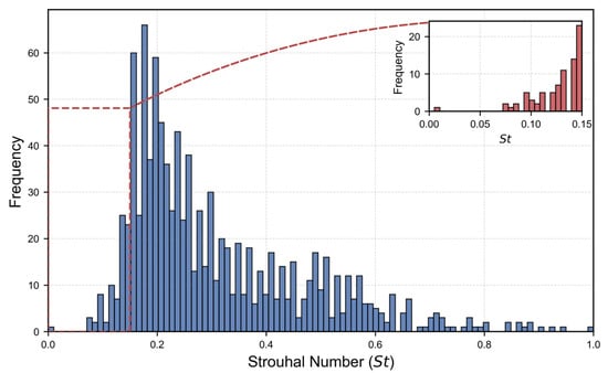
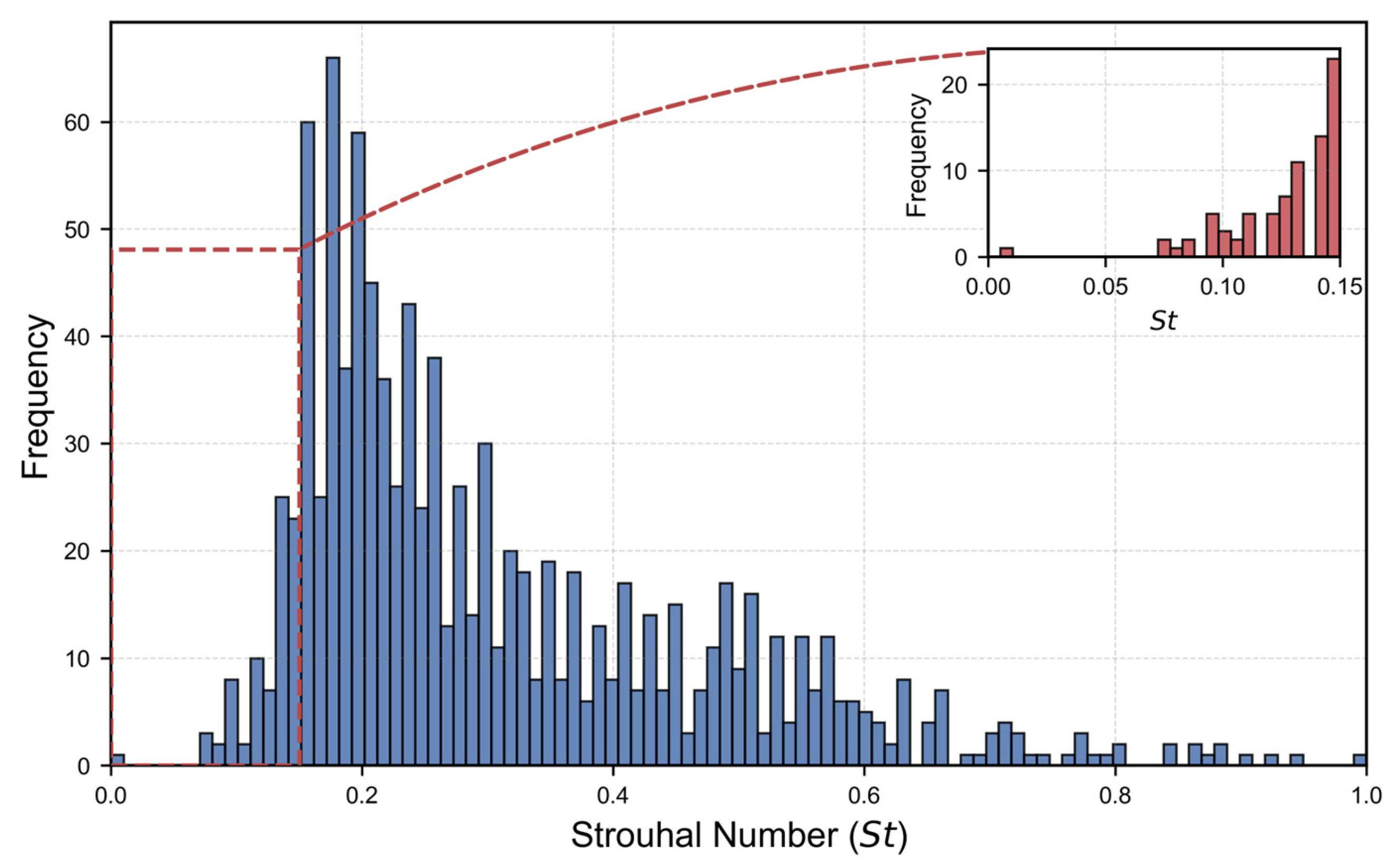
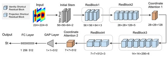
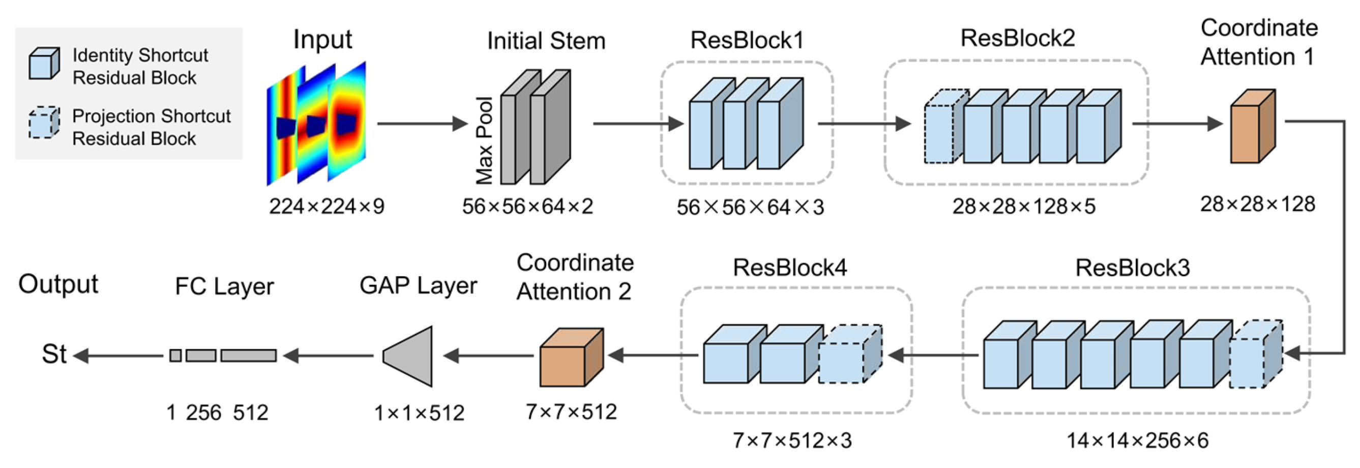
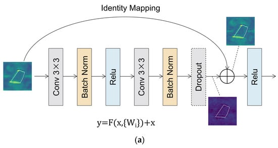
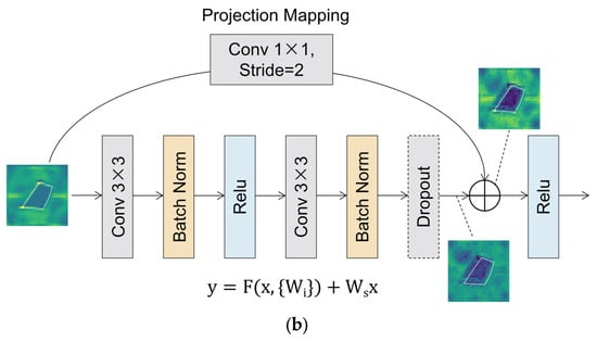
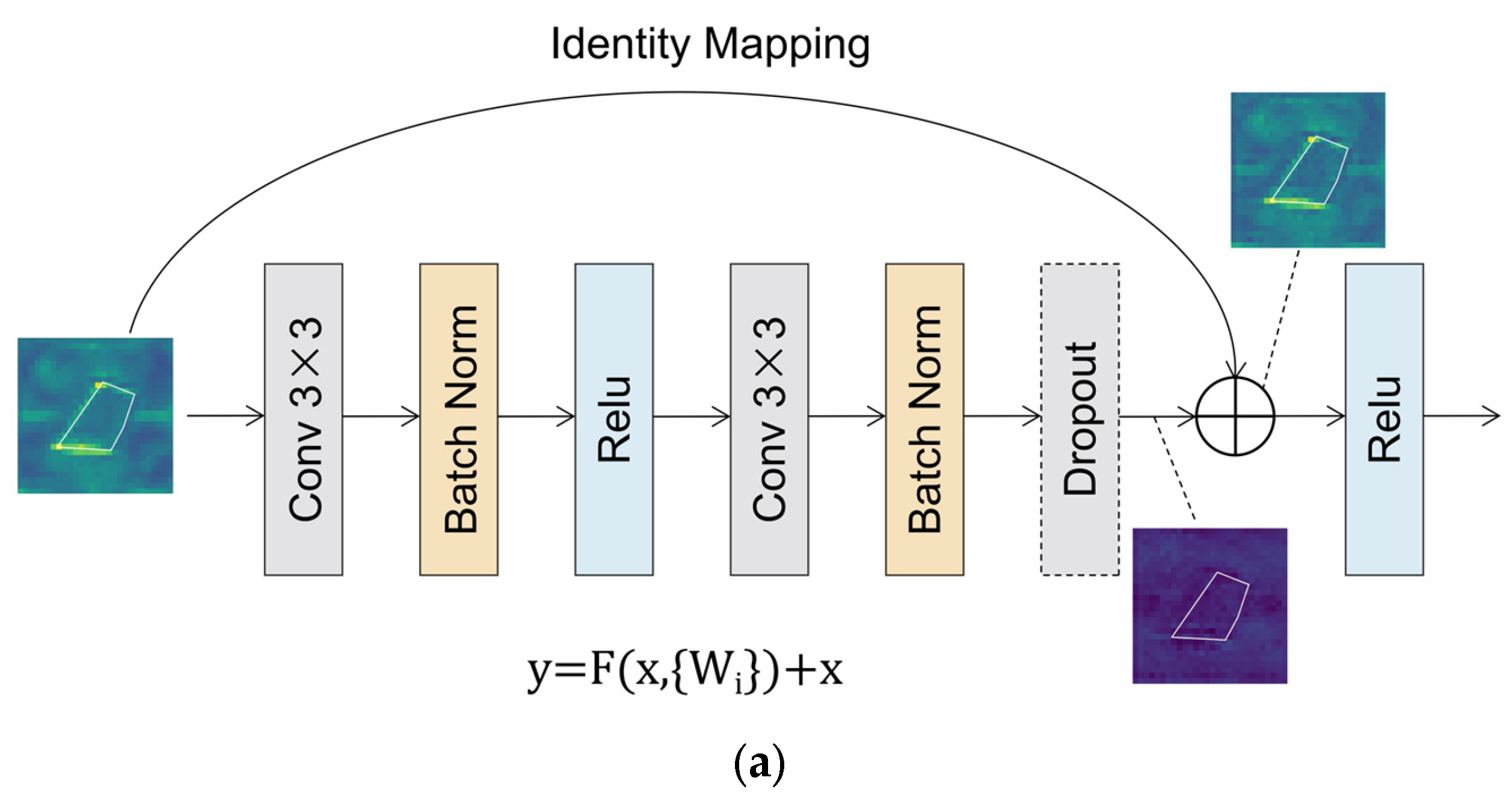
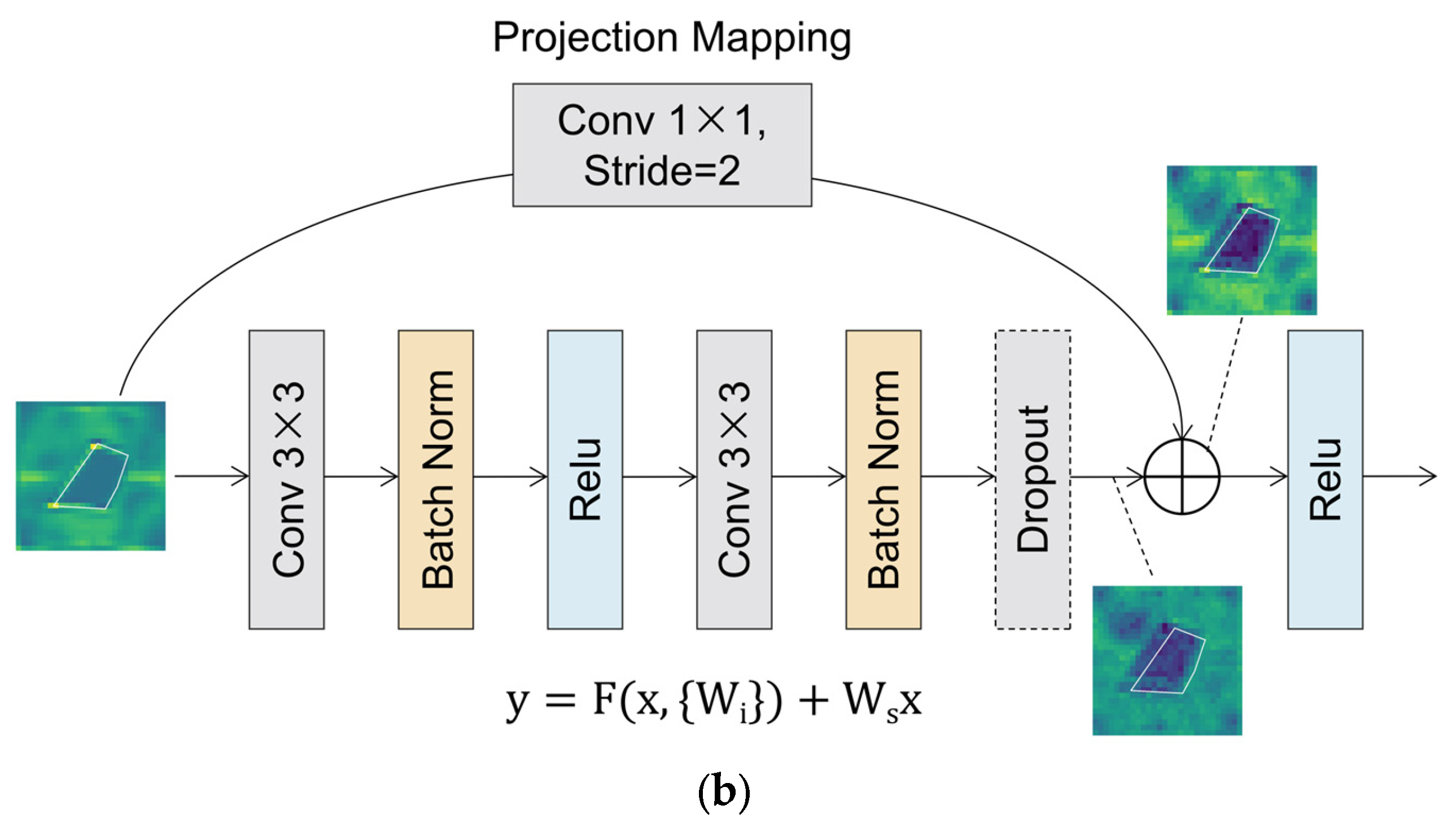
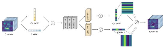
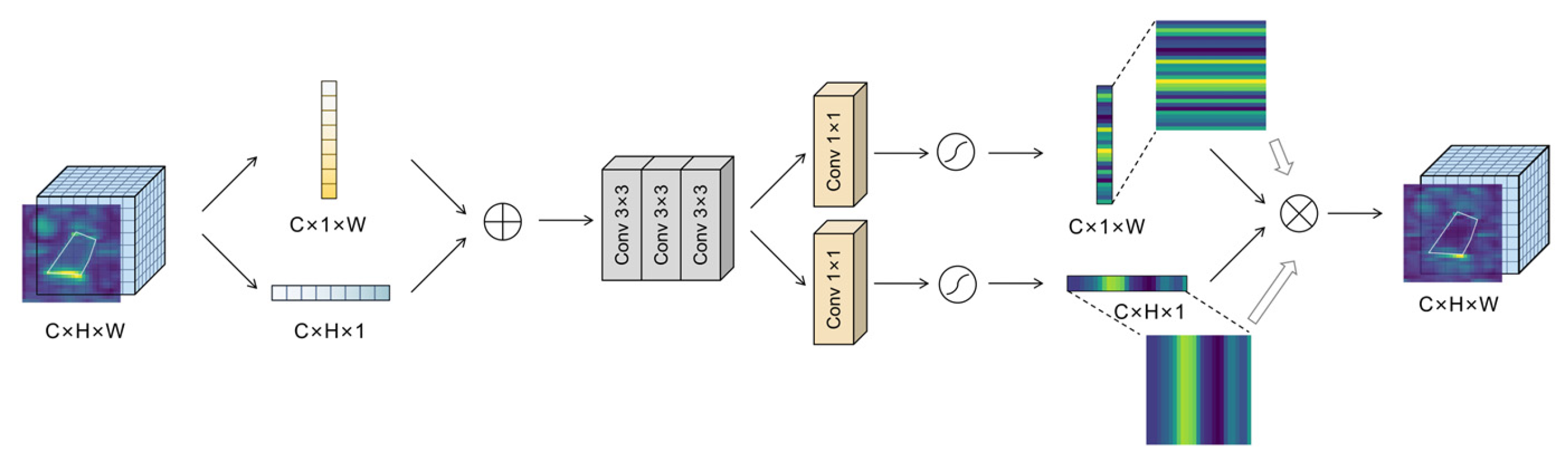
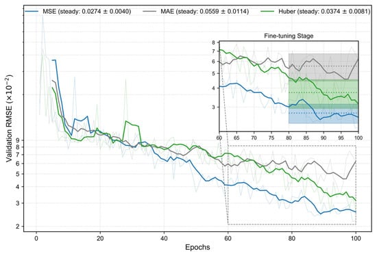
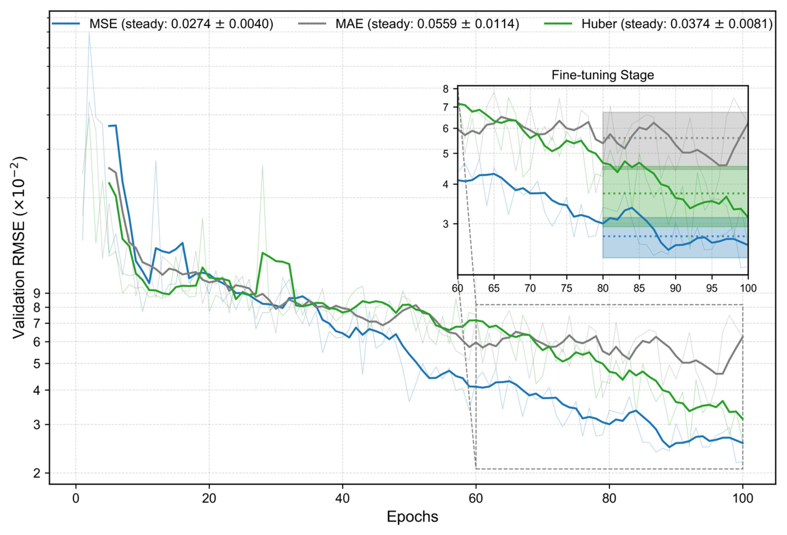
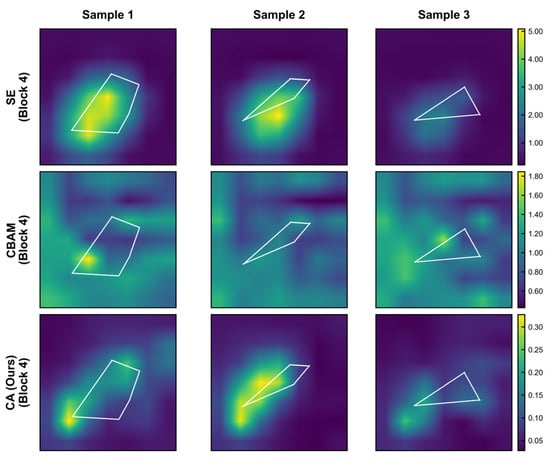
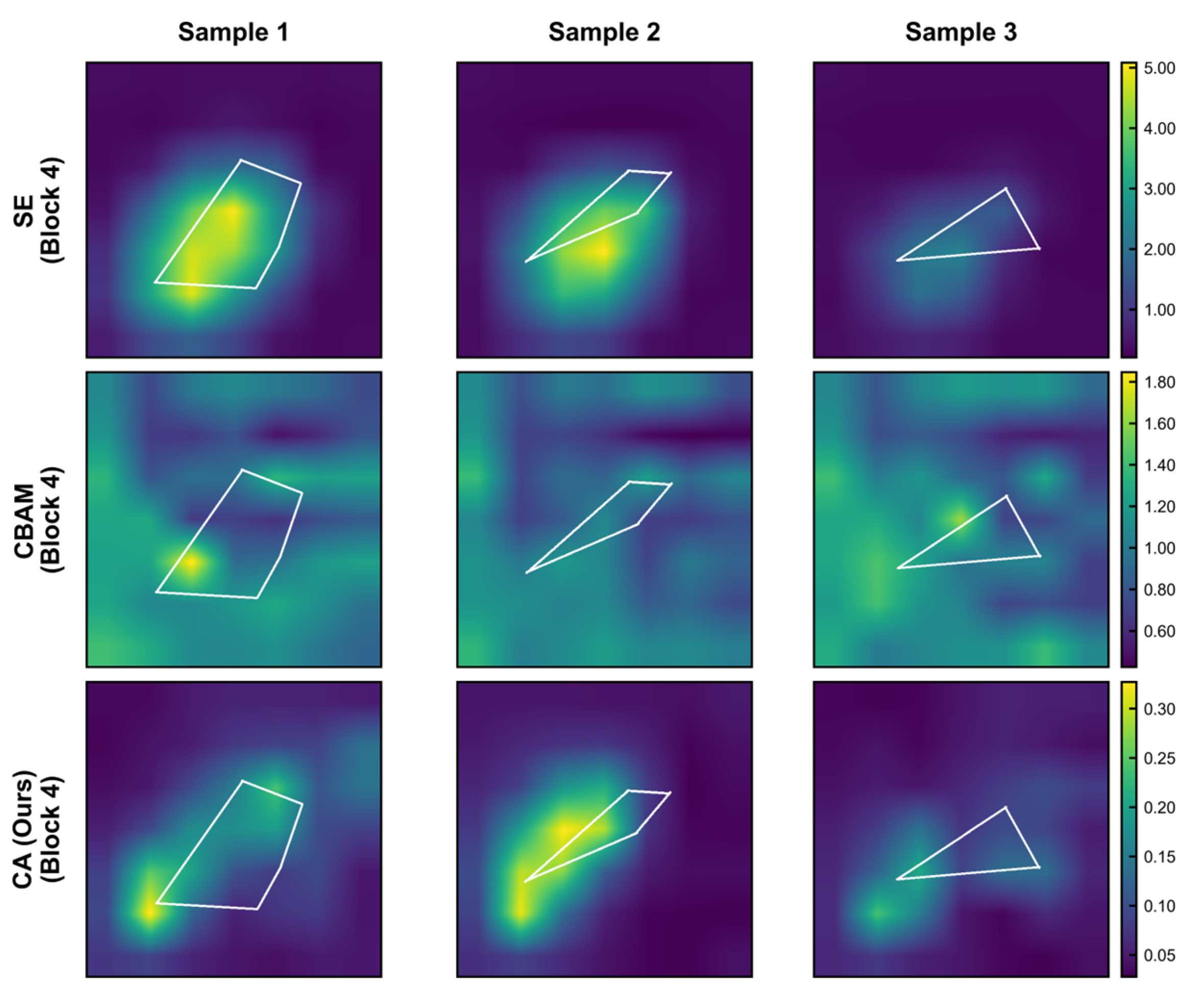
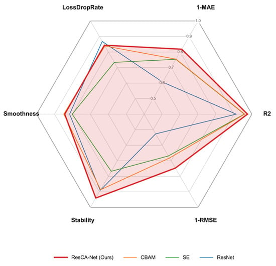
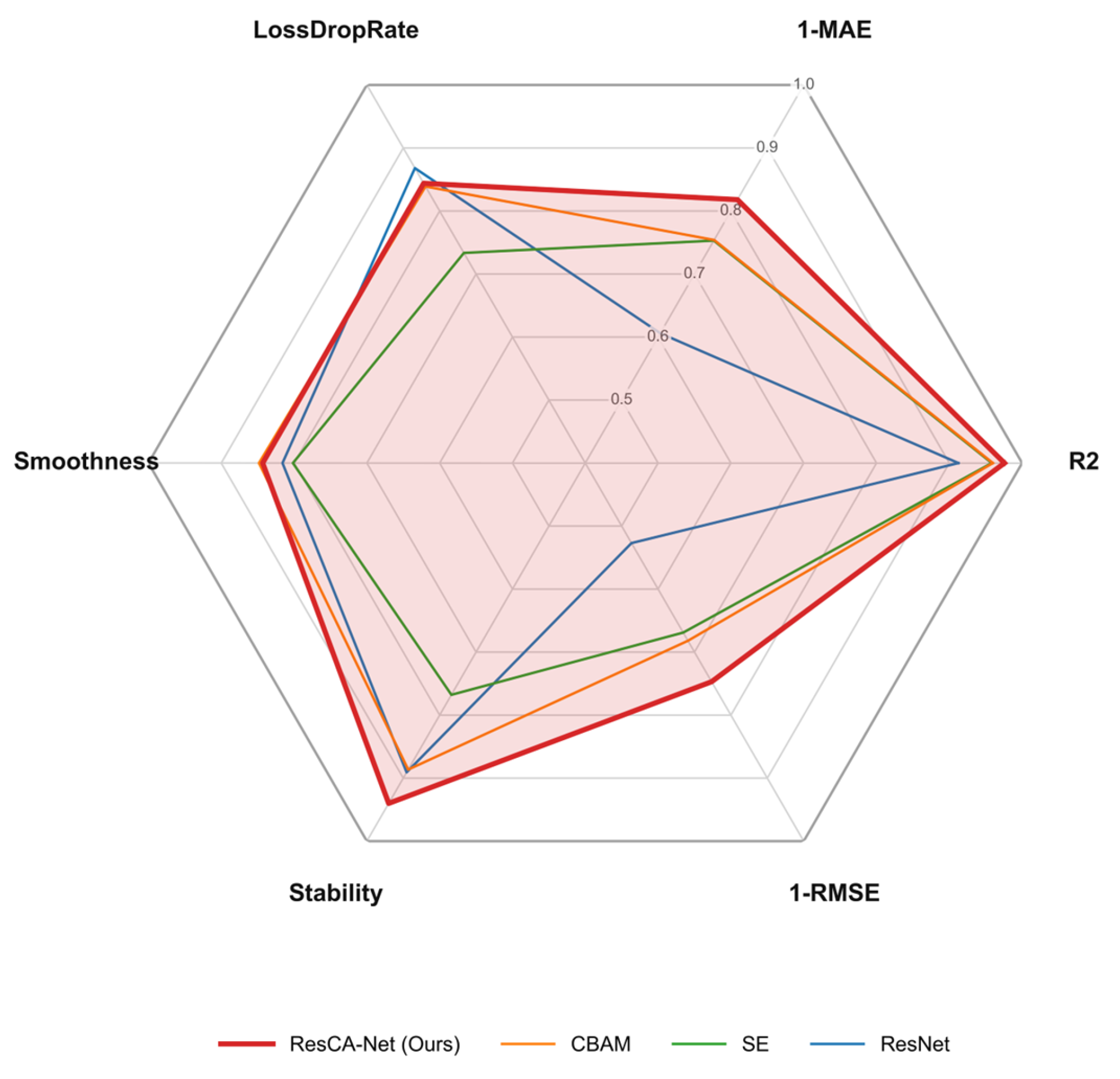
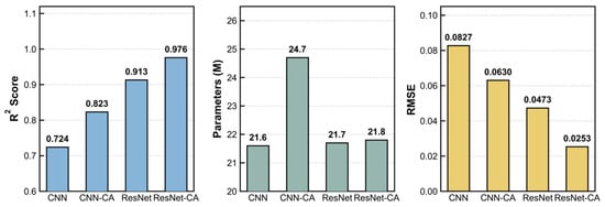
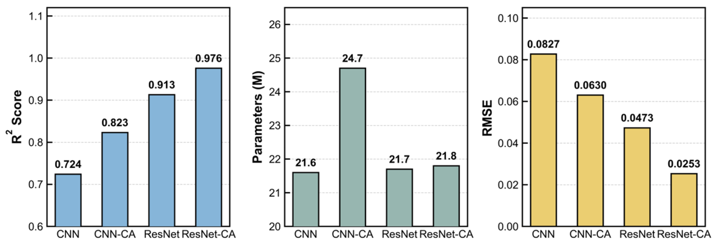
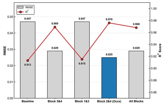
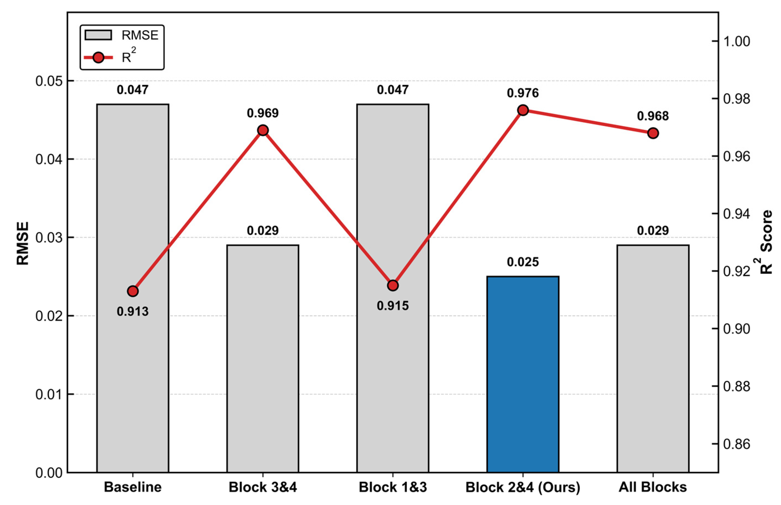
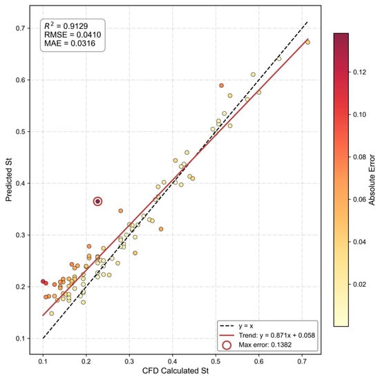
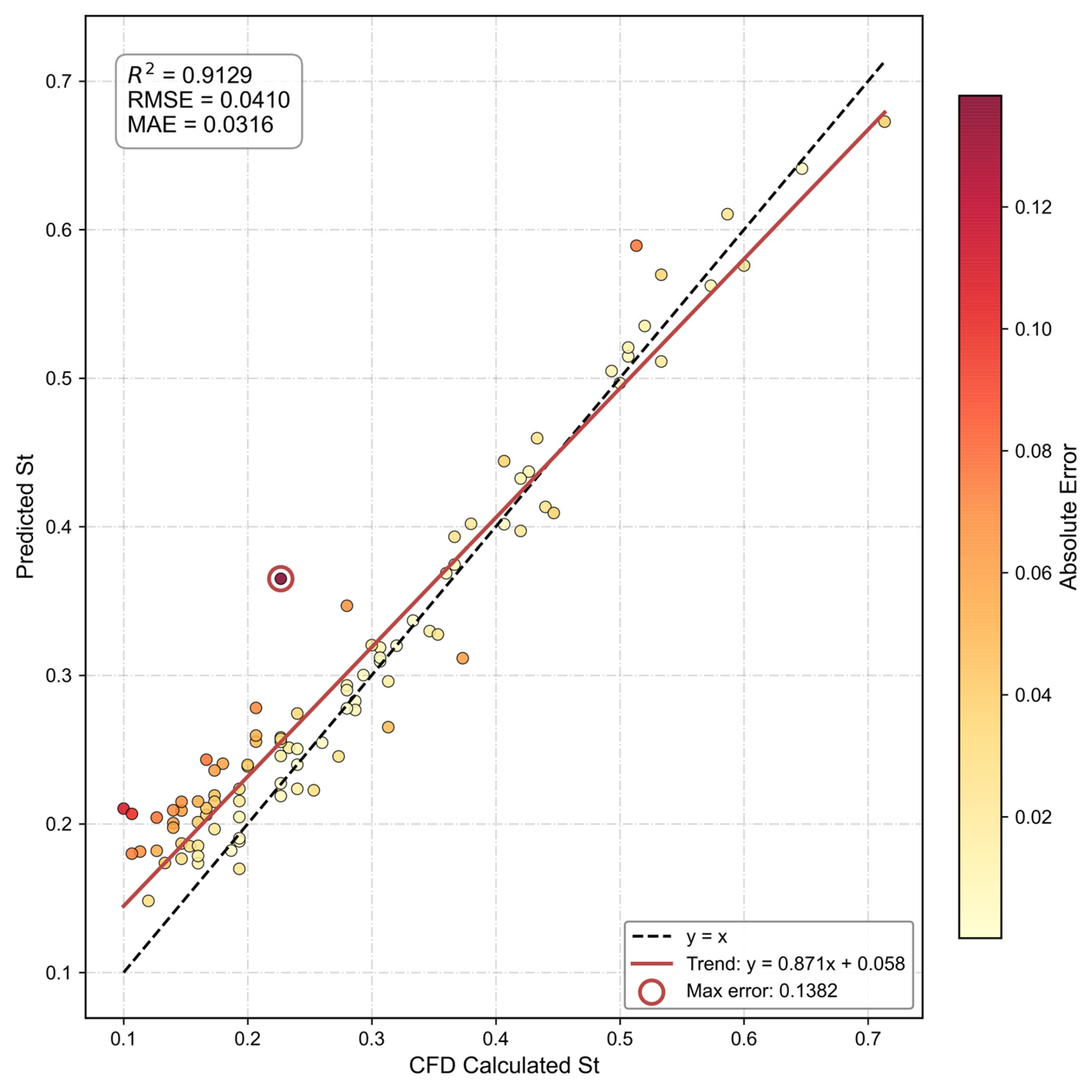
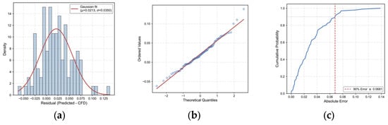
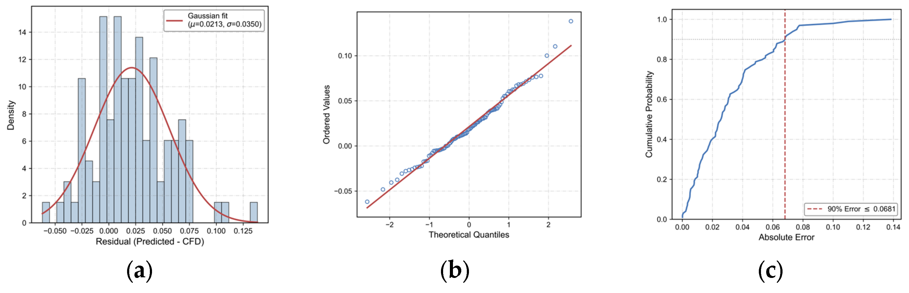
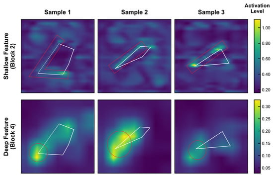
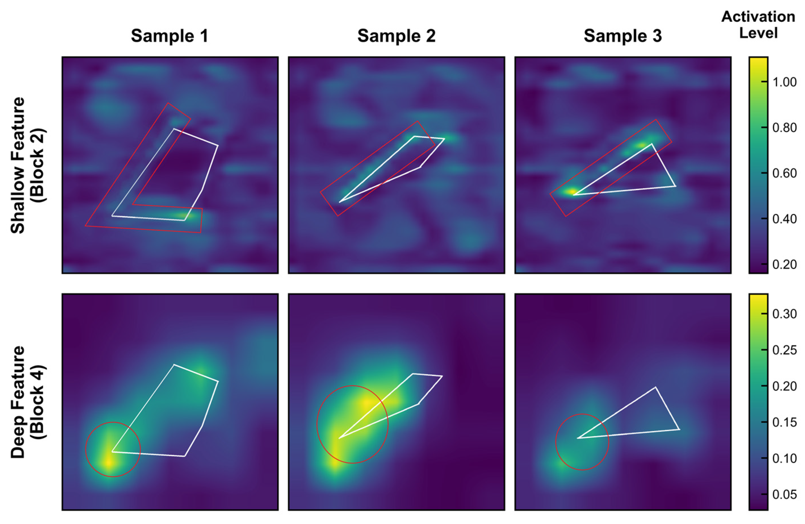
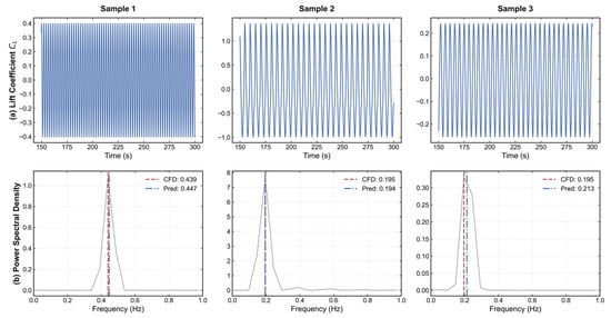
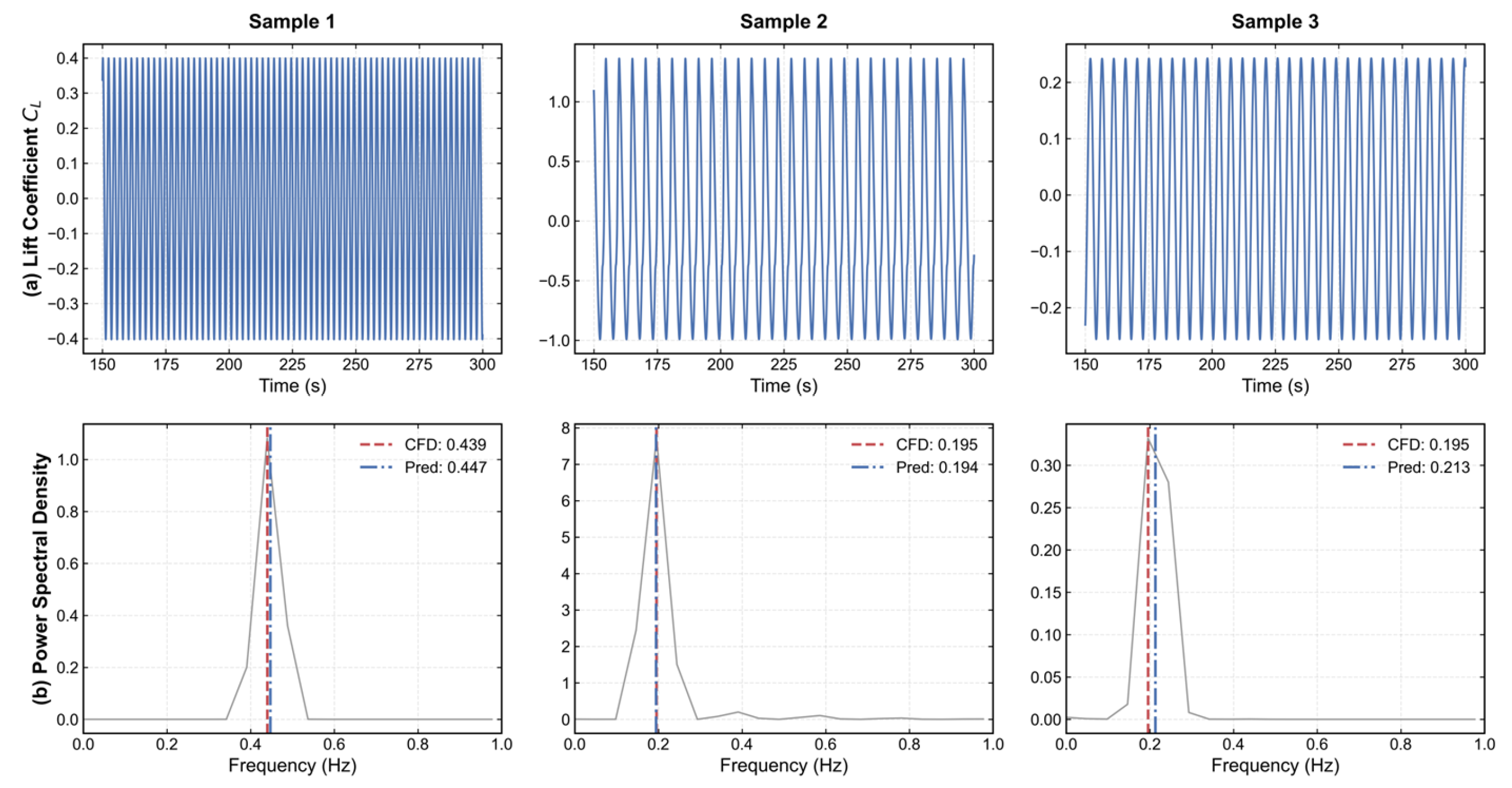

Disclaimer/Publisher’s Note: The statements, opinions and data contained in all publications are solely those of the individual author(s) and contributor(s) and not of MDPI and/or the editor(s). MDPI and/or the editor(s) disclaim responsibility for any injury to people or property resulting from any ideas, methods, instructions or products referred to in the content. |
© 2026 by the authors. Licensee MDPI, Basel, Switzerland. This article is an open access article distributed under the terms and conditions of the Creative Commons Attribution (CC BY) license.