


Abstract
Runway occupancy time (ROT) is a key indicator affecting runway capacity, arrival spacing control, and airport surface operational safety. ROT is jointly influenced by multi-source heterogeneous factors, including aircraft performance, speed profiles, taxi distance, runway exits, meteorological conditions, and airport operational states. However, existing methods still face challenges in simultaneously modeling feature–expert adaptation, sample-level expert reliability, and predictive uncertainty. To address these issues, this paper proposes an uncertainty-aware scenario-adaptive feature ensemble learning framework, termed U-SAFE. The framework achieves expert-specific adaptation of multi-source features through shared-specific feature assignment and adaptive feature gating, constructs four heterogeneous experts including CatBoost, TabNet, TCN, and NGBoost, and designs a dynamic Softmax fusion mechanism based on predictive uncertainty, historical reliability, and scenario matching degree. A residual calibration module is further introduced to correct fusion bias and provide uncertainty estimates. Experiments were conducted on 15,030 landing samples collected from Xi’an Xianyang, Chengdu Tianfu, and Guangzhou Baiyun airports. The results show that U-SAFE achieves MAE, RMSE, and MAPE values of 2.97 s, 3.92 s, and 5.96%, respectively, on the overall test set, outperforming conventional models, including individual base learners and traditional stacking. Airport-specific testing, cross-airport generalization, scenario-based robustness analysis, and ablation studies further demonstrate stable predictive performance under the evaluated settings and verify the effectiveness of the key modules. Uncertainty analysis shows that U-SAFE obtains an NLL of 2.78, a PICP of 94.6%, and an MPIW of 15.6 s, indicating that it can provide reliable and compact prediction intervals while maintaining high predictive accuracy. These results demonstrate that U-SAFE can effectively support accurate ROT prediction and uncertainty-aware decision-making in complex airport operating environments. Nevertheless, the present findings should be interpreted within the scope of the three-airport dataset and the February 2025–May 2026 observation window. Complete airport topology and human-related operational factors are not explicitly represented, while prospective temporal validation and deployment-level inference latency remain to be further evaluated.
1. Introduction
Runway occupancy time (ROT) generally refers to the time interval from the moment an aircraft crosses the runway threshold during landing to the moment it completely vacates the runway [1]. As a key temporal parameter in airport surface operations, ROT directly affects arrival separation, runway capacity, runway-exit utilization, arrival sequencing, and tower–approach coordination. Under safety constraints, runway throughput is jointly determined by aircraft separation requirements and runway occupancy characteristics, making ROT prediction an important component of runway capacity enhancement and operational decision support [2,3,4,5]. In particular, as reduced arrival-separation procedures are increasingly introduced, prolonged or highly variable ROT may become a binding constraint that prevents the theoretical capacity benefits of smaller approach spacing from being fully realized [6,7]. In high-density airport operations, even small variations in ROT may therefore lead to arrival-spacing adjustments, reduced runway throughput, or potential operational conflicts. Accurate ROT prediction is thus essential for improving runway utilization, reducing operational risks, and supporting intelligent air traffic management decision-making.
Previous studies have investigated ROT from different perspectives, including influencing-factor analysis, runway throughput assessment, runway-exit selection, abnormal occupancy detection, and data-driven prediction. Early airside simulation and operational studies established runway occupancy as an important determinant of runway performance and showed that occupancy characteristics vary with aircraft and operational conditions [8,9]. Analyses based on airport surface surveillance data subsequently enabled flight-level ROT extraction and revealed systematic relationships between occupancy behavior and aircraft/runway characteristics [10,11], while abnormal ROT and its operational precursors were explicitly investigated using data-driven methods [12]. The stochastic nature of ROT has also been linked to arrival delay and sequencing performance [13,14]. In addition to these operational effects, landing-roll dynamics and runway infrastructure play important roles in determining runway-vacation behavior. Braking profiles can directly affect landing-roll distance and ROT [15], while the geometry and longitudinal location of high-speed or rapid exit taxiways influence the opportunity for aircraft to vacate the runway efficiently [16,17]. Recent empirical analysis has confirmed that favorable rapid-exit-taxiway placement can substantially reduce runway occupancy time, with effects that differ across aircraft categories [18]. These findings show that ROT is jointly shaped by aircraft dynamics, runway-exit infrastructure, and operational conditions, and that its variability has direct implications for runway utilization and arrival-flow efficiency.
With the increasing availability of airport surveillance and flight-operation data, ROT research has gradually evolved from statistical characterization toward flight-level predictive modeling [19,20]. Simulation-based and predictive models have been developed for runway-exit design, arrival/departure occupancy time, and related runway-performance estimation [21,22]. Runway-exit choice and related airport-surface operational variables have also been addressed using machine-learning, support-vector, and causal-learning approaches [23,24,25]. For arrival ROT itself, neural-network and CNN-based models have been developed to capture nonlinear relationships among landing and operational variables [26,27,28], while tree-based feature-equivalence strategies have been investigated to improve cross-airport model generalization [29]. Other studies have considered real-time prediction of runway occupancy buffers [30], joint prediction of arrival ROT and exit taxiway using ADS-B trajectories [31], and QAR-based machine-learning prediction with hybrid optimization and interpretability analysis [32]. Boosted-tree and feedforward-neural-network frameworks have further linked runway occupancy prediction with runway-exit or exit-distance estimation [33,34]. More recently, runway-exit prediction has incorporated heterogeneous information including ASDE-X trajectories, aircraft characteristics, traffic-flow indicators, ramp information, and meteorological variables, together with probabilistic calibration metrics [35]. Deep learning-based studies of related runway-occupation prediction have also introduced multi-scale temporal convolution and xLSTM–Transformer architectures to capture complex temporal dependencies and high-dimensional feature interactions [36,37].
These studies demonstrate that ROT prediction is a multi-source heterogeneous and scenario-dependent problem, jointly influenced by aircraft performance, speed profiles, runway exits, flight trajectories, meteorological conditions, and operational states. Despite these advances, several limitations remain. First, ROT is affected by heterogeneous factors with different data structures, including categorical operational attributes, continuous speed and trajectory variables, temporal traffic-flow dependencies, and environmental conditions. A single model type is often insufficient to capture these diverse relationships simultaneously. Second, many existing ROT predictors rely on a single learning paradigm, while ensemble-oriented or multi-model studies generally emphasize prediction performance rather than explicit adaptation between heterogeneous feature structures and complementary base learners. This may limit expert diversity and complementary learning. Third, airport operations are highly scenario-dependent; adverse conditions such as thunderstorms, low visibility, and strong winds can alter both feature importance and model reliability. Although recent research has incorporated increasingly rich trajectory, traffic, aircraft, and weather contexts, sample-level adaptation of expert reliability under changing operational scenarios remains insufficiently explored. Fourth, uncertainty is an inherent property of ROT. Existing work has considered stochastic occupancy effects, sequencing uncertainty, and real-time occupancy buffers; however, most learning-based ROT predictors still emphasize deterministic point-estimation accuracy, with comparatively limited attention to calibrated predictive uncertainty and residual calibration. This restricts their applicability to trustworthy and risk-aware decision-making in safety-critical airport operations.
To address these limitations, this paper proposes an uncertainty-aware scenario-adaptive feature ensemble learning framework, termed U-SAFE, for aircraft landing ROT prediction. The framework first performs aviation context-aware feature processing through shared-specific feature assignment and adaptive feature gating, enabling expert-specific utilization of multi-source features. It then constructs four heterogeneous experts, namely CatBoost, TabNet, TCN, and NGBoost, to capture categorical structural rules, nonlinear feature interactions, temporal operational dependencies, and probabilistic uncertainty, respectively. A reliability-aware dynamic fusion layer further computes sample-specific expert weights based on predictive uncertainty, historical reliability, and scenario matching degree. Finally, a residual calibration layer corrects systematic fusion bias and generates calibrated ROT predictions with uncertainty representation. Through this design, U-SAFE provides a complete prediction pipeline from feature-aware expert adaptation to uncertainty-aware dynamic fusion and residual-calibrated output.
2. ROT Formation Mechanism and Multi-Source Feature Analysis
2.1. Definition and Predictive Significance of ROT
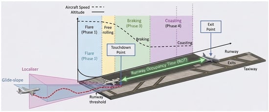
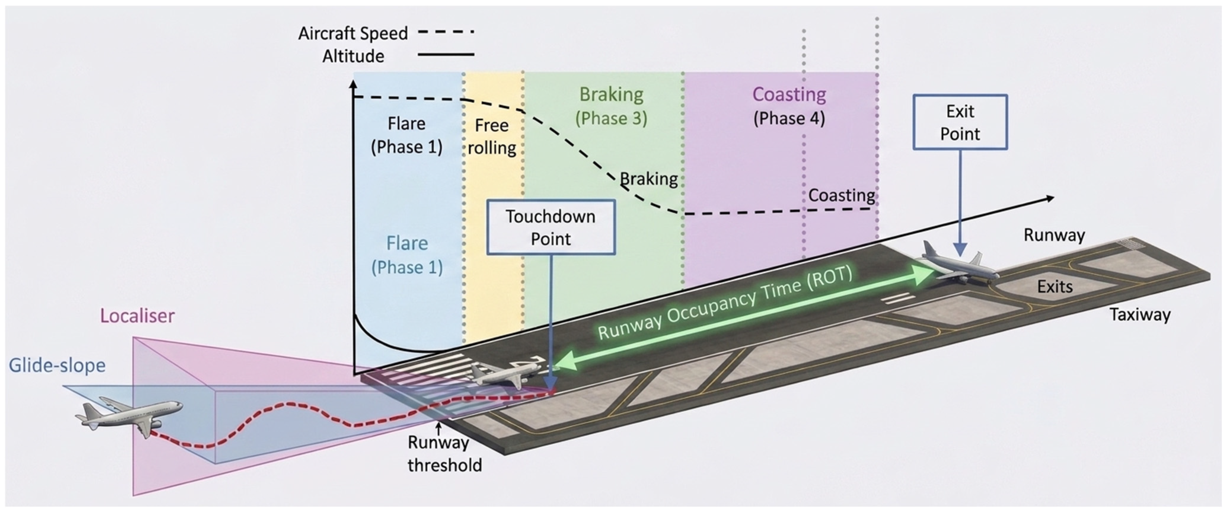
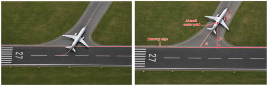
Aircraft landing is a continuous dynamic process in which an aircraft transitions from the airborne approach phase to the ground roll phase. During landing, the aircraft typically follows a predefined glide path into the final approach, maintains a relatively stable attitude and speed near the runway threshold, and then crosses the threshold, flares, touches down, decelerates, rolls out, and finally exits the runway via an appropriate exit taxiway. For landing aircraft, runway occupancy time is generally defined as the time interval from the moment the aircraft crosses the runway threshold to the moment its tail completely vacates the runway, as illustrated in Figure 1. The landing process can be divided into several sequential phases from final approach to runway vacation. Before reaching the runway threshold, the aircraft follows the glide path and enters the flare phase, during which its altitude decreases, and the touchdown state is prepared. The ROT measurement starts when the aircraft crosses the runway threshold. From an aerospace-engineering perspective, the touchdown point and the subsequent runway-occupancy process are closely related to the aircraft energy state and longitudinal dynamics during approach and landing. Approach speed, glide-path characteristics, and flare behavior affect the touchdown position and touchdown speed, which in turn determine the remaining ground-roll distance and the kinetic energy that must be dissipated before runway vacation. After touchdown, aerodynamic drag, wheel braking, reverse thrust, rolling resistance, and runway-surface friction jointly govern the deceleration process, while the geometry and location of the selected runway exit constrain the feasible exit speed and turning maneuver. Consequently, variations in touchdown state, deceleration capability, and runway-exit conditions can directly lead to differences in ROT. When the aircraft approaches the assigned exit taxiway, it enters a coasting and turning phase until the aircraft tail completely clears the runway boundary. Therefore, ROT is not determined only by the touchdown point or exit location, but is jointly affected by approach speed, touchdown state, deceleration performance, runway-exit geometry, surface condition, and exit maneuver. This process-level interpretation also explains why ROT prediction requires multi-source operational, trajectory, environmental, and runway-configuration features.
Figure 1.
A schematic diagram of runway occupancy time.
ROT is an important parameter affecting runway operational efficiency and safety margins. Accurate ROT prediction can provide refined inputs for runway capacity assessment, support arrival sequencing and spacing optimization, assist in identifying long-occupancy risks, and contribute to runway-exit planning, surface taxi coordination, and intelligent airport operation decision-making. One potential operational environment in which such predictive information may be utilized is the Advanced Surface Movement Guidance and Control System (A-SMGCS), which supports the surveillance, routing, guidance, and control of aircraft and vehicles on the airport surface. Although ROT prediction is not a primary function of A-SMGCS, reliable ROT estimates could complement surface-management activities by providing additional predictive information for runway-occupancy monitoring and runway-exit coordination.
ROT variability is also influenced by meteorological and human-related operational factors. Adverse conditions such as strong winds, low visibility, precipitation, and degraded runway-surface conditions may affect approach stability, touchdown state, braking effectiveness, and runway-exit behavior. In addition, flight-crew operating behavior and air traffic control instructions may further contribute to variations in runway-vacation time. Importantly, ROT prediction is intended to support safety-aware operational decision-making rather than to encourage unnecessarily rapid runway vacation; established flight-safety requirements and standard operating procedures remain the primary constraints of runway operations. It should be noted that the present study focuses exclusively on arrival ROT. Departure runway occupancy involves a distinct operational and dynamic sequence, including runway entry, line-up, takeoff roll, rotation, and liftoff, and is therefore outside the scope of the current study.
2.2. Airport Infrastructure Factors Related to ROT
Airport infrastructure provides the physical and operational environment within which arrival runway occupancy time is generated. From an airport-system perspective, ROT is not determined solely by aircraft performance and landing dynamics; it is also constrained by the spatial organization and functional characteristics of the airside infrastructure. Among these elements, the runway system and the runway–taxiway interface are most directly related to the runway-occupancy process. The number and configuration of runways influence runway allocation, arrival–departure operating modes, and the potential interactions among simultaneous runway operations. Although runway count itself does not directly determine the ROT of an individual aircraft, different runway configurations may create different operational conditions, traffic patterns, and runway-use strategies, thereby affecting the context in which ROT is observed.
The layout of runway exits and connecting taxiways has a more direct physical relationship with ROT. The longitudinal position of an exit relative to the touchdown point determines the available ground-roll distance before runway vacation, while exit geometry and turning angle constrain the speed at which an aircraft can safely leave the runway. Consequently, different combinations of touchdown position, runway-exit location, exit angle, and taxiway connectivity may result in different deceleration requirements and runway-vacation times. Other airport infrastructure elements, including aprons, aircraft parking stands, and terminal layouts, are primarily associated with aircraft movements after runway vacation and therefore have a less direct relationship with the ROT interval itself. Nevertheless, their influence may propagate upstream through surface-traffic interactions. Therefore, airport infrastructure should be viewed as a hierarchical set of factors affecting ROT: runway geometry, runway-exit configuration, and connecting taxiways exert relatively direct effects on the runway-vacation process, whereas apron, stand, and terminal configurations mainly contribute through indirect surface-traffic and operational interactions.
2.3. Extraction and Analysis of Multi-Source Features
ROT is jointly influenced by multiple factors, including aircraft type, speed state, runway exit, meteorological conditions, and flight trajectory. To comprehensively characterize the runway occupancy process of landing aircraft, this study constructs multi-source features from six perspectives for ROT prediction: aircraft and operations, speed profile, environmental conditions, runway exit, flight trajectory, and operational mode and separation, as shown in Table 1.
Table 1.
Multi-source features and mechanisms affecting ROT prediction.
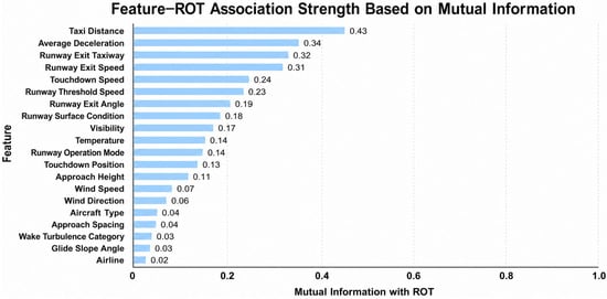
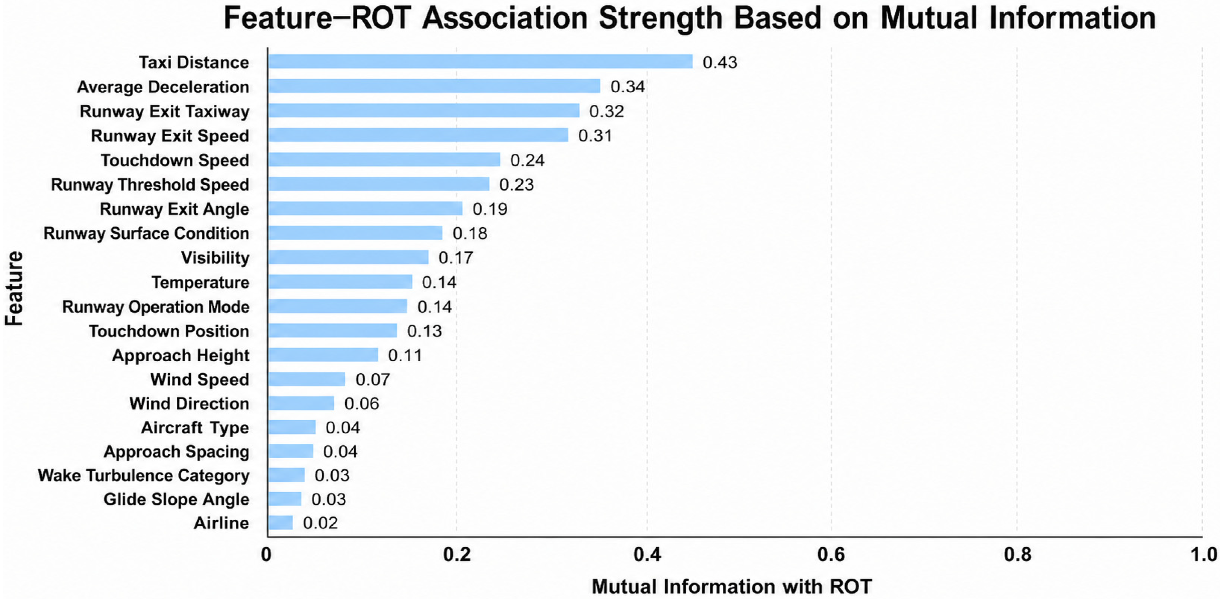
The 20 input features were constructed based on the physical formation mechanism of ROT, aviation operational knowledge, existing ROT-related studies, and the availability of reliable multi-source operational data. Specifically, landing ROT is determined by the continuous process from runway-threshold crossing to runway vacation, which involves aircraft performance, speed state, touchdown behavior, deceleration capability, runway-exit configuration, meteorological environment, and operational constraints. Because the input variables contain different feature types, targeted preprocessing strategies were adopted. After abnormal samples were removed and missing values were handled, categorical features were encoded using embedding representations, continuous features were standardized and robustly normalized to reduce the influence of scale differences, and cyclic variables were transformed using sine–cosine encoding. A total of 15,030 valid landing samples were collected from the corresponding runways of Xi’an Xianyang Airport, Chengdu Tianfu Airport, and Guangzhou Baiyun Airport, with each sample containing 20 features. After feature preprocessing, the mutual information (MI) between each feature and ROT was calculated, and the normalized MI results are shown in Figure 2. The results indicate that ROT is mainly affected by ground-roll distance after touchdown, deceleration capability, and runway-exit-related control factors. Environmental conditions, operational organization, and touchdown position also influence ROT, but their effects are usually coupled with speed, deceleration, and exit-related features. In contrast, the remaining features show relatively weaker individual statistical dependence on ROT.
Figure 2.
Mutual information-based feature relevance to ROT.
3. U-SAFE Framework for Runway Occupancy Time Prediction
3.1. U-SAFE Framework
Aircraft landing runway occupancy time is jointly determined by multi-source heterogeneous factors, including aircraft performance, speed states, runway exits, trajectory characteristics, meteorological conditions, and operational context. Therefore, an effective ROT prediction model should not only capture nonlinear relationships among heterogeneous features, but also adapt to changing operational scenarios and quantify predictive uncertainty. However, single models usually focus on limited information structures, while conventional stacking methods often use identical input features and static or implicitly learned fusion strategies. As a result, they may insufficiently model feature–expert adaptation, sample-level expert reliability, and uncertainty-aware decision-making. These limitations motivate the development of a feature-aware, dynamically weighted, and uncertainty-calibrated ensemble framework.
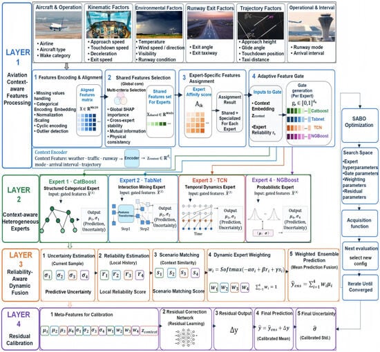
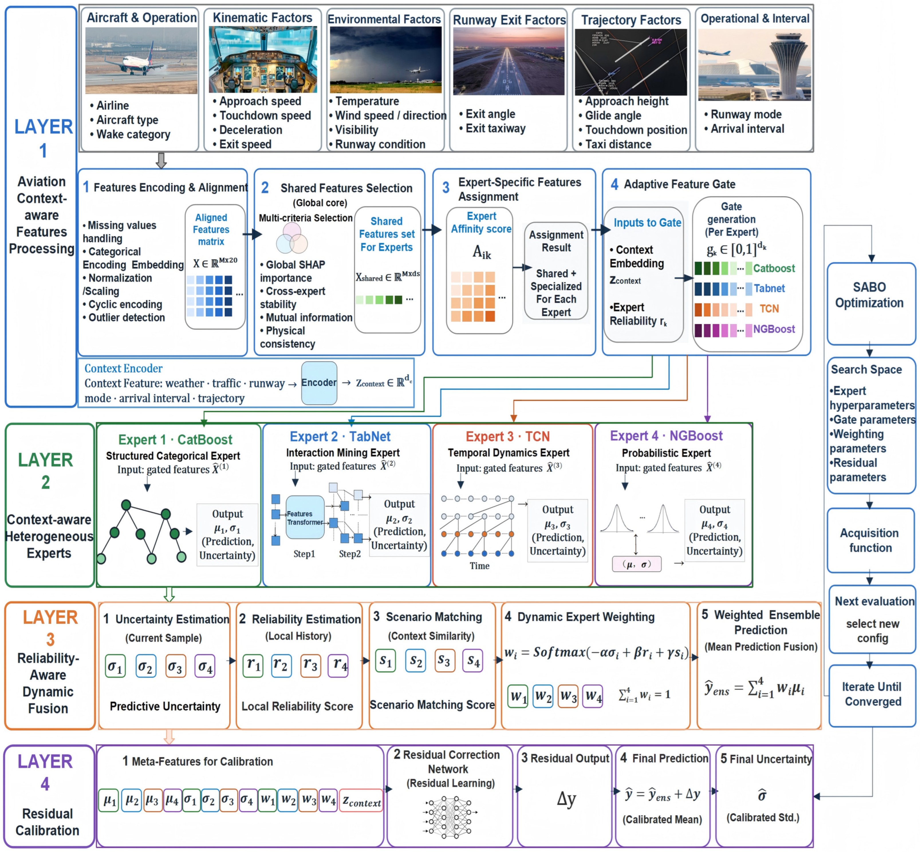
To address these issues, a four-layer U-SAFE framework is proposed for ROT prediction, as shown in Figure 3. The Aviation Context-aware Feature Processing Layer encodes multi-source features, selects shared features, assigns expert-specific features, and adaptively gates expert inputs according to the current operational context. The Context-aware Heterogeneous Expert Layer constructs CatBoost, TabNet, TCN, and NGBoost experts to capture categorical structural rules, nonlinear feature interactions, temporal operational dependencies, and probabilistic uncertainty, respectively. The Reliability-aware Dynamic Fusion Layer computes sample-specific expert weights based on predictive uncertainty, historical reliability, and scenario matching, enabling adaptive expert routing under different operating conditions. Finally, the Residual Calibration Layer corrects systematic fusion bias using the outputs of the four base learners, including their predicted values, predictive uncertainties, dynamic weights, and contextual embeddings, producing calibrated ROT predictions with uncertainty representation.
Figure 3.
Overview of the proposed framework for ROT prediction.
3.2. Aviation Context-Aware Feature Processing Layer
3.2.1. Feature Encoding and Alignment
The input variables include categorical, continuous, cyclical, and state-related features. To ensure the effective utilization of multi-source information, the raw features are first encoded and aligned before model training. Categorical features are encoded using an embedding mechanism, as shown in Equation (1):
Continuous features are standardized, as shown in Equation (2):
Cyclical features (wind direction) are transformed using sine–cosine encoding in Equation (3):
After preprocessing, a unified feature matrix is obtained in Equation (4):
3.2.2. Shared Feature Selection
After feature encoding and alignment, shared features need to be selected from the 20 input variables for the four base learners. These shared features are not simply the most correlated variables, but core variables that provide stable and consistent information for all experts. Therefore, a multi-criteria scoring strategy is adopted to select shared features, as defined in Equation (5):
where denotes the global SHAP importance of the -th feature, represents its cross-expert stability, and denotes the mutual information-based relevance between the feature and ROT.
These terms are calculated according to Equations (6)–(8), respectively. In Equation (5), , and denote the normalized values, respectively. In Equation (6), denotes the number of base learners, is the number of training samples, denotes the -th training sample, and denotes the SHAP contribution of the -th feature in the -th base learner to the prediction for sample . In Equation (7), denotes the normalized importance score of the -th feature estimated by the -th expert model using permutation importance. After multi-criteria aggregation, the features with higher scores and consistency with aviation operational mechanisms are selected as the shared feature set .
3.2.3. Expert-Specific Feature Assignment
In addition to shared features, each base learner is better suited to specific feature types. Therefore, feature–expert affinity is calculated to assign each feature to the expert with the highest suitability. The feature–expert affinity is defined in Equation (9):
where denotes the capability matching score, which measures the compatibility between the feature type and the inductive bias of the expert model; represents the performance gain, defined as the reduction in prediction error after incorporating the feature into the expert model; and denotes the expert diversity score, indicating whether the feature can enhance complementarity among experts. These three terms are calculated according to Equations (10)–(12), respectively.
where is the feature meta-description vector, including categorical, continuous, temporal, nonlinear, and uncertainty-related attribute scores, and denotes the bias vector of the expert model.
where denotes the baseline input feature set of the -th base learner, and represents the -th candidate feature. denotes the validation RMSE of the -th base learner before adding , whereas denotes the validation RMSE after incorporating . The term retains only the positive performance gain; if adding the candidate feature does not reduce the validation RMSE, its performance gain is set to zero.
where denotes the contribution vector of the j-th feature in the -th expert, is the number of expert models, indexes the other experts except the i-th expert, and is a small constant used to avoid division by zero. Equation (12) is used to compute the complementarity score of the -th feature for the -th base learner. Specifically, the absolute cosine similarity is first calculated between the sample-level contribution vector of this feature in the -th base learner and its contribution vectors in the other base learners. The similarities are then averaged over the remaining M − 1 base learners to obtain the average contribution-pattern similarity. Finally, is obtained by subtracting this average similarity from one. A lower average similarity indicates that the feature provides more distinctive and complementary information for the -th base learner, resulting in a larger . Finally, each feature is assigned to the expert with the highest affinity score according to Equation (13), meaning that the -th feature is allocated to the most suitable -th expert model.
It should be noted that the SHAP-, permutation-, and contribution-based quantities used in the shared and expert-specific feature assignment procedures are computed during offline model construction. Once the feature sets are determined, these quantities are not recalculated for each incoming sample during online inference.
3.2.4. Context Encoder
The context encoder is used to characterize the current aviation operational state, including weather conditions, runway status, approach spacing, operation mode, and trajectory state. denotes the context feature vector. The context embedding is obtained using a lightweight MLP, as defined in Equations (14) and (15).
3.2.5. Adaptive Feature Gate
After shared feature selection and expert-specific feature assignment, the importance of the same input features may still vary across different operational scenarios. Therefore, this study introduces an adaptive feature gate (AFG) to address the dynamic scenario-adaptation problem of how strongly each feature should be activated for the current sample. Let denote the gate vector of the -th expert, as defined in Equation (16). represents the combination of shared and expert-specific features for expert , and denotes the final gated input, which is obtained through the Hadamard product with the corresponding expert model in Equation (17).
3.3. Context-Aware Heterogeneous Expert Layer
The heterogeneous expert layer consists of four complementary base learners: CatBoost, TabNet, TCN, and NGBoost. CatBoost is used to capture categorical and structured rule-based features, such as airline, aircraft type, wake turbulence category, runway exit, and operation mode. TabNet focuses on deep nonlinear interactions among speed, environmental, and trajectory-related features. TCN models temporal dependencies associated with historical operating patterns, historical ROT, approach-spacing variations, and weather evolution. NGBoost serves as the probabilistic expert and directly outputs the predictive distribution. Each expert produces a predictive mean and an uncertainty estimate, denoted as . Specifically, CatBoost uses quantile-based uncertainty estimation, TabNet and TCN adopt MC Dropout, and NGBoost provides distributional uncertainty directly. These heterogeneous outputs provide complementary information for the subsequent reliability-aware dynamic fusion layer. To further assess whether the additional representational diversity of the four-expert architecture justifies its increased complexity, a reduced configuration retaining only CatBoost and TCN is additionally evaluated in Section 4.9 using the same dynamic weighting principle.
3.4. Reliability-Aware Dynamic Fusion Layer
3.4.1. Uncertainty Estimation
Each expert model outputs a predictive uncertainty . To ensure a consistent scale, the uncertainty values are normalized according to Equation (18). A larger uncertainty indicates that the corresponding expert is less stable for the current sample, and therefore its fusion weight should be reduced.
3.4.2. Reliability Estimation
Local reliability measures the performance of each expert in historical operational scenarios similar to the current sample. Based on the context embedding , similar historical samples are retrieved, as defined in Equation (19). The local error of the -th expert on these samples is then calculated according to Equation (20). This error is further converted into the reliability score . Unlike the offline feature-assignment calculations, historical-neighbor retrieval is performed during inference and therefore introduces additional online computational overhead. The present study focuses on evaluating predictive effectiveness, and end-to-end inference latency under operational deployment conditions has not yet been systematically benchmarked.
3.4.3. Scenario Matching
Scenario matching measures the similarity between the current operational state and the advantageous scenario of each expert model, as defined in Equation (22). denotes the scenario prototype vector in which the -th expert performs well, and denotes the scenario-matching score of the -th base learner, which quantifies how well the current operational context matches the scenario prototype where this learner is expected to perform reliably.
3.4.4. Dynamic Expert Weighting
The dynamic fusion weights of the expert models are calculated according to Equation (23). This mechanism adaptively adjusts the contribution of each expert based on the predictive uncertainty, historical reliability, and operational scenario of the current sample. , , and denote the normalized values of , , and , respectively. , , and are weighting coefficients controlling the contributions of uncertainty, reliability, and scenario matching, respectively. denotes the mean prediction of the -th expert model. The final weighted ensemble prediction is then obtained using Equation (24). Accordingly, the resulting fusion weights should be interpreted as conditional predictive allocations reflecting the joint effects of contextual similarity, predictive uncertainty, and historical reliability, rather than as causal effects of individual physical scenario factors.
3.5. Residual Calibration Layer
3.5.1. Residual Correction Network
The meta-learner is implemented as a residual correction module. The residual calibration network learns the residual between the dynamically fused prediction and the observed value, as defined in Equation (25). The meta-feature vector is constructed from the predicted mean, standard deviation, and dynamic weight of each expert model. Here, denotes a lightweight MLP, and the final prediction is obtained according to Equation (26).
3.5.2. Final Uncertainty Calibration
The final predictive uncertainty is jointly determined by the ensemble uncertainty of the experts and the magnitude of residual correction. The ensemble uncertainty is defined in Equation (27), and the final calibrated uncertainty is given in Equation (28). A larger residual correction indicates a greater deviation in the original fused prediction; therefore, the final uncertainty should be increased accordingly.
3.6. SABO-Assisted Hyperparameter Optimization
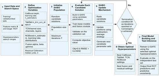
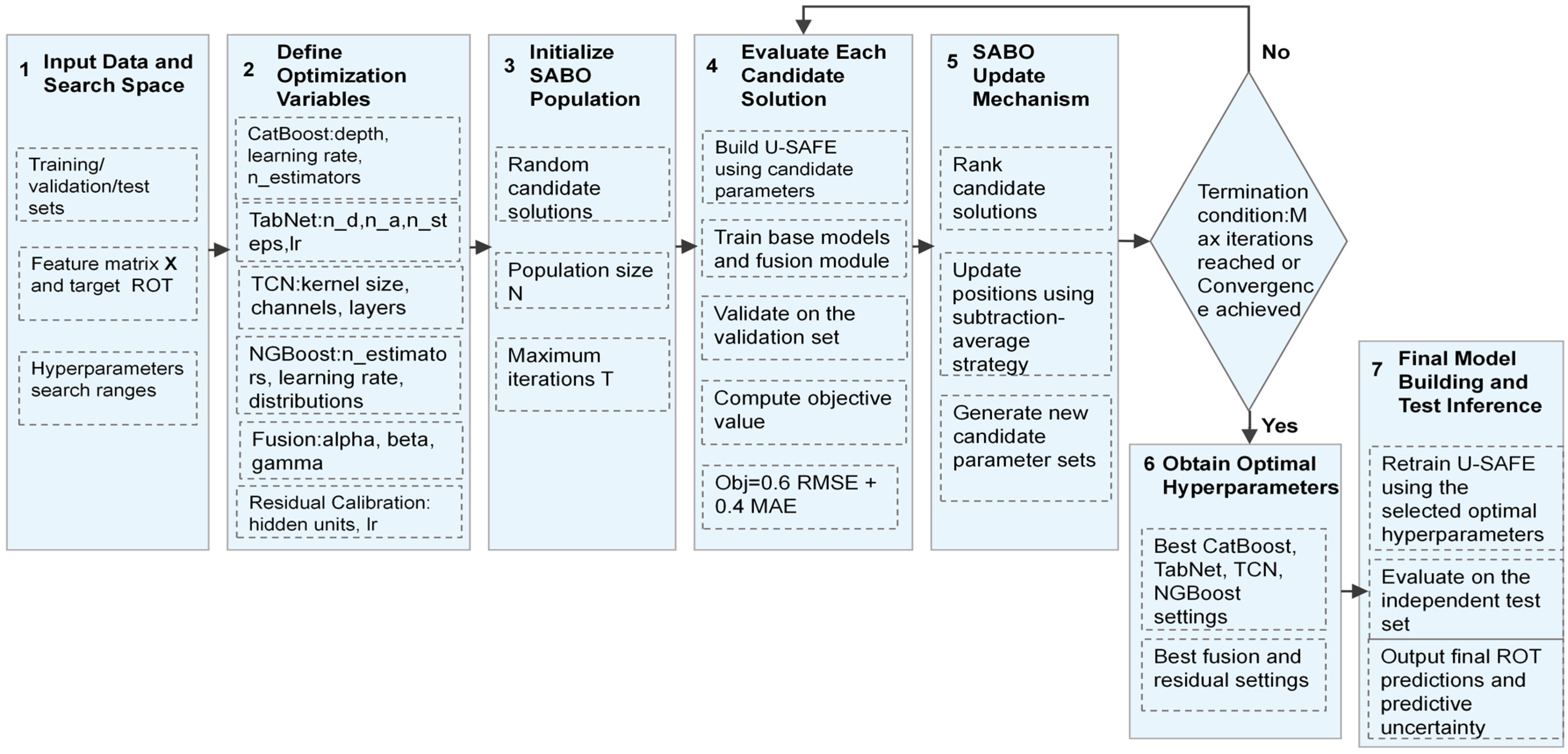
To improve the efficiency of hyperparameter search, this study employs the Subtraction-Average-Based Optimizer (SABO) for optimization of key model parameters. The optimized parameters include the network parameters of the expert models, the dynamic weighting coefficients, and the residual calibration network parameters. The overall SABO optimization procedure is illustrated in Figure 4.
Figure 4.
Flowchart of the SABO-assisted hyperparameter optimization.
4. Experimental Results and Analysis
All experiments in this study were implemented in Python 3.11 and conducted on a workstation equipped with an Intel Core i9 processor (Intel Corporation, Santa Clara, CA, USA), an NVIDIA GeForce RTX 4080 GPU (NVIDIA Corporation, Santa Clara, CA, USA) with 16 GB of graphics memory, and 64 GB of system RAM.
4.1. Data Preprocessing and Feature Construction
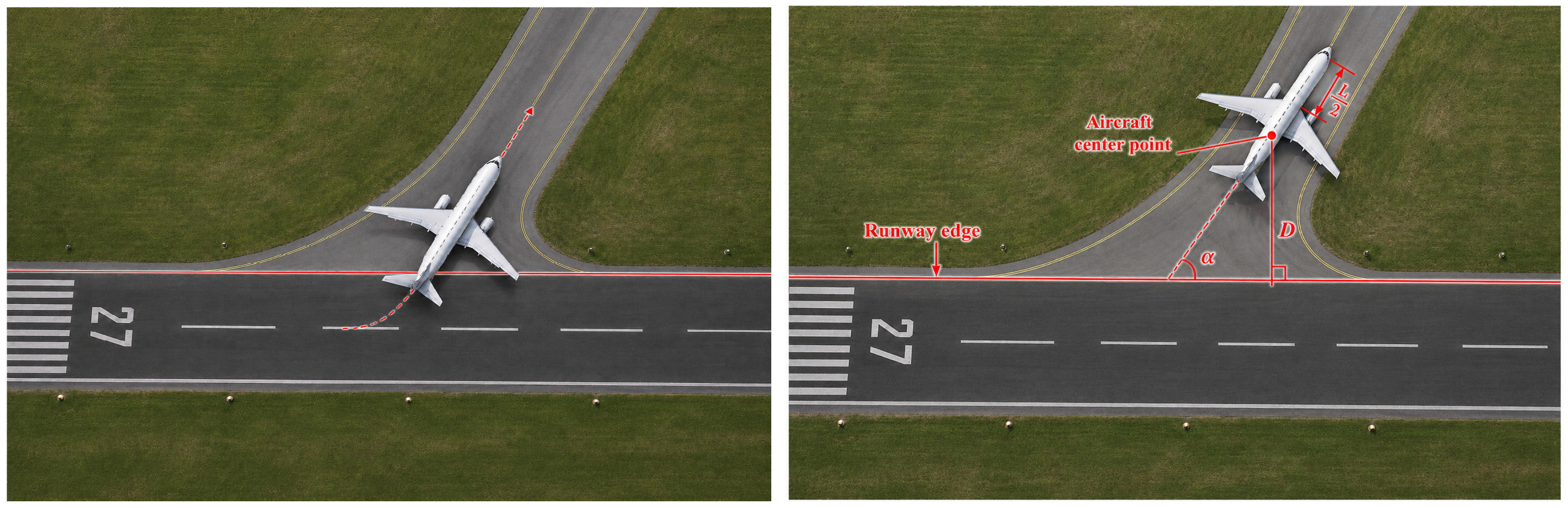
All experimental data were collected from the operational systems of Xi’an Xianyang Airport, Chengdu Tianfu Airport, and Guangzhou Baiyun Airport between February 2025 and May 2026. All three airports operate multi-runway systems with different geometric configurations and runway–taxiway layouts, and each system includes parallel runways. The dataset contains arrival operations on the commonly used landing runways, including 06R/24L and 05L/23R at Xi’an Xianyang International Airport, 01/19 and 02/20 at Chengdu Tianfu International Airport, and 01L/19R and 02R/20L at Guangzhou Baiyun International Airport. These primary arrival runways are equipped with multiple standard rapid-exit taxiways and perpendicular exit taxiways at different locations. Consequently, the three-airport dataset covers heterogeneous runway environments in terms of runway layout, runway-exit location, and touchdown-to-exit geometry. The multi-source data include ADS-B records, surface surveillance radar data, historical flight plan data, METAR meteorological data, available QAR data, and air traffic control operational records. In this study, runway occupancy time (ROT), measured in seconds, is defined as the time interval from the moment an aircraft crosses the runway threshold to the moment its tail completely vacates the runway. The ROT is calculated according to Equation (29), where denotes the threshold-crossing time of the (i)-th aircraft, and denotes the time at which its tail completely leaves the runway. These two timestamps are derived from surface surveillance data and aircraft GPS data. The first timestamp is determined by interpolating the flight trajectory and identifying the point closest to the runway threshold. The second timestamp is determined based on the minimum perpendicular distance from the runway boundary after the aircraft enters the exit taxiway. Since the GPS antenna used to record aircraft position is usually located near the aircraft center, the aircraft is considered to have vacated the runway when the perpendicular distance between its center and the runway boundary exceeds half of the aircraft projection length perpendicular to the runway axis, as illustrated in Figure 5.
Figure 5.
Calculation of aircraft runway exit time.
The collected raw data were first processed through trajectory matching and feature extraction. For missing values, continuous variables were handled using median imputation and linear interpolation, while missing categorical variables were assigned as “unknown”. For outlier processing, variables such as ROT and speed-related features were filtered according to reasonable aviation operational ranges. After removing abnormal samples and handling missing values, a total of 15,030 valid landing samples were obtained for model training and testing.
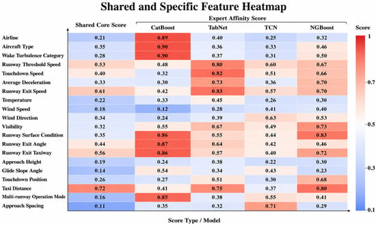
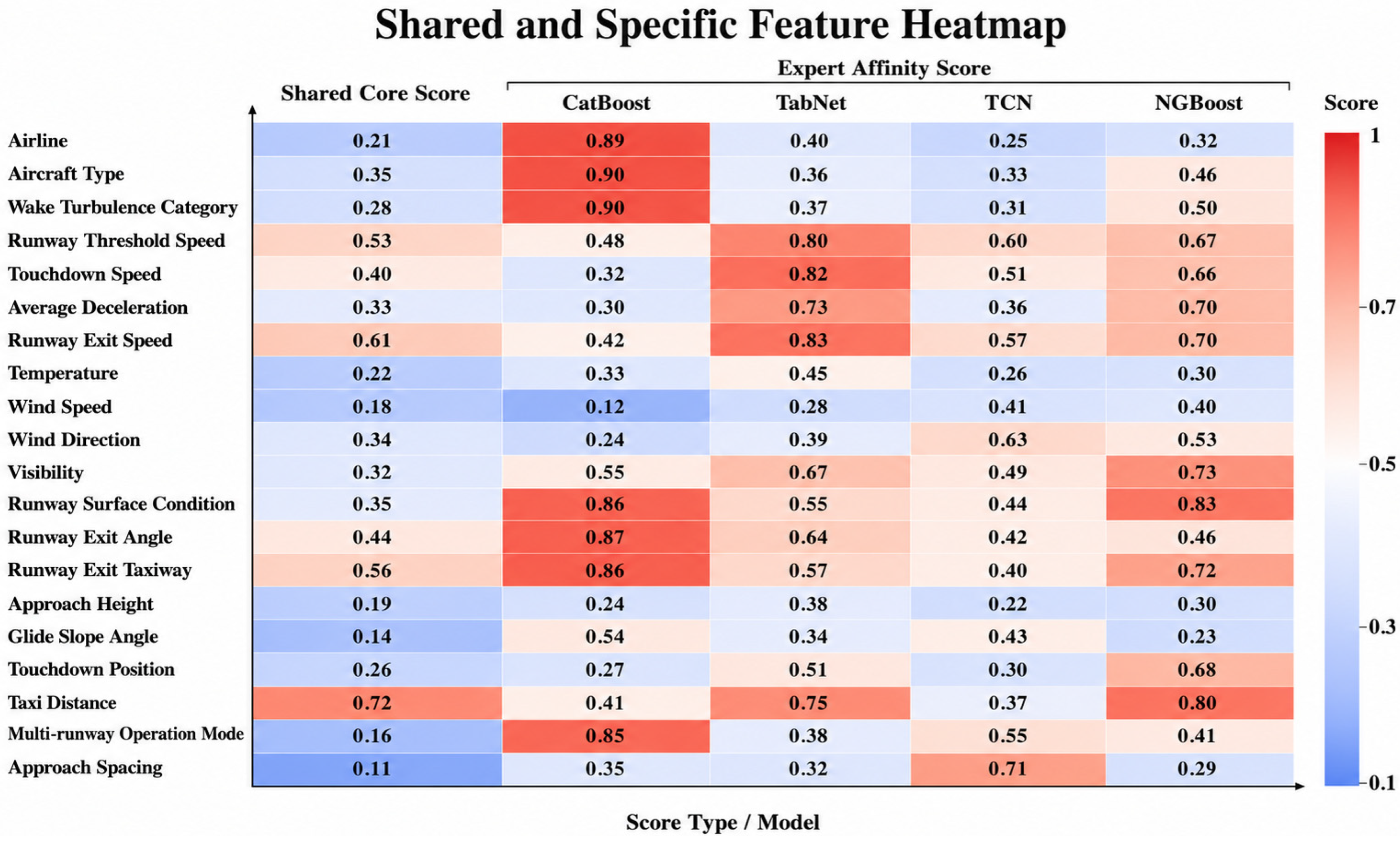
The valid samples were then preprocessed using feature-type-specific encoding strategies. Continuous, categorical, and directional features were encoded separately according to their data characteristics. After feature encoding, shared features and expert-specific features were selected, and the corresponding feature-score heatmaps are shown in Figure 6. Shared and expert-specific features were selected based on the cumulative score contribution ratio. For shared feature selection, features were ranked by the Shared Core Score and accumulated in descending order until the cumulative contribution ratio reached 80%. The selected features were used as shared inputs for all expert models, ensuring that the shared feature set retained the dominant global information. For expert-specific feature selection, the cumulative contribution threshold was set to 0.7 to preserve the most suitable features for each expert while reducing redundant inputs. The resulting shared and expert-specific feature sets are summarized in Table 2.
Figure 6.
Shared and Specific Features Heatmap.
Table 2.
Shared and Specific Features Table.
The constructed feature dataset was split in chronological order within each airport to avoid temporal information leakage caused by random partitioning. Specifically, the data were first grouped by airport and then divided chronologically within each airport, with the first 70% used for training, the middle 15% for validation, and the final 15% for testing. Since TCN is designed for temporal feature modeling, the historical sequence formed by the previous 20 landing samples, together with the current features, was used as its input. For a single runway at a large airport, the interval between two successive landing aircraft is typically about 2–3 min; therefore, using the previous 20 samples corresponds to an operational time span of approximately 40–60 min.
4.2. Model Parameters and Optimization Objectives
The overall framework adopts a SABO-based joint hyperparameter optimization strategy, in which the key hyperparameters of the heterogeneous expert models, the dynamic fusion layer, and the residual calibration network are optimized simultaneously. The initial values and search ranges of the main parameters in each module are listed in Table 3. The structural hyperparameters of AFG are not included in the SABO search space. Since AFG is a lightweight context-aware gating module for feature enhancement rather than the main prediction model, its structural parameters are fixed to default settings. Specifically, both the context embedding dimension and the gate hidden dimension are set to 32, the dropout rate is set to 0.1, and the internal weights are initialized using Xavier initialization and learned during model training. For SABO, the population size is set to 30, the maximum number of iterations is set to 50, and the early-stopping patience is set to 10, which provides a reasonable trade-off between global search capability and computational efficiency.
Table 3.
Hyperparameter Settings and Search Ranges of U-SAFE.
To balance prediction accuracy and error stability, a weighted combination of RMSE and MAE is used as the optimization objective of SABO. The weight coefficients were determined through a validation-based grid search. Specifically, the RMSE weight was searched from 0.1 to 0.9 with a step size of 0.1, and the MAE weight was set to . For each candidate weight pair, the model was optimized and evaluated on the validation set. The setting = 0.6 achieved the best trade-off between reducing large prediction errors and maintaining stable average accuracy. Therefore, the optimization objective is defined in Equation (30):
4.3. Overall Prediction Performance Comparison
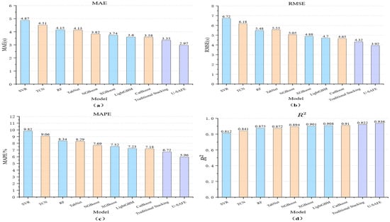
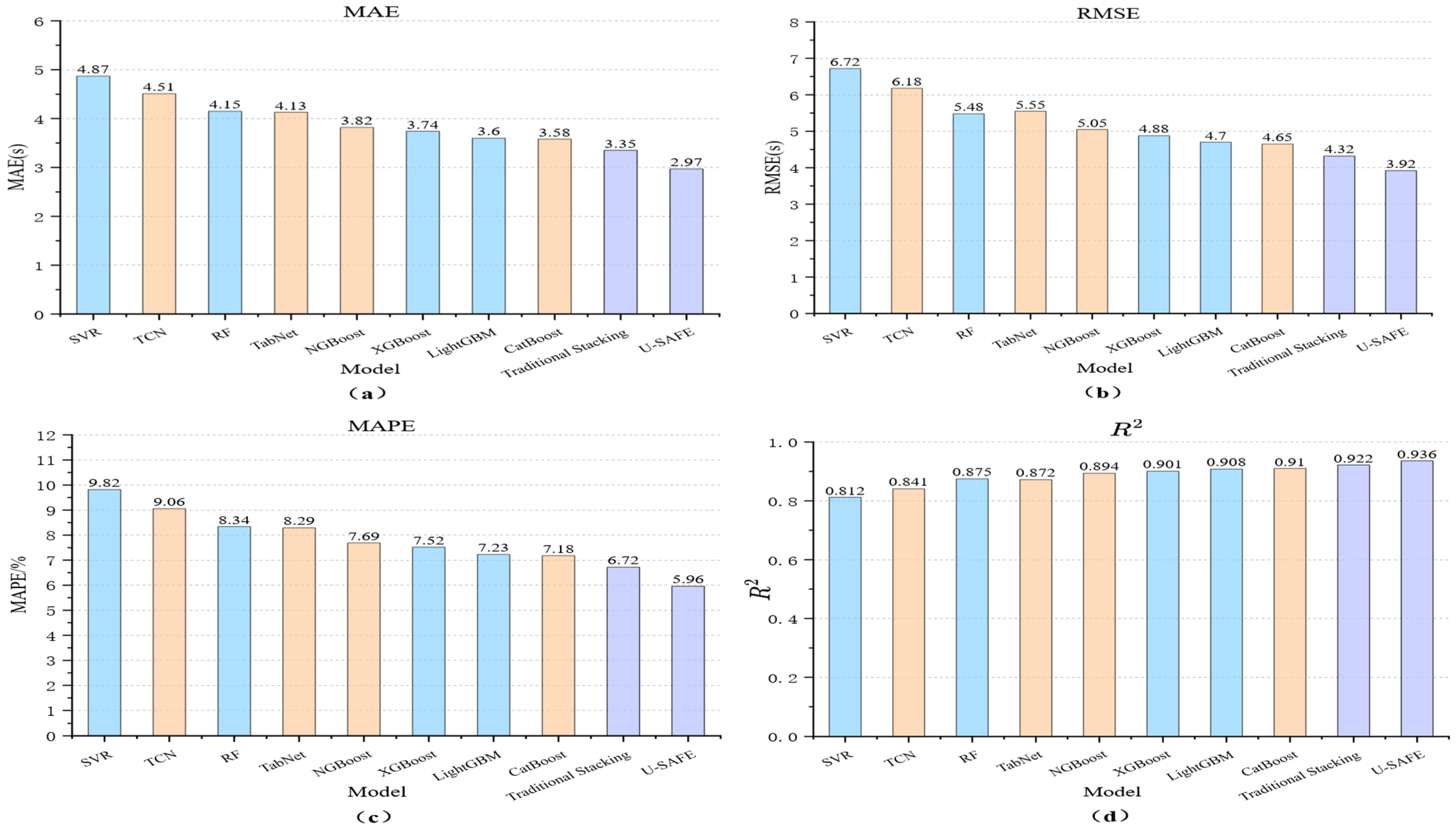
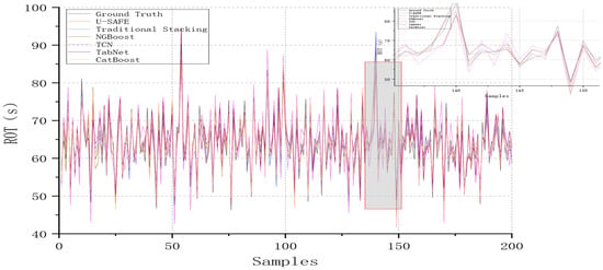
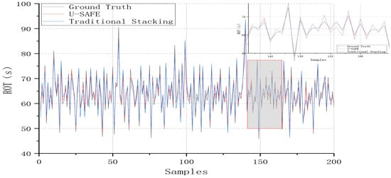
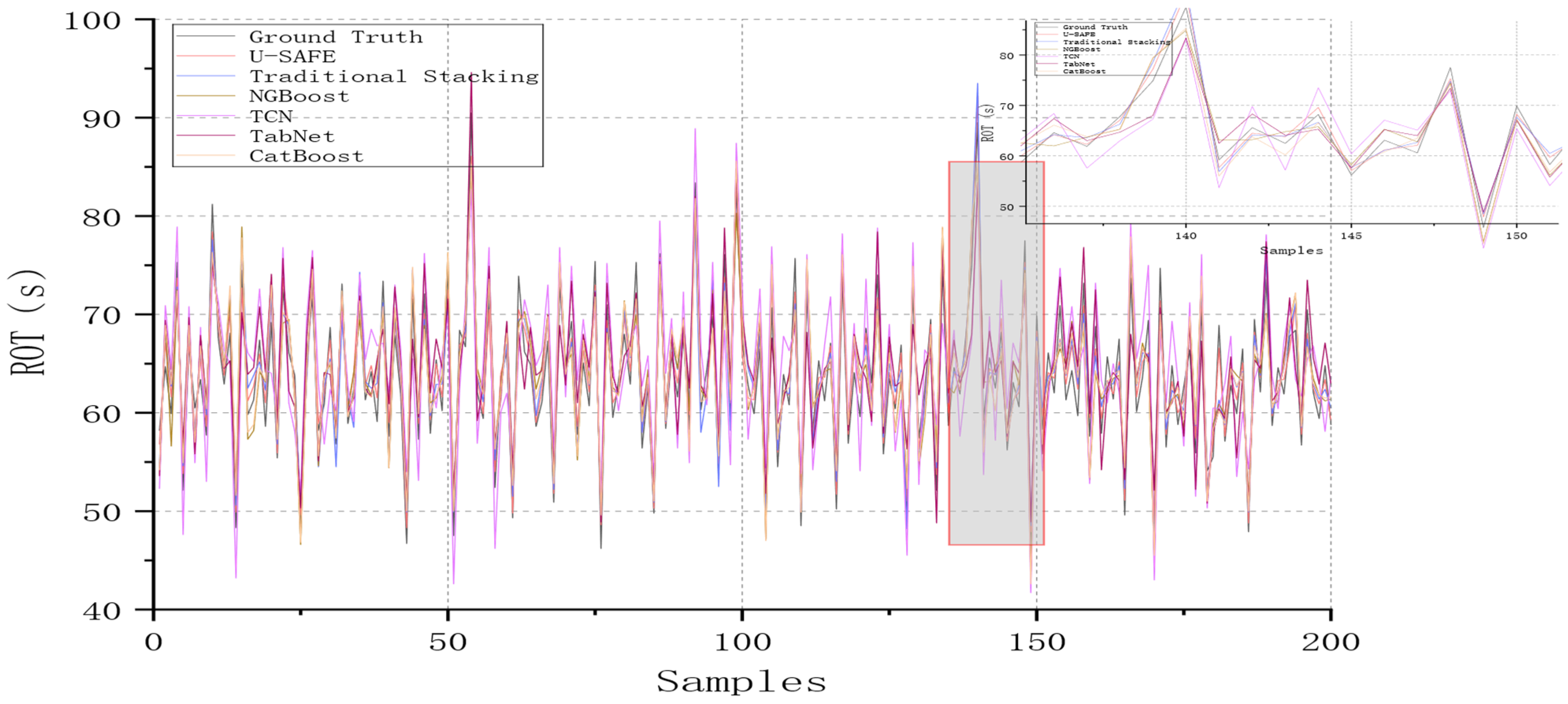
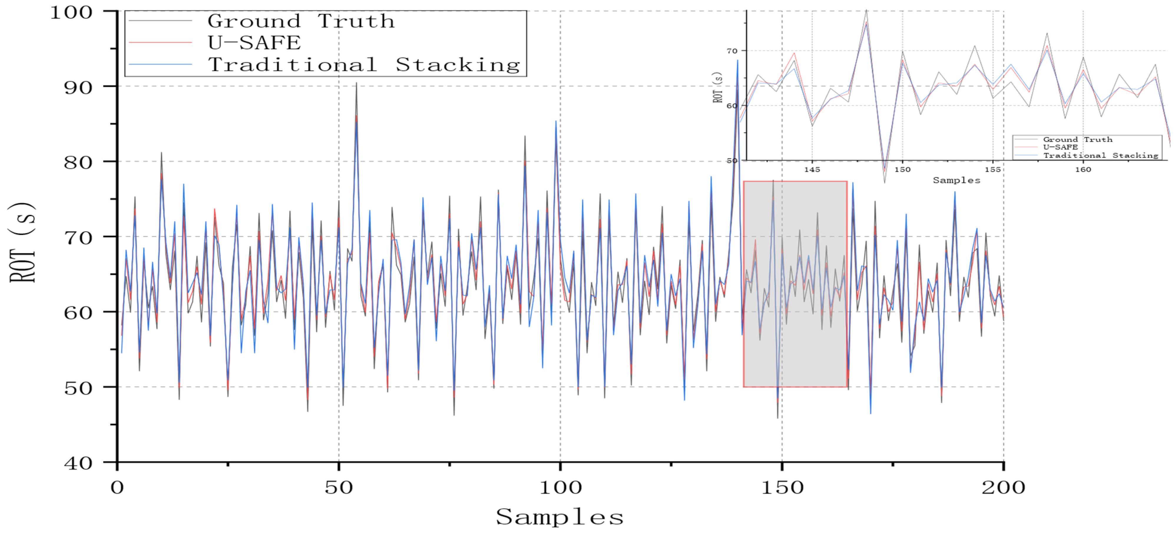
To evaluate the overall predictive performance of the U-SAFE framework, ten representative models were compared on the complete test set, including conventional models, heterogeneous base learners, traditional stacking, and the proposed U-SAFE model. Model performance was evaluated using four metrics: MAE, RMSE, MAPE, and , as shown in Figure 7. In addition, the prediction fitting results of different models on 200 randomly selected samples are presented in Figure 8.
Figure 7.
Overall prediction performance comparison of different models: (a) MAE; (b) RMSE; (c) MAPE; (d) .
Figure 8.
Comparison of ROT prediction performance with local zoom-in analysis.
Among the individual models, CatBoost and LightGBM achieve relatively better performance, indicating that tree-based boosting models have strong nonlinear modeling capability for multi-source heterogeneous tabular features. U-SAFE achieves the best performance among all compared models, with MAE, RMSE, and MAPE values of 2.97 s, 3.92 s, and 5.96%, respectively. Compared with Traditional Stacking, U-SAFE reduces MAE from 3.35 s to 2.97 s and RMSE from 4.32 s to 3.92 s, demonstrating that the proposed dynamic uncertainty-aware fusion mechanism and residual calibration module can further improve ROT prediction accuracy beyond conventional ensemble learning.
4.4. Fitting Performance and Error Distribution Analysis
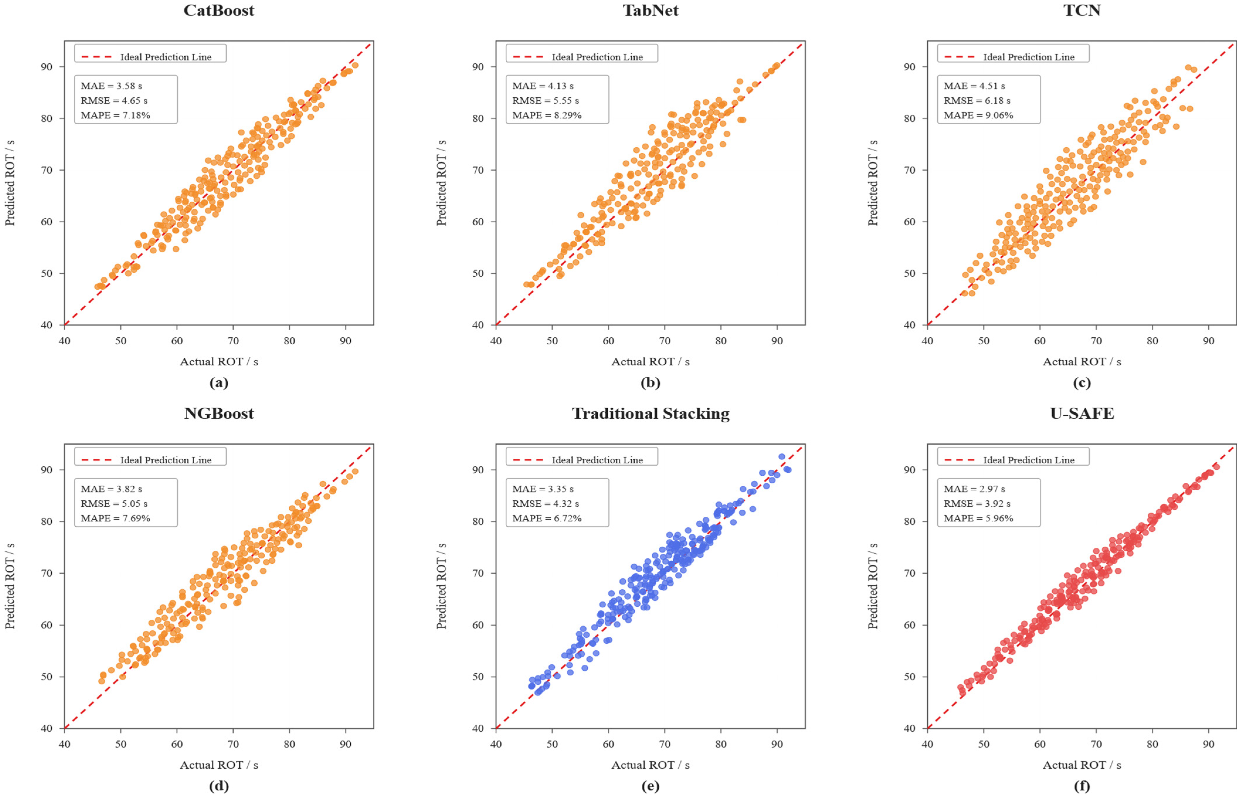
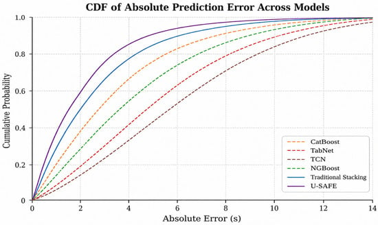
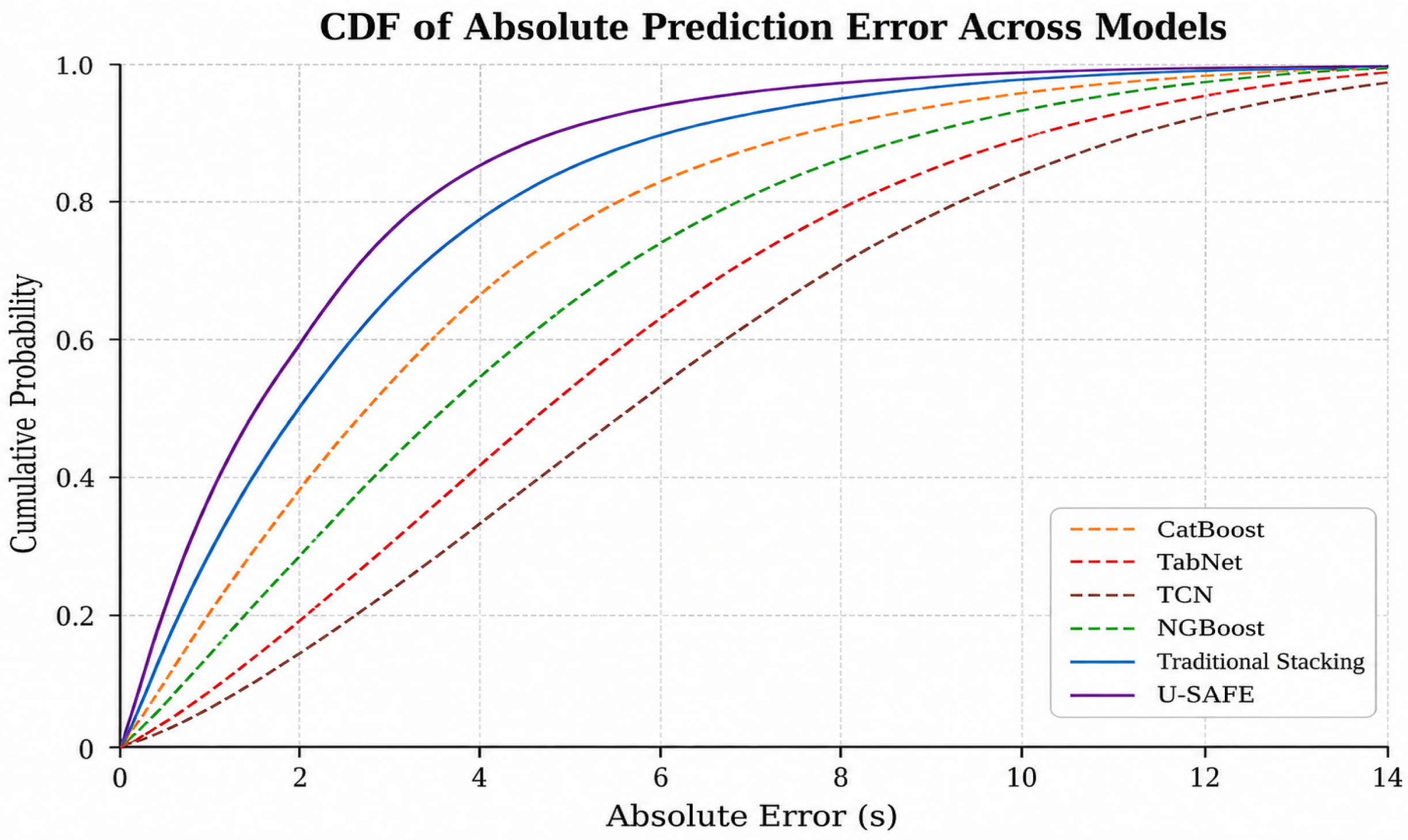
To further examine the fitting capability and error distribution characteristics of different models on ROT samples, observed-versus-predicted scatter plots and cumulative distribution function curves of absolute prediction errors were plotted for six representative models. As shown in Figure 9, the dispersion patterns differ markedly among the models. The prediction points of TCN and TabNet are relatively scattered, whereas CatBoost and NGBoost produce more concentrated distributions. Traditional Stacking further reduces prediction dispersion by integrating multiple base learners, but noticeable deviations remain for some high-ROT samples. In contrast, the prediction points of U-SAFE are most tightly distributed around the reference line, especially in the long-ROT range. This indicates that the proposed dynamic uncertainty-aware fusion and residual calibration mechanisms can effectively improve the fitting accuracy for complex and long-tail samples.
Figure 9.
Observed-versus-Predicted ROT scatter plots for six models: (a) CatBoost; (b) TabNet; (c) TCN; (d) NGBoost; (e) Traditional Stacking; (f) U-SAFE.
As shown in Figure 10, the CDF curve of U-SAFE consistently lies above those of the other models, indicating a higher sample coverage rate under the same absolute error threshold. In the small-error region, the U-SAFE curve rises more rapidly, suggesting that more samples are constrained within a smaller prediction error range. Meanwhile, U-SAFE maintains a higher cumulative probability in the medium-error region, demonstrating its stronger capability to suppress large prediction deviations.
Figure 10.
CDF of absolute prediction errors across different models.
4.5. Model Stability Analysis Under Repeated Seeds and Temporal Splits
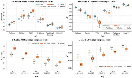
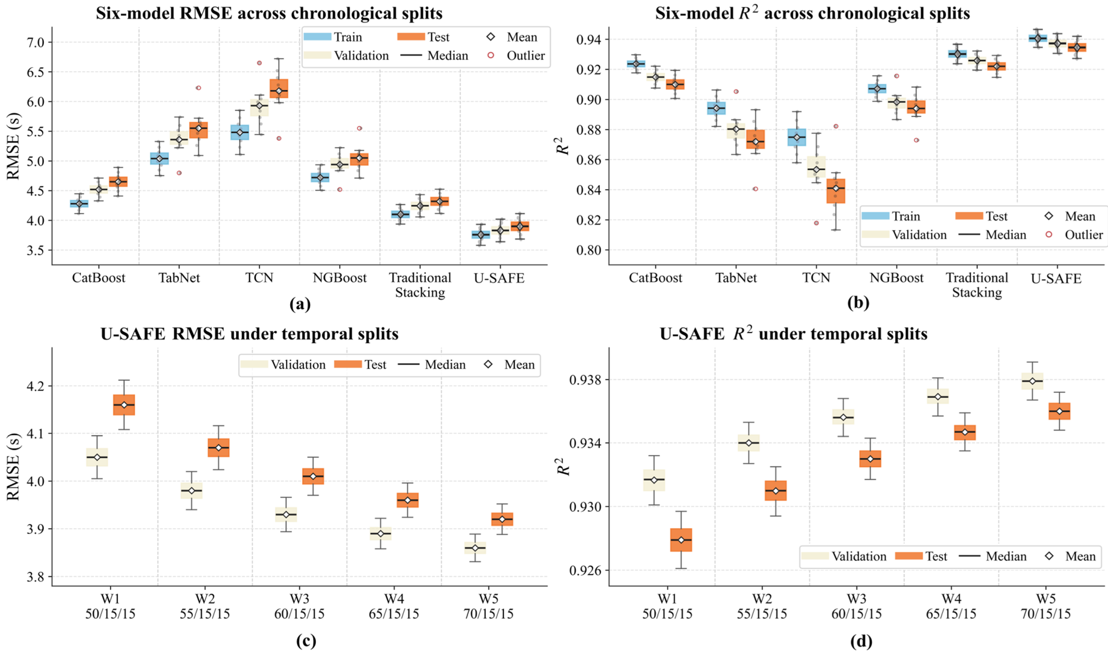
To further evaluate the training stability and temporal robustness of the models within the available observation period, repeated experiments with multiple random seeds were conducted. For Figure 11a,b, six representative models were trained under the same chronological 70%/15%/15% data split using ten different random seeds. The RMSE and distributions on the training, validation, and test sets were summarized using boxplots. The results show that U-SAFE achieves the lowest RMSE and the highest on the test set, while maintaining a compact distribution across different seeds. This indicates that the proposed framework not only improves prediction accuracy but also exhibits stable training behavior and consistent predictive performance on chronologically held-out samples. To assess temporal stability, five chronological temporal splits, denoted as W1–W5, were further constructed. The training proportions were gradually increased from 50% to 70%, while the validation and test proportions were both fixed at 15%. Under each temporal split, U-SAFE was independently trained using five random seeds, and the validation and test results were visualized in Figure 11c,d. As the training proportion increases, U-SAFE generally achieves lower RMSE and higher . In particular, W5 corresponds to the main 70%/15%/15% split and shows results consistent with the main experiment. These results indicate that U-SAFE maintains stable predictive performance across different chronological partitions within the available observation period and is not overly dependent on a specific temporal split. However, all W1–W5 partitions are constructed within the February 2025–May 2026 data-collection window and therefore do not constitute prospective validation on genuinely delayed data beyond the observation period. Long-term temporal generalization under future distribution shifts remains to be further evaluated using subsequently collected operational data.
Figure 11.
Model stability and generalization analysis under repeated seeds and temporal splits: (a) RMSE distributions of the six models on the training, validation, and test sets; (b) distributions of the six models on the training, validation, and test sets; (c) RMSE distributions of U-SAFE under five chronological temporal splits (W1–W5); (d) distributions of U-SAFE under five chronological temporal splits (W1–W5).
4.6. Airport-Specific Performance and Cross-Airport Generalization Analysis
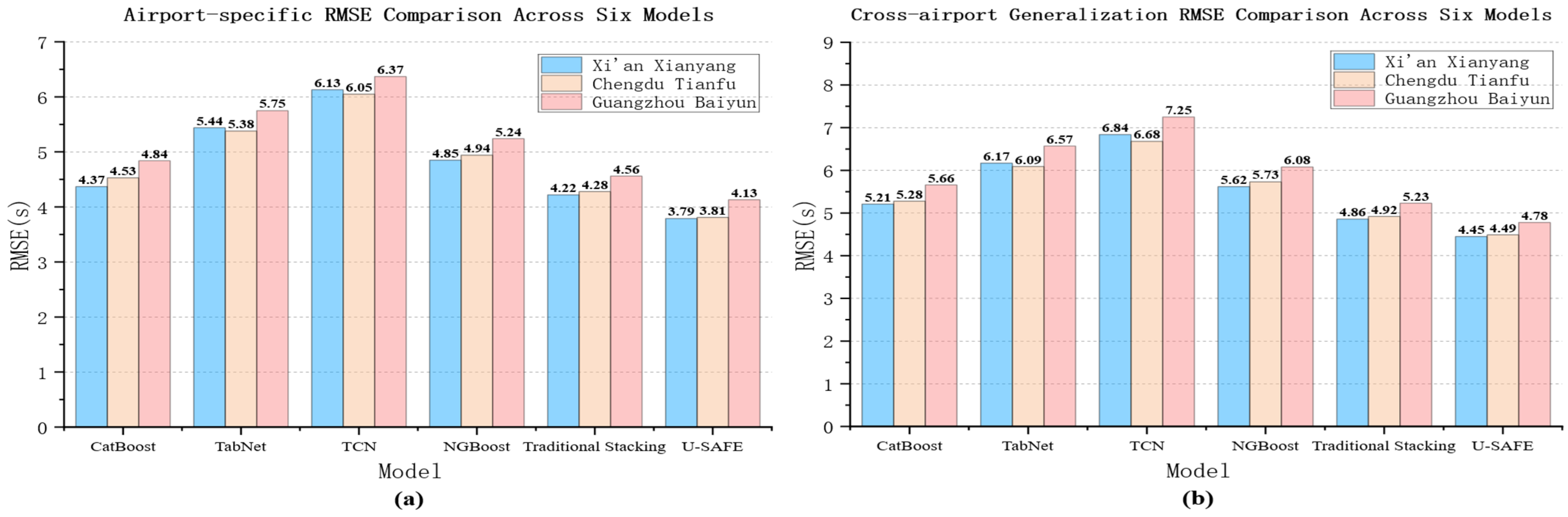
To evaluate the stability of the proposed model under different airport operating environments, airport-specific performance analysis and cross-airport generalization experiments were conducted. In the former, the models were jointly trained using data from the three airports, and their prediction performance was evaluated separately on each airport-specific test set. In the latter, a leave-one-airport-out strategy was adopted to assess the transferability of the models to unseen airports. RMSE was used as the evaluation metric in both experiments.
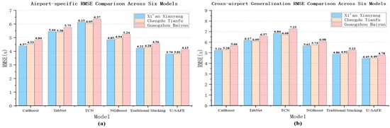
As shown in Figure 12a, U-SAFE achieves the lowest RMSE on all three airport-specific test sets, indicating that the proposed model can effectively adapt to differences in runway configurations, exit layouts, and operational conditions across airports. Overall, Guangzhou Baiyun Airport shows slightly higher prediction errors, suggesting greater operational complexity, whereas Xi’an Xianyang Airport exhibits relatively lower errors, indicating a more stable ROT sample distribution. As shown in Figure 12b, RMSE increases for all models in the leave-one-airport-out cross-airport tests, since the target airport is not included during training and differences in airport infrastructure and operational patterns increase the prediction difficulty. Nevertheless, U-SAFE consistently obtains the lowest RMSE across all cross-airport scenarios, demonstrating stronger cross-airport generalization capability.
Figure 12.
RMSE comparison across six models under different evaluation settings: (a) airport-specific RMSE comparison across Xi’an Xianyang, Chengdu Tianfu, and Guangzhou Baiyun airports; (b) cross-airport generalization RMSE comparison across the three airports.
4.7. Scenario-Based Robustness and Dynamic Fusion Analysis
To evaluate the predictive robustness of different models under complex airport operating conditions, four representative scenarios were considered: low visibility, thunderstorm, strong wind, and approach spacing control. These scenarios introduce typical disturbances to key operational features. All models were trained using the corresponding scenario-specific training sets and evaluated on the matching scenario-specific test subsets. As shown in Table 4, prediction errors generally increase under adverse conditions such as low visibility, thunderstorms, and strong winds. Nevertheless, U-SAFE achieves the lowest RMSE across all four complex scenarios. Its advantage is particularly evident under thunderstorm and low-visibility conditions, indicating that the proposed feature-aware and uncertainty-weighted dynamic fusion mechanism can adaptively adjust expert contributions according to changing operational conditions.
Table 4.
RMSE comparison under complex operating scenarios.
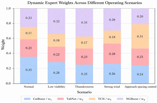
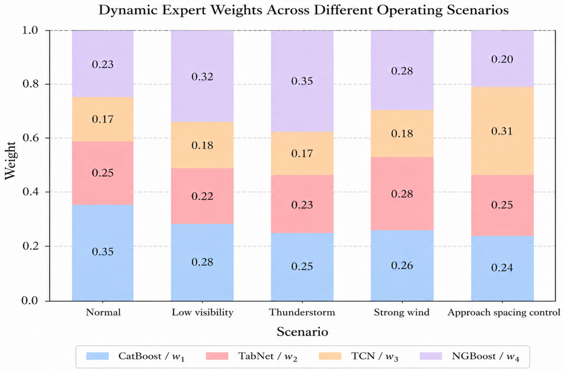
To examine the dynamic weight updating behavior of the base learners, the average fusion weights of the four expert models were calculated under different operating scenarios, as shown in Figure 13. The relative contribution of each expert varies across scenarios. Under normal operating conditions, CatBoost receives a relatively higher average weight, whereas the weight of NGBoost increases under low-visibility and thunderstorm conditions, and TCN receives a larger weight under approach-spacing-control scenarios. These variations should be interpreted as scenario-dependent predictive allocation rather than causal evidence that specific physical conditions directly activate particular experts. Since the fusion weights are jointly determined by predictive uncertainty, historical reliability, and scenario matching, the observed changes may reflect both differences in operational context and corresponding changes in the conditional uncertainty or error distribution of ROT. For example, the increased NGBoost weight during thunderstorms may partly reflect its relative predictive reliability under samples with greater uncertainty or heteroscedasticity. Therefore, Figure 13 illustrates adaptive expert allocation under observed operating conditions rather than causal identification of physical mechanisms.
Figure 13.
Dynamic expert weights across different operating scenarios.
In the U-SAFE framework, the fusion weights of the four base learners are not fixed global coefficients, but sample-specific weights adaptively computed by the dynamic fusion layer during inference. During training and validation, the four expert models are first trained, their historical reliability is estimated, and the control parameters of the dynamic fusion function are determined. Once training is completed, these parameters remain fixed during testing. For each input sample, the dynamic fusion layer calculates expert weights by jointly considering predictive uncertainty, historical reliability, and scenario matching degree. Experts with lower uncertainty, higher reliability, and stronger consistency with the current operational scenario are assigned larger weights. Therefore, U-SAFE can dynamically adjust expert contributions according to sample characteristics and operational contexts.
4.8. Probabilistic Prediction and Uncertainty Analysis
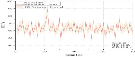
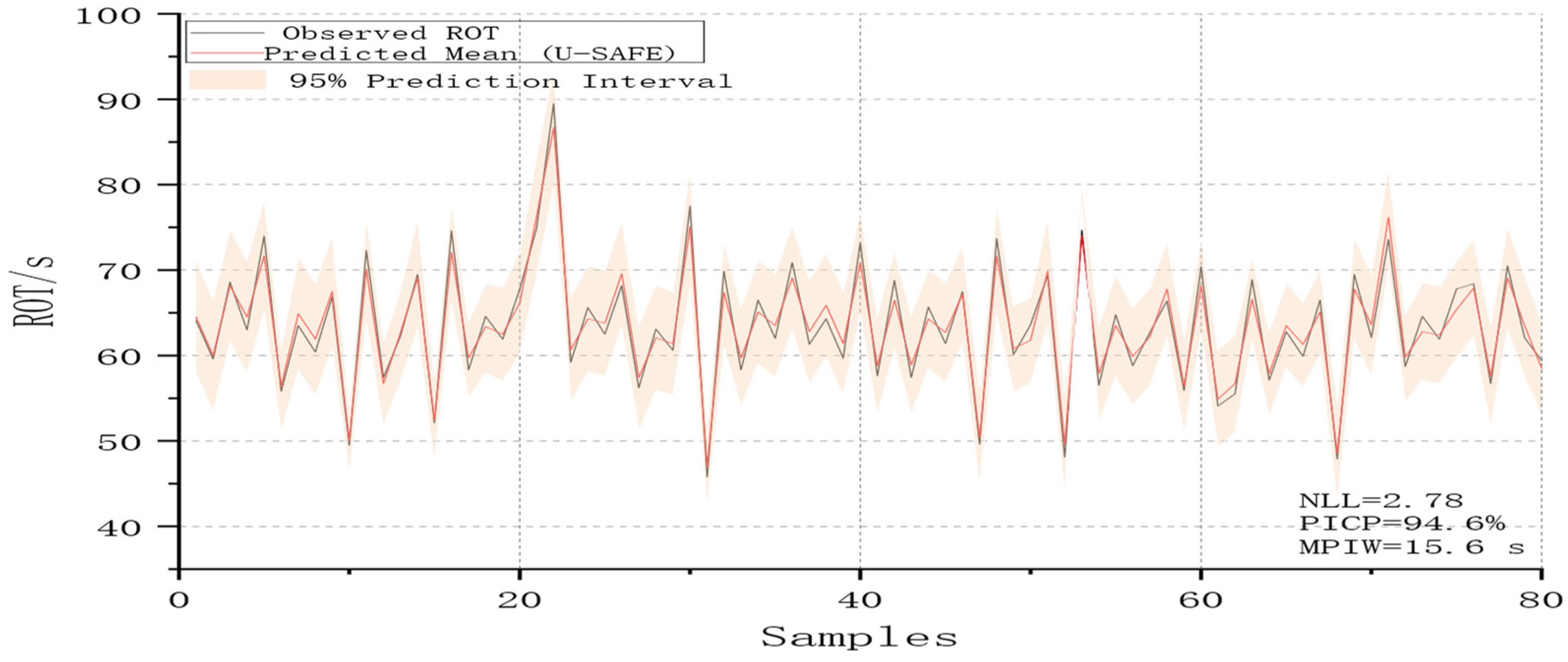
To evaluate the uncertainty estimation capability of the models, probabilistic prediction performance was compared using negative log-likelihood (NLL), prediction interval coverage probability (PICP), and mean prediction interval width (MPIW). Unlike deterministic error metrics, these indicators assess whether the predictive distribution can reasonably characterize the uncertainty in ROT prediction. A 95% prediction interval was adopted in this experiment. CatBoost was extended to probabilistic prediction through residual Gaussian calibration, NGBoost directly produced probabilistic outputs, and Traditional Stacking and U-SAFE constructed prediction intervals based on residual uncertainty. For U-SAFE, the predictive variance was estimated by combining expert-specific uncertainty, inter-expert prediction disagreement, and residual calibration variance. As shown in Table 5, U-SAFE achieves the lowest NLL among the four models, indicating that its predictive distribution is more consistent with the observed ROT values. In addition, U-SAFE obtains a PICP of 94.6%, which is closest to the nominal 95% confidence level, while maintaining an MPIW of only 15.6 s. This suggests that the proposed model can provide reliable uncertainty estimates without excessively widening the prediction intervals. Overall, U-SAFE achieves a better balance among prediction accuracy, interval reliability, and interval sharpness.
Table 5.
Probabilistic prediction performance comparison.
Figure 14 presents the prediction intervals of U-SAFE on 80 representative test samples. The black curve denotes the observed ROT, the red curve represents the predicted mean, and the shaded region indicates the 95% prediction interval. Most observations fall within the prediction interval, while the interval width increases moderately for high-ROT or complex samples. This demonstrates the adaptive uncertainty characterization capability of the proposed model.
Figure 14.
Predictive intervals of U-SAFE on test samples.
4.9. Optimization Effectiveness Analysis and Ablation Study
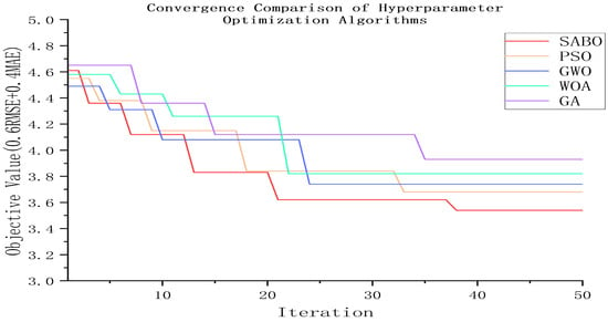
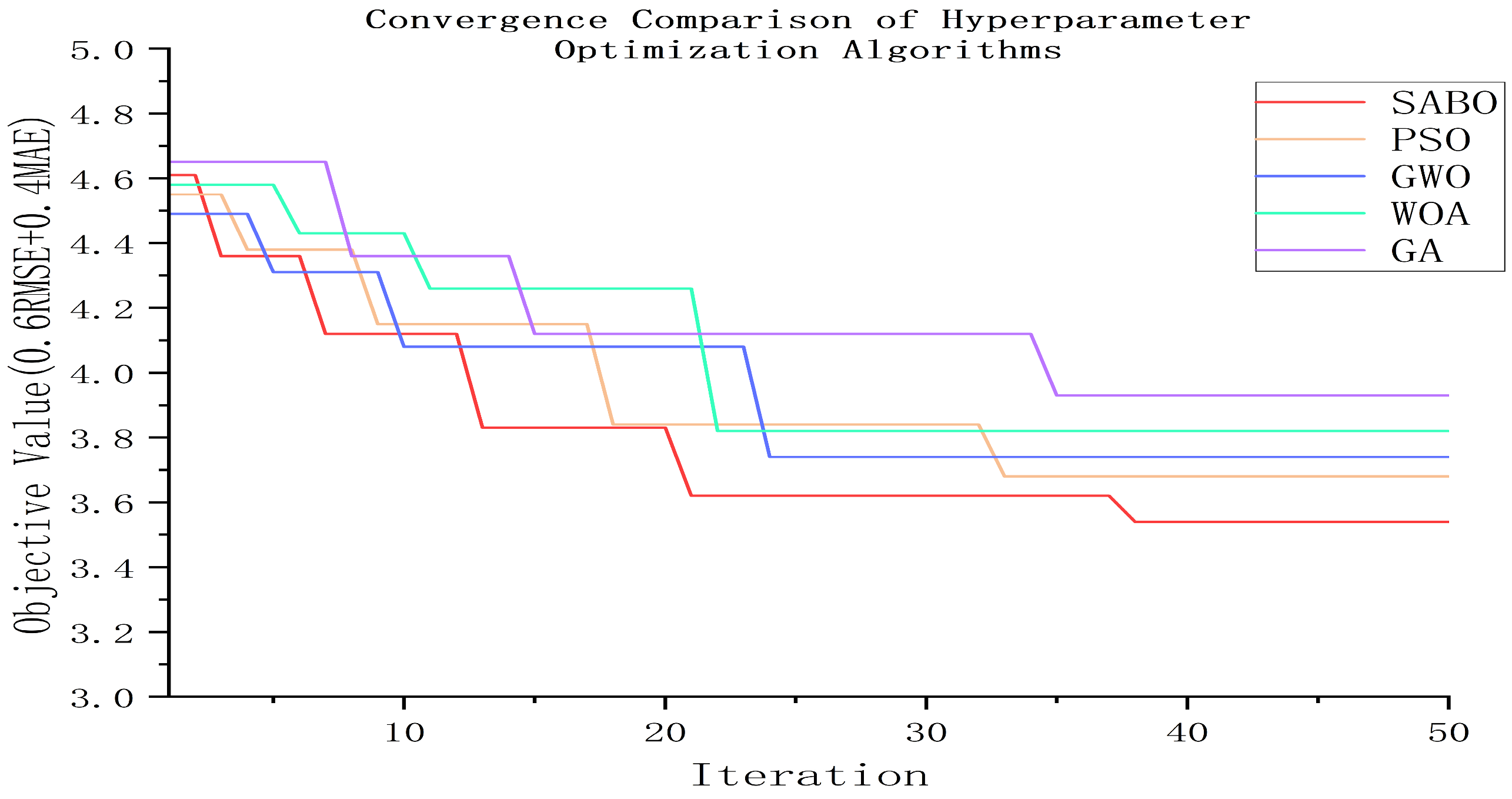
To further evaluate the optimization effectiveness of SABO, its convergence performance was compared with several commonly used hyperparameter optimization algorithms, as shown in Figure 15. SABO achieves a lower validation objective value within a limited number of iterations and exhibits a stable convergence trend, indicating its effectiveness in searching the hyperparameter space of the U-SAFE framework under a moderate computational budget.
Figure 15.
Convergence comparison of hyperparameter optimization algorithms.
To verify the effectiveness of the key modules in the proposed framework, ablation experiments were conducted, as shown in Table 6. In addition to the module-removal variants, a reduced U-SAFE configuration retaining only CatBoost and TCN was evaluated using the same dynamic weighting principle to examine the effect of reducing expert diversity. The reduced configuration achieves an MAE of 3.05 s, an RMSE of 4.04 s, a MAPE of 6.20%, and an of 0.932, while the full U-SAFE achieves 2.97 s, 3.92 s, 5.96%, and 0.936, respectively. These results indicate that the reduced two-expert configuration remains competitive, whereas the inclusion of TabNet and NGBoost provides a modest but consistent improvement, reflecting a trade-off between predictive performance and model complexity. Among the remaining ablation variants, removing the dynamic expert fusion mechanism leads to a clear increase in prediction error, indicating that fixed or static ensemble weights cannot effectively adapt to changes in expert contributions under different operating scenarios. Removing the uncertainty-aware weighting term increases RMSE, suggesting that uncertainty information helps suppress large errors in complex samples. In addition, the performance degradation after removing the residual calibration module demonstrates its effectiveness in correcting systematic bias after fusion. The model without SABO optimization also shows higher errors, confirming that the proposed hyperparameter optimization strategy contributes positively to overall prediction performance.
Table 6.
Ablation Study Table.
5. Conclusions
This paper proposes U-SAFE, an uncertainty-aware scenario-adaptive feature ensemble learning framework for aircraft landing runway occupancy time prediction. By integrating shared-specific feature assignment, adaptive feature gating, heterogeneous expert modeling, dynamic uncertainty-aware fusion, and residual calibration, the proposed framework effectively captures the complex relationships between ROT and multi-source factors, including aircraft performance, speed states, runway exits, meteorological conditions, and operational spacing. Experiments on 15,030 valid landing samples from Xi’an Xianyang, Chengdu Tianfu, and Guangzhou Baiyun airports demonstrate that U-SAFE achieves the best overall performance, with MAE, RMSE, and MAPE values of 2.97 s, 3.92 s, and 5.96%, respectively. It outperforms conventional models, individual base learners, and traditional stacking. Fitting performance and error distribution analyses further show that U-SAFE can more effectively reduce prediction deviations for long-ROT and fluctuation-prone samples. Airport-specific testing, cross-airport generalization, and complex-scenario experiments confirm the stability and robustness of the proposed framework. U-SAFE maintains lower errors across different airport test sets and under challenging conditions such as low visibility, thunderstorms, strong winds, and approach spacing control. This indicates that its dynamic expert fusion mechanism can adaptively adjust expert contributions according to changing operational contexts. Uncertainty analysis shows that U-SAFE achieves an NLL of 2.78, a PICP of 94.6%, and an MPIW of 15.6 s, providing compact prediction intervals while maintaining reliable coverage. Ablation results verify the positive contributions of shared-specific feature assignment, adaptive feature gating, dynamic expert fusion, uncertainty-aware weighting, residual calibration, and SABO-based hyperparameter optimization. Overall, U-SAFE provides an effective solution for accurate ROT prediction and uncertainty-aware decision-making in complex airport operating environments. The framework is intended to support safety-aware runway operations rather than to promote reductions in ROT at the expense of established safety requirements and standard operating procedures.
The findings of this study should nevertheless be interpreted in light of several limitations. First, although the present study considers runway-exit, touchdown-position, taxi-distance, and runway-operating-mode information, complete airport-topology attributes, including the full taxiway network, apron configuration, aircraft-stand distribution, and terminal layout, are not explicitly represented; therefore, their indirect effects on ROT cannot be separately quantified. Second, human-related operational factors, such as flight-crew workload, operational behavior, and controller decision-making, are not explicitly represented in the current dataset. Third, although cross-airport and chronological-split experiments were conducted, the dataset is limited to three Chinese airports within the February 2025–May 2026 observation window. Consequently, generalization to additional airports and long-term robustness under future temporal distribution shifts require further prospective validation. Fourth, the scenario-dependent expert weights represent conditional predictive adaptations rather than causal effects of individual operational factors. Finally, end-to-end inference latency under operational tower conditions has not yet been systematically benchmarked, and the online historical-neighbor retrieval introduces additional computational overhead. Future work will therefore focus on broader multi-airport and prospective temporal validation, richer airport-topology and human-related information, lightweight neighbor-retrieval strategies, and systematic real-time deployment evaluation.
Author Contributions
Conceptualization, M.Z. and Z.Y.; methodology, M.Z.; software, Z.W.; validation, M.Z., Z.W. and Z.Y.; formal analysis, M.Z.; investigation, M.Z.; resources, Z.W.; data curation, Z.W.; writing—original draft preparation, M.Z.; writing—review and editing, Q.C.; visualization, Z.W.; supervision, Q.C.; project administration, Q.C.; funding acquisition, Q.C. All authors have read and agreed to the published version of the manuscript.
Funding
This research was funded by the Transportation Research Project of the Department of Transport of Shaanxi Province, China, under the project “Air–Ground Collaborative Control Methods and Applications for Airports under Complex Situations” (Project No. 25-53K). The APC was funded by Xidian University.
Data Availability Statement
The datasets used and analyzed in this study are not publicly available due to confidentiality restrictions and data use agreements with the Air Traffic Management Bureau of the Civil Aviation Administration of China. The datasets contain safety-sensitive operational information, including ADS-B, MLAT, air traffic control system records, flight trajectory data, and airborne QAR data. Processed data and statistical results supporting the findings of this study may be available from the corresponding author upon reasonable request, subject to approval from the relevant data providers.
Acknowledgments
The authors declare that no generative AI technologies were used in the preparation of this manuscript.
Conflicts of Interest
The authors declare no conflicts of interest.
Abbreviations
The following abbreviations are used in this manuscript:
| ROT | Runway Occupation Time |
| TCN | Temporal Convolutional Network |
| QAR | Quick Access Recorder |
| ADS-B | Automatic Dependent Surveillance–Broadcast |
| METAR | Meteorological Terminal Aviation Routine Weather Report |
| ICAO | International Civil Aviation Organization |
| RMSE | Root Mean Squared Error |
| MAE | Mean Absolute Error |
| MAPE | Mean Absolute Percentage Error |
| Coefficient of Determination |
References
- EUROCONTROL. Optimised Runway Occupancy Time Spacings for Arrivals (“ROCAT” Solution); Version 1.1; EUROCONTROL: Brussels, Belgium, 2025; Available online: https://www.eurocontrol.int/publication/optimised-runway-occupancy-time-spacings-arrivals (accessed on 30 December 2025).
- EUROCONTROL. Enhancing Airside Capacity: The Complete Guide, 2nd ed.; EUROCONTROL: Brussels, Belgium, 2003. [Google Scholar]
- Barbaresco, F.; Juge, P.; Klein, M.; Ricci, Y.; Schneider, J.-Y.; Moneuse, J.-F. Optimising runway throughput through wake vortex detection, prediction and decision support tools. In Proceedings of the 2011 Tyrrhenian International Workshop on Digital Communications—Enhanced Surveillance of Aircraft and Vehicles (TIWDC/ESAV), Capri, Italy, 12–14 September 2011; pp. 27–32. [Google Scholar]
- International Civil Aviation Organization (ICAO). Procedures for Air Navigation Services—Air Traffic Management (PANS-ATM), Doc 4444, 16th ed.; ICAO: Montreal, QC, Canada, 2016. [Google Scholar]
- EUROCONTROL. RWY Throughput Enhancement Solutions by EUROCONTROL. In Proceedings of the 2025 Capacity Assessment Workshop. 2025. Available online: https://www.icao.int/sites/default/files/APAC/Meetings/2025/2025%20Capacity%20Assessment%20WS/Day%202/SP-11-RWY-Throughput-Enahncement-Solutions-by-EUROCONTROL.pdf (accessed on 30 December 2025).
- Hu, J.Q.; Mirmohammadsadeghi, N.; Trani, A.A. Runway occupancy time constraint and runway throughput estimation under reduced arrival wake separation rules. In Proceedings of the AIAA Aviation 2019 Forum, Dallas, TX, USA, 17–21 June 2019. AIAA 2019-3046. [Google Scholar] [CrossRef] [Scilit]
- Pérez Maroto, M.; Serrano-Mira, L.; Ayra, E.S.; Pérez-Castán, J.A.; Gómez Arnaldo, C.; Pérez Sanz, L. Analysis of the Relationship Between Runway Occupancy Time (ROT) and Aircraft Separation on Final Approach as a Constraint on Runway Capacity Under High-Demand Operations. Aerospace 2026, 13, 56. [Google Scholar] [CrossRef] [Scilit]
- Martinez, J.C.; Trani, A.A.; Ioannou, P.G. Modeling airside airport operations using general-purpose, activity-based, discrete-event simulation tools. Transp. Res. Rec. 2001, 1744, 65–71. [Google Scholar] [CrossRef] [Scilit]
- Kolos-Lakatos, T. The Influence of Runway Occupancy Time and Wake Vortex Separation Requirements on Runway Throughput. Master’s Thesis, Massachusetts Institute of Technology, Cambridge, MA, USA, 2013. [Google Scholar]
- Kumar, V.; Sherry, L.; Kicinger, R. Runway occupancy time extraction and analysis using surface track data. In Proceedings of the 89th Annual Meeting of the Transportation Research Board, Washington, DC, USA, 10–14 January 2010. [Google Scholar]
- Meijers, N.P.; Hansman, R.J. A data-driven approach to understanding runway occupancy time. In Proceedings of the AIAA Aviation 2019 Forum, Dallas, TX, USA, 17–21 June 2019. AIAA 2019-3045. [Google Scholar] [CrossRef] [Scilit]
- Herrema, F.F.; Curran, R.; Visser, H.G.; Treve, V.; Desart, B. Predicting abnormal runway occupancy times and observing related precursors. J. Aerosp. Inf. Syst. 2018, 15, 10–21. [Google Scholar] [CrossRef] [Scilit]
- Nikoleris, T.; Hansen, M. Effect of trajectory prediction and stochastic runway occupancy times on aircraft delays. Transp. Sci. 2015, 50, 110–119. [Google Scholar] [CrossRef] [Scilit]
- Dönmez, K. Aircraft sequencing under the uncertainty of the runway occupancy times of arrivals during the backtrack procedure. Aeronaut. J. 2023, 127, 562–580. [Google Scholar] [CrossRef] [Scilit]
- Skorupski, J.; Wierzbicki, H. Airport Capacity Increase via the Use of Braking Profiles. Transp. Res. Part C Emerg. Technol. 2017, 80, 467–484. [Google Scholar] [CrossRef] [Scilit]
- Sherali, H.D.; Hobeika, A.G.; Trani, A.A.; Kim, B.J. An Integrated Simulation and Dynamic Programming Approach for Determining Optimal Runway Exit Locations. Manag. Sci. 1992, 38, 1049–1062. [Google Scholar] [CrossRef] [Scilit]
- Maltinti, F.; Flore, M.; Pigozzi, F.; Coni, M. Optimizing Airport Runway Capacity and Sustainability through the Introduction of Rapid Exit Taxiways: A Case Study. Sustainability 2024, 16, 5359. [Google Scholar] [CrossRef] [Scilit]
- Kim, M.; Baik, H.; Choi, D.; Shin, J. Impact Analysis of Rapid Exit Taxiways on Runway Occupancy Time. J. Korean Soc. Aviat. Aeronaut. 2025, 33, 193–203. [Google Scholar] [CrossRef] [Scilit]
- Chow, H.W.; Lim, Z.J.; Alam, S. Data-driven runway occupancy time prediction using decision trees. In Proceedings of the 2021 IEEE/AIAA 40th Digital Avionics Systems Conference (DASC), San Antonio, TX, USA, 3–7 October 2021; pp. 1–9. [Google Scholar] [CrossRef] [Scilit]
- Meijers, N.P. Data-Driven Predictive Analytics of Runway Occupancy Time for Improved Capacity at Airports. Master’s Thesis, Massachusetts Institute of Technology, Cambridge, MA, USA, 2019. [Google Scholar]
- Mirmohammadsadeghi, N.; Trani, A.A. Enhancements to the runway exit design interactive model using a hybrid simulation approach for estimating runway occupancy times at airports. In Proceedings of the AIAA Scitech 2020 Forum, Orlando, FL, USA, 6–10 January 2020; AIAA 2020-1403, pp. 1–10. [Google Scholar] [CrossRef] [Scilit]
- Spencer, T.L.; Trani, A.A. Predictive models of departure and arrival occupancy time and takeoff distance. J. Air Transp. 2019, 27, 81–95. [Google Scholar] [CrossRef] [Scilit]
- Herrema, F.; Curran, R.; Hartjes, S.; Ellejmi, M.; Bancroft, S.; Schultz, M. A machine learning model to predict runway exit at Vienna Airport. Transp. Res. Part E Logist. Transp. Rev. 2019, 131, 329–342. [Google Scholar] [CrossRef] [Scilit]
- Xing, Z.; Jiang, S.; Luo, Q.; Luo, X. Prediction of flight taxi-out time in a busy airport based on LWSVR. J. Syst. Simul. 2020, 32, 927–935. [Google Scholar] [CrossRef]
- Lim, Z.J.; Goh, S.K.; Dhief, I.; Alam, S. Causal effects of landing parameters on runway occupancy time using causal machine learning models. In Proceedings of the 2020 IEEE Symposium Series on Computational Intelligence (SSCI), Canberra, ACT, Australia, 1–4 December 2020; pp. 2713–2722. [Google Scholar] [CrossRef] [Scilit]
- Li, N.; Fu, R. Research on runway occupation time prediction of approaching aircrafts. Sci. Technol. Eng. 2023, 23, 11437–11444. [Google Scholar] [CrossRef]
- Pan, W.J.; Zhang, H.H.; Liu, T.; Wu, T.Y.; Yin, Z.R. Runway occupancy time prediction based on neural network. J. Command Control 2022, 8, 214–220. [Google Scholar] [CrossRef]
- Chen, Y.; Li, Y.; Zhao, R.; Gao, H. Prediction of aircraft landing runway occupation time based on SSA-CNN. Sci. Technol. Eng. 2024, 24, 2813–2820. [Google Scholar] [CrossRef]
- Nguyen, A.-D.; Pham, D.-T.; Lilith, N.; Alam, S. Model generalization in arrival runway occupancy time prediction by feature equivalences. arXiv 2022, arXiv:2201.11654. [Google Scholar] [CrossRef] [Scilit]
- Dai, L.; Hansen, M. Real-time prediction of runway occupancy buffers. In Proceedings of the 2020 International Conference on Artificial Intelligence and Data Analytics for Air Transportation (AIDA-AT), Singapore, 3–4 February 2020; pp. 1–11. [Google Scholar] [CrossRef] [Scilit]
- Hänggi, K.; Waltert, M.; Wilde, J. Prediction of arrival runway occupancy time and exit taxiway using ADS-B trajectories. J. Open Aviat. Sci. 2026, 4. [Google Scholar] [CrossRef] [Scilit]
- Gao, H.; Xie, Y.; Yuan, C.; He, X.; Niu, T. Prediction of aircraft arrival runway occupancy time based on machine learning. Int. J. Comput. Intell. Syst. 2023, 16, 150. [Google Scholar] [CrossRef] [Scilit]
- Martínez, D.; Belkoura, S.; Cristóbal, S.; Herrema, F.; Wächter, P. A boosted tree framework for runway occupancy and exit prediction. In Proceedings of the Eighth SESAR Innovation Days, Salzburg, Austria, 3–7 December 2018; Available online: https://www.sesarju.eu/sites/default/files/documents/sid/2018/papers/SIDs_2018_paper_51.pdf (accessed on 5 December 2025).
- Mirmohammadsadeghi, N.; Trani, A.A. Prediction of Runway Occupancy Time and Runway Exit Distance with Feedforward Neural Networks. In Proceedings of the AIAA Scitech 2020 Forum, Orlando, FL, USA, 6–10 January 2020. AIAA 2020-1402. [Google Scholar] [CrossRef] [Scilit]
- Porcayo, A.; Pang, Y.; Thomas, M.; Clarke, J.-P. Data-Driven Runway and Taxiway Exits Prediction of Landing Aircraft: A Case Study at Hartsfield–Jackson Atlanta International Airport. J. Air Transp. Manag. 2026, 136, 103063. [Google Scholar] [CrossRef] [Scilit]
- Huang, Z.; Yue, Z.; Tang, W.; Wang, T.; Zhang, X. A TCN-FEP hybrid model with multi-scale feature interaction network for departure runway occupation time prediction. Aerospace 2026, 13, 510. [Google Scholar] [CrossRef] [Scilit]
- Tang, W.; Yue, Z.; Huang, Z.; Liu, B.; Li, Y. xLSTM-Transformer hybrid model-based prediction of aircraft departure runway occupation time. Flight Dyn. 2026, 44, 79–84+92. [Google Scholar] [CrossRef]

Disclaimer/Publisher’s Note: The statements, opinions and data contained in all publications are solely those of the individual author(s) and contributor(s) and not of MDPI and/or the editor(s). MDPI and/or the editor(s) disclaim responsibility for any injury to people or property resulting from any ideas, methods, instructions or products referred to in the content. |
© 2026 by the authors. Licensee MDPI, Basel, Switzerland. This article is an open access article distributed under the terms and conditions of the Creative Commons Attribution (CC BY) license.