A Spatial Semantic-Guided Online Crime Spatiotemporal Prediction Model

Abstract

Accurate crime spatiotemporal prediction is crucial for crime prevention. However, crime occurrences are influenced by diverse and interacting social factors, resulting in dynamically evolving distributions with non-stationarity and spatial heterogeneity. Most existing methods focus on data preprocessing or architectural enhancements and remain offline models, which limits their generalization capability. To address these challenges, we propose a novel spatial semantic-guided online learning framework. Specifically, we first compute the spatial semantic similarity between urban regions using points of interest. Based on this, we then introduce a contrastive learning objective guided by this similarity during training. This design aims to enhance the model’s ability to capture both the similarities and discrepancies among regions. During the prediction process, an iterative online learning strategy is employed to adapt to dynamically changing crime patterns. By continuously fine-tuning the model with streaming data, the proposed framework improves robustness and generalization under non-stationary crime spatiotemporal distributions. Finally, extensive experiments on real-world crime datasets indicate the effectiveness and stability of our proposed approach.

1. Introduction

Crime prevention is a critical issue for many cities, as criminal activities pose significant threats to public safety and social development. With the advancement of urban sensing technologies and big data, there is a growing demand for accurate crime prediction. These prediction results can provide valuable insights for public safety management (e.g., police resource allocation and decision-making), helping to reduce crime rates and promote sustainable urban development. As a result, developing effective methods for crime spatiotemporal prediction has become a central research focus [1,2].

Currently, many scholars have conducted research on crime spatiotemporal prediction, including traditional statistical approaches, machine learning models, and deep learning techniques. Traditional crime prediction methods often rely on statistical approaches [3,4], such as Kernel Density Estimation (KDE) [5,6], and self-exciting point processes [3]. These models are typically based on historically observed crime data and make predictions by fitting predefined distributional parameters. For example, McLafferty proposed using kernel estimation to display and identify crime hotspot areas, which effectively visualized crime hotspots in Brooklyn, New York City (NYC). Noor et al. [4] proposed using the SARIMA model to predict crime distribution and verified it using data from Saudi Arabia. They found that the proposed method outperformed linear regression and Random Forest models, with a final MAE of 0.067. Although these statistical models provide strong interpretability, they often rely on single assumptions and simple structures, which limit their capacity to capture the complex, nonlinear crime spatiotemporal patterns and thereby reduce prediction performance in real-world urban environments.

With the development of machine learning techniques, an increasing number of researchers have adopted data-driven methods for crime spatiotemporal prediction [7]. For instance, Yan et al. [8] proposed an XGBoost-based optimized decomposition fusion method for predicting multiple types of theft, demonstrating improvements of 7% and 15% in classification accuracy and macro recall, respectively. In addition, unsupervised learning techniques such as K-means clustering have also been utilized for crime hotspot analysis. Hajela et al. [9] developed a spatiotemporal prediction approach based on two-dimensional clustering analysis, which identified crime hotspots through the clustering of historical incidents and achieved superior performance. Despite their promising performance, traditional machine learning models often require extensive manual feature engineering and are highly sensitive to data quality. This limits their ability to capture complex, nonlinear spatiotemporal dependencies and generalize across different regions or time periods.

Recently, due to their ability to autonomously extract latent representations from input variables, deep learning algorithms have been widely adopted in crime spatiotemporal prediction. In particular, CNNs, which excel at modeling spatial dependencies, have been extensively applied in this domain. For example, Kang and Kang [10] proposed a deep CNN-based model for crime spatiotemporal prediction, which aimed to extract features from multimodal data sources to predict crime distributions. Dong et al. [11] developed a model called ST3DNetCrime, based on a spatiotemporal residual network architecture, which effectively captured spatial heterogeneity and was validated on a crime dataset from Los Angeles. To better capture the crime spatial dependencies in crime data, Graph Neural Networks (GNNs) have been widely adopted for crime spatiotemporal prediction [12,13]. For instance, Shan et al. [14] proposed a hybrid model combining an adaptive Graph Convolutional Network (GCN) with Long Short-Term Memory Networks (LSTM), which effectively reduced the influence of noise and captured relationships among different crime categories. This method was validated across multiple cities in both the United States and China. Gu et al. [15] introduced a graph representation learning framework that constructs a heterogeneous information network incorporating street networks and urban facilities to perform street-level crime prediction. Their method significantly improved prediction accuracy. Attention mechanisms are capable of modeling global dependencies and correlations within input variables, making them increasingly popular in various spatiotemporal prediction tasks [16,17,18]. For example, Liang et al. [19] proposed a multi-component framework that integrates multiple GCNs to model spatial dependencies, a Gated Recurrent Unit (GRU) with temporal attention to capture temporal dependencies, and a categorical attention mechanism to address category dependencies. Finally, experimental results on two real-world crime datasets confirmed the superiority of their method. To address the challenges of sparse crime data, Jing et al. [20] proposed a multi-scale crime spatiotemporal prediction model, called ST-HGNet, which leverages attention-enhanced modules to improve sensitivity to scale variations and data sparsity. Experimental results demonstrated that their model outperformed baseline methods on the Chicago (CHI) crime dataset. Although deep learning methods can effectively model complex and nonlinear crime spatiotemporal patterns, they generally assume that the data distribution is static. This assumption limits their capacity to adapt to dynamic data distributions and reduces their generalization performance when facing future crime distributions. In particular, with the emergence of large language model (LLM) technologies, many researchers have adopted LLM-based architectures for spatiotemporal prediction [21,22]. In crime risk prevention, for example, Chen et al. [23] proposed a crime risk assessment approach that integrates LLM with urban street-view imagery. Their method first leverages a large predictive model to identify potential crime locations from legal documents and then evaluates urban crime risk based on street-view images. The effectiveness of this approach was demonstrated through empirical validation in Wuhan. However, LLM-based methods require substantial computational resources and rely heavily on large-scale labeled data, which may limit their practical applicability in real-world crime prediction scenarios.

Despite the promising performance of the above models, they often focus on data preprocessing or model architectural improvements. In real-world scenarios, crime occurrence is influenced by intricate socioeconomic interactions and is dependent on temporal, spatial, and environmental conditions [24,25,26]. According to Routine Activity Theory (RAT), crime opportunities arise from the spatiotemporal convergence of three elements: motivated offenders, suitable targets, and the absence of capable guardians. In urban environments, this convergence is not random but is generated or attracted by the functional structure of the city [27,28]. Such functional characteristics can be effectively represented by point-of-interest (POI) distributions, which serve as proxies for the spatial semantics of urban regions. Specifically, crime generators, such as commercial centers and entertainment venues, increase the likelihood of convergence by concentrating routine activities, whereas crime attractors, such as night-time economy zones or transportation hubs, draw motivated offenders by offering known opportunities. These daily activity patterns exhibit heterogeneity and periodicity in their spatiotemporal distribution, which may contribute to the dynamic evolution of crime spatiotemporal distributions. Most prior work remains offline and cannot adapt to highly non-stationary crime data distributions. Ignoring this issue results in inferior performance and poor generalization capability of the prediction model. For example, changes in urban activities can alter the overall crime spatial distribution. Traditional offline models, although capable of identifying built environment functional characteristics and learning historical crime patterns, may struggle to capture these emerging crime features. As a result, their prediction performance can deteriorate during real-world deployment. Therefore, current challenges in crime spatiotemporal prediction exist on two levels.

(1)

Capturing the functional heterogeneity and similarity of different urban regions through spatial semantic features, thereby capturing the influence of built environment characteristics on crime occurrence patterns.

(2)

Modeling the dynamic evolution of crime spatiotemporal patterns, allowing the model to continuously adapt to shifts in the dynamic crime distribution.

To address these challenges, based on environmental criminology theory, we propose a spatial semantic-guided online learning framework (SSG-OL) for crime spatiotemporal prediction. Unlike conventional semantic GNNs, SSG-OL introduces a dynamic and efficient continuous learning paradigm. Traditional semantic GNNs typically build spatial topologies via offline methods, which fail to adapt to crime hotspot displacements. Conversely, our framework couples a similarity-aware contrastive objective with a streaming online adaptation strategy. To operationalize this, we leverage the distribution of points of interest (POIs) to represent multidimensional spatial semantics. By mapping urban areas through POI-based functional characteristics, our approach aims to capture inter-regional similarities and heterogeneities, thereby enhancing the model’s ability to discover latent crime features across the city. Specifically, we first construct an STGNN encoder to extract regional features, and then introduce a contrastive learning objective guided by spatial similarity. This design encourages the model to learn more discriminative region representations. Furthermore, to handle the dynamic evolution of crime patterns, we adopt an iterative online learning strategy. By continuously fine-tuning the model with streaming data, the proposed framework improves robustness and generalization under non-stationary short-term spatiotemporal distributions. The main contributions of this study are summarized as follows:

(1)

A novel online learning framework for crime spatiotemporal prediction is proposed, enabling effective capture of dynamic crime patterns and spatial relationships.

(2)

A spatial semantic-guided contrastive learning mechanism is introduced to capture inter-regional similarity and heterogeneity.

(3)

An online learning strategy based on fine-tuning is developed to continuously adapt the model to evolving crime spatiotemporal patterns.

(4)

Extensive experiments on real-world crime datasets validate the effectiveness of our proposed approach. Furthermore, we provide comprehensive analyses on ablation studies, parameter sensitivity, and generalization performance.

The remainder of this paper is organized as follows: Section 2 presents the proposed method, including the problem definition and model architecture. Section 3 describes the experimental datasets and setup. Section 4 details the evaluation results and performance. Section 5 discusses the ablation studies, convergence analysis, and other key parameters. Section 6 summarizes the conclusion and discusses future research directions.

2. Methodology

2.1. Problem Definition

The objective of crime spatiotemporal prediction is to model the spatiotemporal patterns of crime occurrences and estimate the count of crimes occurring in different regions in future time intervals. We assume the entire spatial area is composed of $L$ non-overlapping geographical regions, where each region is treated as a node in a graph. Based on spatial adjacency, we define an adjacency matrix $\mathrm{A}\in {\mathbb{R}}^{L\times L}$, and construct a spatial graph $G=(V,A)$, where $V$ denotes the set of grid nodes, and $A_{ij}=1$ indicates a spatial connection between region $i$ and region $j$. To reflect the spatial accessibility of regions, we do not assign continuous weights to the adjacency matrix; instead, the subsequent constraints are imposed via POI-based semantic similarity matrix in the loss function.

Each raw crime record is mapped to its corresponding grid cell according to its geographic coordinates and timestamp. At the $t$-th time interval, the number of crimes occurring in all regions is represented by a vector $X_t\in {\mathbb{R}}^L$. Given a sequence of crime observations over $T$ consecutive days, denoted as $X=\{X_1,X_2,\dots ,X_T\}\in {\mathbb{R}}^{L\times T}$, the task is to learn a predictive function $f(·)$ that predicts the spatial crime distributions for the next $n$ time steps. The mathematical representation can be expressed as:

$$\left(Y_{T+1},Y_{T+2},\dots ,Y_{T+n}\right)=f\left(X_1,X_2,\dots ,X_T;G\right)$$

(1)

where $Y_T\in {\mathbb{R}}^L$ denotes the predicted count of crime occurrences in each region. The goal is to minimize the prediction error between $Y$ and the actual crime count in future time slots.

2.2. SSG-OL

2.2.1. Region Similarity Weight Matrix of POI Indexing

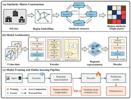
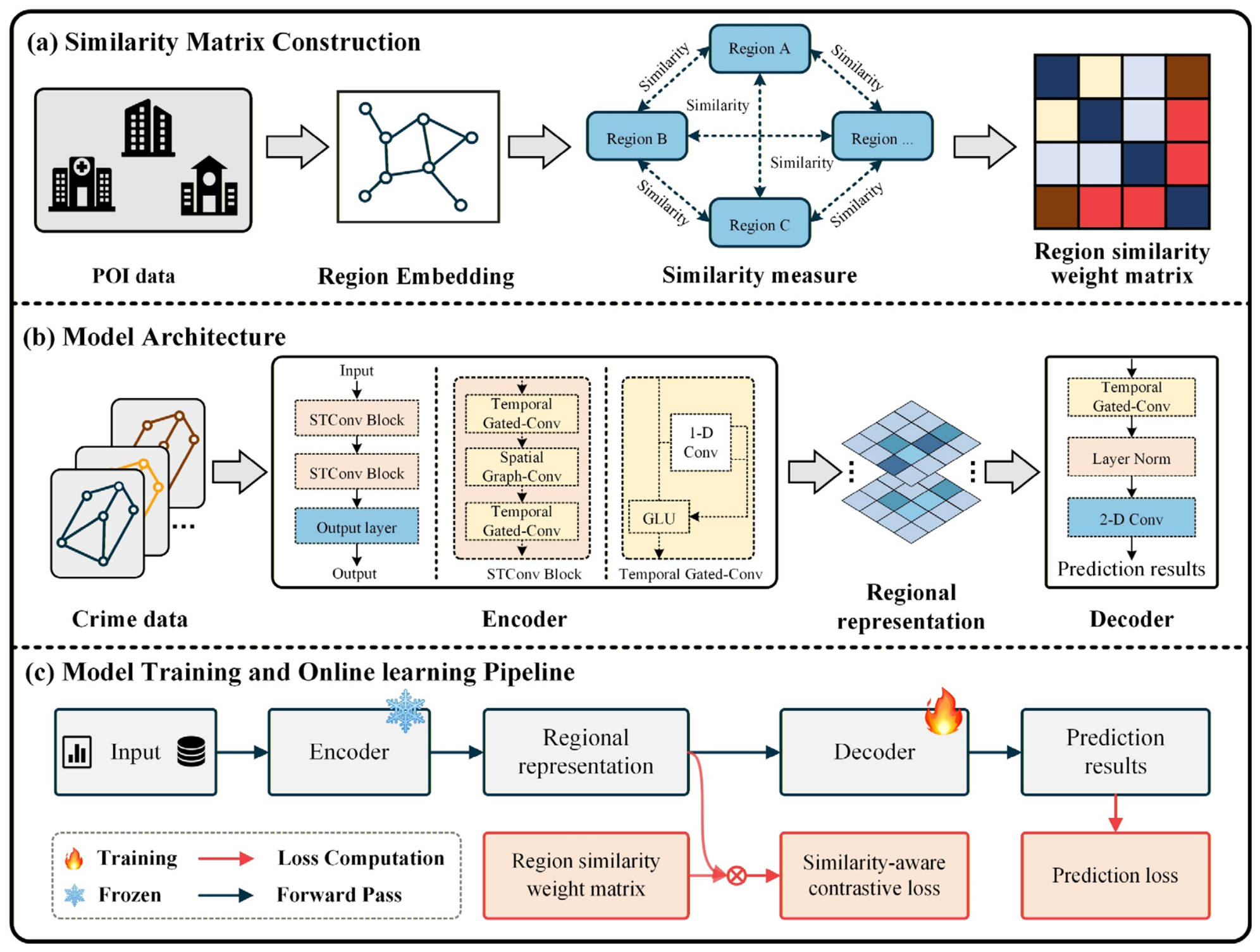
The region similarity weight matrix is designed to characterize the spatial semantic similarity among different urban regions. Considering that crime patterns across regions often exhibit similarities and periodicity, effectively quantifying inter-regional relationships is crucial for enabling the model to better capture underlying spatiotemporal dynamics. As shown in Figure 1a, we construct spatial semantic representations for each region based on POI distribution vectors. Specifically, we first assign a spatial index encoding to each region. We then employ cosine similarity [29] to precisely quantify the differences in spatial semantic distributions across regions, as represented by the counts of various POI types. During this process, no normalization is applied to the raw counts of POIs, thereby retaining the intact volumetric variance and heterogeneities across different urban grids. For region $R^i$ and $R^j$, the formula of cosine similarity is defined as

$$cosine\left(R^i,R^j\right)={\displaystyle \frac{{<R}^i·R^j>}{{\left|\right|R^i\left|\right|}_F{\left|\right|R^j\left|\right|}_F}}$$

(2)

where ${<R}^i·R^j>=\sum _L{R}_L^i·R_L^j$ and ${\left|\right|·\left|\right|}_F$ is the Frobenius norm. $L$ is the number of spatial regions. Finally, we obtain a region similarity weight matrix ${SimA\in \mathbb{R}}^{L\times L}$. $SimA$ is further utilized to guide the construction of positive and negative samples in contrastive learning.

Figure 1. The overall architecture of SSG-OL, which consists of the STGNN encoder, model architecture, model training, and online learning process.

Importantly, cosine similarity is not used to measure absolute POI density; rather, it evaluates the relative proportions of different urban functional features within each region. This approach has been widely validated in the literature for capturing similarity patterns between regions [30]. Based on this, we construct a region similarity weight matrix to inform the subsequent similarity-aware contrastive loss. This design aims to reduce the representational distance in the latent feature space. Specifically, it brings closer together regions that are not spatially adjacent but exhibit highly similar urban functional structures.

2.2.2. Model Architecture

The overall framework of SSG-OL consists of a spatiotemporal encoder and a prediction decoder. Specifically, as shown in Figure 1b, the historical crime data are first fed into a Spatiotemporal Graph Convolutional Network (STGCN) to learn latent region representations, which are then passed to a decoder to predict future crime counts.

The encoder is composed of two stacked spatiotemporal convolutional (ST-Conv) blocks. The output of the first ST-Conv block is directly used as the input to the second ST-Conv block. Each ST-Conv block integrates spatial graph convolution for modeling spatial correlations among regions and temporal gated convolution for capturing temporal patterns, enabling the model to effectively learn regional representations. A layer normalization layer is applied after each ST-Conv block to stabilize training and improve convergence.

After passing through the two ST-Conv blocks, the learned latent representation is forwarded to the decoder module. The decoder consists of a temporal gated convolution layer followed by a Layer Normalization layer and a 2D convolution layer. Specifically, the temporal gated convolution extracts high-level temporal features from the latent representations produced by the ST-Conv blocks. The Layer Normalization layer then regularizes these hidden representations. Finally, the 2D convolution layer maps the hidden features to the prediction space to generate future crime counts. The following sections provide a detailed description of the model’s training and prediction phase.

2.2.3. Model Training Phase

The overall training pipeline of the proposed model is illustrated in Figure 1c. Specifically, the historical crime data over the past $T$ days are represented as $X\in {\mathbb{R}}^{L\times T}$ as input. The input is then fed into the STGCN encoder to learn spatiotemporal region representations $Z\in {\mathbb{R}}^{L\times T}$.

$$Z=f_{encoder}\left(X\right)$$

(3)

During the region representation learning process, to enhance the model’s ability to capture both similarity and heterogeneity among regions, we incorporate a spatial similarity-aware contrastive learning method [30]. Traditional contrastive learning typically treats augmented views of the same sample as positive pairs and views from different samples as negative pairs. However, this strategy has clear limitations in crime spatiotemporal prediction, where inter-regional similarity is not binary but exhibits semantic relationships. This is due to the complex interplay of multiple spatial factors shaping the crime distribution. For example, two adjacent commercial areas may share highly similar POI distributions and should be treated as strong positive pairs, whereas the association between a commercial area and a remote residential area is relatively weak.

Therefore, the core idea of our method is to leverage prior inter-regional similarity to guide the region representations, such that semantically similar regions are pulled closer while dissimilar regions are pushed apart. Instead of using a fixed threshold, we determine the boundaries between positive and negative samples by ranking them based on relative region similarity.

Specifically, for a pair of regions $i$ and $j$, their corresponding representations are denoted as $Z_i\in {\mathbb{R}}^T$ and $Z_j\in {\mathbb{R}}^T$, respectively. When the region similarity weight matrix $SimA(i,j)$ is higher, the representations $Z_i$ and $Z_j$ are encouraged to be closer in the region representation space. Based on this intuition, for a city with $L$ regions, a similarity-aware contrastive loss ${\mathcal{L}}_{scl}$ is constructed to optimize the encoder:

$${\mathcal{L}}_{scl}={\displaystyle \frac{1}{L\left(L-1\right)}}{\displaystyle \sum _i^L}{\displaystyle \sum _k^L}I\left(k\ne i\right){\mathcal{L}}_{simCL}^{\left(i,k\right)}$$

(4)

$${\mathcal{L}}_{simCL}^{\left(i,k\right)}=-log{\displaystyle \frac{exp\left(cosine\left(Z_i,Z_k\right)/\mathrm{\tau }\right)}{{\displaystyle {\sum }_j^L}I\left(j\ne i,SimA\left(i,k\right)\ge SimA\left(i,j\right)\right)exp\left(cosine\left(Z_i,Z_j\right)/\mathrm{\tau }\right)}}$$

(5)

where $\tau$ is a temperature hyperparameter, and $I$ is an indicator variable that takes the value of 0 or 1 to distinguish positive and negative pairs. By minimizing ${\mathcal{L}}_{scl}$, the encoder is guided to learn more discriminative and robust region representations.

This approach differs from traditional contrastive learning methods of defining positive and negative samples. It implements a soft contrastive mechanism based on similarity ranking. For a given region $i$, the target region $k$ in the numerator is treated as a positive sample, while in the denominator, other regions whose similarity does not exceed that of $k$ are considered soft negative samples. This design encourages positive samples to be pulled closer while attenuating the influence of negative samples, thereby achieving the objective of “bringing similar regions closer and pushing dissimilar regions apart.”

Finally, the learned region representations $Z$ are then fed into the decoder to generate the final crime prediction results $Y\in {\mathbb{R}}^{L\times T}$.

$$Y=f_{decoder}\left(Z\right)$$

(6)

During the training process, the Mean Squared Error (MSE) loss is adopted as the prediction objective to minimize the model outputs $Y$ and true crime count $\widehat{Y}$, ensuring the prediction accuracy.

In summary, during the SSG-OL training process, the total optimization objective can be expressed as follows:

$${\mathcal{L}}_{total}={\mathcal{L}}_{MSE}\left(Y,\widehat{Y}\right)+\lambda ·{\mathcal{L}}_{scl}$$

(7)

Algorithm 1 presents the pseudocode illustrating the training phase of the SSG-OL, detailing each stage of the optimization and update process.

Algorithm 1: SSG-OL Training Phase
Input: Training set $\mathcal{X}={\left\{(x_i,y_i)\right\}}_{i=1}^N;$ Encoder $f_{encoder}\left(·\right);$ Decoder $f_{decoder}\left(·\right).$
Output: Encoder $f_{encoder}\left(·\right);$ Decoder $f_{decoder}\left(·\right).$
1:	Initialization: Encoder parameter ${\theta }_{encoder}\left(·\right),$ Decoder parameter ${\theta }_{decoder}\left(·\right).$
2:	For each training epoch do:
3:	For each batch $(x_i,y_i)$ do:
4:	Obtain latent features $z_i=f_{encoder}\left(x_i\right).$
5:	Compute contrastive loss ${\mathcal{L}}_{scl}$: ${\mathcal{L}}_{scl}={\displaystyle \frac{1}{L\left(L-1\right)}}{\displaystyle {\sum }_i^L}{\displaystyle {\sum }_k^L}I\left(k\ne i\right){\mathcal{L}}_{simCL}^{\left(i,k\right)}.$
6:	Generate prediction results $Y_i=f_{decoder}\left(z_i\right).$
7:	Compute MSE loss: $\mathcal{L}={\mathcal{L}}_{MSE}(Y_i,{\widehat{Y}}_i).$
8:	Compute total loss: ${\mathcal{L}}_{total}={\mathcal{L}}_{MSE}\left(Y,\widehat{Y}\right)+\lambda ·{\mathcal{L}}_{scl}.$
9:	Update Encoder and Decoder parameters: $Optimizer\left({\nabla }_{{\mathcal{L}}_{total}}\right)\to ({\theta }_{encoder},{\theta }_{decoder}).$
10:	End for
11:	End for
12:	Return: Trained Encoder $f_{encoder}\left(·\right)$ and Decoder $f_{decoder}\left(·\right).$

2.2.4. Online Learning Phase

Traditional crime spatiotemporal prediction models follow an offline training paradigm and assume that the crime spatial distribution is stationary. However, in real-world scenarios, crime patterns are influenced by various dynamic factors, resulting in non-stationary and dynamic distributions [31]. Traditional models often struggle to solve this problem.

To address this issue, we propose an iterative online learning strategy to improve the model’s generalization ability for short-term crime prediction. Considering that the encoder is responsible for extracting spatiotemporal features and already possesses strong generalization capabilities after pretraining on extensive historical data, frequent updates to the encoder can lead to overfitting on recent data and cause the model to forget long-term patterns. In contrast, the decoder is relatively lightweight, allowing it to be updated more rapidly and adapt the prediction mapping to limited new data efficiently, while also reducing computational costs. Therefore, we adopt a conditional fine-tuning mechanism for both the encoder and decoder as illustrated in Figure 1c.

Specifically, after the initial training phase, the parameters of encoder ${\theta }_{encoder}$ are frozen, while only the parameters of the decoder ${\theta }_{decoder}$ are updated. During the prediction process, the decoder is updated every $n$ steps by minimizing the prediction loss $MSE(Y,\widehat{Y})$, allowing the model to rapidly adapt to short-term fluctuations in crime patterns and enhance its generalization ability. In our experiments, $n$ was regarded as a hyperparameter and adjusted to optimize performance.

Algorithm 2 presents the pseudocode illustrating the online learning phase of the SSG-OL, detailing each stage of the optimization and update process.

Algorithm 2: SSG-OL Online Learning Phase
Input: Test set $\mathcal{X}={\left\{(x_i,y_i)\right\}}_{i=1}^N;$ Pre-trained Encoder $f_{encoder}\left(·\right);$ Pre-trained Decoder $f_{decoder}\left(·\right).$
Output: Decoder $f_{decoder}\left(·\right).$
1:	Initialization: Encoder parameter ${\theta }_{encoder}\left(·\right),$ Decoder parameter ${\theta }_{decoder}\left(·\right).$
2:	For each batch $(x_i,y_i)$ do:
3:	Freeze $f_{encoder}\left(·\right),$ unfreeze $f_{decoder}\left(·\right).$
4:	Obtain latent features $z_i=f_{encoder}\left(x_i\right).$
5:	Generate prediction results $Y_i=f_{decoder}\left(z_i\right).$
6:	Compute MSE loss: $\mathcal{L}={\mathcal{L}}_{MSE}(Y_i,{\widehat{Y}}_i)$ and update ${\theta }_{f_d}.$
7:	Unfreeze $f_{decoder},$ freeze $f_{encoder}.$
8:	Stop gradient flow to Encoder ${\nabla }_{{\theta }_{encoder}}\mathcal{L}=0.$
9:	Compute gradients for Decoder: ${\theta }_{decoder}={\nabla }_{{\theta }_{decoder}}\mathcal{L}.$
10:	End for
11:	Return: Decoder $f_{decoder}\left(·\right).$

3. Experiment

This section describes the designed comparative experiment to validate the proposed method, including datasets, evaluation metrics, baselines, and experimental configurations.

3.1. Datasets

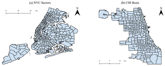
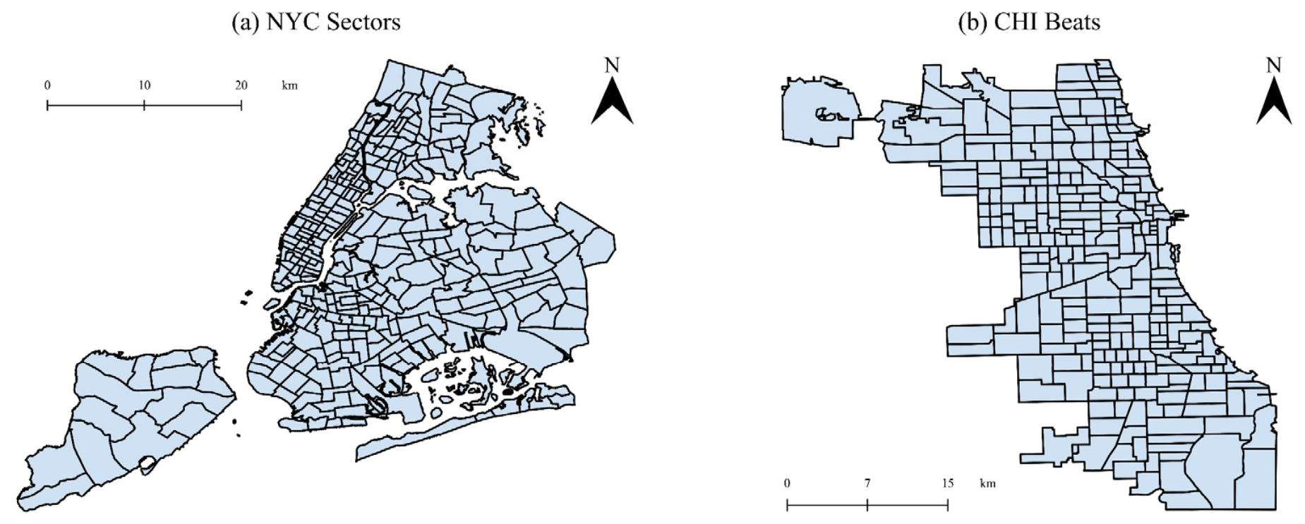
Our experiments are conducted on real-world crime datasets collected from two major U.S. cities: NYC and CHI. These cities provide comprehensive and long-term crime records, and many crime prediction models have been developed using data from these cities [31,32], ensuring the comparability of experimental results. Following prior studies [31,32], we adopt police administrative units (police beats and sectors) as the spatial granularity for crime prediction. Crime incidents are mapped to regions according to their corresponding geographic coordinates and aggregated on a daily basis. We remove records without valid geographic coordinates to ensure data quality. The spatial distribution of crime in each city is illustrated in Figure 2.

Figure 2. Spatial Distribution of NYC Sectors and CHI Beats.

For each city, we use two consecutive years of crime data, which are divided into training, validation, and test sets with a ratio of 7:1:2. We focus on property crimes and violent crimes, with detailed statistics reported in Table 1.

Table 1. Statistics of experimented urban crime datasets.

City	Time	Unit	Crime Types	Sub Crime Types	Cases
NYC	January 2022–December 2023	302 sectors	Property crime	Larceny and Theft, Motor Vehicle Theft, Burglary	396,961
			Violent crime	Assault, Robbery	200,960
CHI	January 2023–December 2024	277 beats	Property crime	Theft, Motor Vehicle Theft, Burglary	183,271
			Violent crime	Assault, Battery, Robbery	155,503

The POI data are collected from OpenStreetMap. Records without valid geographic coordinates are removed prior to analysis to ensure accurate spatial mapping. During the construction of the region similarity weight matrix, to mitigate data sparsity in spatiotemporal modeling, we follow prior crime modeling studies [33] and categorize POIs into three functional groups to mitigate inconsistencies in POI taxonomies across cities:

(1)

Basic services: This dimension characterizes the foundational administrative and lifestyle infrastructure of the urban space. It aggregates public governance sectors (e.g., police and fire station), essential social resources (e.g., university, hospital, pharmacy), sustenance venues (e.g., restaurant, cafe, bar), and cultural or leisure environments (e.g., park, stadium, museum).

(2)

Retail and wholesaling: This category maps the commercial vitality of the region, including consumption hubs (e.g., mall, supermarket, department store) and specialized commercial service entities (e.g., car dealership, mobile phone shop, furniture shop).

(3)

Public transportation: This category isolates the transit nodes and shared mobility options that dictate urban human mobility patterns, including fixed transit infrastructures (e.g., bus stop, tram stop) and transit services (e.g., car sharing, bicycle rental).

This categorization enables a more effective representation of spatial semantic characteristics across regions.

3.2. Evaluation Metrics

To evaluate the proposed model’s ability to predict future crime counts, we adopt MAE, RMSE, and mean hit rate as evaluation metrics. The definitions are as follows:

$$\mathrm{MAE}={\displaystyle \frac{1}{n}}{\sum }_{i=1}^n{|Y}_i-{\widehat{Y}}_i|$$

(8)

$$\mathrm{RMSE}=\sqrt{{\displaystyle \frac{1}{n}}{\sum }_{i=1}^n{\left(Y_i-{\widehat{Y}}_i\right)}^2}$$

(9)

$$\mathrm{Mean}\mathrm{hit}\mathrm{rate}={\displaystyle \frac{1}{T}}{\displaystyle \sum _{t=1}^T}{\displaystyle \frac{n_t}{N_t}}\times 100\%$$

(10)

where $n$ is the number of observations, ${\widehat{Y}}_i$ represents the actual values, and $Y_i$ represents the predicted values. Lower values of these metrics indicate better model performance. In mean hit rate, $n_t$ denotes the number of grids with actual crime counts among the top k% predicted at time $t$, $N_t$ denotes the total number of grids with actual crimes count at time $t$, and $T$ denotes the total number of time steps. In this study, we focus on the top 10% and 20% of regions in terms of crime hotspots.

3.3. Methods for Comparison

To validate the effectiveness of SSG-OL, we compare our model with the following baseline models:

(1)

Temporal graph convolutional network (TGCN) [34]: This model leverages GCN to encode spatial relationships and incorporates GRUs to capture long-term temporal dependencies in spatiotemporal sequences.

(2)

Spatiotemporal graph convolutional network (STGCN) [35]: This model utilizes gated temporal convolutions to learn temporal patterns and GCN to model spatial correlations.

(3)

Multivariate time series forecasting with graph neural network (MTGNN) [36]: This is a learnable graph network based on temporal convolution networks for temporal modeling and spatial correlation.

(4)

Adaptive graph convolutional recurrent network (AGCRN) [37]: This RNN architecture model learns adaptive graph structures and dynamic node embeddings.

(5)

Attention-based spatial-temporal graph convolutional networks (ASTGCN) [38]: This is an attention-based spatiotemporal GNN capable of capturing periodic temporal dependencies.

(6)

Spatiotemporal window attention model (ST-WA) [39]: This approach goes beyond standard attention mechanisms by incorporating specialized node features and time-dynamic parameters.

(7)

Generative pre-training of spatiotemporal graph neural network (GPT-ST) [40]: This is a generative pre-trained model based on spatiotemporal masked autoencoders and a hypergraph structure to capture multi-level spatial dependencies.

(8)

Opencity [41]: A hybrid architecture combining Transformers and GNNs, designed as a unified prediction framework with strong zero-shot generalization capability.

3.4. Experimental Configuration

This experiment was conducted in PyCharm using an RTX 4060 Ti GPU (NVIDIA, Santa Clara, CA, USA) and PyTorch 2.0.0. In our experiments, the input sequence length (the number of historical time steps) is set to 3, and the prediction horizon is also 3. All models are optimized by the Adam optimizer. The batch size is chosen from the set {8, 16, 24, 32} based on validation performance, and the number of epochs is set to 100. The learning rate is selected from the range [10⁻⁴, 10⁻¹] via grid search. For SSG-OL, we stack two STGCN layers for spatial and temporal context modeling. For the spatial convolutional and TCN layers, the kernel size is set as 3. The regularization weight $\lambda$ for the loss components is selected from the continuous interval (0.0, 1.0).

During the training stage, the model is first pretrained offline using the training dataset. During the testing stage, an online fine-tuning strategy is adopted, where incoming crime records are treated as a data stream. Once the accumulated data reach a predefined update interval, the model parameters are updated through incremental fine-tuning. Considering the temporal characteristics of crime patterns, we set the update cycle to 30 days. Accordingly, the model is fine-tuned and updated every 30 time steps of input data.

To ensure the reliability of the experimental results, each model is independently trained and evaluated five times. The final performance is reported as the mean value across these five runs. To further assess statistical significance, we compute a 95% confidence interval (CI) for each method based on the five repeated runs. In addition, we perform a paired t-test between the proposed method and the best-performing baseline, using the results obtained from the five independent runs of each model. The statistical significance is evaluated at a threshold of p < 0.05.

4. Results

This section analyzes the prediction results of the models from both macroscopic and microscopic perspectives. We first analyze the overall performance metrics from a macroscopic perspective. Table 2 presents the crime spatiotemporal prediction results of different models.

Table 2. Overall performance of urban crime prediction on four datasets.

Models	NYC Property Crime				NYC Violent Crime
	MAE	RMSE	10%	20%	MAE	RMSE	10%	20%
TGCN	1.172	1.574	0.225	0.366	0.943	1.400	0.210	0.362
STGCN	1.116	1.497	0.238	0.387	0.857	1.269	0.246	0.407
MTGNN	1.133	1.506	0.238	0.390	0.894	1.286	0.247	0.406
ASTGCN	1.162	1.546	0.233	0.369	0.890	1.369	0.205	0.348
AGCRN	1.164	1.553	0.229	0.368	0.926	1.399	0.215	0.356
ST-WA	1.364	1.812	0.126	0.228	0.836	1.458	0.134	0.255
GPT-ST	1.036	1.497	0.243	0.396	0.892	1.290	0.251	0.410
Opencity	1.019	1.473	0.246	0.390	0.925	1.396	0.205	0.348
SSG-OL	0.982 * (0.188)	1.359 * (0.186)	0.266 * (0.040)	0.421 * (0.044)	0.844 (0.019)	1.178 * (0.039)	0.290 * (0.011)	0.453 * (0.015)
Models	CHI property crime				CHI violent crime
	MAE	RMSE	10%	20%	MAE	RMSE	10%	20%
TGCN	0.269	0.587	0.133	0.240	0.414	0.613	0.120	0.230
STGCN	0.250	0.563	0.146	0.259	0.415	0.599	0.139	0.253
MTGNN	0.256	0.562	0.148	0.259	0.389	0.596	0.138	0.253
ASTGCN	0.269	0.587	0.133	0.241	0.417	0.615	0.120	0.228
AGCRN	0.271	0.587	0.129	0.237	0.413	0.614	0.119	0.227
ST-WA	0.287	0.604	0.100	0.196	0.445	0.622	0.097	0.196
GPT-ST	0.249	0.560	0.151	0.263	0.385	0.600	0.138	0.255
Opencity	0.272	0.592	0.132	0.240	0.413	0.617	0.120	0.228
SSG-OL	0.226 * (0.013)	0.503 * (0.042)	0.160 * (0.006)	0.271 * (0.003)	0.367 * (0.012)	0.579 * (0.009)	0.146 * (0.008)	0.264 * (0.009)

Note: Values in () indicate standard deviations. * denotes statistical significance at the 0.05 level (p < 0.05).

Table 2 presents the MAE, RMSE, and mean hit rates at the top 10% and 20% hotspot regions for property and violent crime prediction in NYC and CHI. Overall, SSG-OL achieves competitive performance across most evaluation metrics and experimental settings. Compared with conventional GNN models and pretrained approaches, SSG-OL consistently yields lower prediction errors, as evidenced by its reduced MAE and RMSE values. These results indicate the effectiveness of the proposed framework in capturing complex crime spatiotemporal patterns and improving prediction accuracy. For instance, SSG-OL decreases the MAE to 0.982 in the NYC property crime dataset, representing an improvement over Opencity and GPT-ST. This improvement suggests that the proposed model is effective in capturing complex and dynamic urban crime patterns.

From the perspective of practical law enforcement, the operational metrics (Top 10% and 20% mean hit rates) are of paramount importance for resource allocation. As demonstrated in Table 2, SSG-OL achieves the highest mean hit rates across the four datasets. In the NYC violent crime dataset, our model successfully locks down a 0.290 mean hit rate at the top 10% regions and a 0.453 mean hit rate at the top 20% regions. In Chicago datasets, SSG-OL similarly achieves improved prediction performance. This suggests that SSG-OL may provide useful support for crime hotspot identification and resource allocation under limited policing resources.

In addition, although the ST-WA model reports a marginally lower MAE than SSG-OL in the NYC violent crime dataset, this localized edge does not undermine the holistic superiority of our approach. Conversely, SSG-OL achieves stable prediction performance across different spatial units. Combined with its performance in the mean hit rates, SSG-OL indicates its effectiveness for complex urban crime prediction tasks.

5. Discussion

In this section, we further discuss the details of SSG-OL, including ablation analysis, convergence analysis, and other key parameters analyses.

5.1. Ablation Analysis

To further validate the effectiveness of the similarity-aware contrastive loss and online learning modules in learning robust representations, we conducted four sets of ablation experiments, where w/o Con denotes the removal of the contrastive loss module, Full Tune represents the full fine-tuning during the online learning phase, and w/o Online denotes the removal of the online learning mechanism. EWC (Elastic Weight Consolidation) [42] is a regularization-based online learning method, whereas ER (Experience Replay) [43] is a continual learning approach based on memory.

Table 3 details the ablation study and fine-tuning strategy analysis across four urban crime datasets. The baseline model, STGCN, functions as the architectural backbone. By evaluating the variants w/o Con and w/o Online, we observe a performance degradation across almost all evaluation metrics. Specifically, when the contrastive representation mechanism is absent, the model’s capacity to extract robust spatiotemporal features is compromised. Similarly, disabling the online adaptation streaming mechanism causes a noticeable drop in the mean hit rates at the top 10% and top 20% hotspot regions, particularly in datasets like NYC property. These results suggest that both contrastive representation learning and online streaming tuning are indispensable for capturing the nonlinear and dynamic urban crime distributions.

Table 3. Ablation analysis of urban crime prediction on four datasets.

Models	NYC Property Crime				NYC Violent Crime
	MAE	RMSE	10%	20%	MAE	RMSE	10%	20%
STGCN	1.116	1.497	0.238	0.387	0.857	1.269	0.246	0.407
w/o Con	1.111	1.497	0.238	0.388	0.919	1.323	0.246	0.406
w/o Online	1.089	1.483	0.240	0.390	0.895	1.296	0.245	0.406
Full Tune	1.027	1.478	0.248	0.402	0.917	1.321	0.246	0.406
EWC	1.030	1.483	0.248	0.401	0.801	1.080	0.255	0.418
ER	1.091	1.484	0.240	0.392	0.893	1.292	0.245	0.407
Our	0.982	1.359	0.266	0.421	0.844	1.178	0.290	0.453
Models	CHI property crime				CHI violent crime
	MAE	RMSE	10%	20%	MAE	RMSE	10%	20%
STGCN	0.250	0.563	0.146	0.259	0.415	0.599	0.139	0.253
w/o Con	0.260	0.567	0.148	0.256	0.378	0.597	0.137	0.252
w/o Online	0.254	0.571	0.149	0.260	0.387	0.601	0.137	0.252
Full Tune	0.251	0.563	0.152	0.264	0.401	0.608	0.135	0.251
EWC	0.251	0.558	0.151	0.262	0.391	0.602	0.139	0.255
ER	0.257	0.570	0.148	0.260	0.391	0.601	0.137	0.253
Our	0.226	0.503	0.160	0.271	0.367	0.579	0.146	0.264

Furthermore, we systematically compare our fine-tuning strategy with full model fine-tuning and other continual learning methods, including EWC and ER, which are based on either regularization or memory. While Full Tune optimizes all network parameters on new streaming batches without regularized constraints, it is more susceptible to catastrophic forgetting. Compared to the classic replay baseline ER, our proposed framework achieves the overall best performance in terms of error minimization and hotspot localized tracking across the majority of datasets. This numerical mismatch implies that while other online learning methods aggressively penalize changes to historically important weights to maintain a lower global average error, they may over-smooth the localized network responses, potentially reducing the model’s ability to adapt to emerging crime hotspots. Given that predictive policing prioritizes high-risk area interception, our model provides substantially higher real-world deployable value and hotspot capturing capabilities.

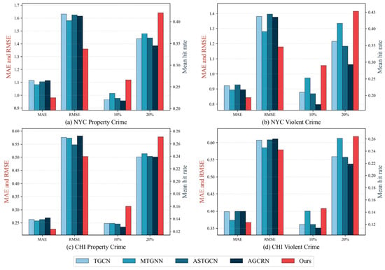
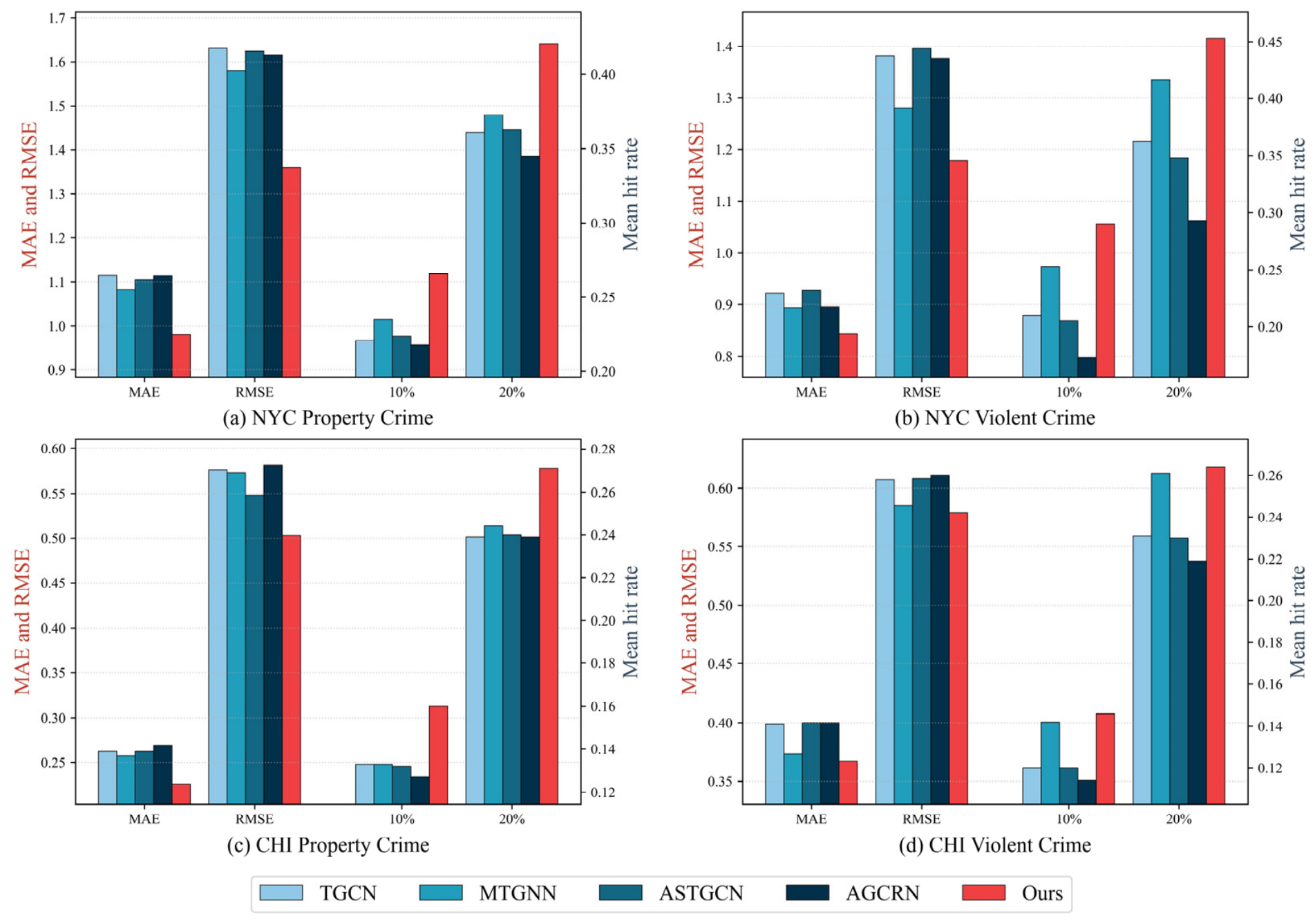
Figure 3 illustrates the performance of our framework across different spatiotemporal encoders on the four crime datasets. The findings show that our complete framework consistently outperforms all alternative encoder configurations. Concretely, other encoders suffer from higher regression errors and lower hotspot capturing capabilities. This superior performance of STGCN can be attributed to its unique architectural capacity to more effectively capture the intricate spatiotemporal heterogeneities inherent in urban crime distributions. Furthermore, the consistent trends observed across disparate crime categories and cities validate the generalizability of our design. Whether dealing with property or violent crimes, the STGCN as encoder enhanced by our framework consistently outperforms the baselines.

Figure 3. Ablation analysis of urban crime prediction on different encoders.

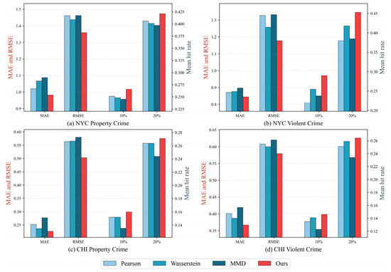
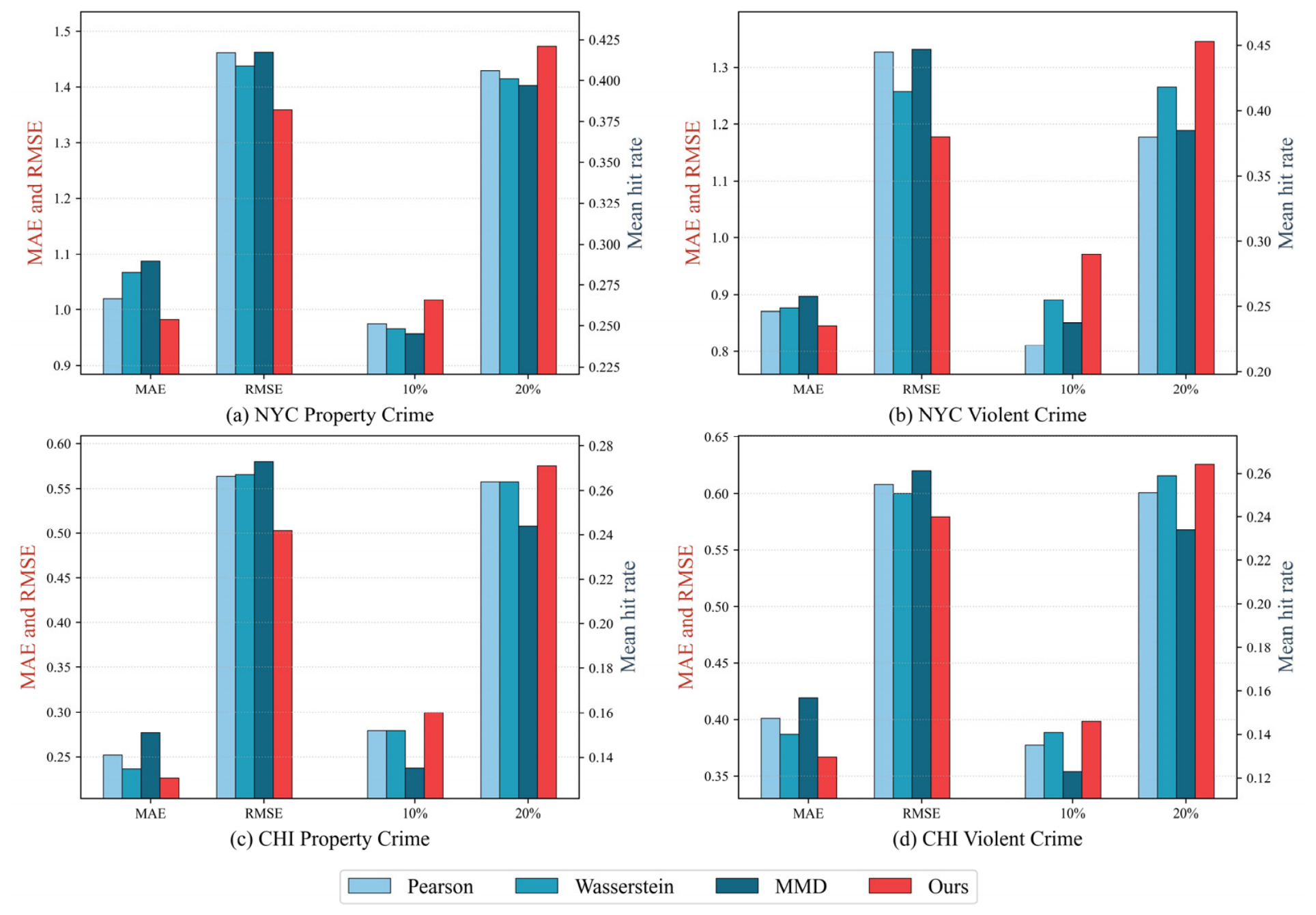
Figure 4 presents the comparison of crime prediction performance using different similarity measures. To evaluate the effect of spatial semantic alignment, we compare cosine similarity with three widely adopted alternatives, namely Pearson correlation, Wasserstein distance, and Maximum Mean Discrepancy (MMD). The results show that cosine similarity consistently achieves the best performance across all datasets. Compared with the other similarity measures, it produces lower MAE and RMSE values while simultaneously achieving the highest mean hit rates at both the top 10% and top 20% hotspot regions.

Figure 4. Ablation analysis of urban crime prediction on different similarity measures.

This result may be related to the fact that traditional metrics like Pearson correlation capture linear dependencies but are easily distorted by extreme data spikes or sparsity in crime-prone grids. Meanwhile, distribution alignment metrics such as Wasserstein and MMD distance focus heavily on global probability profiles, which often smooth out localized functional variations. In contrast, cosine similarity focuses on relative feature composition rather than magnitude differences. In the context of urban computing, this mathematical trait is highly beneficial as it focuses strictly on the proportional composition of urban functions. In summary, the results suggest that using cosine similarity to map spatial semantics allows the encoder to discover cross-regional crime correlations, making it an effective measure for modeling spatial semantic similarity.

5.2. Convergence Analysis

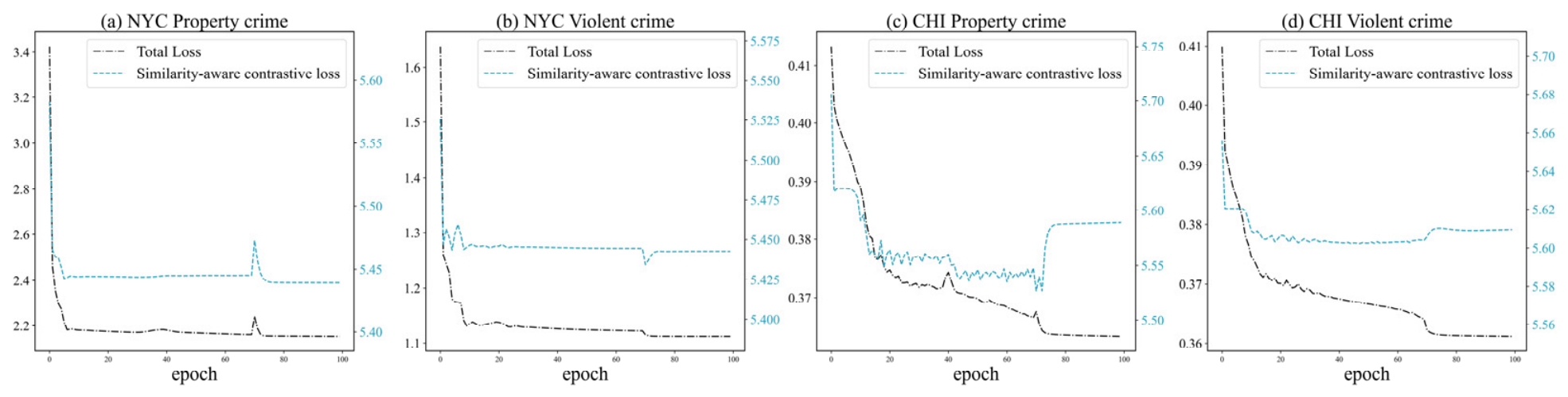
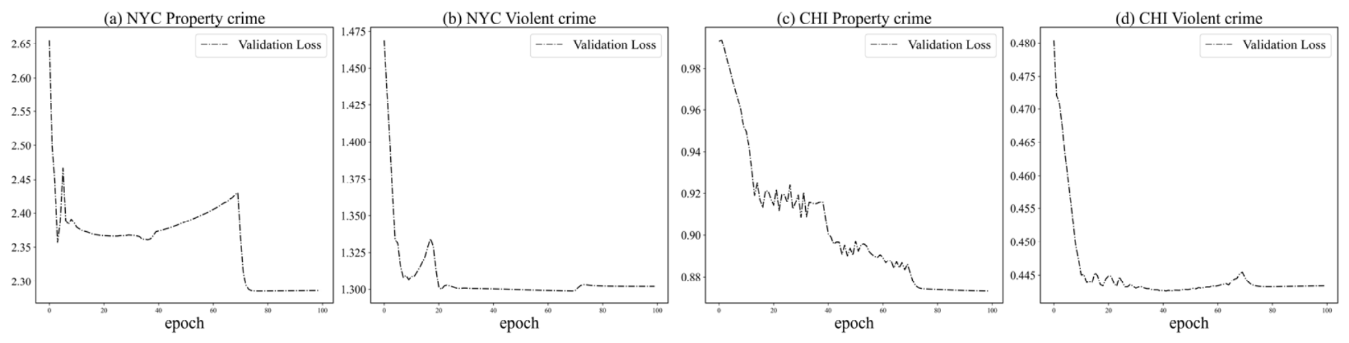
During the training process, the model optimizes its performance by minimizing both the prediction loss and the similarity-aware contrastive loss. To evaluate the convergence of SSG-OL, Figure 5 and Figure 6 illustrate the training dynamics of the model, including the evolution of the loss functions during training and the validation set performance.

Figure 5. Training loss and similarity-aware contrastive loss during model training process.

Figure 6. Validation loss during model training process.

Both the training and validation losses across all four tasks exhibit a rapid decline within the first 10 epochs. This initial sharp contraction suggests that our model can capture foundational spatiotemporal representations and effectively align regional semantics in the early phase of optimization.

Despite fluctuations in the optimization process, the loss functions exhibit overall stable convergence. For instance, in NYC property crime, minor fluctuations and spikes occur around epoch 10 and 70, followed by a dramatic drop to a lower steady state. Such step-down patterns may be associated with learning rate scheduling or optimization dynamics. As the learning rate scales down, the model may escape localized saddle points and refines its parameters into a finer optimization landscape. In addition, the similarity-aware contrastive loss stabilizes simultaneously with the Total loss, suggesting that our semantic matching mechanism establishes a useful constraint alongside the downstream prediction task.

Furthermore, the validation loss illustrated in Figure 6 provides our framework’s generalizability. In all four figures, after experiencing localized fluctuations, the validation loss smoothly converges to its global minimum and remains highly stable. This suggests relatively stable training behavior. The stable convergence at the tail end of both training and validation phases demonstrates stable training behavior across the evaluated datasets.

5.3. Parameter Sensitivity Analysis

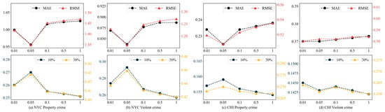
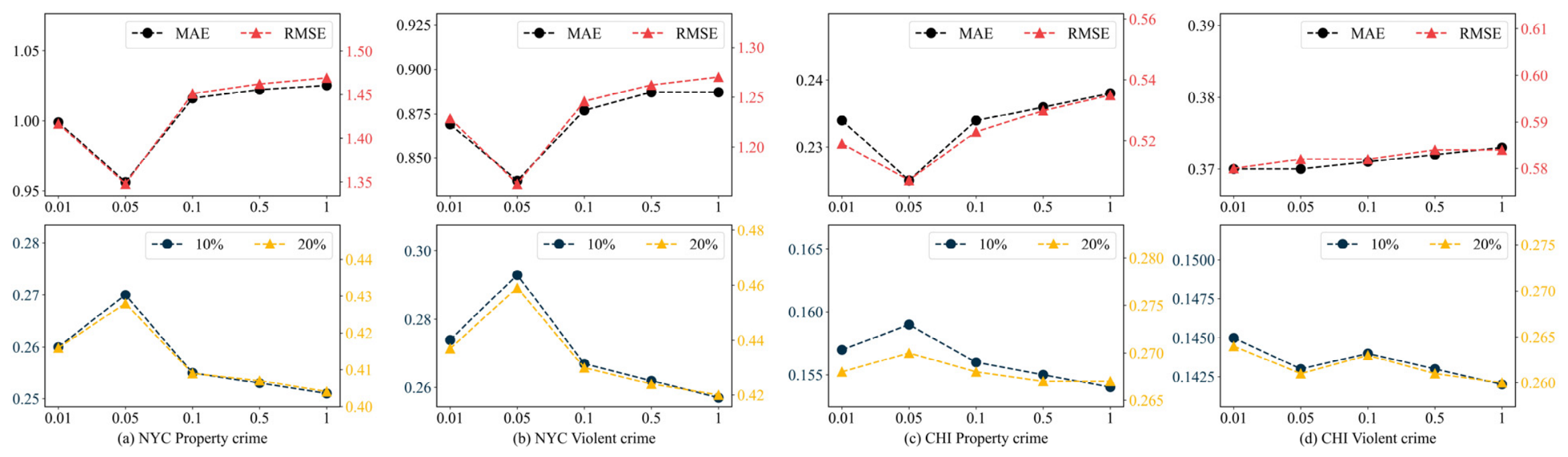
To evaluate the sensitivity of our model to key hyperparameters during training, we analyze the impact of the contrastive loss weight coefficient and the time steps of the online learning strategy in the SSG-OL module.

Figure 7 illustrates the prediction performance of SSG-OL under different weights of the similarity-aware contrastive loss. As illustrated in the parameter curves, when the parameter is set too small, the spatial semantic alignment constraint may remain under-optimized, resulting in suboptimal hotspot capturing performance. Conversely, aggressively increasing the parameter causes an increase in MAE and RMSE alongside a drop in the mean hit rates at the top 10% and top 20% hotspot regions. This degradation implies that an excessively large tradeoff value may over-regularize the model and degrade downstream prediction performance. Notably, across almost all datasets, the model achieves the best overall performance when the parameter is between 0.05 and 0.1.

Figure 7. Prediction performance of SSG-OL under different values of the tradeoff parameter $\lambda$.

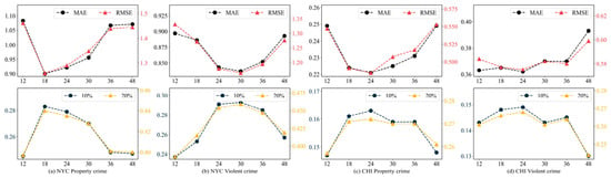
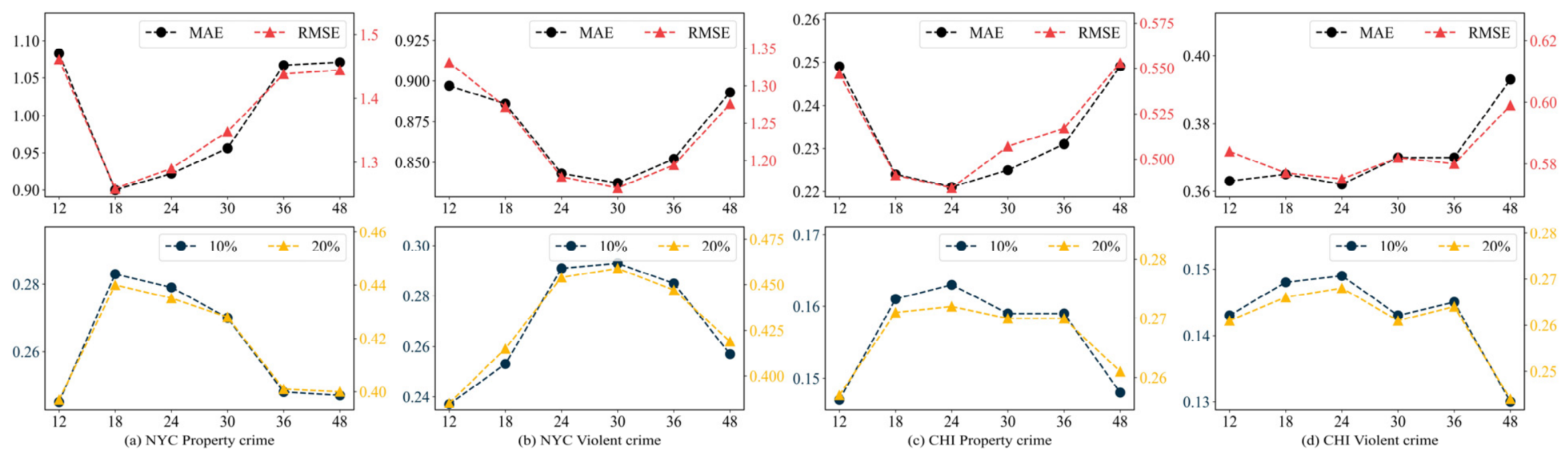
Furthermore, Figure 8 plots the sensitivity analysis of SSG-OL under different update time steps within the online learning strategy. The update time step indicates the temporal frequency at which the model adaptively updates its parameters based on incoming streaming batches. When the update interval is set too short (e.g., 12 h), the streaming windows may contain highly sparse crime signals, introducing noise and data fluctuations that hinder parameter convergence. On the other hand, extending the update window too long (e.g., 48 h) prevents the model from adaptively learning fine-grained temporal drifts and emerging hotspots.

Figure 8. Prediction performance of SSG-OL under different update time steps in the online learning strategy.

This analysis provides insights into the effect of update intervals on model performance. The optimal performance at an update interval of roughly 24 days may correspond to periodic urban activity patterns, such as monthly socio-economic cycles and human routine behavior shifts. In urban environments, micro crime fluctuations over periods of one to two weeks are often highly volatile. However, aggregating streaming data over a monthly update cycle allows more stable temporal patterns to emerge. This approach reduces the influence of noise while facilitating the capture of persistent behavioral changes and shifts in spatial distributions.

5.4. Computational Complexity and Efficiency Analysis

This section details the computational complexity and efficiency analysis of SSG-OL alongside three online learning strategies across the four datasets.

Table 4 presents the average execution time and GPU memory consumption required per single online adaptation step. The results show that SSG-OL achieves higher time efficiency than the compared methods. Across all datasets, SSG-OL achieves the fastest processing speed, reducing the execution time to approximately 6.2–6.6 milliseconds. In contrast, the baseline methods require substantially more processing time. The lower computational efficiency of EMC likely due to its graph exemplar selection and memory consolidation procedures. However, the training procedure of SSG-OL avoids some of these additional computational costs.

Table 4. Execution time and GPU memory consumption.

Models	NYC Property Crime		NYC Violent Crime
	Time (ms)	Memory (MB)	Time (ms)	Memory (MB)
EMC	15.861	327.854	15.597	327.854
ER	11.855	325.194	13.566	325.194
Full Tune	8.658	325.194	8.599	325.194
SSG-OL	6.611	325.194	6.220	325.194
Models	CHI property crime		CHI violent crime
	Time (ms)	Memory (MB)	Time (ms)	Memory (MB)
EMC	15.328	312.263	15.616	312.263
ER	11.961	309.724	12.415	309.724
Full Tune	8.396	309.724	8.340	309.724
SSG-OL	6.537	309.724	6.479	309.724

5.5. Spatial Visualization of Predicted Crime Risk

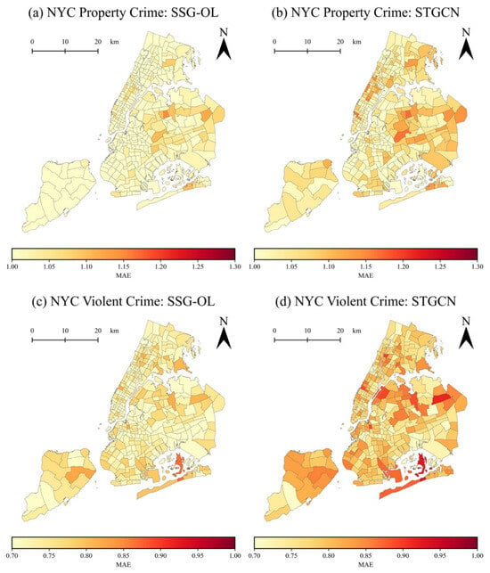
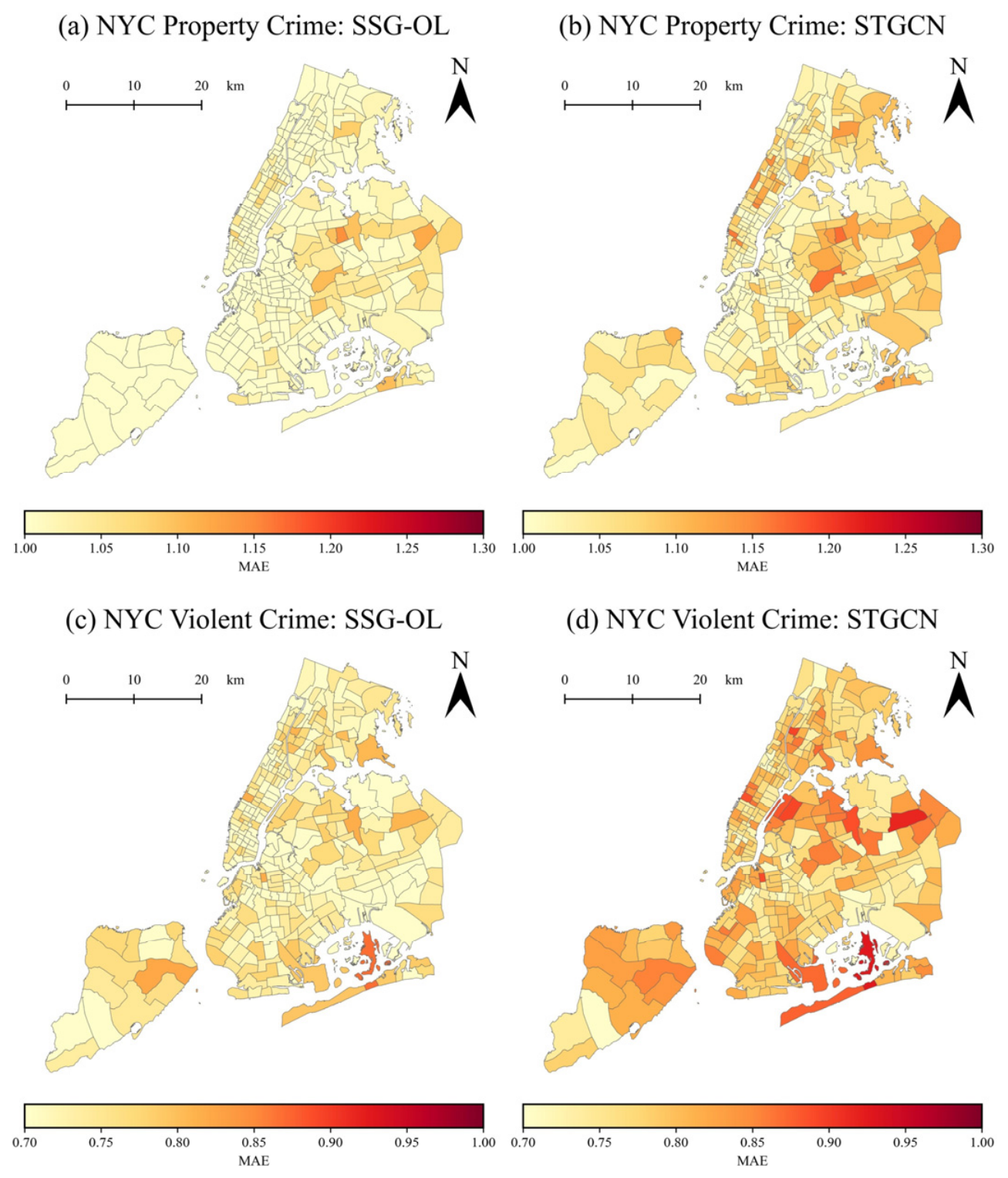
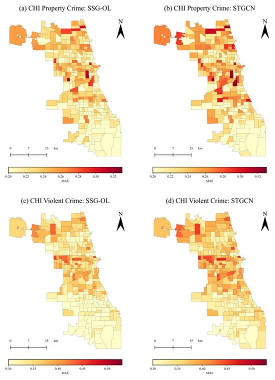
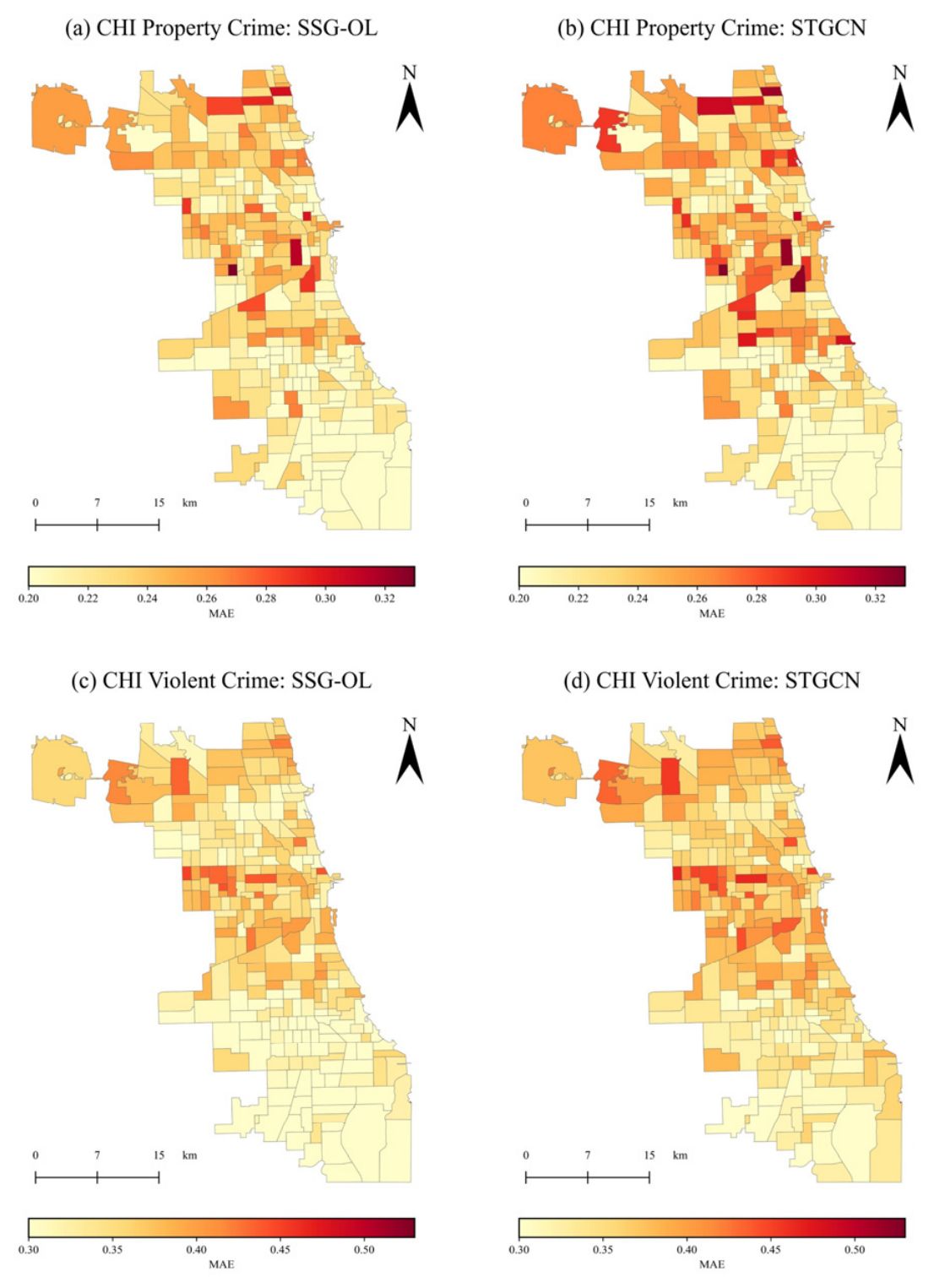
To further analyze the spatial distribution of prediction errors, we visualize the MAE values of SSG-OL. Specifically, we aggregate the MAE values over the test set onto a spatial visualization. To illustrate the effectiveness of our proposed SSG-OL, we chose the conventional STGCN model as the comparison baseline. Figure 9 and Figure 10 present the spatial distribution of MAE across the four datasets.

Figure 9. Spatial MAE Distribution of SSG-OL and STGCN for NYC property and violent crimes.

Figure 10. Spatial MAE Distribution of SSG-OL and STGCN for CHI property and violent crimes.

Figure 9 illustrates the spatial distribution of prediction errors for property and violent crimes in NYC using SSG-OL and STGCN. For property crimes, it is evident that SSG-OL achieves lower prediction errors across most areas compared with STGCN. For violent crimes, although prediction errors are generally low for both models, SSG-OL still exhibits lower errors in some regions. Similarly, Figure 10 shows the spatial comparison between the two models. The results indicate that SSG-OL not only achieves lower errors overall but also produces a more uniform error distribution. The number of high-error regions is reduced, while STGCN exhibits pronounced error concentrations, particularly along city edges and local hotspots. These observations suggest that SSG-OL may better capture spatial heterogeneity in urban crime patterns, improving predictive accuracy across diverse regions.

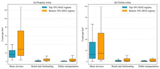
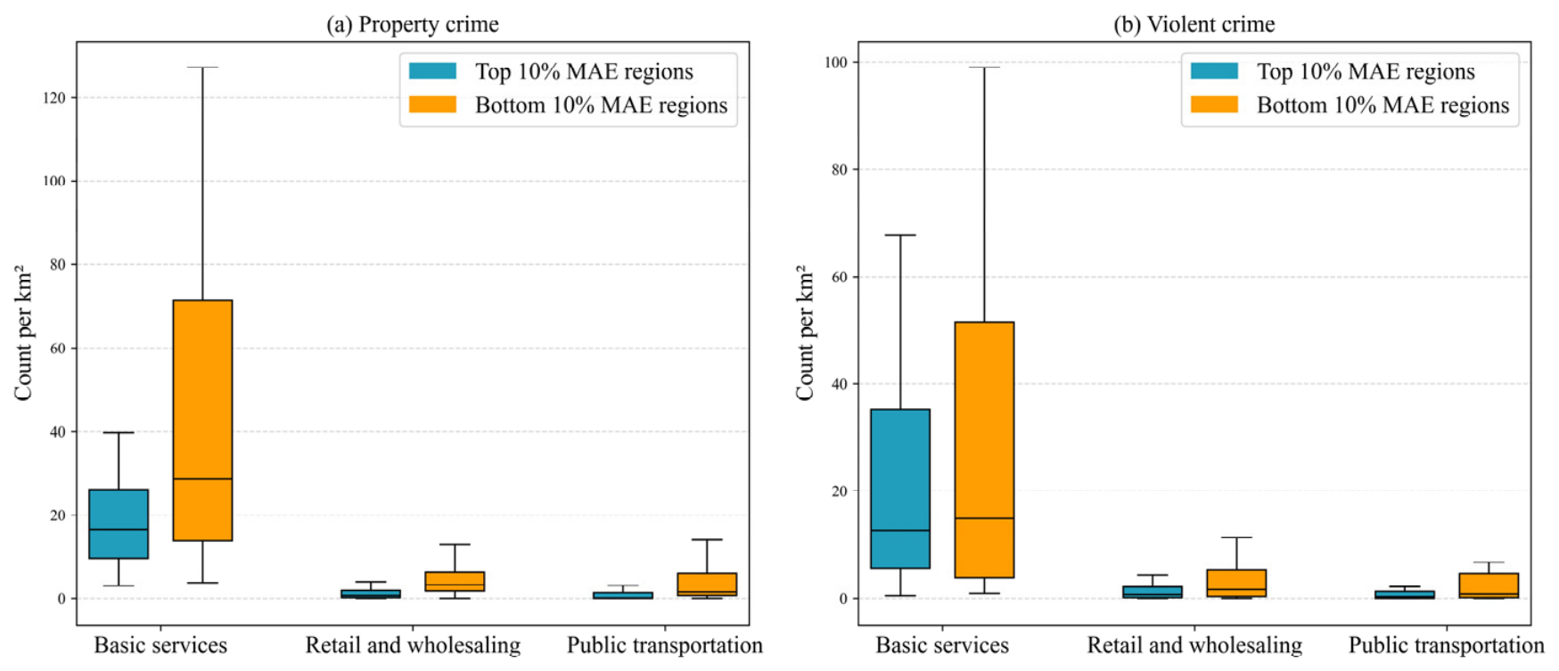
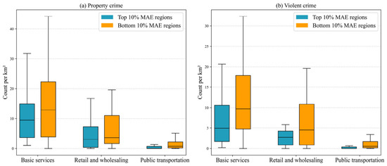
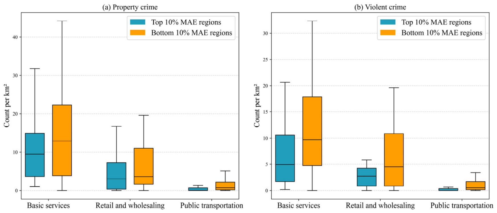
However, some regions exhibit relatively high prediction errors. To investigate the potential factors contributing to these errors, Figure 11 and Figure 12 compare the POI densities of the top 10% and bottom 10% MAE regions. The results indicate that areas with lower prediction errors tend to have higher POI density than those with higher errors. From the perspective of RAT, this observation suggests a potential association between POI density and prediction performance. These findings provide preliminary evidence that POI distributions may be associated with prediction performance. Therefore, it is necessary to enhance the model’s ability to perceive the heterogeneity among urban regions.

Figure 11. Comparison of POI density between the top and bottom MAE regions for property and violent crimes in NYC.

Figure 12. Comparison of POI density between the top and bottom MAE regions for property and violent crimes in NYC.

5.6. Cross-City Generalization Verification

To further evaluate the generalizability and practical scalability of the proposed framework, we conduct an additional cross-city generalization experiment on a crime dataset collected from a representative city, HN, located in the Yangtze River Delta region of China. HN is situated among the core cities of the delta, exhibits relatively high economic development, and possesses characteristics typical of medium sized cities, which allows us to evaluate the potential cross-city applicability of the model. This experiment serves as a complementary validation to the main evaluation on NYC and CHI, aiming to assess the model’s robustness under different socio-economic and geographical contexts.

The study period spans from January 2015 to December 2018. To mitigate the effects of data sparsity and ensure stable parameter mapping, the study area is partitioned into grids at a 3 km spatial resolution for crime spatiotemporal prediction [1]. The comprehensive evaluation results are summarized in Table 5.

Table 5. Overall performance of urban crime prediction on HN.

Models	HN Property Crime				HN Violent Crime
	MAE	RMSE	10%	20%	MAE	RMSE	10%	20%
TGCN	0.066	0.280	0.426	0.508	0.013	0.102	0.364	0.453
STGCN	0.067	0.262	0.430	0.509	0.015	0.102	0.374	0.475
MTGNN	0.051	0.263	0.432	0.508	0.014	0.101	0.311	0.396
ASTGCN	0.063	0.282	0.440	0.494	0.015	0.101	0.337	0.457
AGCRN	0.121	0.298	0.423	0.493	0.015	0.104	0.331	0.332
ST-WA	0.109	0.354	0.404	0.427	0.014	0.100	0.381	0.483
GPT-ST	0.073	0.278	0.464	0.551	0.014	0.102	0.365	0.457
Opencity	0.056	0.268	0.430	0.508	0.014	0.102	0.370	0.459
SSG-OL	0.054 (0.008)	0.246 * (0.015)	0.483 * (0.003)	0.560 * (0.001)	0.015 (0.005)	0.097 * (0.007)	0.402 * (0.046)	0.489 * (0.019)

Note: Values in () indicate standard deviations. * denotes statistical significance at the 0.05 level (p < 0.05).

Table 5 reports the comparative prediction performance on the HN dataset. As indicated by the metrics, SSG-OL shows lower prediction errors compared with other baselines. For property crime, although MTGNN yields a slightly lower MAE, SSG-OL achieves the lowest RMSE among the models. For violent crime, SSG-OL similarly secures the optimal error with a minimum RMSE. Furthermore, the mean hit rates at top 10% and 20% hotspot regions indicate that SSG-OL can accurately identify high-crime regions. In both property and violent crime categories, SSG-OL consistently outperforms advanced spatiotemporal prediction models. These results suggest that our approach may adapt to local geographic contexts and produce stable prediction performance.

6. Conclusions

In this paper, we proposed SSG-OL, a spatial semantic-guided spatiotemporal prediction framework with an online learning mechanism for crime spatiotemporal prediction. Extensive experiments on NYC and CHI crime datasets indicate that SSG-OL consistently achieves lower MAE and RMSE than state-of-the-art baselines in most cases. The results indicate that spatial semantic-guided contrastive learning contributes to modeling spatiotemporal dependencies and heterogeneity, while the online updating mechanism enhances the model’s adaptability to dynamic temporal patterns, which may enhance the model’s adaptability across different temporal patterns.

However, several limitations remain. First, the performance of SSG-OL is sensitive to the weighting of the contrastive loss, requiring careful parameter tuning. In future work, we will focus on developing more adaptive weighting strategies and exploring lightweight or self-adaptive semantic representations to further improve model generalization. Second, the construction of the spatial semantic similarity matrix remains relatively simplified. The current framework measures spatial semantic similarity using cosine similarity computed from POI category distributions. This representation may not fully capture the multifaceted nature of urban similarity. Factors such as population density, land use, and mobility flows may also contribute to functional relationships between regions. The absence of these factors in the similarity matrix could limit the completeness of the learned spatial semantics. Future work may explore the integration of multi-source urban data to develop more comprehensive representations of regional similarity. In addition, future work will extend the evaluation of the model to multiple additional cities, aiming to validate its robustness and adaptability to different urban environments.

References

- Li, Z.; Huang, C.; Xia, L.; Xu, Y.; Pei, J. Spatial-Temporal Hypergraph Self-Supervised Learning for Crime Prediction. In Proceedings of the 2022 IEEE 38th International Conference on Data Engineering (ICDE); IEEE: New York, NY, USA, 2022; pp. 2984–2996. [Google Scholar] [CrossRef] [Scilit]
- Lee, Y.; Bradford, B.; Posch, K. The Effectiveness of Big Data-Driven Predictive Policing: Systematic Review. Justice Eval. J. 2024, 7, 127–160. [Google Scholar] [CrossRef] [Scilit]
- Mohler, G.O.; Short, M.B.; Brantingham, P.J.; Schoenberg, F.P.; Tita, G.E. Self-Exciting Point Process Modeling of Crime. J. Am. Stat. Assoc. 2011, 106, 100–108. [Google Scholar] [CrossRef] [Scilit]
- Noor, T.H.; Almars, A.M.; Alwateer, M.; Almaliki, M.; Gad, I.; Atlam, E.-S. SARIMA: A Seasonal Autoregressive Integrated Moving Average Model for Crime Analysis in Saudi Arabia. Electronics 2022, 11, 3986. [Google Scholar] [CrossRef] [Scilit]
- McLafferty, S.; Williamson, D.; McGuire, P.G. Identifying Crime Hot Spots Using Kernel Smoothing. In Analyzing Crime Patterns: Frontiers of Practice; SAGE Publications, Inc.: Thousand Oaks, CA, USA, 2000; pp. 77–86. [Google Scholar] [CrossRef] [Scilit]
- Ramsahai, E.; Dookeram, N.; Ramsook, D.; Rameshwar, J.R.; Yearwood, A.B.; Bachoo, A.; Khan, K. Crime Prediction in Trinidad and Tobago Using Big Data Analytics. Int. J. Data Sci. Anal. 2023, 15, 421–432. [Google Scholar] [CrossRef] [Scilit]
- Alves, L.G.A.; Ribeiro, H.V.; Rodrigues, F.A. Crime Prediction through Urban Metrics and Statistical Learning. Phys. A Stat. Mech. Its Appl. 2018, 505, 435–443. [Google Scholar] [CrossRef] [Scilit]
- Yan, Z.; Chen, H.; Dong, X.; Zhou, K.; Xu, Z. Research on Prediction of Multi-Class Theft Crimes by an Optimized Decomposition and Fusion Method Based on XGBoost. Expert Syst. Appl. 2022, 207, 117943. [Google Scholar] [CrossRef] [Scilit]
- Hajela, G.; Chawla, M.; Rasool, A. A Clustering Based Hotspot Identification Approach for Crime Prediction. Procedia Comput. Sci. 2020, 167, 1462–1470. [Google Scholar] [CrossRef] [Scilit]
- Kang, H.-W.; Kang, H.-B. Prediction of Crime Occurrence from Multi-Modal Data Using Deep Learning. PLoS ONE 2017, 12, e0176244. [Google Scholar] [CrossRef] [Scilit] [PubMed]
- Dong, Q.; Li, Y.; Zheng, Z.; Wang, X.; Li, G. ST3DNetCrime: Improved ST-3DNet Model for Crime Prediction at Fine Spatial Temporal Scales. ISPRS Int. J. Geo-Inf. 2022, 11, 529. [Google Scholar] [CrossRef] [Scilit]
- Guo, Y. Multimodal Spatio-Temporal Fusion: A Generalizable GCN-LSTM with Attention Framework for Urban Application. Inf. Fusion 2026, 131, 104164. [Google Scholar] [CrossRef] [Scilit]
- Wang, S.; Zhang, Y.; Piao, X.; Lin, X.; Hu, Y.; Yin, B. MRAGNN: Refining Urban Spatio-Temporal Prediction of Crime Occurrence with Multi-Type Crime Correlation Learning. Expert Syst. Appl. 2025, 265, 125940. [Google Scholar] [CrossRef] [Scilit]
- Shan, M.; Ye, C.; Chen, P.; Peng, S. Ada-GCNLSTM: An Adaptive Urban Crime Spatiotemporal Prediction Model. J. Saf. Sci. Resil. 2025, 6, 226–236. [Google Scholar] [CrossRef] [Scilit]
- Gu, H.; Sui, J.; Chen, P. Graph Representation Learning for Street-Level Crime Prediction. ISPRS Int. J. Geo-Inf. 2024, 13, 229. [Google Scholar] [CrossRef] [Scilit]
- Ma, C.; Zhang, B.; Li, S.; Lu, Y. Urban Rail Transit Passenger Flow Prediction with ResCNN-GRU Based on Self-Attention Mechanism. Phys. A Stat. Mech. Its Appl. 2024, 638, 129619. [Google Scholar] [CrossRef] [Scilit]
- Lin, J.; Michailidis, G. A Multi-Task Encoder-Dual-Decoder Framework for Mixed Frequency Data Prediction. Int. J. Forecast. 2024, 40, 942–957. [Google Scholar] [CrossRef] [Scilit]
- Wei, C.; Li, W.; Zhang, Y.; Guan, J.; Zhou, S. MVST: A Multi-View Spatial-Temporal Model for Fine-Grained Crime Prediction. ACM Trans. Intell. Syst. Technol. 2025, 16, 1–22. [Google Scholar] [CrossRef] [Scilit]
- Liang, W.; Wang, Y.; Tao, H.; Cao, J. Towards Hour-Level Crime Prediction: A Neural Attentive Framework with Spatial–Temporal-Categorical Fusion. Neurocomputing 2022, 486, 286–297. [Google Scholar] [CrossRef] [Scilit]
- Jing, C.; Lv, X.; Wang, Y.; Qin, M.; Jin, S.; Wu, S.; Xu, G. A Deep Multi-Scale Neural Networks for Crime Hotspot Mapping Prediction. Comput. Environ. Urban Syst. 2024, 109, 102089. [Google Scholar] [CrossRef] [Scilit]
- Li, Z.; Xia, L.; Tang, J.; Xu, Y.; Shi, L.; Xia, L.; Yin, D.; Huang, C. UrbanGPT: Spatio-Temporal Large Language Models. In Proceedings of the 30th ACM SIGKDD Conference on Knowledge Discovery and Data Mining; Association for Computing Machinery: New York, NY, USA, 2024; pp. 5351–5362. [Google Scholar] [CrossRef] [Scilit]
- Cheng, H.; Gong, Z.; Wang, C. LLM-TFP: Integrating Large Language Models with Spatio-Temporal Features for Urban Traffic Flow Prediction. Appl. Soft Comput. 2025, 177, 113174. [Google Scholar] [CrossRef] [Scilit]
- Chen, Z.; Liu, D.; Xu, H.; Xu, Z.; Xu, L.; Zhou, J.; Du, W.; Chen, N. Risk Assessment of Typical Criminal Events in Urban Street View Images Based on Large Language Model and Deep Learning Method. Geo-Spat. Inf. Sci. 2026, 1–16. [Google Scholar] [CrossRef] [Scilit]
- De Nadai, M.; Xu, Y.; Letouzé, E.; González, M.C.; Lepri, B. Socio-Economic, Built Environment, and Mobility Conditions Associated with Crime: A Study of Multiple Cities. Sci. Rep. 2020, 10, 13871. [Google Scholar] [CrossRef] [Scilit] [PubMed]
- Qiu, M.; Wang, X.; Wu, Y.; Luo, A. The Forecast of the Number of Police Cases Based on Time Series and Convolutional Neural Network Model. Autom. Control Comput. Sci. 2022, 56, 230–238. [Google Scholar] [CrossRef] [Scilit]
- Du, Y.; Ding, N. A Systematic Review of Multi-Scale Spatio-Temporal Crime Prediction Methods. ISPRS Int. J. Geo-Inf. 2023, 12, 209. [Google Scholar] [CrossRef] [Scilit]
- Brantingham, P.; Brantingham, P. Criminality of Place: Crime Generators and Crime Attractors. Eur. J. Crim. Policy Res. 1995, 3, 5–26. [Google Scholar] [CrossRef] [Scilit]
- Kounadi, O.; Ristea, A.; Araujo, A.; Leitner, M. A Systematic Review on Spatial Crime Forecasting. Crime. Sci. 2020, 9, 7. [Google Scholar] [CrossRef] [Scilit] [PubMed]
- Zhao, X.; Fan, W.; Liu, H.; Tang, J. Multi-Type Urban Crime Prediction. Proc. AAAI Conf. Artif. Intell. 2022, 36, 4388–4396. [Google Scholar] [CrossRef] [Scilit]
- Hao, X.; Wan, H.; Guo, S.; Lin, Y. Balancing Imbalance: Data-Scarce Urban Flow Prediction via Spatio-Temporal Balanced Transfer Learning. In Proceedings of the Thirty-Fourth International Joint Conference on Artificial Intelligence; International Joint Conferences on Artificial Intelligence: Vienna, Austria, 2025; pp. 2865–2873. [Google Scholar] [CrossRef] [Scilit] [PubMed]
- Du, K.; Kang, Y.; Yang, X.; Shao, W. ST-HHOL: Spatio-Temporal Hierarchical Hypergraph Online Learning for Crime Prediction. In Proceedings of the Fourteenth International Conference on Learning Representations (ICLR); International Conference on Learning Representations (ICLR): Rio de Janeiro, Brazil, 2026. [Google Scholar]
- Ning, Y.; Liu, H.; Wang, H.; Zeng, Z.; Xiong, H. UUKG: Unified Urban Knowledge Graph Dataset for Urban Spatiotemporal Prediction. In Proceedings of the Advances in Neural Information Processing Systems; Neural Information Processing Systems Foundation, Inc. and Curran Associates, Inc.: Red Hook, NY, USA, 2023; Volume 36, pp. 62442–62456. [Google Scholar]
- Liu, L.; Gu, X.; Lan, M.; Zhou, H.; Chen, D.; Su, Z. Capturing the Spatial Arrangement of POIs in Crime Modeling. Comput. Environ. Urban Syst. 2025, 117, 102245. [Google Scholar] [CrossRef] [Scilit]
- Zhao, L.; Song, Y.; Zhang, C.; Liu, Y.; Wang, P.; Lin, T.; Deng, M.; Li, H. T-GCN: A Temporal Graph Convolutional Network for Traffic Prediction. IEEE Trans. Intell. Transp. Syst. 2020, 21, 3848–3858. [Google Scholar] [CrossRef] [Scilit]
- Yu, B.; Yin, H.; Zhu, Z. Spatio-Temporal Graph Convolutional Networks: A Deep Learning Framework for Traffic Forecasting. In Proceedings of the Twenty-Seventh International Joint Conference on Artificial Intelligence; AAAI Press: Washington, DC, USA, 2018; pp. 3634–3640. [Google Scholar]
- Wu, Z.; Pan, S.; Long, G.; Jiang, J.; Chang, X.; Zhang, C. Connecting the Dots: Multivariate Time Series Forecasting with Graph Neural Networks. In Proceedings of the 26th ACM SIGKDD International Conference on Knowledge Discovery & Data Mining; Association for Computing Machinery: New York, NY, USA, 2020; pp. 753–763. [Google Scholar]
- Bai, L.; Yao, L.; Li, C.; Wang, X.; Wang, C. Adaptive Graph Convolutional Recurrent Network for Traffic Forecasting. In Proceedings of the Advances in Neural Information Processing Systems; Curran Associates, Inc.: Red Hook, New York, USA, 2020; Volume 33, pp. 17804–17815. [Google Scholar]
- Guo, S.; Lin, Y.; Feng, N.; Song, C.; Wan, H. Attention Based Spatial-Temporal Graph Convolutional Networks for Traffic Flow Forecasting. Proc. AAAI Conf. Artif. Intell. 2019, 33, 922–929. [Google Scholar] [CrossRef] [Scilit]
- Cirstea, R.-G.; Yang, B.; Guo, C.; Kieu, T.; Pan, S. Towards Spatio-Temporal Aware Traffic Time Series Forecasting. In Proceedings of the 2022 IEEE 38th International Conference on Data Engineering (ICDE); IEEE: New York, NY, USA, 2022; pp. 2900–2913. [Google Scholar]
- Li, Z.; Xia, L.; Xu, Y.; Huang, C. GPT-ST: Generative Pre-Training of Spatio-Temporal Graph Neural Networks. In Proceedings of the Advances in Neural Information Processing Systems; Neural Information Processing Systems Foundation, Inc.: San Diego, CA, USA, 2023; Volume 36, pp. 70229–70246. [Google Scholar]
- Li, Z.; Xia, L.; Shi, L.; Xu, Y.; Yin, D.; Huang, C. Open spatio-temporal foundation models for traffic prediction. ACM Trans. Intell. Syst. Technol. 2025, accepted. [Google Scholar] [CrossRef] [Scilit]
- Kirkpatrick, J.; Pascanu, R.; Rabinowitz, N.; Veness, J.; Desjardins, G.; Rusu, A.A.; Milan, K.; Quan, J.; Ramalho, T.; Grabska-Barwinska, A.; et al. Overcoming Catastrophic Forgetting in Neural Networks. Proc. Natl. Acad. Sci. USA 2017, 114, 3521–3526. [Google Scholar] [CrossRef] [Scilit] [PubMed]
- Rolnick, D.; Ahuja, A.; Schwarz, J.; Lillicrap, T.; Wayne, G. Experience Replay for Continual Learning. In Proceedings of the Advances in Neural Information Processing Systems; Curran Associates, Inc.: Red Hook, NY, USA, 2019; Volume 32. [Google Scholar]
Disclaimer/Publisher’s Note: The statements, opinions and data contained in all publications are solely those of the individual author(s) and contributor(s) and not of MDPI and/or the editor(s). MDPI and/or the editor(s) disclaim responsibility for any injury to people or property resulting from any ideas, methods, instructions or products referred to in the content. |
© 2026 by the authors. Published by MDPI on behalf of the International Society for Photogrammetry and Remote Sensing. Licensee MDPI, Basel, Switzerland. This article is an open access article distributed under the terms and conditions of the Creative Commons Attribution (CC BY) license.