


Abstract
Day–night mobility differentiation provides important insights into the spatial organization of migrant activities, yet its spatial variation and underlying drivers remain insufficiently understood in Asian metropolitan areas. Using kernel density estimation (KDE), spatial autoregressive models, and multiscale geographically weighted regression (MGWR), the study examines how the built environment, socioeconomic context, economic attractiveness, and accessibility factors shape variations in migrant mobility across space among Chinese migrants in Seoul, South Korea. The results reveal pronounced spatial clustering, with higher levels of mobility differentiation concentrated in central and southeastern Seoul, whereas lower levels are observed in migrant-concentrated districts such as Guro-gu and Geumcheon-gu. Migrant stock is identified as the most influential and spatially consistent determinant, exhibiting a significant negative association across most areas. Land-use mix also negatively affects mobility differentiation, while office facilities, industrial facilities, and subway accessibility exert positive effects. Model comparison demonstrates that MGWR substantially outperforms ordinary least squares (OLS) and geographically weighted regression (GWR), achieving the highest explanatory power (R2 = 0.758; adjusted R2 = 0.705) and the lowest corrected Akaike information criterion (AICc) (763.656). Furthermore, MGWR uncovers considerable spatial heterogeneity in the effects of employment facilities, apartment concentration, and service-oriented facilities. These findings suggest that migrant day–night mobility differentiation is shaped by both citywide contextual factors and localized neighborhood characteristics, highlighting the importance of accounting for spatially varying relationships when examining migrant mobility patterns in metropolitan areas.
1. Introduction
Cities are increasingly understood as dynamic spatiotemporal systems shaped by the continuous movement of people, activities, and resources rather than as static physical entities [1,2,3,4]. As urbanization intensifies and daily activities become more spatially dispersed, human mobility has emerged as a fundamental mechanism through which urban spaces are produced, organized, and transformed [5,6]. Mobility influences how populations access employment, public services, social networks, and economic opportunities, while simultaneously reflecting broader patterns of inequality and socio-spatial differentiation [6,7,8,9]. Consequently, understanding mobility dynamics has become central to explaining how contemporary cities function and evolve [10,11,12,13].
Recent advances in mobile communication technologies and location-based data have significantly enhanced the ability to observe population dynamics at fine spatial and temporal scales [9,14,15,16]. These developments have revealed that urban spatial structures are not solely determined by physical land-use configurations but are also shaped by the temporal organization of everyday activities [17,18]. Mobility patterns vary considerably throughout the day because movements occurring during different periods are associated with distinct activity purposes, functional spaces, and social interactions [19,20,21]. Daytime mobility is typically linked to employment, education, and service-related activities, whereas nighttime mobility is more closely associated with residential routines, leisure, and social engagement [22,23]. Examining day–night mobility differentiation therefore provides a valuable perspective for understanding the temporal rhythms of urban life and the redistribution of population presence across urban space [16,24]. In this study, mobility refers to temporal changes in the spatial distribution of population presence derived from hourly population data rather than individual trajectories or origin–destination flows. Correspondingly, population redistribution describes shifts in population presence between daytime and nighttime periods, whereas mobility differentiation captures the spatial and temporal variations underlying such redistribution processes [1,25].
The importance of everyday mobility becomes particularly evident in the context of international migration [26,27]. Under globalization, migration has become a major driver of urban transformation, reshaping demographic structures, labor markets, housing systems, and local economies [26,28]. Increasingly, migration is understood not as a one-time residential relocation but as an ongoing process through which migrants interact with urban environments through daily activities, social relations, and economic participation [27,29]. Because migrants frequently encounter institutional, economic, and social constraints when accessing employment, housing, and public resources, their interactions with cities are often reflected in recurring mobility patterns connecting residential, workplace, and social spaces [27,29,30]. Examining migrant mobility therefore provides valuable insights into socio-spatial adaptation processes and the ways migrants engage with urban opportunities and constraints [27,31]. Importantly, this study does not directly measure migrant integration in its social, cultural, economic, or institutional dimensions; rather, it examines mobility patterns as indicators of migrants’ spatial interactions with the urban environment.
Despite growing scholarly interest in migration and urban mobility, existing research remains subject to several limitations. First, migrant studies have predominantly focused on residential settlement patterns [32], ethnic segregation [33], and socioeconomic outcomes [34] while paying comparatively limited attention to the dynamic mobility processes through which migrants experience cities in their everyday lives. Second, mobility studies have largely concentrated on aggregate movement patterns [12,35], commuting flows [36], tourism activities [37], or mobility responses to specific events [38], leaving routine day–night mobility dynamics insufficiently explored. Third, although built-environment characteristics, socioeconomic conditions, economic opportunities, and accessibility have been identified as important determinants of mobility [13,39,40], these influences are unlikely to be spatially uniform. Urban opportunities and constraints vary substantially across neighborhoods, generating localized mobility responses that conventional global models may fail to capture [16,40]. Finally, much of the existing theoretical and empirical evidence originates from European and North American contexts, leaving rapidly diversifying East Asian destination cities comparatively underexamined [29]. As a result, limited evidence exists regarding how urban contextual factors shape migrants’ day–night mobility patterns and how these relationships vary spatially within cities.
These gaps are particularly relevant in East Asia. Cities such as Seoul, Tokyo, and Singapore have experienced substantial growth in migrant populations as a result of globalization, labor-market restructuring, and demographic change [29,41,42]. Among migrant groups in Seoul, Chinese migrants constitute the largest foreign population and play a significant role in both ethnic and mainstream urban economies [43]. This population includes ethnic Koreans from China as well as other Chinese nationals [43,44]. For conceptual clarity, this study defines Chinese migrants as all individuals holding Chinese nationality regardless of ethnic background. Although analyzing all foreign residents could provide a broader perspective, substantial heterogeneity across migrant groups in terms of migration motives, and socioeconomic characteristics may obscure group-specific mobility mechanisms [45]. Focusing on Chinese migrants therefore enables a theoretically coherent and empirically robust examination of migrant mobility within a clearly defined population [46,47].
Against this background, this study investigates day–night mobility differentiation among Chinese migrants in Seoul using large-scale hourly population data and MGWR. Specifically, it pursues two objectives. First, it identifies the temporal rhythms and spatial redistribution patterns of Chinese migrants between daytime and nighttime periods. Second, it examines the spatially varying influences of built-environment, socioeconomic, economic, and accessibility factors on day–night mobility differentiation. Accordingly, the study addresses two research questions: (1) What spatial and temporal characteristics define day–night mobility differentiation among Chinese migrants in Seoul? and (2) How do urban contextual factors shape these patterns across neighborhoods? By integrating a day–night perspective with spatially explicit modeling, this study contributes to the literature in three ways. First, it advances research on migrant mobility beyond static residential perspectives toward a dynamic activity-based framework. Second, it reveals the spatial heterogeneity of factors influencing migrant mobility through the application of MGWR. Third, it provides empirical evidence from an underexamined East Asian context, contributing to a broader understanding of migration–mobility relationships in increasingly multicultural cities.
2. Materials and Methods
This study comprised three interrelated modules (Figure 1). (1) Constructing and pre-processing data: Multi-source mobility data and urban contextual information were integrated through standardized cleaning, normalization, and spatial alignment procedures to ensure temporal consistency and spatial comparability. (2) Analyzing spatial patterns: KDE, global spatial autocorrelation, and local indicators of spatial association (LISA) were employed to identify mobility hotspots, evaluate clustering tendencies, and detect localized spatial heterogeneity. (3) Modeling urban mechanisms: A MGWR framework was used to examine the spatially varying relationships between mobility patterns and urban factors, including the built environment, socioeconomic conditions, economic attractiveness, and accessibility.
Figure 1.
Analytical framework of the study. The workflow consists of three sequential stages: step 1 (red), step 2 (purple), and step 3 (blue).
2.1. Study Area and Data Description
2.1.1. Study Area
Seoul, the capital of South Korea, is the nation’s foremost economic, cultural, and technological center and a major metropolitan hub in Northeast Asia. The city covers approximately 605.96 km2 and is administratively divided into 25 districts (Gu) and 426 administrative neighborhoods (dong) (Figure 2). Within Seoul’s administrative system, the dong constitutes the smallest official spatial unit for urban management and statistical reporting. The administrative dong offers a fine spatial resolution for capturing intra-urban heterogeneity and identifying localized patterns of day–night mobility and their associated determinants. Therefore, the entire Seoul metropolitan area was selected as the study region, with the administrative dong adopted as the basic unit of analysis throughout this study.
Figure 2.
Administrative zoning map of Seoul. (a) South Korea. (b) Gu-level administrative divisions in Seoul. (c) Dong-level administrative divisions in Seoul. The gray-shaded areas in panel (c) represent the dong-level administrative divisions included in this study. The map was created using QGIS 3.34.1 and administrative boundary data obtained from the Seoul Open Data Plaza (SODP).
2.1.2. Data Sources and Preprocessing
(1) Population Mobility Data
Population mobility data were obtained from the Seoul Living Population Dataset provided by the SODP. The dataset integrates administrative population records with anonymized mobile communication signaling data supplied by KT Corporation and is designed to represent the de facto population physically present in Seoul at a given time [48,49]. Unlike conventional resident population statistics, the dataset captures both residents and non-residents regardless of their registered place of residence, thereby providing a more realistic representation of urban population distribution and activity intensity [50].
This study focused on Chinese migrants within Seoul’s long-term foreign resident population, defined as individuals residing in South Korea for more than 90 days and maintaining officially registered residential addresses. To capture routine mobility behavior, 51 valid weekdays between 1 January and 27 March 2026 were selected for analysis. Previous studies based on mobile phone signaling data have demonstrated that human mobility exhibits strong daily and weekly regularities, with weekday activities characterized by relatively stable spatiotemporal rhythms [16,48,49,51]. Consequently, recurring weekday observations provide a reliable basis for identifying routine activity structures and long-term behavioral tendencies. The selected observation period therefore provides sufficient temporal coverage to represent regular mobility patterns while reducing the influence of short-term anomalies and non-routine travel activities.
To identify day–night mobility differentiation, specific temporal windows were extracted from the dataset. Daytime activity spaces were represented by weekday working hours (09:00–18:00) [19,52], while nighttime residential locations were identified using the period from 02:00 to 04:00, which is widely recognized as the most stable interval of residential presence [53]. The morning commuting period (05:00–08:00) and evening transition period (17:00–01:00) were excluded because intensive movement during these periods may introduce spatial uncertainty and obscure the distinction between residential and activity spaces [19,52].
(2) Built Environment and Accessibility Data
Built environment data were obtained from the V-World National Spatial Information Open Platform, operated by the Ministry of Land, Infrastructure and Transport of South Korea. Accessibility data, including subway stations and road networks, were retrieved from the SODP. As of 14 May 2025, the dataset contained 301 subway stations and a road network with a total length of approximately 9600 km. To ensure spatial consistency, all spatial datasets were projected into the KGD2002 Central Belt 2010 coordinate system. Accessibility indicators were calculated using the Network Analyst extension in QGIS (version 3.34.1; Open Source Geospatial Foundation, Beaverton, OR, USA).
2.2. Variable Selection and Measurement
2.2.1. Dependent Variables
To capture day–night mobility differentiation among Chinese migrants, this study employed an absolute measure rather than ratio-based indicators. Specifically, the difference between daytime and nighttime populations was adopted, as it preserves the actual magnitude of population change and avoids the statistical instability associated with small denominators, particularly in low-population areas. Moreover, absolute measures are readily applicable to population exposure assessment analyses, thereby offering a more direct representation of mobility dynamics. The dependent variable was designed to reflect both the scale and temporal redistribution of migrant populations between day and night, and is calculated as follows [23]:
where denotes the net population difference in spatial unit , represents the daytime migrant population, and denotes the nighttime migrant population.
This indicator captures the intensity and direction of day–night mobility differentiation. A positive value of indicates a relative concentration of Chinese migrants during the daytime, whereas a negative value suggests a higher concentration at night. The magnitude of reflects the extent of temporal population redistribution, with larger absolute values indicating stronger differentiation between daytime and nighttime population distributions.
2.2.2. Explanatory Variables
Based on previous studies on urban mobility and immigrant spatial behavior, explanatory variables were classified into four analytical dimensions: built environment, socioeconomic context, economic attractiveness, and accessibility (Table 1).
Table 1.
Definition and measurement of the explanatory variables.
(1) Built Environment
Built environment characteristics have long been recognized as important determinants of residential location choice and daily mobility behavior [19,52]. The spatial distribution of land uses and development intensity shapes access to employment, services, and residential opportunities, thereby influencing where immigrants reside and conduct their daily activities [29,54,55,56]. Since immigrant settlement decisions are often path-dependent and constrained by information availability and adaptation costs, the built environment provides a critical spatial context that contributes to differentiated mobility patterns [29].
Three indicators were selected to characterize the built environment. First, Land-Use Mix measures functional diversity within each spatial unit using the Shannon entropy index based on the proportion of nine land-use categories. Areas with greater land-use diversity tend to integrate employment, commercial, and service functions, which may reduce travel distances and improve spatial efficiency, thereby influencing the organization of daily mobility [55,56]. Second, Floor Area Ratio represents the intensity of urban development and spatial capacity. Areas with higher development intensity generally serve as urban activity centers, attracting daytime populations and influencing the redistribution of nighttime populations. Third, Apartment Ratio reflects residential housing structure. In the Korean housing system, high-rise apartments are commonly associated with relatively higher housing prices and middle-class residential environments [29]. This creates a selective residential mechanism for immigrants and shapes nighttime residential concentration patterns.
(2) Socioeconomic Context
Socioeconomic context influences migrant settlement behavior by shaping residential affordability, social integration, and access to community resources [29]. Ethnic enclave research suggest that migrants tend to concentrate in neighborhoods where social networks, cultural familiarity, and support systems reduce settlement risks and adaptation costs [29]. At the same time, local living conditions affect residential stability and long-term neighborhood attachment.
Three indicators were therefore included. First, Migrant Stock represents the size of the Chinese population within each spatial unit [29]. This indicator reflects ethnic clustering and social network support. Higher immigrant concentration reduces information and adaptation costs, strengthens intra-community interaction, and increases nighttime stay probability. Second, Housing Price captures residential affordability [29,57]. This is calculated as the area-weighted average transaction price and logarithmically transformed to reduce skewness [29]. Variations in housing costs influence residential location choice and contribute to spatial separation between daytime workplaces and nighttime residences. Third, Facility Diversity measures the availability of services including healthcare, education, welfare, culture, and recreation [19,52]. Greater service diversity enhances neighborhood attractiveness and living convenience, indirectly shaping settlement stability and nighttime activity patterns.
(3) Economic Attractiveness
Employment opportunities constitute a fundamental driver of migrant residential location and mobility behavior [19,52]. The spatial distribution of employment influences commuting patterns and residential choices by determining the accessibility of workplaces for different labor groups [29]. Since migrants often exhibit heterogeneous labor-market characteristics, variations in local industrial structure can generate distinct patterns of daytime concentration and nighttime redistribution [29,58].
To capture local economic attractiveness, three employment-related indicators were selected. First, Office-Based Facility Density, measured by the proportion of office floor area, represents the concentration of advanced business functions and white-collar employment opportunities, which predominantly attract highly skilled immigrants during daytime periods. Second, Service-Oriented Facility Density represents the concentration of retail, catering, accommodation, and entertainment sectors. These industries generally have lower entry barriers and strong labor demand, providing critical employment opportunities for newly arrived migrants and contributing significantly to nighttime economic activities. Third, Industrial-Based Facility Density represents manufacturing and logistics activities associated with labor-intensive occupations. Such sectors tend to attract lower-skilled immigrants and generate work-oriented daytime commuting patterns.
(4) Accessibility
Accessibility is a key determinant of residential choice and spatial behavior because it influences commuting costs, employment access, and the spatial extent of daily activity spaces [19,52]. Improved accessibility enhances mobility potential and expands the range of opportunities available to urban residents [19,52]. For migrants in particular, transportation accessibility affects both residential location decisions and the organization of daily movements between home and the workplace [29,59].
Three indicators were employed to characterize accessibility conditions. First, Polycentric CBD Accessibility reflects Seoul’s polycentric urban structure, including major employment centers such as the historical CBD, Gangnam, and Yeouido [60]. Subway Accessibility is measured as the network distance from each spatial unit to the nearest center, representing the spatial attraction of employment hubs. Second, public transport accessibility follows the “15-minute living circle” concept. An 800 m walking buffer defines the daily activity range, and the number of accessible subway and bus stations within the buffer is calculated to represent transit support for both daily commuting and nighttime activities [29]. Third, Road Accessibility captures cross-regional mobility capacity using a 30-minute travel threshold. A hierarchical road network is constructed according to road classes and design speeds, and the accessible area is computed to represent potential spatial expansion of daily activities [29].
2.3. Methodology
2.3.1. Kernel Density Estimation
KDE is a widely adopted non-parametric technique for estimating the spatial probability density of point events and detecting spatial clustering patterns [61]. Traditional KDE assumes an equal weighting of observations, such that each sample point contributes identically to the estimated density surface [62]. In this study, the day–night population difference () was calculated for each administrative. The geometric centroid of each polygon was then extracted and assigned the corresponding value as a weighting attribute. Subsequently, a weighted KDE was conducted using these centroid points. The weighted KDE was applied to examine the spatial concentration patterns of day–night population mobility among Chinese migrants in Seoul. By modeling the spatial distribution of mobility intensity, the approach enables the identification of areas with significant daytime population inflows and locations exhibiting concentrated nighttime residential activities. The resulting density surface provides insights into the spatial heterogeneity of human mobility dynamics and the uneven distribution of population activities across the urban environment. The KDE function is expressed as:
where denotes the Gaussian kernel function and represents the bandwidth controlling the degree of smoothing. In the resulting density surface, positive values indicate areas characterized by daytime inflow concentration, while negative values represent locations with pronounced nighttime residential concentration.
2.3.2. Spatial Autocorrelation Test Model
Global Moran’s I is one of the most widely adopted measures for quantifying global spatial autocorrelation, reflecting the degree to which neighboring spatial units exhibit similar attribute values [63,64]. In this study, Global Moran’s I was employed to evaluate the spatial dependence of day–night mobility differentiation among Chinese migrants in Seoul and to determine whether the observed mobility patterns display significant clustering or dispersion across space. Global Moran’s I is calculated as follows [62]:
where
denotes the total number of spatial units. and represent the attribute values of the -th and -th spatial units, respectively, is the mean value of all observations, and denotes the spatial weight between spatial units and .
The value of Moran’s I ranges from −1 to 1. Positive values indicate positive spatial autocorrelation, suggesting that neighboring spatial units tend to exhibit similar attribute values and form clustered spatial patterns [62]. Values close to zero imply a random spatial distribution with no significant spatial dependence, whereas negative values indicate negative spatial autocorrelation, reflecting a dispersed spatial pattern in which adjacent spatial units tend to exhibit dissimilar attribute values.
To further identify the locations of spatial clusters and spatial outliers, Local Moran’s I, also known as LISA, was subsequently applied. Unlike Global Moran’s I, which evaluates overall spatial dependence across the study area, Local Moran’s I decomposes global spatial autocorrelation into local statistics, enabling the detection of statistically significant clustering patterns at the individual spatial-unit level [65]. Local Moran’s I is calculated as follows:
where
and denotes the Local Moran’s I statistic for spatial unit .
Equivalently, Local Moran’s I may also be expressed as:
where
is the standardized value of spatial unit .
Based on the sign and statistical significance of Local Moran’s I, four types of local spatial association can be identified. High–High (HH) clusters represent areas with high values surrounded by neighboring areas that also exhibit high values, indicating significant hotspots. Low–Low (LL) clusters represent areas with low values surrounded by neighboring low-value areas, indicating significant cold spots. In contrast, High–Low (HL) and Low–High (LH) patterns represent spatial outliers, where the attribute value of a spatial unit differs substantially from those of its surrounding neighbors. Specifically, HL denotes a high-value unit surrounded by low-value neighbors, whereas LH denotes a low-value unit surrounded by high-value neighbors [66].
2.3.3. Multi-Scale Spatial Modeling
(1) Global Regression
To identify the factors associated with migrants’ day–night mobility differentiation and to evaluate potential spatial spillover effects across dong, a series of global spatial regression models were estimated. The analysis began with OLS regression as a benchmark specification and subsequently incorporated spatial econometric models when spatial dependence was detected. This hierarchical modeling framework allows for both the identification of key determinants of mobility differentiation and the assessment of whether neighboring areas exert significant influences on local mobility outcomes.
OLS regression was first employed to examine the linear relationships between migrants’ mobility differentiation and the selected explanatory variables. OLS estimates model parameters by minimizing the sum of squared residuals and assumes that observations are independent and that error terms are identically and independently distributed. Under these assumptions, the OLS model can be expressed as [52,67]:
where denotes daytime or nighttime mobility intensity for spatial unit , represents the matrix of explanatory variables, is the intercept, denotes regression coefficients, and is the random error term.
Prior to model estimation, potential multicollinearity among explanatory variables was assessed using variance inflation factors (VIFs). Following commonly accepted practices, a VIF value of 5 was adopted as the threshold values for identifying moderate multicollinearity, respectively [68]. Variables exceeding either threshold were excluded from subsequent analyses to improve model robustness and coefficient interpretability. To ensure comparability across competing global regression models, the same set of explanatory variables was retained throughout the modeling process.
Although OLS provides a useful baseline for identifying global relationships, it does not explicitly account for spatial interactions among neighboring residential areas. Such an assumption may be unrealistic in urban mobility studies because migrants’ mobility behaviors are often embedded within spatially interconnected residential environments. Areas with similar socioeconomic characteristics, housing conditions, and accessibility levels may exhibit comparable mobility patterns, generating spatial dependence in the observed outcomes. Ignoring these spatial processes may lead to biased parameter estimates and unreliable statistical inference.
To determine whether spatial effects were present, Lagrange multiplier (LM) tests and robust LM diagnostics were conducted using the OLS residuals [67]. These diagnostic tests were employed to identify the dominant form of spatial dependence and guide the selection of appropriate spatial econometric specifications. Spatial dependence may arise through two distinct mechanisms: substantive spatial dependence and nuisance spatial dependence. The former reflects direct interactions among neighboring observations, whereas the latter results from omitted variables or unobserved spatial processes that exhibit spatial autocorrelation.
When spatial dependence is transmitted through interactions among neighboring dependent variables, the spatial lag model (SLM), also referred to as the spatial autoregressive model, provides an appropriate specification. In the context of this study, the SLM evaluates whether migrants’ mobility differentiation in surrounding residential areas exerts spillover effects on local mobility differentiation. The SLM is defined as [67]:
where denotes the spatial weight matrix and represents the spatial autoregressive coefficient measuring interdependence among neighboring spatial units.
Alternatively, spatial dependence may originate from omitted contextual factors or latent spatial processes that are not explicitly captured by the explanatory variables. In such cases, spatial autocorrelation is manifested in the model residuals rather than in the dependent variable itself [67]. The spatial error model (SEM) addresses this issue by incorporating spatial dependence into the error structure and is specified as [69]:
where represents the spatial autocorrelation parameter of the error term, indicating omitted spatial processes affecting mobility outcomes.
While the SLM and SEM capture different forms of spatial dependence, both models impose relatively restrictive assumptions regarding the underlying spatial process [70]. To accommodate a broader range of spatial interactions, the spatial Durbin model (SDM) was estimated as a more general specification. The SDM extends the SLM by incorporating spatial lags of both the dependent variable and explanatory variables, thereby allowing the simultaneous estimation of local effects and spatial spillover effects. In this study, the SDM captures not only the influence of neighboring mobility differentiation, but also the indirect effects of surrounding living-environment characteristics on local mobility outcomes. The SDM is expressed as [71]:
where captures spillover effects transmitted through neighboring explanatory variables.
Model selection followed a sequential diagnostic procedure. First, the OLS model was estimated as the baseline specification. Second, LM-Lag and LM-Error tests, together with their robust counterparts, were performed to assess the existence and form of spatial dependence. When significant spatial effects were identified, the SDM was estimated as the initial general specification. Finally, Wald and likelihood ratio (LR) tests were conducted to evaluate whether the SDM could be simplified to either the SLM or SEM [72]. If both tests rejected the simplification hypothesis at the 5% significance level, the SDM was retained as the preferred specification; otherwise, the corresponding reduced spatial model was adopted. This procedure ensures that the final model specification is statistically consistent with the underlying spatial dependence structure and provides the most appropriate framework for interpreting the determinants of migrants’ day–night mobility differentiation
(2) Local Regression
The MGWR model represents an extension of the GWR framework [73,74]. The conventional GWR model assumes that all explanatory variables operate at a common spatial scale and therefore employs a single bandwidth for the estimation of local regression coefficients [75]. Such an assumption may be overly restrictive because different driving factors often exert their influences across distinct spatial extents [73,74]. Consequently, the use of a uniform bandwidth may fail to adequately capture multiscale spatial processes and may lead to biased interpretations of spatially varying relationships [52,62].
To address this limitation, MGWR allows each explanatory variable to be associated with an independent bandwidth, enabling the estimation of local coefficients at variable-specific spatial scales [62,73]. By explicitly accounting for scale-dependent effects, MGWR provides a more flexible and realistic representation of spatial non-stationarity and improves both explanatory performance and predictive accuracy relative to the conventional GWR model. Furthermore, the model facilitates the identification of localized driving mechanisms by revealing the direction, magnitude, and spatial heterogeneity of explanatory effects [62,73].
The contribution of this study does not lie in the development of the MGWR methodology itself, but rather in its application to disentangle the multiscale drivers of day–night mobility differentiation among Chinese migrants in Seoul. Compared with conventional approaches based solely on global coefficients, the MGWR framework enables a more comprehensive understanding of how socioeconomic, built-environment, and accessibility-related factors shape mobility differentiation across space. By capturing spatially varying relationships at their optimal scales, the model provides a refined interpretation of the heterogeneous mechanisms underlying the day–night mobility patterns of Chinese migrants in Seoul. The MGWR specification is defined as [62,74]:
where denotes the dependent variable at location ; represents the -th explanatory variable; denotes the spatial coordinates of location ; is the location-specific intercept; represents the local regression coefficient estimated using the optimal bandwidth for explanatory variable ; and is the random error term.
3. Results
3.1. Spatial Autocorrelation and Clustering Characteristics of Migrant Mobility
Figure 3 illustrates the spatial distribution of day–night mobility differentiation among Chinese migrants at the dong level in Seoul. Positive values indicate daytime population surpluses resulting from inflows into activity centers, whereas negative values reflect nighttime residential concentration. A pronounced spatial clustering pattern can be observed across the study area. Areas characterized by high daytime inflows are primarily concentrated in central and southeastern Seoul, particularly within Jongno-gu, Jung-gu, and Gangnam-gu, which function as major employment and commercial centers. In contrast, areas exhibiting relatively low daytime inflows and stronger nighttime residential concentration are mainly located in Guro-gu and Geumcheon-gu.
Figure 3.
Day–night mobility differentiation of Chinese immigrants in Seoul.
The KDE surface revealed a pronounced core–periphery structure characterized by strong spatial clustering (Figure 4). High-density positive values were concentrated in central and southeastern Seoul, forming dominant daytime inflow hotspots extending across the central business district and parts of Jongno-gu, Jung-gu, and Gangnam-gu. A secondary hotspot emerged in the southeastern sector, indicating additional concentrations of employment- and activity-driven mobility inflows. Negative density values clustered mainly in southwestern Seoul, including Guro-gu and Geumcheon-gu, representing nighttime residential concentration zones dominated by daytime population outflows.
Figure 4.
KDE surface.
The results revealed statistically significant spatial autocorrelation accompanied by clear regional contrasts (Figure 5). High–High clusters were predominantly concentrated in southern and central districts—including Gangnam-gu, Seocho-gu, and Yongsan-gu—indicating strong spatial aggregation of high mobility differentiation. Southwestern districts such as Guro-gu, Geumcheon-gu, and Yeongdeungpo-gu were dominated by Low–Low clusters and High–Low outliers, reflecting spatial locking effects associated with relatively low mobility intensity. Several districts, including Mapo-gu, Seodaemun-gu, and Eunpyeong-gu, exhibited non-significant or mixed clustering patterns, suggesting transitional spatial characteristics.
Figure 5.
LISA cluster map.
3.2. Diagnostic Assessment of Variable Stability and Spatial Dependence
Prior to model estimation, diagnostic tests were conducted to assess potential multicollinearity and spatial dependence among the explanatory variables. As reported in Table 2, the VIF values ranged from 1.093 to 2.650, remaining well below the commonly accepted threshold for multicollinearity. Likewise, all tolerance values exceeded 0.10, indicating that the explanatory variables satisfy the assumptions required for stable coefficient estimation.
Table 2.
Diagnostic tests of explanatory variables.
Subsequently, an OLS model was employed to examine the overall relationships between the explanatory variables and day–night mobility differentiation. Although the OLS model provides a useful global benchmark, it only captures direct associations within individual spatial units and does not account for spatial interactions among neighboring areas. This limitation is reflected in the significant spatial autocorrelation detected in the model residuals (Moran’s I, p < 0.001; Table 3). The persistence of residual spatial dependence indicates that important spatially structured processes remain unexplained, thereby violating the assumption of spatial independence underlying OLS estimation. These findings highlight the necessity of applying spatial econometric models capable of explicitly incorporating spatial spillover effects and spatial dependence.
Table 3.
OLS diagnostic results.
3.3. Spatial Determinants of Day–Night Mobility Differentiation
3.3.1. Spatial Model Specification and Selection Results
Global Moran’s I statistics indicated significant positive spatial autocorrelation in the dependent variable under both spatial weighting schemes. Under the contiguity weight matrix, Moran’s I equaled 0.371 (p < 0.001), whereas the inverse-distance matrix yielded a smaller yet significant value (Moran’s I = 0.067, p < 0.001), confirming non-random spatial clustering and supporting the application of spatial econometric models. Specifically, model diagnostic tests revealed different patterns across weighting schemes. Under the contiguity weight matrix, both LM-Lag and LM-Error tests were statistically significant, while the robust LM statistics were insignificant, indicating the existence of spatial dependence without a clearly dominant specification. LR tests further demonstrated that both SAR and SEM models outperformed the OLS specification, and that the SDM could be simplified to either alternative. Consequently, SAR and SEM models were retained for comparative estimation. In contrast, results based on the inverse-distance weight matrix provided clearer model identification. The Robust LM-Lag test remained statistically significant (p = 0.014), and the LR test rejected the SEM specification (p = 0.016), providing stronger empirical support for the SAR formulation (Table 4).
Table 4.
Spatial model selection tests under alternative spatial weight matrices.
3.3.2. Model Diagnostic Results Comparison Across Different Spatial Weight Matrices
Model diagnostic statistics provide additional evidence of robustness (Table 5). The contiguity-based SAR model achieved the best overall performance, as indicated by the highest log-likelihood and the lowest Akaike information criterion (AIC) and BIC values. Residual Moran’s I statistics were insignificant across all specifications, confirming that spatial autocorrelation had been effectively accounted for. Furthermore, the spatial autoregressive coefficient remained positive and statistically significant (p < 0.01), indicating the presence of spatial spillover effects across neighboring districts. Accordingly, the SAR model based on the contiguity weight matrix was selected for subsequent analysis.
Table 5.
Model diagnostic results.
3.3.3. SAR Modeling Results
Table 6 reports the estimation results of the SAR model. Among the explanatory variables, migrant stock exhibited a significant negative association with day–night mobility differentiation (coefficient = −0.454, p < 0.01), suggesting that areas with a higher concentration of migrants tend to display a lower degree of temporal mobility disparity. In contrast, several built-environment factors demonstrated significant positive effects. Specifically, office-based facility density (coefficient = 0.340, p < 0.01), industrial-based facility density (coefficient = 0.187, p < 0.01), and subway accessibility (coefficient = 0.202, p < 0.01) were all positively associated with mobility differentiation, indicating that employment-oriented urban functions and transit accessibility intensify the contrast between daytime and nighttime mobility patterns.
Table 6.
SAR model estimation results.
In addition, service-oriented facility density showed a positive effect at the 10% significance level (coefficient = 0.064, p < 0.10). In contrast, land-use mix yielded a significantly negative coefficient (coefficient = −0.100, p < 0.05), implying that a more balanced functional composition may reduce temporal disparities in human mobility. However, housing price, floor area ratio, apartment ratio, facility diversity, polycentric CBD accessibility, and road accessibility failed to reach conventional significance levels (p > 0.10), suggesting that their direct influences on day–night mobility differentiation are relatively limited within the global SAR framework.
Furthermore, the estimated spatial autoregressive coefficient (ρ = 0.199, p < 0.01) was positive and statistically significant. This result confirms the existence of a spatial spillover effect, indicating that mobility differentiation in a given area is positively influenced by the corresponding mobility patterns of neighboring areas.
The spatial effects decomposition of the SAR model indicates that built-environment and migrant-related variables exhibit differentiated direct and spillover influences on day–night mobility differentiation (Table 7).
Table 7.
Spatial effect decomposition of the SAR model.
Land-use mix exhibited statistically significant negative direct and indirect effects (direct effect = −0.101, p < 0.05; indirect effect = −0.024, p < 0.1). Districts with higher functional mixing showed lower levels of day–night mobility differentiation both locally and in adjacent districts. Migrant stock demonstrated the strongest negative association with day–night population differences, with significant direct and indirect effects (direct effect = −0.458, p < 0.01; indirect effect = −0.109, p < 0.01). Higher migrant concentrations corresponded to reduced daytime inflows relative to nighttime residential presence across both focal and neighboring districts.
In contrast, industrial facility density exhibited significantly positive spatial effects. Both direct and indirect effects were statistically significant (direct effect = 0.188, p < 0.01; indirect effect = 0.045, p < 0.05), indicating stronger daytime migrant concentration within industrial districts and measurable spillover influences on surrounding areas. Similarly, subway accessibility showed significant positive direct and indirect effects (direct effect = 0.204, p < 0.01; indirect effect = 0.049, p < 0.01). Districts with higher accessibility experienced greater daytime migrant inflow alongside corresponding redistribution across neighboring districts.
Office facility density was significant only in indirect and total effects, both positive (indirect effect = 0.082, p < 0.01; total effect = 0.425, p < 0.01). The absence of a statistically significant direct effect indicates that office agglomeration primarily operates through spatial spillover processes rather than localized impacts. In comparison, service facility density exhibited significant direct and total effects (direct effect = 0.065, p < 0.1; total effect = 0.4080, p < 0.1), while the indirect effect remained statistically insignificant. This pattern reflects a localized association with day–night mobility differentiation without detectable spillover influence.
3.4. Multiscale Spatial Modeling Results
3.4.1. Model Performance Comparison
To account for spatial non-stationarity, GWR and MGWR models were subsequently implemented. Comparative diagnostics are presented in Table 8. Model performance improved progressively as the analytical framework shifted from global to local modeling. The OLS model yielded an AICc value of 848.360. This value decreased to 814.888 in the GWR model, indicating improved explanatory performance. The MGWR model further reduced the AICc to 763.666, suggesting a superior balance between model complexity and goodness-of-fit. A similar pattern was observed for explanatory power. The coefficient of determination (R2) increased from 0.568 in OLS to 0.695 in GWR and further to 0.758 in MGWR. The adjusted R2 followed the same trajectory, rising from 0.555 to 0.644 and ultimately reaching 0.705 in the MGWR model. These improvements demonstrate that incorporating spatial heterogeneity substantially enhances model explanatory capacity.
Table 8.
Performance comparison of the OLS, GWR, and MGWR models.
Nevertheless, differences between GWR and MGWR highlight the importance of spatial scale. While GWR captures spatial variation using a single bandwidth, MGWR estimates each explanatory variable at its optimal spatial scale, enabling heterogeneous spatial processes to be explicitly modeled. Consequently, MGWR provides a more refined representation of the mechanisms shaping day–night mobility differentiation. Overall, MGWR outperformed both OLS and GWR across all diagnostic indicators, confirming the existence of multiscale spatial non-stationarity in migrant mobility behavior across Seoul.
Local condition numbers (CNs) were computed for all neighborhoods to assess the extent of local multicollinearity and its potential impact on MGWR estimation. CN values exhibited limited variation across the study area, ranging from 2.640 to 5.016 with an average of 3.593 and a median of 3.557 (Figure 6). All values remained well below the commonly accepted threshold of 30 for problematic multicollinearity, suggesting a high degree of local model stability [76]. Consequently, the estimated MGWR coefficients can be interpreted with confidence, as local collinearity is unlikely to introduce substantial estimation bias or instability.
Figure 6.
Local condition numbers across spatial units.
3.4.2. Spatial Heterogeneity and Scale Effects of MGWR Coefficients
The MGWR coefficient ranges revealed distinct spatial behaviors among explanatory variables (Table 9 and Table 10). Land-use mix and migrant stock exhibited consistently negative coefficients (−0.250 to −0.097 and −0.614 to −0.391, respectively), indicating stable inhibitory effects on day–night mobility differentiation across the metropolitan area. In contrast, housing price and subway accessibility displayed uniformly positive coefficients (0.216–0.243 and 0.111–0.395), suggesting globally consistent promoting effects. Office-based facility density was predominantly positive, with statistically significant coefficients observed in approximately half of the study area. This pattern indicates that employment-oriented built environments play a central role in intensifying temporal mobility differentiation. Several variables demonstrated bidirectional spatial effects. Apartment ratio, service-oriented facility density, and industrial-based facility density presented coefficient ranges spanning both negative and positive values, implying context-dependent influences that varied across local spatial environments. Conversely, floor area ratio, facility diversity, polycentric CBD accessibility, and road accessibility failed to achieve statistical significance in any spatial unit (p > 0.05), suggesting limited explanatory power for explaining migrant day–night mobility differentiation.
Table 9.
Spatial heterogeneity and multiscale effects of MGWR coefficients.
Table 10.
Summary statistics of the MGWR regression coefficients.
Substantial variation was also evident in spatial scales. Apartment ratio (bandwidth = 50) and service-oriented facility density (bandwidth = 46) operated at highly localized scales. Office-based facility density (bandwidth = 72) and subway accessibility (bandwidth = 129) functioned at intermediate spatial scales. In contrast, housing price, floor area ratio, facility diversity, and road accessibility approached global bandwidths (≈405), indicating relatively homogeneous metropolitan-wide effects. STD values further corroborate these findings. Service-oriented facility density (STD = 0.303) and apartment ratio (STD = 0.175) exhibited strong spatial variability, whereas housing price (STD = 0.009) and floor area ratio (STD = 0.008) remained spatially stable.
Overall, the MGWR results demonstrate pronounced multiscale spatial non-stationarity: localized built-environment variables generate spatially heterogeneous effects, whereas broader structural factors contribute to consistent citywide mobility patterns.
3.5. Multiscale Driving Mechanisms of Day–Night Mobility Differentiation
3.5.1. Built Environment Stabilization Effects
The coefficient estimates of land-use mix demonstrated a statistically significant negative association with day–night mobility differentiation (Figure 7a, Table 10). The mean coefficient was −0.173, with values ranging from −0.250 to −0.076, and the significance coefficient (p < 0.05) ranged from −0.250 to −0.097, indicating predominantly inhibitory effects with moderate spatial variability. Spatially, negative coefficients were widely distributed across Seoul, suggesting that mixed-use environments tend to stabilize daily mobility rhythms. Stronger negative estimates appeared in northwestern suburban districts, particularly Eungam 1-dong and Yeokchon-dong in Eunpyeong-gu, where diversified land uses likely reduce temporal segregation between daytime and nighttime activities. In contrast, coefficients approached zero in several central areas, indicating weaker stabilization effects under highly intensified urban conditions. No statistically significant positive clusters were observed, confirming the overall consistency of the negative relationship.
Figure 7.
Spatial determinants of day–night mobility differentiation of Chinese migrants in Seoul. (a) Land-use mix; (b) Apartment ratio; (c) Migrant stock; (d) Housing price; (e) Office-based facility density; (f) Service-oriented facility density; (g) Industrial facility density; (h) Subway accessibility.
Apartment ratio also exhibited a statistically significant negative association (Figure 7b, Table 10). The coefficient values ranged from −0.384 to 0.608, and the significance coefficient (p < 0.05) ranged from −0.193 to 0.608, with strong spatial dispersion (STD = 0.175), suggesting a generally stable metropolitan-wide influence. Stronger negative effects concentrated in historically established central districts such as Cheongunhyoja-dong and Sajik-dong in Jongno-gu, where mature residential environments correspond to reduced day–night mobility differentiation. Conversely, weak and mostly insignificant positive coefficients emerged in newly developed suburban areas, including parts of Gangdong-gu and Songpa-gu. A small number of statistically significant positive coefficients indicate localized deviations, implying that recently planned residential complexes may introduce differentiated mobility rhythms under specific development contexts.
3.5.2. Socioeconomic Structural Constraints
Among the socioeconomic factors, migrant stock presented the strongest and most spatially consistent negative association with day–night mobility differentiation (Figure 7c, Table 10). The mean coefficient reached −0.487, and the range of overall coefficient values and significance coefficients was −0.614 to −0.391, accounting for 100%, indicating a pervasive inhibitory effect. The spatial distribution revealed strong negative coefficients not only within traditional migrant concentration areas such as Daerim 2-dong and Guro 1-dong but also across diverse districts throughout the metropolitan area. Notably, even stronger effects appeared in eastern residential districts such as Jamsil 4-dong and Godeok 1-dong, suggesting that larger migrant communities tend to maintain more continuous and temporally balanced mobility patterns. Peripheral districts, including Sanggye 6·7-dong in Nowon-gu, displayed slightly weaker yet still significant effects, reinforcing the robustness of this relationship across space.
In contrast, housing price exhibited a statistically significant positive association, indicating that higher housing costs intensify day–night mobility differentiation (Figure 7d, Table 10). The coefficients ranged from 0.215 to 0.243, with significant coefficients ranging from 0.216 to 0.243, reflecting moderate spatial heterogeneity (STD = 0.009) but consistently positive effects. Spatially, moderate coefficients appeared in central districts such as Myeong-dong and Jungnim-dong, while stronger positive estimates concentrated in high-value residential areas including Songpa-gu and Seocho-gu. The absence of negative coefficients suggests a stable promoting role of housing market pressure in shaping temporally differentiated mobility behavior.
3.5.3. Economic Attractiveness Effects on Mobility Generation
Economic attractiveness variables predominantly exhibited positive associations with day–night mobility differentiation, indicating their role as mobility generators.
Office-based facility density showed a statistically significant positive effect, with coefficient estimates ranging from −0.064 to 0.738, with significance coefficients ranging from 0.195 to 0.738 and relatively high dispersion (STD = 0.180) (Figure 7e, Table 10). Spatially, stronger coefficients clustered in emerging employment sub-centers such as Yeouido-dong, Samseong 1-dong, and Seocho 1-dong, where concentrated office functions intensify daytime inflows and nighttime outflows. Moderate effects also appeared within the historic urban core, including Jongno district, confirming the influence of employment-oriented environments on temporal mobility differentiation.
Service-oriented facility density presented the largest spatial variability among all explanatory variables (STD = 0.303) (Figure 7f, Table 10). Although the mean coefficient remained positive (0.174), values spanned from −0.372 to 1.123, and the significance coefficient ranged from −0.288 to 1.123, revealing substantial spatial heterogeneity. Negative coefficients were mainly observed in parts of southern Seoul, whereas strong positive clusters emerged in western creative-commercial districts such as Seogyo-dong and Yeonnam-dong in Mapo-gu. This wide range indicates that service economies exert highly context-dependent effects shaped by local consumption patterns and nightlife economies.
Industrial-based facility density also demonstrated a positive association with a significance coefficient range of 0.100 to 0.237, accounting for 31.85%, although the effect size remained comparatively modest (Figure 7g, Table 10). Positive coefficients dominated manufacturing-oriented districts such as Doksan 4-dong and Sindaebang 2-dong, suggesting that industrial employment areas contribute to intensified daily mobility separation. Negative coefficients were limited to a few localized industrial zones, indicating spatially specific functional restructuring.
3.5.4. Accessibility Amplification Effects
Subway accessibility exhibited a statistically significant positive association with day–night mobility differentiation (Figure 7h, Table 10). The coefficient estimates ranged from 0.064 to 0.395, with a significance coefficient range of 0.111 to 0.395. The spatial variation was moderate (STD = 0.084) and had consistently positive effects across the study area. Spatially, stronger coefficients were concentrated in central transit-rich districts, including Myeong-dong and Jongno 1·2·3·4-ga-dong, indicating that high transit accessibility reinforces daily mobility circulation and temporal concentration of activities. In contrast, peripheral residential districts such as Gangdong-gu and Nowon-gu displayed weaker coefficients, suggesting reduced amplification effects where transit connectivity is comparatively limited.
4. Discussion
4.1. Spatial Heterogeneity and Multiscale Processes of Migrant Mobility Differentiation
The increasing availability of large-scale mobility data has substantially improved the understanding of how daily population movements reshape urban spatial organization and population redistribution [13,77]. While a growing body of research has applied spatial analytical approaches to investigate urban mobility processes, particularly within large metropolitan areas, most studies have focused on general population mobility, commuting flows, or activity-travel behavior [13,78,79,80]. Comparatively little attention has been paid to day–night population redistribution among migrant populations, especially in East Asian cities. Understanding where and why day–night mobility differentiation occurs is important not only for identifying spatial concentrations of migrant mobility activities, but also for providing insights into the spatial organization of daily population redistribution and the mechanisms that shape these dynamics [13,80]. Therefore, the overall goal of this study was to provide clear insights into the spatial heterogeneity and multiscale determinants of day–night mobility differentiation among Chinese migrants in Seoul.
Methodologically, the findings demonstrate the importance of incorporating both spatial dependence and spatial non-stationarity when analyzing migrant mobility patterns. Significant Moran’s I statistics confirmed that day–night mobility differentiation is spatially clustered rather than randomly distributed. Although the global models explained a substantial proportion of the observed variation, the SAR and MGWR models provided a more appropriate representation of the underlying processes. The superior performance of the SAR model highlighted the importance of accounting for spatial spillover effects, whereas MGWR revealed that explanatory variables operate at different spatial scales [80]. These findings suggest that migrant mobility differentiation is simultaneously shaped by metropolitan-scale structural conditions and localized neighborhood characteristics.
The key findings of this study were that day–night mobility differentiation among Chinese migrants exhibits a pronounced center–periphery structure and that its determinants vary considerably across space. More specifically, our results revealed substantial spatial heterogeneity, with high levels of mobility differentiation concentrated in central and southeastern districts, including Gangnam-gu, Seocho-gu, Yongsan-gu, and other major employment centers. This concentration pattern is closely associated with Seoul’s polycentric urban structure, which is organized around the Central Business District, the Gangnam Business District, and the Yeouido Business District [16,60]. These employment-intensive areas attract large daytime inflows of workers and visitors, thereby generating pronounced temporal population fluctuations and higher levels of day–night mobility differentiation.
In contrast, relatively low levels of mobility differentiation were observed in southwestern districts such as Guro-gu and Geumcheon-gu, where large Chinese migrant communities have been established since the late 1990s and have subsequently evolved into the largest migrant concentration areas in Korea [29,44,81]. The more balanced day–night population distributions observed in these districts may be explained by their stronger residential functions and the concentration of migrant-related economic and social activities within local neighborhoods. Overall, the observed clustering patterns suggest that migrant mobility is strongly shaped by the functional organization of the metropolitan area rather than being distributed uniformly across space.
4.2. Determinants and Spatially Varying Effects of Migrant Mobility Differentiation
Accounting for the influence of migrant concentration on mobility dynamics, migrant stock emerged as the most influential and spatially consistent determinant of day–night mobility differentiation. The findings demonstrated that migrant stock exerted significant negative effects across nearly the entire metropolitan area, with both direct and indirect influences identified through the SAR decomposition. Districts characterized by larger Chinese migrant populations generally exhibited lower levels of mobility differentiation, both locally and in neighboring areas. This pattern is particularly evident in the southwestern part of Seoul, where large Chinese migrant communities have developed around relatively affordable housing and convenient transportation accessibility. Consequently, neighborhoods with high migrant concentrations tend to exhibit more balanced day–night population distributions and lower levels of mobility differentiation. However, because the present study does not directly measure individual activity patterns, social networks, ethnic services, or other behavioral mechanisms, the observed relationship should be interpreted as a spatial association rather than evidence of the processes through which migrant concentration influences mobility patterns.
Beyond population composition, the built environment also plays an important role in shaping mobility differentiation. Land-use mix consistently exhibited negative effects, indicating that mixed-use environments are associated with more balanced day–night population distributions. This finding is consistent with previous studies suggesting that a greater integration of residential and non-residential activities can reduce the separation between living and activity locations, thereby decreasing the need for extensive daily travel. The relationship was particularly evident in outer residential districts, where a higher degree of functional mixing may reduce dependence on long-distance movements between home, work, and daily service destinations. Over time, in the southwestern part of Seoul, migrant-oriented commercial, social, and service facilities have expanded in areas such as Daerim-dong and Garibong-dong, reinforcing the spatial concentration of Chinese migrants and contributing to the formation of the largest Chinese migrant enclave in Korea [44,81].
In contrast, employment concentration emerged as a major driver of mobility differentiation. Both office and industrial facilities exhibited positive effects, indicating that employment-intensive districts attract substantial daytime inflows. The significant spillover effects identified in the SAR model further suggest that employment centers influence mobility patterns beyond their immediate locations through broader metropolitan labor-market interactions. These findings reinforce previous research highlighting the importance of employment geography in shaping daily mobility flows within polycentric metropolitan regions. More importantly, they indicate that the spatial concentration of employment opportunities remains one of the primary mechanisms driving day–night population redistribution among migrants in Seoul.
Accessibility constitutes another important pathway through which urban environments influence mobility differentiation. Subway accessibility consistently exhibited positive effects and generated both local and neighboring influences, particularly in highly connected central districts. This finding highlights the important role of rail-based public transportation in facilitating daily population redistribution across Seoul. In contrast, road accessibility did not exhibit statistically significant effects. One possible explanation is that Seoul’s highly developed transit-oriented urban structure reduces dependence on automobile-oriented accessibility. As a result, rail accessibility may play a more important role than road infrastructure in shaping migrant mobility patterns within the metropolitan area.
A notable finding is that several variables frequently emphasized in urban mobility research—including floor area ratio, facility diversity, polycentric CBD accessibility, and road accessibility—did not significantly explain day–night mobility differentiation. These findings deserve particular attention because such variables are commonly associated with urban mobility outcomes. One possible explanation is that Seoul’s compact urban form and extensive development have reduced spatial variation in density-related indicators such as floor area ratio, thereby limiting their explanatory power. Similarly, commercial, retail, and public-service facilities are widely distributed throughout the metropolitan area, which may weaken the ability of facility diversity indicators to distinguish neighborhoods with different mobility characteristics. The non-significant effect of polycentric CBD accessibility further suggests that proximity to multiple urban centers alone may be insufficient to explain migrant mobility differentiation. Instead, the actual concentration of employment activities, as captured by office and industrial facilities, appears to be more directly associated with daily population redistribution. Taken together, these findings indicate that the spatial distribution of activity destinations may be more influential than conventional density and accessibility indicators in explaining day–night mobility differentiation within highly urbanized metropolitan environments.
An important contribution of the MGWR analysis was the identification of substantial spatial heterogeneity in the effects of several explanatory variables. While migrant stock, land-use mix, housing price, and subway accessibility displayed relatively stable metropolitan-scale relationships, the effects of office facilities, industrial facilities, apartment ratio, and service-oriented facilities varied considerably across space. In particular, service-oriented facilities displayed both positive and negative effects depending on local context. Positive associations were concentrated in commercial and nightlife-oriented districts, whereas negative associations appeared in several residential areas. These findings indicate that similar urban functions may influence daily mobility patterns differently depending on neighborhood characteristics and local activity structures. More broadly, the results suggest that migrant mobility differentiation is produced through the interaction of metropolitan-scale processes and place-specific urban conditions, highlighting the importance of considering both spatial scale and local context when interpreting the determinants of daily population redistribution.
4.3. Planning Implications
Several planning implications emerge from these findings. First, the positive associations between employment concentration, subway accessibility, and mobility differentiation suggest that land-use and transportation planning should be coordinated more closely. Concentrating employment growth in a limited number of highly accessible districts may reinforce excessive daytime population concentration and increase spatial imbalances in daily population redistribution. Future development strategies should therefore consider the spatial relationship between employment locations and transportation infrastructure to achieve a more balanced distribution of daily activities across the metropolitan area. Second, the consistently negative relationship between land-use mix and mobility differentiation indicates that mixed-use development can contribute to more balanced day–night population distributions. By integrating housing, employment opportunities, and daily services within the same neighborhoods, mixed-use planning may reduce the separation between residential and activity locations and decrease the need for long-distance travel. Such strategies may be particularly effective in residential districts where daily activities remain spatially dispersed. Third, the significant spatial spillover effects associated with migrant stock, employment facilities, and subway accessibility suggest that mobility processes frequently extend beyond administrative boundaries. Planning interventions implemented in one district may therefore generate effects in neighboring districts through interconnected labor markets and transportation networks. Consequently, metropolitan-scale coordination may be more effective than isolated district-level interventions in addressing patterns of daily population redistribution. Finally, the findings suggest that improving access to employment opportunities and public transportation in neighborhoods with high migrant concentrations may help reduce spatial inequalities in accessibility. Because migrant mobility patterns are strongly associated with employment geography and transit connectivity, planning strategies that strengthen connections between residential concentrations of migrants and major employment centers may contribute to more equitable access to urban opportunities while promoting more balanced daily population distributions.
4.4. Limitations and Future Research
Several limitations should be considered when interpreting the findings of this study and assessing their broader applicability.
First, the spatial validity of the findings may be influenced by the spatial unit of analysis. This study employed the dong as the analytical unit because it represents a policy-relevant scale for neighborhood governance and urban planning in Seoul. However, migrants’ daily mobility behaviors are not necessarily organized according to administrative boundaries. Consequently, the observed relationships may be sensitive to the MAUP, whereby the magnitude or even direction of the estimated effects may vary across alternative zoning systems or levels of spatial aggregation. Although the use of dong-level data provides meaningful insights into neighborhood-scale mobility differentiation, caution is warranted when extending the findings to other spatial scales. Future studies could strengthen the robustness of the results by adopting multiscale analytical frameworks and comparing outcomes across different spatial units to better capture the spatial heterogeneity of migrants’ mobility patterns.
Second, data availability and representativeness impose important constraints on the validity of the analysis. The study relied on aggregated neighborhood-level indicators and therefore could not account for individual-level socioeconomic and demographic characteristics, including income, occupation, age, visa status, household composition, and length of residence. These factors are likely to shape mobility behaviors and may interact with neighborhood environments in complex and nonlinear ways. Accordingly, the estimated relationships should be interpreted as contextual associations at the neighborhood level rather than direct evidence of individual behavioral mechanisms. In addition, although the Seoul Living Population Dataset is calibrated using mobile-phone records from KT and official demographic statistics, uncertainties associated with mobile-phone ownership, usage behavior, and the coverage of a single telecommunications operator may affect estimation accuracy and population representativeness. Moreover, the dataset measures spatiotemporal population presence rather than directly observed individual trajectories, limiting the ability to uncover the behavioral processes underlying day–night mobility differentiation. Future research could enhance data robustness and representativeness through the integration of complementary datasets, such as smart-card transactions, GPS trajectories, survey data, and multi-operator mobile-phone datasets.
Third, measurement validity may be affected by the operationalization of employment-related environments. The indicators representing office-based, service-oriented, and industrial employment environments were constructed using building floor area and facility area, which serve as indirect proxies for employment opportunities. While these measures capture the spatial concentration and intensity of economic activities, they may not accurately reflect actual workplace populations, employment capacity, or sector-specific job accessibility. Consequently, the estimated effects of employment environments on mobility differentiation should be interpreted with appropriate caution. Future research could improve measurement precision by incorporating more direct indicators, including workplace population data and firm-level labor records.
Finally, although the combined application of the SAR model and MGWR effectively identified spatial associations and reveals geographic heterogeneity in the determinants of migrants’ day–night mobility differentiation, these approaches do not establish causal relationships. The estimated coefficients should therefore be interpreted as indicators of the strength and direction of spatial correlations rather than evidence of causal effects. Potential endogeneity, omitted-variable bias, and reciprocal interactions between mobility patterns and urban environments may also influence the observed associations. Future research could address these limitations through the use of longitudinal datasets and other causal inference approaches, thereby providing a deeper understanding of the mechanisms through which urban and socioeconomic environments shape migrants’ mobility behaviors over time.
5. Conclusions
This study examined the mobility patterns of Chinese migrants in Seoul using KDE, SAR, and MGWR. Results show that day–night mobility differentiation was not randomly distributed across the city but concentrated in central and southeastern districts, while lower levels were observed in migrant-concentrated residential areas. The results also indicate that both migrant concentration and local built-environment characteristics contribute to these patterns. Migrant stock was consistently associated with lower levels of day–night differentiation, whereas office facilities, industrial facilities, and subway accessibility were generally associated with higher levels. In contrast, areas with a greater mix of land uses tended to exhibit smaller differences between daytime and nighttime activity patterns. However, the analysis also demonstrates that the effects of these factors were not spatially uniform across Seoul. Key findings included, for example, substantial local variation in the effects of employment facilities, apartment concentration, and service-related facilities. The results further demonstrate that these relationships operate at different geographical scales, highlighting the advantages of MGWR over conventional global models in identifying location-specific influences. Linked to this issue is the finding that access to jobs, services, and transport infrastructure differs across migrant destinations within the city. These findings suggest that planning interventions should not focus solely on residential settlement patterns but also consider how employment opportunities, public transport accessibility, and service provision are distributed across districts where migrants live and work.
Author Contributions
Conceptualization, Hanbin Wei; methodology, Hanbin Wei and Yiting Zheng; software, Hanbin Wei and Yiting Zheng; analysis, Hanbin Wei and Yiting Zheng; resources, Hanbin Wei and Sunju Kang; data curation, Hanbin Wei; writing—original draft preparation, Hanbin Wei, Yiting Zheng; writing—review and editing, Hanbin Wei, Xiaolei Sang, Mengru Zhou, and Sunju Kang; visualization, Hanbin Wei and Yiting Zheng; supervision, Hanbin Wei, Xiaolei Sang, Mengru Zhou, and Sunju Kang; project administration, Hanbin Wei and Sunju Kang; funding acquisition, Hanbin Wei, Xiaolei Sang, and Mengru Zhou All authors have read and agreed to the published version of the manuscript.
Funding
This research was funded by the National Natural Science Foundation of China (grant number 52408045); the Key Project of the 2024 (Second Batch) Special Research Program on “Overseas Communication of Chinese Culture by Overseas Chinese and Chinese Nationals” at Huaqiao University (grant number 2024HQYJ11); the Fujian Province Social Science Foundation (Outcome of the Fujian Provincial Philosophy and Social Sciences Planning Project, Grant No. FJ2025B057); the Huaqiao University Educational Reform Research Project (grant number JXXM-21241208); the High-level Talent Research Start-Up Fund of Huaqiao University (grant number 20BS111); the financial support of Scientific Research Funds of Anhui Jianzhu University (grant number 2023QDZ08); and the Fujian Provincial Educational Science Planning Project (category, grant number FJJKBK23-138).
Data Availability Statement
The data used in this study are publicly available from the SODP (https://data.seoul.go.kr, accessed on 29 March 2026) and the National Spatial Information Platform of the Republic of Korea (https://www.vworld.kr, accessed on 25 March 2026).
Conflicts of Interest
The authors declare no conflicts of interest.
Abbreviations
The following abbreviations are used in this manuscript:
| SODP | Seoul Open Data Plaza |
| CN | Condition Number |
| KDE | Kernel Density Estimation |
| LISA | Local Indicators of Spatial Association |
| OLS | Ordinary Least Squares |
| LM | Lagrange Multiplier |
| MGWR | Multiscale Geographically Weighted Regression |
| GWR | Geographically Weighted Regression |
| VIF | Variance Inflation Factor |
| SLM | Spatial Lag Model |
| SEM | Spatial Error Model |
| SDM | Spatial Durbin Model |
| LR | Likelihood Ratio |
| AIC | Akaike Information Criterion |
| AICc | Corrected Akaike Information Criterion |
| STD | Standard Deviation |
References
- Liu, Y.; Hu, Y.; Wang, D.; Cheng, Y.; Yan, L.; Wei, D.; Jiao, J. Decomposing urban spatial rhythms: A big-small data fusion framework for activity pattern identification. Cities 2026, 169, 106548. [Google Scholar] [CrossRef] [Scilit]
- Tan, X.; Huang, B.; Batty, M.; Li, W.; Wang, Q.R.; Zhou, Y.; Gong, P. The spatiotemporal scaling laws of urban population dynamics. Nat. Commun. 2025, 16, 2881. [Google Scholar] [CrossRef] [Scilit] [PubMed]
- Lv, Y.; Yang, J.; Xu, J.; Guan, X.; Zhang, J. High-dimensional urban dynamic patterns perception under the perspective of human activity semantics and spatiotemporal coupling. Sustain. Cities Soc. 2025, 121, 106192. [Google Scholar] [CrossRef] [Scilit]
- Du, F.; Wang, J.; Mao, L.; Kang, J. Daily rhythm of urban space usage: Insights from the nexus of urban functions and human mobility. Humanit. Soc. Sci. Commun. 2024, 11, 49. [Google Scholar] [CrossRef] [Scilit]
- Nemeškal, J.; Ouředníček, M.; Pospíšilová, L. Temporality of urban space: Daily rhythms of a typical week day in the Prague metropolitan area. J. Maps 2020, 16, 30–39. [Google Scholar] [CrossRef] [Scilit]
- Liu, K.; Murayama, Y.; Ichinose, T. A multi-view of the daily urban rhythms of human mobility in the Tokyo metropolitan area. J. Transp. Geogr. 2021, 91, 102985. [Google Scholar] [CrossRef] [Scilit]
- Cai, J.; Li, R.; Wang, S.; Wu, H. Exploring thematic activity changes in black holes and volcanoes of urban population mobility under daily rhythms. Geo-Spat. Inf. Sci. 2025, 28, 2614–2635. [Google Scholar] [CrossRef] [Scilit]
- Zhong, L.; Dong, L.; Wang, Q.R.; Song, C.; Gao, J. Universal expansion of human mobility across urban scales. Nat. Cities 2025, 2, 603–607. [Google Scholar] [CrossRef] [Scilit]
- Wang, Z.; Yue, Y.; He, B.; Nie, K.; Tu, W.; Du, Q.; Li, Q. A Bayesian spatio-temporal model to analyzing the stability of patterns of population distribution in an urban space using mobile phone data. Int. J. Geogr. Inf. Sci. 2021, 35, 116–134. [Google Scholar] [CrossRef] [Scilit]
- Xu, Y.; Gao, S.; Huang, Q.; Göçmen, A.; Zhu, Q.; Zhang, F. Predicting human mobility flows in cities using deep learning on satellite imagery. Nat. Commun. 2025, 16, 10372. [Google Scholar] [CrossRef] [Scilit] [PubMed]
- Cheng, X.; Zhang, J.; Ren, W. Spatiotemporal heterogeneity in built environment impacts on urban mobility: Insights from calendar events and new towns in Beijing. Front. Archit. Res. 2026, 15, 1283–1301. [Google Scholar] [CrossRef] [Scilit]
- Xu, F.; Wang, Q.; Moro, E.; Chen, L.; Salazar Miranda, A.; González, M.C.; Tizzoni, M.; Song, C.; Ratti, C.; Bettencourt, L.; et al. Using human mobility data to quantify experienced urban inequalities. Nat. Hum. Behav. 2025, 9, 654–664. [Google Scholar] [CrossRef] [Scilit] [PubMed]
- Du, Y.; Aoki, T.; Fujiwara, N. A review of human mobility: Linking data, models, and real-world applications. J. Comput. Soc. Sci. 2025, 8, 90. [Google Scholar] [CrossRef] [Scilit]
- Ramírez-Ramírez, L.L.; Montoya, J.A.; Espinoza, J.F.; Mehta, C.; Akuno, A.O.; Bui–Thanh, T. Use of mobile phone sensing data to estimate residence and occupation times in urban patches: Human mobility restrictions and the 2020 COVID-19 outbreak in Hermosillo, Mexico. Comput. Urban Sci. 2025, 5, 10. [Google Scholar] [CrossRef] [Scilit]
- Marada, M.; Zévl, J.-J.; Petříček, J.; Blažek, V. Interurban mobility: Eurythmic relations among metropolitan cities monitored by mobile phone data. Appl. Geogr. 2023, 156, 102998. [Google Scholar] [CrossRef] [Scilit]
- Im, J.; Ko, J. Investigating the spatiotemporal variability of mobility-based centrality in Seoul using mobile phone signaling data. J. Transp. Geogr. 2026, 132, 104603. [Google Scholar] [CrossRef] [Scilit]
- Güller, C.; Varol, C. Unveiling the daily rhythm of urban space: Exploring the influence of built environment on spatiotemporal mobility patterns. Appl. Geogr. 2024, 170, 103366. [Google Scholar] [CrossRef] [Scilit]
- Angel, A.; Plaut, P. Tempo-spatial analysis of pedestrian movement in the built environment based on crowdsourced big data. Cities 2024, 149, 104917. [Google Scholar] [CrossRef] [Scilit]
- Lee, S.; Kang, Y.; Sung, T.; Hwang, S.; Yang, S.; Im, J. Mapping nationwide 1 Km hourly human mobility (2022–2024) across South Korea using multi-source data. GISci. Remote Sens. 2026, 63, 2633052. [Google Scholar] [CrossRef] [Scilit]
- Lai, S.; Sorichetta, A.; Steele, J.; Ruktanonchai, C.W.; Cunningham, A.D.; Rogers, G.; Koper, P.; Woods, D.; Bondarenko, M.; Ruktanonchai, N.W.; et al. Global holiday datasets for understanding seasonal human mobility and population dynamics. Sci. Data 2022, 9, 17. [Google Scholar] [CrossRef] [Scilit] [PubMed]
- Tang, J.; Zhang, W.; Wang, Y. The pattern and influencing factors of daily population movement network in the Yangtze River Delta. Geogr. Res. 2020, 39, 1166–1181. [Google Scholar] [CrossRef]
- Bergroth, C.; Järv, O.; Tenkanen, H.; Manninen, M.; Toivonen, T. A 24-hour population distribution dataset based on mobile phone data from Helsinki Metropolitan Area, Finland. Sci. Data 2022, 9, 39. [Google Scholar] [CrossRef] [Scilit] [PubMed]
- Zhu, Y.; Wang, J.; Manoli, G.; Zhang, Y.; Chi, D.; Meili, N.; Qiu, Y.; Lin, G.-S.; Tan, P.Y.; Burlando, P.; et al. Influence of urban form and function on daytime-nighttime population differences and hazard risk assessments. npj Sustain. Mobil. Transp. 2025, 5, 91. [Google Scholar] [CrossRef] [Scilit]
- Zhang, X.; Wang, Q.; Yun, Y.; Gong, T. A preliminary study on the temporal and spatial characteristics and influence mechanism of urban day and night vitality flow in the built-up area environment: Taking the main urban area of Tianjin as an example. J. Hum. Settl. West China 2025, 40, 132–140. [Google Scholar] [CrossRef]
- Zhang, C.; Fan, Q.; He, B.; Hu, J.; Ping, X.; Li, C.; Xia, B.; Li, W. Space-time cube simulation of urban population across years using pixel-based neighborhoods. Cities 2025, 166, 106299. [Google Scholar] [CrossRef] [Scilit]
- Mahony, M.; Rowe, F. Urban enclaves have contrasting labour-market effects for migrants and ethnic minorities in England. Cities 2026, 173, 106833. [Google Scholar] [CrossRef] [Scilit]
- George, S.; Salomo, K.; Pfaff, T. Socio-spatial inequalities in urban mobility: The immigrant-native travel time gap in German cities—A mixed method study. J. Ethn. Migr. Stud. 2025, 51, 3218–3242. [Google Scholar] [CrossRef] [Scilit]
- Kim, H.; Lee, J.; Peri, G. The effect of low-skilled immigration on local productivity and amenities: Learning from the South Korean experience. J. Urban Econ. 2025, 146, 103738. [Google Scholar] [CrossRef] [Scilit]
- Wei, H.; Zheng, Y.; Sang, X.; Zhou, M.; Kang, S. Assimilation or Segregation? Evolutionary Trajectories and Driving Forces of Chinese Immigrant Residential Concentration in Seoul, South Korea. Urban Sci. 2026, 10, 116. [Google Scholar] [CrossRef] [Scilit]
- Liao, Y.; Gil, J.; Yeh, S.; Pereira, R.H.M.; Alessandretti, L. The effect of limited mobility on the experienced segregation of foreign-born minorities. npj Urban Sustain. 2025, 2, 29. [Google Scholar] [CrossRef] [Scilit]
- Kveladze, I.; Hansen, H.S. Exploratory Analysis of the Migrant Population Distribution in Medium-Sized Cities: A Case Study of Aalborg and Odense. Urban Sci. 2026, 10, 189. [Google Scholar] [CrossRef] [Scilit]
- Benassi, F.; Carella, M.; García-Pereiro, T.; Paterno, A.; Strozza, S. In search of divided spaces: Socio-economic vulnerability and foreign citizens’ settlement patterns in some major cities of northern and southern Italy. Eur. Urban Reg. Stud. 2025, 09697764251388965. [Google Scholar] [CrossRef] [Scilit]
- Lee, C.L.; Bangura, M.; Lin, J. Residential segregation of Chinese minority groups in Greater Sydney. Habitat Int. 2025, 158, 103331. [Google Scholar] [CrossRef] [Scilit]
- Orkoh, E.; Blaauw, P.F. Migration Motives and Employment Outcomes of Ghanaian Migrants: The Role of Skills, Work Experience and Gender. Glob. Soc. Welf. 2025, 1–17. [Google Scholar] [CrossRef] [Scilit]
- Yang, H.; Yao, X.A.; Whalen, C.C.; Kiwanuka, N. Exploring human mobility: A time-informed approach to pattern mining and sequence similarity. Int. J. Geogr. Inf. Sci. 2025, 39, 627–651. [Google Scholar] [CrossRef] [Scilit] [PubMed]
- Xie, Z.; Huang, B.; Lee, H.F.; Liu, Y.; Zhen, F. Unraveling the determinants of intra-city commuting flows with a spatially weighted interaction model: Nanjing, China as a case study. Cities 2025, 162, 105962. [Google Scholar] [CrossRef] [Scilit]
- Cheng, J.; Xu, Y.; Jian, I.Y.; Ren, M.; Park, S. Spatial concentration of intra-urban tourist activities and inter-group differences between Asian, European and North American travelers in Korean cities. Tour. Manag. 2025, 107, 105064. [Google Scholar] [CrossRef] [Scilit]
- Lu, X.; Feng, J.; Lai, S.; Holme, P.; Liu, S.; Du, Z.; Yuan, X.; Wang, S.; Li, Y.; Zhang, X.; et al. Human mobility in epidemic modeling. Phys. Rep. 2026, 1157, 1–45. [Google Scholar] [CrossRef] [Scilit]
- Hilman, R.M. Stratified mobility, segregated boundary, and socioeconomic mixing in New York. Comput. Urban Sci. 2025, 5, 63. [Google Scholar] [CrossRef] [Scilit]
- Zhang, Y.; Luo, F. Why do people move: An area-based exploration of intra-urban migration in Sydney and its relationship with built environment factors. Cities 2025, 165, 106176. [Google Scholar] [CrossRef] [Scilit]
- Cho, H. Imagining diversity in Seoul: Gender and immigrant identities. J. Race Ethn. City 2022, 3, 164–181. [Google Scholar] [CrossRef] [Scilit]
- Park, C.Y. A study on typology of areas densely populated with foreigners in Seoul, South Korea. Front. Archit. Res. 2022, 11, 747–760. [Google Scholar] [CrossRef] [Scilit]
- Shin, E.J. Spatial segregation of Chinese immigrants in Seoul, South Korea, during the COVID-19 pandemic: Evidence from population data derived from mobile phone signals. Soc. Sci. J. 2025, 62, 311–332. [Google Scholar] [CrossRef] [Scilit]
- Wei, H. A Study on the Formative Factors and Characteristics of Placeness in Chinese Ethnic Places. Focused on Kore-an-Chinese Community in Garibong-Dong and Daerim 2-Dong, Seoul. Ph.D. Thesis, Korea University, Seoul, Republic of Korea, 2017. [Google Scholar]
- Weber, R.; Saarela, J. Who Migrates and Who Returns in a Context of Free Mobility? An Analysis of the Reason for Migration, Income and Family Trajectories. Eur. J. Popul. 2023, 39, 17. [Google Scholar] [CrossRef] [Scilit] [PubMed]
- Liang, H. Beyond Gateways: Unraveling Residential Mobility and Integration In and Out of Chinatowns. Int. Migr. Rev. 2025, 60, 1272–1298. [Google Scholar] [CrossRef] [Scilit]
- Ang, S. The myth of migrant transience: Racializing new Chinese migrants in mobile Singapore. Mobilities 2021, 16, 236–248. [Google Scholar] [CrossRef] [Scilit]
- Jo, H.; Kim, S.-A. Analysis of Urban Factors Affecting Nighttime Population Density in Seoul: An Approach through Nighttime Population Classification. Land Hous. Rev. 2025, 16, 59–72. [Google Scholar] [CrossRef]
- Han, S.; Shin, K.; Song, W. Identification of Latent Travel Pattern in Seoul Using Mobile Phone Data. J. Korean Soc. Transp. 2025, 43, 253–264. [Google Scholar] [CrossRef] [Scilit]
- Seoul Metropolitan Government; KT. Seoul 250m Grid-Based Living Population Estimation Manual. 2025. Available online: https://data.seoul.go.kr/dataVisual/seoul/seoulLivingPopulation.do (accessed on 25 March 2026).
- Dai, T.; Bella, G.; Kivestu, P.; Chen, Y.; Stathopoulos, A.; Nie, Y. What mobile phone data reveal about mobility patterns of teleworkers. Transp. Res. Part A Policy Pract. 2025, 201, 104670. [Google Scholar] [CrossRef] [Scilit]
- Wang, Y.; You, Y.; Huang, J.; Yue, X.; Sun, G. Differences in urban daytime and night block vitality based on mobile phone signaling data: A case study of Kunming’s urban district. Open Geosci. 2024, 16, 20220596. [Google Scholar] [CrossRef] [Scilit]
- Wang, N.; Yi, J.; Liang, F.; Qian, J.; Tu, W.; Huang, S.; Luo, P.; Du, Y. Unravelling urban dynamics: Understanding urban structures in Chinese cities using large-scale human location data. Cities 2025, 164, 106096. [Google Scholar] [CrossRef] [Scilit]
- Lee, Y.; Min, B.; Han, S. Demographic decline, pragmatic talk: Local immigration discourse under demographic pressure in South Korea. Cities 2026, 171, 106766. [Google Scholar] [CrossRef] [Scilit]
- Yan, R.; Gu, K.; Zhang, C.; Wang, Z.; Wang, C.; Hou, W. Spatial relationship of jobs-housing and interactive effect with the built environment in Hefei City. Prog. Geogr. 2025, 44, 402–413. [Google Scholar] [CrossRef] [Scilit]
- Xu, T.; Ta, N.; Chai, Y.; Wu, J. Complex associations between multidimensional land use mix and walking: Walk more or farther? Trans. Urban Data Sci. Technol. 2024, 3, 3–30. [Google Scholar] [CrossRef] [Scilit]
- Kalantaryan, S.; Alessandrini, A. Housing Values and the Residential Settlement of Migrants: Zooming in on Neighbourhoods in Italian Provincial Capitals. Spat. Demogr. 2020, 8, 293–350. [Google Scholar] [CrossRef] [Scilit]
- Howard, G. The Migration Accelerator: Labor Mobility, Housing, and Demand. Am. Econ. J. Macroecon. 2020, 12, 147–179. [Google Scholar] [CrossRef] [Scilit]
- Salomo, K. Public transportation equity in mid-sized and large German cities: Immigrant neighborhoods benefit from fixed-rail, low-income areas rely more on buses in large German cities. Cities 2026, 170, 106653. [Google Scholar] [CrossRef] [Scilit]
- Yoon, S.; Lee, J.S.; Kim, S. Selective polycentricity in the knowledge economy: CBD primacy and subcenter heterogeneity in Seoul. J. Urban Manag. 2026; in press. [CrossRef] [Scilit]
- He, Y.-L.; Chen, C.-J.; Chen, J.-Q. A data-driven fused kernel density estimator for multi-modal distribution. Inf. Fusion 2026, 125, 103434. [Google Scholar] [CrossRef] [Scilit]
- Xiao, K.; Wang, N.; Liu, M.; Wang, Q.; Wang, J.; Ren, Y. Spatial distribution and influencing factors of cultural and educational facilities in Beijing: A POI-based analysis using MGWR. City Environ. Interact. 2026, 29, 100312. [Google Scholar] [CrossRef] [Scilit]
- Zhang, C.; Lv, W.; Liu, G.; Wang, Y. Multidimensional spatiotemporal autocorrelation analysis theory based on Multi-observation spatiotemporal Moran’s I and its application in resource allocation. Earth Sci. Inform. 2024, 18, 36. [Google Scholar] [CrossRef] [Scilit]
- Pregi, L.; Novotný, L. Spatial Autocorrelation Methods in Identifying Migration Patterns: Case Study of Slovakia. Appl. Spat. Anal. Policy 2024, 18, 12. [Google Scholar] [CrossRef] [Scilit]
- Demirel, Y.; Türk, E.; Türk, T. Optimizing Retail Location Selection Strategies Using Spatial Statistics and GIS: A Decision Support Framework for Supermarket Chains in Emerging Urban Centers. Appl. Spat. Anal. Policy 2026, 19, 62. [Google Scholar] [CrossRef] [Scilit]
- Memisoglu Baykal, T. Performance assessment of GIS-based spatial clustering methods in forest fire data. Nat. Hazards 2025, 121, 8445–8477. [Google Scholar] [CrossRef] [Scilit]
- Chen, T.-L.; Lin, Z.-H.; Jheng, D.-C. Spatial regression analysis of land use impact on land surface temperature in four East Asian metropolises. City Environ. Interact. 2025, 15, 22252. [Google Scholar] [CrossRef] [Scilit] [PubMed]
- Reda, A.K.; Tavasszy, L.; Gebresenbet, G.; Ljungberg, D. Modelling the effect of spatial determinants on freight (trip) attraction: A spatially autoregressive geographically weighted regression approach. Res. Transp. Econ. 2023, 99, 101296. [Google Scholar] [CrossRef] [Scilit]
- Mansour, S.; Al Kindi, A.; Al-Said, A.; Al-Said, A.; Atkinson, P. Sociodemographic determinants of COVID-19 incidence rates in Oman: Geospatial modelling using multiscale geographically weighted regression (MGWR). Sustain. Cities Soc. 2021, 65, 102627. [Google Scholar] [CrossRef] [Scilit] [PubMed]
- Song, Y.; Lin, X.; Yan, J.; Li, T. Digital finance development, urban space aggregation, and consumption upgrading: An empirical test based on spatial econometric models. Financ. Res. Lett. 2026, 97, 109759. [Google Scholar] [CrossRef] [Scilit]
- Peng, X.; Yan, S.; Yan, X. Studying whether the digital economy effectively promotes China’s common prosperity based on the spatial Durbin model. Humanit. Soc. Sci. Commun. 2024, 11, 1655. [Google Scholar] [CrossRef] [Scilit]
- Meng, X.; Cao, J.; Wang, X.; Zhang, C.; Lv, J. Spatial characteristics of the human factors of soil erosion at the boundary of political divisions: A spatial approach. Catena 2021, 201, 105278. [Google Scholar] [CrossRef] [Scilit]
- Fotheringham, A.S.; Yang, W.; Kang, W. Multiscale Geographically Weighted Regression (MGWR). Ann. Am. Assoc. Geogr. 2017, 107, 1247–1265. [Google Scholar] [CrossRef] [Scilit]
- Ma, D.; Yu, Y.; Wang, Y.; Wang, Q.; Lin, Z. Multi-scale analysis of ecosystem service values and their driving factors based on MGWR: A case study of Yellow River Delta efficient ecological economic zone. Ecotoxicol. Environ. Saf. 2026, 311, 119886. [Google Scholar] [CrossRef] [Scilit] [PubMed]
- Chen, Y.; Yu, B.; Shu, B.; Yang, L.; Wang, R. Exploring the spatiotemporal patterns and correlates of urban vitality: Temporal and spatial heterogeneity. Sustain. Cities Soc. 2023, 91, 104440. [Google Scholar] [CrossRef] [Scilit]
- Chang Chien, Y.-M.; Carver, S.; Comber, A. Using geographically weighted models to explore how crowdsourced landscape perceptions relate to landscape physical characteristics. Landsc. Urban Plan. 2020, 203, 103904. [Google Scholar] [CrossRef] [Scilit]
- Fan, C.; Yang, Y.; Mostafavi, A. Neural embeddings of urban big data reveal spatial structures in cities. Humanit. Soc. Sci. Commun. 2024, 11, 409. [Google Scholar] [CrossRef] [Scilit]
- Pappalardo, L.; Manley, E.; Sekara, V.; Alessandretti, L. Future directions in human mobility science. Nat. Comput. Sci. 2023, 3, 588–600. [Google Scholar] [CrossRef] [Scilit] [PubMed]
- Fan, K.; Guo, X.; Li, D.; Wu, S.; Tang, L. Revealing socio-demographic heterogeneity in urban travel behavior under the influence of the built environment. Cities 2026, 173, 106983. [Google Scholar] [CrossRef] [Scilit]
- Wang, R.; Liu, S.; Li, W.; Sun, T. Exploring neighborhood daily activity patterns from the perspective of mobility using location-based services data: A case study of Shanghai. Appl. Geogr. 2025, 183, 103733. [Google Scholar] [CrossRef] [Scilit]
- Lee, J.-H.; Chung, S.-Y. The growth and divergence of Chinese nationality immigrants’ residential concentrations in Korea through migration paths analysis. J. Korean Geogr. Soc. 2022, 57, 141–157. [Google Scholar] [CrossRef]
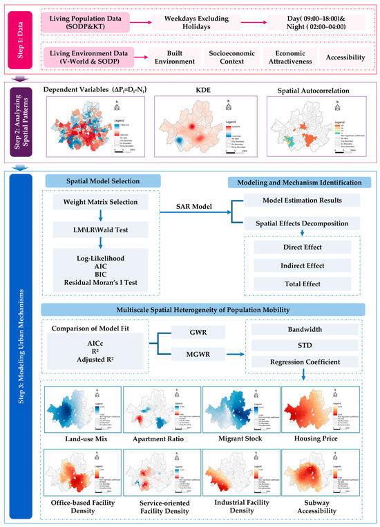
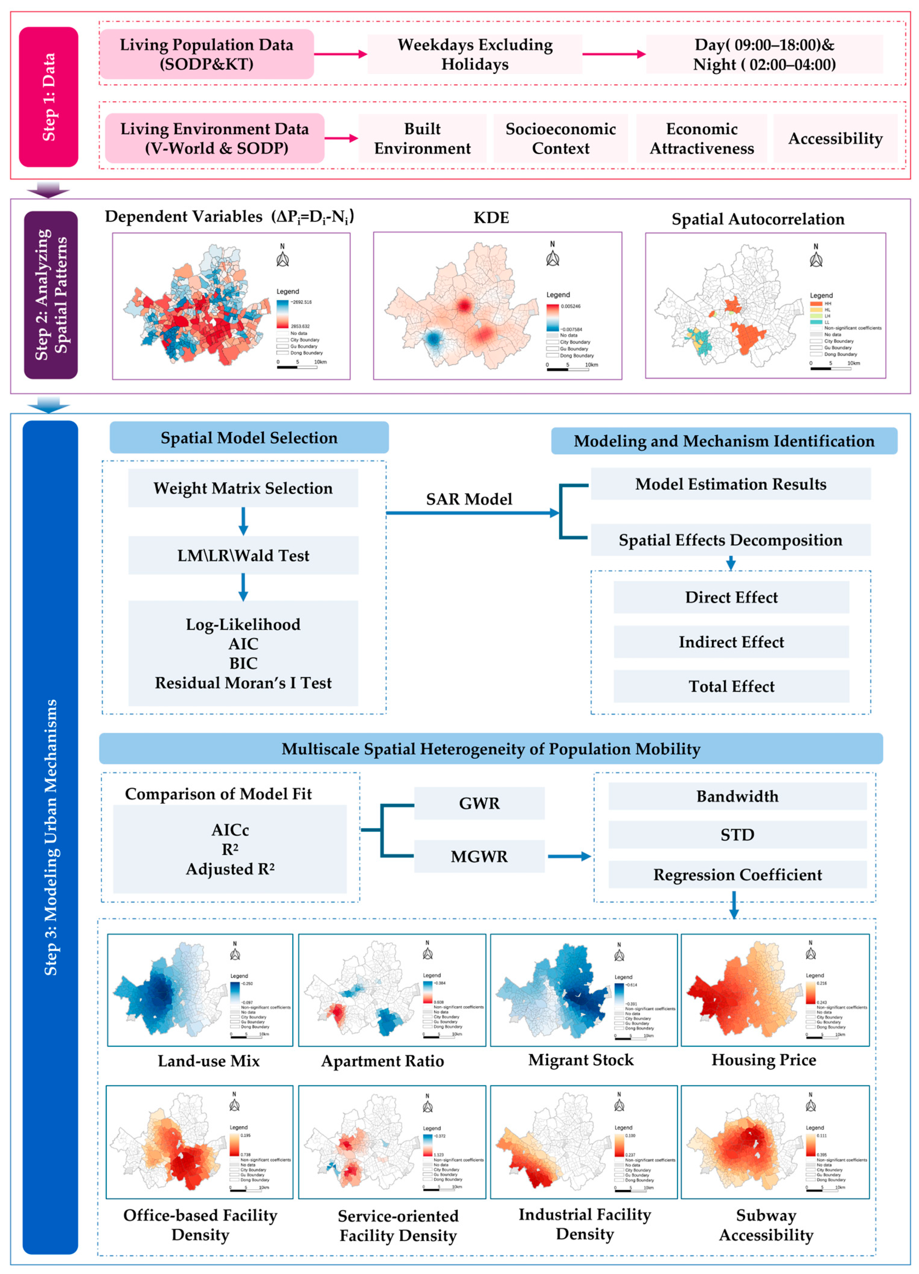
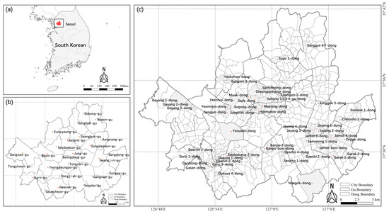
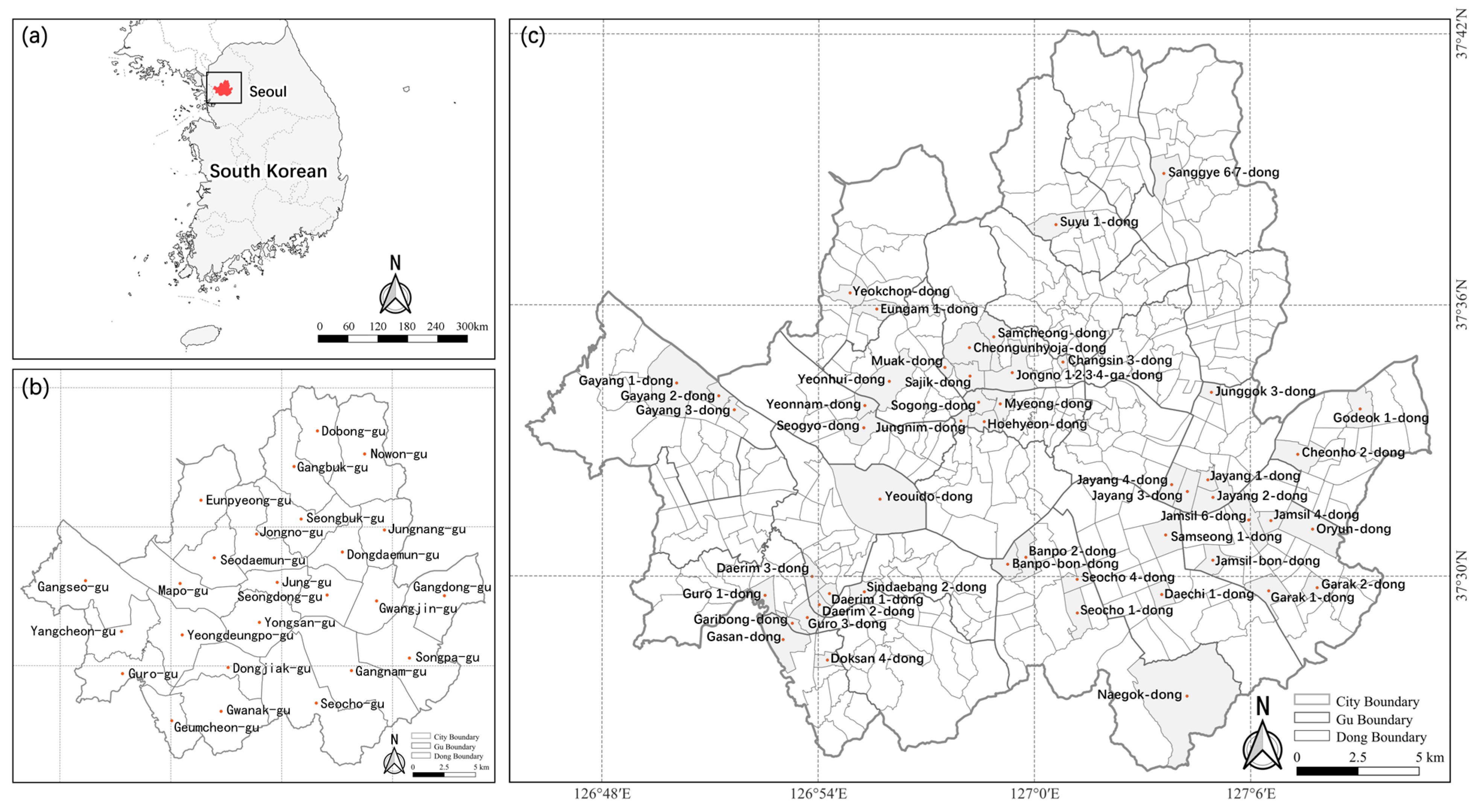
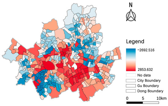
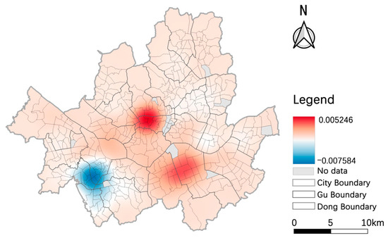
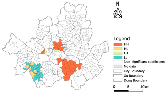
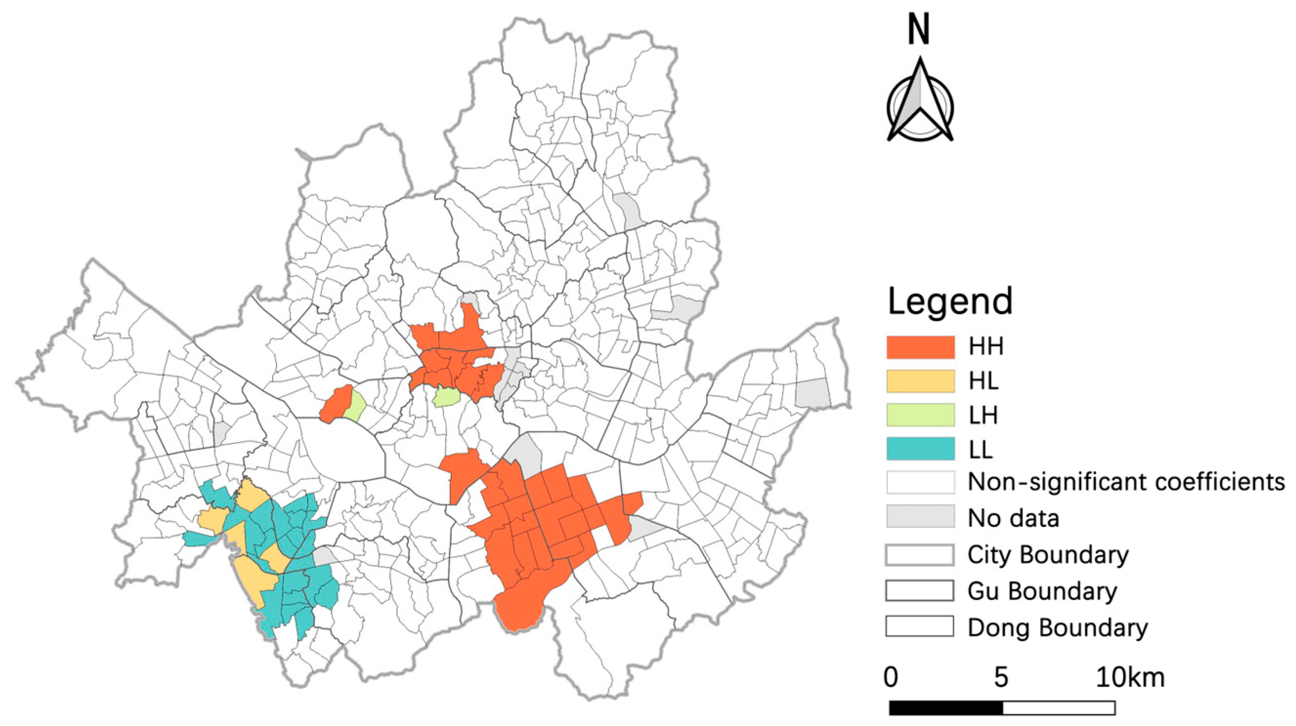
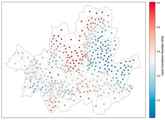
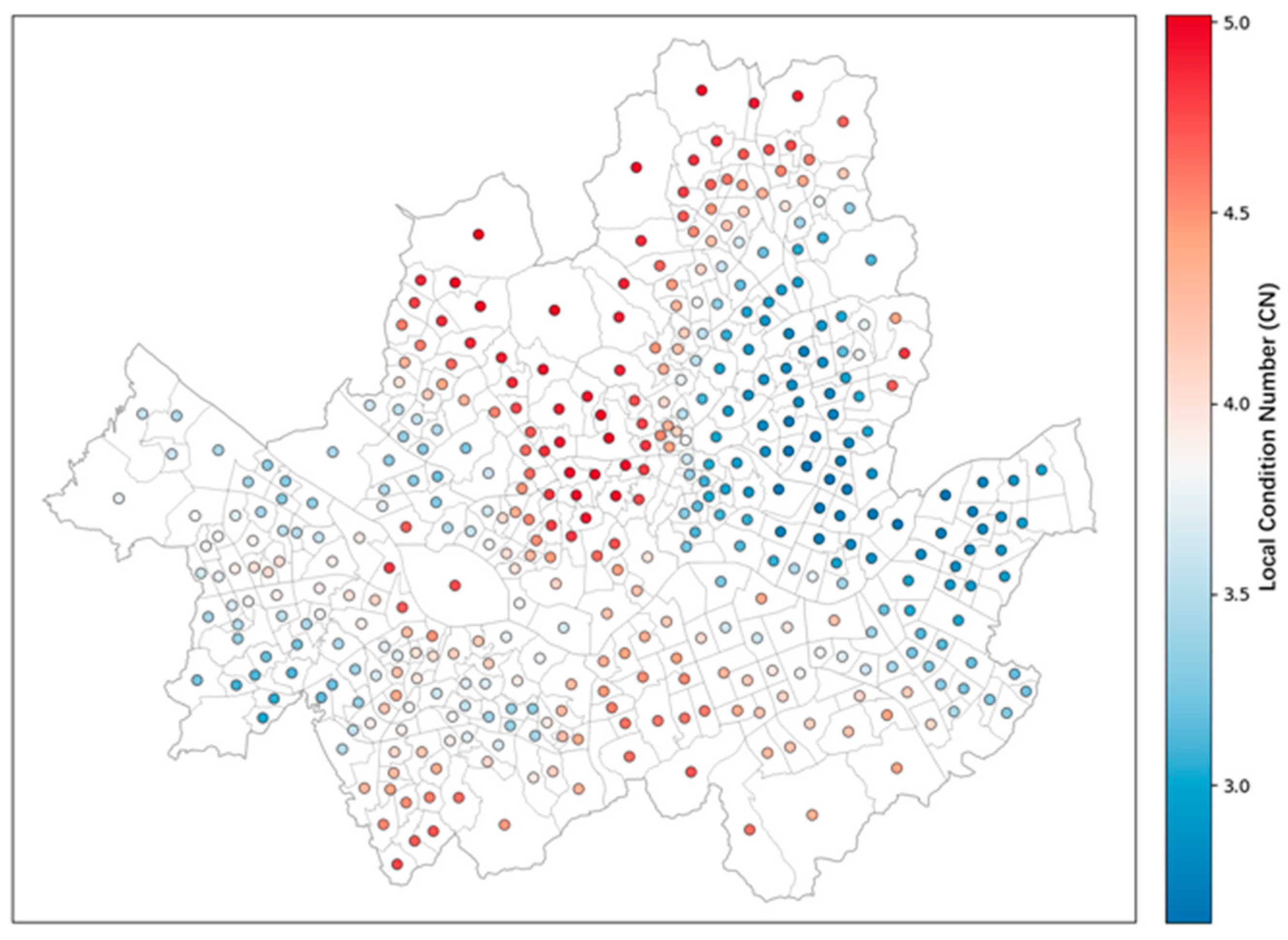
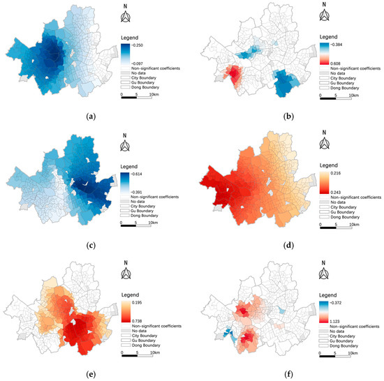
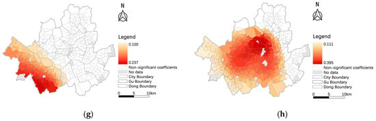
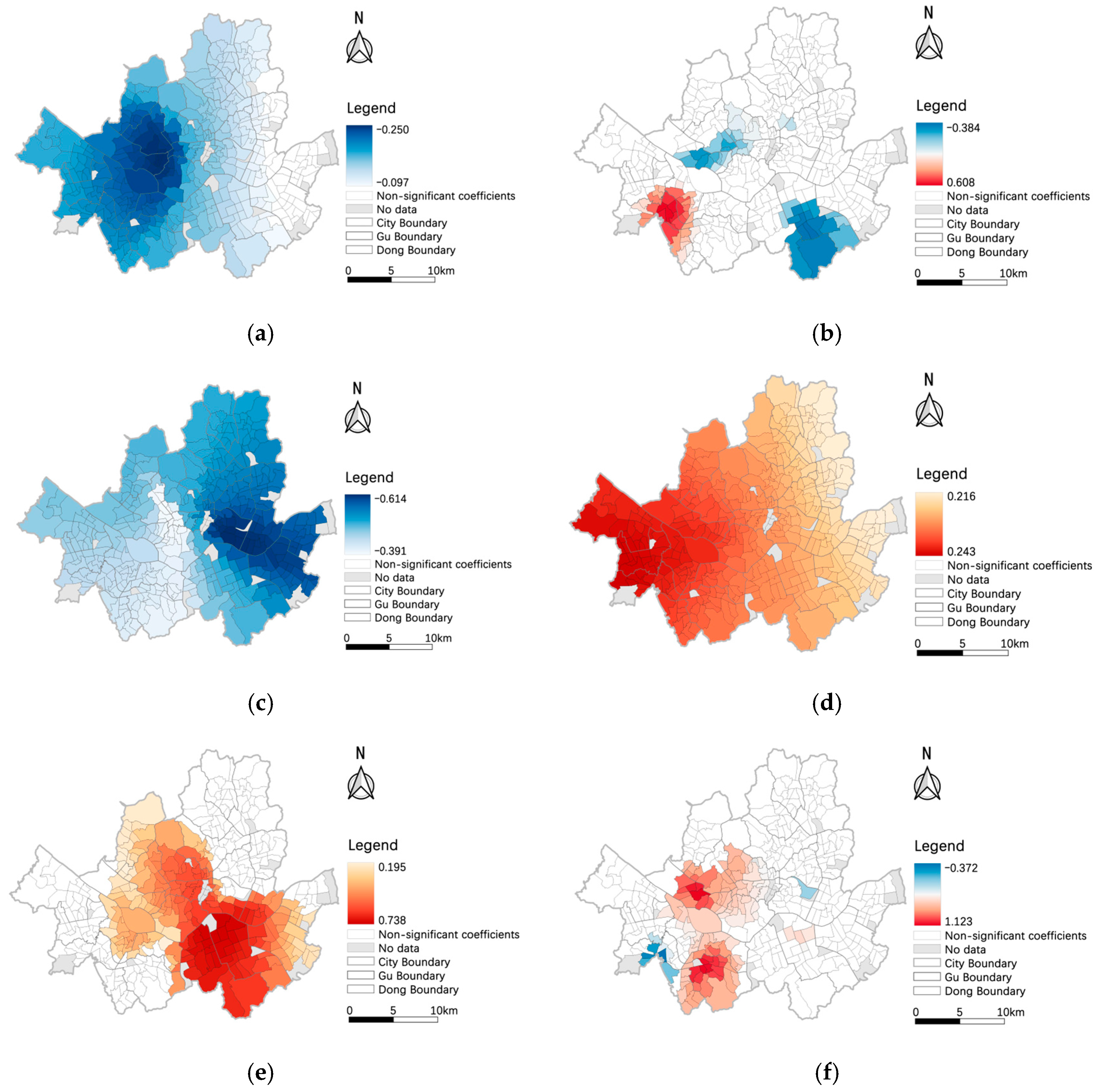
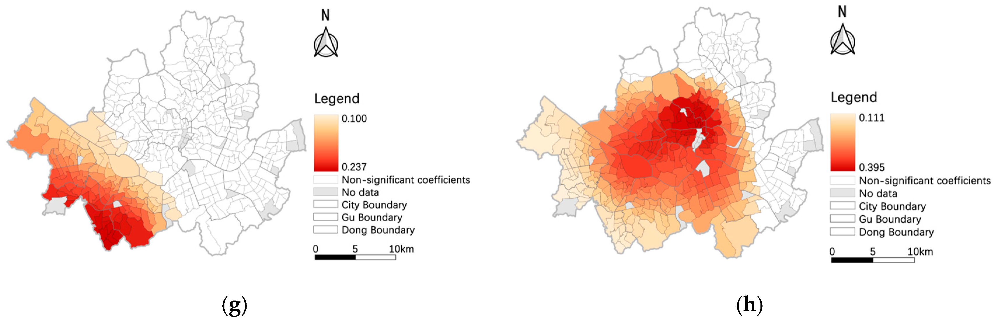

Disclaimer/Publisher’s Note: The statements, opinions and data contained in all publications are solely those of the individual author(s) and contributor(s) and not of MDPI and/or the editor(s). MDPI and/or the editor(s) disclaim responsibility for any injury to people or property resulting from any ideas, methods, instructions or products referred to in the content. |
© 2026 by the authors. Published by MDPI on behalf of the International Society for Photogrammetry and Remote Sensing. Licensee MDPI, Basel, Switzerland. This article is an open access article distributed under the terms and conditions of the Creative Commons Attribution (CC BY) license.