


Abstract
Recent advances in land system research depend heavily on efficient access to large-scale, multi-source remote sensing spatiotemporal databases. Although Text-to-SQL provides natural language interfaces, the scale and spatial complexity of remote sensing schemas generate significant noise for large language models, increasing inference costs and latency. This study presents graph-enhanced retrieval for accurate schema pruning (GRASP), a graph-based framework for schema pruning in remote sensing information systems. GRASP frames schema pruning as a semantic retrieval task and constructs a heterogeneous graph that represents both question semantics and database structure. By integrating a relation-aware transformer, a relational graph attention network, and pre-trained BERT representations, GRASP enhances schema understanding and supports joint table-column prediction through entity-level cross-attention. A dual-task objective combining contrastive learning with dynamic-threshold prediction mitigates class imbalance, while database value sampling and demonstration retrieval optimize inference performance. Experiments show that GRASP substantially improves schema pruning in spatiotemporal query scenarios: a 7B open-source LLM with GRASP surpasses an unaugmented 32B model on Spider; meanwhile, the framework also yields promising results on SpatialSQL, achieving a favorable balance among accuracy, cost, and deployment flexibility. GRASP provides a practical pathway for interdisciplinary researchers to query remote sensing databases in natural language, aiding spatiotemporal analysis.
1. Introduction
The continuous advancement of remote sensing technology has greatly improved our ability to observe and understand the Earth’s surface [1]. Massive, multi-source Earth observation data, including multispectral imagery, land-cover change records, and high-precision spatiotemporal indices, form the foundation of modern remote sensing information systems and support studies of urban expansion, agricultural yield, natural disasters, and ecosystem change [2].
The value of remote sensing big data for land system research depends heavily on efficient access to database content. In practice, remote sensing data are usually stored in large-scale spatiotemporal databases with complex schemas. A typical remote sensing information system may contain tens to hundreds of tables, such as image metadata tables, spatiotemporal index tables, and thematic result tables, with hundreds or even thousands of attributes [3]. Although such schema designs provide strong organizational capacity, they also create major barriers to data access. Domain experts, such as ecologists, urban planners, and agronomists, often lack structured query language (SQL) expertise, whereas database engineers are usually unfamiliar with the semantics of remote sensing data. This mismatch has become a major obstacle to broader participation in land system big-data research.
Natural language interfaces to databases, especially Text-to-SQL systems, provide a promising solution to this challenge [4,5]. By translating natural language questions into executable SQL queries, Text-to-SQL enables interdisciplinary researchers to access remote sensing spatiotemporal databases directly. Recent advances in large language models (LLMs) have created new opportunities for this task [6,7]. In this context, LLM-based Text-to-SQL offers a novel computational approach to facilitate spatiotemporal analysis in the artificial intelligence era, lowering the technical barrier to data access for land system research.
However, applying Text-to-SQL to remote sensing databases is substantially more difficult than in general benchmark settings. Remote sensing schemas are often much larger than those in standard datasets and contain many spatial and temporal attributes with highly similar semantics. Meanwhile, additional information must be incorporated into the context to inject domain-specific knowledge and other relevant details. When full schemas are provided to LLMs, excessive irrelevant context introduces substantial noise, reduces SQL generation accuracy, and increases inference cost and latency, thereby limiting deployment in practical remote sensing information services [8].
To address this issue, existing studies have explored schema pruning methods, including cross-encoder classifiers and dense retrievers based on bidirectional encoder representations from transformers (BERT)-class models. However, most existing methods treat database schemas as serialized text and do not explicitly model the graph-structured nature of remote sensing databases, where tables are linked by foreign keys, spatial associations, and temporal relationships. As a result, they have limited ability to capture the correspondence between question semantics and schema structure, especially in large and complex remote sensing scenarios.
To overcome these limitations, graph-enhanced retrieval for accurate schema pruning (GRASP) is proposed for schema pruning in natural language query interfaces to remote sensing spatiotemporal databases. GRASP follows a retrieve-then-generate paradigm and models schema pruning as a graph-enhanced semantic retrieval task. By integrating question semantics with database relational structure, the proposed framework identifies query-relevant tables and columns while filtering out irrelevant schema elements, thereby providing downstream LLMs with a compact and low-noise schema context.
As illustrated in Figure 1, conventional paradigms (the baseline pipeline) overwhelm the LLM with excessive irrelevant context, leading to hallucinated joins and reduced SQL generation accuracy. In contrast, the GRASP framework (the proposed pipeline) acts as a precise structural filter, thereby improving SQL generation performance while mitigating inference cost and latency in practical remote sensing information services.
Figure 1.
Baseline vs. GRASP schema context in remote sensing Text-to-SQL.
The main contributions are summarized as follows:
- (1)
- A graph-enhanced schema pruning framework, termed GRASP, is developed for natural language querying in remote sensing information systems. The framework introduces a retrieve-then-generate paradigm that couples a graph-enhanced discriminative pruner with an LLM-based generative decoder, achieving a favorable balance among performance, cost, and deployment flexibility. Unlike prior graph-enhanced methods that target end-to-end SQL generation, GRASP is positioned as a schema-pruning module within this pipeline, and is orthogonal to end-to-end Text-to-SQL optimizations such as LLM fine-tuning, self-correction and majority voting, which can be integrated with GRASP in a complementary manner.
- (2)
- A hybrid representation architecture is designed to jointly model semantic and structural information in complex database schemas. By combining relation-aware transformer (RAT) and relational graph attention network (RGAT), the framework captures both relational dependencies and heterogeneous graph topology for more accurate schema representation.
- (3)
- An entity-level prediction mechanism is introduced for joint table-column selection, together with a dual-task training strategy that combines contrastive learning and dynamic-threshold prediction to alleviate class imbalance in schema pruning.
- (4)
- Extensive experiments on the Spider benchmark and the SpatialSQL dataset demonstrate the effectiveness of GRASP in both general and remote sensing-specific scenarios. Under matched LLM backbones, GRASP consistently outperforms representative schema-linking/pruning baselines as well as graph-enhanced end-to-end methods. A 7B open-source LLM enhanced by GRASP achieves higher SQL execution accuracy than an unaugmented 32B model, indicating its practical value for deployment in computationally constrained environments.
The remainder of this paper is organized as follows. Section 2 reviews related work on Text-to-SQL, graph-based schema modeling, retrieval-augmented generation, and natural language interfaces for spatiotemporal databases. Section 3 presents the proposed GRASP framework in detail. Section 4 describes the experimental setup and reports the pruning results, ablation results, end-to-end SQL generation results, case study, and discussion. Section 5 concludes the paper and outlines directions for future work.
2. Related Work
2.1. Evolution of Text-to-SQL Methods
Text-to-SQL semantic parsing has progressed through multiple phases. Early methods transitioned from rule-based template matching to deep learning-driven neural network approaches. These methods include sequence-to-sequence models [9,10], sketch-based slot-filling approaches like SQLNet [11] and RYANSQL [12], and syntax-tree-guided decoders such as SyntaxSQLNet [13]. While these approaches significantly improved generation accuracy, they primarily treated the database schema as serialized text input, overlooking its inherent structural properties and failing to model inter-table relationships and hierarchical schema organization explicitly.
As researchers recognized the inherent graph structure of database schemas, graph neural networks were gradually integrated into this field. The current paradigm utilizes prompting strategies with LLMs to drive SQL generation. Inspired by retrieval-augmented generation (RAG), this approach adopts a two-stage pipeline. Schema pruning or demonstration selection is initially conducted using prompt engineering or dense vector retrieval, followed by final SQL generation by an LLM. This separation of schema linking from SQL generation enhances modularity, enables flexible component composition, and offers better context for utilizing the in-context learning capabilities of LLMs.
2.2. Graph-Structured Neural Networks for Text-to-SQL
Graph-structured neural networks have become a core technology for Text-to-SQL systems, used for encoding database schemas and modeling question–schema interactions. The basic idea is that relational databases naturally exhibit a graph structure: tables and columns act as nodes, while foreign keys, primary keys, and table-column relationships serve as edges. Such a structure can thus be naturally formulated as a heterogeneous graph [14].
In schema graph encoding, Global-GNN [15] models the database schema as a graph, with tables and columns as nodes, and foreign keys, primary keys, and related constraints as edges. It uses a gated graph neural network (GGNN) to propagate information across the schema graph, creating structure-aware node representations. RAT-SQL [16] introduced the RAT mechanism, which represents the input as a joint sequence of question tokens and schema elements and encodes pairwise relations using a relation matrix. Subsequent works, including SADGA [17] and ShadowGNN [18], adopted this design principle. RASAT [19] integrates relation-aware self-attention into the pre-trained T5 model, fusing structured relational information in a serialized manner. GRL-SQL [20] extends RAT’s single-hop relational encoding, forming SQL-GREASE layers inserted between the encoder and decoder of T5. GEG [21] adapts LLMs for graph-structured inputs through structure embedding injection, enhancing the self-attention mechanism with three types of graph structural information.
Graph neural networks represent a complementary line of research on graph-structured architectures. GADESQL [22] imports the RGAT originally proposed by Wang et al. [23] for sentiment analysis, applying it to database structure encoding and schema linking in Text-to-SQL. Graphix-T5 [24] further injects graph-aware layers into the T5 model, integrating RGAT blocks within each encoder layer for structure encoding. SGU-SQL [25] employs RGAT to encode both the query graph and schema graph, thereby establishing structural awareness.
The joint use of RAT and RGAT has attracted growing interest. RGISQL [26] processes the interaction graph with BERT in the input module to generate node and edge embeddings. The encoder adopts an RGAT architecture. At the output stage, multiple RAT layers integrate the updated embeddings into a unified representation.
Despite significant advancements in schema encoding and question–schema interaction modeling, existing graph-structured neural network methods still exhibit key limitations: insufficient use of the rich semantic knowledge embedded in pre-trained models, lack of explicit schema pruning mechanisms that treat all schema elements uniformly, and a heavy reliance on abstract syntax tree (AST)-based decoders that directly train compact models for end-to-end SQL generation, neglecting the in-context learning capabilities of LLMs. On the other hand, fine-tuning LLMs directly incurs prohibitive costs and hinders generalization ability.
2.3. Retrieval-Augmented Generation and Text-to-SQL
Retrieval-augmented generation [27] is a powerful paradigm that enhances language models by retrieving relevant external information. A RAG system typically comprises two components: a retriever, which identifies relevant documents given a query, and a generator, which produces output conditioned on both the query and the retrieved content. RAG’s success in open-domain question answering and knowledge-intensive tasks [28] has inspired its use in structured prediction tasks. In Text-to-SQL, the retrieval paradigm provides an effective approach for schema pruning: schema elements are treated as retrievable items, the natural language question serves as the query, and contrastive learning helps identify query-relevant tables and columns.
Recent research explores retrieval mechanisms for Text-to-SQL, focusing on two main directions: schema pruning and demonstration retrieval. In schema pruning, RESDSQL [29] proposed a ranking-enhanced encoding framework. A RoBERTa-based cross-encoder computes relevance scores for tables and columns, and top-ranked schema elements are passed to a seq2seq encoder to reduce noise from irrelevant entries. RB-SQL [30] applies separate dense retrieval models for table retrieval, column retrieval, and SQL pattern retrieval, retaining schema elements whose similarity exceeds a predefined threshold. DCG-SQL [31] uses a RoBERTa-based cross-encoder as a binary classifier to independently predict the relevance of each table and column with respect to the input question.
Under prompt engineering frameworks, LLMs possess a degree of general-purpose natural language processing capability that can be directed toward autonomous schema pruning. DIN-SQL [32] focused on decomposing the complex Text-to-SQL task into smaller sub-tasks, addressing schema linking through a prompt-based approach. C3 [33] adopted a clear prompting strategy to instruct the language model to first rank tables and columns by relevance to the question. Zhou et al. [34] systematically conducted a comparative evaluation of multiple prompting strategies, revealing that purely prompt-engineered approaches continue to face pronounced robustness challenges in cross-domain complex query settings. These findings further underscore the necessity of explicit schema pruning mechanisms.
In the area of demonstration retrieval, DAIL-SQL [35] systematically investigated example selection and organization strategies for in-context learning, proposing a selection criterion that simultaneously accounts for question similarity and query structural similarity. SPS-SQL [36] adopts a different strategy: queries are pre-synthesized over the target database schema to construct an embedded reference pool, from which similar pre-synthesized queries are retrieved at inference time as few-shot demonstrations.
Despite demonstrating the efficacy of retrieval mechanisms for Text-to-SQL, each of the methods above has limitations. Existing retrieval-based approaches have limitations in schema structure modeling: most compute table and column relevance independently, underutilizing the hierarchical dependencies among schema elements. Furthermore, they fail to model or leverage the graph structure of database schemas, treating structural information as an afterthought in a serialized representation. Relying only on classification or contrastive learning introduces challenges, including positive-negative class imbalance and difficulty in threshold selection during inference.
2.4. Natural Language Interfaces for Spatiotemporal Databases
The need for intelligent natural language query interfaces to spatiotemporal databases has been widely recognized in remote sensing information systems. Early research explored keyword matching and rule-template-based methods for geographic queries [37]. However, these methods exhibit limited generalizability and incur high rule maintenance costs, rendering them unsuitable for the complex schemas of large-scale remote sensing databases.
Research on natural language interfaces to spatiotemporal databases has increasingly aligned with the geographic information systems (GIS) domain, leading to semantic parsing systems tailored for geospatial queries [38]. Nevertheless, the scarcity of annotated data has long confined research to small, domain-specific datasets, limiting model generalization.
The emergence of large language models has created new opportunities for Text-to-SQL over remote sensing spatiotemporal databases [39]. In geospatial natural language interfaces, Mansourian et al. [40] proposed ChatGeoAI, which leverages Llama 2 to translate natural language queries into executable PyQGIS scripts. This enables interdisciplinary researchers to perform geospatial analysis directly and demonstrates the potential of LLMs to lower technical barriers. Li et al. [41] constructed a comprehensive benchmark for LLM-generated structured spatial data outputs (GeoJSON), systematically comparing RAG, fine-tuning, and prompt engineering for structured outputs and identifying characteristic failure modes when models process spatially nested structures. Pierdicca et al. [42] integrated GPT-4 and DeepSeek-R1 into GIS workflows to automate the generation of Python spatial analysis scripts from natural language inputs. Their results reveal persistent limitations on tasks that require the model to coordinate multiple spatial filters or integrate several intermediate computations, indicating that LLMs remain fragile when expected to compose long reasoning chains over complex spatial schemas. This observation further motivates the need to supply LLMs with a compact, low-noise schema context. Wang et al. [43] introduced the SpatialSQL spatiotemporal dataset, whose database schema encompasses multi-source remote sensing storage structures. This work also conducted a systematic investigation of GPT-based Text-to-SQL methods for spatiotemporal databases, validating the feasibility of LLMs for geospatial query generation. In their analysis, foundational data such as administrative divisions and roads recur across spatial databases under identical or near-identical naming, causing LLMs to reference attributes from in-context examples. This exposes persistent limitations in disambiguating semantically similar attribute names and corroborates the critical value of precise schema pruning in reducing contextual interference.
Remote sensing spatial databases exhibit structural characteristics that distinguish them from general-purpose databases. First, spatial attribute fields are numerous and semantically near-identical, increasing ambiguity in schema linking. Second, temporal and spatial attributes are tightly coupled, forming complex spatiotemporal query semantics. Third, remote sensing databases often embed explicit or implicit spatial relationships that require the model to possess spatial relationship modeling capabilities. Existing general-purpose Text-to-SQL methods have not been optimized for these remote sensing-specific properties, resulting in limited performance in real-world remote sensing systems.
Overall, prior work has advanced Text-to-SQL along three largely independent directions: graph-structured neural networks, retrieval-augmented generation, and natural language interfaces to remote sensing spatial databases, yet no existing method systematically integrates all three. Graph-structured approaches confer structural awareness but lack explicit schema pruning and underutilize the in-context learning capabilities of LLMs. Retrieval-augmented methods introduce schema pruning and demonstration recall but overlook the graph-topological properties of database schemas, and still face challenges such as class imbalance and inference-time threshold selection. Remote sensing-oriented research has revealed the distinctive difficulties posed by large-scale spatial database schemas in terms of semantic disambiguation and relational structure modeling, challenges not yet addressed by general-purpose Text-to-SQL methods. Notably, since the advent of LLMs, research attention in the Text-to-SQL community has shifted appreciably toward LLM-centric mechanisms such as instruction fine-tuning, self-correction, and majority-voting sampling, leaving the graph-enhanced direction and the LLM-based direction largely separated. To address these gaps, we propose GRASP, a retrieve-then-generate framework that provides an efficient and practical solution for schema pruning in natural language interfaces to remote sensing spatiotemporal databases.
3. Materials and Methods
3.1. Problem Definition
Here, is the set of all tables in the database schema, where denotes the total number of tables; is the set of all columns across all tables; and is the set of database integrity constraints, specifically primary keys and foreign keys, which define structural dependencies among tables and columns. In the context of remote sensing information systems, the database schema is large-scale and structurally complex. A typical remote sensing spatial database encompasses multiple functional table categories, including spatiotemporal index tables and administrative division tables. The column set includes many spatial and temporal fields with similar semantics, which makes schema linking difficult. These characteristics render the schema pruning task for remote sensing spatial databases more challenging than general-purpose scenarios; accurate pruning is essential for ensuring the correctness of downstream SQL generation.
Formally, is the token sequence produced by tokenizing the natural language question, denotes the token in the sequence and is the total number of tokens. Given a natural language question and a database schema , the objective of the schema pruning task is to learn a mapping function .
The pruned schema subset must satisfy two core objectives: completeness, which requires that all tables and columns referenced in the ground-truth SQL statement are retained in , thereby ensuring the correctness of downstream SQL generation; and conciseness, which requires that be as compact as possible so as to minimize the cognitive burden and computational overhead imposed on subsequent models.
The schema pruning task is reformulated as a graph retrieval problem: given an input question , the goal is to retrieve from the candidate schema element set a semantically relevant subset. The retrieval process evaluates the relevance between the query and candidate schema elements. Contrastive learning and dynamic threshold prediction are used to improve decision boundaries in the semantic space. Explicit graph-structural modeling is further incorporated to capture topological dependencies among schema elements. Based on this formulation, GRASP is proposed as a unified schema pruning framework that integrates heterogeneous graph modeling, relation-aware encoding, and contrastive learning.
3.2. Overall Architecture
GRASP incorporates graph-structural information into the deep representation space of a pre-trained language model, allowing the model to leverage both pre-trained semantic knowledge and task-specific relational structure. Methods based only on pre-trained models capture semantic information well but lack explicit modeling of the database structure. Conversely, graph-structured neural network methods can encode structural information but fail to leverage pre-trained knowledge. GRASP integrates the advantages of both paradigms, improving both semantic understanding and structural modeling.
Figure 2 shows the overall architecture of GRASP, which includes five tightly coupled modules that together form an end-to-end pipeline from input to decision.
Figure 2.
Overall architecture of GRASP.
An overview of each module is given below; detailed technical descriptions are presented in the subsections that follow.
Heterogeneous Graph Construction Module. It models the natural language question and database schema as a heterogeneous graph containing multiple node types and edge types, laying the structural foundation for subsequent relation-aware encoding.
Relation-Aware Encoder Module. This module first serializes the graph structure into a linear sequence suitable for input to a pre-trained language model. The BERT-RAT encoder replaces the latter layers of BERT with RAT layers, achieving deep fusion of pre-trained knowledge and graph-structural information. This design allows RAT layers to enhance BERT’s intermediate representations with relational information, improving both semantic and structural representations.
Semantic Graph Propagation Module. It dynamically identifies implicit semantic associations from the attention weights produced by the RAT layers. The discovered semantic edges are added to the graph to form the enhanced heterogeneous graph . Local message passing is then performed over this augmented structure using the RGAT. RAT captures global semantic information, while the RGAT performs local structural refinement, and they complement each other.
Dual-Task Prediction Head Module. This module combines contrastive learning with dynamic threshold prediction. The InfoNCE loss optimizes the similarity distribution between the input question and schema elements, while dynamic threshold prediction estimates the optimal decision boundary conditioned on the characteristics of each individual query, enabling query-specific filtering.
Context Augmentation Module. At inference time, this module introduces database value sampling and demonstration retrieval, providing the downstream LLMs with data samples and few-shot examples to better utilize their in-context learning ability.
3.3. Heterogeneous Graph Construction
Heterogeneous graph construction is the first step in modeling both the natural language question and the database schema. The question and schema are represented as a heterogeneous graph , where denotes the node set, the edge set, and the set of relation types.
3.3.1. Node Definition
The node set includes three types: question tokens, tables, and columns.
Question token nodes are defined at token-level granularity, with each token produced by the tokenizer treated as a node. Table and column nodes correspond to schema tables and columns. During serialization, two markers, [TAB] and [COL], are used to indicate table and column boundaries. The hidden states at these positions represent the corresponding entities.
3.3.2. Relation Type Design
Relation type design is key to heterogeneous graph modeling. A total of 19 relation types were defined, covering interactions among the three node types, question tokens, tables, and columns. These include adjacency relations between question tokens, table–column membership, foreign-key relations, cross-graph links, and semantic edges, as listed in Table 1. Each relation type represents a specific type of interaction, allowing the model to learn different relation patterns.
Table 1.
Definition of relation types.
Q_DIST_2 captures 2-hop syntactic token dependencies, following SADGA [17]; longer-range distances are encoded continuously by the Distance Lookup Table and do not require additional discrete relation types. Multiple foreign keys between the same pair of tables produce multiple C_FOREIGN edges; T_FOREIGN records the existence of any foreign-key link at the table level. For composite foreign keys consisting of multiple column pairs, each constituent column pair introduces a separate C_FOREIGN edge, so a -column composite key produces such edges. Partial matching means that after subword tokenization, at least one question token is a prefix or substring of a table (column) name token, and vice versa.
3.3.3. Matrix Representation
For efficient computation, the heterogeneous graph was converted into a matrix representation. Let denote the total number of nodes.
The Relation Matrix records the relation type between each pair of nodes, where is the relation type index from node to node , taking values in . For node pairs with no explicit relation, is set to the DEFAULT index 15. It should be noted that the values stored in are relation type indices, not edge weights. They serve as lookup keys for the Relation Lookup Table , which maps each index to a learned embedding vector; the embedding, not the raw index, modulates the attention computation. Index 0 is reserved for the SELF relation (self-loop); DEFAULT is assigned index 15 rather than 0 to avoid conflating the absence of an explicit structural relation with a self-loop, thereby preventing semantic ambiguity. The ordering of indices 0–18 reflects the sequence of definition during framework development and carries no semantic or priority meaning.
The Distance Matrix stores the shortest-path length between every pair of nodes, precomputed with breadth-first search (BFS). Entry denotes the number of edges on the shortest path from to .
3.4. Relation-Aware Encoder
3.4.1. Serialization and Embedding
To better leverage BERT, we serialize the heterogeneous graph into a linear sequence. The serialization format follows Equation (1):
Here, [CLS] is placed at the beginning of the sequence, and its hidden state represents the entire sequence. [SEP] is the separator token distinguishing the question segment from the schema segment. denotes the question tokens; and denote the tokens of table and its -th column, respectively; and is the number of columns in table . [TAB] and [COL] are special markers added to the BERT vocabulary and trained jointly. Table and column representations are obtained from the hidden states at these markers. For instance, the table name concert_singer is tokenized into three sub-tokens, concert, _, and singer, but its representation is determined by the preceding [TAB] token. Since BERT uses WordPiece tokenization, the node-level relation matrix is expanded to the token level using broadcasting.
3.4.2. BERT-RAT Encoding
The GRASP encoder integrates RAT layers into the BERT pipeline, as illustrated in Figure 3.
Figure 3.
BERT-RAT encoding architecture.
The first layers of BERT are retained as the base encoder, while the final layers are replaced by RAT layers. This design enables RAT layers to enhance BERT’s intermediate representations with relational information. Pre-trained semantic knowledge and graph structure are jointly refined in deeper layers.
The output of the BERT prefix is defined as Equation (2):
where denotes the input embeddings, is the attention mask used to suppress padding positions, and is the output hidden state of the BERT prefix. Node-type embeddings are subsequently fused before the representation is passed into the RAT layers, as shown in Equation (3):
where denotes the hidden state after type-information fusion, and is a linear projection layer. in Equation (2) (with a tilde) denotes the BERT prefix output prior to type-information fusion; in Equation (3) (without a tilde) is the type-fused representation that serves as the input to the first RAT layer. These are two distinct intermediate states in the encoding pipeline.
3.4.3. Relation-Aware Self-Attention
Relation-aware self-attention explicitly incorporates structural relations and topological distances between nodes into the attention computation. When computing attention weights, the model considers semantic similarity, relation type, and shortest-path distance. A Relation Lookup Table and a Distance Lookup Table are introduced, enabling the model to learn independent representations for each relation type and distance value. Here, is the Relation Lookup Table that maps each relation type index to a learned -dimensional key embedding. For example, retrieves the embedding for the T_HAS_C relation (a table contains a column), and retrieves the embedding for the DEFAULT relation (no explicit structural link). is the Distance Lookup Table, and the value is a reserved index for node pairs that are disconnected in the heterogeneous graph, ensuring they receive a distinct learned representation rather than being conflated with distance-0 (self) pairs. Values through encode BFS shortest-path hop counts, where is a hyperparameter capping the maximum encoded distance, and distances exceeding are clamped to . Under the multi-head attention mechanism, the relation-aware attention score from position to position within each head is computed as in Equation (4):
where denotes the query vector at position , denotes the key vector at position , and is the scaling factor. is the relation type index and is the shortest-path length. Relational and distance encodings act as additive biases that modulate the overall attention scores while preserving the integrity of the original content-based attention. The RAT layers are initialized from the corresponding BERT layers. Relation and distance embeddings are initialized using Xavier initialization.
3.5. Semantic Graph Propagation
3.5.1. Semantic Edge Extraction
The attention weights produced by the RAT layers encode implicit semantic associations. The Semantic Edge Extraction module transforms these soft attention signals into discrete edge structures. These edges are then used for message passing in the RGAT layers.
The RAT layers produce multi-layer and multi-head attention weights, which are aggregated into a unified edge-importance measure. Attention weights from the last RAT layers are averaged for cross-layer aggregation, followed by cross-head aggregation by element-wise maximum, as formulated in Equation (5):
where is the final aggregated attention matrix, indexes the attention head, and denotes the attention weights of head at layer of the RAT stack. Taking the maximum across heads preserves salient semantic associations identified by individual heads, avoiding dilution caused by averaging.
A decision boundary is introduced to convert aggregated attention values into edge-existence probabilities. A learnable threshold-based probability mechanism is defined, as shown in Equation (6):
where denotes the probability of a semantic edge existing between nodes and ; is the value of the aggregated attention matrix at position ; is a learnable threshold parameter that controls extraction sensitivity; is a temperature hyperparameter governing the steepness of the sigmoid function; and is the sigmoid function mapping real values to .
The downstream RGAT layers require discrete edge structures, whereas the computed edge probabilities are continuous. To bridge this gap, the straight-through estimator (STE) is adopted. This approach preserves end-to-end differentiability through forward discretization and backward continuity. Semantic edges are extracted only for question–question, question–table, and question–column pairs. Intra-schema and reverse-direction edges are excluded to align with the schema pruning objective. The dynamically added edges are integrated into the graph to form the enhanced heterogeneous graph , which is used for semantic graph propagation.
3.5.2. Relational Graph Attention Network
The enhanced heterogeneous graph combines the original graph with semantic edges. The goal of relational graph attention network is to perform local neighborhood aggregation over the enhanced heterogeneous graph , refining node representations by propagating information along explicit structural and semantic edges. This local message-passing operation is complementary to the RAT layers, which compute global sequence-level attention: while RAT captures long-range dependencies across all nodes simultaneously, RGAT captures fine-grained local structural context through edge-conditioned message passing, as illustrated in Figure 4.
Figure 4.
Overview of the semantic graph propagation.
The inputs to the RGAT are the hidden states produced by the RAT encoder, the Edge Mask , and the Semantic Edge Probability . The enhanced graph preserves the complete structural information of table–column, column–column, and table–table relationships within the schema, while additionally incorporating the dynamically learned question–schema semantic associations.
The representation of node at the RGAT input layer is , and its neighbor set in is . The RGAT computes the contribution of each neighbor to node using an attention mechanism. Query vector , key vector , and value vector are obtained through linear transformations. The raw attention score is then computed for node over neighbor . The edge probability extracted by the semantic edge module serves as a soft attention mask to modulate the attention scores, as described in Equation (7):
where is the binary edge decision; only connected edges participate in message passing. After normalization, produces the final attention weight . The updated node representation is computed through weighted aggregation of neighbor information. The updated representation of node within a single attention head is given by Equation (8):
where is the value vector of node in that attention head. A multi-head attention mechanism improves the expressive capacity of the RGAT. Multiple layers are stacked to enlarge the receptive field of message passing.
3.6. Dual-Task Prediction Head
The dual-task prediction head acts as the decision layer of GRASP, converting encoder-derived node representations into relevance scores for tables and columns, as illustrated in Figure 5.
Figure 5.
Overview of the dual-task prediction head.
A dual-task framework combines contrastive learning with dynamic threshold prediction, jointly optimizing representation quality and decision boundaries. Contrastive learning models relate relationships among samples, whereas dynamic threshold prediction adapts the decision boundary to each query. Relevance is determined based on the cosine similarity between the question and schema representations.
3.6.1. Entity Representation Extraction
As described in Section 3.4, BERT tokenization may split table and column names into multiple sub-word tokens, with the relation matrix broadcast to cover all token positions. Accordingly, the RGAT output is defined at the token level, where is the sequence length. Since schema pruning operates at the entity level, token representations are aggregated into entity representations for cross-attention and similarity computation.
The question representation is obtained by aggregating multiple token representations into a single vector. Let denote the index set of question tokens, and the corresponding hidden states. Weighted aggregation is performed using a self-attention mechanism, as given in Equation (9):
where is a multi-head self-attention layer that captures the relative importance of question tokens. The output is mean-pooled and passed through a two-layer projection, producing the final question representation vector .
Table and column representations are extracted by exploiting the serialization design introduced in Section 3.4. The [TAB] and [COL] boundary markers are positioned at the onset of each corresponding entity name. After encoding, the hidden states at these markers aggregate information from subsequent tokens and represent the semantics of the entire entity. The hidden states at [TAB] and [COL] positions are therefore used directly as the table entity representation and the column entity representation , respectively.
3.6.2. Entity-Level Cross-Attention
Database schemas possess an inherent hierarchical structure: columns belong to tables, and tables are interconnected through foreign keys. Although RAT and RGAT capture token-level dependencies, they do not explicitly model entity-level hierarchical structure. As shown in Figure 5, cross-attention introduces explicit hierarchical interactions among entity representations, enabling more structured schema reasoning. Three interaction components are included.
Column-to-table aggregation integrates information from constituent columns into each table. Let denote the set of child columns belonging to table . Column information is aggregated into each table using cross-attention, as formulated in Equation (10):
where serves as the query, and the representations of the child columns serve as keys and values. is the resulting aggregated column information. A gating mechanism is introduced for adaptive fusion, as formulated in Equation (11):
where denotes concatenation, are the gating weights, and denotes element-wise multiplication. The gating mechanism produces a coefficient vector in [0, 1] to control the contribution of aggregated information.
Table-to-column propagation allows each column to acquire context from its parent table. Column semantics depend not only on the column name itself, but also on the broader context of the table to which it belongs. For example, the column value carries different meanings in a spectral signature table versus a topographic feature table. Table-to-column propagation is computed using the same gated fusion scheme.
Question–schema interaction treats the question representation as the query, with the hierarchically refined table and column representations, organized as the schema sequence , serving as keys and values. Cross-attention extracts schema information relevant to the question, and gated fusion produces the refined question representation . This allows the question representation to absorb relevant semantic signals from the refined schema elements. Cosine similarity is used to quantify relevance between the question and schema elements.
3.6.3. Dynamic Threshold Prediction
Conventional methods rely on a fixed threshold to partition positive and negative samples. Because query difficulty varies substantially, a fixed threshold is insufficient. To address this limitation, the decision boundary is predicted dynamically for each query. The model attends to all candidate entity representations conditioned on the question, producing a scalar threshold. The practical impact of dynamic thresholding is two-fold. For complex queries referencing many schema elements, the predicted is calibrated lower, improving recall and preventing suppression of required schema elements. For simple queries referencing a few elements, is calibrated higher, improving precision by excluding irrelevant schema elements. This query-adaptive calibration is jointly enforced by the contrastive loss and the Separation Margin Loss. The dynamic threshold prediction for tables is formulated as in Equation (12):
where denotes the attention-weighted aggregation of all table representations conditioned on the question representation. is the aggregated vector, allowing the question to attend to the distribution of all candidate entities. maps the aggregated vector to a scalar, and constrains the threshold to the interval , consistent with the range of cosine similarity. The column threshold is computed analogously. At inference time, table is considered relevant when its similarity score , and column is predicted as relevant when .
3.6.4. Dual-Task Training Objective
GRASP adopts a dual-task training objective that combines a contrastive learning loss with a threshold loss. The contrastive loss optimizes the similarity distribution between the question and schema elements, while the threshold loss ensures that the predicted threshold effectively separates positive from negative samples. The two losses act in concert, jointly targeting representation learning and decision boundary calibration.
For table relevance prediction, let denote the positive sample set (tables referenced in the ground-truth SQL) and the negative sample set (unreferenced tables). The InfoNCE loss is defined as in Equation (13):
where is the number of positive samples, is the similarity score for the table , and is a temperature hyperparameter controlling the sharpness of the softmax distribution.
The InfoNCE loss for column relevance, , is defined analogously. The total contrastive loss is the sum of the table and column losses, as given in Equation (14):
The threshold separation loss constrains the predicted threshold so that it effectively separates positive from negative samples. A Separation Margin Loss is employed to achieve this objective, which comprises two components targeting recall and precision, respectively. The recall loss is defined in Equation (15):
where is the positive sample set, is the predicted threshold, is the similarity score of positive sample , is the margin hyperparameter, and is the rectified linear unit. A positive loss occurs when , i.e., , indicating that the threshold is too high and positive samples risk being missed. thus penalizes the scenario in which the threshold is so high that positive samples are not recalled.
The precision loss is defined in Equation (16):
where is the negative sample set and is the similarity of negative sample . penalizes the scenario in which the threshold is so low that negative samples are falsely recalled.
The dual-boundary design ensures that the threshold maintains sufficient separation between positive and negative samples. When the two distributions overlap, the loss encourages the model to learn improved representations so as to increase separability.
The total threshold loss is . The overall training objective is the weighted combination of the contrastive loss and the threshold loss, as given in Equation (17):
where is the weighting coefficient for the threshold loss. The contrastive loss constitutes the primary training signal, responsible for learning high-quality question and schema representations, while the threshold loss serves as an auxiliary task that learns appropriate decision boundaries on top of those representations.
3.7. Context Augmentation
Few-shot learning significantly improves LLMs’ performance on Text-to-SQL tasks. At inference time, two context augmentation strategies are applied to leverage the in-context learning capability of LLMs.
Database value sampling augments the prompt with concrete data instances, allowing the LLMs to capture the underlying content and schema format more effectively. For each selected table, the first rows are obtained deterministically via a SELECT LIMIT query and appended to the schema description; under SQLite, in the absence of an ORDER BY clause, the returned rows follow the internal storage order, so the sampling result is reproducible across runs on the same database file.
Demonstration retrieval selects semantically similar examples from the training set before SQL generation. Each training sample is stored in a demonstration pool, including the question text and its vector representation, the ground-truth SQL, and the pruned schema with sampled values. During inference, the most similar samples are retrieved based on vector similarity to the input question. The retrieved examples are formatted as a few-shot prompt and provided as context to the LLMs. This encourages the model to follow SQL generation patterns from similar questions.
4. Experiments
This section presents a systematic empirical evaluation of GRASP on benchmark datasets to validate the proposed method from two complementary perspectives: the schema pruning stage, which evaluates accuracy and recall in filtering irrelevant schema elements; and the SQL generation stage, which examines how the pruned schema affects execution accuracy of SQL queries generated by large language models.
4.1. Experimental Setup
4.1.1. Datasets
To thoroughly evaluate the performance of the GRASP method, we selected two representative datasets: the Spider dataset and the SpatialSQL dataset.
- Spider Dataset. The Spider dataset [44] was adopted as the primary evaluation benchmark throughout development. Spider is a large-scale, cross-domain Text-to-SQL benchmark in which the training, development, and test splits contain non-overlapping database schemas, enabling a strict evaluation of model generalization to unseen databases. Its multi-domain and multi-table schema structure closely reflects the complexity of remote sensing spatial databases, facilitating the evaluation of model generalization and cross-database transferability. Several domains within Spider involve spatiotemporal concepts, providing partial coverage of query patterns relevant to remote sensing applications. Moreover, large-scale annotated spatiotemporal Text-to-SQL datasets remain scarce [43], making Spider a necessary complement for rigorous model development and ablation analysis. Experimental results on Spider thus provide a reliable indicator of GRASP’s schema pruning capability under complex schema conditions.
- SpatialSQL Dataset. To further assess the applicability of GRASP in real-world remote sensing information system scenarios, experiments were additionally conducted on the spatiotemporal Text-to-SQL dataset constructed by Wang et al. [43]. The dataset is built on real geospatial data with annotated natural-language queries, and includes multiple geospatial databases from the tourism, transportation, education, and administrative-division domains, covering diverse and complex GeoSQL queries. Its database content is drawn from actual geospatial sources, and its schema design follows realistic remote sensing information management practice, providing an in-domain benchmark for evaluating schema pruning performance in remote sensing contexts.
4.1.2. Evaluation Metrics
For each sample , the ground-truth SQL s parsed to obtain the required table set and column set . The corresponding model predictions are denoted and . To comprehensively assess pruning quality, Precision (P), Recall (R), and F1 score are computed separately at both the table and column levels.
Recall measures completeness, specifically, whether the model successfully retains all tables and columns required by the ground-truth SQL. This is a prerequisite for correct downstream SQL generation. Table-level and column-level recall are respectively defined as:
Precision measures conciseness, indicating whether the model effectively eliminates irrelevant tables and columns. Higher precision implies fewer noisy tokens supplied to the LLMs, thereby reducing contextual overhead and inference-time interference. Table-level and column-level precision are respectively defined as:
F1 score is the harmonic mean of precision and recall, providing a unified measure of overall model performance:
For generated SQL, the predicted query is executed to produce a result set . It is considered correct if it matches the result set from the ground-truth SQL. Execution accuracy (EX) is defined as
where is the indicator function that equals 1 if the execution result set of the predicted SQL is identical to that of the ground-truth SQL under row-order-consistent, column-order-agnostic comparison, and 0 otherwise. To simulate real-world deployment with high query throughput, an inference timeout was applied. Predictions exceeding the timeout were treated as incorrect.
4.1.3. Configuration
The GRASP framework was implemented in PyTorch 2.4.1. The base encoder was BERT-base-uncased with its standard tokenizer and default configuration; context window extension [45] was applied for longer inputs. Hyperparameters were tuned on the validation set using grid search. The node-type embedding dimension was set to 64. The number of RAT layers was set to 2, with semantic edge extraction performed from the RAT attention weights. The number of RGAT layers was 3, with 4 attention heads. The entity-level cross-attention module comprised 3 layers with 8 attention heads. The dynamic threshold margin was 0.1, the threshold loss weight was 0.1, and the dropout probability was uniformly 0.2. The InfoNCE temperature was set to 0.07, following established practice in contrastive representation learning. In the semantic-edge sigmoid, the temperature was fixed at 0.5, selected via the validation-set grid search described above, and the learnable threshold parameter was initialized to 0.3 and updated jointly with the rest of the network. The straight-through estimator applied to the edge probabilities performs hard thresholding at 0.5 in the forward pass and propagates an identity surrogate gradient in the backward pass, preserving end-to-end differentiability. The maximum encoded distance in the Distance Lookup Table was set to 100. All experiments used a fixed random seed of 42, applied uniformly to PyTorch, NumPy, and the Python random module. Both the value sampling count and the demonstration retrieval count were set to 3.
During training, the AdamW optimizer was used. The learning rate for BERT parameters was set to , while that for all other modules, including RGAT, the prediction head, and additional components, was set to . The batch size was 4, with a gradient accumulation step of 8. Training proceeded for a maximum of 200 epochs under early stopping, based on the average F1 score over tables and columns on the development set, with a patience of 10 epochs. The pruning model was trained and evaluated on heterogeneous accelerator cards via the SCNet platform. Large language model inference was performed through the Siliconflow API. The inference timeout was set to 60 s. Demonstration retrieval was performed using the gte_sentence-embedding_multilingual-base model for vector encoding.
4.2. Individual Component Analysis
This section focuses on the filtering capability of the pruning model in isolation. A simplified baseline with frozen BERT weights was used as the starting point. Individual components were then incrementally introduced on the Spider development (Spider-dev) and test (Spider-test) sets to isolate their contributions. The effect of depth was further examined by varying the number of layers in key components.
4.2.1. Individual Component Validation
Using a frozen-BERT baseline as the starting point, a single component was added at a time: BERT fine-tuning, RAT, the RGAT semantic graph propagation module, entity-level cross-attention, or dynamic threshold prediction. These single-component experiments aim to evaluate the standalone effect of each component and do not reflect the optimal performance of the fully combined model; the combined gains and interaction effects are analyzed in the ablation study. Precision (P), Recall (R), and F1 scores at the table and column levels on the Spider-dev and Spider-test are reported in Table 2 and Table 3, respectively.
Table 2.
Individual component validation results on Spider-dev.
Table 3.
Individual component validation results on Spider-test.
BERT fine-tuning yields the most substantial and consistent improvement. On the Spider-dev, table F1 rises from 0.616 to 0.890 and column F1 from 0.343 to 0.721. A consistent trend is observed in the test set. These results suggest that static semantic similarity alone is insufficient for schema pruning. Fine-tuning is necessary to align the pre-trained language model with the target domain. It enables learning the mapping between natural language expressions and database schema naming conventions.
RAT layers also deliver meaningful gains even under frozen-BERT conditions. By injecting single-hop relational information and distance encodings through relation-aware attention, the encoder captures structural relationships more effectively during attention computation, improving the relevance ranking of tables and columns. The relatively modest improvement in column F1 attributable to RAT alone suggests that structural bias is insufficient to resolve fine-grained column discrimination; stronger semantic modeling or hierarchical interaction remains necessary.
Notably, RGAT in isolation yields only marginal improvement over the baseline. Under limited semantic separability, local message passing tends to propagate irrelevant information along noisy edges. This suggests that RGAT functions best as a structural refinement module built on high-quality initial representations, rather than replacing semantic modeling.
Entity-level cross-attention substantially improves recall through explicit hierarchical interaction, reducing the likelihood of missing elements required by the ground-truth SQL. However, when applied in isolation on a weak semantic representation, cross-attention results in low column-level precision. This indicates that hierarchical interaction improves coverage but introduces over-recall. The resulting noise requires suppression by a threshold mechanism or stronger representation learning.
Dynamic threshold prediction proves particularly effective for column selection, raising column F1 to 0.406 on the Spider-dev set, driven primarily by precision gains and a more robust decision boundary. This result shows that the number of relevant tables and columns varies significantly across queries. A fixed threshold is therefore inadequate to balance precision and recall. Query-adaptive threshold prediction mitigates the decision shift caused by class imbalance and varying query difficulty.
4.2.2. Effect of RAT Layer Count
The RAT layers are responsible for injecting graph-structural biases into the pre-trained language model. Pruning performance under varying numbers of RAT layers is illustrated in Figure 6.
Figure 6.
Effect of RAT layer count on pruning performance.
The model achieves optimal F1 scores for both tables and columns at a RAT depth of 2. Increasing the depth to 3 or 4 layers does not yield further improvement and instead leads to a slight decline. Under the current task scale, two RAT layers are sufficient to capture structural dependencies. Additional layers may disrupt the semantic coherence established by the BERT prefix and increase the risk of overfitting.
4.2.3. Effect of RGAT Layer Count
The RGAT layers are responsible for explicit message passing over the enhanced heterogeneous graph. Pruning performance under varying numbers of RGAT layers is illustrated in Figure 7.
Figure 7.
Effect of RGAT layer count on pruning performance.
Performance improves steadily as the RGAT depth increases from 1 to 3 layers, indicating that multi-hop message passing facilitates the aggregation of broader neighborhood context. Beyond 3 layers, however, performance plateaus or slightly degrades. Effective reasoning paths in the schema-enhanced graph are typically short. Excessively deep message passing leads to oversmoothing, causing node representations to converge and reducing their discriminability.
4.2.4. Effect of Cross-Attention Layer Count
Entity-level cross-attention is responsible for establishing explicit hierarchical interactions among table, column, and question representations. Pruning performance under varying numbers of cross-attention layers is illustrated in Figure 8.
Figure 8.
Effect of cross-attention layer count on pruning performance.
The results demonstrate that the cross-attention mechanism effectively balances information exchange between tables and columns. Shallower configurations cannot fully integrate the required information flows for column-to-table aggregation and table-to-column propagation. Deeper configurations increase training difficulty without proportional benefit.
4.3. Ablation Study
A detailed ablation study was conducted on both Spider-dev and Spider-test to evaluate the contribution of each core component in GRASP. The full model was used as the reference. Key modules were then removed or replaced in turn, and the resulting performance changes were recorded. The ablation configurations are defined as follows:
- Full Model (GRASP): The complete model includes BERT fine-tuning, 2 RAT layers, 3 RGAT layers, 3 cross-attention layers, and dynamic threshold prediction;
- w/o Dynamic Threshold: Dynamic threshold prediction is removed, and a fixed threshold of 0 is used;
- w/o Cross-Attention: The entity-level cross-attention module is removed; predictions are made directly from the RGAT output;
- w/o RGAT: The Semantic Graph Propagation module and RGAT layers are removed; only RAT encoding is retained;
- w/o RAT: The RAT layers are removed; the model reverts to standard BERT encoding;
- w/o BERT Fine-tuning: BERT parameters are frozen, and only the parameters of the RAT layers, the graph network, and the prediction head are trained.
Table 4.
Ablation study results on the Spider-dev.
Table 5.
Ablation study results on the Spider-test.
Freezing BERT parameters (w/o BERT Fine-tuning) leads to a sharp performance drop. On the Spider-test, table F1 falls from 0.935 to 0.781 and column F1 from 0.923 to 0.709. This result demonstrates that graph-oriented network architectures alone are insufficient to bridge the semantic gap between a pre-trained model and the target task. Schema pruning requires a nuanced understanding of the semantic mapping between natural language questions and database schema elements. Fine-tuning provides the mechanism for achieving this alignment.
Removing either the RAT layers (w/o RAT) or the RGAT layers (w/o RGAT) produces a notable performance decline. On the Spider-test, omitting RAT reduces table F1 by approximately 3.4%, confirming that injecting relational biases during encoding is essential for understanding schema topology. Omitting RGAT reduces table F1 by 3.5%. This indicates that explicit message passing over the semantically augmented graph effectively captures local structural context and refines node representations. The combination of RAT and RGAT consistently outperforms either component in isolation, confirming the complementarity of global sequence attention and local graph propagation.
Removing entity-level cross-attention (w/o cross-attention) lowers table F1 on the Spider-test to 0.914. The cross-attention module enriches table representations by aggregating column-level information and propagates table context to individual columns. The results indicate that explicit hierarchical modeling reduces missed elements and improves completeness in schema selection.
Removing dynamic threshold prediction (w/o dynamic threshold) primarily degrades recall and overall F1. On the Spider-test, table recall drops markedly from 0.928 to 0.885, and table F1 falls from 0.935 to 0.910. This confirms that both the number of relevant schema elements and prediction difficulty vary across queries. A fixed threshold is therefore either overly conservative or overly permissive. The dynamic threshold mechanism adaptively calibrates the decision boundary based on query complexity. This improves recall while maintaining high precision.
The ablation results confirm that each component of GRASP contributes a distinct and positive effect to overall performance. The components collectively form a robust pruning architecture that integrates deep semantic understanding with structural awareness.
4.4. Hyperparameter Sensitivity and Stability Analysis
The architecture-level hyperparameters (the numbers of RAT, RGAT, and cross-attention layers) are analyzed in Section 4.2, as they determine model capacity and inductive bias and therefore exert the largest qualitative effect on pruning behavior. The training-side hyperparameters, including the margin in the Separation Margin Loss and the threshold-loss weight in the overall training objective, were selected through validation-set grid search, as described in Section 4.1.3. This section reports the full grid-search results for and , which are the two training-side hyperparameters most directly tied to the dynamic-threshold mechanism, and additionally evaluates the stability of GRASP across random seeds. All experiments in this section follow the configuration of Section 4.1.3 except for the parameter under study.
The margin in the Separation Margin Loss (Equations (15) and (16)) controls the gap enforced between the predicted threshold and the similarity scores of positive and negative samples. Pruning performance under on Spider-dev and Spider-test is shown in Figure 9. retains the threshold loss but removes the explicit margin requirement; positive and negative samples are still pushed to the correct side of the threshold but no gap is enforced between them. Performance peaks at and declines for larger values, indicating that an excessively wide enforced margin over-constrains the score distribution and impedes representation learning. The grid search therefore selects .
Figure 9.
Effect of margin on pruning performance.
The weight in Equation (17) balances the contrastive loss and the threshold loss. Pruning performance under on Spider-dev and Spider-test is shown in Figure 10. Setting zeroes out the threshold loss, leaving the dynamic-threshold predictor in place at inference but without a dedicated training signal. Performance is highest at and decreases for both smaller and larger weights, indicating that the threshold loss is most effective as a lightweight auxiliary signal that complements rather than dominates the contrastive objective. The grid search therefore selects .
Figure 10.
Effect of threshold-loss weight on pruning performance.
To assess stability independent of any particular initialization, ten independent training runs were conducted without fixing the random seed. GRASP achieves table F1 of and column F1 of on Spider-dev, and table F1 of and column F1 of on Spider-test. This indicates that the observed improvements are not artifacts of any single random configuration. Taken together, the sensitivity analysis and the stability evaluation support the values of and identified by the grid search and the reliability of the reported gains.
4.5. Context Augmentation Analysis
At inference time, database value sampling and demonstration retrieval were introduced to exploit the in-context learning capabilities of large language models. To quantify the effect of these augmentation strategies on SQL generation, execution accuracy was compared across different configurations on the Spider-dev. These configurations include the baseline GRASP (no augmentation), value sampling only, demonstration retrieval only, and the full combination of both strategies. It should be noted that inference-time context augmentation is not the primary focus of the present work. The two basic augmentation mechanisms employed here are intended to assess whether large and small models can collaborate effectively under the proposed retrieve-then-generate paradigm, and whether the in-context learning capability of LLMs can further improve SQL generation quality. Context augmentation for LLMs remains a direction worthy of further investigation. The effect of augmentation strategies on EX across different LLM scales is illustrated in Figure 11.
Figure 11.
Effect of context augmentation strategies on Spider-dev.
Value sampling yields the most pronounced EX improvement, contributing gains of 2.3 percentage points and 1.5 percentage points on the 7B and 32B models, respectively. Incorporating actual database values into the prompt enables the model to more accurately infer the semantic meaning of individual columns. Demonstration retrieval, by supplying the SQL generation process for structurally similar questions as structured exemplars, guides the model in learning the generation patterns of complex query statements. The combination of both strategies achieves the best overall performance, indicating that the content-level awareness provided by value sampling and the pattern-level awareness provided by demonstration retrieval exhibit significant complementarity within the in-context learning framework.
4.6. SQL Generation Evaluation
This section evaluates the contribution of GRASP as a pre-generation pruning module to the end-to-end Text-to-SQL task. GRASP is compared against three groups of baselines: (i) the Full Schema baseline, in which the complete database schema is supplied directly to the LLMs; (ii) two representative schema-linking/pruning methods, DIN-SQL and C3, re-executed under identical LLM backbones to ensure a like-for-like comparison; and (iii) three graph-enhanced end-to-end Text-to-SQL methods, RAT-SQL+GAP+NatSQLG, RASAT+PICARD, and Graphix-3B+PICARD. EX on the Spider-dev and Spider-test is reported in Table 6 and Table 7, respectively.
Table 6.
Comparison of SQL generation EX on Spider-dev.
Table 7.
Comparison of SQL generation EX on the Spider-test.
Across both model scales, GRASP-pruned configurations substantially outperform the Full Schema baseline, yielding clear noise-reduction gains. On the Spider-test, EX improves by 7.7 percentage points for the 7B model and 4.8 percentage points for the 32B model. These results confirm that LLMs are susceptible to interference from irrelevant schema elements. By supplying a compact pruned schema, GRASP helps LLMs focus on task-critical information. This reduces hallucinations and incorrect table or column references.
Under matched LLM conditions, GRASP also consistently outperforms the two representative schema-linking/pruning baselines. On the Spider-test, GRASP-Qwen2.5-7B exceeds DIN-SQL by 5.8 percentage points and C3 by 4.6 percentage points; GRASP-Qwen2.5-32B exceeds DIN-SQL by 1.7 points and C3 by 1.8 points. Consistent improvements are observed on the Spider-dev. These results indicate that the gains of GRASP arise from its graph-enhanced pruning mechanism itself, rather than from differences in the underlying LLM. As a complementary practical advantage, the retrieve-then-generate pipeline of GRASP issues a single LLM call per query after offline pruning, whereas DIN-SQL requires multiple sequential LLM calls (schema linking, classification, generation, and self-correction), and C3 additionally relies on self-consistency sampling. GRASP-Qwen2.5-32B further surpasses the three graph-enhanced end-to-end baselines on both splits, exceeding RAT-SQL+GAP+NatSQLG, RASAT+PICARD, and Graphix-3B+PICARD by 9.1, 6.9, and 4.8 percentage points on the Spider-test, respectively.
A particularly notable finding is that Qwen2.5-7B augmented with GRASP achieves an EX of 77.9%, surpassing the 77.6% obtained by the unaugmented 32B model. This shows that lightweight, high-precision pruning enables a smaller LLM to match or exceed the performance of a larger model. The result validates the considerable practical potential of the retrieve-then-generate paradigm for real-world deployment. Because the Spider development and test splits use database schemas that are disjoint from the training schemas by construction, the consistent improvements observed across Spider-dev and Spider-test constitute direct evidence of zero-shot cross-database generalization of the graph retrieval-based paradigm.
To further assess the effectiveness of GRASP in remote sensing and geospatial database settings, experiments were conducted on the SpatialSQL dataset. We continued training the model pre-trained on the Spider dataset. Experiments followed the SSpa prompt format with three in-context demonstrations and used Dataset1. Following the standard SpatialSQL protocol, the first round used Ada and Edu as training data and Tourism and Traffic as test data. The second round reversed this assignment. Final performance was reported as the average over both rounds. For consistency with the Spider experiments, DIN-SQL and C3 are also evaluated on SpatialSQL under the same Qwen2.5-32B-Instruct and DeepSeek v3 backbones, alongside the DAIL-SQL baseline. Results are reported in Table 8.
Table 8.
Comparison of SQL generation EX on SpatialSQL.
On the SpatialSQL dataset, GRASP-pruned configurations again substantially outperform the Full Schema baseline across both model scales, delivering pronounced noise-reduction gains. Under the Qwen2.5-32B-Instruct backbone, GRASP achieves 63.5% EX, exceeding DAIL-SQL (61.0%, +2.5), DIN-SQL (56.5%, +7.0), C3 (54.0%, +9.5), and the Full Schema baseline (52.0%, +11.5). Under the DeepSeek v3 backbone, GRASP reaches 67.5%, with corresponding gains of +2.0, +5.5, +8.0, and +13.5 percentage points over the same set of baselines. This effect is particularly salient in the remote sensing domain. Geospatial spatiotemporal databases often contain many redundant attribute fields. Providing the full schema to an LLM introduces severe contextual interference and degrades SQL generation quality. GRASP uses graph-enhanced retrieval to precisely identify the tables and columns relevant to the query, effectively filtering out noisy fields in the remote sensing database. The results indicate that schema pruning provides greater benefits for smaller models. This has practical implications for on-device spatial SQL generation in resource-constrained environments such as remote sensing ground stations and edge platforms.
4.7. Case Study
A representative case is presented to illustrate the mechanism of GRASP. The input question was: “What is the total population of the districts whose areas are in the top 3?”
The database comprised three tables: the district table (containing fields such as District_ID, Area_km, and Population), the spokesman table (containing fields such as Spokesman_ID, Name, and Points, among others), and the junction table spokesman_district (containing Spokesman_ID, District_ID and Start_year). Only the Area_km and Population columns from the district table are required to answer this query.
Under the Full Schema condition, the LLM was misled by the presence of the spokesman_district table. It incorrectly inferred that accessing district data required a join through spokesman_district, imposing a database structural constraint on the query execution path. This hallucination introduced an irrelevant table into the JOIN chain, producing the following erroneous SQL:
SELECT SUM(T2.Population)
FROM spokesman_district AS T1
JOIN district AS T2 ON T1.District_ID = T2.District_ID
WHERE T2.Area_km IN (
SELECT Area_km FROM district
ORDER BY Area_km DESC LIMIT 3
);
Figure 12 illustrates the Text-to-SQL process leveraging GRASP. By evaluating the schema network, GRASP assigns high relevance scores to the necessary components while correctly identifying spokesman_district as negative context. With the pruned schema, the LLM successfully navigates the semantic space to generate the required query.
Figure 12.
A case study of GRASP for Text-to-SQL.
Specifically, a heterogeneous graph was constructed as input, consisting of 15 question token nodes, 3 table nodes, and 15 column nodes. To dissect the internal reasoning mechanism of GRASP, we visualize the intermediate states of the schema elements during the pruning process.
Figure 13 illustrates the evolution of cosine similarity between the schema entities and the question representation across the three stages of the model. In Stage 1 (RAT), negative entities with lexical overlap (e.g., the spokesman_district table) initially exhibit relatively high similarity scores. However, through local message passing in Stage 2 (RGAT) and hierarchical integration in Stage 3 (Cross-Attention), the semantic graph propagation effectively isolates irrelevant nodes. The similarity of negative entities plummets dramatically, while ground-truth entities (district, Population, Area_km) maintain robust positive similarity, demonstrating the model’s powerful noise-reduction capability.
Figure 13.
The 3-stage evolution of cosine similarity between schema entities and the query in GRASP.
Figure 14 details the cross-attention weights allocated by the question to the database entities in the final stage. The model precisely focuses its attention on the ground-truth columns (district.Population and district.Area_km) and their parent table, largely ignoring the structurally adjacent but semantically irrelevant spokesman entities. This confirms that the entity-level cross-attention bridges the gap between the question and the fine-grained database structure.
Figure 14.
Entity-level cross-attention weights allocated by the question to the database entities in GRASP. The question is “What is the total population of the districts whose areas are in the top 3?”.
Furthermore, an observable phenomenon emerges in the cross-attention distribution: the explicit phrase top 3 in the original query (What is the total population of the districts whose areas are in the top 3?) induces the model to allocate high attention weights to irrelevant numerical columns (e.g., spokesman.Points and Age) as an exploratory, hypothesis-testing step. The query dynamically allocates attention to Points and Age to investigate whether they are the targets of the ranking operation. To validate this sensitivity to operational intent, we conducted a perturbation experiment replacing the explicit ranking phrase with a semantically equivalent condition: What is the total population of the districts whose areas are the largest and next-largest? (Figure 15a). The cross-attention distribution adjusted accordingly; attention to the ground-truth target district.Area_km increased, while relative attention to cross-table numerical distractors decreased. In a second perturbation, the ranking condition was completely removed, asking: What is the total population of the districts? (Figure 15b). Consequently, attention weights for the previously explored sortable columns (Area_km, Points, and Age) were noticeably reduced, and the model’s focus converged primarily on the core target, district.Population. These observations confirm that ranking semantics trigger broad exploratory attention across sortable columns. However, this initial information-gathering does not dictate the final output. Even when processing these semantic traps, GRASP actively evaluates and suppresses them during subsequent reasoning phases. As corroborated by Figure 13, the final cosine similarities for the irrelevant numerical distractors decrease to negative values in Stage 3, demonstrating structural reasoning capabilities that mitigate initial lexical misdirection.
Figure 15.
Entity-level cross-attention weights under query perturbations of the question shown in Figure 14: (a) the ranking phrase is replaced with a semantically equivalent condition, “What is the total population of the districts whose areas are the largest and next-largest?”; (b) the ranking condition is removed altogether, “What is the total population of the districts?”.
Finally, based on the query’s specific context, GRASP generated a table threshold of 0.15 and a column threshold of 0.19. As shown in Figure 16, these query-adaptive boundaries partition the positive and negative samples with an optimal margin. Relying on a traditional fixed threshold (e.g., 0.0) would yield a much tighter and riskier margin, highlighting the necessity of dynamic thresholding in mitigating class imbalance and varying query difficulty. GRASP thus precisely retrieved the required tables and columns, constructing a clean decision space for the downstream task. With irrelevant schema elements excluded, the LLM successfully navigated the semantic space to generate the correct SQL.
Figure 16.
The final 2D decision space in GRASP.
This case indicates that schema pruning with GRASP enhances LLM SQL generation by removing irrelevant schema elements, which could otherwise introduce structural inconsistencies.
5. Conclusions
Driven by the need to understand complex land change dynamics and shape sustainable landscapes, there is a growing demand for accessible spatiotemporal analysis tools. To democratize access to big spatiotemporal data, we developed GRASP, a graph-enhanced schema pruning framework built on a retrieve-then-generate paradigm. GRASP provides a practical computational pathway that enables policymakers, ecologists, and interdisciplinary stakeholders to conduct complex land system research without requiring SQL expertise. In this framework, schema pruning is formulated as a heterogeneous graph retrieval task. Specifically, GRASP integrates pre-trained semantic knowledge with database relational structure using RAT and RGAT, supports joint table-column prediction with entity-level cross-attention, and improves decision calibration using a dual-task objective combining contrastive learning with dynamic-threshold prediction. Furthermore, value sampling and demonstration retrieval are introduced at inference time to enhance downstream SQL generation.
Systematic experiments on Spider and SpatialSQL demonstrate that GRASP consistently improves schema pruning quality and downstream SQL execution accuracy. The experimental results further suggest that effective schema pruning in large spatiotemporal databases should not be treated as a purely text-based matching problem. Instead, it requires the joint modeling of semantic alignment, schema structure, hierarchical dependencies, and query-adaptive decision boundaries. The strong performance of the full model, together with the ablation and component analyses, indicates that the gains of GRASP arise from the complementarity of fine-tuned semantic representations, relation-aware encoding, graph propagation, hierarchical interaction, and adaptive threshold prediction.
The practical significance of these findings is particularly evident in remote sensing information systems. Compared with general-purpose databases, remote sensing schemas typically contain larger numbers of spatial and temporal attributes, substantial semantic redundancy, and more complex relational organization, making LLMs especially vulnerable to contextual interference under full-schema prompting. The improvements observed on SpatialSQL, therefore, indicate the effectiveness of GRASP in a domain-specific setting and demonstrate its value as a practical computational pathway for spatiotemporal analysis in the artificial intelligence era. Moreover, the GRASP-enhanced 7B model can outperform an unaugmented 32B model, suggesting that the framework is suitable for deployment in computationally constrained scenarios, such as remote sensing ground stations, local service systems, and edge computing platforms.
Several limitations should also be acknowledged. First, although SpatialSQL is built on real geospatial data and provides a more realistic evaluation setting than general Text-to-SQL benchmarks, it does not cover the scale of a production deployment. Such systems are typically internal and not openly available for benchmarking, and large-scale openly annotated remote sensing Text-to-SQL benchmarks remain scarce; further validation on larger real-world remote sensing databases, as such resources become available, would strengthen the practical claims of this work. Second, the present study focuses on schema pruning rather than joint optimization of the full Text-to-SQL pipeline. GRASP is positioned as a schema-pruning module within a retrieve-then-generate pipeline. Third, the inference-time augmentation strategies adopted here remain relatively simple, and more advanced retrieval or tool-augmented reasoning mechanisms may further improve performance. GRASP is orthogonal to several end-to-end optimizations frequently adopted by recent state-of-the-art systems, such as LLM fine-tuning, self-correction, and majority voting. Combining GRASP with these complementary mechanisms may further improve performance. Fourth, the evaluation is limited to English-language benchmarks, and the model’s performance on non-English natural language questions remains unassessed. Besides, while the framework naturally supports schema evolution by reconstructing the heterogeneous graph from the real-time database catalogue at inference time, a quantitative evaluation of incremental schema adaptation is not covered in this paper and is also left to follow-up research. Finally, the current relation type design does not include spatially-explicit relation types, which are characteristic of remote sensing databases. Although the dynamic semantic edge extraction module provides a degree of implicit spatial semantic coverage through attention-based association discovery, explicit modeling of complex spatial associations in the heterogeneous graph remains an important direction for future work. Accordingly, future research will focus on extending relation-type design for remote sensing spatial databases, integrating GRASP with the aforementioned end-to-end optimizations, evaluating GRASP on additional natural languages and on incrementally evolving database schemas, and more fully exploiting the in-context learning capabilities of large language models for complex spatiotemporal query generation.
Author Contributions
Conceptualization, Xiangjun Cheng and Hongmei Zhang; methodology, Xiangjun Cheng; software, Xiangjun Cheng; validation, Xiangjun Cheng, Chao Li and Sining Xu; formal analysis, Hongmei Zhang; investigation, Xiangjun Cheng; resources, Chao Li; data curation, Sining Xu; writing—original draft preparation, Xiangjun Cheng; writing—review and editing, Chao Li; visualization, Sining Xu; supervision, Hongmei Zhang; project administration, Chao Li. All authors have read and agreed to the published version of the manuscript.
Funding
This research received no external funding.
Data Availability Statement
The original datasets used in this study, including Spider and SpatialSQL, are openly available in public repositories. The Spider dataset can be accessed at https://yale-lily.github.io/spider (accessed on 25 May 2026), and the SpatialSQL dataset is available at https://github.com/beta512/SpatialSQL (accessed on 25 May 2026).
Acknowledgments
During the preparation of this study, the authors used Doubao (ByteDance Inc., Beijing, China, online version accessed in 2026) for the purposes of text polishing and linguistic refinement, and Zhipu Qingyan (Zhipu AI Inc., Beijing, China, online version accessed in 2026) to assist with code writing. The authors have reviewed and edited the output and take full responsibility for the content of this publication. The authors acknowledge the iconfont platform(Alibaba Group, Hangzhou, China) for providing icon support.
Conflicts of Interest
The authors declare no conflicts of interest.
Abbreviations
The following abbreviations are used in this manuscript:
| GRASP | Graph-enhanced retrieval for accurate schema pruning |
| LLMs | Large language models |
| RAG | Retrieval-augmented generation |
| SQL | Structured query language |
| RAT | Relation-aware transformer |
| RGAT | Relational graph attention network |
| BERT | Bidirectional encoder representations from transformers |
| EX | Execution accuracy |
| P | Precision |
| R | Recall |
References
- Kong, W.; Huang, J.; Niu, L.; Chen, S.; Zhou, J.; Zhang, Z.; Guo, S. Innovative framework for identification and spatiotemporal dynamics analysis of industrial land at parcel scale with multidimensional attributes. Cities 2025, 162, 105958. [Google Scholar] [CrossRef] [Scilit]
- Tang, W.; Yang, J.; Zheng, M.; Li, J. Spatiotemporal Data Analytics and the Modeling of Land Systems: Shaping Sustainable Landscape. Land 2025, 14, 1428. [Google Scholar] [CrossRef] [Scilit]
- Li, J.; Zheng, M.; Jia, H.; Zheng, X. Spatial and Temporal Evolution of Urban Functional Areas Supported by Multi-Source Data: A Case Study of Beijing Municipality. Land 2025, 14, 1818. [Google Scholar] [CrossRef] [Scilit]
- Mohammadjafari, A.; Maida, A.S.; Gottumukkala, R. From Natural Language to SQL: Review of LLM-based Text-to-SQL Systems. arXiv 2025, arXiv:2410.01066. [Google Scholar] [CrossRef] [Scilit]
- Gan, Y.; Purver, M.; Woodward, J.R. A Review of Cross-Domain Text-to-SQL Models. In Proceedings of the AACL 2020, Suzhou, China, 4–7 December 2020; pp. 108–115. [Google Scholar]
- Hong, Z.; Yuan, Z.; Zhang, Q.; Chen, H.; Dong, J.; Huang, F.; Huang, X. Next-Generation Database Interfaces: A Survey of LLM-Based Text-to-SQL. IEEE Trans. Knowl. Data Eng. 2025, 37, 7328–7345. [Google Scholar] [CrossRef] [Scilit]
- Maamari, K.; Abubaker, F.; Jaroslawicz, D.; Mhedhbi, A. The Death of Schema Linking? Text-to-SQL in the Age of Well-Reasoned Language Models. In Proceedings of the NeurIPS 2024 Third Table Representation Learning Workshop, Vancouver, BC, Canada, 14 December 2024. [Google Scholar]
- Lei, W.; Wang, W.; Ma, Z.; Gan, T.; Lu, W.; Kan, M.; Chua, T. Re-examining the Role of Schema Linking in Text-to-SQL. In Proceedings of the EMNLP 2020, Online, 16–20 November 2020; pp. 6943–6954. [Google Scholar]
- Dong, L.; Lapata, M. Language to Logical Form with Neural Attention. In Proceedings of the ACL 2016, Berlin, Germany, 7–12 August 2016; pp. 33–43. [Google Scholar]
- Zhong, V.; Xiong, C.; Socher, R. Seq2SQL: Generating Structured Queries from Natural Language using Reinforcement Learning. arXiv 2017, arXiv:1709.00103. [Google Scholar] [CrossRef] [Scilit]
- Xu, X.; Liu, C.; Song, D. SQLNet: Generating Structured Queries From Natural Language Without Reinforcement Learning. arXiv 2017, arXiv:1711.04436. [Google Scholar] [CrossRef] [Scilit]
- Choi, D.; Shin, M.C.; Kim, E.; Shin, D.R. RYANSQL: Recursively Applying Sketch-based Slot Fillings for Complex Text-to-SQL in Cross-Domain Databases. Comput. Linguist. 2021, 47, 309–332. [Google Scholar] [CrossRef] [Scilit]
- Yu, T.; Yasunaga, M.; Yang, K.; Zhang, R.; Wang, D.; Li, Z.; Radev, D. SyntaxSQLNet: Syntax Tree Networks for Complex and Cross-Domain Text-to-SQL Task. In Proceedings of the EMNLP 2018, Brussels, Belgium, 31 October–4 November 2018; pp. 1653–1663. [Google Scholar]
- Ma, C.; Zhang, W.; Huang, M.; Feng, S.; Wu, Y. Integrating Relational Structure to Heterogeneous Graph for Chinese NL2SQL Parsers. Electronics 2023, 12, 2093. [Google Scholar] [CrossRef] [Scilit]
- Bogin, B.; Berant, J.; Gardner, M. Representing Schema Structure with Graph Neural Networks for Text-to-SQL Parsing. In Proceedings of the ACL 2019, Florence, Italy, 28 July–2 August 2019; pp. 4560–4565. [Google Scholar]
- Wang, B.; Shin, R.; Liu, X.; Polozov, O.; Richardson, M. RAT-SQL: Relation-Aware Schema Encoding and Linking for Text-to-SQL Parsers. In Proceedings of the ACL2020, Online, 5–10 July 2020; pp. 7567–7578. [Google Scholar]
- Cai, R.; Yuan, J.; Xu, B.; Hao, Z. SADGA: Structure-Aware Dual Graph Aggregation Network for Text-to-SQL. In Proceedings of the NeurIPS 2021, Online, 6–14 December 2021; pp. 7664–7676. [Google Scholar]
- Chen, Z.; Chen, L.; Zhao, Y.; Cao, R.; Xu, Z.; Zhu, S.; Yu, K. ShadowGNN: Graph Projection Neural Network for Text-to-SQL Parser. In Proceedings of the NAACL2021, Online, 6–11 June 2021; pp. 5567–5577. [Google Scholar]
- Qi, J.; Tang, J.; He, Z.; Wan, X.; Cheng, Y.; Zhou, C.; Wang, X.; Zhang, Q.; Lin, Z. RASAT: Integrating Relational Structures into Pretrained Seq2Seq Model for Text-to-SQL. In Proceedings of the EMNLP 2022, Abu Dhabi, United Arab Emirates, 7–11 December 2022; pp. 3215–3229. [Google Scholar]
- Gong, Z.; Sun, Y. Graph Reasoning Enhanced Language Models for Text-to-SQL. In Proceedings of the SIGIR ‘24, New York, NY, USA, 14–18 July2024; pp. 2447–2451. [Google Scholar]
- Chen, Q.; Peng, J.; Song, B.; Zhou, Y.; Ji, R. Graph-empowered Text-to-SQL generation on Electronic Medical Records. Pattern Recognit. 2026, 169, 111800. [Google Scholar] [CrossRef] [Scilit]
- Cao, Q.; Xi, R.; Wu, J.; Nie, X.; Liu, Y.; Hou, M. GADESQL: Graph Attention Diffusion Enhanced Text-To-SQL with Single and Multi-hop Relations. In WISE 2023; Zhang, F., Wang, H., Barhamgi, M., Chen, L., Zhou, R., Eds.; Springer Nature: Singapore, 2023; pp. 684–698. [Google Scholar]
- Wang, K.; Shen, W.; Yang, Y.; Quan, X.; Wang, R. Relational Graph Attention Network for Aspect-based Sentiment Analysis. In Proceedings of the ACL 2020, Online, 5–10 July 2020; pp. 3229–3238. [Google Scholar]
- Li, J.; Hui, B.; Cheng, R.; Qin, B.; Ma, C.; Huo, N.; Huang, F.; Du, W.; Si, L.; Li, Y. Graphix-T5: Mixing pre-trained transformers with graph-aware layers for text-to-SQL parsing. In Proceedings of the AAAI’23/IAAI’23/EAAI’23, Washington, DC, USA, 7–14 February 2023; pp. 13076–13084. [Google Scholar]
- Zhang, Q.; Chen, H.; Dong, J.; Chen, S.; Huang, F.; Huang, X. Structure-Guided Large Language Models for Text-to-SQL Generation. In Proceedings of the ICML 2025, Vancouver, BC, Canada, 13–19 July 2025; pp. 74671–74691. [Google Scholar]
- Li, S.; He, Y.; Ao, L.; Qi, R. RGISQL: Integrating Refined Grammatical Information into Relational Graph Neural Network for Text-to-SQL Task. Appl. Sci. 2024, 14, 10359. [Google Scholar] [CrossRef] [Scilit]
- Lewis, P.; Perez, E.; Piktus, A.; Petroni, F.; Karpukhin, V.; Goyal, N.; Küttler, H.; Lewis, M.; Yih, W.; Rocktäschel, T.; et al. Retrieval-augmented generation for knowledge-intensive NLP tasks. In Proceedings of the NIPS ‘20, Red Hook, NY, USA, 6–12 December 2020; pp. 9459–9474. [Google Scholar]
- Izacard, G.; Grave, E. Leveraging Passage Retrieval with Generative Models for Open Domain Question Answering. In Proceedings of the EACL 2021, Online, 19–23 April 2021; pp. 874–880. [Google Scholar]
- Li, H.; Zhang, J.; Li, C.; Chen, H. RESDSQL: Decoupling schema linking and skeleton parsing for text-to-SQL. In Proceedings of the AAAI’23/IAAI’23/EAAI’23, Washington, DC, USA, 7–14 February 2023; pp. 13067–13075. [Google Scholar]
- Wu, Z.; Li, Z.; Zhang, J.; Li, M.; Zhao, Y.; Fang, R.; He, Z.; Li, X.; Li, Z.; Song, S. RB-SQL: A Retrieval-based LLM Framework for Text-to-SQL. arXiv 2024, arXiv:2407.08273v1. [Google Scholar] [CrossRef] [Scilit]
- Lee, J.; Lee, J.; Lee, J.; Choi, Y.; Lee, J. DCG-SQL: Enhancing In-Context Learning for Text-to-SQL with Deep Contextual Schema Link Graph. In Proceedings of the ACL 2025, Vienna, Austria, 27 July–1 August 2025; pp. 15397–15412. [Google Scholar]
- Pourreza, M.; Rafiei, D. DIN-SQL: Decomposed in-context learning of text-to-SQL with self-correction. In Proceedings of the NIPS ’23, Red Hook, NY, USA, 10–16 December 2023; pp. 36339–36348. [Google Scholar]
- Dong, X.; Zhang, C.; Ge, Y.; Mao, Y.; Gao, Y.; Chen, L.; Lin, J.; Lou, D. C3: Zero-shot Text-to-SQL with ChatGPT. arXiv 2023, arXiv:2307.07306. [Google Scholar] [CrossRef] [Scilit]
- Zhou, R.; Zhang, F. Refining Zero-Shot Text-to-SQL Benchmarks via Prompt Strategies with Large Language Models. Appl. Sci. 2025, 15, 5306. [Google Scholar] [CrossRef] [Scilit]
- Gao, D.; Wang, H.; Li, Y.; Sun, X.; Qian, Y.; Ding, B.; Zhou, J. Text-to-SQL Empowered by Large Language Models: A Benchmark Evaluation. Proc. Vldb Endow. 2024, 17, 1132–1145. [Google Scholar] [CrossRef] [Scilit]
- Yan, L.; Wan, Q.; Liu, C.; Duan, S.; Han, P.; Xu, Y. SPS-SQL: Enhancing Text-to-SQL generation on small-scale LLMs with pre-synthesized queries. Pattern Recognit. Lett. 2025, 196, 45–51. [Google Scholar] [CrossRef] [Scilit]
- Wang, X.; Liu, M.; Xu, J.; Lu, H. NALMO: Transforming Queries in Natural Language for Moving Objects Databases. Geoinformatica 2023, 27, 427–460. [Google Scholar] [CrossRef] [Scilit]
- Wang, W.; Li, J.; Ku, W.; Wang, H. Multilingual spatial domain natural language interface to databases. Geoinformatica 2024, 28, 29–52. [Google Scholar] [CrossRef] [Scilit]
- Jiang, Y.; Yang, C. Is ChatGPT a Good Geospatial Data Analyst? Exploring the Integration of Natural Language into Structured Query Language within a Spatial Database. ISPRS Int. J. Geo-Inf. 2024, 13, 26. [Google Scholar] [CrossRef] [Scilit]
- Mansourian, A.; Oucheikh, R. ChatGeoAI: Enabling Geospatial Analysis for Public through Natural Language, with Large Language Models. ISPRS Int. J. Geo-Inf. 2024, 13, 348. [Google Scholar] [CrossRef] [Scilit]
- Li, D.; Zhao, Y.; Wang, Z.; Jung, C.; Zhang, Z. Large Language Model-Driven Structured Output: A Comprehensive Benchmark and Spatial Data Generation Framework. ISPRS Int. J. Geo-Inf. 2024, 13, 405. [Google Scholar] [CrossRef] [Scilit]
- Pierdicca, R.; Muralikrishna, N.; Tonetto, F.; Ghianda, A. On the Use of LLMs for GIS-Based Spatial Analysis. ISPRS Int. J. Geo-Inf. 2025, 14, 401. [Google Scholar] [CrossRef] [Scilit]
- Wang, H.; Guo, L.; Liang, Y.; Liu, L.; Huang, J. GPT-Based Text-to-SQL for Spatial Databases. ISPRS Int. J. Geo-Inf. 2025, 14, 288. [Google Scholar] [CrossRef] [Scilit]
- Yu, T.; Zhang, R.; Yang, K.; Yasunaga, M.; Wang, D.; Li, Z.; Ma, J.; Li, I.; Yao, Q.; Roman, S.; et al. Spider: A Large-Scale Human-Labeled Dataset for Complex and Cross-Domain Semantic Parsing and Text-to-SQL Task. In Proceedings of the EMNLP 2018, Brussels, Belgium, 31 October–4 November 2018; pp. 3911–3921. [Google Scholar]
- Zhu, D.; Wang, L.; Yang, N.; Song, Y.; Wu, W.; Wei, F.; Li, S. LongEmbed: Extending Embedding Models for Long Context Retrieval. In Proceedings of the EMNLP 2024, Miami, FL, USA, 12–16 November 2024; pp. 802–816. [Google Scholar]
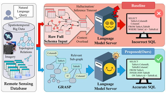
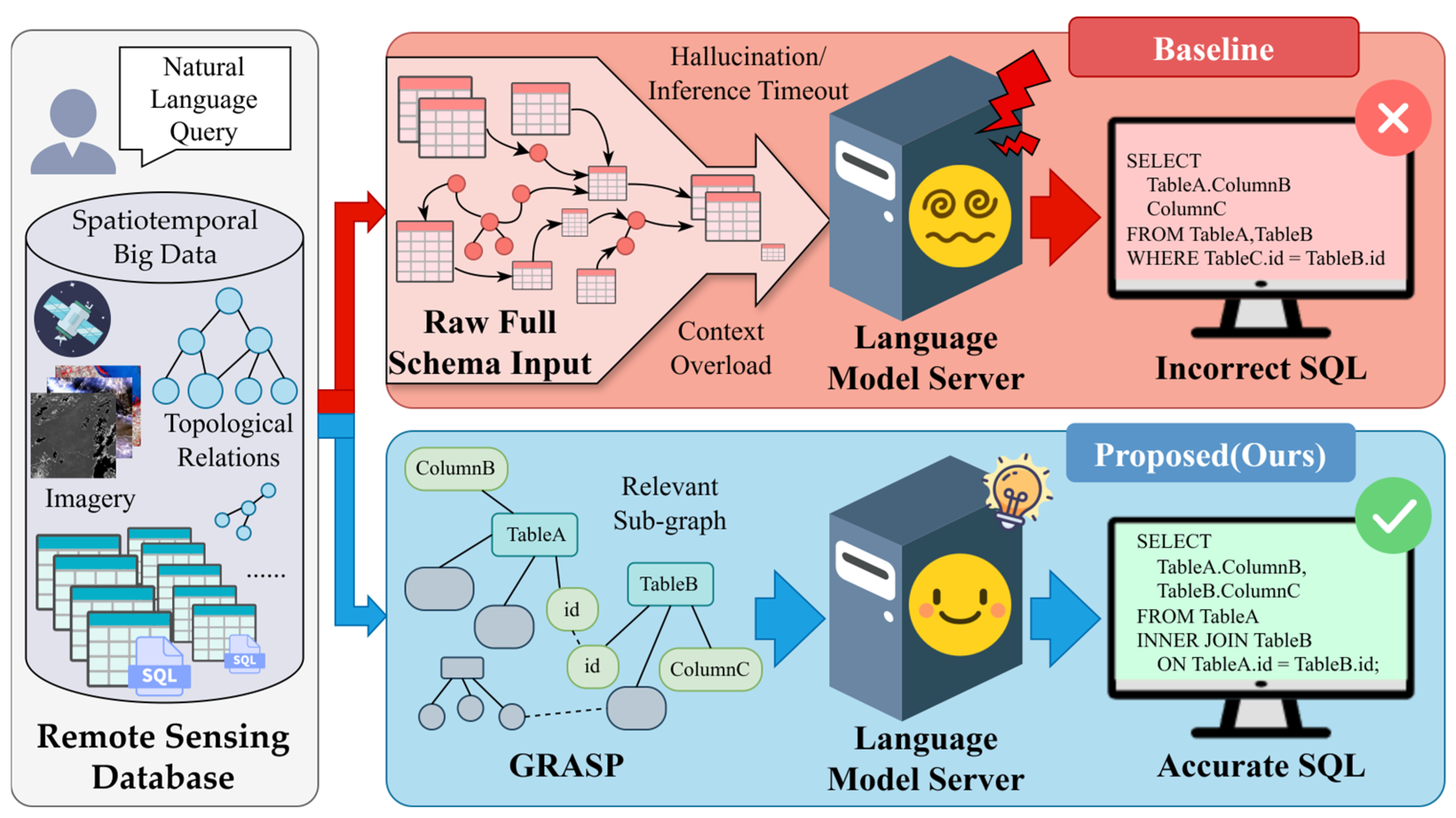
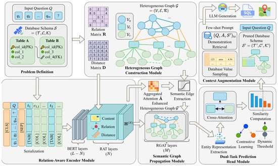
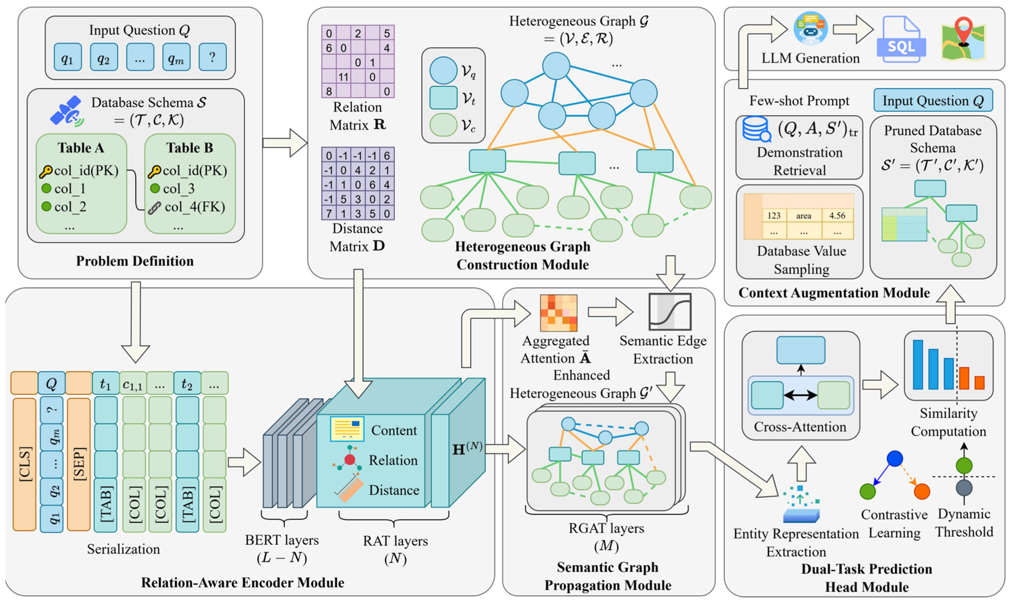
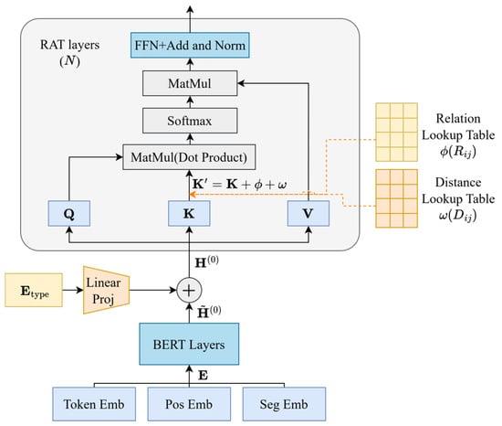
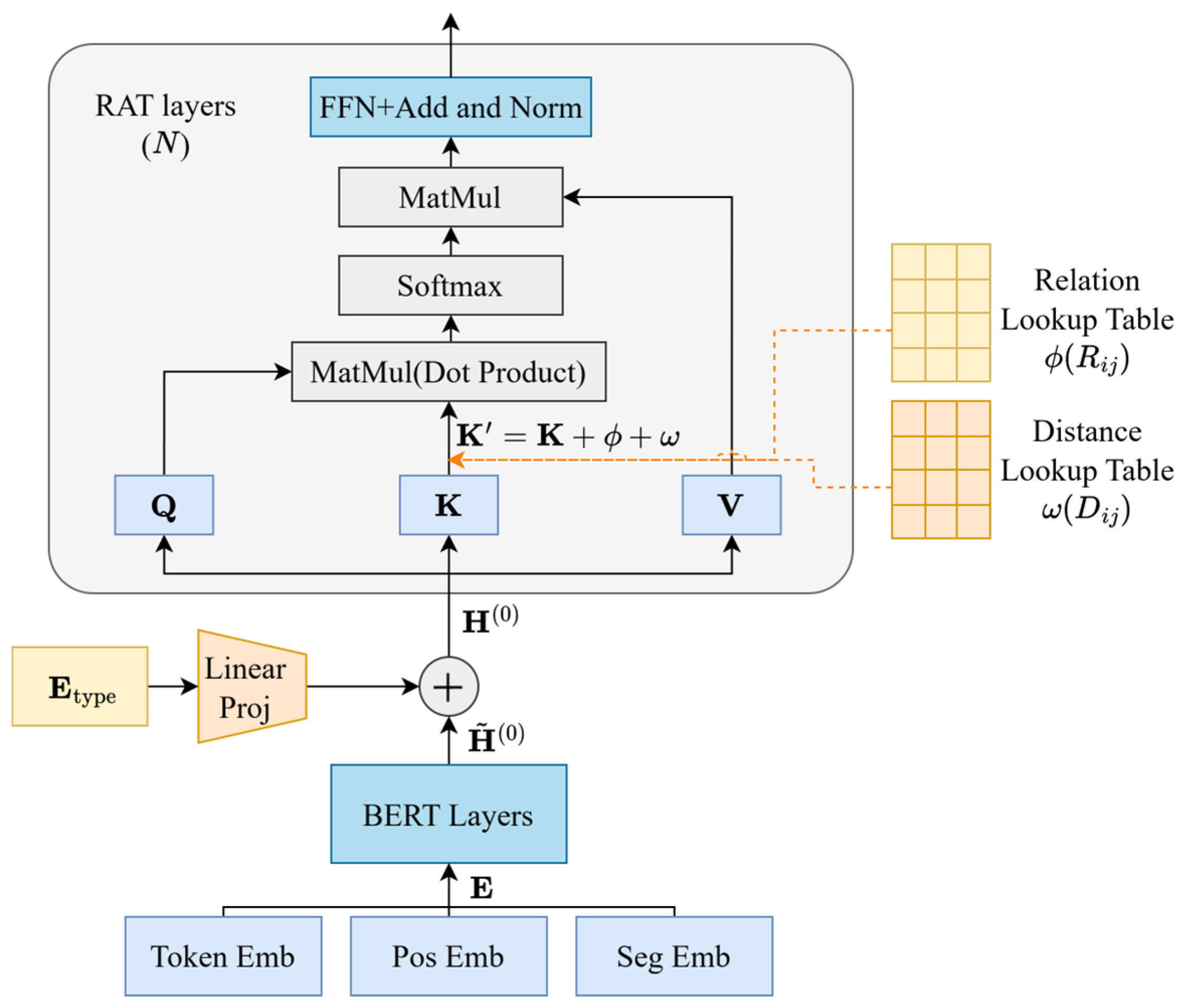
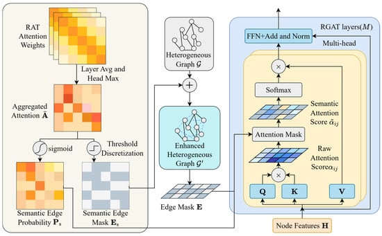
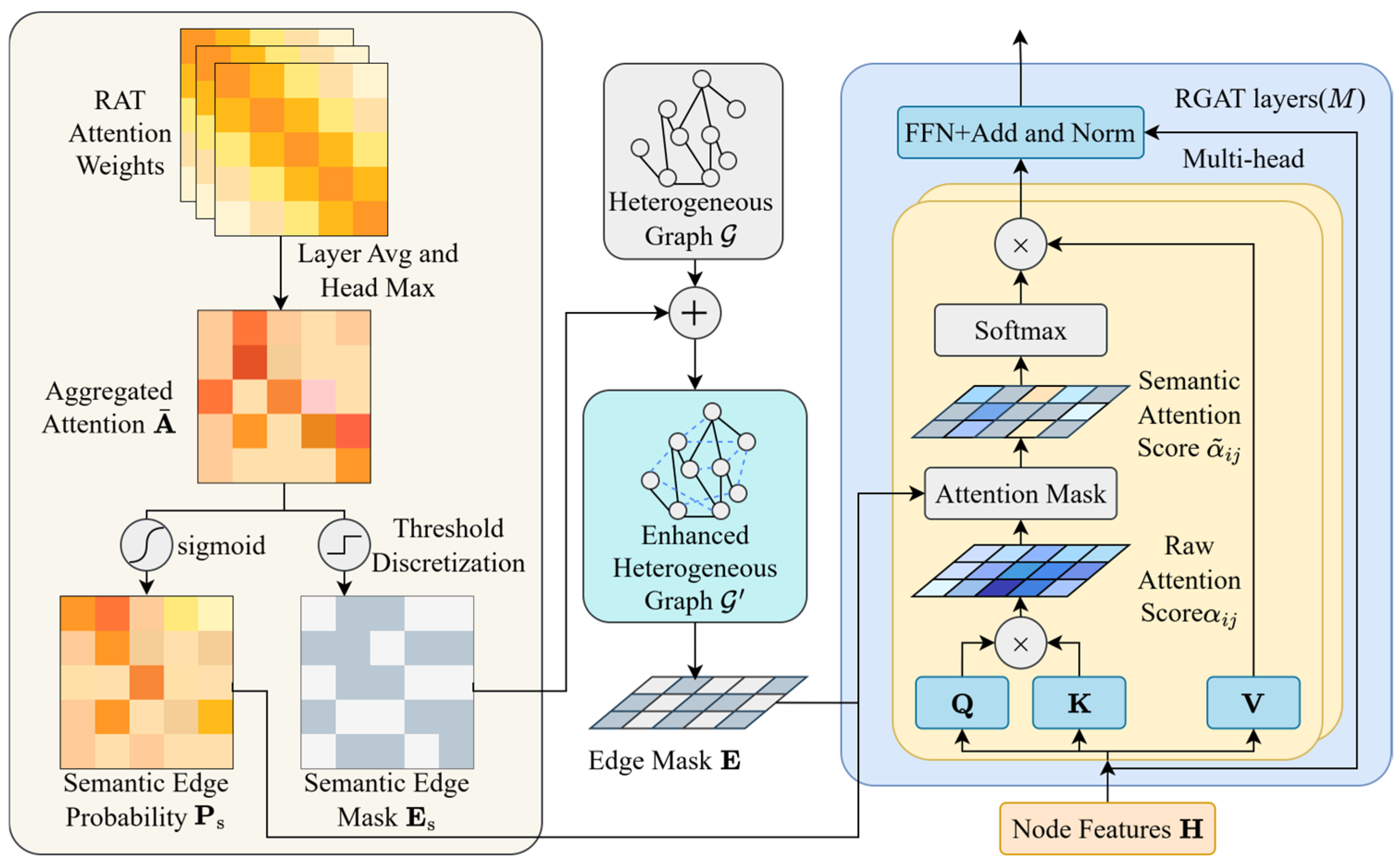
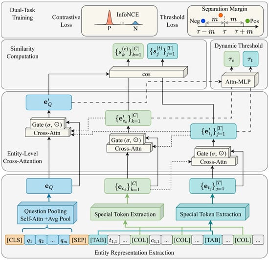
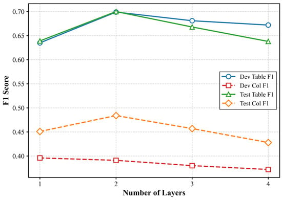
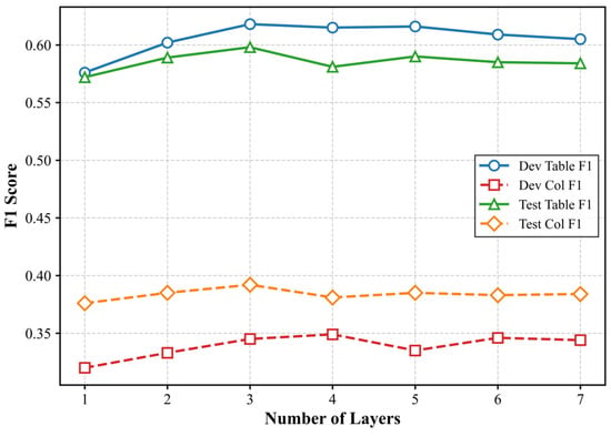
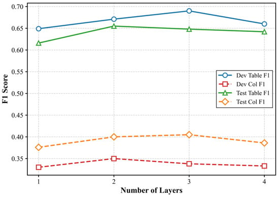
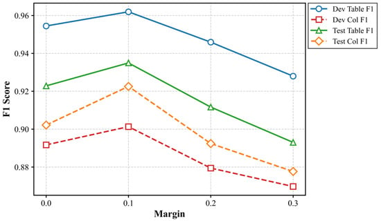
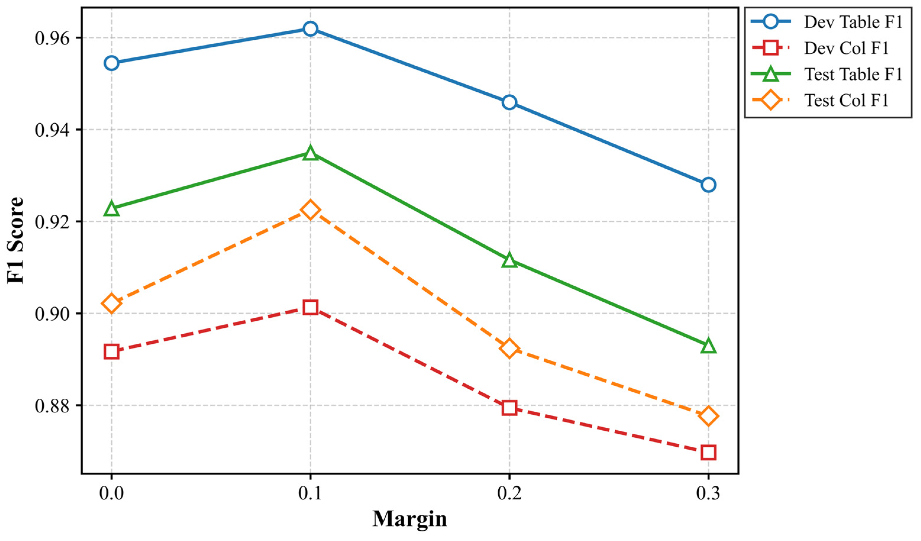
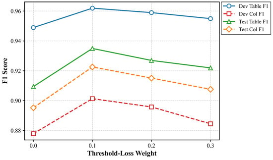
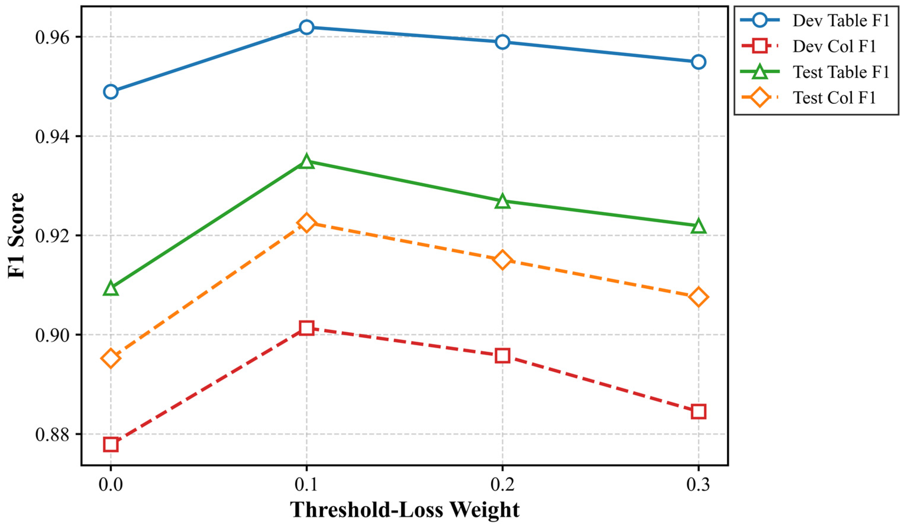
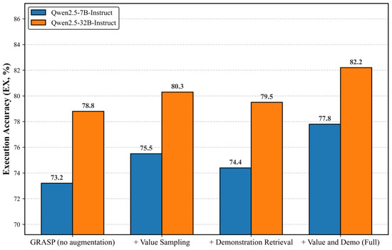
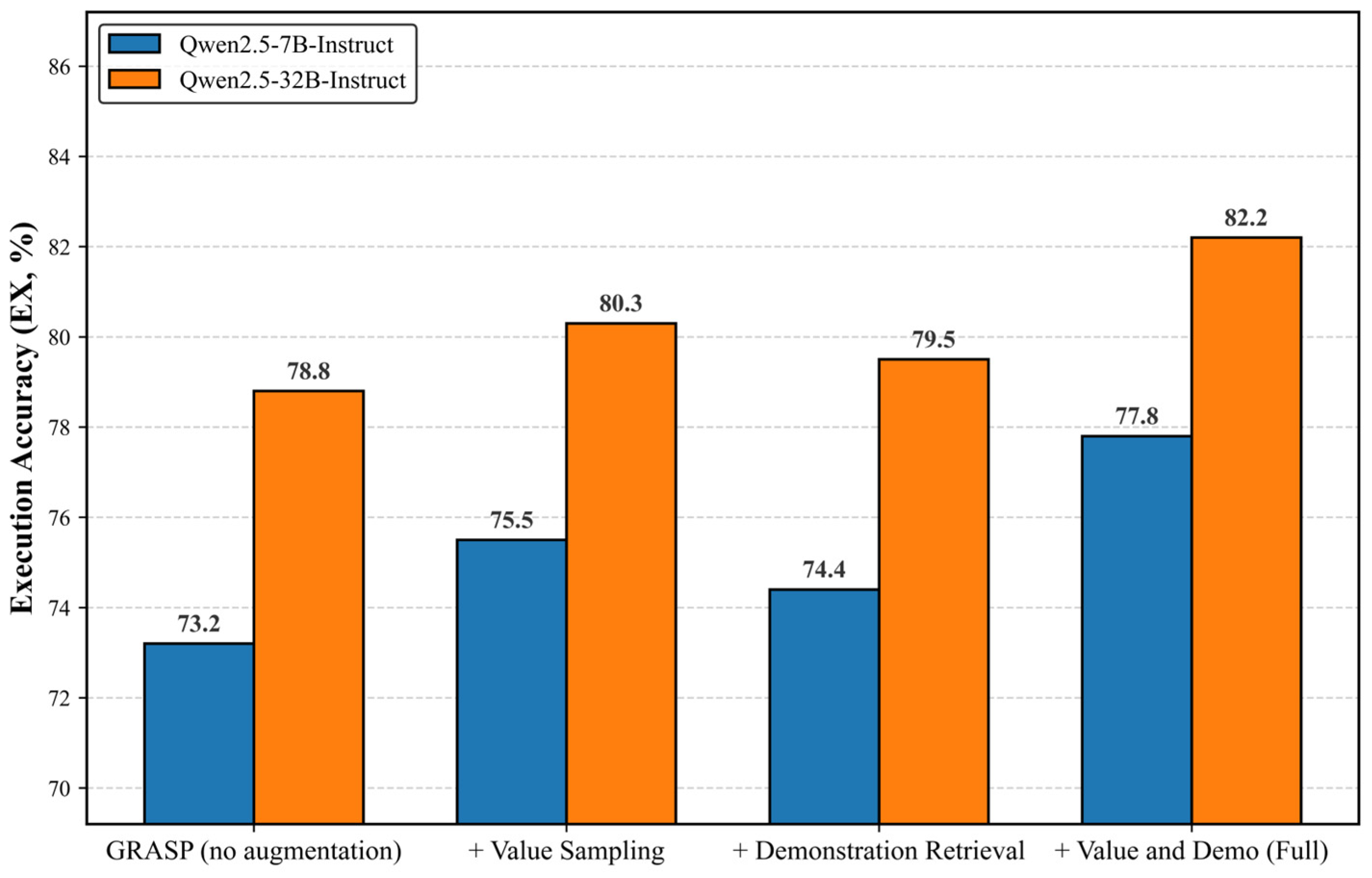
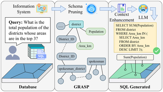
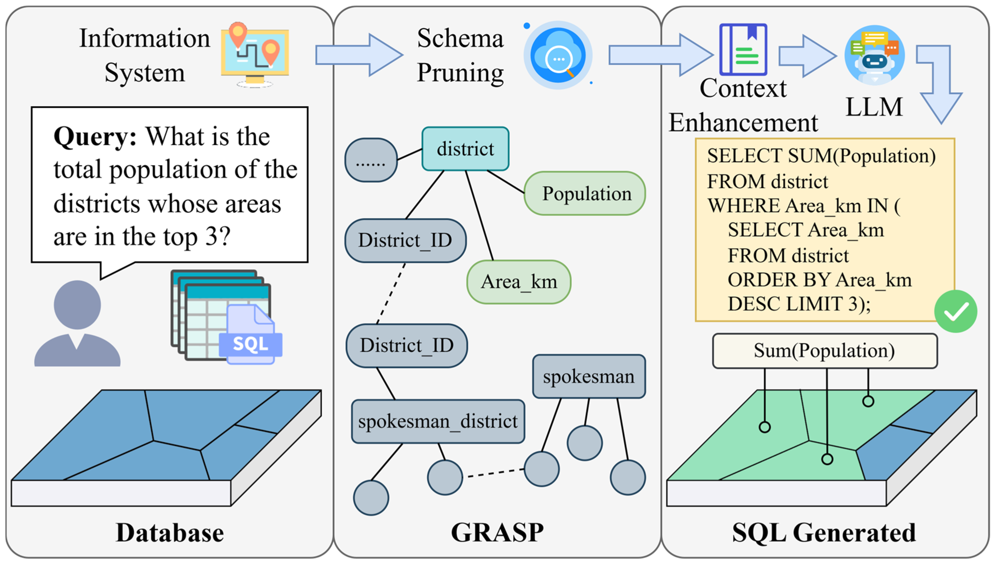
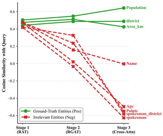
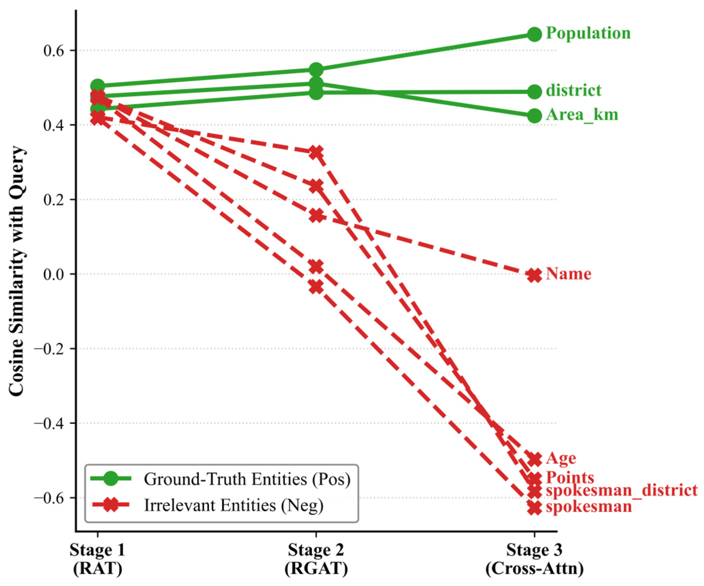
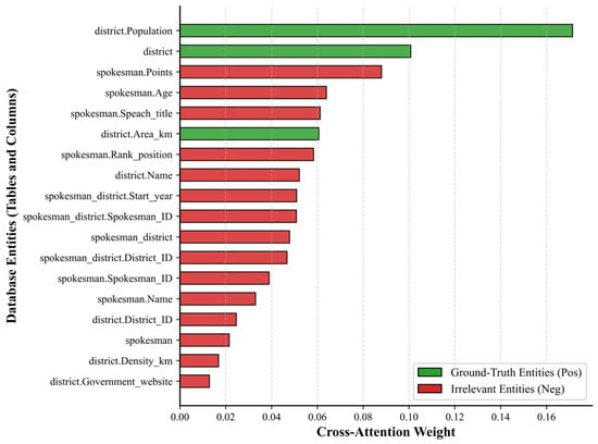
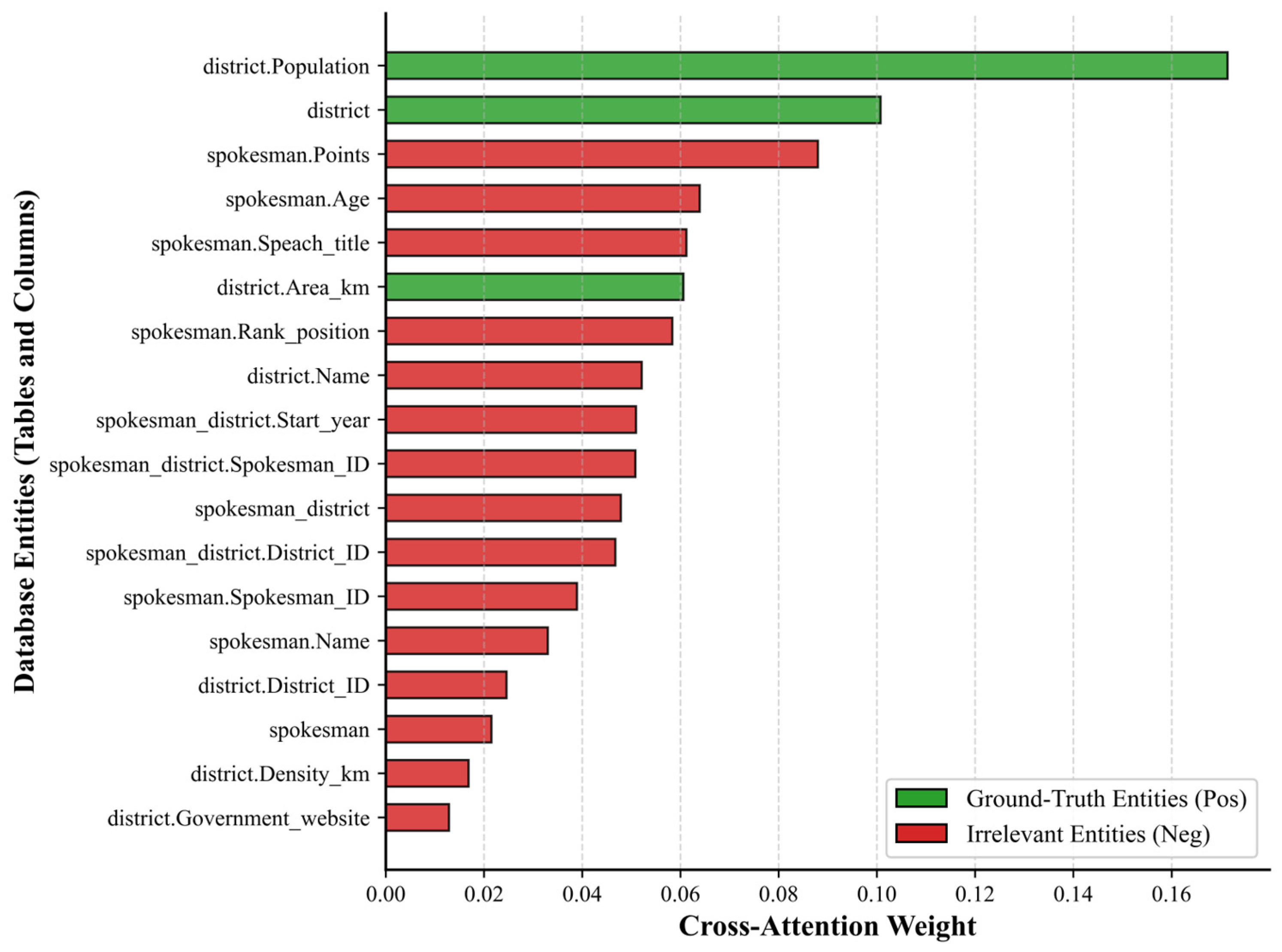
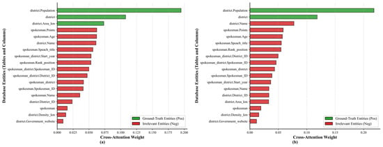
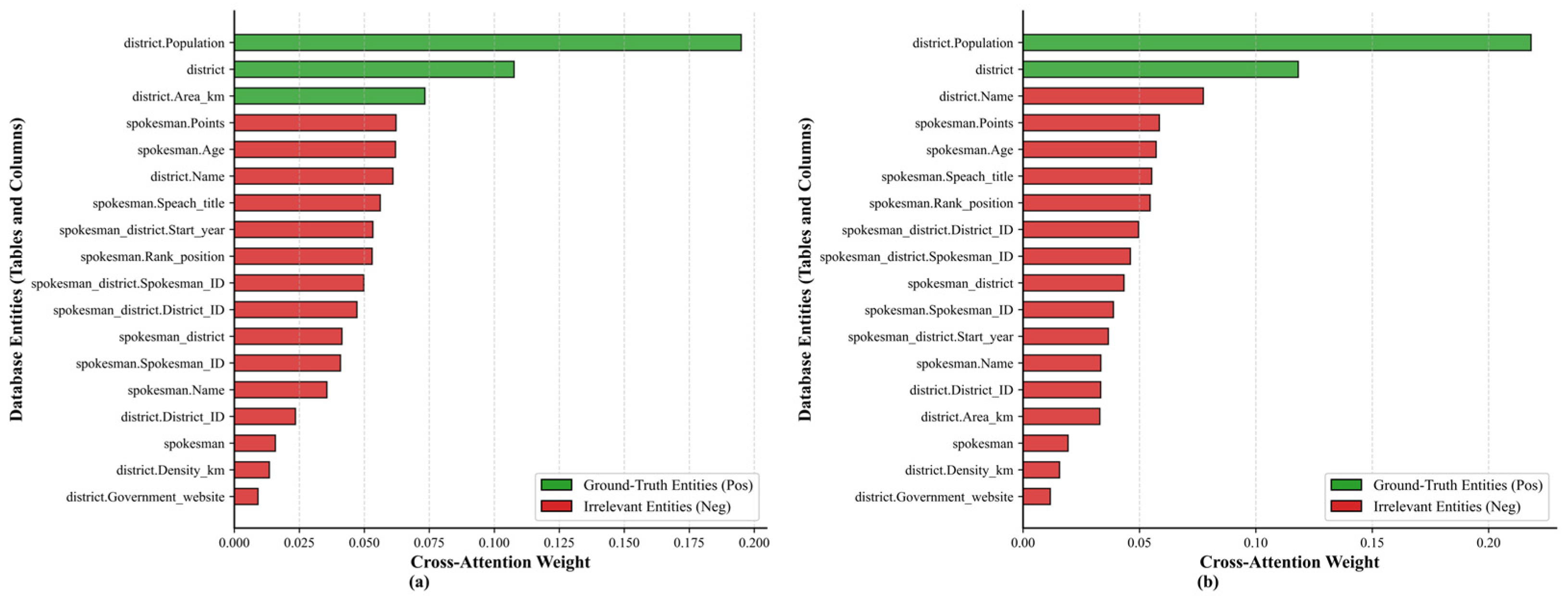
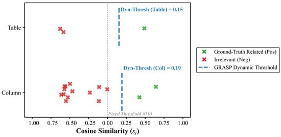
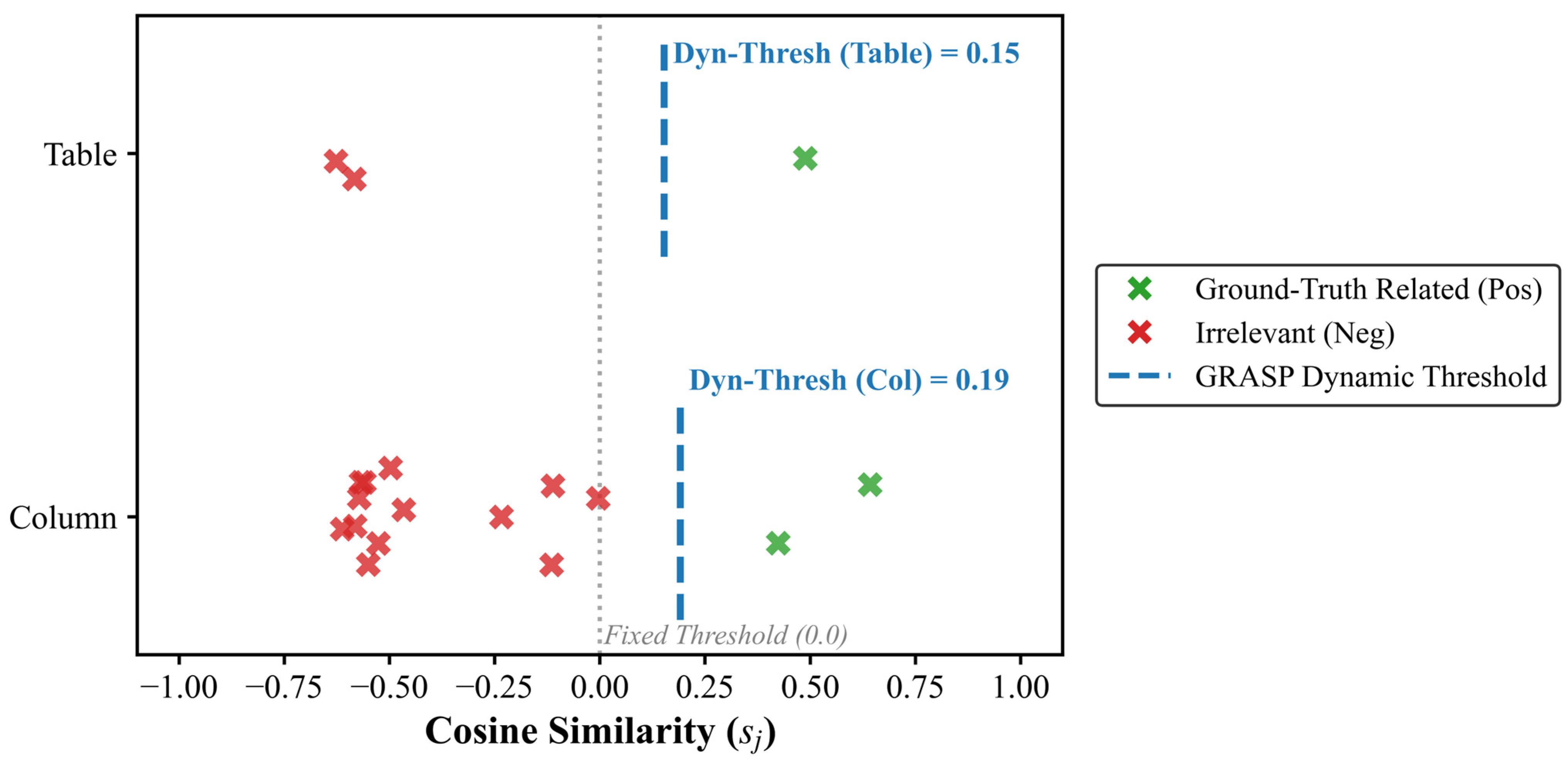

Disclaimer/Publisher’s Note: The statements, opinions and data contained in all publications are solely those of the individual author(s) and contributor(s) and not of MDPI and/or the editor(s). MDPI and/or the editor(s) disclaim responsibility for any injury to people or property resulting from any ideas, methods, instructions or products referred to in the content. |
© 2026 by the authors. Published by MDPI on behalf of the International Society for Photogrammetry and Remote Sensing. Licensee MDPI, Basel, Switzerland. This article is an open access article distributed under the terms and conditions of the Creative Commons Attribution (CC BY) license.