


Abstract
Despite concern over air pollution, fine-scale spatial and demographic disparities in exposure remain largely unquantified in Australian cities due to sparse monitoring and coarse models. In Greater Melbourne, this gap limits neighbourhood-level assessment of PM2.5 exposure and associated environmental inequalities. To address this gap, we integrated 6-month averaged PM2.5 observations (October 2023 to March 2024) from 5 regulatory monitoring stations and 13 low-cost sensors (LCSs) to develop a land use regression (LUR) model estimating concentrations at a 100 m resolution. These estimates were used to calculate population-weighted PM2.5 exposure (PWE) at the mesh block level across Melbourne. To examine factors associated with spatial heterogeneity in PWE, we applied a hybrid modeling framework combining Spatially Explicit Random Forest (Spatial-RF) and Geographically Weighted Regression (GWR), incorporating physical, built-environment, and socio-demographic variables from the Synthesized Multi-Dimensional Environmental Exposure Database (SEED). The Spatial-RF model initially exhibited an R2 of 0.56. After multicollinearity diagnostics using the Variance Inflation Factor (VIF), three key explanatory variables were selected for GWR modeling: the Normalized Difference Vegetation Index (NDVI), the Index of Education and Occupation (IEO), and the proportion of culturally and linguistically diverse populations (CALDP). The developed GWR model achieved higher model performance (R2 = 0.65) than Spatial-RF and global Ordinary Least Squares (OLS) regression (R2 = 0.38), revealing strong spatial non-stationarity. Results show that PWE generally ranged from 5 to 7 µg/m3, exceeding the 2021 WHO air quality guideline, with hotspots in the urban core and along major transport corridors. Elevated exposure occurred in both socioeconomically disadvantaged areas and residents in urban centers with higher socio-economic status, reflecting complex, spatially contingent exposure inequalities. These findings support fine-scale, equity-oriented air quality management.
1. Introduction
Fine particulate matter (PM2.5) is a major urban air pollutant that can penetrate deep into the respiratory system and has been associated with a wide range of adverse health outcomes, posing a severe threat to public health [1,2]. Unlike simple gaseous pollutants, PM2.5 has a complex formation process involving both primary emissions from transport and industrial sectors and secondary aerosols formed through multiphase atmospheric chemical reactions [3]. This complexity results in significant spatial heterogeneity of PM2.5 distribution at intra-urban and neighbourhood-level scales, associated with the interplay between local emission intensity, land-use characteristics, population density, and urban microenvironments [4]. Consequently, accurately characterizing PM2.5 distribution patterns and exposure risks using spatially sparse monitoring networks remains challenging in environmental management and geographic information science [5].
The sparse and uneven spatial distribution of routine monitoring stations has long restricted the accurate characterization of intra-urban air pollution gradients [6,7]. Land Use Regression (LUR) models establish empirical relationships between measurements at stations and geospatial predictor variables, such as traffic intensity, land use characteristics, and population density, thereby addressing the spatial limitations of routine monitoring networks [8,9]. While this approach enables the mapping of the spatial distribution of air pollutants in unmonitored areas, traditional LUR models largely rely on a limited number of regular fixed monitoring stations [10]. This often results in coarse-resolution air pollution mapping that fails to capture fine-scale spatial variations in urban air quality [11]. In recent years, researchers have integrated satellite remote sensing data into the LUR framework to address this issue; however, this approach remains constrained by the coarse spatial resolution of satellite observations and meteorology-induced data gaps, limiting its effectiveness in resolving fine-scale intra-urban pollution patterns [12]. More recently, the increasing use of low-cost sensors (LCSs) in air quality monitoring has provided a practical means to address these limitations [13,14]. The integration of reliability-corrected LCS observations with reference measurements from routine monitoring stations enhances the spatial resolution of air quality monitoring, enabling the detection of fine-scale pollution variability. This data fusion framework provides a robust basis for assessing air quality impacts and examining the joint influence of environmental and socioeconomic factors on neighbourhood-level exposure risks [15,16,17].
However, obtaining high-resolution PM2.5 distribution data is only the first step toward effective pollution control [18]. To develop effective control strategies and reduce public exposure risks, it is crucial to understand population-weighted PM2.5 exposure (PWE) and its associated factors. This is essential for helping governments create more targeted and practical policies [19,20]. Current approaches to identifying the factors associated with air pollution exposure still have several limitations, especially in capturing the combined influence of environmental and socio-economic factors [21,22]. Traditional global modeling approaches, such as Simple Linear Regression (SLR) and Ordinary Least Squares (OLS), operate under the assumption of spatial stationarity [23,24]. These methods presume that the relationships between PWE and its explanatory variables remain constant across the entire study area. This global assumption makes it difficult to capture the complex neighbourhood-level spatial differences and demographic disparities within a city [25]. As an alternative to these global linear models, more recent machine learning (ML) methods perform well in handling non-linear relationships and improving model fit. However, ML models are often criticized as “black boxes” that prioritize predictive performance over interpretability, making it difficult to identify how the significance of factors associated with PM2.5 exposure vary across local areas [26]. To address these issues, combining Spatially Explicit Random Forest (Spatial-RF) with Geographically Weighted Regression (GWR) offers a practical solution. The Spatial-RF model allows us to rank and select variables based on their importance, effectively identifying the key explanatory variables of PM2.5 exposure [27]. The GWR model then addresses the limitations of global regression by capturing how the influence of these explanatory variables changes across different locations [28]. Combining these two methods can provide a systematic framework for identifying how different factors are associated with PWE at the neighbourhood-level.
In this study, we developed an integrated, neighbourhood-level framework to quantify and interpret spatial heterogeneity and demographic disparities in PWE across Melbourne. First, we combined regulatory monitoring data with a dense network of LCSs to develop a high-resolution LUR model, estimating PM2.5 concentrations at 100 m resolution across Melbourne. Second, we estimated mesh-block-level PWE based on previous PM2.5 modeling results and evaluated air pollution exposure inequality across economic and educational-occupational dimensions. Finally, we applied a hybrid modeling framework combining Spatial-RF and GWR, incorporating physical, built-environment, and socio-demographic variables from the Synthesized Multi-Dimensional Environmental Exposure Database (SEED), to identify key explanatory variables of spatial heterogeneity in PWE at the neighbourhood-level. Neighbourhood-level exposure assessment enables the identification of fine-scale spatial disparities and exposure inequities that are not captured by aggregate analyses. The integrated approach developed in this study moves beyond reliance on sparse regulatory monitoring and single modeling strategies by systematically combining multi-source observations with a hybrid Spatial-RF–GWR framework. Unlike previous studies that have emphasized either predictive accuracy or spatial interpretability, this framework achieves both high-resolution exposure estimation at a 100 m scale and the spatially explicit identification of associated factors at the neighbourhood level. The explicit integration of fine-scale exposure modeling with inequality assessment and spatial heterogeneity analysis extends conventional concentration mapping toward a more comprehensive, equity-oriented perspective for urban air quality management.
2. Materials and Methods
2.1. Study Area
Melbourne is the capital of Victoria, Australia, and the country’s largest city. This study focuses on the entire Melbourne metropolitan area (Figure 1), which is geographically located between approximately 37°45′–38°20′ S latitude and 144°35′–145°50′ E longitude, covering a total area of about 10,000 km2 [29]. The study area encompasses the full urban gradient, from the central business district (CBD) and high-density inner-city areas to low-density outer suburbs, allowing for a comprehensive representation of air pollution characteristics under different land-use types and levels of human activity. Geographically, Melbourne is situated around Port Phillip Bay, bordered by the Victorian Volcanic Plain to the west and the Dandenong Ranges to the east, with the Yarra River flowing through the city center. The overall topography is relatively flat, which, under typical meteorological conditions, facilitates the dispersion and dilution of pollutants.
Figure 1.
Study area and spatial distribution of monitoring stations in metropolitan Melbourne, Australia. The red circles represent the regulatory EPA stations, while the green circles denote the locations of LCSs.
As one of Australia’s fastest-growing cities, Melbourne has seen rapid urbanization over the past few decades. This growth has led to higher PM2.5 emissions from human activities, with road traffic identified by Environment Protection Authority (EPA) Victoria as the primary pollution source. To accurately capture these pollution patterns, this study utilizes a monitoring network of 18 stations distributed across the metropolitan area (Figure 1). This network integrates regulatory EPA stations (marked as red circles) with LCSs (shown as green circles) to better represent both high-traffic regions and residential zones. Integrating these multi-source observations and high-resolution population data enabled us to develop an LUR model for mapping PM2.5 at a fine scale. This approach allows for a detailed estimation of neighbourhood-level exposure, providing a practical basis for local air quality management and environmental health assessments.
2.2. Data Collection and Processing
This study used six months of continuous PM2.5 observations (October 2023 to March 2024) from 18 monitoring stations across the Melbourne metropolitan area (Figure 1), providing a reliable data foundation for developing a city-scale LUR model. These include five regular fixed monitoring stations operated by the EPA Victoria and 13 LCSs from the PurpleAir platform. A rigorous three-step workflow was applied to the hourly PM2.5 concentrations from 13 LCSs, ensuring data integrity and addressing potential sensor biases. First, the raw measurements were adjusted using the US EPA-recommended correction equation implemented on the PurpleAir platform [30]. This framework addresses hygroscopic growth and optical artifacts by incorporating relative humidity (RH) as a key covariate, thereby aligning the sensor response with reference-grade monitoring standards. Second, a robust anomaly detection procedure was implemented using the median absolute deviation (MAD) method. Observations at each station exceeding the threshold of |x − median(x)| > 3 × MAD were removed, minimizing the influence of extreme values and skewed distributions commonly found in high-resolution air pollution datasets. Finally, a temporal scaling correction was introduced to seamlessly align the LCS measurements with the regulatory monitoring network. Specifically, the scaling factor was computed as the ratio between the mean PM2.5 concentration measured at the five EPA regulatory stations and the mean concentration across all LCS sites over the six-month study period. This scaling factor was then applied multiplicatively to every hourly record across all LCS stations. This integrated calibration framework improves consistency between heterogeneous data sources, effectively minimizing bias propagation and providing a reliable basis for the subsequent LUR modeling.
The monitoring stations, which are widely deployed throughout the Melbourne metropolitan area to cover key geographical and functional units, are densely clustered in the CBD and core urban zones. This configuration, which closely matches the spatial extent of traffic-intensive areas, allows for robust characterization of local pollution features and concentration gradients. Additionally, some sites are distributed in low-density suburbs and adjacent nature reserves to provide complementary spatial coverage. Overall, the monitoring network provides continuous spatial coverage from the urban core to the outer suburbs, enabling a systematic representation of PM2.5 spatial variability and the urban gradient in Melbourne, and establishing a solid data foundation for subsequent model development.
Figure 2 illustrates the multi-source geospatial datasets used in this study, showcasing both metropolitan-wide patterns and localized urban details. Figure 2a,f show the broad spatial distribution of land use types and Normalized Difference Vegetation Index (NDVI) across the entire Melbourne metropolitan area, representing the regional environmental and vegetation context. To provide a clearer view of the high-resolution data, Figure 2b–e focus on a representative area within the urban core. These panels detail the population distribution (Figure 2b), building footprints (Figure 2c), bus stops (Figure 2d), and the main road network (Figure 2e). For these localized views, small inset maps are included to show the specific location of the study area within the broader city. All geospatial data were integrated into a unified coordinate system and organized within a GIS database, providing a consistent foundation for developing the LUR model and assessing population.
Figure 2.
Potential predictor variables in the LUR model for the Melbourne study area. The figure consists of six panels: (a) land use data; (b) population data; (c) building footprint data; (d) bus stop locations; (e) main road network; and (f) NDVI.
The spatial resolution and data sources are summarized in Table 1. Land use data were obtained from OpenStreetMap (OSM) and reclassified based on the CORINE land cover classification scheme following the European ESCAPE project, aggregating surface cover types within the study area into five major categories: high-density residential areas, low-density residential areas, industrial areas, urban green spaces, and natural areas (Figure 2b).
Table 1.
Resolution and Data Sources of GIS Datasets.
Road network data were obtained from OSM. All roads in the database were classified as motorway, motorway_link, trunk, trunk_link, primary, primary_link, secondary, secondary_link, tertiary, tertiary_link, residential, service, living_street, track, and various non-vehicular paths (e.g., footway, cycleway). Among these, motorway, trunk, primary, secondary, and tertiary (including their respective link roads) were regrouped as main roads (Figure 2e). Traffic volume data, including total traffic counts and heavy-duty vehicle volumes, were acquired from the Department of Transport and Planning. A Python-based data processing script was developed to spatially link traffic volume information to the road network. For road segments lacking direct traffic measurements, a location-based spatial interpolation approach was applied, whereby traffic volumes were estimated using data from nearby road segments. This procedure resulted in a comprehensive traffic volume dataset covering all roads within the study area.
Bus stop data were obtained from OSM and include point-based records of bus stops across the entire Melbourne metropolitan area (Figure 2d). This dataset provides precise spatial locations for each bus stop.
Population and household data were obtained from the smallest statistical units (mesh blocks) released in the 2021 Australian Census. To facilitate spatial analysis, the polygon-based vector data containing population and household counts were converted into point features, with each point located at the geometric centroid of the corresponding mesh block. All attribute information was retained, resulting in a high-precision population distribution dataset (Figure 2b).
Building data were obtained from the Global Building Atlas dataset, which provides detailed vector footprints and height attributes for buildings across the entire Melbourne metropolitan area. The dataset is organized at the individual building level and includes building polygon boundaries together with their corresponding height values, offering a high-precision representation of the built environment to support urban morphology analysis and pollutant dispersion modeling (Figure 2c).
2.3. Potential Predictor Variables
This study employed PyLUR 1.0.0, an efficient LUR modeling framework utilizing Python 2.7 and the GDAL/OGR libraries, to generate potential predictor variables [31]. PyLUR integrates functions for buffer generation, proximity analysis, and meteorological data integration, enabling automated processing of the variable generation workflow.
The PyLUR software automatically performed buffer analysis centered on each monitoring station, using radii of 1000, 500, 300, 200, and 100 m. For some variables, finer-scale buffers of 50, 25, and 10 m were also included to capture detailed built environment features. Based on these buffers, the following variables were calculated:
- Population variables: Using mesh block census data, the total population and number of households within each buffer were computed.
- Road traffic intensity variables: Based on road network data, the total road length within each buffer was calculated. To represent the overall emission source intensity, traffic volume data were integrated to calculate traffic load variables, specifically utilizing bidirectional (total two-way) average daily traffic and heavy-duty vehicle volumes.
- Land use composition: Using the reclassified Corine land cover system, the area proportions of different land use types within each buffer were calculated.
- Urban form: Based on Global Building Atlas data, variables such as building footprint area, building height, and building density were extracted.
Proximity variables were created by calculating the shortest distance from each monitoring site to the nearest main road and bus stop. Meteorological variables were integrated using parameters obtained from the ERA5 reanalysis dataset for the study period from October 2023 to March 2024. These included six-month mean values of the 10 m zonal and meridional wind components (u10, v10), 2 m dew point temperature (d2m), 2 m air temperature (t2m), surface pressure (sp), and boundary layer height (blh), which were used to characterize regional atmospheric dispersion conditions. Meteorological variables were derived by extracting data from monthly ERA5 NetCDF files at each station’s coordinates and calculating the six-month average for each site.
A total of 160 potential predictor variables were considered in the modeling (Table 2). These variables differ in coding schemes, units, buffer sizes, and assumed directions of effect, and collectively represent factors related to land use, building configuration, road networks, and background geographic characteristics. Together, they comprehensively captured multiple environmental factors associated with the spatial variability of PM2.5 concentrations, including traffic emissions, urban form, population activity, and atmospheric dispersion conditions. This extensive variable set provided a robust foundation for subsequent feature selection and model development.
Table 2.
Potential predictor variables considered in model building, along with their variable codes, units, buffer sizes, and directions of effect.
2.4. LUR Model Development and Validation
As shown in Figure 3, this study developed a LUR framework to construct the mathematical relationship between observations (six-month averaged PM2.5 concentrations) and potential predictor variables across the Melbourne metropolitan area. The modeling process was standardized and executed using PyLUR 1.0.0, a robust open-source tool developed by our research group for high-efficiency spatial modeling. Its capability to accurately characterize the spatial distribution of air pollutants has been validated in previous high-impact studies.
Figure 3.
Flowchart of LUR model development and verification.
2.4.1. Variable Selection and LUR Model Development
Following the recommendations of the ESCAPE project, the LUR model was developed using a five-step supervised forward stepwise procedure [32]. First, each potential predictor variable was individually regressed against the PM2.5 concentrations measured at monitoring sites using univariate regression. The variable with the highest adjusted R2 was then selected as the starting predictor variable in the LUR model. An initial model was constructed only when the regression coefficient of this variable was consistent with the predefined direction of effect listed in Table 2. Second, each remaining potential predictor variable was added individually to the model obtained in step 1, and the adjusted R2 of the resulting model was recorded. This process was repeated for all other remaining variables, with the adjusted R2 values recorded separately. Third, among all the results from step 2, the remaining variable that led to the largest increase in adjusted R2 was considered for inclusion in the model, provided it satisfied three conditions: the increase in adjusted R2 exceeded 1%; the coefficient of the new variable aligned with its predefined direction of effect as listed in Table 2; and the signs of the coefficients for the existing variables remained unchanged between the previous and current models. Fourth, steps 2 and 3 were repeated until no remaining potential predictor variable could improve the adjusted R2 of the previous model by more than 1%. Finally, any predictor variables that were not statistically significant (p-value > 0.1) were removed from the model one at a time, starting with the largest p-value, until all variables in the final model were statistically significant.
Following the construction of the final LUR model, we assessed model diagnostics to ensure robustness. Influential observations were evaluated using Cook’s Distance. Multicollinearity among predictors was examined using the VIF, and variables with high VIF values were removed to mitigate multicollinearity. Residual spatial autocorrelation was evaluated using the Global Moran’s I to check whether model residuals exhibited any spatial clustering. These procedures ensure that the model structure is sound and suitable for spatial analysis.
2.4.2. Model Validation
To evaluate the predictive performance of the model, Leave-One-Out Cross-Validation (LOOCV) and five-fold cross-validation were employed, with the R2 and Root Mean Square Error (RMSE) serving as the primary evaluation metrics. In the LOOCV process, each monitoring station was sequentially used as an independent test set, while the remaining 17 stations form the training set to reconstruct the LUR model. This process was iterated 18 times (18 being the total number of monitoring stations) to ultimately obtain predicted concentrations for all sites. In the five-fold cross-validation, all stations were randomly partitioned into 5 equal-sized groups. Each group was used as a test set alternatively, while the remaining 4 groups were combined into a training set for modeling; this process was repeated 5 times to ensure that every group was fully validated.
The final model is expressed in the following general form:
In this equation, PM2.5 represents the predicted particulate matter concentration, β0 is the intercept, βi denotes the regression coefficient for each predictor variable Xi, and ε is the error term. The variables included in the model typically comprise population density, road length, proportions of different land use types, green space coverage, and meteorological factors, reflecting the combined influence of human activities and environmental features on the spatial distribution of PM2.5.
2.5. Spatial Mapping Across the Entire Study Area
Although the LUR modeling approach is relatively straightforward, its application for urban-scale air pollution mapping, particularly when high-resolution input and output data are required (100 m resolution), often entails substantial computational costs [33,34,35]. Due to limitations in computing resources and data processing capacity, many previous studies have typically reported only the model equations or produced low-resolution pollution maps.
To overcome this limitation, the study employed the PyLUR software, which was developed by others based on the GDAL/OGR library for LUR modeling and pollution mapping. Together with the finalized LUR model, it was used to generate a 100 m resolution spatial map of PM2.5 across the Melbourne metropolitan area. The procedure consisted of the following steps: first, a 100 m × 100 m regular grid covering the entire study area was established; next, the PyLUR package was run to extract and compute relevant land use and environmental variables within each grid cell; finally, PM2.5 concentrations were estimated for each cell based on the LUR model equation. The resulting predictions were imported into ArcGIS 10.8 for visualization, producing the final spatial maps.
2.6. Neighbourhood-Level PWE Assessment and Multi-Dimensional Correlate Analysis Framework
To systematically assess fine-scale spatial patterns of PWE in the Melbourne metropolitan area and identify the factors associated with these variations, this study developed a three-step quantitative framework, progressing from pollution concentration pattern analysis to population exposure assessment and finally to spatial correlate analysis (Figure 4).
Figure 4.
Technical framework for neighbourhood-level PWE assessment and correlate analysis. Getis-Ord Gi* is a local spatial statistic used in the ArcGIS hot spot analysis to identify statistically significant hot spots and cold spots. SA1 (Statistical Area Level 1) and SA3 (Statistical Area Level 3) are statistical units defined by the Australian Statistical Geography Standard (ASGS). SEED provides integrated, high-resolution environmental and socioeconomic indicators for neighbourhood-level exposure and correlate analysis.
First, to identify the spatial clustering characteristics of PM2.5 concentrations, this study applied the Getis-Ord Gi* Hot Spot analysis to point vector data representing PM2.5 concentrations at a 100 m resolution. Spatial adjacency was defined using a distance threshold. The analysis aimed to detect statistically significant clusters of high concentrations (hot spots) and low concentrations (cold spots), thereby revealing the intrinsic spatial structure of PM2.5.
Building on the established spatial distribution patterns of PM2.5 concentrations, the study further assessed the actual exposure risk to residents. Point-based concentration data were first converted into 100 m resolution raster layers and then overlaid with mesh- block-level population data provided by the ABS. Using a PWE metric, PWE levels were quantified at the mesh-block-level, thereby characterizing residents’ actual exposure. This metric was calculated using Equation (2) [36], integrating both pollution concentrations and population distribution to reflect their spatial co-occurrence effect.
Here, PMi represents the PM2.5 concentration in the i-th grid cell, and POPi denotes the population within the same cell. Through spatial aggregation, PWE values were obtained at the mesh-block-level, which were then used to generate spatial distribution maps. Furthermore, SA1 units were grouped based on the Index of Economic Resources (IER) and the Index of Education and Occupation (IEO) to quantitatively assess the socio-economic disparities in exposure levels.
To elucidate the multi-dimensional factors underlying the observed spatial patterns, this study developed a hybrid modeling framework combining Spatial-RF and GWR. The specific procedure was as follows:
- Spatially informed variable selection: SA1-level PWE was treated as the dependent variable. A Spatial-RF model was constructed by incorporating both explanatory variables and spatial coordinates (centroid x and y) to account for spatial context. To reduce spatial overfitting, a spatial block cross-validation scheme (5-fold GroupKFold) was implemented, in which spatial units were grouped by grid-based blocks. Model performance was evaluated using spatial cross-validated R2. After fitting the Spatial-RF model on the full dataset, variable importance rankings were extracted, and the most influential non-spatial variables were retained for subsequent analysis.
- Multicollinearity diagnosis: The selected variables were standardized and evaluated using the VIF. Variables with VIF values exceeding 3 were iteratively removed until all remaining predictors satisfied the criterion of VIF < 3. This conservative threshold was adopted to minimize multicollinearity and ensure a stable and parsimonious set of explanatory variables. The procedure enhanced the robustness and interpretability of the subsequent regression models.
- Global and local regression modeling: A global OLS model was first fitted using the optimized variable set to provide a baseline estimate of spatially constant relationships. Subsequently, a GWR model with an adaptive bandwidth and bisquare kernel was con-structed. Unlike global regression, GWR allows regression coefficients to vary across space, thereby capturing spatial non-stationarity in the strength and direction of associations between explanatory variables and PWE.
The explanatory variables for PWE modeling were selected from the SEED and organized into four thematic domains. Physical environmental variables included Land Surface Temperature (LST), Excess Heat Factor (EHF), NDVI, and Canopy Height (CH). Built-environment characteristics were represented by the Normalized Difference Built-up Index (NDBI), Street Connectivity (SC), Land Use Diversity (LUD), Distance to Public Transit (DPT), and Sky View Factor (SVF) or Green View Factor (GVF). Atmospheric conditions were captured via Nitrogen Dioxide (NO2) and Aerosol Optical Depth (AOD). Socio-economic conditions were described using the IER, the IEO, and the proportion of culturally and linguistically diverse populations (CALDP). To prevent overfitting and enhance model interpretability, variables that did not directly represent emission sources, atmospheric processes, or dispersion conditions were excluded. Specifically, health outcomes and perceptual indicators were removed prior to the modeling process. A Spatial-RF model was first applied to screen key PWE explanatory variables from the environmental, built, and socio-economic domains, and only variables with high importance and low redundancy were subsequently incorporated into the GWR analysis. All variables were aggregated to the SA1 spatial unit.
This framework enables systematic analysis of fine-scale PWE patterns in Melbourne, their socio-economic disparities, and the spatially heterogeneous factors shaping these patterns, through an integrated approach of pattern detection, exposure assessment, and spatial correlate analysis.
3. Results
3.1. Spatial Distribution Characteristics of PM2.5 Concentration
The predictor variables selected in the final LUR model were POP_200 (population within a 200 m buffer) and ROADLENGTH_200 (road length within a 200 m buffer). Overall, the model demonstrated a robust fit, accounting for 62% of the spatial variance in PM2.5 concentrations (R2 = 0.62). Model performance was validated using data from the 18 monitoring stations, with site-specific residuals and percentage biases detailed in Table 3. Statistical assessment yielded a Mean Absolute Error (MAE) of 0.63 µg/m3, a RMSE of 0.84 µg/m3, and a Mean Absolute Percentage Error (MAPE) of 9.1%. The Global Moran’s I test confirmed the absence of significant spatial autocorrelation in the model residuals (I = 0.040, p = 0.113). This result indicates that the LUR model effectively captured the spatial structure of PM2.5 concentrations, leaving the remaining errors randomly distributed across the study area. Collectively, these metrics confirm that the model provides reliable and acceptable estimates for fine-scale air quality assessment.
Table 3.
Comparison between observed and predicted PM2.5 concentrations, residuals, and percentage bias across 18 monitoring stations (units: µg/m3 for concentrations and residuals).
To further evaluate the predictive performance and robustness of the model, we conducted LOOCV and five-fold cross-validation. LOOCV yielded an R2 of 0.55 and an RMSE of 0.61 µg/m3. Five-fold cross-validation produced an average R2 of 0.72 and an average RMSE of 0.57 µg/m3 (SD = 0.03). The observed discrepancy between these metrics was primarily linked to the limited number of monitoring stations (n = 18). In such a small-sample context, LOOCV was inherently sensitive to individual sites or local outliers, whereas five-fold cross-validation results can fluctuate based on how the data were randomly partitioned. Despite these numerical variations, both validation metrics remain within an acceptable range for high-resolution LUR modeling.
Based on the combined model fitting and validation results, the final form of the LUR model was determined as follows:
The model yields positive regression coefficients for all variables, indicating that higher population density and denser road networks are associated with elevated local PM2.5 concentrations. This is consistent with typical urban emission patterns.
The 100 m resolution PM2.5 spatial predictions (Figure 5) illustrate the distribution patterns across the Melbourne metropolitan area. A clear urban-to-rural gradient is observed, with higher concentrations in the city center and lower levels toward the suburbs. High-concentration zones are primarily found in the CBD and surrounding high-density built-up areas, such as Southbank, Carlton, West Melbourne, and Docklands. These areas are characterized by intense human activity and dense road networks, which is consistent with the predictor variables identified by the model.
Figure 5.
PM2.5 spatial distribution in the Melbourne metropolitan area based on the LUR model (100 m resolution).
While these high-resolution maps provide valuable insights into pollution hotspots, it is important to avoid overstating the spatial precision of the exposure surfaces. Given the inherent uncertainties in spatial modeling and their propagation into PWE estimates, our findings are designed to represent robust regional pollution trends rather than absolute individual-level exposures.
In contrast, the outer urban areas, particularly those with higher green cover or semi-rural characteristics, such as Emerald, Monbulk, Romsey, and Panton Hill, generally exhibit lower PM2.5 concentrations. These areas typically have fewer potential emission sources and lower traffic density, while the relatively high vegetation cover may contribute to pollution mitigation, resulting in pollutant levels significantly lower than those observed in the urban core.
To evaluate the fine-scale spatial heterogeneity of air quality across the metropolitan area, two representative transects (A and B) were extracted for detailed profile analysis (Figure 6). Transect A is an 8 km south-to-north profile that begins at the Port Phillip Bay coastline and bisects the primary pollution hotspot in the Melbourne CBD. The concentration remains at a baseline level for the first 1.5 km and then escalates sharply, reaching a maximum of approximately 10.2 µg/m3 at the 2.1 km mark. This peak aligns with the high-density commercial core of the city. Beyond this peak, the concentration exhibits a fluctuating decline as the transect moves through the northern inner-city suburbs. In contrast, Transect B provides a 10 km west-to-east cross-section of Greater Dandenong, a significant industrial and residential hub in the southeast. This profile maintains a relatively stable level initially, but transitions into a distinct multi-peak distribution between 4 km and 8 km, reflecting the complex spatial interplay between local industrial emissions and dense residential zones in this secondary hotspot. Together, these profiles characterize the typical urban-to-peripheral gradients and the influence of land-use intensity on localized PM2.5 distributions.
Figure 6.
Spatial distribution of PM2.5 across the Melbourne metropolitan area (October 2023 to March 2024). Insets highlight specific Local Government Areas (LGAs) for spatial analysis: (A) Melbourne CBD and (B) Greater Dandenong. The accompanying graphs display PM2.5 variations along cross-sectional transects within these hotspots, with red dashed lines indicating the WHO guideline (5.0 µg/m3) and the Australian NEPM standard (8.0 µg/m3).
The Getis-Ord Gi* Hot Spot analysis (Figure 7) confirms that the spatial distribution of PM2.5 exhibits statistically significant local clustering, rather than a random pattern. Hotspots are primarily identified in the urban core and areas with intense traffic activity. Conversely, cold spots are largely distributed across peripheral regions characterized by lower population density and fewer emission sources. These findings corroborate both the spatial prediction maps and the transect analysis results, highlighting the pronounced spatial heterogeneity of PM2.5 across the Melbourne metropolitan area and its intrinsic link to urban structure.
Figure 7.
Getis-Ord Gi* Hot Spot Analysis of PM2.5 Concentrations in the Melbourne Metropolitan Area.
In summary, the LUR model developed in this study quantifies the significant impacts of population intensity and road network density on PM2.5 concentrations. Beyond identifying primary predictors, this work characterizes the spatial distribution of PM2.5 across the Melbourne metropolitan area through a multi-faceted approach involving high-resolution mapping, profile analysis, and hotspot identification. These findings establish a rigorous spatial foundation for subsequent assessments of PWE and exposure inequality. Furthermore, the results provide evidence-based insights for developing refined urban air quality management strategies and targeted mitigation policies.
3.2. Spatial Patterns of PWE at the Neighbourhood-Level
Based on PWE estimates at the mesh-block-level (Figure 8), residents of the Melbourne metropolitan area exhibit pronounced spatial heterogeneity in their exposure. While PWE remained relatively low during the study period, with most mesh blocks concentrated between 5 and 7 µg/m3, substantial differences emerged at the LGA level. These findings indicate that relying on city-wide average exposure levels is insufficient to accurately represent residents’ actual exposure across different areas and may mask significant intra-urban disparities.
Figure 8.
Spatial distribution of PWE at the mesh-block-level in the Melbourne metropolitan area. LGA boundaries are overlaid, with each LGA numbered (1–36) and labeled with its corresponding name on the left.
Figure 9 illustrates the distribution of PWE at the mesh-block-level, aggregated to the SA3-level, with the 2021 WHO AQG (5 µg/m3) shown for reference. The boxplots reveal substantial variation in PWE across SA3 regions. For most SA3 units, median exposure levels are clustered between approximately 6 and 7 µg/m3, consistently exceeding the WHO guideline value. To further contextualize this comparison, we evaluated the temporal relationship between our six-month study period and the annual scale using data from five permanent EPA monitoring stations. The full-year average (July 2023 to June 2024) was 7.00 µg/m3, slightly higher than the average recorded during our six-month study period (6.86 µg/m3). This suggests that an annual-scale correction would likely result in a slight increase in the estimated exposure levels, further supporting the conclusion that PWE concentrations remain substantially above the WHO annual AQG level across the metropolitan area.
Figure 9.
Boxplot of PWE at the mesh-block-level aggregated to SA3 units, with the 2021 WHO AQG reference guideline overlaid.
Higher PWE levels are primarily observed in inner-city and transport-oriented SA3 regions, such as Melbourne City and parts of the inner western and northern metropolitan areas, where both median values and upper quartiles are elevated. In contrast, comparatively lower median exposure levels and narrower interquartile ranges are generally found in outer eastern and south-eastern suburban SA3 regions, indicating lower overall PWE in these areas.
A limited number of SA3 units exhibit notably high extreme values. To avoid these extremes disproportionately influencing the visual interpretation of the overall distribution, they are indicated using distinct symbols, allowing the central tendency and dispersion of exposure levels to be more clearly represented. Overall, the figure highlights pronounced spatial heterogeneity in PWE across the Melbourne metropolitan area at the SA3-level, while preserving a comprehensive depiction of exposure variability.
To further reveal inequalities in air pollution exposure at the neighbourhood-level, this study analyzed SA1-level PWE from a socioeconomic perspective. Figure 10 presents a quintile comparison based on the IER, showing that residents in the most economically disadvantaged group (Q1) experience a significantly higher median PWE than those in the most affluent group (Q5), with a wider range of exposure values. This indicates that low-economic-resource populations not only face higher overall exposure levels but also exhibit greater internal variability.
Figure 10.
Boxplots of PWE at the SA1-level in metropolitan Melbourne, stratified by quintiles of the IER and the IEO.
In contrast, the quintile analysis based on the IEO reveals a different exposure pattern: for the lower to middle education and occupation groups (Q1–Q4), the variation in PWE is relatively limited, with medians remaining around 6.5 µg/m3; whereas the highest education and occupation group (Q5) shows a slightly elevated median of approximately 6.9 µg/m3. This indicates that at the neighbourhood-level in Melbourne, higher educational and occupational status does not necessarily correspond to lower air pollution exposure. Preferences of higher socio-economic status residents to live in the urban core or areas with intensive traffic activity may result in their experiencing greater environmental pressures.
Overall, PWE at the SA1 and mesh block levels in Melbourne exhibits pronounced fine-scale spatial variability and multi-dimensional socioeconomic inequalities: a clear gradient is observed along the economic resources dimension, whereas the education and occupation dimension is closely associated with the city’s spatial structure and functional layout. The combined insights from Figure 9 (mesh-block-level boxplots aggregated at the SA3-level) and Figure 10 (SA1-level boxplots by IER/IEO quintiles) provide a robust spatial basis for identifying high-exposure hotspot areas and informing targeted air quality management strategies.
3.3. Environmental and Socioeconomic Correlates of PWE
To elucidate the multidimensional spatial relationships underlying the observed spatial patterns, this study developed a two-stage hybrid modeling framework integrating Spatial-RF and GWR.
3.3.1. Variable Selection Based on Spatial-RF and Methodological Description
In the initial stage, a Spatial-RF model was applied to identify key explanatory variables from 22 variables. To improve model generalizability and address spatial autocorrelation, a spatially blocked five-fold cross-validation (Spatial-CV) approach was adopted. The model achieved an average R2 of 0.56 on the test sets, indicating that it was capable of capturing the complex nonlinear relationships in the dataset.
The correlation analysis identified the three key explanatory variables as NDVI, CALDP, and IEO. Together, these factors form a multidimensional explanatory framework. NDVI, as an indicator of the natural environment, reflects the potential role of green space in regulating pollutant concentrations. In contrast, CALDP and IEO represent the socio-economic dimension, characterizing social vulnerability from the perspectives of ethnic background and educational and occupational attainment, respectively, and their association with exposure levels.
3.3.2. Collinearity Diagnosis and Consideration of the Social Equity Dimension
Prior to local modeling, the selected variables were carefully examined for multicollinearity. A standardization procedure was applied before conducting the VIF test to ensure that variables representing the social equity dimension were retained and compared on a common scale, thereby avoiding potential bias caused by scale effects. The VIF results showed that NDVI, CALDP, and IEO had minimal values (1.28, 1.32, and 1.07, respectively), all well below commonly accepted thresholds. These findings indicate a clear statistical independence between the natural environmental indicator and the socio-economic variables. At the same time, they confirm that the model reduced data redundancy while preserving CALDP and IEO as key social indicators. This allows for a balanced assessment of the associations between educational and occupational attainment, cultural diversity, and pollution exposure, thereby strengthening the social relevance of the analysis.
3.3.3. GWR Model Specification, Performance Evaluation, and Diagnosis of Spatial Non-Stationarity
After identifying the key explanatory variables, a GWR model was constructed to further examine the spatial non-stationarity of PWE. In terms of model configuration, considering the uneven distribution of SA1 units across the Melbourne metropolitan area, an adaptive bi-square kernel was selected. The optimal bandwidth was determined to be 662 nearest neighbours (approximately 6% of the total sample) by minimizing the corrected Akaike Information Criterion (AICc). This configuration allows the model to adopt a smaller spatial scale in densely populated central areas to capture fine-scale variations, while automatically expanding the scale in outer-suburban regions to maintain statistical robustness. Model diagnostics further indicate that the GWR model significantly outperforms the conventional global OLS regression, as summarized in Table 4.
Table 4.
Comparison of diagnostic statistics between the global OLS and local GWR models.
Model performance was substantially improved through local spatial modeling. The GWR model exhibited an AICc of 13,578.27, which was markedly lower than that of the global OLS model (AICc = 19,518.81), representing a significant reduction of 5940.54. In spatial statistics, such a decrease far exceeds the threshold of 10 commonly considered indicative of a superior model fit, providing compelling evidence for the necessity of accounting for spatial non-stationarity. Furthermore, the explanatory power was notably strengthened, as the adjusted R2 increased from 0.38 to 0.65. This improvement indicates that by accounting for spatial heterogeneity, the local GWR model explained an additional 27% of the variance in PWE compared to the global baseline. The model’s structural flexibility was further reflected in an effective number of parameters (ENP) of 162.58, which struck an optimal balance between capturing local detail and maintaining statistical robustness.
Figure 11a illustrates the spatial distribution of local R2 values. The generally high local R2 values across Melbourne confirms the strong explanatory power of the selected variables (NDVI, CALDP, and IEO) for the spatial patterns of PWE. Areas with relatively lower local R2 provide useful insights, suggesting that factors such as local microclimate variations or unaccounted emission sources may influence these regions and indicate directions for future fine-scale investigations.
Figure 11.
Spatial distribution of local R2 and GWR coefficients for the PWE model in Melbourne: (a) Local R2; (b) NDVI coefficient; (c) CALDP coefficient; and (d) IEO coefficient.
The spatial distribution of GWR coefficients highlights pronounced spatial non-stationarity in the factors associated with PWE. Specifically, the inhibitory effect of NDVI follows a distinct core–periphery gradient. Coefficients for NDVI are predominantly displayed in cool colors, reflecting an overall negative association with PWE. In the urban core and along major traffic corridors, the cooler tones are deeper and more clustered, indicating a stronger local mitigating effect of vegetation. Toward the urban periphery, the cooler hues become lighter, suggesting a comparatively weaker purifying influence of green space in these areas. Meanwhile, the effect of CALDP also exhibits clear spatial heterogeneity. The spatial distribution of CALDP coefficients shows that warm-toned color blocks dominate in the city center and along key transport routes, implying that higher proportions of culturally and linguistically diverse residents are associated with elevated PWE in these zones. In contrast, across low-density suburban and peripheral areas, coefficients shift toward neutral or cool tones, indicating a diminished or slightly negative relationship in these contexts. It is noteworthy that the local regression coefficients of the IEO index are substantially lower in magnitude than those of NDVI and CALDP (Figure 11d). This does not imply a weaker association; rather, it reflects the difference in scale, as the raw values of IEO (typically ranging from 800 to 1200) are much larger than NDVI (0–1) and CALDP (0–1), which are expressed as proportions or standardized indices. Despite the relatively small coefficient values, the spatial pattern of IEO exhibits notable local variation. In the urban core and inner eastern neighbourhoods, IEO shows a clearer positive association, suggesting that in highly urbanized central areas, populations with higher levels of education and occupational attainment tend to concentrate in well-connected and commercially developed locations, which are also characterized by relatively higher pollution levels. In contrast, in the outer suburban areas, the magnitude of this association decreases markedly or becomes negative (cool tones). This suggests that in these regions, populations with higher educational and occupational status may reside in low-density and greener environments, which can translate into a spatial protective association against PWE.
By combining the variable selection capability of Spatial-RF with the spatial analytical power of GWR, this study demonstrates that environmental factors (NDVI) consistently reduce PWE, while socio-demographic factors (CALDP, IEO) exhibit context-dependent associations. Local R2 values indicate spatially heterogeneous model performance. Overall, this framework provides a robust basis for identifying high-risk areas and designing targeted, equity-oriented environmental management and public health interventions. Future work could incorporate additional explanatory variables to enhance model performance and explanatory capacity.
4. Discussion
4.1. Advancing Fine-Scale Air Pollution Exposure Assessment
This study integrated high-accuracy data from regular monitoring stations with high-density observations from LCSs to address the sparse spatial coverage of routine monitoring networks. We developed a LUR model to generate high-resolution PM2.5 concentration maps for the Melbourne metropolitan area, accurately capturing population exposure patterns in the urban environment. This work fills the gap between traditional coarse-scale analysis and the growing demand for fine-grained exposure assessments. This fine-grained analysis is essential for capturing neighbourhood-level pollution hotspots linked to local traffic and population density. These spatial characteristics are frequently masked in traditional low-resolution models derived from the sparse distribution of monitoring stations. This study shows that integrating multi-source data significantly improves the identification of air quality hotspots in complex urban areas, directly informing fine-grained air quality management strategies.
4.2. Neighbourhood-Level Environmental Inequality and Socio-Spatial Stratification
From an environmental justice perspective, the results revealed a complex socio-spatial stratification of air pollution exposure across Melbourne metropolitan area [37]. Consistent with environmental justice hypothesis, socioeconomically disadvantaged groups often bear higher air pollution exposure risks, with these disparities being most pronounced in Melbourne’s industrial zones and the western corridor. Interestingly, groups with higher education levels and professional status in Melbourne CBD also faced elevated exposure risks [38]. This finding suggests that higher education and professional status do not necessarily guarantee lower air pollution exposure. This phenomenon is consistent with observations in other densifying cities, such as Auckland, where students from higher socioeconomic status in city centers often face higher NO2 exposure due to their proximity to major roads and transport hubs [39]. Our findings revealed that elevated PM2.5 exposure in Melbourne was not confined to socioeconomically disadvantaged populations; instead, individuals with higher educational and occupational attainment also experienced significant exposure risks, which are likely associated with their daily mobility patterns and concentrated activities within high-activity urban cores.
4.3. Spatial Heterogeneity in PWE Correlates: Insights from the Spatial-RF–GWR Framework
To elucidate the spatially varying correlates underlying these exposure patterns, we developed a hybrid modeling framework integrating Spatial-RF and GWR. Compared with previous studies, our framework more effectively captures the inherent spatial complexity of the data. Existing research on air pollution correlates has predominantly relied on either traditional global regression models, such as OLS [40], or various ML algorithms [41]. Conventional models like OLS assume spatial stationarity, which often obscures local variations. Conversely, while ML algorithms can achieve high predictive performance, their ‘black-box’ nature often obscures the complex local associations and limits our understanding of how these key explanatory variables vary spatially.
The proposed Spatial-RF–GWR framework enhances predictive performance by effectively integrating ML with spatial statistics [42]. The procedure first employed Spatial-RF to capture non-linear relationships and identify the most significant explanatory variables. Subsequent VIF screening was conducted to address multicollinearity among these variables. This two-step selection ensures that the final GWR model is built on a robust set of explanatory variables with low multicollinearity, thereby mitigating overfitting risks. Compared to traditional global models such as OLS, our hybrid approach not only achieves superior predictive performance but also successfully address the significant spatial non-stationarity inherent in air pollution correlates.
Our analysis reveals distinct spatial heterogeneity in the associations of Physical and Demographic Environment explanatory variables. For instance, while green space is generally associated with lower PM2.5 concentrations, its negative association is spatially heterogeneous and most pronounced in high-density urban areas [43]. This finding contrasts with the spatially invariant estimates often produced by global models, which can obscure local nuances in vegetation performance. Beyond environmental factors, the association of CALDP with PWE demonstrates a distinct spatial pattern, with the strongest association observed in the urban core and a gradual decline towards the periphery [44]. The spatial non-stationarity observed in these environmental and demographic factors (Figure 11) aligns with recent evidence from Beijing [45], which underscores that the relationship between landscape and socioeconomic predictors and air quality is fundamentally reshaped by local urban configurations. The IEO coefficient shown in Figure 11d highlights a spatial transition from positive in the urban core to negative in the periphery, revealing that the relationship between educational attainment and pollution exposure is far from uniform. This finding implies that the association is highly sensitive to the surrounding urban fabric rather than being a fixed linear relationship. By elucidating these spatial intricacies, our geographically weighted approach offers a more robust evidence base for designing targeted, location-specific environmental interventions.
4.4. Research Limitations and Management Implications
The findings of this study should be interpreted within the context of several limitations. First, the observational data were obtained for the period from October 2023 to March 2024, corresponding to the warm season in the Southern Hemisphere. Consequently, this analysis does not capture the full range of seasonal variability, such as the potential associations with wintertime residential wood heating or the intensified accumulation of pollutants exacerbated by temperature inversions in Melbourne. Second, the spatial distribution of monitoring stations may introduce sampling bias, as existing networks are often clustered in specific urban functional zones. This potential spatial imbalance may limit the model’s ability to fully represent the concentration gradients in under-monitored residential or industrial fringe areas. Finally, this study estimates exposure based on static residential locations, which precludes the consideration of human mobility patterns. The omission of spatiotemporal activity profiles—such as commuting and daily movement—may lead to misestimation of the actual personal exposure experienced by different socioeconomic groups. Future research incorporating dynamic exposure modeling would provide a more comprehensive understanding of these environmental disparities.
When evaluating the spatial patterns identified in this study, it is important to consider the applicable local air quality standards. According to the National Environment Protection (Ambient Air Quality) Measure (NEPM) of Australia, the annual mean limit for PM2.5 is set at 8 µg/m3 to protect public health. Although the overall air quality in Melbourne is relatively good in a global context, and pollutant concentrations in most areas remain below the standard limit, low concentrations do not imply the absence of risk. A growing body of epidemiological evidence suggests that long-term exposure to fine particulate matter, even at concentrations below regulatory standards, is associated with respiratory inflammation, cardiovascular diseases, and elevated risks of premature mortality. Therefore, the local “hotspots” identified in this study represent spatial outliers and priority areas for public health intervention. In these specific locations, even small fluctuations in pollutant concentrations may translate into measurable health burdens, underscoring the importance of precisely identifying high-risk areas for urban public health planning and policy development.
Despite these limitations, our findings provide policy-relevant insights that can inform targeted urban environmental governance. The identified localized hotspots suggest that air quality interventions should transition from uniform, city-wide mandates toward targeted, neighbourhood-level strategies. Crucially, our analysis reveals a nuanced pattern of environmental inequality in Melbourne: while socioeconomically disadvantaged communities face disproportionate exposure risks, high exposure levels also intersect with areas populated by residents of higher educational and professional standing. This suggests that in a dense metropolitan context, market-oriented residential preferences for central locations may inadvertently lead to ‘prestige-related’ exposure, complicating the traditional narrative of environmental injustice. Consequently, in urban cores, priority should be given to a dual strategy of stringent traffic emission controls and the strategic integration of air-purifying green infrastructure. Simultaneously, for socioeconomically vulnerable areas, robust planning safeguards are essential to decouple social deprivation from environmental hazards and effectively break the cycle of systemic inequality. In future studies, integrating formal inequality indices and statistical tests will allow a more rigorous assessment of exposure disparities, enhancing the evaluation of environ-mental justice outcomes.
The Hybrid Spatial-RF–GWR framework developed here is broadly generalizable and can be adapted to other metropolitan areas facing sparse monitoring networks [46]. As LCS networks expand globally, integrating high-density real-time data into spatial planning will facilitate a shift in urban governance—from reactive monitoring toward health-oriented proactive intervention. Furthermore, incorporating dynamic population mobility data into this framework will allow future studies to more accurately characterize human exposure during daily activities. Ultimately, these advancements will provide the scientific basis needed to build resilient urban environments and advancing spatial environmental justice spatial governance.
5. Conclusions
In this study, we propose a comprehensive modeling framework that integrates multi-source air quality monitoring, high-resolution exposure estimation, and spatially explicit analysis to examine neighbourhood-level PM2.5 exposure. The results show that PWE at the mesh block level typically ranged from 5 to 7 µg/m3, systematically exceeding the 2021 WHO AQG threshold (5 µg/m3) with hotspots concentrated in the urban core and along major transport arteries. Subsequent socioeconomic analysis at the SA1-level revealed divergent pathways of environmental inequality: while PWE was disproportionately higher in areas with limited economic resources, elevated levels (median: 6.9 µg/m3) were also observed in regions with high educational and occupational attainment. This latter trend reflects the spatial coincidence of educational hubs and high-status employment sectors within densely populated, high-activity urban centers. These localized disparities reflect substantial spatial non-stationarity in the factors associated with PWE. The mitigating effect of NDVI exhibited a clear core–periphery gradient, reaching its strongest influence in the urban core, whereas the association with CALD population varied markedly across different local contexts. These findings demonstrate that urban spatial structure and socio-economic characteristics jointly shape complex patterns of exposure inequality, offering methodological insights and practical guidance for fine-scale, equity-oriented air quality management.
Author Contributions
Conceptualization, Xuying Ma and Jun Gao; methodology, Xuying Ma, Jun Gao, Qian Chayn Sun and Wenhui Cai; software, Xuying Ma and Jun Gao; validation, Xuying Ma and Jun Gao; formal analysis, Xuying Ma, Jun Gao, Qian Chayn Sun and Wenhui Cai; investigation, Xuying Ma and Jun Gao; resources, Xuying Ma and Qian Chayn Sun; data curation, Xuying Ma, Jun Gao, Qian Chayn Sun, Wenhui Cai, Xiaoqi Wang, Yifan Wang, Zelei Tan, Danyang Li, Yuanyuan Fan, Leshu Zhang, Yixin Xu, Xueyao Liu and Yuxin Ma; writing—original draft preparation, Xuying Ma and Jun Gao; writing—review and editing, Xuying Ma and Jun Gao; visualization, Xuying Ma and Jun Gao; supervision, Xuying Ma; project administration, Xuying Ma; funding acquisition, Xuying Ma All authors have read and agreed to the published version of the manuscript.
Funding
This research was funded by the National Natural Science Foundation of China, grant number 42201469; it was also funded by the China Postdoctoral Science Foundation, grant number 2023MD744238, it was also funded by the Ian Potter Foundation-RMIT University Project “Linking Health, Place and Urban Planning through the Australian Urban Observatory”, grant number PRJ00002182.
Data Availability Statement
All data sources and acquisition methods have been clarified in the text, and they may also be obtained from the corresponding author upon reasonable request.
Acknowledgments
The authors gratefully thank the Environmental Protection Agency (EPA) of Victoria for providing the air pollution monitoring data used in this study.
Conflicts of Interest
The authors declare no conflicts of interest.
Abbreviations
| PM2.5 | Particulate Matter with aerodynamic diameter ≤ 2.5 μm |
| LCSs | Low-Cost Sensors |
| EPA | Environment Protection Authority |
| LUR | Land Use Regression |
| Spatial-RF | Spatially Explicit Random Forest |
| GWR | Geographically Weighted Regression |
| PWE | Population-Weighted Exposure |
| WHO | World Health Organization |
| ABS | Australian Bureau of Statistics |
| SA 1–3 | Statistical Areas Level 1–3 |
| ASGS | Australian Statistical Geography Standard |
| MB | Mesh Block |
| LGA | local government area |
| OSM | OpenStreetMap |
| POI | Points of Interest |
| VIF | Variance Inflation Factor |
| LOOCV | Leave-One-Out Cross-Validation |
| R2 | Coefficient of Determination |
| RMSE | Root Mean Square Error |
| MAE | Mean Absolute Error |
| MAPE | Mean Absolute Percentage Error |
| SD | Standard Deviation |
| MAD | median absolute deviation |
| AICc | Corrected Akaike Information Criterion |
| NDVI | Normalized Difference Vegetation Index |
| LST | Surface Temperature |
| EHF | Excess Heat Factor |
| CH | Canopy Height |
| NDBI | Normalized Difference Built-up Index |
| SC | Street Connectivity |
| LUD | Land Use Diversity |
| DPT | Distance to Public Transit |
| SVF | Sky View Factor |
| GVF | Green View Factor |
| NO2 | Nitrogen Dioxide |
| AOD | Aerosol Optical Depth |
| CALDP | population proportion of culturally and linguistically diverse |
| IER | Index of Economic Resources |
| IEO | Index of Education and Occupation |
| RH | relative humidity |
References
- Xie, X.; Semanjski, I.; Gautama, S.; Tsiligianni, E.; Deligiannis, N.; Rajan, R.; Pasveer, F.; Philips, W. A Review of Urban Air Pollution Monitoring and Exposure Assessment Methods. ISPRS Int. J. Geo-Inf. 2017, 6, 389. [Google Scholar] [CrossRef] [Scilit]
- Peng, L.; Shen, Y.; Gao, W.; Zhou, J.; Pan, L.; Kan, H.; Cai, J. Personal exposure to PM2.5 in five commuting modes under hazy and non-hazy conditions. Environ. Pollut. 2021, 289, 117823. [Google Scholar] [CrossRef] [Scilit]
- Kaveh, M.; Mesgari, M.S.; Kaveh, M. A Novel Evolutionary Deep Learning Approach for PM2.5 Prediction Using Remote Sensing and Spatial–Temporal Data: A Case Study of Tehran. ISPRS Int. J. Geo-Inf. 2025, 14, 42. [Google Scholar] [CrossRef] [Scilit]
- Knibbs, L.D.; van Donkelaar, A.; Martin, R.V.; Bechle, M.J.; Brauer, M.; Cohen, D.D.; Cowie, C.T.; Dirgawati, M.; Guo, Y.; Hanigan, I.C.; et al. Satellite-Based Land-Use Regression for Continental-Scale Long-Term Ambient PM2.5 Exposure Assessment in Australia. Environ. Sci. Technol. 2018, 52, 12445–12455. [Google Scholar] [CrossRef] [Scilit]
- Yang, S.; Wu, H.; Chen, J.; Lin, X.; Lu, T. Optimization of PM2.5 Estimation Using Landscape Pattern Information and Land Use Regression Model in Zhejiang, China. Atmosphere 2018, 9, 47. [Google Scholar] [CrossRef] [Scilit]
- Wu, P.; Song, Y. Land Use Quantile Regression Modeling of Fine Particulate Matter in Australia. Remote Sens. 2022, 14, 1370. [Google Scholar] [CrossRef] [Scilit]
- Shi, Y.; Lau, K.K.-L.; Ng, E. Developing Street-Level PM2.5 and PM10 Land Use Regression Models in High-Density Hong Kong with Urban Morphological Factors. Environ. Sci. Technol. 2016, 50, 8178–8187. [Google Scholar] [CrossRef] [Scilit] [PubMed]
- Dirgawati, M.; Barnes, R.; Wheeler, A.J.; Arnold, A.-L.; McCaul, K.A.; Stuart, A.L.; Blake, D.; Hinwood, A.; Yeap, B.B.; Heyworth, J.S. Development of Land Use Regression models for predicting exposure to NO2 and NOx in Metropolitan Perth, Western Australia. Environ. Model. Softw. 2015, 74, 258–267. [Google Scholar] [CrossRef] [Scilit]
- Dirgawati, M.; Heyworth, J.S.; Wheeler, A.J.; McCaul, K.A.; Blake, D.; Boeyen, J.; Cope, M.; Yeap, B.B.; Nieuwenhuijsen, M.; Brunekreef, B.; et al. Development of Land Use Regression models for particulate matter and associated components in a low air pollutant concentration airshed. Atmos. Environ. 2016, 144, 69–78. [Google Scholar] [CrossRef] [Scilit]
- Wong, P.-Y.; Lee, H.-Y.; Chen, Y.-C.; Zeng, Y.-T.; Chern, Y.-R.; Chen, N.-T.; Candice Lung, S.-C.; Su, H.-J.; Wu, C.-D. Using a land use regression model with machine learning to estimate ground level PM2.5. Environ. Pollut. 2021, 277, 116846. [Google Scholar] [CrossRef] [Scilit] [PubMed]
- Son, Y.; Osornio-Vargas, Á.R.; O’Neill, M.S.; Hystad, P.; Texcalac-Sangrador, J.L.; Ohman-Strickland, P.; Meng, Q.; Schwander, S. Land use regression models to assess air pollution exposure in Mexico City using finer spatial and temporal input parameters. Sci. Total Environ. 2018, 639, 40–48. [Google Scholar] [CrossRef] [Scilit] [PubMed]
- Knibbs, L.D.; Hewson, M.G.; Bechle, M.J.; Marshall, J.D.; Barnett, A.G. A national satellite-based land-use regression model for air pollution exposure assessment in Australia. Environ. Res. 2014, 135, 204–211. [Google Scholar] [CrossRef] [Scilit]
- Morawska, L.; Thai, P.K.; Liu, X.; Asumadu-Sakyi, A.; Ayoko, G.; Bartonova, A.; Bedini, A.; Chai, F.; Christensen, B.; Dunbabin, M.; et al. Applications of low-cost sensing technologies for air quality monitoring and exposure assessment: How far have they gone? Environ. Int. 2018, 116, 286–299. [Google Scholar] [CrossRef] [Scilit]
- Munir, S.; Mayfield, M.; Coca, D.; Mihaylova, L.S. A Nonlinear Land Use Regression Approach for Modelling NO2 Concentrations in Urban Areas—Using Data from Low-Cost Sensors and Diffusion Tubes. Atmosphere 2020, 11, 736. [Google Scholar] [CrossRef] [Scilit]
- Apte, J.S.; Manchanda, C. High-resolution urban air pollution mapping. Science 2024, 385, 380–385. [Google Scholar] [CrossRef] [Scilit]
- Azmi, W.N.F.W.; Pillai, T.R.; Latif, M.T.; Koshy, S.; Shaharudin, R. Application of land use regression model to assess outdoor air pollution exposure: A review. Environ. Adv. 2023, 11, 100353. [Google Scholar] [CrossRef] [Scilit]
- Saha, P.K.; Li, H.Z.; Apte, J.S.; Robinson, A.L.; Presto, A.A. Urban Ultrafine Particle Exposure Assessment with Land-Use Regression: Influence of Sampling Strategy. Environ. Sci. Technol. 2019, 53, 7326–7336. [Google Scholar] [CrossRef] [Scilit]
- Wang, Y.; Li, Q.; Luo, Z.; Zhao, J.; Lv, Z.; Deng, Q.; Liu, J.; Ezzati, M.; Baumgartner, J.; Liu, H.; et al. Ultra-high-resolution mapping of ambient fine particulate matter to estimate human exposure in Beijing. Commun. Earth Environ. 2023, 4, 451. [Google Scholar] [CrossRef] [Scilit]
- Lu, B.; Brunsdon, C.; Charlton, M.; Harris, P. Geographically weighted regression with parameter-specific distance metrics. Int. J. Geogr. Inf. Sci. 2016, 31, 982–998. [Google Scholar] [CrossRef] [Scilit]
- Chen, J.; Zhou, C.; Wang, S.; Hu, J. Identifying the socioeconomic determinants of population exposure to particulate matter (PM2.5) in China using geographically weighted regression modeling. Environ. Pollut. 2018, 241, 494–503. [Google Scholar] [CrossRef] [Scilit] [PubMed]
- Wang, Z.; Wang, R.; Luo, K.; Liang, S.; Xie, M. Machine Learning Insights into Supply–Demand Mismatch, Interactions and Driving Mechanisms of Ecosystem Services Across Scales: A Case Study of Xingtai, China. ISPRS Int. J. Geo-Inf. 2025, 14, 452. [Google Scholar] [CrossRef] [Scilit]
- Lu, B.; Hu, Y.; Murakami, D.; Brunsdon, C.; Comber, A.; Charlton, M.; Harris, P. High-performance solutions of geographically weighted regression in R. Geo-Spat. Inf. Sci. 2022, 25, 536–549. [Google Scholar] [CrossRef] [Scilit]
- Wu, Y.; Xu, J.; Liu, Z.; Han, B.; Yang, W.; Bai, Z. Comparison of Population-Weighted Exposure Estimates of Air Pollutants Based on Multiple Geostatistical Models in Beijing, China. Toxics 2024, 12, 197. [Google Scholar] [CrossRef] [Scilit] [PubMed]
- Chen, J.; de Hoogh, K.; Gulliver, J.; Hoffmann, B.; Hertel, O.; Ketzel, M.; Bauwelinck, M.; van Donkelaar, A.; Hvidtfeldt, U.A.; Katsouyanni, K.; et al. A comparison of linear regression, regularization, and machine learning algorithms to develop Europe-wide spatial models of fine particles and nitrogen dioxide. Environ. Int. 2019, 130, 104934. [Google Scholar] [CrossRef] [Scilit] [PubMed]
- Zheng, S.; Zhang, C.; Wu, X. Estimating PM2.5 Concentrations Using an Improved Land Use Regression Model in Zhejiang, China. Atmosphere 2022, 13, 1273. [Google Scholar] [CrossRef] [Scilit]
- Tian, Y.; Zhang, Q.; Tao, J.; Zhang, Y.; Lin, J.; Bai, X. Use of interpretable machine learning for understanding ecosystem service trade-offs and their driving mechanisms in karst peak-cluster depression basin, China. Ecol. Indic. 2024, 166, 112474. [Google Scholar] [CrossRef] [Scilit]
- Kerckhoffs, J.; Hoek, G.; Portengen, L.; Brunekreef, B.; Vermeulen, R.C.H. Performance of Prediction Algorithms for Modeling Outdoor Air Pollution Spatial Surfaces. Environ. Sci. Technol. 2019, 53, 1413–1421. [Google Scholar] [CrossRef] [Scilit] [PubMed]
- Sampson, P.D.; Richards, M.; Szpiro, A.A.; Bergen, S.; Sheppard, L.; Larson, T.V.; Kaufman, J.D. A regionalized national universal kriging model using Partial Least Squares regression for estimating annual PM2.5 concentrations in epidemiology. Atmos. Environ. 2013, 75, 383–392. [Google Scholar] [CrossRef] [Scilit]
- Bailie, C.R.; Ghosh, J.K.C.; Kirk, M.D.; Sullivan, S.G. Effect of ambient PM2.5 on healthcare utilisation for acute respiratory illness, Melbourne, Victoria, Australia, 2014–2019. J. Air Waste Manag. Assoc. 2023, 73, 120–132. [Google Scholar] [CrossRef] [Scilit]
- Barkjohn, K.K.; Gantt, B.; Clements, A.L. Development and Application of a United States-Wide Correction for PM2.5 Data Collected with the PurpleAir Sensor. Atmos. Meas. Tech. 2021, 14, 4617–4637. [Google Scholar] [CrossRef] [Scilit]
- Ma, X.; Longley, I.; Salmond, J.; Gao, J. PyLUR: Efficient software for land use regression modeling the spatial distribution of air pollutants using GDAL/OGR library in Python. Front. Environ. Sci. Eng. 2020, 14, 12215. [Google Scholar] [CrossRef] [Scilit]
- de Hoogh, K.; Gulliver, J.; Donkelaar, A.v.; Martin, R.V.; Marshall, J.D.; Bechle, M.J.; Cesaroni, G.; Pradas, M.C.; Dedele, A.; Eeftens, M.; et al. Development of West-European PM2.5 and NO2 land use regression models incorporating satellite-derived and chemical transport modelling data. Environ. Res. 2016, 151, 1–10. [Google Scholar] [CrossRef] [Scilit] [PubMed]
- Weissert, L.F.; Salmond, J.A.; Miskell, G.; Alavi-Shoshtari, M.; Williams, D.E. Development of a microscale land use regression model for predicting NO2 concentrations at a heavy trafficked suburban area in Auckland, NZ. Sci. Total Environ. 2018, 619–620, 112–119. [Google Scholar] [CrossRef] [Scilit]
- Jaafar, W.; Zalzal, J.; Xu, J.; Ganji, A.; Hatzopoulou, M. Refining Air Pollution Exposure Estimates: A Comparison of Citywide and Neighborhood Land Use Regression Models in Toronto. Environ. Sci. Technol. 2025, 59, 18783–18794. [Google Scholar] [CrossRef] [Scilit]
- Zhai, L.; Zou, B.; Fang, X.; Luo, Y.; Wan, N.; Li, S. Land Use Regression Modeling of PM2.5 Concentrations at Optimized Spatial Scales. Atmosphere 2017, 8, 1. [Google Scholar] [CrossRef] [Scilit]
- Aunan, K.; Ma, Q.; Lund, M.T.; Wang, S. Population-weighted exposure to PM2.5 pollution in China: An integrated approach. Environ. Int. 2018, 120, 111–120. [Google Scholar] [CrossRef] [Scilit]
- Abbafati, C.; Nieddu, L.; Cattani, G.; Reatini, M.A.; Ponzani, P. Association between air pollution and type II diabetes in Italy from clinical data and population-weighted exposure at the municipality level. Sci. Rep. 2025, 15, 13733. [Google Scholar] [CrossRef] [Scilit]
- Maroko, A.R.; Pavilonis, B.T. Occupational Groups and Environmental Justice: A Case Study in the Bronx, New York. Prev. Chronic Dis. 2018, 15, E139. [Google Scholar] [CrossRef] [Scilit]
- Ma, X.; Longley, I.; Gao, J.; Salmond, J. Evaluating the Effect of Ambient Concentrations, Route Choices, and Environmental (in)Justice on Students’ Dose of Ambient NO2 While Walking to School at Population Scales. Environ. Sci. Technol. 2020, 54, 12908–12919. [Google Scholar] [CrossRef] [Scilit]
- Brauer, M.; Freedman, G.; Frostad, J.; van Donkelaar, A.; Martin, R.V.; Dentener, F.; Dingenen, R.v.; Estep, K.; Amini, H.; Apte, J.S.; et al. Ambient Air Pollution Exposure Estimation for the Global Burden of Disease 2013. Environ. Sci. Technol. 2015, 50, 79–88. [Google Scholar] [CrossRef] [Scilit] [PubMed]
- Zhong, H.; Chen, D.; Wang, P.; Wang, W.; Shen, S.; Liu, Y.; Zhu, M. Predicting On-Road Air Pollution Coupling Street View Images and Machine Learning: A Quantitative Analysis of the Optimal Strategy. Environ. Sci. Technol. 2025, 59, 3582–3591. [Google Scholar] [CrossRef] [Scilit]
- Naughton, O.; Donnelly, A.; Nolan, P.; Pilla, F.; Misstear, B.D.; Broderick, B. A land use regression model for explaining spatial variation in air pollution levels using a wind sector based approach. Sci. Total Environ. 2018, 630, 1324–1334. [Google Scholar] [CrossRef] [Scilit] [PubMed]
- Li, Z.; Ho, K.; Chuang, H.; Yim, S.H.L. Development and intercity transferability of land-use regression models for predicting ambient PM10, PM2.5, NO2 and O3 concentrations in northern Taiwan. Atmos. Chem. Phys. 2021, 21, 5063–5078. [Google Scholar] [CrossRef] [Scilit]
- Briggs, D.; Abellan, J.J.; Fecht, D. Environmental inequity in England: Small area associations between socio-economic status and environmental pollution. Soc. Sci. Med. 2008, 67, 1612–1629. [Google Scholar] [CrossRef] [Scilit] [PubMed]
- Tan, Z.; Wu, H.; Chen, Q.; Huang, J. Spatial Distribution Characteristics of Urban Air Quality and the Spatial Heterogeneity of Driving Factors: A Case Study of Beijing. Preprints 2024, 2024060694. [Google Scholar] [CrossRef] [Scilit]
- Li, X.; Liu, W.; Chen, Z.; Zeng, G.; Hu, C.; León, T.; Liang, J.; Huang, G.; Gao, Z.; Li, Z.; et al. The application of semicircular-buffer-based land use regression models incorporating wind direction in predicting quarterly NO2 and PM10 concentrations. Atmos. Environ. 2015, 103, 18–24. [Google Scholar] [CrossRef] [Scilit]
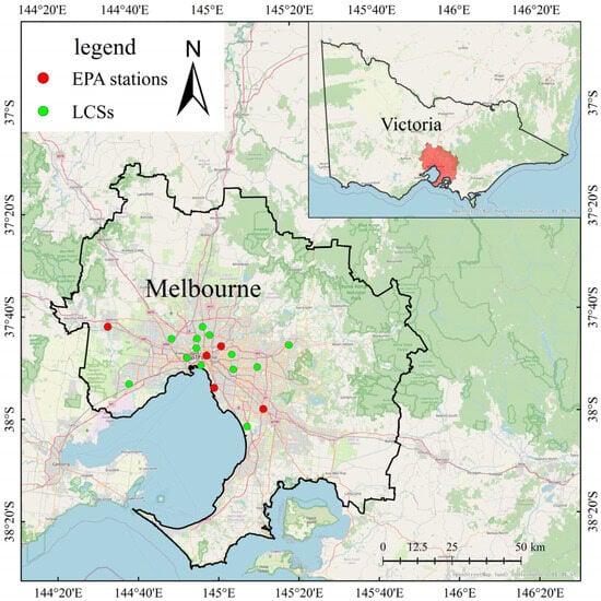
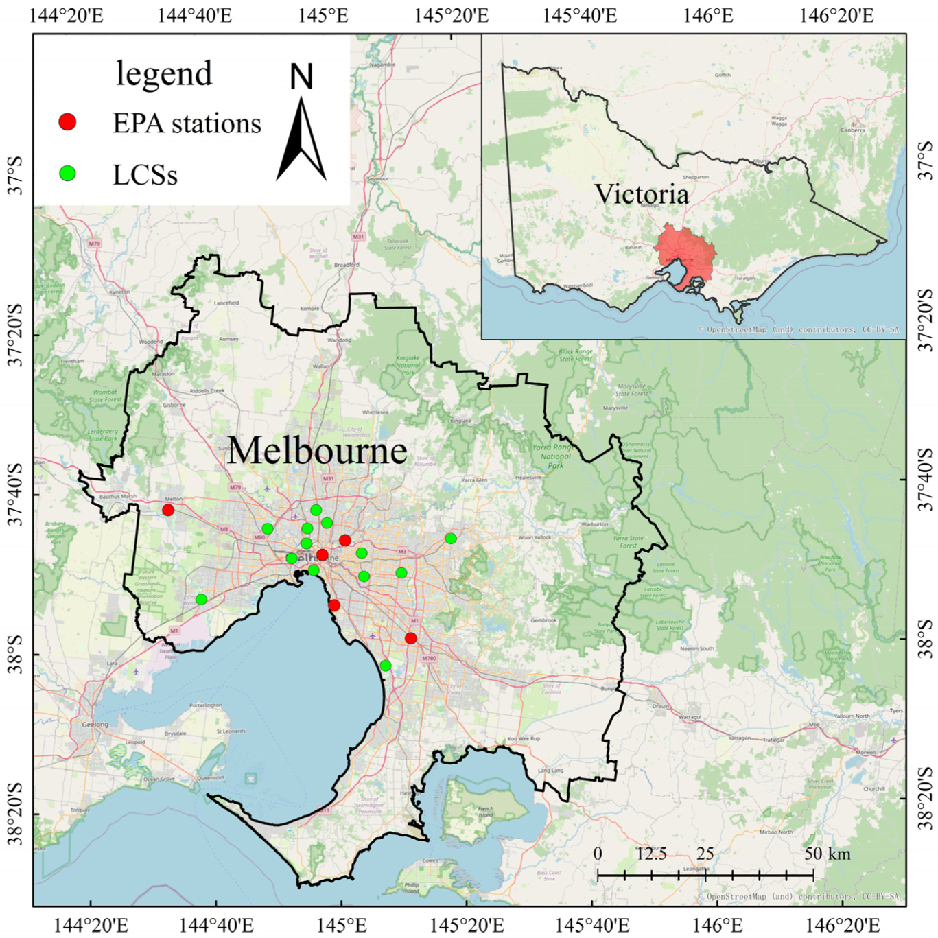
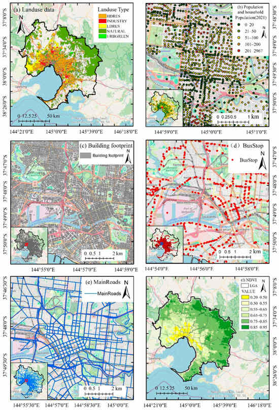
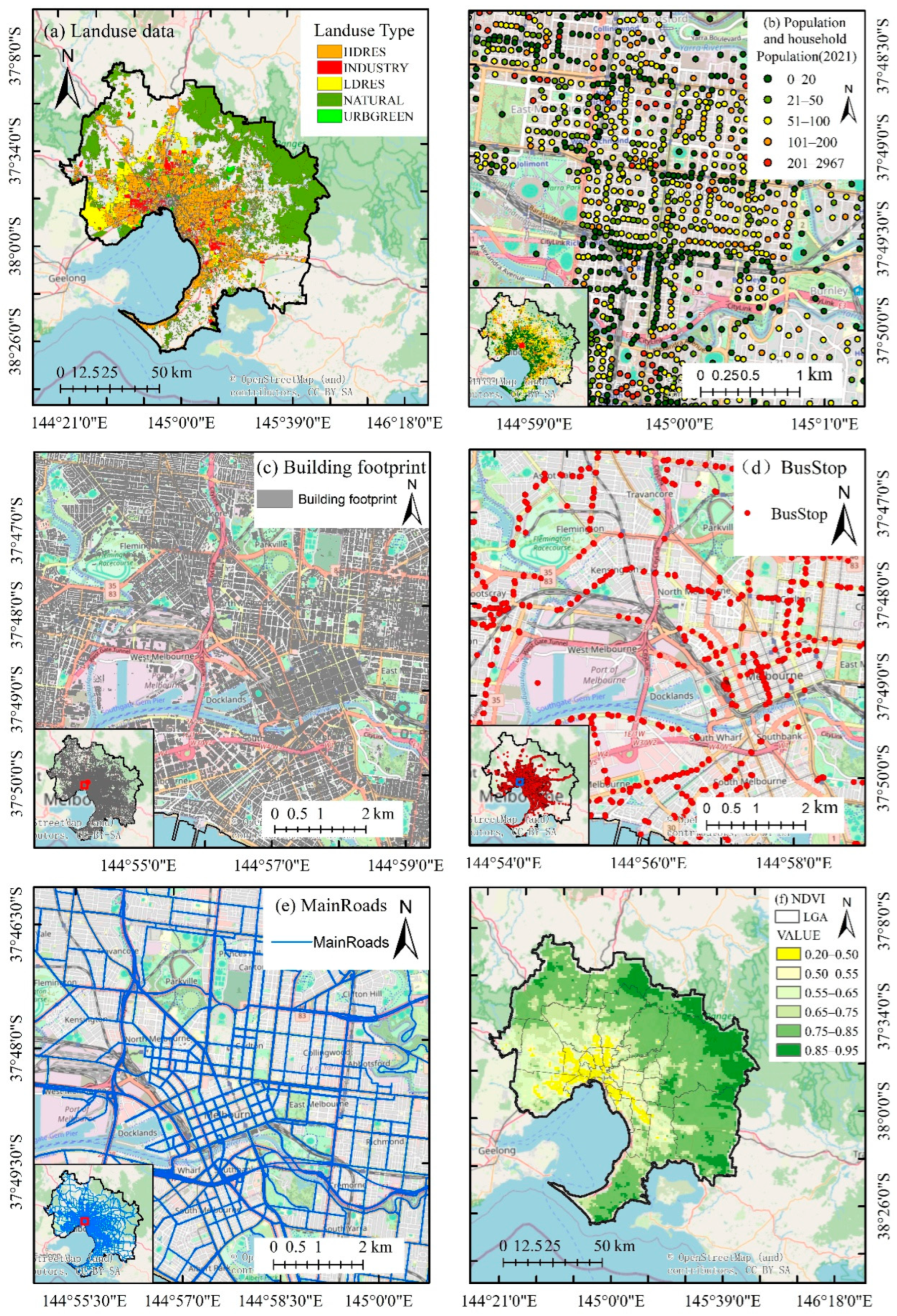
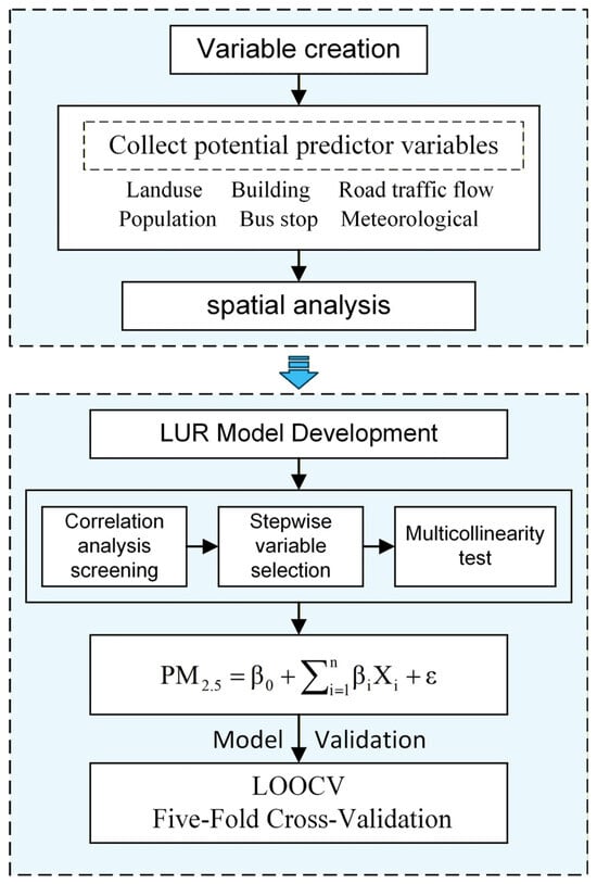
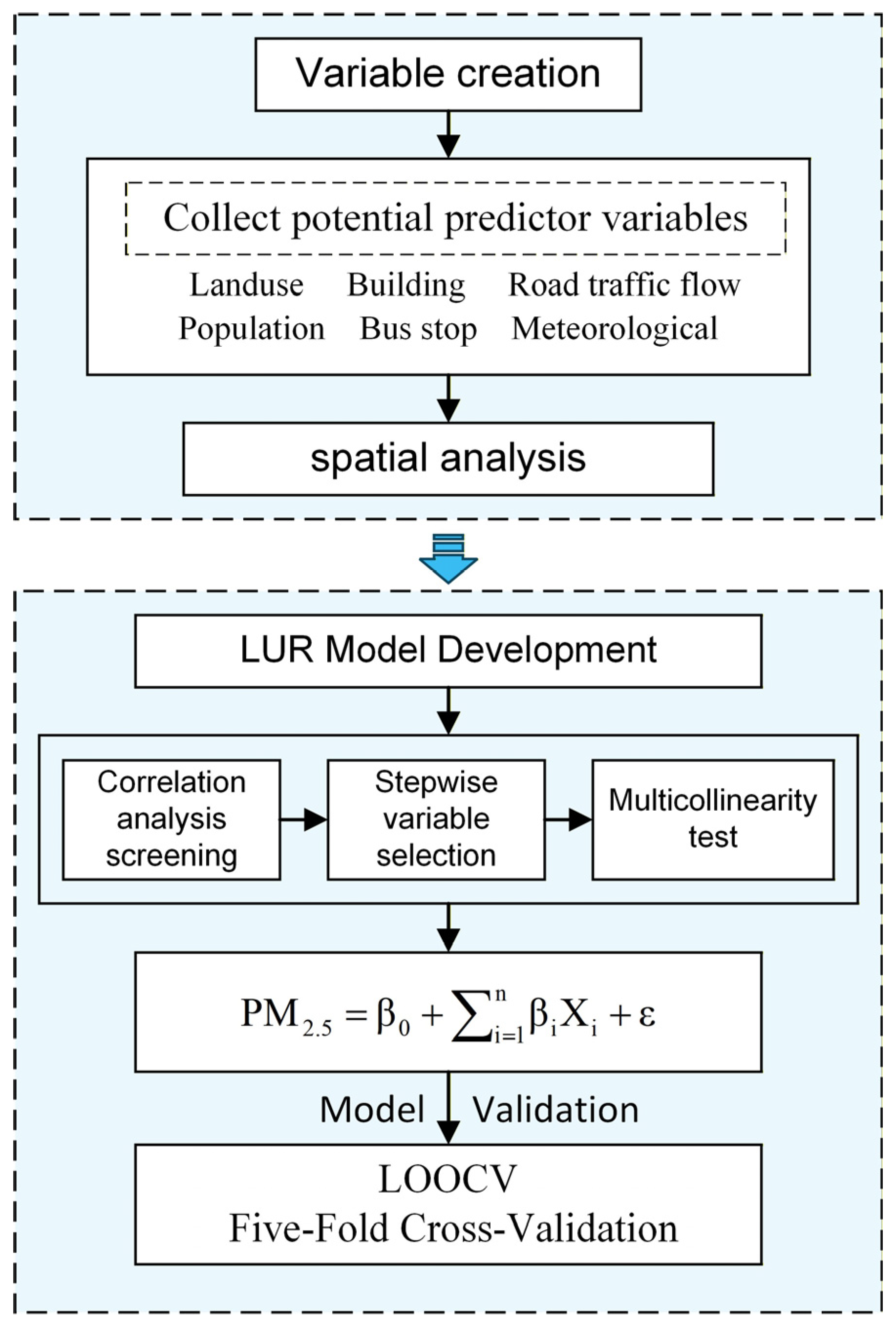
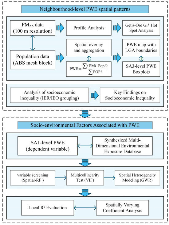
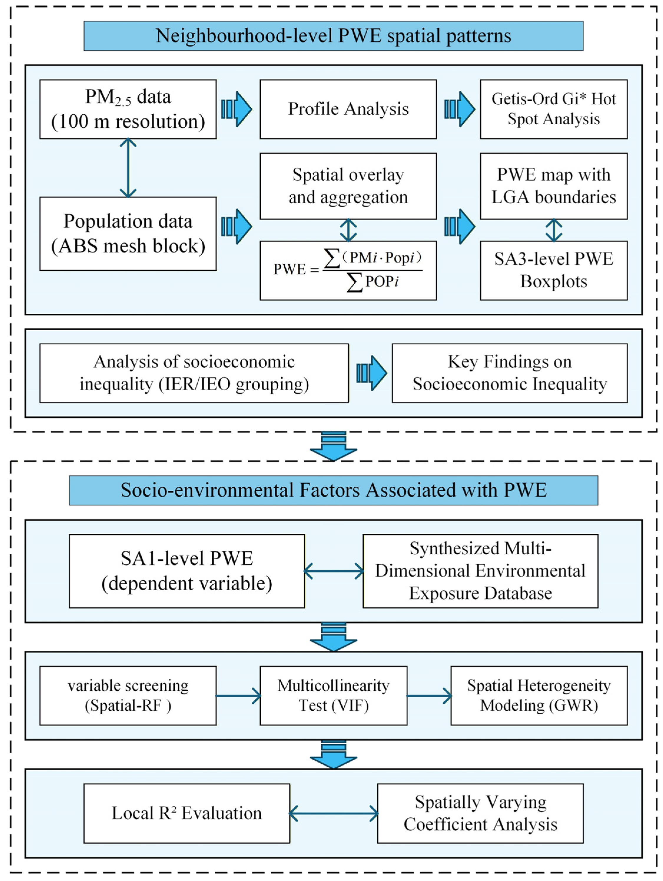
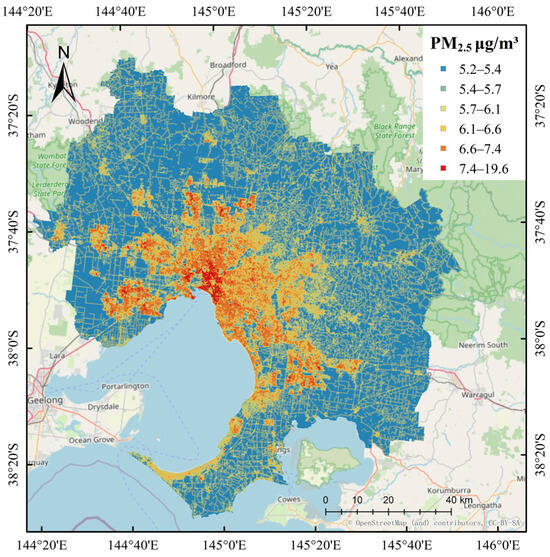
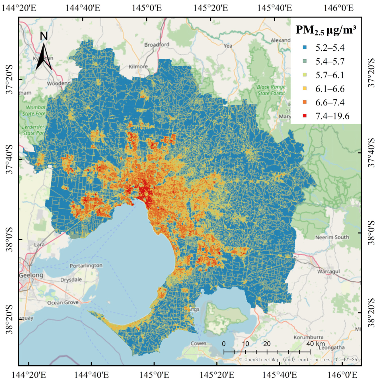
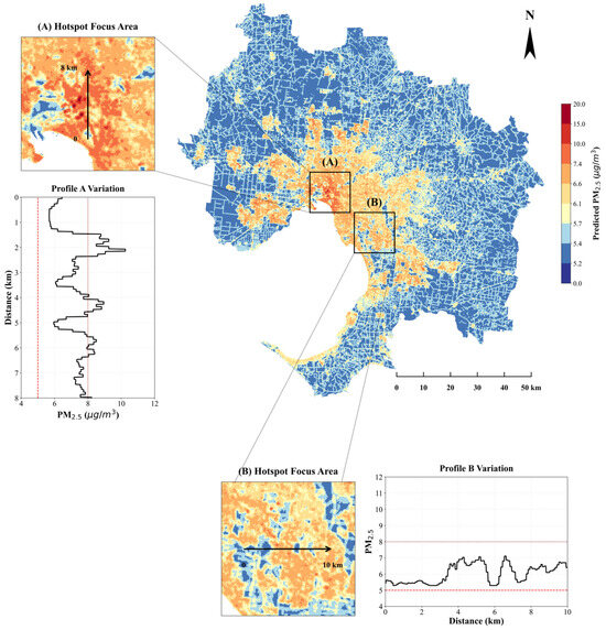
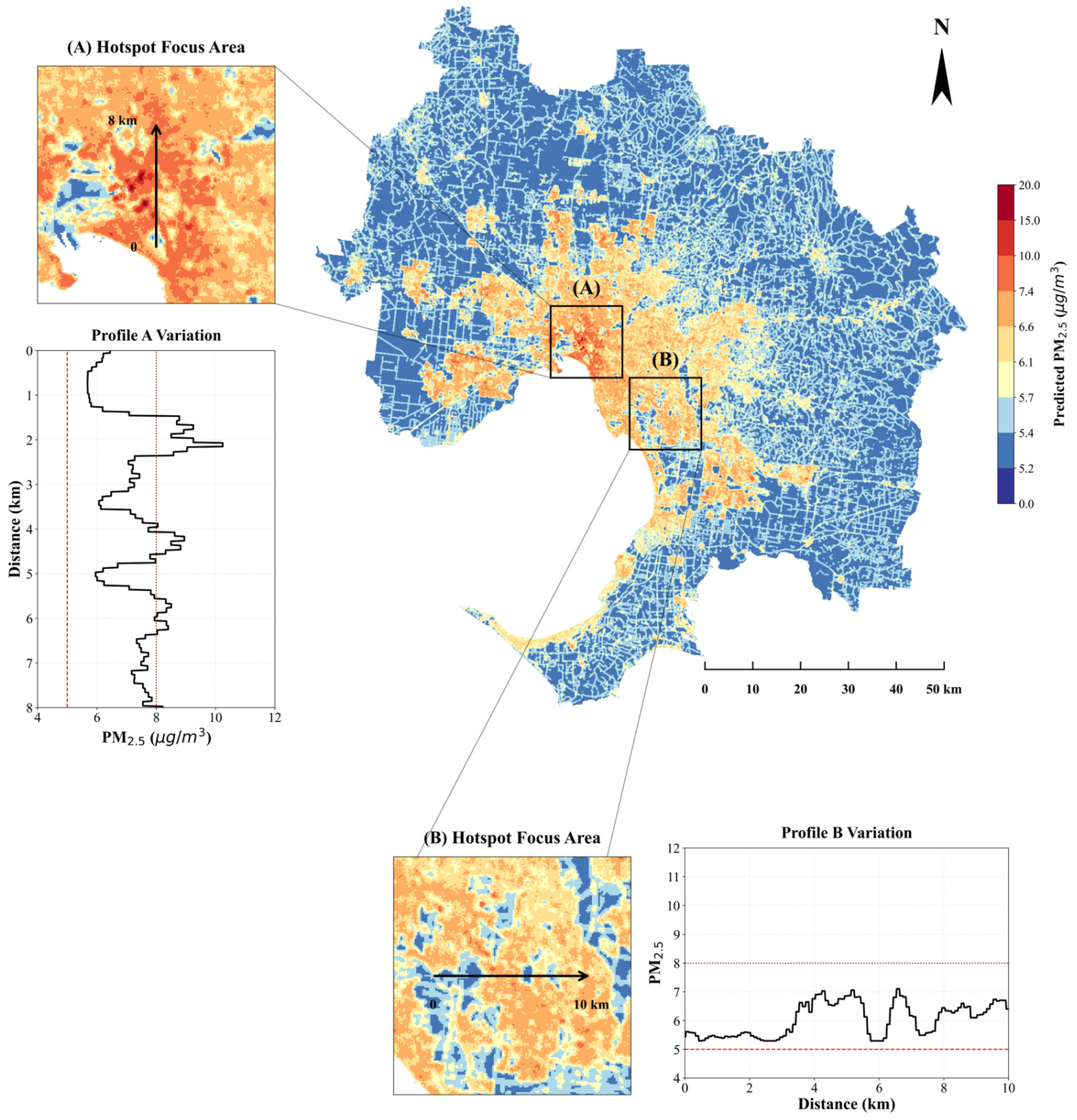
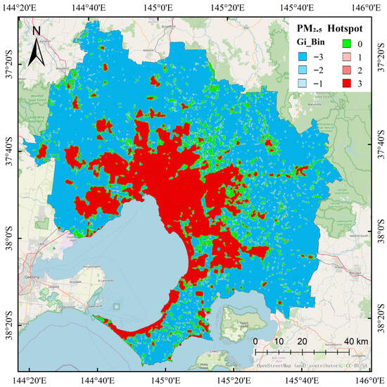
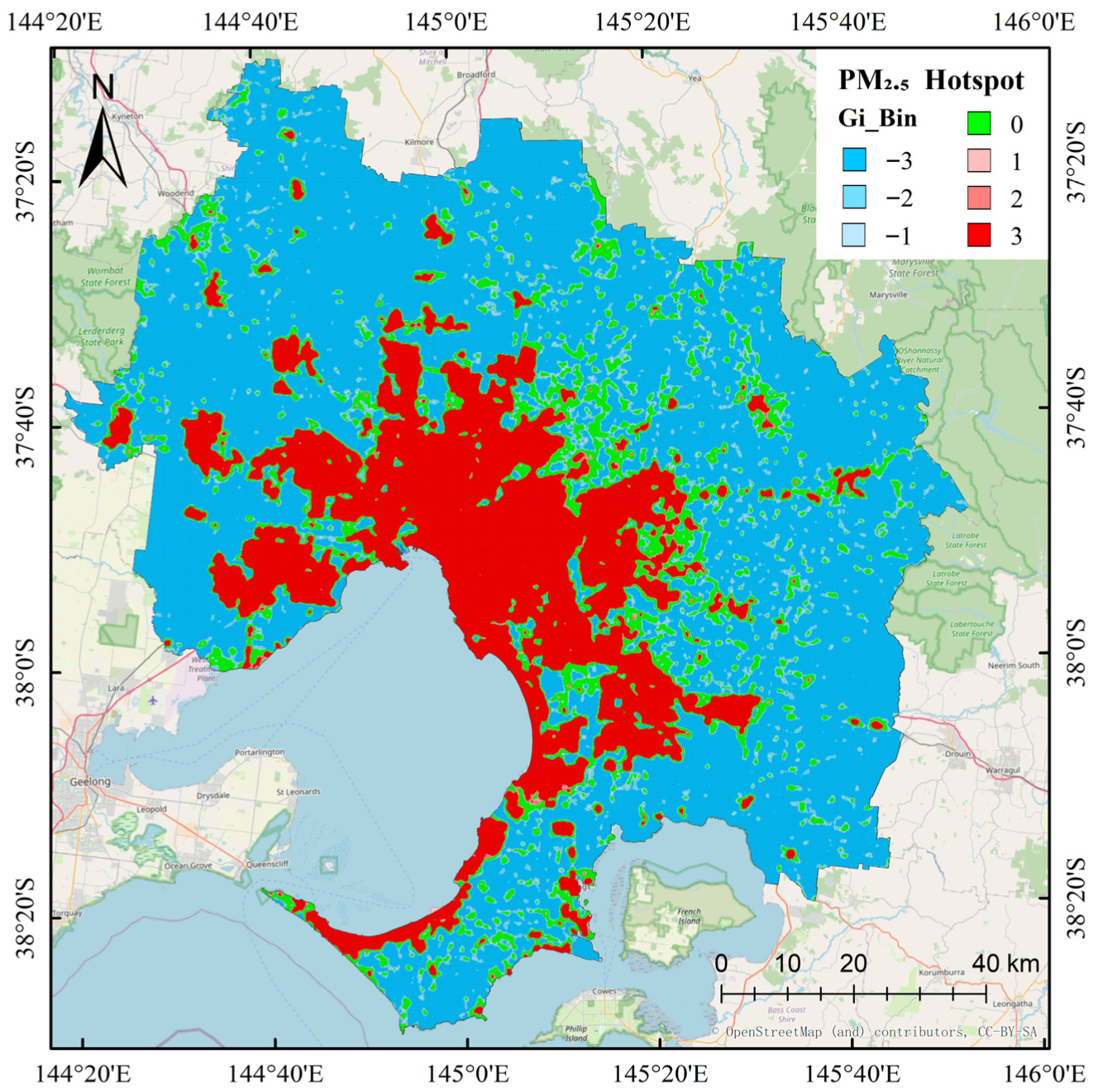
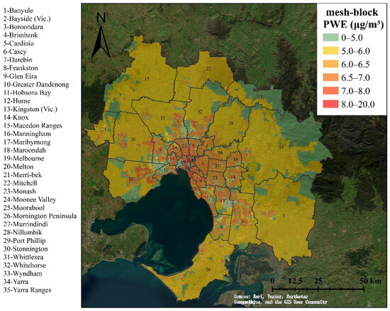
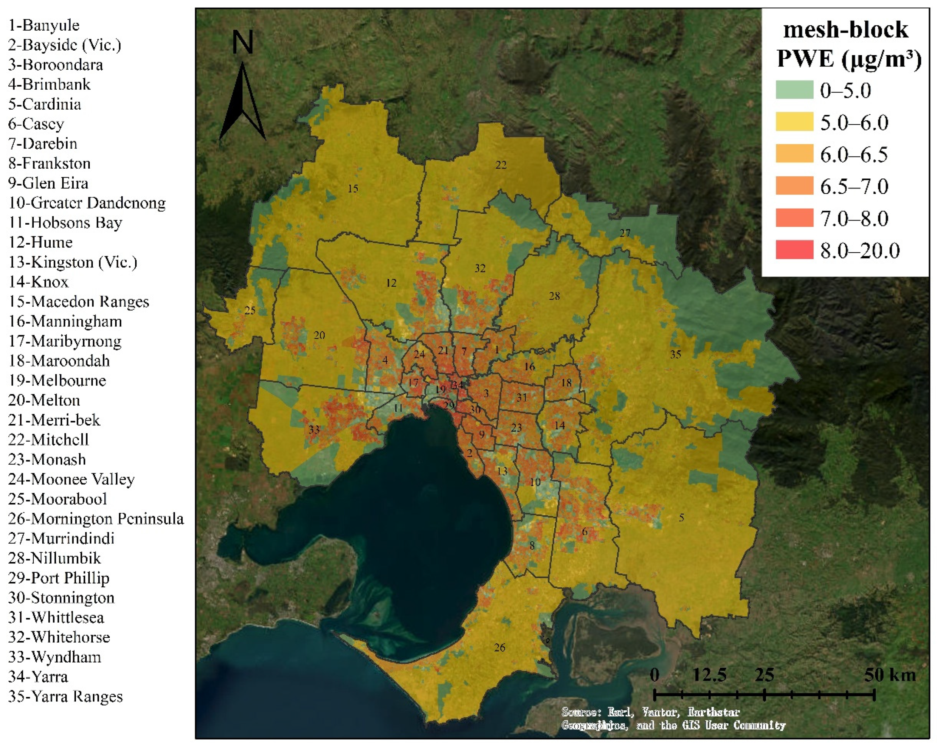
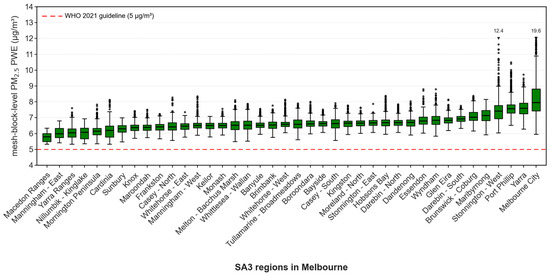
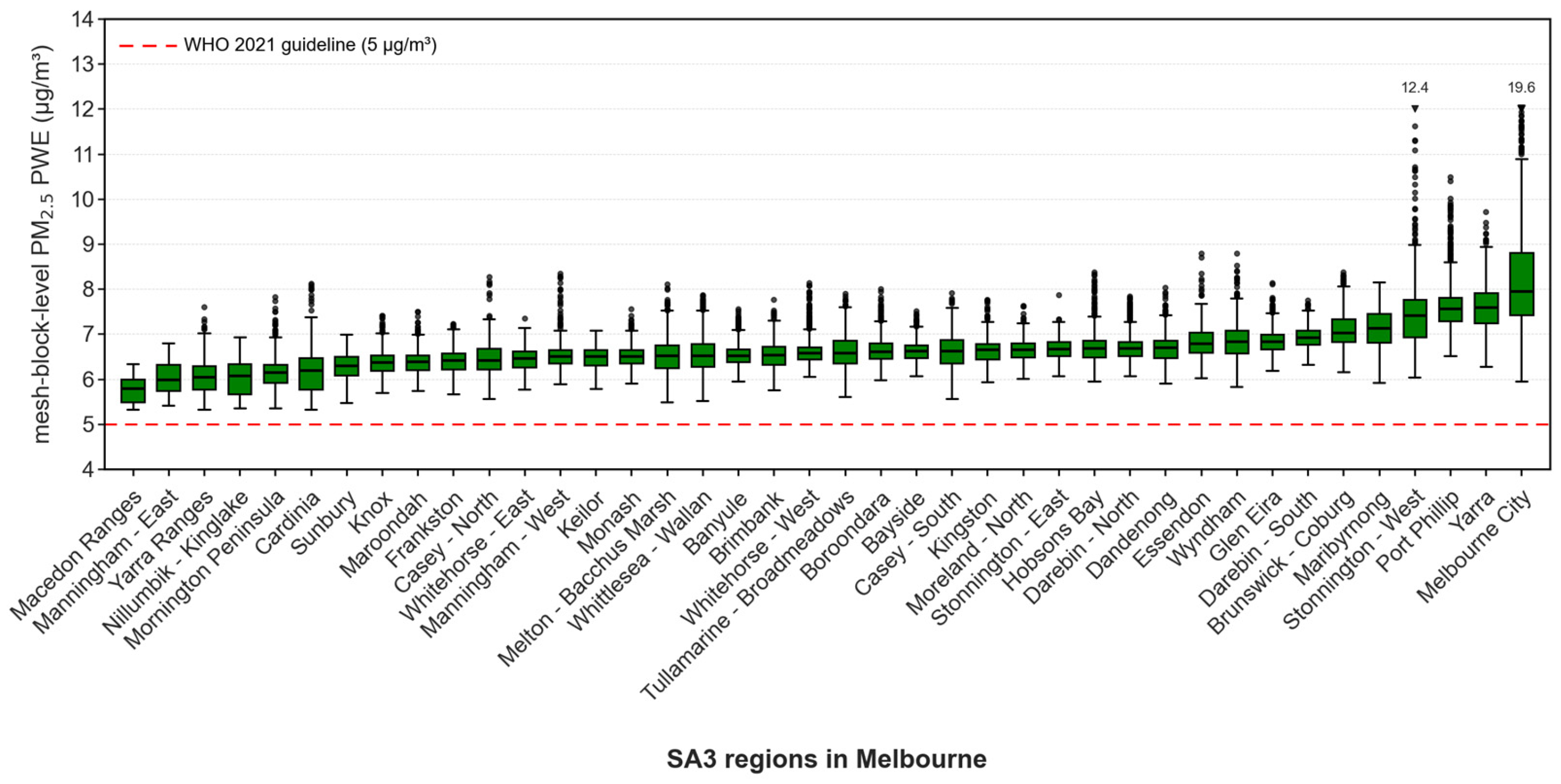
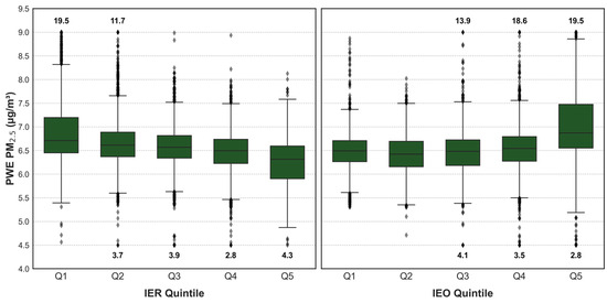
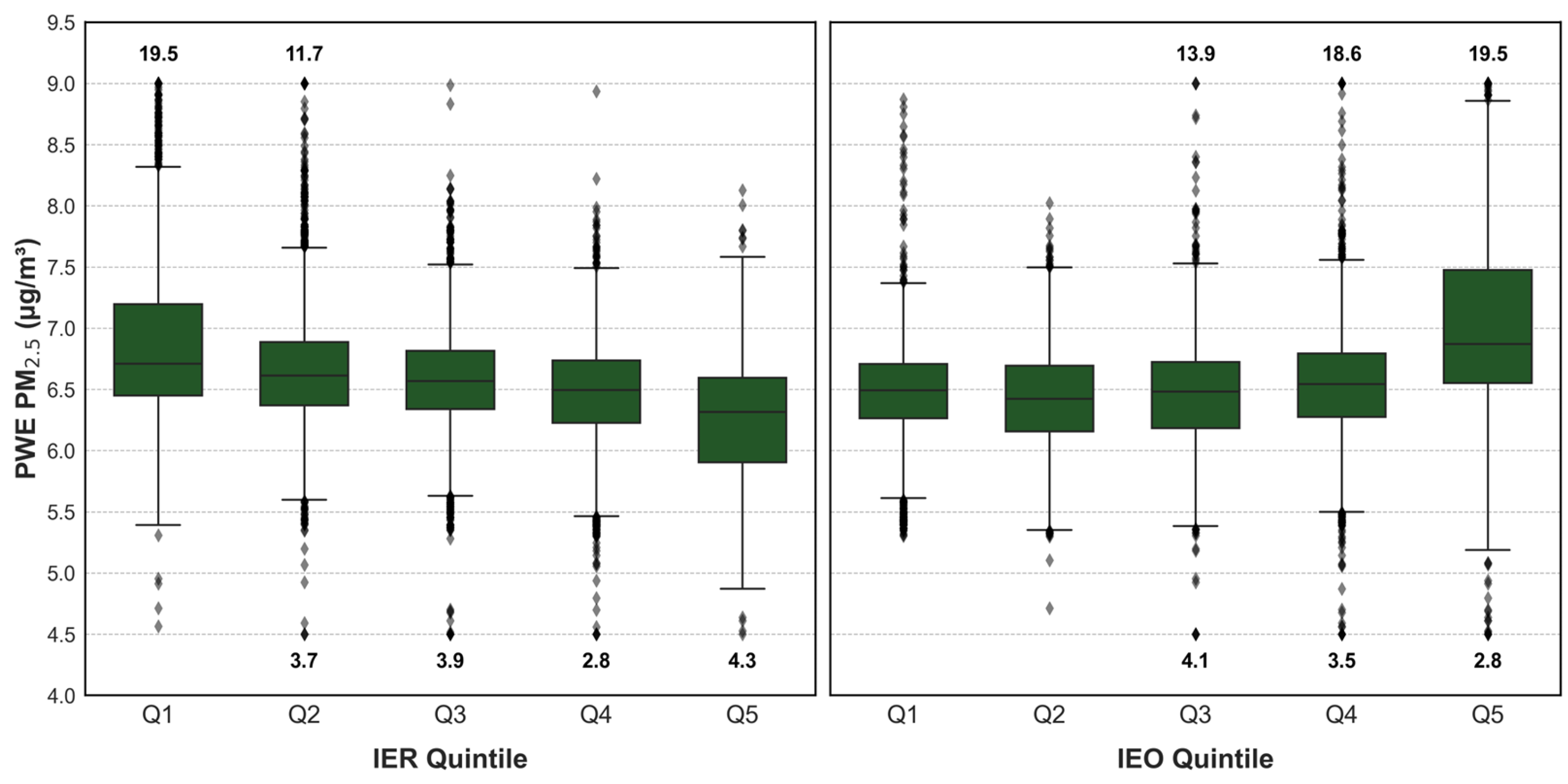
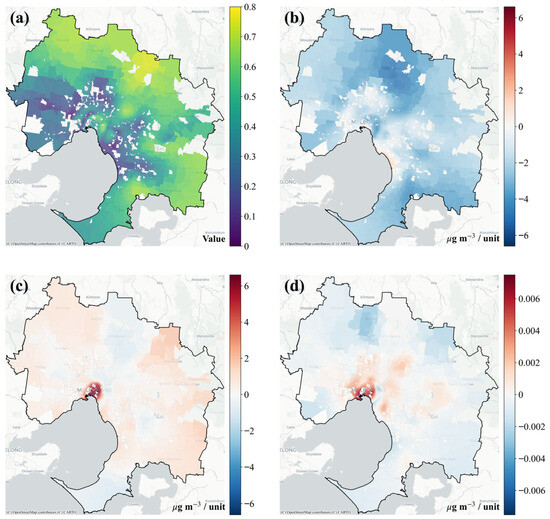
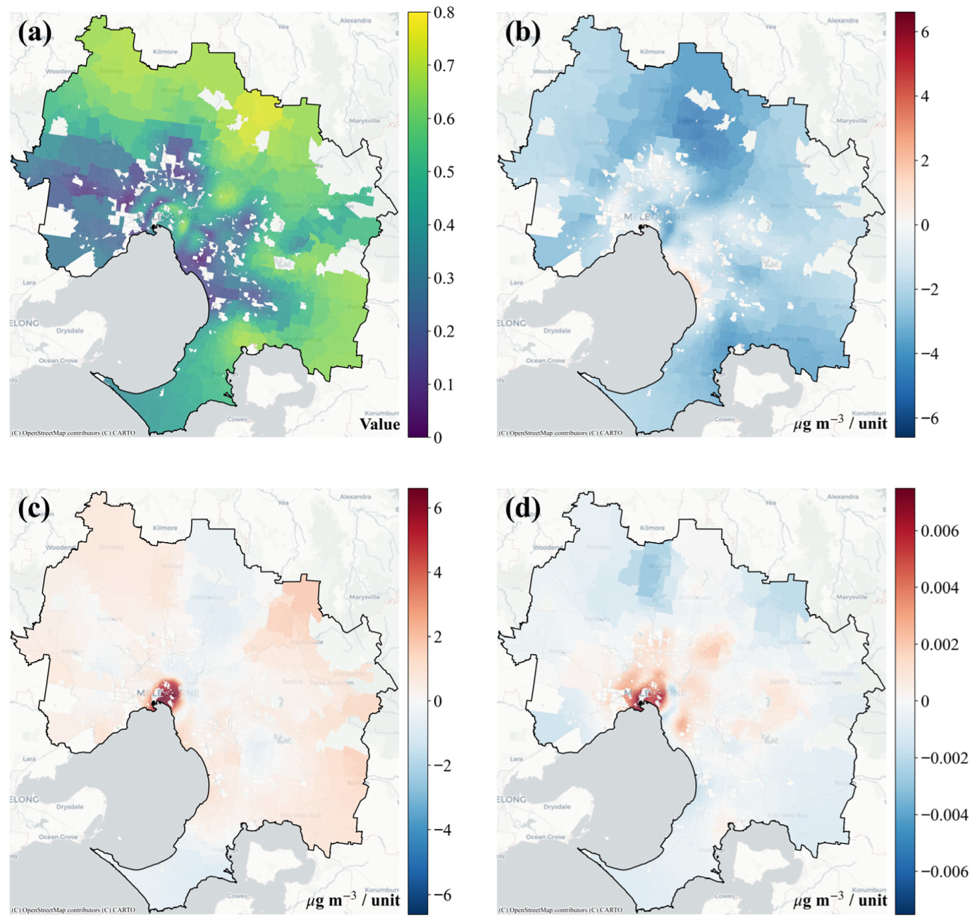

Disclaimer/Publisher’s Note: The statements, opinions and data contained in all publications are solely those of the individual author(s) and contributor(s) and not of MDPI and/or the editor(s). MDPI and/or the editor(s) disclaim responsibility for any injury to people or property resulting from any ideas, methods, instructions or products referred to in the content. |
© 2026 by the authors. Published by MDPI on behalf of the International Society for Photogrammetry and Remote Sensing. Licensee MDPI, Basel, Switzerland. This article is an open access article distributed under the terms and conditions of the Creative Commons Attribution (CC BY) license.