


Abstract
In this article, we introduce analogues of classic Euclidean bounds, including spherical caps, geodesic axis-aligned bounding boxes (AABBs), geodesic oriented bounding boxes (OBBs), and geodesic k-discrete oriented polytopes (k-DOPs). We also formulate k-circle coverage, a union of variable-radius caps solved by a binary integer program over candidates generated from Discrete Global Grid System (DGGS)-based rasterization. As all constructions run directly on the spherical surface, , they preserve geodesic distances and avoid projection distortion. We benchmark these methods on seven country boundary polygons consisting of thousands of points, and report construction time, memory, tightness, and query throughput. Results show our analytic geodesic bounds deliver orders of magnitude improvements over exact tests, with trade-offs in tightness: spherical caps are fastest but loosest; geodesic OBBs are a strong balance; geodesic k-DOPs consistently have the tightest bounds. k-circle coverage has spherical cap query speed while also having locally adaptive fits; construction time increases with DGGS resolution. Altogether, these bounds specific to the sphere provide practical, conservative filters for globe-scale Digital Earth queries.
1. Introduction
In geometric processing, geospatial queries, and rendering, bounding shapes are used as simplified proxies to encapsulate complex objects. By filtering out intricate geometric operations during collision detection or spatial indexing, these proxies significantly reduce computational overhead [1]. Bounding shapes have been studied extensively in both 2D and 3D Euclidean spaces [1,2,3]. For example, a typical collision-detection pipeline first checks whether the objects’ bounding shapes intersect. If the bounding shapes do not intersect, the more precise collision tests can be skipped, significantly improving the efficiency of the collision detection process [1]. In Geographical Information Systems (GIS), bounding shapes form the foundation of spatial indexing and broad-phase filtering, rapidly rejecting non-overlapping features before costly geodesic predicates are evaluated. This approach enables efficient handling of common geospatial tasks without excessive computational overhead.
The ideal bounding shape must balance tightness (conforming closely to the geometry) and simplicity (minimizing memory and computational cost) [1]. In 2D, classic bounding shapes include circles, axis-aligned bounding boxes (AABBs), oriented bounding boxes (OBBs), and k-discrete oriented polytopes (k-DOPs) [1,2], each offering trade-offs in computational cost, memory usage, and tightness of fit.
In spite of the abundant literature on the construction of bounding shapes in 2D and 3D Euclidean spaces [1,3,4,5,6], a considerable gap remains in developing bounding shapes defined directly on the globe as a spherical surface. Many GIS and graphics pipelines perform broad-phase indexing and culling in a planar space (e.g., storing geometries in projected coordinates) because these structures are fast and widely supported. However, any planar projection introduces systematic distortions in distance and area [7,8,9], since mappings from the sphere to the plane are not isometric (they do not map distances and angles exactly). These distortions bias intersection tests unless computationally expensive corrections are applied. Moreover, such methods can be computationally slower depending on the type of projection applied, such as area-preserving projections [7,10]. Our work addresses this by developing bounding shapes within the spherical domain, specifically for large-scale vector data in Digital Earth frameworks [11].
Geospatial vector data often contain thousands or even millions of spatial features, making fast and efficient query handling essential for scalable analysis. For example, when managing the geographic boundaries of large regions, such as countries or provinces, bounding shapes enable rapid retrieval of all relevant spatial features within these areas. Our goal is to provide rapid spatial query evaluations, significantly improving performance in large-scale geospatial datasets.
In this paper, we introduce novel geodesic analogues of the basic Euclidean bounding shapes. We evaluate complex geospatial polygons under a variety of metrics, including construction time, memory usage, tightness, point-in-polygon test, and polygon–polygon intersection time. Our experiments show that the circle, represented as a spherical cap in spherical geometry, produces the fastest intersection test and the least memory usage of the bounding shapes constructed. Geodesic k-DOPs consistently achieve the tightest bounds. While geodesic OBBs offer a decent trade-off between performance and tightness, geodesic AABBs consistently underperform due to their inflexible alignment with defined coordinate axes. The consequence is severe distortion, making geodesic AABBs an unsuitable choice for bounding shapes on the sphere. Unfortunately, all these polytope-like bounds generally remain too slow at test time for the point-in-polygon and polygon–polygon intersection tests. On the sphere, a cap is defined by a centre and angular radius, so intersection reduces to a single dot-product threshold, whereas axis-aligned or other polygons require multiple great-circle half-space tests with extra normalization, which are inherently more complex than on the plane.
To overcome these limitations, we propose k-circle coverage.
In this work, we reformulate the original variable-radius covering problem (which exhibits combinatorial explosion as the number of subsets grows [12]) into a binary integer linear program (BILP). Complex polygons are approximated using a set of multiple optimally located variable-radius spherical caps in order to attain significantly more accurate coverage. The main challenge is finding the best number, location, and size of circles to tightly fit complex shapes. We employ the Discrete Global Grid System (DGGS) for discretization, turning the continuous problem into a discrete one. Our approach draws inspiration from the classic set-cover problems and recent developments in multi-circle coverings on the plane [12,13,14], but we adapt them to geodesic domains.
We found that k-circle coverage outperforms traditional geodesic bounding shapes and offers tighter bounds for complex geospatial objects. It is also compatible with rejection-based filtering in our tests. From a computational perspective, point-in-polygon and polygon–polygon intersection calculations were significantly faster than the preliminary DGGS-based pre-processing phase. Nonetheless, our method remains compatible with DGGS for hierarchical indexing or cascaded filtering when required.
In summary, this paper offers:
- Geodesic bounding shapes on spherical surfaces (): Formal definitions, analysis, and linear-time constructions for spherical caps, geodesic AABB/OBB, and geodesic k-DOPs.
- k-circle coverage: Introduction of k-circle coverage on the sphere and a novel DGGS-discretized, BILP-solved union-of-caps with conservative coverage guarantees on sampled vertices.
- Efficient predicates: Constant- or near-constant-time point-in-polygon and polygon–polygon intersection tests tailored to , suitable for broad-phase culling.
- Comprehensive evaluation: Empirical analysis of time, memory, tightness, and throughput on six real polygons (3k–12k vertices) with a reproducible setup.
2. Background and Prior Work
This section contextualizes the theoretical and methodological foundations of this study. We review bounding shapes implementations in classic Euclidean forms to neural bounding implementations that leverage learning-based models, and examine how bounding shapes have been integrated into spatial indexing schemes such as R-trees, S2, and H3. We also describe the shortcomings of projection-based methods that approximate spherical data using planar methods and describe the Digital Earth paradigm of DGGS and summarize its approach to discretization, indexing, and query primitives that we later use as a benchmark model of our comparisons. Finally, we summarize the mathematical concepts in spherical geometry that underlie our geodesic constructions.
2.1. Approaches to Bounding Shapes
In local-scale GIS contexts, planar bounding boxes typically suffice because projection-induced distortions are minimal. At global scales, however, these distortions become non-negligible, making it necessary to use geodesic lines on the Earth’s curvature. While many projections can still yield topologically valid bounds away from singularities (locations where the map projection is undefined, e.g., the poles in many projections), they can degrade tightness and increase computational cost. These global use cases motivate the construction of spherical bounding shapes.
One simple approach to define spatial computations on a spherical surface is to project the spherical dataset into the Euclidean domain through map projections [15]. Here, we compute bounding shapes in flat space with conventional methods before inverse-projecting back to the sphere. Possible projections in Digital Earth paradigms include gnomonic or Snyder projections [7], or the exponential map [16,17]. However, such projections inevitably introduce distortions in the final bounding shapes, especially near the poles or along coordinate axes. Illustrations of these distortions are shown in Figure 1, applied to a dataset that represents the boundary of Australia.
Figure 1.
Projection-induced distortion for Australia. Planar mappings from to are non-isometric and do not preserve geodesic distances or angles. Although planar bounds may look tight in projection, they distort the true spherical shape and can fail to fully cover the region. This can introduce false negatives in broad-phase spatial queries.
Another approach is to use 3D bounding boxes in their original Euclidean domain for spherical datasets [1]. Although simple to construct, these volumes often include large regions of empty space when the data is restricted to the surface of the sphere. Latitude–longitude boxes [18] are also commonly used, but their edges consist of small-circle arcs (parallels) and great-circle arcs (meridians). A nontrivial challenge arises when extending latitude–longitude boxes into OBB or k-DOP counterparts, as the edge directions are no longer constrained to constant latitude or longitude. In practice, this often introduces complex rhumb (loxodromic) lines, which are not geodesics except along the equator and meridians, and complicate both the representation and the algorithms that operate on the shape.
2.2. Analytic Bounding Shapes
Classic Euclidean bounding shapes such as minimum bounding circles [6,19], axis-aligned bounding boxes (AABBs) [1,20], oriented bounding boxes (OBBs) [1,2,5], and k-discrete oriented polytopes (k-DOPs) [1,4,5] offer well-established trade-offs between computational efficiency and geometric tightness. While bounding circles and AABBs are inexpensive to construct and query, they often suffer from excessive empty space and orientation bias, leading to high false-positive rates. OBBs and k-DOPs mitigate this by aligning with the dataset’s variance or utilizing multiple orientations, yielding tighter bounds at the cost of increased construction complexity and storage. Furthermore, rigid Euclidean constructs like AABBs rely on uniform metrics that do not naturally translate to spherical space.
To overcome the limitations of forcing a complex object into a single, global primitive, our k-circle coverage models a polygon as a union of localized spherical caps. Motivated by classical variable-radius covering problems in planar geometry [12], this flexible, feature-adaptive approach has not been previously extended to the sphere.
2.3. Learning-Based Bounding Shapes
Recent neural approaches have proposed learning bounding shapes directly, replacing analytic primitives with classifiers or implicit fields that label points in (or on ) as inside or outside [21,22,23,24,25,26]. These methods can lower false positives in specific benchmarks by tailoring decision limits to a given object and query distribution. However, for our geospatial setting, this strategy is disproportionate to the problem. First, learned bounds are typically specialized: each object class, query type (ray–shape intersection vs. point containment), and domain (planar vs. spherical) tends to require a distinct network, each with non-trivial training time, tuning, and dataset construction.
More critically, most current learning-based bounds lack formal guarantees of conservativeness (i.e., containing all the points). Zero false-negative behaviour is typically supported empirically (e.g., through Monte Carlo sampling) rather than by proofs of coverage [21]. This limitation is particularly problematic for GIS frameworks that depend on strict correctness, as even a single missed point (i.e., a false negative) violates the core purpose of a bounding shape as a rejection test.
These trade-offs motivate our use of analytic, geodesic bounding shapes with demonstrable containment on . Our implementations rely on closed-form algorithms, are easily reproducible, and offer strict no-false-negative guarantees by construction. We find in practice that they offer sufficient pruning efficiency without the expensive training, ambiguity, and validation problems in these learning-based approaches.
2.4. Bounding Shapes in Other Spatial Frameworks
Most spatial frameworks employ a filter-and-refine strategy: inexpensive bounding shapes accelerate queries by discarding non-overlapping candidates before expensive exact geometry tests are performed.
The R-tree family [27] packs spatial objects in a height-balanced tree whose nodes hold minimum bounding rectangles (MBRs). Query performance heavily depends on the quality of these bounds. Variants such as the R*-tree [28], Hilbert R-tree [29], and SR-tree [30] improve clustering, reduce overlap, or combine multiple bounding shapes (e.g., rectangles and spheres). Collectively, these trees demonstrate that bounding shape quality—tightness, orientation, adaptability to variation in the data—is a significant factor in index efficiency.
For global-scale applications, planar projections introduce severe distortion. Systems such as Google’s S2 Geometry Library [31] and Uber’s H3 system [32] instead use hierarchical spherical grids. S2 subdivides a cube projected onto the sphere into spherical quadrilaterals, while H3 uses a hexagonal tesselation derived from a base icosahedron. In both cases, fixed-resolution cells act as coarse filters during query traversal.
Our approach diverges from these hierarchies by focusing on feature-adaptive bounds defined continuously on . This allows them to rotate and align specifically with the principal axes of the input geometry, offering arbitrary precision independent of a grid resolution. Furthermore, our k-circle coverage formulation introduces a hybrid novelty: it leverages the discrete nature of DGGS for tractable candidate generation (solving the coverage location problem) but outputs a continuous union-of-caps representation. This decouples the runtime query phase from the grid hierarchy, enabling constant-time intersection tests that do not require traversing a cell tree or managing discrete cell collections.
2.5. Spherical Geometry
This section establishes the notation and core concepts of spherical geometry, which we use through Section 3 and Section 4, and the analyses that follow.
Points on the unit sphere are represented as unit vectors in three-dimensional Euclidean space :
A great circle is the intersection of the unit sphere with any plane that passes through the origin. On the sphere, geodesics are exactly great circles—the shortest path between any two of its points lies entirely on the circle itself. Consequently, all geodesics on are great circles. The geodesic distance between two points and on the sphere is defined as the central angle between them:
This metric accounts for the curvature of the sphere and is essential for accurate geodesic bounding shape computations [33].
Finding a point set’s angular extents along prescribed orientations is a fundamental step in the construction of geodesic bounding shapes in Section 3. Choose an orthonormal pair that spans the target great-circle plane, whose normal is . Project each point onto this plane and measure its oriented central angle
Each value is the signed arc-length (in radians) from the reference axis to the projection of p onto the great-circle plane, measured counter-clockwise about the normal .
A spherical lune is the intersection of two hemispheres whose boundary arcs meet along a pair of antipodal points. Fix two distinct great-circle planes through the origin with unit normals . Each plane subdivides the sphere into hemispheres with outward normals and . A spherical lune is formed by intersecting one hemisphere from each plane; its pole directions are
Informally, it is the football-shaped patch “wedged” between two great-circle half-arcs that share common endpoints. An example is illustrated in Figure 2, where the shaded blue region denotes the smaller lune bounded by the red and blue great circles. Spherical lunes will reappear throughout the paper, as many of these bounding shapes on can be expressed succinctly as intersections of spherical lunes.
Figure 2.
Illustration of a spherical lune—the shaded blue region shows the smaller intersection between two hemispheres whose bounding great circles (blue and red) meet along antipodal points on the sphere. The normals and define the planes of these great circles, and their cross product gives the pole direction .
2.6. Multi-Disk Covering in the Plane
Early planar coverage models, such as the Location Set Covering Problem and the Maximal Covering Location Problem [34,35,36,37], assumed fixed-radius disks to cover points of interest. Subsequent generalizations explored variable radii, initially optimizing a single global radius parameter [38,39], and later allowing independent radius selection for each disk to better adapt to spatial demand [40,41,42,43].
The most direct precursor to our approach is the Variable Radius Covering Problem introduced by Berman et al. [12]. In its discrete form, the decision-maker selects both the number of disks and their variable radii to completely cover all points of interest at a minimal total cost. By restricting candidate locations to precise sites, Berman et al. framed this flexibility as a mixed-integer programming problem, balancing smaller, cheaper disks against fewer, larger ones.
Crucially, all of these classical models operate strictly within Euclidean geometry. We adapt this discrete variable-radius template to formulate our novel k-circle coverage on the unit sphere. In our approach, candidate disk centres are restricted to DGGS refinement vertices, ensuring the resulting spherical caps align with and collectively cover the polygon’s DGGS rasterization. We retain the binary-integer framework to enforce a maximum budget of k caps, but rather than assigning an explicit cost to radius size, we fix each chosen radius to the minimum value required for local containment and strictly penalize the enclosure of non-polygon cells. All distance and coverage predicates are evaluated directly on .
2.7. Discrete Global Grid System (DGGS)
Discrete Global Grid Systems (DGGSs) partition the Earth’s surface into hierarchical, multi-resolution cells through the recursive refinement of a base polyhedron [9,11,44,45,46]. By utilizing geodesic great-circle arcs, these grids provide topologically consistent, uniform coverage that conforms directly to the sphere, avoiding the severe planar projection distortions that occur at global scales. A visualization of the refinement process of an icosahedral geodesic DGGS from resolution 0 to 5 is shown in Figure 3. In this paper, we leverage a geodesic DGGS to discretize the continuous k-circle coverage problem into a tractable grid-based formulation.
Figure 3.
The refinement of the geodesic DGGS grid from resolutions 0 to 5. The highlighted triangle is a base cell of the DGGS [44].
To generate candidate bounding caps, spherical polygons are first rasterized into DGGS cells. Each polygon vertex is identified within a specific triangular base-cell of the high-resolution polyhedral proxy. The geometry is then mapped onto the planar face using a piecewise gnomonic projection, which preserves geodesic edges as straight lines to allow for efficient planar computation. As each polygon edge is processed, the polygon is rasterized by encoding all DGGS cells that either contain its vertices or intersect its edges. This approach respects spherical geometry, minimizes distortion, and allows for the constant-time encoding required to build the discrete candidate set for our high-resolution Digital Earth platforms [45].
3. Constructing Geodesic Bounding Shapes
Throughout this section, we assume the input to each bounding shape construction is a finite set of points
represented as unit vectors in . Each denotes either a vertex of a spherical polygon or an element of a point cloud sampled on the unit sphere. The memory structure of all bounding shape classes follows the data representations recommended in [1]. Memory use remains low across all bounds, with spherical caps smallest, AABBs and OBBs slightly larger, and k–DOPs scaling linearly with k yet staying lightweight when directions are shared. For a visual comparison of all bounding shapes on the same dataset (Mainland Australia), see Figure 4; we will refer to it throughout this section.
Figure 4.
Bounding shapes for mainland Australia (relative area in parentheses).
3.1. Minimum Spherical Cap
A spherical cap is the region of the unit sphere defined by a centre and a dot-product threshold , namely
which corresponds to all points lying within a central angle of the apex direction u. The goal of this construction is to compute the smallest such cap that encloses a given point set . Figure 5 illustrates this geometric definition, showing how the angle and threshold t determine the boundary of the cap.
Figure 5.
Illustration of the spherical cap : the black circle represents the sphere’s silhouette, the blue arc indicates the visible rim and central angle , the red rays extend to boundary points p and , and the threshold t is marked along the u-axis where .
Our algorithm leverages a well-established Euclidean strategy—computing the minimum enclosing ball in —as a proxy for spherical cap construction. We interpret the unit vectors as points in and apply Welzl’s algorithm for the smallest enclosing ball [19]. As part of the process to ensure expected linear time, the point set is shuffled once using a fixed pseudorandom generator. Welzl’s algorithm then returns a unique minimal Euclidean sphere centred at with radius that contains all points of P.
To convert this Euclidean ball to a spherical cap, we first compute the norm . If this norm is negligibly small, the centre is effectively the origin of the unit sphere, meaning the input points are widely distributed and all directions are acceptable. The cap in this case shrinks to the whole sphere. Otherwise, we normalize the centre to obtain the cap axis . Solving for on the boundary yields:
which ensures that for all , and is tight for any support points that lie exactly on the boundary of the Euclidean ball. This yields the spherical cap that minimally encloses the input points, as illustrated in Figure 6.
Figure 6.
Intersection of spheres for cap threshold. The black circle outlines the unit sphere, the blue circle marks the minimum enclosing sphere. The red segment marks the offset from the origin to the cap plane; dashed lines show the two radii.
The cap is stored compactly as the pair , taking only 32 bytes in double-precision floating point—a scalar for each of the three values in the unit vector u and a scalar threshold quantity t. The complexity is overall with auxiliary memory. This conversion is numerically stable provided the inputs are in double precision. Degenerate configurations (e.g., nearly hemispherical or antipodal inputs) are handled by treating small as the full-sphere case.
A spherical cap is defined by one dot-product inequality and is thus the simplest bounding primitive in . This makes the structure particularly well-adapted to coarse filtering or to preliminary pruning phases. However, because the cap is radially symmetric, it may not capture elongated or skewed point distributions efficiently.
3.2. Geodesic AABB
The geodesic AABB construction begins by establishing a fixed orthonormal frame using two basis vectors:
and completes a right-handed frame with
All angular measurements are taken with respect to this frame; no run-time rotation of the coordinate system is required.
For each input vertex , we compute two signed angles with atan2:
Their extrema at these angles:
determine four great-circle half-spaces.
The two half-spaces form a longitude-style lune , while the two half-spaces form an independent latitude-style lune . Four lines are formed by intersecting the half-spaces, each of which can point in two opposite directions. For each boundary plane, we retain the orientation that encloses all input points.
Since the axes are fixed to the meridian planes, edges converge to skew ‘kite’ corners. The footprint grows especially for oblique or high-latitude shapes and into the antimeridian. By fixed orientation, we mean that the principal axes remain constant during computation. This constraint often leads to looser encodings compared to geodesic OBB or geodesic k-DOP counterparts which adapt their orientation for tighter fits.
The memory usage consists of storing only the minimum and maximum corner directions, each costing bytes. Construction requires a single pass over P, i.e., linear time, .
3.3. Geodesic OBB
The geodesic OBB generalizes the axis-aligned construction by rotating the frame to match the principal components of the input data.
We begin by computing the covariance matrix of the point set and extracting its eigenvectors. The two corresponding to the largest eigenvalues define the principal directions we need. Let and denote these dominant directions. Complete a right-handed triad with
For each vertex , we compute the two signed angles that define perpendicular lunes:
Their extrema determine two perpendicular spherical lunes, exactly as in the geodesic AABB case but now aligned with the principal component frame. The resulting bounding directions are returned and denoted as
Since principal component analysis aligns the box frame to the dataset’s principal directions, the angular half-extents around each axis are balanced. At the sphere, every corner is the point of intersection between some great-circle edge (rotated longitude constant) and some small-circle edge (rotated latitude constant); in terms of the half-extents as and , the dihedral angle between the supporting great-circle planes at the corner is
which approaches for balanced, large extents. Intersecting the half-spaces gives four lines, each of which can point in two opposite directions. We keep the orientation that still encloses the original geometry—specifically, the direction that points roughly the same way as the average of all edge normals—so we end up with the correct four lines and discard their antipodal counterparts.
The data structure stores the centre bytes, two principal components bytes, and two half extents bytes, occupying 88 bytes. Computing the covariance matrix is , the full eigendecomposition is constant-time with respect to n, and every subsequent step is or better, so the overall cost remains linear in the input size.
3.4. Geodesic k-DOP
Unlike the planar k-DOP, our PCA-aligned geodesic k-DOP generalizes the geodesic OBB, intersecting k great-circle half-spaces grouped into orientation pairs. We take with , and select N principal unit directions
that fix the orientation of the faces.
For each orientation i, we store two hemispherical half-spaces with great-circle boundaries whose poles
are arranged symmetrically about . Their intersection forms a spherical lune that bounds the data along orientation i.
The geodesic k-DOP is the intersection of these N lunes, i.e., of all k half-spaces, yielding a convex spherical polygon with at most k edges or vertices. For visual examples at multiple k, see Figure 4 (rows 2–3: 4-DOP, 8-DOP, 16-DOP, 32-DOP, 64-DOP, 256-DOP).
Setting (so ) recovers the geodesic OBB. If the orientations are fixed to the canonical basis, the construction reduces to the geodesic AABB.
The implementation follows the principal-component strategy of the OBB and then recursively bisects the quadrant spanned by the two leading eigenvectors. After computing the covariance matrix of the sample, we take the two leading eigenvectors and , regarding them as an orthonormal basis of the plane that best fits the data. Inside that plane, we draw N equally spaced directions at angles
giving primary directions
Each defines a great-circle slab, together with its antipode . The antipodes are stored because they bound the opposite faces but do not count against the quota of N distinct axes. Thus, the k-DOP uses the normals
providing a uniform angular sampling around the principal plane. The result is a cyclically ordered list lying in the plane spanned by and . The third axis
remains orthogonal to that plane and is reused locally inside each lune, as in the OBB. For every pair , we define the right-handed triad
Each vertex p yields two signed angles:
whose extrema
define four great-circle normals exactly as in the AABB:
We collect the oriented planes into a list
where each plane is defined by its normal vector and passes through the origin. For every unordered pair , their intersection line L is computed. The ray along L pointing toward is retained if and only if it lies within the positive half-space of all planes in . This procedure yields at most k geodesic vertices that form a convex, simple, spherical polygon.
The memory usage consists of storing centres , k directions , and k half extents , occupying bytes. For the common case, this totals 344 bytes, which is still smaller than the raw vertex list it encloses.
Building the covariance matrix, sweeping the k directions, and collecting the extrema each require a single pass over the n vertices. Thus, the running time is , where the term comes from the all-pairs plane intersections (typically negligible for ). See Algorithm 1 for the complexity breakdown. All auxiliary containers are bounded by elements, giving extra memory.
| Algorithm 1 Build Geodesic k-DOP on |
| Input: Point set , even Output: Convex spherical k-DOP (planes and vertex list); for this is the geodesic OBB |
|
3.5. Bounding Shape Analysis
We evaluate the performance and quality of our proposed geodesic bounding shapes with several factors: construction time, query performance, spatial coverage, and memory usage. We conducted our experiments on real world spherical polygon datasets to ascertain the performance of our bounding shapes. We defer full, in-depth benchmarking on multiple complex spherical polygons to Section 5. In this section, we present a single case study on the national boundary of Australia, a single polygon with 9462 vertices. Representative outputs are shown in Figure 4. All experiments were executed on a 64-bit Ubuntu 24.04.1 LTS system with an Intel® Core™ i7-14650HX CPU.
3.5.1. Construction Time
The construction benchmarks for Australia are shown in Table 1. Among the simple polygons, the geodesic OBB is the most efficient to construct, thanks to its alignment with the data’s major directions. It is built in a single pass over the vertices with a small constant factor. In contrast, the geodesic AABB requires additional projections and, as a result, is typically slower than the OBB in our implementation, despite also being a single-pass method. The spherical cap, while still expected to operate in linear time, carries a slightly higher constant factor due to the enclosing-ball routine. Geodesic k-DOPs tighten monotonically as k increases, and their build time scales roughly linearly with the number of directions (i.e., ). Low k (e.g., 4–16) adds only modest overhead relative to OBB, whereas higher k trades more build time for tighter bounds.
Table 1.
Metrics for Mainland Australia (9462 vertices) geodesic bounding shapes on the unit sphere. Relative area is normalized to the true polygon area.
Overall, these analytic constructions are linear in the number of vertices; they differ primarily in constant factors and reveal a clear trade-off between build cost and tightness.
3.5.2. Bounding Shape Tightness
We quantify tightness as the area ratio , as shown in Table 1. The geodesic k-DOPs become progressively tighter as the number of directions k increases. In practice, values in the range from 16 to 32 offer a good balance, with returns diminishing thereafter. A good middle option is provided by the geodesic OBB. They are consistently tighter than geodesic AABBs and less prone to global axis alignment. Conversely, geodesic AABBs are very dependent on the orientation of the meridians, so poorly aligned they can end up with extraneous coverage. Finally, the spherical cap is the loosest of all, relying on a single-parameter radius and therefore trading extreme simplicity for tightness. For this dataset, it is tighter than both the AABB and OBB but remains looser than the k-DOPs, reflecting the inherent trade-off between simplicity and tightness.
3.5.3. Polygon Intersection Query Time
Table 1 shows mean bound–bound intersection times for the Mainland Australia polygon. For each bounding shape type (spherical cap, AABB, OBB, and various k-DOPs), we intersect its bound with the antipodal copy of that same bound (i.e., the original bound reflected through the origin). Since these bounds are smaller than a hemisphere, the bound and its antipode are guaranteed to be disjoint, avoiding trivial self-overlaps and forcing a full traversal of edge–edge checks.
The spherical cap is the fastest by far, effectively constant at the machine scale due to its single dot-product threshold calculation. Geodesic AABB and OBB follow closely, both reducing to a handful of plane or interval tests with fixed overhead (hundreds of nanoseconds on our hardware). Geodesic k-DOPs scale roughly linearly with the number of directions k (i.e., half-space checks); even at , they remain within the low-microsecond regime.
Given that these bounds serve only as a coarse filter before exact polygon–polygon refinement, the intersection costs reported in the table are negligible compared to the exact polygon check (∼261 ms). Construction is a one-time preprocessing step, so its cost can be ignored at query time. In this setting, spherical caps are extremely promising, essentially reducing the intersection to a simple dot-product check, with a miniscule memory representation. This makes them ideal as a first-pass coarse check, either as an aggressive prefilter to reject most non-intersecting candidates or as the opening stage in a cascaded filtering pipeline.
3.5.4. Point-in-Polygon (PiP) Query
Table 1 reports average PiP query times for 100,000 random points on the unit sphere.
As with intersection queries, spherical caps are by far the fastest, since membership reduces to a single angular threshold check. Geodesic OBBs and AABBs also provide moderate query times, with OBBs slightly better due to stronger geometric alignment. Geodesic k-DOPs scale with the number of directions k, but also yield the best selectivity for complex polygons. Exact PiP queries on the raw polygon are orders of magnitude slower, underscoring the substantial efficiency gains from our bounding shape-based filtering.
4. Constructing -Circle Coverage
While spherical caps offer exceptionally fast query checks (via a single dot-product threshold), their single-cap bounds are comparatively loose. k–DOPs tighten the footprint, but their test cost grows with k. Our objective is to achieve the query efficiency characteristic of spherical caps while retaining the tightness of higher k-DOPs. To achieve this, we introduce k-circle coverage: a compact union of spherical caps strategically chosen to cover the geocoded polygon.
In continuous form, the k-circle coverage problem asks for cap centres and angular radii (for ) that minimize a measure of the total cap area while ensuring that the target polygon (an example is shown in Figure 7a) is fully contained within the union
Optimizing the sizes and locations of multiple caps directly on the continuous sphere is computationally intractable. Because a cap’s ideal radius is tightly coupled to its location, the problem is highly non-linear. Furthermore, choosing the optimal combination of caps introduces the same combinatorial difficulty found in classic set-covering problems.
Figure 7.
Overview of feasibility on DGGS samples: (a) target region on ; (b) DGGS at resolution 3 with cell vertices ; (c) candidate spherical caps generated at a given vertex. Excluding the centroid, each vertex forms 55 caps to all other vertices, yielding a total of directed caps with a maximum cap number of 55. (d) Selected caps covering all (feasible). The black dot represents the centre of the selected cap, and the shaded region indicates the covered spherical cap area.
To make this solvable, we adopt a discrete formulation based on the DGGS framework. The sphere is quantized into a fixed-resolution grid of equal-area cells, and the polygon P is represented as a finite set of DGGS cells. A finite set of candidate caps—each defined by a P vertex as its centre and a radius equal to the angular distance from that vertex to another cell vertex—is precomputed. The optimization then selects a subset of these candidates to cover all cells belonging to P. This yields a Binary Integer Linear Programming (BILP) formulation, where each binary variable indicates whether a candidate cap is active. The objective minimizes their total footprint, subject to full-coverage constraints over the polygon’s cells.
This discretized BILP formulation preserves the essential structure of the continuous problem while making it computationally solvable with modern integer programming solvers. The model’s complexity depends on the number of candidate caps and the DGGS resolution: finer resolutions increase the number of cells and constraints, while coarser ones trade precision for efficiency. Conceptually, this process transforms the continuous geometric covering problem into a structured combinatorial optimization, as illustrated in Figure 7.
The resulting k-circle coverage bounding shape approximates complex geospatial polygons by optimally selecting and combining spherical caps from the candidate set to tightly encapsulate the original geometry.
Initially, the input polygon vertices, represented as unit vectors, are indexed into arrays to enable efficient numerical access. Using our DGGS geocoding pipeline (cf. Section 2.7), each is first mapped to its containing base-cell and then to a refined cell index at some resolution w, which allows us to rapidly identify, for each candidate cap centre, the set of polygon vertices it might cover.
We generate a set of N candidate caps by choosing
to be the DGGS cell vertices at resolution w, and, for each vertex , we compute a sorted list of potential radii:
where each is a polygon vertex.
We define one binary decision variable per candidate cap:
These are the J decision variables; this means we pick cap j or we do not.
The objective of our optimization model is to minimize:
where is the number of non-polygon (“extra”) points contained in cap . It selects a k-subset of caps that covers the polygon while minimizing spillover—i.e., the total number of points outside the polygon that the chosen caps also cover.
The optimization is subject to two key constraints:
Coverage constraint:
This enforces that every polygon point is covered by at least one cap.
Cap constraint:
This limits the total number of selected caps to at most k.
This BILP problem is solved using GLPK’s branch-and-cut algorithm [47]. The optimal selection of spherical caps is extracted from the solution, yielding a highly tight and accurate approximation of the original polygonal geometry.
Feasibility is defined point-wise on the DGGS cells, not on the continuous surface area. Let be the target region and let denote the set of representative DGGS points at resolution r that index the geocoded polygon representation. A k-circle solution is feasible if and only if every DGGS vertex of the polygon lies inside at least one cap:
Figure 7d illustrates a feasible output of this optimization, in which the selected k-circle configuration fully covers all DGGS vertices of the target region. Algorithm 2 details the discrete construction and selection pipeline, including candidate generation, incidence precomputation, and the BILP used to choose at most k caps. Because provides a discrete sampling of , a feasible solution does not guarantee perfect agreement with the continuous boundary. At coarse resolutions this typically shows up in two ways. First, there may be tiny uncovered gaps between DGGS sample points, even though all sampled points are still contained. Second, the caps may spill slightly beyond along the boundary in order to include cells marked as interior. Both effects are controlled and shrink away as the resolution increases or when a small amount of radius padding is applied, as shown in the first row of Figure 8 at resolutions 3, 4, and 5.
| Algorithm 2 Build k-Circle Coverage |
| Input: Polygon DGGS cell-vertices ; all-sphere DGGS vertices S; target k Output: Selected caps with |
|
Figure 8.
k-circle coverage examples for Mainland Australia. Values in parentheses denote relative area ratios.
4.1. Evaluation of k-Circle Coverage
We evaluate the performance of k-circle coverage using the metrics introduced in Section 3 (construction time, query efficiency, coverage quality, and memory footprint). The corresponding benchmarks for this evaluation are summarized in Table 2. A more detailed analysis, including methodology and per-shape micro-benchmarks, appears in Section 5.
Table 2.
k-circle coverage metrics for Australia. Relative area is normalized to the true polygon area (0.187572 sr).
4.1.1. Construction Time
Across our Australia runs, higher resolutions sharply increase the number of candidate caps, inflating the BILP with additional columns and coverage rows. Therefore, branch-and-cut time rises steeply. At a fixed resolution, build time changes only slightly across k (e.g., k = 3 …5). Interestingly, in some cases, adding more circles can even speed up the solver. Sometimes a larger k runs slightly faster than a smaller one (e.g., k = 5 vs. k = 4). This is a discrete solver effect: the additional cap tightens coverage, reduces conflict, strengthens the LP relaxation, and allows the branch-and-cut procedure to prune earlier. As a result, the search tree shrinks and a small net speedup can occur, even with one more variable.
Since k-circle bounds are typically preprocessed, the experiments offer practical guidelines. First, construction should be performed in advance at the highest practical DGGS resolution and cached for reuse. Second, the number of caps k should remain relatively small (typically 3 to 5 caps) to balance tightness, preprocessing cost, and cache size. Third, pruning the candidate pool—by eliminating duplicates, localizing the search region, and restricting radius selections to polygon vertices—is effective for controlling model size without reducing coverage.
4.1.2. Limitations and Mitigations of Discrete Coverage
A critical distinction in our k-circle formulation is the reliance on discrete sampling. The BILP constraints guarantee coverage only for the finite set of DGGS cell vertices , not for the continuous boundary . This introduces two geometric limitations.
First, at coarse resolutions, small sampling gaps may occur. A geodesic polygon edge connecting two covered sample points may extend slightly outside the union of caps if the cap curvature is high relative to the sampling density. This effect diminishes as DGGS resolution increases.
Second, strict continuous conservativeness would require enlarging each radius by a small padding term bounded by the DGGS cell diameter. We do not apply explicit padding; instead, we rely on high-resolution rasterization and a small numerical tolerance during radius selection.
A direct method to ensure strict continuous conservativeness is to enlarge the selected cap radii. Specifically, if a cap is solved with radius r, it can be inflated to , where d is the maximum DGGS cell diameter at the current resolution.
This modification is mathematically sound because the BILP constraints already guarantee that at least one vertex of every cell representing the geocoded polygon is contained within the original union of caps. Let p denote such a vertex for a partially covered cell, and let x be any point within that cell. Since d represents the maximum possible geodesic distance between any point x in the cell and p, the triangle inequality ensures that
where is the centre of the cap.
Consequently, inflating the cap radius to guarantees that the entire geometric footprint of each DGGS cell—and therefore the continuous boundary —is fully covered. While this modification restores a strict no-false-negative guarantee, it increases the total bounding area slightly. However, as the DGGS resolution increases, the cell diameter d approaches zero, and the inflated bound converges to the original solution (see Figure 9).
Figure 9.
Illustration of the discrete sampling gap issue and its mitigation through radius inflation on the Norway dataset. Upper images show uninflated point-set coverage using solved radius r. While all discrete DGGS vertices are contained, small gaps (leaks) occur along the continuous polygon boundary between sample points. These leaks are eliminated by inflating the caps by the maximum cell diameter (), ensuring strict conservative coverage of the continuous edge (lower images). As DGGS resolution increases (left to right), the required inflation d approaches zero, shrinking the excess area penalty. The black dots represent the centres of the selected caps, and the shaded regions indicate the covered spherical cap areas.
4.1.3. Bounding Tightness
The union areas for the k-circle coverage of Australia were numerically computed via high-density Monte Carlo sampling (true area sr).
Higher DGGS resolutions result in noticeably tighter bounds in the union area. Moving from resolution 3 to resolution 4 reduces the area by ∼0.07–0.08 sr across k. We also see that larger k values cause the union area to be more compact at a fixed resolution. This is due to the extra flexibility of multiple caps in following the boundary more closely. Each added cap can help trim excess area, resulting in a tighter bound. Some overestimation is inherent to the DGGS coverage process, which inflates the polygon by treating entire cells as inside once their centres are marked. Moreover, our objective penalizes extra covered cells rather than cap area, and the reported metric is the union of caps (not the intersection with the polygon), so any excess area is counted directly. As a result, all values stay above the true polygon area of sr.
These effects diminish with higher DGGS resolution and modest radius padding, so the bound converges toward the true polygon area in practice.
4.1.4. Polygon Intersection Query Time
Concretely, we intersect the k-circle coverage of the polygon with the k-circle coverage of its antipode (the original reflected through the origin). Like the process in Section 3.5.3, this guarantees a full, non-trivial intersection test—no self-overlap shortcuts—so every edge/arc check is exercised. We observe sub-microsecond throughput across settings (all below 0.2 μs, e.g., 0.062–0.185 μs), with cost dominated by per-cap dot-product checks. Cost grows near-linearly with k: at fixed resolution, intersection time increases proportionally to the number of cap pairs (res 3: 0.062 → 0.184 μs from ; res 4: 0.064 → 0.185 μs), consistent with up to candidate checks but moderated by early exits and radius bounds. Query cost is essentially resolution-insensitive once a covering is built (res 3 vs. res 4 differ by only a few nanoseconds at the same k).
In a bounding-shape filter-and-refine pipeline, these sub-microsecond tests make k-circle coverage a great first rejection check. Their computational cost is negligible compared to the exact polygon–polygon checks that can take hundreds of milliseconds to execute.
4.1.5. Point-in-Polygon Query
We observe a similar microbenchmark pattern to our previous queries: tens of nanoseconds per query, dominated by a small number of fixed half-space tests. Nonetheless, runtime increases modestly with larger k, reflecting extra dot products and comparisons per cap with good branch prediction and cache locality. Once a covering is built, DGGS resolution has negligible effect on PiP cost (res 3 vs. res 4 differ by ∼1–2 ns at each k).
In a streaming context, this translates to ∼30–50 million PiP queries per core per second (from 33 ns to 20 ns/op). The takeaway is the same: push complexity into the offline build; at runtime, k-circle PiP remains fast and predictable, suitable as a first-pass filter in a refine pipeline.
4.1.6. Memory Usage
The memory footprint of k-circle coverage scales with k, with runtime storage taking space. A cap is a simple representation: a unit centre and angular radius . On typical double-precision implementations, three floats/doubles for q and one for total just a few dozen bytes per cap. The candidate caches and the BILP model grow rapidly with the resolution of the DGGS and the permissible radii, but this excess memory does not affect query performance once the optimal caps have been determined.
In practice, we can set k to a modest value (typically 3 to 5) and save the finer DGGS resolutions for pre-processing. Therefore, our k caps are resolution-agnostic, narrowing the union-area gap and positioning them as a strong geodesic bounding shape for global filter-and-refine. Once constructed, the runtime representation is independent of resolution.
5. Experiments and Evaluation
To assess the utility of these geodesic bounds for filter-and-refine pipelines, we conduct a series of controlled experiments against DGGS ground truth on the unit sphere, measuring construction time, query time (bound–bound and point-in-polygon filtering), coverage tightness, and memory footprint. We vary k where applicable (for k–DOPs and k-circle coverage), adjust DGGS resolution, and repeat runs to stabilize the averages. To avoid trivial overlaps and force a full edge check, we intersect each bound with its antipodal copy. This yields a clean, comparable view of speed, tightness, and space across shapes and settings.
We use publicly available political boundary data to generate geodesic multi-polygons on the unit sphere () representing national boundaries. Our polygons have the following numbers of vertices: Australia has 9462, Brazil has 9154, France has 3097, India has 6761, Spain has 2158, the United States has 12,505, and Norway has 7911. These high-fidelity shapes represent true queries in real-world geospatial applications, and allow us to formally analyze our bounding shape methods.
Our experiments ran on a 64-bit Ubuntu 24.04.1 LTS machine powered by an Intel Core i7-14650HX CPU. All exact queries are converted to a planar framework using a gnomonic projection of the spherical geometry. This projection maps great-circle arcs into straight lines and simplifies polygon–polygon and point-in-polygon queries using standard planar algorithms. We found that this approach is faster than computing directly on the sphere, because it eliminates costly trigonometric calculations. The gnomonic projection is valid only when the point being projected lies within the visible hemisphere. If the geometry is very large or lies near the antipodal region of the sphere, we either subdivide it into smaller local frames or fall back to the native primitive. To account for system jitter and ensure statistical stability, all reported timing benchmarks represent the average of 100 repeated trials; observed run-to-run variability was consistently negligible (standard deviation of the mean) across all test cases.
5.1. Construction Time
Table 3 reports the construction time (in milliseconds) for various bounding shapes across several polygons representing countries.
Table 3.
Construction time of the geodesic bounding shapes (ms).
The efficiency of methods like the minimum spherical cap, geodesic AABB, and geodesic OBB is apparent, taking only fractions of a millisecond. The more complex geodesic k-DOPs were calculated in a few milliseconds, with the time growing linearly with k. For example, 4–DOP took approximately 1 ms, 8–DOP ∼3 ms, up to 64–DOP still only ∼25–30 ms for the largest polygon, USA. These construction times are negligible due to simple computations, often involving only one pass through vertices or solving a small fixed-size sub-problem. The geodesic OBB was especially quick, in all instances faster than the geodesic AABB in construction time. The geodesic AABB needed extra projections to reliably capture extremes, and thus incurred extra overhead.
DGGS rasterization is a one-time cost in the tens to hundreds of milliseconds. We see that converting a complex polygon into DGGS cells had a noticeable cost (for example 166 ms for Australia at resolution 3, and up to 386 ms for USA at resolution 4, as shown in the first two rows of the table). DGGS plays two roles in our study. First, for the k-circle coverage, it serves as a discretization step (geocoding) and is therefore part of that method’s preprocessing—not the k-circle construction time itself. Second, DGGS rasterization can also be used as a standalone bounding approach. For completeness, we list the shared DGGS rasterization time in the table to provide context, but we do not charge it to each bounding polytope, and we exclude it from the reported k-circle construction time.
In contrast, k-circle spherical cap covers are significantly more expensive, and increase with the DGGS resolution level. At a coarse resolution (resolution 3), selecting 3 to 5 spherical caps to cover the polygon was on the order of tens of milliseconds for the largest countries (∼33 ms for Australia with 3 caps, ∼66 ms for Brazil with 3 caps), and under 2 ms for smaller countries such as France or Spain. Increasing the resolution to 4 led to a significant increase in optimization time for large, complex shapes: Australia’s 3-cap cover at res 4 took ms (≈6.3 s) versus 33 ms at res 3. USA and Brazil showed similar increases into the multiseconds. In contrast, France and Spain, due to their smaller area, remained fast even at res 4 (∼8–9 ms), and India was intermediate (∼286 ms for a 3-cap solution), reflecting its moderate complexity.
Our limited experimentation shows that BILP solution time does not increase monotonically as the number of caps (k) increases. For example, for Australia at resolution 4, k = 3 took the longest, approximately 6.3 s, but increasing k to 4 reduced the time down to about 2.8 s, and k = 5 resulted in a time of around 2.76 s. This occurs because a tight cover with too few caps forces a large branch-and-bound search, whereas relaxing the cap budget slightly expands the feasible region and shrinks the integrality gap, allowing faster pruning.
In practice, it is advantageous to choose the coarsest DGGS resolution that meets accuracy, and a small cap count k that balances tightness against solver effort. From our experiments, a cap count of k = 4 or 5 provided a good balance between tighter coverage and solver time.
5.2. BILP Scalability and Complexity
The computational cost of the k-circle construction is dominated by the BILP solver, which exhibits non-linear scaling relative to the discretization parameters. The dimension of the constraint matrix is determined by , where M is the number of polygon vertices (constraints) and N is the number of candidate grid centres (decision variables). Since N grows roughly by a constant refinement factor per level in DGGS resolution, moving from resolution 3 to 4 significantly expands the search space, causing the construction times to jump from milliseconds to seconds (as seen in Table 3)
Furthermore, solver performance is sensitive to the tightness of the covering constraint k. Counter-intuitively, smaller values of k (e.g., ) often incur higher computational costs than slightly larger values (e.g., ). In tightly constrained regimes, the feasible region is small, forcing the branch-and-cut algorithm to explore a deeper search tree to prove optimality or find a valid integer solution. Relaxing k increases the density of valid solutions, frequently allowing the solver to prune branches earlier. Thus, while the theoretical worst-case complexity of BILP is NP-hard, practical runtime is driven primarily by the resolution-dependent matrix size and the integrality gap of the specific coverage instance.
5.3. Accuracy Metrics and Discretization Bias
To quantify the tightness of our bounding volumes, we utilize the area ratio metric, defined as:
where is the surface area of the bounding volume and is the geodesic surface area of the original polygon, both measured in steradians (). A ratio of indicates a perfect fit (zero wasted space), while higher values indicate looser bounds.
It is important to note that for the DGGS-based hulls and k-circle coverages, the reported area includes a systematic discretization bias. Because the DGGS rasterization is conservative—selecting any cell that intersects the polygon boundary—the resulting cell union naturally overestimates the true polygon area by a margin proportional to the boundary length and the cell resolution. Consequently, the area ratios for these discrete methods serve as an upper bound on their tightness rather than an exact geometric measure.
5.4. Bounding Tightness
Table 4 summarizes the tightness results, comparing each polygon’s area to the area of various geodesic bounding shapes.
Table 4.
Bounding tightness of geodesic bounding shapes for seven countries. Each entry reports the bounding shape area in steradians, with ratio to the true polygon area in parentheses.
Applying DGGS rasterization to encapsulate the polygon (union of fixed-resolution triangular cells that span the shape) provided competitive tightness for resolutions 3 and 4. At resolution 4, the hulls based on DGGS obtained area ratios in the order of 1.25–1.9, similar to mid/high-k DOPs. We anticipate that higher-resolution DGGS will produce even tighter bounding shapes. This method naturally aligns with tiling or raster-based pipelines, fitting nicely with even concave polygons.
The tightest analytic bounding shape is the geodesic k-DOP, created as the intersection of half-space pairs along k chosen orientations. Increasing k yields a monotonically tighter fit.
In most cases, geodesic OBBs achieved tighter bounds than geodesic AABBs across all our examples. This improvement was especially apparent for countries whose extents are misaligned with the defined coordinate meridians. The geodesic AABB over-covers when the region is tilted, since the box must include empty corner wedges. At higher latitudes, meridians converge, so covering a slanted footprint needs a wider longitude span, inflating area roughly with longitude width times the difference of the sines of the bounding latitudes. If the region crosses the dateline or has separated lobes, the unwrapped longitude span can be much longer than the true width. Norway serves as a primary example of a complex, elongated land area; the extreme over-coverage of its fixed-axis bounds compared to the localized fitting of k-circle coverage is visually demonstrated in Figure 10. These effects appear in Table 4: France’s, Spain’s, and Norway’s geodesic AABBs are substantially larger than their true areas, with inflation factors of approximately , , and , respectively. In contrast, their geodesic OBBs are much tighter, at about , , and the true area.
Figure 10.
Geodesic bounding shapes for Norway (relative area in parentheses). The highly complex coastline and elongated, diagonal orientation of Norway highlight the extreme over-coverage of fixed-axis bounds (AABB) compared to feature-adaptive orientations (OBB, 64-DOP) and the localized fitting provided by k-circle coverage. The black dots represent the centres of the selected caps, and the coloured regions indicate the covered spherical cap areas.
Using a single minimum spherical cap creates the loosest bounds among the geodesic bounding shapes. In our results, its area was about to the polygon area. This is expected; except for nearly circular regions, a single spherical cap generally covers substantially more area than even an axis-aligned box.
At coarse DGGS resolutions (i.e., resolution 3), the k-circle cover compounds two layers of over-coverage. The DGGS hull already over-covers the polygon, and the subsequent union of circles must cover that hull. This often makes multiple low-resolution circles cover an area larger than a single minimum spherical cap. In Table 4, France and Spain at resolution 3 are clear cases: about and for 3-Circle versus roughly and for the cap. As the resolution increases, the DGGS hull tracks the boundary more closely and the circles can tuck in, so the over-coverage drops (France to about at resolution 4; India to about –). A few broad, compact shapes can rival or even outperform the cap even at low resolution (USA at resolution 3 is about versus a cap), but the general trend is that higher DGGS resolution and more circles reduce the excess area.
Approximating a complex geospatial polygon as the union of k small circles provides intermediate tightness at higher DGGS resolutions. Using more circles and higher resolution significantly improved the tightness of approximation. For example, at resolution 4 (a finer partition of the sphere), a 5-Circle cover was much tighter than at resolution 3, and increasing from 3 to 5 circles further reduced the extra area. Higher DGGS resolutions refine the underlying discretization, allowing the circles to better conform to curved boundaries and reduce over-coverage. However, even with these improvements, the multi-circle approach remained looser than high k-DOPs on our dataset, which is expected given its reliance on DGGS rasterization to abstract the original continuous problem.
5.5. Polygon–Polygon Intersection
Polygon–polygon intersection is an important operation when both objects are dynamic (i.e., two moving regions, or for broad-phase collision detection between geospatial objects).
For this query, we use a local gnomonic mapping. Given two geodesic polygons, we compute their unit centroids and locate the projection chart at the normalized mean of these centroids to equalize distortion. We then construct a local tangent-frame at this centre and gnomonically project both vertex loops into 2D. Intersection is determined in the planar domain after gnomonic projection. We perform an exhaustive edge–edge sweep that compares every segment of one polygon with every segment of the other and return immediately if a crossing is detected. If no intersection is found, we perform a containment test by ray casting from a representative vertex of one polygon against the other, then repeat in the opposite direction. To determine inclusion, we then apply the even–odd rule [48]. The per-pair projection frame can be reused across several queries; worst-case cost is for projection plus per containment check. This approach assumes that both polygon faces lie within projection’s horizon; for very large or widely separated inputs, we tile the surface or revert to exact spherical predicates.
Here, we measure the per-pair cost of bounding-shape intersection predicate. If the bounding shapes intersect, an exact geodesic polygon–polygon intersection would then be performed (which is orders of magnitude slower than any bounding shape test). Table 5 reports the average time per intersection test (in nanoseconds), the achievable query throughput (operations per second), and total runtime.
Table 5.
Polygon–polygon intersection query time (ns).
A single minimum spherical cap can be queried for intersection with another cap using just one great-circle distance computation and a radius comparison. This makes it extremely fast on the order of only a few nanoseconds per test.
In our implementation, OBB intersection tests were slightly faster than AABB tests. Both reduce to a small number of half-space checks; however, the OBB’s principal-axis alignment led to fewer near-degenerate interval cases and more stable branch behaviour. In our experiments, the geodesic OBB consistently offered better culling efficiency and higher throughput than the geodesic AABB.
For a geodesic k-DOP, we create a stronger representation of the polygon when increasing the number of directions, at the cost of more computations per test. As expected, increasing k increases the number of edges on the polytope. In our results, per-test cost scaled roughly linearly with k: 4-DOP tests were on the order of tens of nanoseconds, 8-DOP around that, up to 64-DOP at a few hundred nanoseconds. Regardless of the extremely fast query times, the trend is clear: increasing the number of directions yields tighter bounding shapes and fewer false positives (see Table 4).
The performance of collision detection depends not only on the speed of the test but also on how often it avoids the costly exact polygon–polygon intersection. In cases where exact intersection is extremely expensive (complex polygons), or where many pairs are tested with only a few actual collisions, a tighter-fitting geodesic shape can drastically improve throughput by culling non-colliding pairs early. In our study, methods like the geodesic OBB and moderate geodesic k-DOPs (8 or 16 directions) offered an excellent balance.
In our baseline implementation, DGGS intersection reduces to set intersection over rasterized cell IDs at a fixed resolution and checks whether the two sets share any elements. In practice, this involves rasterizing both polygons to cell IDs at the chosen resolution, putting the resulting lists into a canonical order (or constructing ordered/hash sets), and then performing a set-intersection scan to detect any common cells. This baseline is enough for our purposes; however, hierarchical methods and certain indexing techniques can further reduce scans and improve performance. The dominant cost is touching and comparing many cell identifiers: cell counts grow quickly with resolution and boundary length, the access pattern is memory-bound with poor locality, and in the common non-overlap case, the algorithm must still examine nearly all elements of both sets before termination. In contrast, the other bounding shape tests project both inputs into a single local chart and operate on a handful of edges or caps with tight arithmetic kernels and frequent early exits. The result is 3–4 orders of magnitude faster than exact polygon–polygon intersection on our datasets, while DGGS pays for exactness via large-set construction and membership testing.
Even the slowest bounding-shape test (e.g., a 64-DOP) took on the order of s per pair in our measurements; still significantly faster than performing a precise geodesic intersection of two complex polygons. Thus, any of these bounding shapes significantly reduces computation by efficiently filtering out most non-intersecting cases. By combining a fast bounding shape stage with an optimized exact intersection step, our pipeline achieves real-time collision queries even for very complex spherical polygons.
5.6. Point-in-Polygon Query Time
For geodesic BVs, our point-in-polygon test reduces containment to a planar query through a local gnomonic mapping. We first choose a stable projection frame centred at the polygon’s centroid and construct an orthonormal tangent basis by crossing with a non-degenerate reference axis. Because gnomonic projection maps great-circle arcs to straight line segments, projecting the polytope’s vertex loop and the query point into this plane yields a standard 2D polygon. We then apply an even–odd ray-casting count across the k projected edges; an odd number signifies containment, while an even number signifies exclusion [48]. Once we precompute the local frame for each polytope, we obtain an PiP test that preserves concavity and geodesic boundary structures, as long as the polytope lies within a horizon of projection (for very large scales we tile or default back to exact spherical predicates).
When querying dynamic objects, such as streaming GPS points, cursor/raycast hits, or simulation particles against a static polygon, a PiP test is performed. Table 6 showcases the per-point query time (in nanoseconds) for different bounding shapes constructed. The first row shows the cost of an exact spherical PiP test, which is orders of magnitude larger (tens of thousands of nanoseconds per point) than any bounding test. This contrast underscores the value of the two-stage query strategy that is at the heart of a bounding shape’s purpose.
Table 6.
Point-in-polygon (PiP) query time (ns).
Among bounding shapes, spherical caps provide the fastest conservative test, requiring essentially a single dot product and comparison per point on the order of a few nanoseconds per query. This minimal overhead makes spherical caps ideal for very high-throughput data streams where most points lie outside the region of interest. Geodesic AABBs and OBBs also offer very low per-point costs on the order of a few tens of nanoseconds. However, geodesic OBBs usually align better with the object’s orientation, rejecting more non-member points than AABBs, reducing the number of points that fall through to the expensive exact PiP stage. As shown in Table 4, geodesic OBBs provide stronger culling than geodesic AABBs and improve throughput despite their slightly higher per-check cost.
For k-discrete oriented polytopes (k-DOPs), the table shows that the cost per point increases as k grows (e.g., 4-DOP tests are faster than 8-DOP, which are faster than 16-DOP, and so on). Each additional half-space in a k-DOP adds an extra plane comparison, so higher-k polytopes perform more computations per test. For approximating the polygon intersection problem, larger values of k yield a tighter bounding shape that more closely approximates the true polygon shape. This introduces a trade-off that increasing k results in a higher computational cost per point, but it has the potential to significantly reduce the frequency of full polygon checks. The optimal choice of k depends on the acceptable balance between per-test overhead and the cost of the exact PiP, and the distribution of query points.
For multi-circle bounds, the cost of containment is very efficient—19–37 nanoseconds—and shows a different performance profile which appears relatively insensitive to the particular dataset or polygon complexity. Regardless of the shape (among those tested), 3 to 5 spherical circles at resolution 3 or 4 provided a quick containment test with only minor variations in timing. Multi-circle tests run in just tens of nanoseconds and offer fairly consistent results across different types of shapes.
5.7. Sensitivity to DGGS Discretization
As shown in Table 5 and Table 6, query times for smaller geometries (e.g., France, Spain) exhibit irregular behaviour at coarse DGGS resolution (resolution 3), occasionally decreasing as k increases. This non-monotonic scaling arises from discretization effects. At resolution 3, the DGGS cell diameter is large relative to the polygon size, yielding a sparse set of candidate centres. Small changes in k can therefore lead to significant reconfigurations of the selected caps rather than incremental refinements.
At higher resolution (resolution 4), the grid density better approximates the continuous boundary. The resulting cap configurations are more stable, and query time scales predictably with k, dominated by the linear number of dot-product checks.
5.8. Integration into Hierarchical Spatial Indexes
The geodesic bounds presented here are designed to function as replacements for planar primitives in standard spatial access methods. In tree-based structures such as sphere-adapted R-trees, replacing MBRs with k-circle coverage, geodesic OBBs or k-DOPs reduce the volume of the search nodes, significantly pruning the traversal tree and minimizing false positive overlaps during descent.
For DGGS frameworks such as Google S2 or Uber H3, our bounds can serve as an additional culling layer. While these systems index geometry using covering cells, exact point-in-polygon tests at the leaf level remain costly for complex boundaries. By storing a compact k-circle coverage or spherical cap alongside each leaf cell ID, the framework can perform a small, fixed number of dot products that are independent of polygon complexity, before accessing the complete high-resolution geometry. This utilizes grid-based spatial hashing with analytic bounding tests for efficient query-stage filtering.
5.9. Memory Usage
Memory usage (double precision on a 64-bit system) favours spherical caps as the most compact representation (32 bytes each). Geodesic AABBs require 48 bytes, while geodesic OBBs use 88 bytes in our layout (often rounded to 96 bytes in practice due to 16-byte struct padding). Geodesic k–DOPs scale linearly with k. In our self-contained layout, they occupy bytes; when directions are fixed globally (shared lookup table), the per-instance storage drops to only the scalar bounds only (the k minima and k maxima), i.e., bytes. With shared k-DOP directions, per-instance memory is bytes for the k min and k max scalars. A full summary of memory requirements across all bounding shapes is provided in Table 7.
Table 7.
Memory requirements of geodesic bounding shapes (double precision, 64-bit system).
6. Conclusions and Future Work
In this paper, we introduced geodesic analogues of popular Euclidean bounding shapes and demonstrated their advantages for global spatial filtering. We constructed minimum spherical caps, geodesic AABBs, OBBs, and k–DOPs. Considering the robustness of spherical cap queries, we further introduced an optimization-driven k-circle coverage technique that approximates complex polygons using a small set of variable-radius caps. Experiments with real-world national boundary datasets showed that all proposed geodesic bounding shapes are quick to construct, compact to store, and capable of accelerating spatial queries by orders of magnitude on the unit sphere.
These results also reveal clear trade-offs: spherical caps provide the simplest and fastest containment tests but the loosest fits; geodesic OBBs offer a strong balance between tightness and efficiency; and k–DOPs yield the tightest analytical bounds. The k-circle coverage further increases selectivity by fitting each polygon with a small set of caps, achieving near-polygon tightness at query speeds comparable to a single-cap test.
Despite these encouraging results, our work has several limitations. We focused on an idealized unit sphere and did not consider ellipsoidal Earth models (such as WGS84), dynamic geometry updates, or highly intricate polygonal shapes. Moreover, all k-circle coverage solutions covered slightly more area than necessary because of the DGGS rasterization on which they are based.
Future work will involve refining the k-circle optimization and broadening the approach in a number of directions. We will build adaptive multi-resolution coverage strategies that adapt the number of caps to local polygon complexity and consider other global grid discretizations (like equal-area DGGS schemes) for candidate cap generation. We would also like to generalize our approach to more realistic Earth models (by employing an ellipsoidal model like WGS84) and more complex polygon types (with holes). Ultimately, improving computational efficiency through parallel or GPU execution and deriving theoretical guarantees on approximation quality and false-positive rates are valuable areas for future work.
Author Contributions
Conceptualization, Josiah Lansang and Faramarz F. Samavati; Methodology, Josiah Lansang and Faramarz F. Samavati; Software, Josiah Lansang; Validation, Josiah Lansang and Faramarz F. Samavati; Formal analysis, Josiah Lansang and Faramarz F. Samavati; Writing—original draft, Josiah Lansang; Writing—review and editing, Josiah Lansang and Faramarz F. Samavati; Visualization, Josiah Lansang; Supervision, Faramarz F. Samavati. All authors have read and agreed to the published version of the manuscript.
Funding
We acknowledge the support of Vivid Theory (BigGeo), Mathematics of Information Technology and Complex Systems (MITACS), and the Natural Sciences and Engineering Research Council of Canada (NSERC).
Data Availability Statement
Publicly available datasets were analyzed in this study. The world administrative boundary data can be found at geoBoundaries (https://www.geoboundaries.org/), accessed on 4 April 2025.
Acknowledgments
Our appreciation goes to the Vivid Theory (BigGeo) team for their collaboration, especially for providing the base code of the DGGS. Their support greatly shaped the research presented in this article. We also thank the Graphics, Interaction, and Visualization (GIV) research group at the University of Calgary for their invaluable support and feedback throughout the research process. Special thanks to Lakin Wecker and John Hall for their assistance with setting up the BigGeo DGGS base code. The efforts and dedication of all involved have significantly enriched this project.
Conflicts of Interest
The authors declare no conflicts of interest.
References
- Ericson, C. Real-Time Collision Detection; CRC Press: Boca Raton, FL, USA, 2004. [Google Scholar]
- Gottschalk, S.; Lin, M.C.; Manocha, D. OBB-Tree: A Hierarchical Structure for Rapid Interference Detection. In Proceedings of the 23rd Annual Conference on Computer Graphics and Interactive Techniques; SIGGRAPH ’96; Association for Computing Machinery: New York, NY, USA, 1996; pp. 171–180. [Google Scholar] [CrossRef] [Scilit]
- Pharr, M.; Jakob, W.; Humphreys, G. Physically Based Rendering: From Theory to Implementation, 3rd ed.; Morgan Kaufmann: Burlington, MA, USA, 2016. [Google Scholar]
- Klosowski, J.T.; Held, M.; Mitchell, J.S.B.; Sowizral, H.; Zikan, K. Efficient Collision Detection Using Bounding Volume Hierarchies of k-DOPs. IEEE Trans. Vis. Comput. Graph. 1998, 4, 21–36. [Google Scholar]
- van den Bergen, G. Collision Detection in Interactive 3D Environments; Morgan Kaufmann: Burlington, MA, USA, 2003. [Google Scholar]
- de Berg, M.; Cheong, O.; van Kreveld, M.; Overmars, M. Computational Geometry: Algorithms and Applications, 3rd ed.; Springer: Berlin/Heidelberg, Germany, 2008. [Google Scholar]
- Snyder, J.P. Map Projections: A Working Manual; U.S. Geological Survey Professional Paper 1395; U.S. Government Printing Office: Washington, DC, USA, 1987. [CrossRef] [Scilit]
- Snyder, J.P. An equal-area map projection for polyhedral globes. Cartographica 1992, 29, 10–21. [Google Scholar] [CrossRef] [Scilit]
- Alderson, T.; Purss, M.; Du, X.; Mahdavi-Amiri, A.; Samavati, F. Digital Earth Platforms. In Manual of Digital Earth; Springer: Singapore, 2019; pp. 25–54. [Google Scholar] [CrossRef] [Scilit]
- Harrison, E.; Mahdavi-Amiri, A.; Samavati, F. Optimization of Inverse Snyder Polyhedral Projection. In Proceedings of the 2011 International Conference on Cyberworlds, Banff, AB, Canada, 4–6 October 2011; pp. 136–143. [Google Scholar] [CrossRef] [Scilit]
- Mahdavi-Amiri, A.; Alderson, T.; Samavati, F. A survey of Digital Earth. Comput. Graph. 2015, 53, 95–117. [Google Scholar] [CrossRef] [Scilit]
- Berman, O.; Drezner, Z.; Krass, D.; Wesolowsky, G.O. The variable radius covering problem. Eur. J. Oper. Res. 2009, 196, 516–525. [Google Scholar] [CrossRef] [Scilit]
- Khorkov, A.V.; Galiev, S.I. Optimization of a k-covering of a bounded set with circles of two given radii. Open Comput. Sci. 2021, 11, 232–240. [Google Scholar] [CrossRef] [Scilit]
- Stoyan, Y.G.; Patsuk, V.M. Covering a compact polygonal set by identical circles. Comput. Optim. Appl. 2010, 46, 75–92. [Google Scholar] [CrossRef] [Scilit]
- Alderson, T.; Mahdavi-Amiri, A.; Samavati, F. Multiresolution on spherical curves. Graph. Model. 2016, 86, 13–24. [Google Scholar] [CrossRef] [Scilit]
- Thorpe, J.A. The Exponential Map. In Elementary Topics in Differential Geometry; Undergraduate Texts in Mathematics; Springer: Berlin/Heidelberg, Germany, 1979; pp. 163–176. [Google Scholar] [CrossRef] [Scilit]
- do Carmo, M.P. Differential Geometry of Curves and Surfaces; Prentice-Hall, Inc.: Hoboken, NJ, USA, 1976. [Google Scholar]
- OpenStreetMap Contributors. Bounding Box—OpenStreetMap Wiki. 2024. Available online: https://wiki.openstreetmap.org/wiki/Bounding_Box (accessed on 13 November 2024).
- Welzl, E. Smallest enclosing disks (balls and ellipsoids). In New Results and New Trends in Computer Science; Springer: Berlin/Heidelberg, Germany, 1991; pp. 359–370. [Google Scholar]
- Bentley, J.L. Multidimensional Binary Search Trees Used for Associative Searching. Commun. ACM 1975, 18, 509–517. [Google Scholar] [CrossRef] [Scilit]
- Liu, S.W.; Fischer, M.; Yoo, P.D.; Ritschel, T. Neural Bounding. arXiv 2024, arXiv:2310.06822. [Google Scholar] [CrossRef] [Scilit]
- Sharp, N.; Jacobson, A. Geometry Processing with Neural Implicit Surfaces. In Proceedings of the ACM SIGGRAPH 2022 Conference Proceedings; ACM: New York, NY, USA, 2022. [Google Scholar]
- Fujieda, S.; Kao, C.C.; Harada, T. Neural Intersection Function. arXiv 2023, arXiv:2306.07191. [Google Scholar] [CrossRef] [Scilit]
- Fujieda, S.; Kao, C.C.; Harada, T. LSNIF: Locally-Subdivided Neural Intersection Function. Proc. Acm Comput. Graph. Interact. Tech. 2025, 8, 1–18. [Google Scholar] [CrossRef] [Scilit]
- Zhang, Q.; Hou, J.; Adikusuma, Y.Y.; Wang, W.; He, Y. NeuroGF: A Neural Representation for Fast Geodesic Distance and Path Queries. In Proceedings of the Advances in Neural Information Processing Systems (NeurIPS), New Orleans, LA, USA, 10–16 December 2023. [Google Scholar]
- Huberman, D.; Kimmel, R. Deep Geodesic Solver: Learning High-Order Geodesics on Surfaces. In Proceedings of the International Conference on Learning Representations (ICLR), Kigali, Rwanda, 1–5 May 2023. [Google Scholar]
- Guttman, A. R-trees: A dynamic index structure for spatial searching. ACM SIGMOD Rec. 1984, 14, 47–57. [Google Scholar] [CrossRef] [Scilit]
- Beckmann, N.; Kriegel, H.P.; Schneider, R.; Seeger, B. The R*-tree: An efficient and robust access method for points and rectangles. In Proceedings of the 1990 ACM SIGMOD International Conference on Management of Data, Atlantic City, NJ, USA, 23–26 May 1990; pp. 322–331. [Google Scholar]
- Kamel, I.; Faloutsos, C. Hilbert R-tree: An improved R-tree using fractals. In Proceedings of the VLDB; Morgan Kaufmann Publishers Inc.: San Francisco, CA, USA, 1994; Volume 94, pp. 500–509. [Google Scholar]
- Katayama, N.; Satoh, S. The SR-tree: An Index Structure for High-Dimensional Nearest Neighbor Queries. In Proceedings of the ACM SIGMOD International Conference on Management of Data; ACM: New York, NY, USA, 1997; pp. 369–380. [Google Scholar] [CrossRef] [Scilit]
- Google. S2 Geometry Library Documentation. 2020. Available online: https://s2geometry.io/ (accessed on 4 April 2025).
- Uber Engineering. H3: Uber’s Hexagonal Hierarchical Spatial Index. Global. 2018. Available online: https://www.uber.com/en-RO/blog/h3/ (accessed on 4 April 2025).
- Clark, C.E. Proofs of the Fundamental Theorems of Spherical Trigonometry. Trans. Am. Math. Soc. 1930, 32, 20–27. [Google Scholar] [CrossRef] [Scilit]
- ReVelle, C.; Toregas, C.; Falkson, L. Applications of the location set covering problem. Geogr. Anal. 1976, 8, 65–76. [Google Scholar] [CrossRef] [Scilit]
- Church, R.L.; ReVelle, C. The maximal covering location problem. Pap. Reg. Sci. Assoc. 1974, 32, 101–118. [Google Scholar] [CrossRef] [Scilit]
- Schilling, D.A.; Vaidyanathan, J.; Barkhi, R. A review of covering problems in facility location. Locat. Sci. 1993, 1, 25–55. [Google Scholar]
- Daskin, M.S. Network and Discrete Location: Models, Algorithms, and Applications; John Wiley & Sons: Hoboken, NJ, USA, 1995. [Google Scholar]
- Carrizosa, E.; Plastria, F. Polynomial algorithms for parametric min-quantile and maxcovering planar location problems with locational constraints. Top 1998, 6, 179–194. [Google Scholar] [CrossRef] [Scilit] [PubMed]
- Plastria, F.; Carrizosa, E. Undesirable facility location in the plane with minimal covering objectives. Eur. J. Oper. Res. 1999, 119, 158–180. [Google Scholar] [CrossRef] [Scilit]
- Drezner, T. Location of multiple retail facilities with a limited budget. J. Retail. Consum. Serv. 1998, 5, 173–184. [Google Scholar] [CrossRef] [Scilit]
- Plastria, F.; Carrizosa, E. Optimal location and design of a competitive facility. Math. Program. 2004, 100, 247–265. [Google Scholar] [CrossRef] [Scilit]
- Fernández, J.; Pelegrin, B.; Plastria, F.; Toth, B. Solving a Huff-like competitive location and design model for profit maximization in the plane. Eur. J. Oper. Res. 2007, 179, 1274–1287. [Google Scholar] [CrossRef] [Scilit]
- Aboolian, R.; Berman, O.; Krass, D. Competitive facility location and design problem. Eur. J. Oper. Res. 2008, 182, 40–62. [Google Scholar] [CrossRef] [Scilit]
- Mirzai Golpayegani, A.; Hasan, M.; Samavati, F.F. Real-Time Multiresolution Management of Spatiotemporal Earth Observation Data Using DGGS. Remote Sens. 2025, 17, 570. [Google Scholar] [CrossRef] [Scilit]
- Wecker, L.; Hall, J.; Samavati, F. Constructing Efficient Mesh-Based Global Grid Systems with Reduced Distortions. ISPRS Int. J. Geo-Inf. 2024, 13, 373. [Google Scholar] [CrossRef] [Scilit]
- Goodchild, M.F. Discrete global grids for digital Earth. In Proceedings of the 1st International Conference on Discrete Global Grids, Santa Barbara, CA, USA, 26–28 March 2000. [Google Scholar]
- Makhorin, A. GNU Linear Programming Kit (GLPK) Reference Manual; Section on glp_intopt: MIP solver based on the branch-and-cut method; Free Software Foundation (FSF): Boston, MA, USA, 2013. [Google Scholar]
- Hughes, J.F.; van Dam, A.; McGuire, M.; Sklar, D.F.; Foley, J.D.; Feiner, S.K.; Akeley, K. Computer Graphics: Principles and Practice, 3rd ed.; Addison-Wesley Professional: Boston, MA, USA, 2014. [Google Scholar]
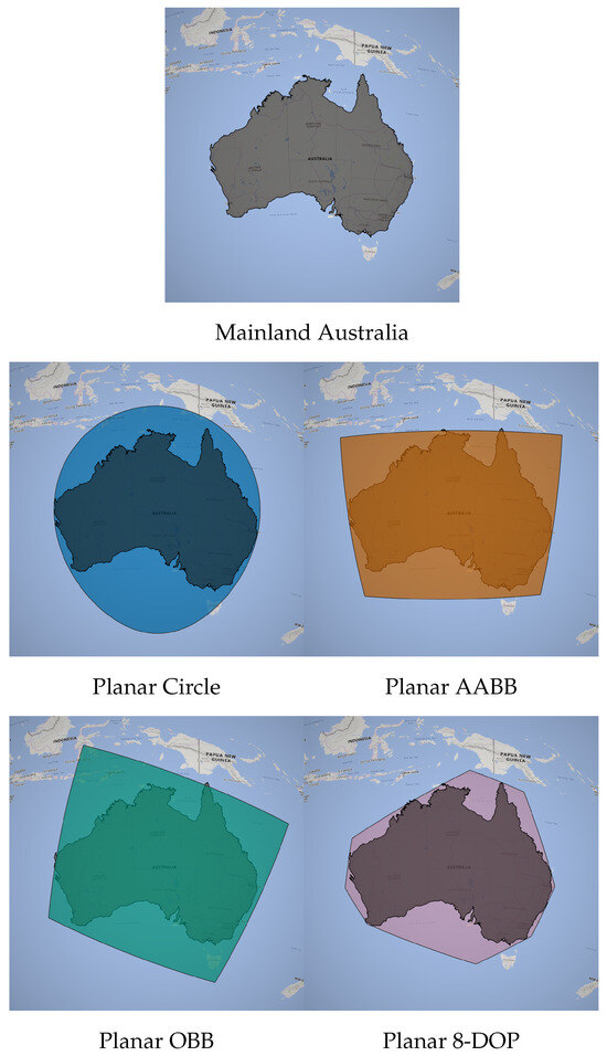
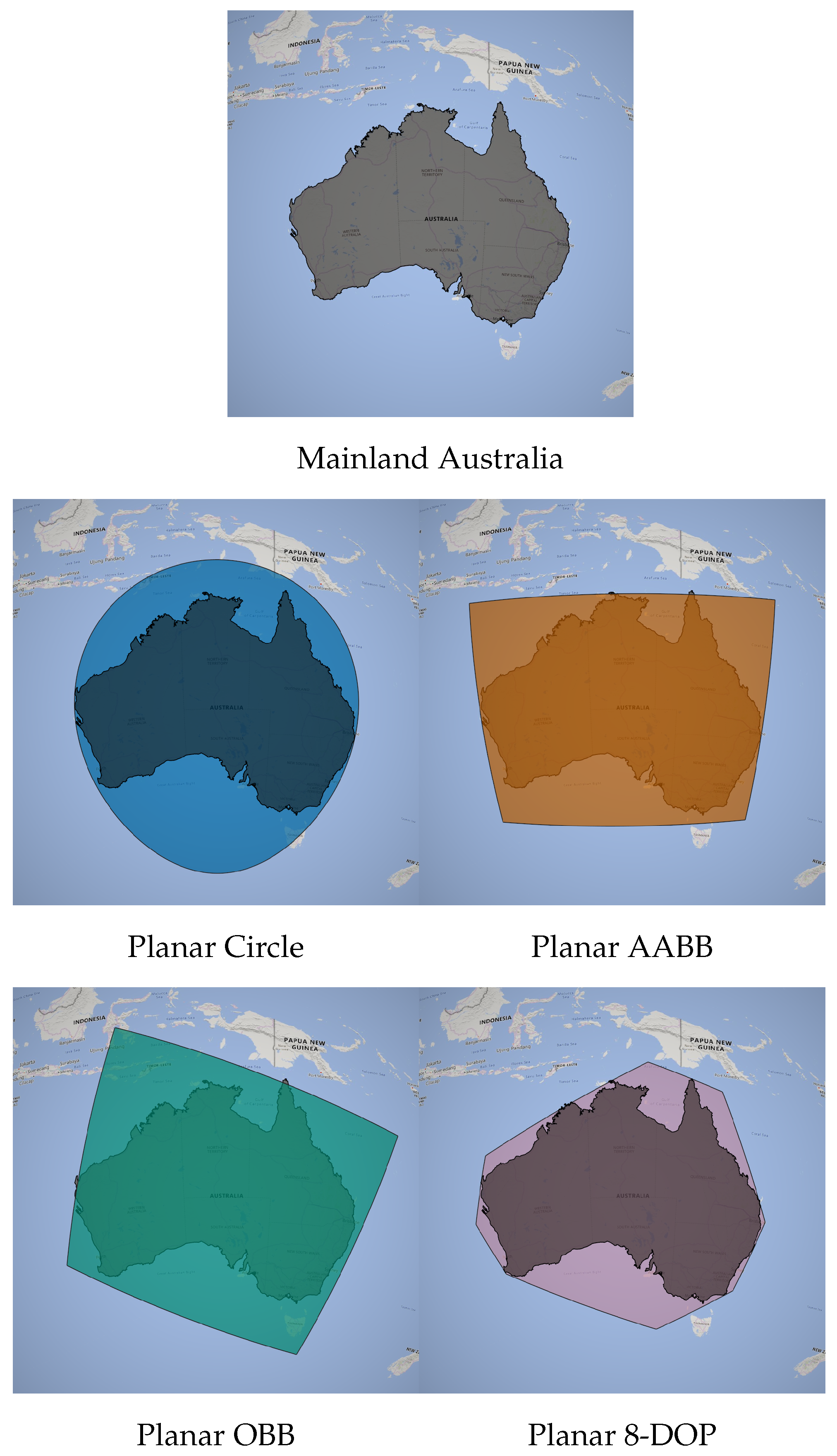
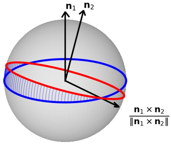
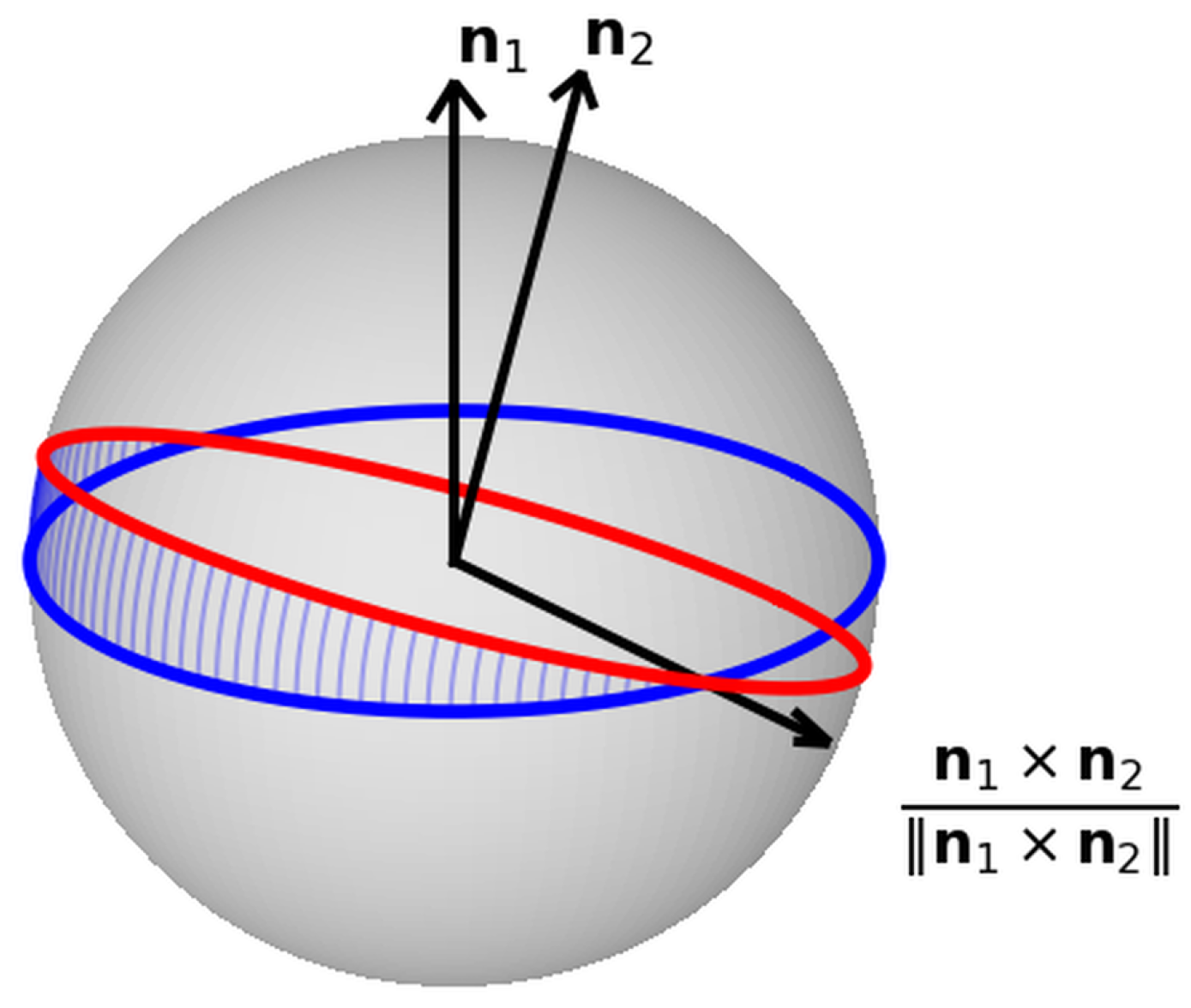
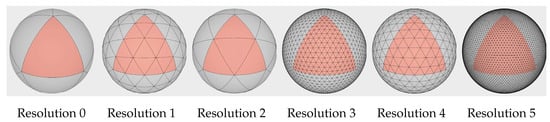
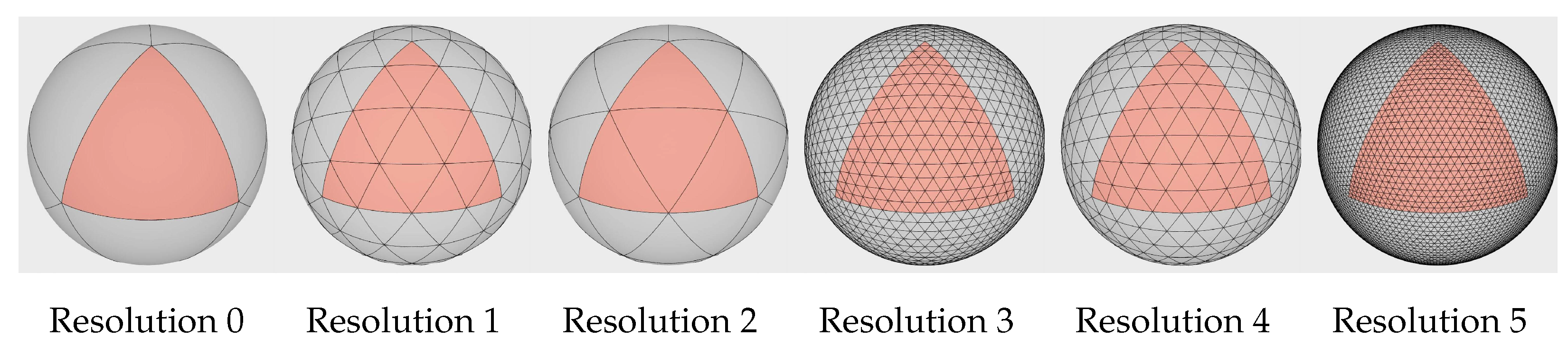
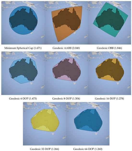
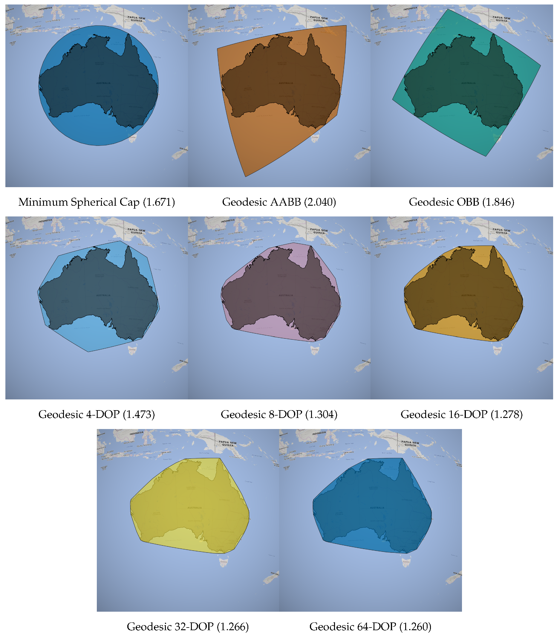
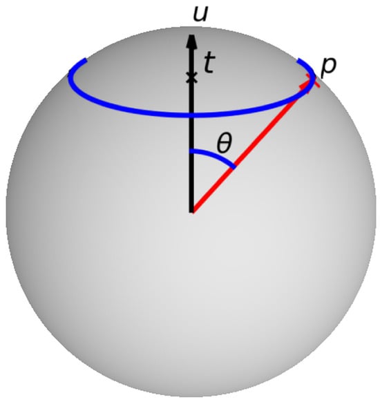
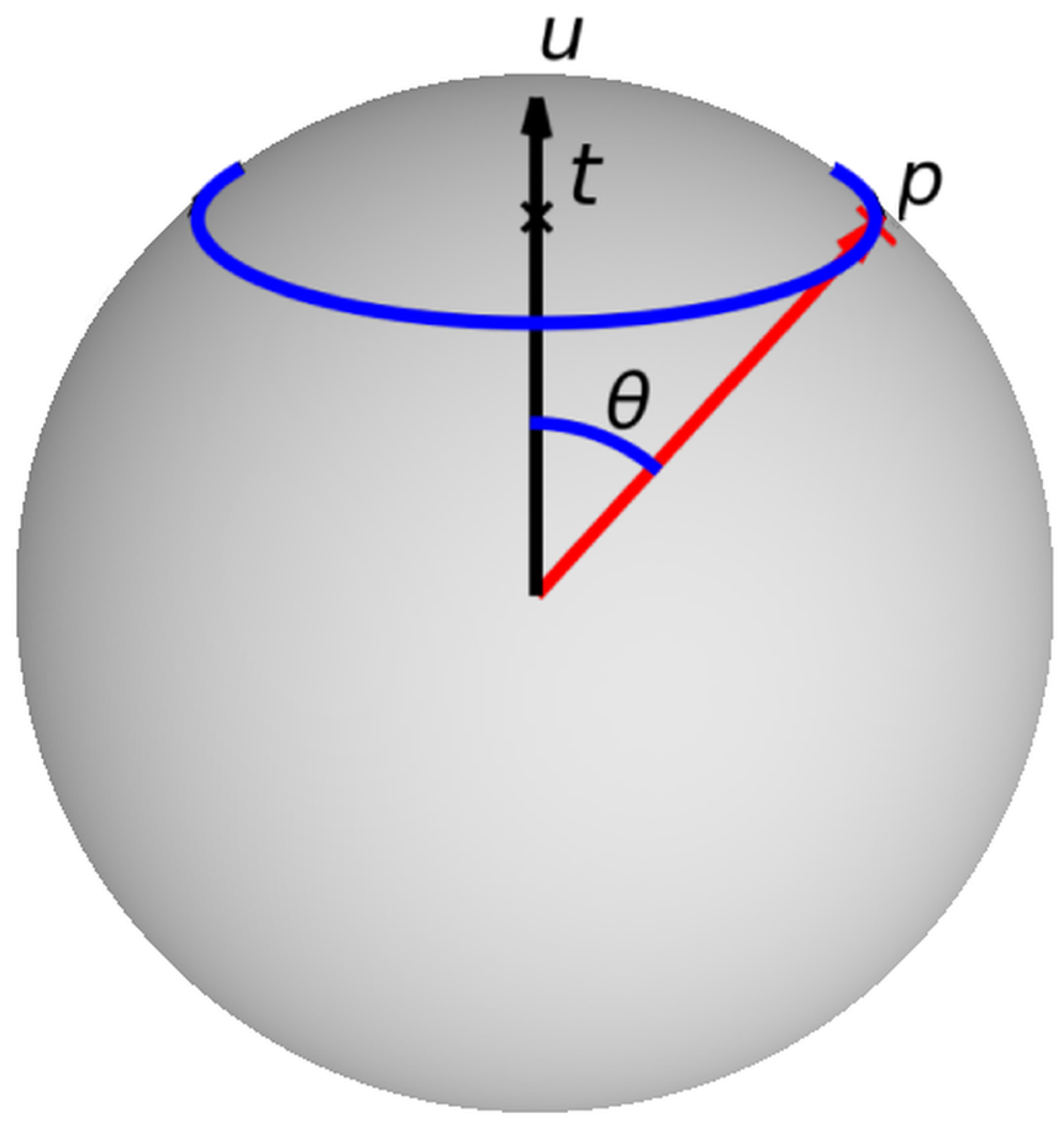
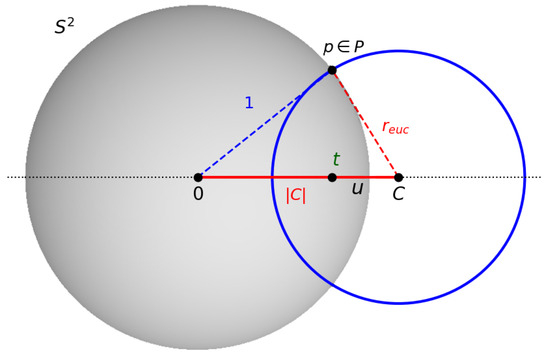
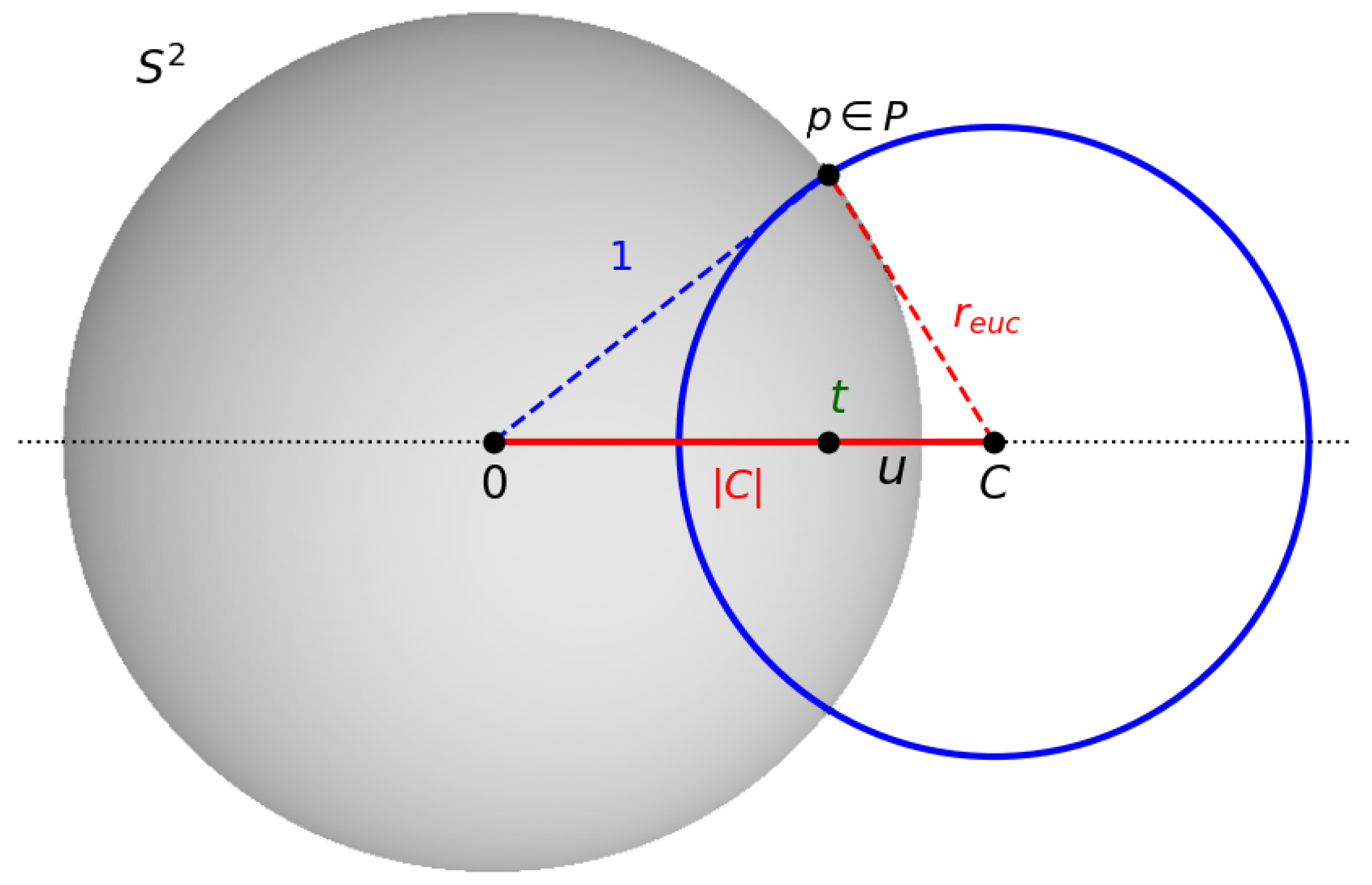
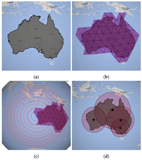
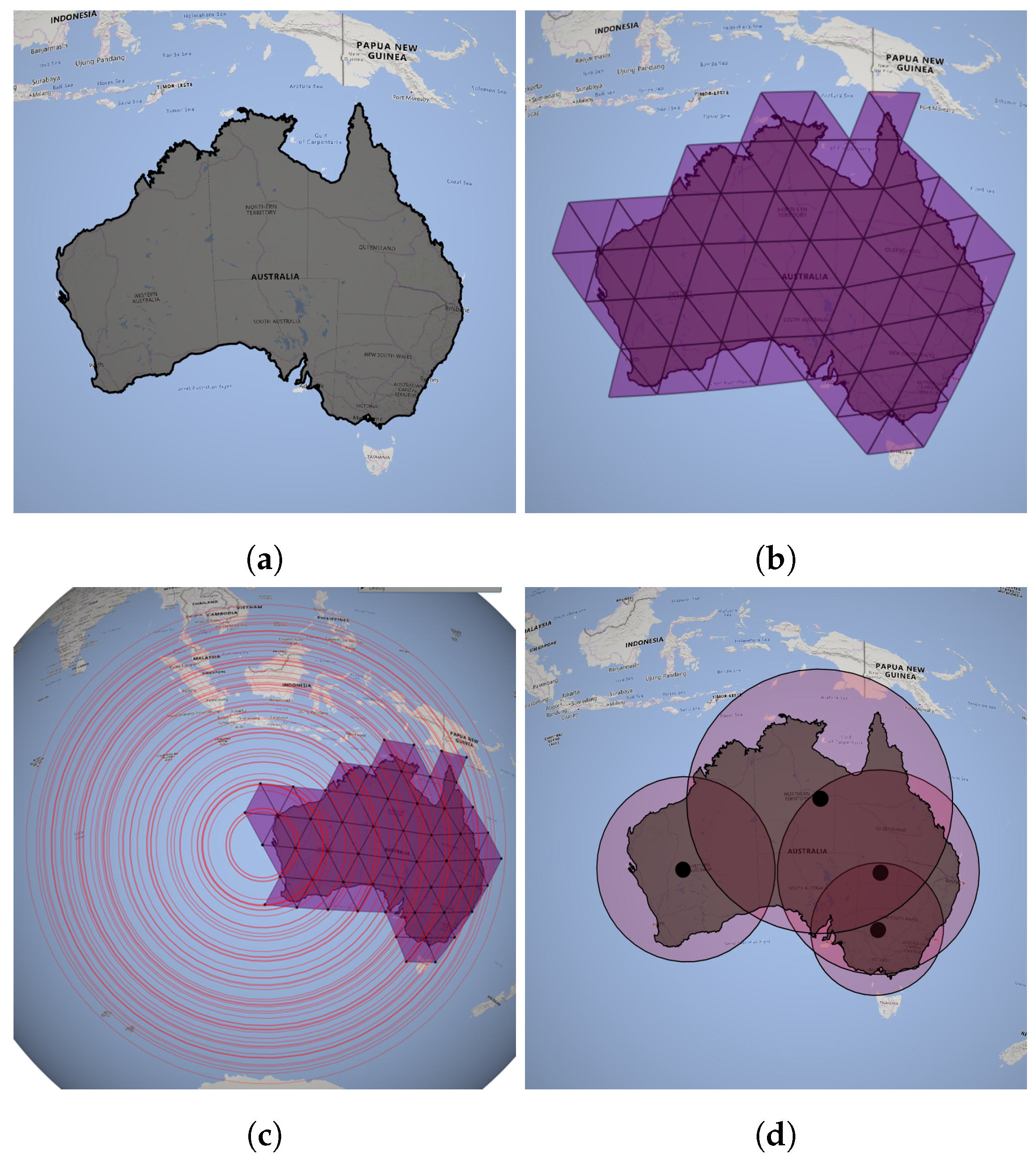
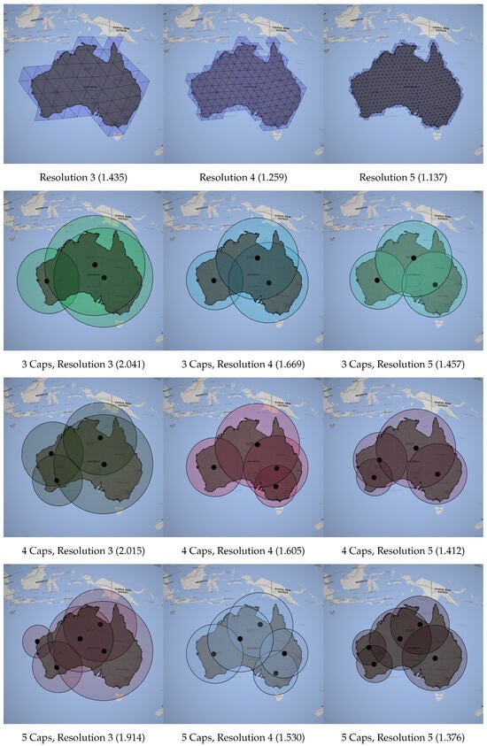
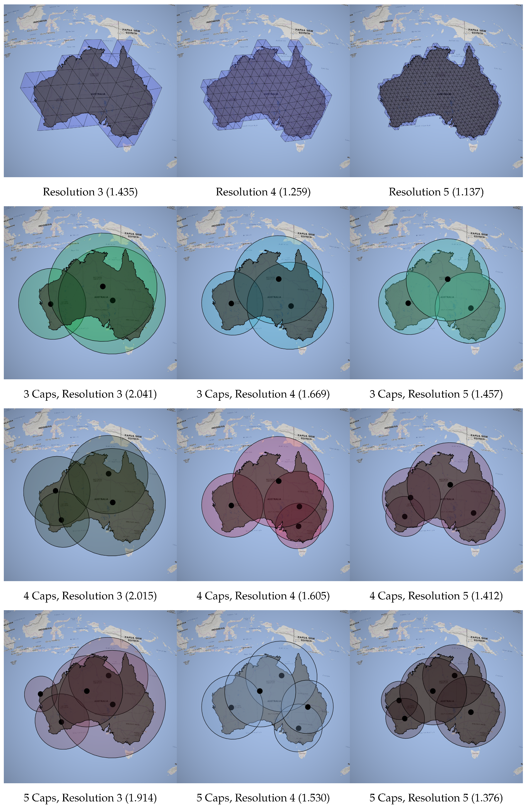
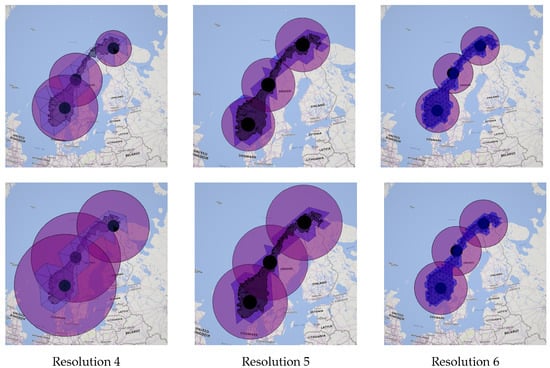
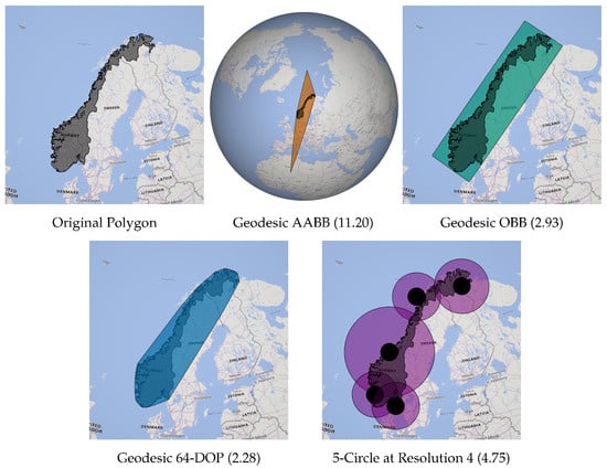

Disclaimer/Publisher’s Note: The statements, opinions and data contained in all publications are solely those of the individual author(s) and contributor(s) and not of MDPI and/or the editor(s). MDPI and/or the editor(s) disclaim responsibility for any injury to people or property resulting from any ideas, methods, instructions or products referred to in the content. |
© 2026 by the authors. Published by MDPI on behalf of the International Society for Photogrammetry and Remote Sensing. Licensee MDPI, Basel, Switzerland. This article is an open access article distributed under the terms and conditions of the Creative Commons Attribution (CC BY) license.