Two-Hourly Urban Vitality Dynamics and Spatiotemporal Heterogeneity of Built-Environment–Vitality Associations at the Parcel Scale: Evidence from Zhengzhou, China

Abstract

Urban vitality varies systematically within the day, yet its time-specific associations with stable built-environment conditions remain insufficiently understood at fine spatial scales. This study examines two-hourly urban vitality in central Zhengzhou, China, using Baidu Heatmap-derived activity intensity and multi-source built-environment data at the parcel scale. Twelve two-hourly MGWR models form the primary analysis, identifying temporal changes in the direction, magnitude, and spatial distribution of local associations. A daily mean MGWR model with the same independent variables serves as an aggregate benchmark. Results show that: (1) vitality exhibited a clear daily pulse while retaining a persistent center–corridor–node structure, with Global Moran’s I ranging from 0.508 to 0.562; (2) the two-hourly MGWR models explained 69.1–81.8% of spatial variation, compared with 39.2–66.1% for OLS, while the daily mean MGWR achieved an R² of 0.791; and (3) relative to the benchmark, the two-hourly coefficient distributions revealed variable-specific association windows, directional transitions, and changing local dispersion across transportation, land-use, and facility variables. These findings establish the added interpretive value of two-hourly analysis, support time-sensitive management, and provide diagnostic evidence on how observed daily activity patterns are distributed in relation to stable urban configurations.

1. Introduction

Urban vitality captures the spatial concentration and temporal variation in population activity within urban areas. It provides a lens for examining how activity observed at different times is distributed in relation to relatively stable spatial form, infrastructure, and urban functions. A central question for urban geography and urban management is therefore how vitality varies within the day and how its local statistical associations with built-environment conditions differ across locations and periods. At the operational scale, identifying the periods and areas in which these associations become pronounced or spatially differentiated can guide period-specific monitoring and contextual diagnosis. At the planning scale, comparing these time-specific profiles with a daily mean benchmark adds a temporal evaluation of fixed transport, land-use, and facility configurations by distinguishing associations that remain broadly sustained from those concentrated in particular periods of the daily cycle [1,2,3,4,5].

Location-aware technologies and multi-source urban sensing data have reshaped the measurement of urban vitality. Mobile positioning records, smart-card data, social media traces, trajectory data, nighttime light imagery, and other human-activity datasets make it possible to observe population activity at finer temporal intervals and spatial units [6,7,8]. These data extend vitality measurement from aggregate population or land-use proxies to dynamic evidence of urban activity, supporting the analysis of daily rhythms, activity transitions, and time-sensitive spatial processes. As a result, urban vitality research has increasingly incorporated dynamic monitoring and spatiotemporally differentiated analysis [9,10].

Existing studies have provided important evidence on the spatial distribution and built-environment–vitality associations of urban vitality. Common indicators include population activity intensity, POI density, land-use mix, nighttime light intensity, and mobile positioning data [11,12]. Previous findings show that urban vitality often displays significant spatial clustering, with high-vitality areas concentrated in urban centers, commercial districts, transport hubs, and mixed-use areas [13,14,15]. These studies have established a solid empirical basis for identifying where vitality is concentrated and how it corresponds to urban functional structure.

The built environment has been widely recognized as a set of relatively stable spatial conditions associated with urban vitality. Transportation networks support mobility and activity agglomeration through connectivity and accessibility; land-use structure defines the functional capacity of different urban spaces; and service facilities support consumption, employment, and daily life activities [16,17,18,19,20,21]. Recent research has also expanded the understanding of built-environment heterogeneity by incorporating spatial morphology and architectural complexity [17]. With the development of spatial statistical models, GWR and MGWR have been increasingly used to reveal spatial non-stationarity and scale differences in built-environment–vitality associations [22,23,24]. These approaches have advanced the analysis of how built-environment–vitality associations vary across urban space.

A finer intra-day perspective is necessary because urban vitality involves both the spatial concentration of population activity and its temporal variation across urban space. Existing studies have demonstrated differences among functional areas and across day–night or other broad temporal divisions, while many analyses continue to rely on daily aggregates or a limited number of temporal categories [2,25,26]. These approaches establish the overall relationship between built-environment characteristics and urban vitality, whereas two-hourly analysis can identify when a local association becomes pronounced, how long it persists, whether its direction changes, and how its spatial distribution varies within the day. A daily mean benchmark provides the aggregate reference required to evaluate this added temporal information under the same spatial units, explanatory variables, and modeling framework. Because roads, metro stations, land-use proportions, and facility densities retain stable measured values within the daily cycle, temporal variation in their local regression coefficients represents changes in their statistical association with time-specific population-activity distributions. This distinction connects the stable spatial organization of the city with successive time-specific population-activity distributions.

Zhengzhou provides a suitable case for examining these spatiotemporal relationships. As a national central city and the core city of the Central Plains Urban Agglomeration, Zhengzhou has experienced rapid population growth, rail transit expansion, and continuous spatial restructuring in recent years [27,28]. Its transition from a monocentric to a more polycentric urban structure has intensified the redistribution of population activities across central areas, transportation corridors, and emerging functional nodes. These characteristics make Zhengzhou suitable for examining two-hourly urban vitality dynamics and the time-conditioned spatial associations between relatively stable built-environment characteristics and population activity.

Against this background, this study uses Baidu Heatmap-derived vitality measures and multi-source built-environment data, including POIs, road networks, land use, and metro stations, to examine two-hourly urban vitality dynamics at the parcel scale. The analytical core consists of twelve MGWR models fitted to successive two-hourly vitality outcomes over a complete daily cycle. A daily mean vitality outcome is incorporated within the same analytical workflow as an aggregate benchmark, allowing the temporal information revealed by the time-specific coefficients to be interpreted relative to an overall association level. Here, the parcel scale refers to road-bounded urban blocks, which preserve relatively coherent morphological and functional spaces and support fine-grained correspondence between built-environment conditions and population activity. Specifically, this study aims to:

① Characterize the two-hourly evolution of parcel-level urban vitality over a complete daily cycle, distinguishing its persistent spatial organization from intra-day changes in activity intensity and spatial clustering;

② With the built-environment variables held constant across all time slices, identify when and where their local MGWR coefficients strengthen, weaken, or change direction, and examine the corresponding changes in coefficient magnitude, spatial extent, and local dispersion;

③ Evaluate the temporal and local information added by the twelve two-hourly models relative to a daily mean MGWR benchmark, focusing on variable-specific association windows, directional transitions, and changes in spatial extent and local dispersion.

The specific analytical contribution of this study lies in resolving an aggregate built-environment–vitality relationship into twelve parcel-scale local coefficient surfaces observed at two-hour intervals. With the spatial units, explanatory variables, and modeling framework held constant, the daily mean MGWR provides an aggregate reference for identifying the information added by temporal disaggregation. This design reveals variable-specific association windows, directional transitions, changes in spatial extent, and time-varying local dispersion across the sampled daily cycle.

2. Materials and Methods

2.1. Study Area

Zhengzhou is located in the north-central part of Henan Province and serves as a national central city, the core city of the Central Plains Urban Agglomeration, and a major national transportation hub. In recent years, continuous urbanization, the rapid expansion of the rail transit network, and sustained population growth have led to substantial changes in the city’s spatial structure and urban vitality patterns. As a result, Zhengzhou has exhibited a typical transition from a monocentric to a polycentric urban structure. Meanwhile, urban vitality exhibits pronounced spatiotemporal dynamics, making Zhengzhou an ideal case for investigating the spatiotemporal variation in urban vitality and its associations with the built environment (Figure 1).

Figure 1. Location of the study area and parcel units in Zhengzhou. (a) Location of Henan Province; (b) location of Zhengzhou; and (c) the study area and 2663 parcel units within the Fourth Ring Road. Parcel units were delineated based on roads, railways, rivers, green spaces, and other morphological boundaries.

Figure 1. Location of the study area and parcel units in Zhengzhou. (a) Location of Henan Province; (b) location of Zhengzhou; and (c) the study area and 2663 parcel units within the Fourth Ring Road. Parcel units were delineated based on roads, railways, rivers, green spaces, and other morphological boundaries.

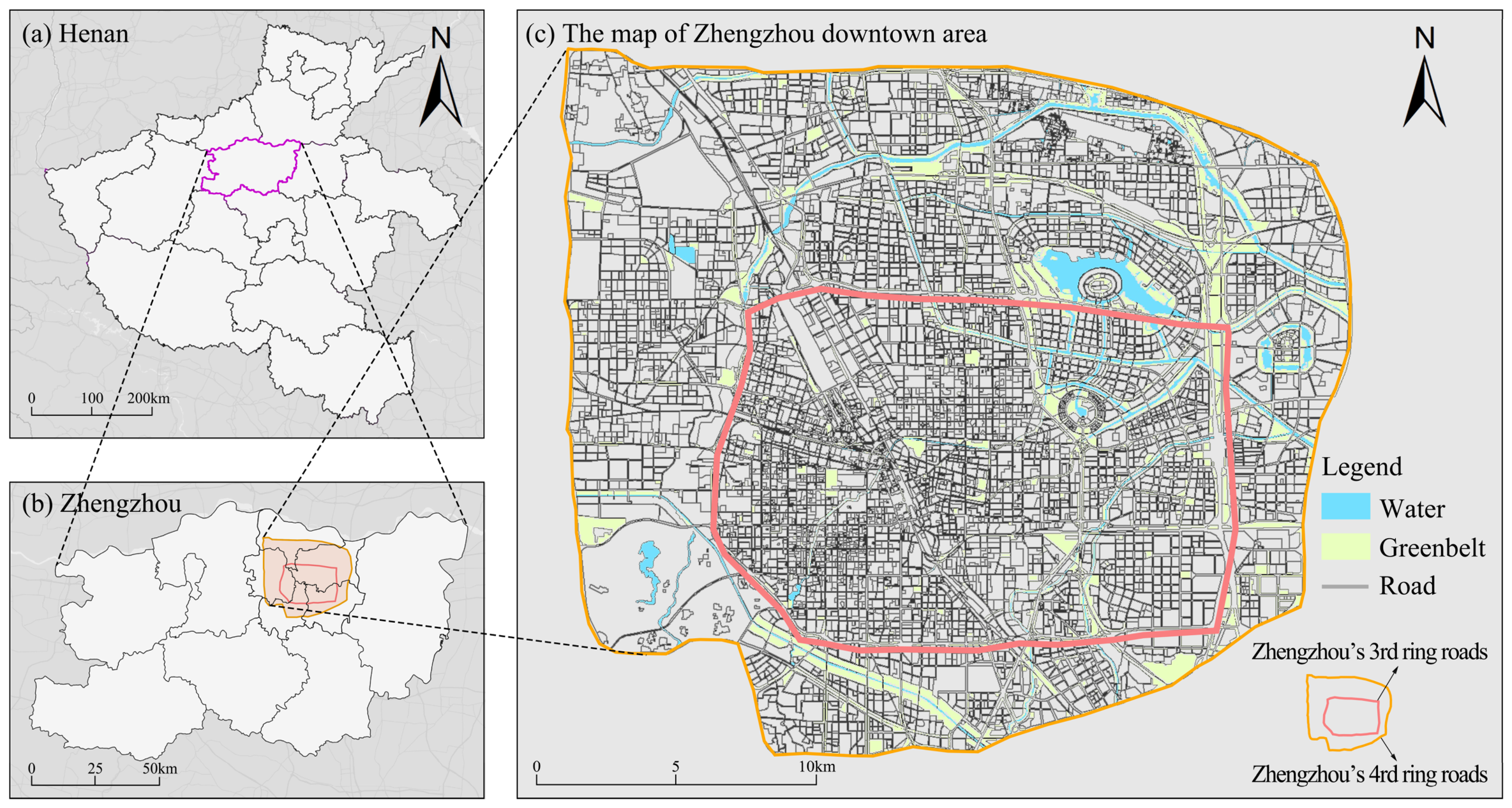
Given that the central urban area concentrates Zhengzhou’s major commercial centers, transportation hubs, and population activity zones, it effectively reflects the spatial organization of urban vitality. Therefore, the area within the Fourth Ring Road was selected as the study area. Based on road network characteristics and urban spatial morphology, a total of 2663 parcel units were delineated through visual interpretation of remote sensing imagery and used as the basic analytical units. Parcel boundaries were manually delineated from high-resolution remote-sensing imagery using roads, railways, rivers, green spaces, and other identifiable morphological features, and were cross-checked against road-network data and online basemaps. Compared with regular grids or larger administrative units, parcels better preserve coherent functional and morphological spaces and more closely reflect the spatial organization of the built environment and everyday activity. Although parcel delineation followed consistent morphological criteria and was cross-checked using multiple spatial data sources, some interpreter-dependent judgment may remain where morphological boundaries are ambiguous. Therefore, minor differences in parcel boundaries may arise across independent interpreters, representing a potential limitation in the reproducibility of the parcel-construction process.

2.2. Methodological Framework

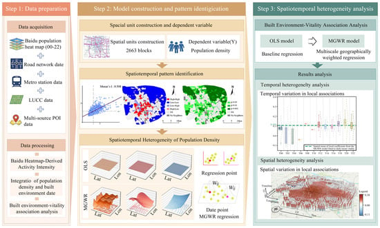
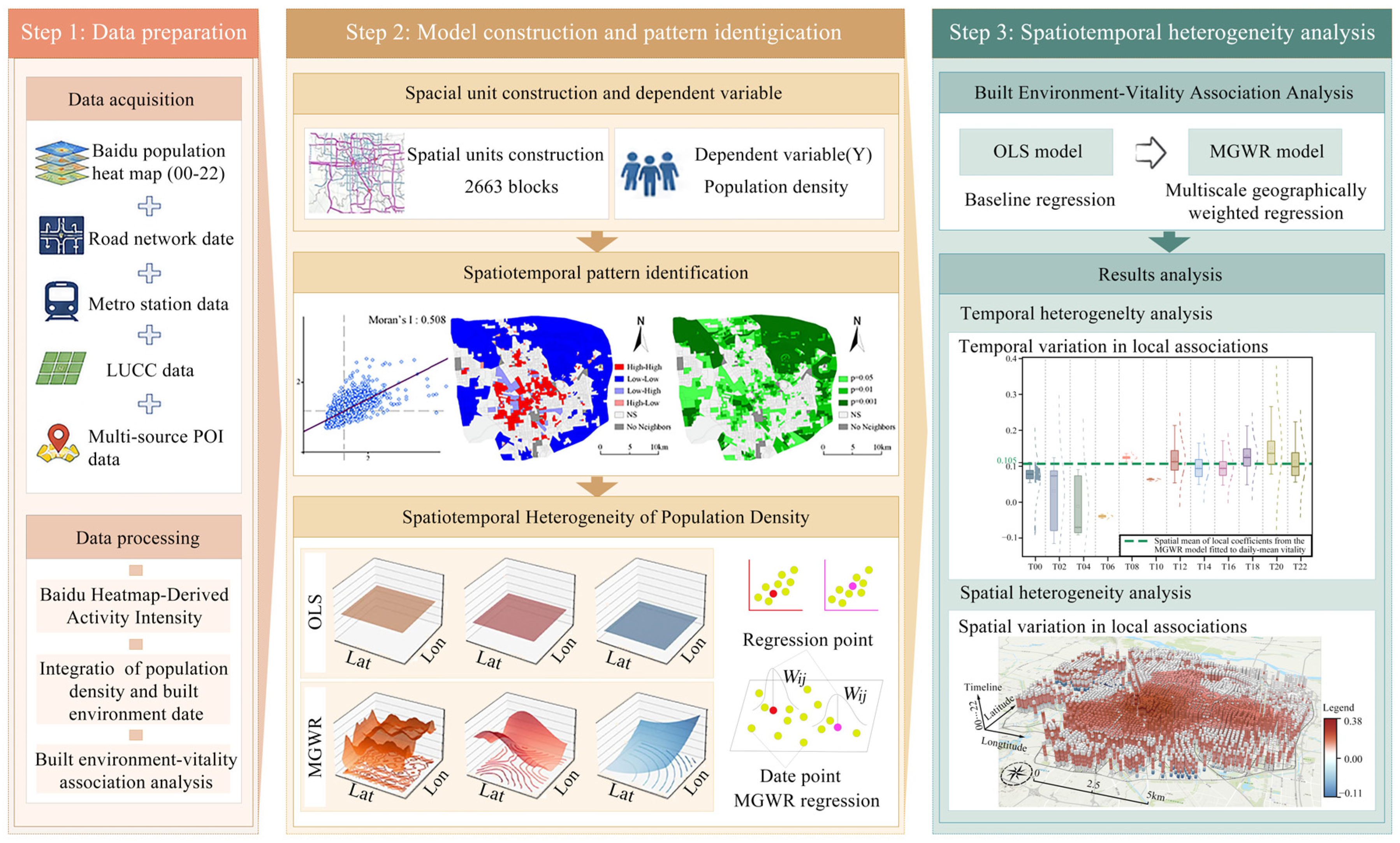
This study developed a methodological framework centered on the identification and interpretation of two-hourly urban-vitality dynamics. First, population-activity intensity at twelve two-hourly time slices was extracted from Baidu Heatmap data and integrated with road-network, rail-transit, land-use, and POI data to construct a parcel-scale database. A daily mean vitality surface was simultaneously derived from the twelve time-specific vitality values to provide an aggregate benchmark. Second, spatial-distribution and spatial-autocorrelation analyses were used to characterize the persistence and temporal variation in urban-vitality patterns. Third, twelve time-specific MGWR models were calibrated as the primary models for estimating local built-environment–vitality associations. OLS and GWR provided global and spatial model references, while GTWR assessed continuity across adjacent periods. The daily mean MGWR was used to establish the aggregate coefficient reference for interpreting the time-specific results. Finally, the two-hourly coefficient distributions were evaluated relative to this benchmark, and space–time cubes were used to identify their temporal persistence and spatial expression. All coefficients were interpreted as local statistical associations. The overall methodological framework is illustrated in Figure 2.

Figure 2. Methodological framework. The workflow includes data acquisition and preprocessing, identification of spatiotemporal patterns of urban vitality, spatial autocorrelation analysis, MGWR modeling, and spatiotemporal heterogeneity analysis of built-environment–vitality associations.

2.3. Data Sources and Preprocessing

2.3.1. Urban Vitality Data and Daily Mean Benchmark Construction

Urban vitality data were obtained from the Baidu Heatmap platform, which provides a location-based proxy for population activity intensity and spatial distribution. To reduce the influence of single-day fluctuations, heatmap data were collected on ten dates in 2025: 15 January, 17 January, 19 January, 20 January, 21 January, 3 February, 5 February, 7 February, 9 February, and 11 February. For each date, data were collected at twelve two-hourly time slices: 00:00, 02:00, 04:00, 06:00, 08:00, 10:00, 12:00, 14:00, 16:00, 18:00, 20:00, and 22:00.

The twelve time slices represent a complete 24 h daily cycle. The 22:00 observation represents the final period extending toward 24:00, while 24:00 corresponds to 00:00 of the following daily cycle. For each time slice, heatmap values from the ten sampled dates were averaged. The resulting raster surface was overlaid with the parcel units, and the mean pixel value within each parcel was calculated as its time-specific urban vitality value, V_it. These twelve parcel-level surfaces constitute the dependent variables of the primary two-hourly analysis. Within the same data-processing procedure, daily mean vitality was calculated for each parcel as ${\overline{V}}_i={\displaystyle \frac{1}{12}}{\sum }_{t=1}^{12}{V}_{it}$. This daily mean outcome was used solely to establish the aggregate benchmark. Thus, the averaging operation was applied to the vitality outcome before regression, and the coefficients of the daily mean model were generated by fitting MGWR to this aggregated dependent variable.

2.3.2. Built-Environment Data

The built-environment data used in this study include road network data, land-use data, and multi-source POI data.

Road network data were used to calculate road betweenness and road network integration. Metro-station data were employed to derive the indicator of distance to the nearest metro station. Land-use data were used to extract the residential land percentage and commercial land percentage. Based on their functional attributes, POI data were classified into four categories: catering POIs, enterprise POIs, shopping service POIs, and life service facility POIs, for which kernel density values were calculated separately.

All datasets were projected into a unified coordinate system. Spatial overlay analysis was then performed to obtain the corresponding indicator values for each parcel unit, thereby constructing the built-environment database used in subsequent analyses (Table 1).

Table 1. Data sources and descriptions.

Data Type	Original Source	Acquisition or Extraction Method	Derived Data
Administrative boundary data	Planning Cloud (Guihuayun)	Downloaded and clipped to the study area	Study-area boundary
Remote-sensing imagery	Google Maps * satellite imagery and Baidu Maps basemap	Manual visual interpretation and cross-checking using identifiable roads, railways, rivers, green spaces, and other morphological boundaries	Parcel boundaries, road network, and land-use polygons
Population Activity Data	Baidu Heatmap *, based on location-based service (LBS) data	Collected at 12 two-hourly time slices on 10 sampling dates; averaged by time slice and aggregated to parcels using mean pixel values	Twelve parcel-level two-hourly vitality surfaces and one daily mean benchmark surface
POI Data	Amap Open Platform * (Gaode Map)	Data cleaning, functional reclassification, and kernel-density estimation	Kernel densities of catering, enterprise, shopping-service, and life-service POIs

* Baidu Heatmap and Amap are widely used location-based data platforms in China, providing population-activity intensity and geocoded POI information, respectively. Google Maps satellite imagery and Baidu Maps basemaps were used as reference sources for manual interpretation of parcels, road networks, and land use. Comparable datasets in other regions may be obtained from mobile-phone positioning data, social-media records, business directories, or other location-based services, although their characteristics may differ.

Table 1. Data sources and descriptions.

Data Type	Original Source	Acquisition or Extraction Method	Derived Data
Administrative boundary data	Planning Cloud (Guihuayun)	Downloaded and clipped to the study area	Study-area boundary
Remote-sensing imagery	Google Maps * satellite imagery and Baidu Maps basemap	Manual visual interpretation and cross-checking using identifiable roads, railways, rivers, green spaces, and other morphological boundaries	Parcel boundaries, road network, and land-use polygons
Population Activity Data	Baidu Heatmap *, based on location-based service (LBS) data	Collected at 12 two-hourly time slices on 10 sampling dates; averaged by time slice and aggregated to parcels using mean pixel values	Twelve parcel-level two-hourly vitality surfaces and one daily mean benchmark surface
POI Data	Amap Open Platform * (Gaode Map)	Data cleaning, functional reclassification, and kernel-density estimation	Kernel densities of catering, enterprise, shopping-service, and life-service POIs

* Baidu Heatmap and Amap are widely used location-based data platforms in China, providing population-activity intensity and geocoded POI information, respectively. Google Maps satellite imagery and Baidu Maps basemaps were used as reference sources for manual interpretation of parcels, road networks, and land use. Comparable datasets in other regions may be obtained from mobile-phone positioning data, social-media records, business directories, or other location-based services, although their characteristics may differ.

2.4. Built-Environment Variables

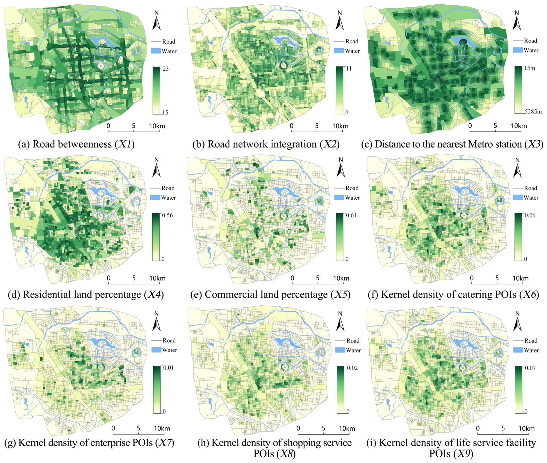
Built-environment variables were organized into three dimensions: transport-related spatial conditions, land-use composition, and facility configuration. Nine explanatory variables were included (Figure 3).

(1)

Transport-related spatial conditions. Road betweenness (X1) represents topological through-movement potential within the fixed road network, road-network integration (X2) represents topological connectedness within that network, and distance to the nearest metro station (X3) represents spatial proximity to rail transit. These indicators characterize network structure and station proximity rather than observed traffic flows, modal choices, or time-specific station use.

(2)

Land-use composition. Residential land percentage (X4) and commercial land percentage (X5) measure the respective shares of parcel area occupied by residential and commercial land.

(3)

Facility configuration. Kernel densities of catering POIs (X6), enterprise POIs (X7), shopping-service POIs (X8), and life-service POIs (X9) represent the spatial concentrations of the four measured facility categories.

The three transport-related indicators cover part of the multimodal accessibility environment. Temporally consistent data on bus services, pedestrian networks, cycling conditions, and observed traffic flows were unavailable for the study period; these dimensions are addressed as limitations in Section 4.4.

The built-environment variable system adopted in this study is presented in Table 2.

Table 2. Built-environment variables and definitions.

Type	Variable	Variable Name	Description
Transport-related spatial conditions	X1	Road betweenness	Topological through-movement potential within the fixed road network, derived from space syntax
	X2	Road network integration	Topological connectedness within the fixed road network, derived from space syntax
	X3	Distance to the nearest metro station	Spatial proximity to rail transit, measured by distance to the nearest metro station
Land-use composition	X4	Residential land percentage	Share of parcel area occupied by residential land
	X5	Commercial land percentage	Share of parcel area occupied by commercial land
Facility configuration	X6	Kernel density of catering POIs	Spatial concentration of catering POIs
	X7	Kernel density of enterprise POIs	Spatial concentration of enterprise POIs
	X8	Kernel density of shopping service POIs	Spatial concentration of shopping-service POIs
	X9	Kernel density of life service facility POIs	Spatial concentration of life-service POIs

Figure 3. Spatial distribution of the nine built-environment variables. (a) Road betweenness; (b) road network integration; (c) distance to the nearest metro station; (d) residential land percentage; (e) commercial land percentage; (f) kernel density of catering POIs; (g) kernel density of enterprise POIs; (h) kernel density of shopping service POIs; (i) kernel density of life service facility POIs.

Figure 3. Spatial distribution of the nine built-environment variables. (a) Road betweenness; (b) road network integration; (c) distance to the nearest metro station; (d) residential land percentage; (e) commercial land percentage; (f) kernel density of catering POIs; (g) kernel density of enterprise POIs; (h) kernel density of shopping service POIs; (i) kernel density of life service facility POIs.

2.5. Spatial Analysis Methods

2.5.1. Spatial Autocorrelation Analysis

Spatial analysis methods were employed to identify the spatial patterns and clustering characteristics of urban vitality. Specifically, Global Moran’s I [29] and Local Moran’s I (LISA) [30] were used to examine the spatial autocorrelation of urban vitality.

Global Moran’s I measures the overall degree of spatial autocorrelation and is used to evaluate whether the spatial distribution of urban vitality exhibits significant clustering, dispersion, or randomness across the study area [31]. The formula is expressed as follows:

$$GlobalMoran’sI={\displaystyle \frac{n{\displaystyle {\sum }_{i=1}^n}{\displaystyle {\sum }_{j\ne i}^n}{w}_{ij}\left(X_i-\overline{X}\right)\left(X_j-\overline{X}\right)}{{\displaystyle {\sum }_{i=1}^n}{\displaystyle {\sum }_{j\ne i}^n}{w}_{ij}{{\displaystyle {\sum }_{i=1}^n}\left(X_i-\overline{X}\right)}^2}}$$

(1)

where n is the number of observations; Wij denotes the spatial weight between spatial units i and j; X_i and X_j represent the values of the variable for parcels i and j, respectively, which, in this study, correspond to urban vitality values represented by population density at different time periods; and $\overline{X}$ is the mean value of all observations. A Queen contiguity-based spatial weights matrix (W) was constructed based on parcel adjacency, with parcels sharing either a common boundary or a vertex defined as spatial neighbors. The same spatial weighting scheme was applied to both Global Moran’s I and LISA analyses. The value of Global Moran’s I ranges were [−1, 1]. A positive value indicates positive spatial autocorrelation, suggesting a clustered spatial distribution pattern, with larger values representing stronger spatial clustering. Conversely, a negative value indicates negative spatial autocorrelation, implying a dispersed spatial distribution pattern.

Global Moran’s I cannot identify the spatial correlation and heterogeneity between individual spatial units and their neighboring units. To address this limitation, Local Moran’s I (LISA) is employed to detect local spatial autocorrelation and identify localized clustering patterns. Therefore, Local Moran’s I is commonly used in conjunction with Global Moran’s I. Its calculation is expressed as follows [32]:

$$I_{LISA}={\displaystyle \frac{\left(X_i-\overline{X}\right)}{{{\displaystyle {\sum }_{i=1}^n}\left(X_i-\overline{X}\right)}^2}}{\displaystyle \sum _{j=1}^n}{W}_{ij}\left(X_j-\overline{X}\right)$$

(2)

A positive value of I_LISA indicates positive local spatial autocorrelation, whereas a negative value indicates negative local spatial autocorrelation. Based on the significance and spatial association patterns, LISA cluster maps can be classified into four types: ① High–High (H–H) cluster: I_LISA > 0, where both parcel i and its neighboring parcels have urban vitality values above the mean. ② Low–Low (L–L) cluster: I_LISA > 0, where both parcel i and its neighboring parcels have urban vitality values below the mean. ③ High–Low (H–L) outlier: I_LISA < 0, where parcel i has an urban vitality value above the mean, while its neighboring parcels have values below the mean. ④ Low–High (L–H) outlier: I_LISA < 0, where parcel i has an urban vitality value below the mean, whereas its neighboring parcels have values above the mean.

2.5.2. Multiscale Geographically Weighted Regression (MGWR)

The Multiscale Geographically Weighted Regression (MGWR) model is an extension of the Geographically Weighted Regression (GWR) model. Both are local regression models that allow regression coefficients to vary across space. Unlike traditional global regression models, which assume that regression coefficients remain spatially constant, GWR and MGWR explicitly incorporate the spatial locations of observations into the coefficient estimation process. Consequently, spatial location becomes a key parameter in model calibration. The classical GWR model can be expressed as follows [33]:

$$y_i={\beta }_0\left(u_i,v_i\right)+{\sum }_{j=1}^k{\beta }_j\left(u_i,v_i\right)x_{ij}+{\epsilon }_i$$

(3)

In Equation (3), (u_i,v_i) denotes the geographic coordinates of the centroid of parcel i; yi represents the urban vitality represented by Baidu Heatmap-derived activity intensity of parcel i measured at a given two-hourly interval; and (xi1,xi2…xi9) denotes the vector of built-environment variables for parcel i. βi0 and ε_i represent the intercept and random error term for parcel i, respectively. (βi1(ui,vi), βi2(ui,vi) … βi9(ui,vi)) is the vector of local regression coefficients to be estimated for parcel i, which can be estimated as follows:

$$\widehat{\beta }\left(u_i,v_i\right)={\left[X^{T}W\left(u_i,v_i\right)X\right]}^{-1}{X}^{T}W\left(u_i,v_i\right)y$$

(4)

where W(u_i,v_i) is the spatial weighting matrix.

As an extension of the GWR model, the MGWR model allows the relationships between explanatory variables and the dependent variable to vary across different spatial scales. In MGWR, the optimal bandwidth for each variable is determined through spatial search, thereby reducing potential mismatches between bandwidth selection and parameter estimation for specific samples. This enables a more accurate understanding of the scale effects and spatial variation patterns of spatial variation in built-environment–vitality associations across different time periods. The model is expressed as follows:

$$y_i={\beta }_{bw0}\left(u_i,{\mathrm{v}}_i\right)+{\displaystyle \sum _{j=1}^k}{\beta }_{bwj}\left(u_i,{\mathrm{v}}_i\right)x_{ij}+{\epsilon }_i$$

(5)

In Equation (5), b_w0 denotes the bandwidth associated with the intercept, while b_wj denotes the variable-specific optimal spatial bandwidth for the jth explanatory variable. The term β_bwj(u_i, v_i) represents the local coefficient estimated for the jth explanatory variable at parcel i using bandwidth b_wj.

The MGWR model was implemented using mgwr-2.2.1 (https://sgsup.asu.edu/sparc/multiscale-gwr (accessed on 17 January 2025)).

3. Results

3.1. Two-Hourly Dynamics of Urban Vitality

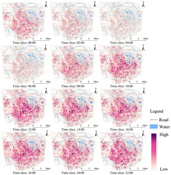
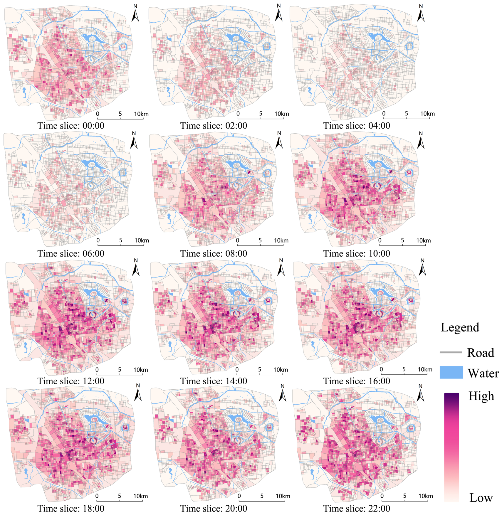
Urban vitality in Zhengzhou exhibited marked intra-day variation within a persistent center–corridor–node spatial structure (Figure 4). Across the twelve time slices, high-vitality parcels remained concentrated in the central urban area, along major transport corridors, and around selected functional nodes, while their intensity and spatial extent varied through the day.

Figure 4. Two-hourly urban vitality distribution in Zhengzhou. The figure presents urban vitality across twelve two-hourly time slices (00:00–22:00) over a 24 h cycle. The 22:00 time slice represents the final two-hour period of the day (22:00–24:00), whereas 24:00 is not shown separately because it is equivalent to 00:00 of the following day.

From 00:00 to 06:00, high-vitality parcels occupied a relatively limited spatial extent and contracted progressively after 02:00. From 08:00 onward, high-vitality areas expanded from the central urban area toward major corridors. By 10:00, a more extensive and spatially continuous pattern had formed, which remained broadly visible through 18:00.

After 20:00, high-vitality areas became more concentrated again, although the principal urban core and several activity nodes remained visible at 22:00. The observed sequence therefore comprised early-morning contraction, daytime expansion, and evening reconcentration around a relatively stable center–corridor–node framework. These results describe changes in activity intensity and spatial distribution.

3.2. Spatial Clustering Characteristics of Urban Vitality

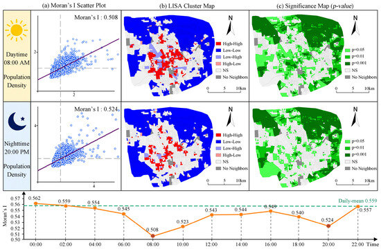
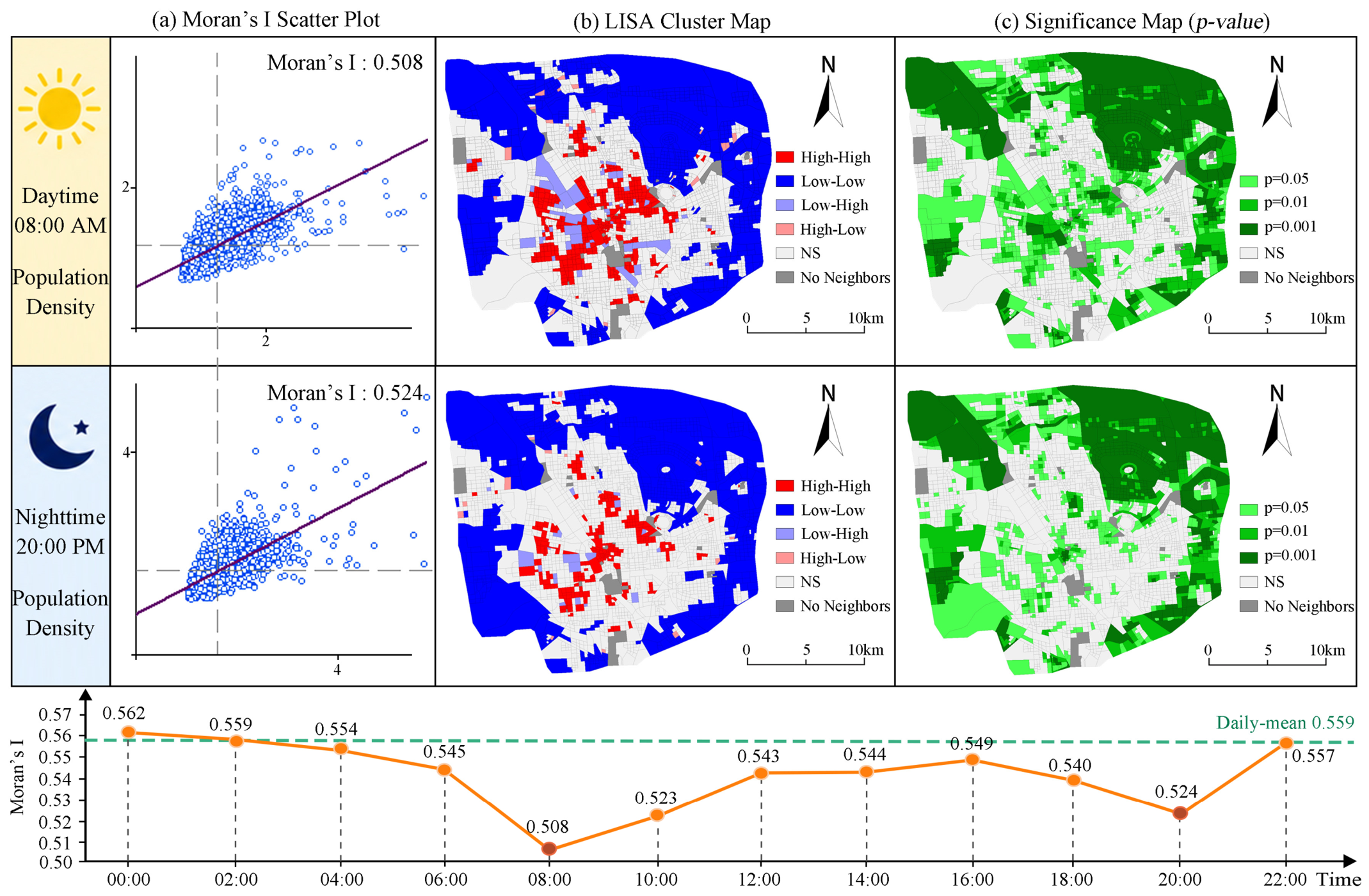
Global Moran’s I was positive at all twelve time slices, ranging from 0.508 to 0.562 and indicating persistent positive spatial autocorrelation throughout the daily cycle. The highest value occurred at 00:00 (0.562), while the lowest occurred at 08:00 (0.508); a second local trough occurred at 20:00 (0.524). These temporal values identify stage-specific changes in spatial clustering during the morning and evening transitions. The daily mean vitality surface yielded a Global Moran’s I of 0.559, close to the maximum time-specific value and higher than most two-hourly values. This benchmark summarizes the persistent aggregate clustering of urban vitality and provides a reference for interpreting the temporal fluctuations identified by the primary two-hourly analysis (Figure 5).

Figure 5. Spatial autocorrelation characteristics of urban vitality. (a) Moran’s scatter plot; (b) LISA cluster map and (c) significance map in Global Moran’s I across two-hour intervals. HH = High–High cluster; LL = Low–Low cluster; HL = High–Low outlier; LH = Low–High outlier; NS = not significant (p ≥ 0.05); the green dashed line in panel the Global Moran’s I of the daily mean urban vitality surface (0.559).

To further examine the local spatial patterns corresponding to these temporal fluctuations, Local Moran’s I (LISA) analysis was conducted for all twelve time slices. To avoid excessive and repetitive mapping, Figure 5 presents only 08:00 and 20:00 as two representative periods of relatively low spatial clustering. The 08:00 time slice corresponds to the daily minimum of Global Moran’s I, whereas 20:00 represents a local trough during the evening transition. These two periods therefore provide representative views of local clustering when overall spatial concentration was relatively weakened at different stages of the daily activity cycle. The LISA maps show clear High–High and Low–Low clusters at both time points, although their spatial distributions differed.

The Global and Local Moran’s I results jointly show that persistent citywide clustering coexisted with period-specific changes in the extent and arrangement of local clusters. The 08:00 minimum and the 20:00 local trough identify two periods in which the spatial concentration of vitality was relatively weaker within the sampled daily cycle. Their occurrence at different stages of the day demonstrates that a similar reduction in global clustering can correspond to different local spatial configurations.

3.3. Multicollinearity Diagnosis and Model Performance Comparison

Before regression analysis, Pearson’s correlation coefficients and variance inflation factors were used to assess potential multicollinearity among the explanatory variables. Particular attention was given to the correlation between road betweenness and road-network integration and among the four POI kernel-density variables. A VIF value below 5 was considered to indicate the absence of serious multicollinearity. Variables exceeding the threshold were reassessed according to their theoretical relevance, degree of correlation, and model stability. The VIF values in this article are all below 5, indicating no severe multicollinearity. Therefore, no serious multicollinearity was identified among the explanatory variables (Table 3).

Table 3. Collinearity diagnostics for the explanatory variables (VIF).

	X1	X2	X3	X4	X5	X6	X7	X8	X9
1/VIF	0.883	0.786	0.825	0.729	0.532	0.256	0.626	0.433	0.250
VIF	1.133	1.272	1.212	1.372	1.880	3.908	1.597	2.308	4.003

The model comparison was designed primarily to evaluate the suitability of spatially varying models for the twelve two-hourly vitality outcomes. OLS provides a global reference with spatially constant coefficients, GWR allows the coefficients to vary across space, and MGWR further permits variable-specific spatial bandwidths. GTWR incorporates spatial and temporal proximity and was used to assess continuity across adjacent periods. The daily mean OLS, GWR, and MGWR results were included as an aggregate benchmark for interpreting the performance of the time-specific models.

Across the twelve time slices, OLS produced R² values of 0.392–0.661, GWR produced values of 0.715–0.822, and MGWR produced values of 0.691–0.818 (Table 4). The local regression models therefore explained a larger proportion of the time-specific spatial variation than OLS. GWR and MGWR showed broadly comparable explanatory performance, while MGWR consistently produced lower AICc values and allowed the association of each explanatory variable to be estimated at its own spatial scale. These properties supported the use of MGWR for the subsequent two-hourly coefficient analysis.

Table 4. Model performance for the twelve two-hourly vitality outcomes and the daily mean benchmark.

Time	OLS			GWR			MGWR			GTWR *
	AICc	R2	Adj. R2	AICc	R2	Adj. R2	AICc	R2	Adj. R2	AICc	R2	Adj. R2
T00	5593.503	0.526	0.524	4733.175	0.761	0.717	4452.140	0.761	0.729	−95002.4	0.707	0.707
T02	5658.575	0.514	0.512	4851.093	0.754	0.706	4576.322	0.750	0.717	−103113	0.601	0.600
T04	5873.467	0.473	0.471	5058.427	0.749	0.693	4793.403	0.714	0.683	−92512.8	0.661	0.660
T06	5994.061	0.449	0.447	5203.679	0.715	0.662	4980.149	0.694	0.661	−84943.9	0.667	0.666
T08	6254.043	0.392	0.390	5365.152	0.721	0.658	5222.566	0.691	0.645	−80530.8	0.652	0.651
T10	5562.837	0.531	0.529	4777.827	0.791	0.736	4612.590	0.754	0.718	−79143.8	0.683	0.682
T12	5034.861	0.615	0.614	4307.315	0.812	0.770	4140.757	0.787	0.759	−78706	0.709	0.709
T14	4698.919	0.661	0.660	3983.291	0.822	0.788	3883.094	0.818	0.789	−79219.3	0.718	0.717
T16	4788.174	0.649	0.648	4074.138	0.796	0.767	3997.686	0.792	0.768	−79463.5	0.706	0.706
T18	4823.511	0.645	0.644	4051.584	0.817	0.782	3952.250	0.807	0.779	−80346	0.691	0.691
T20	5073.687	0.610	0.608	4389.215	0.770	0.738	4385.932	0.761	0.732	−82341.1	0.677	0.676
T22	5316.777	0.572	0.571	4493.237	0.780	0.740	4330.454	0.772	0.742	−86541.5	0.719	0.718
Daily mean benchmark	5002.939	0.620	0.619	4240.081	0.800	0.764	4113.127	0.791	0.762	-	-	-

* The twelve time-specific rows report the primary two-hourly analysis. The final row reports the daily mean benchmark for OLS, GWR, and MGWR. GTWR statistics are based on three consecutive time slices and are interpreted within their moving-window specification.

The daily mean benchmark yielded R² and adjusted R² values of 0.620 and 0.619 for OLS, 0.800 and 0.764 for GWR, and 0.791 and 0.762 for MGWR. Although the daily mean GWR had a slightly higher R², the MGWR benchmark had the lowest AICc (4113.127), compared with 4240.081 for GWR and 5002.939 for OLS. The daily mean MGWR therefore provides a well-fitting aggregate reference. Its R² lies within the upper range of the twelve time-specific MGWR models, indicating that the principal value of the two-hourly approach is expressed through its finer temporal and local interpretation. Section 3.4 evaluates this additional information through the coefficient patterns.

GTWR produced R² values of 0.601–0.719 under the three-time-slice moving-window specification. Each window combined three consecutive time slices, such as 00:00, 02:00, and 04:00 for the result labeled 00:00. This structure provides evidence on the continuity of local associations across adjacent periods. MGWR remained the primary model because its time-specific estimates and variable-specific bandwidths support direct interpretation of coefficient direction, magnitude, and spatial distribution at each two-hour interval.

GTWR was examined as a supplementary continuity check for the broad temporal tendencies identified by MGWR. For road-network integration (X2), residential land percentage (X4), and catering POI density (X6), the GTWR coefficient sequences showed the same general directional tendencies as the two-hourly MGWR results. Road-network integration became more positively associated with vitality during selected daytime periods, residential-land coefficients were relatively pronounced from late night through the morning, and catering-related coefficients increased toward the evening. The GTWR trajectories were smoother because adjacent time slices were estimated jointly within each moving window. Their agreement with MGWR indicates that the broad temporal tendencies remained visible under an estimation structure incorporating adjacent periods. Detailed interpretation of individual time slices continued to rely on MGWR. The model output summaries for the two-hourly analyses, GTWR comparisons, and daily mean benchmark are available in the Supplementary Materials on Figshare.

3.4. Two-Hourly Coefficient Variation Relative to the Daily Mean Benchmark

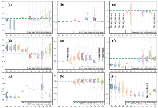
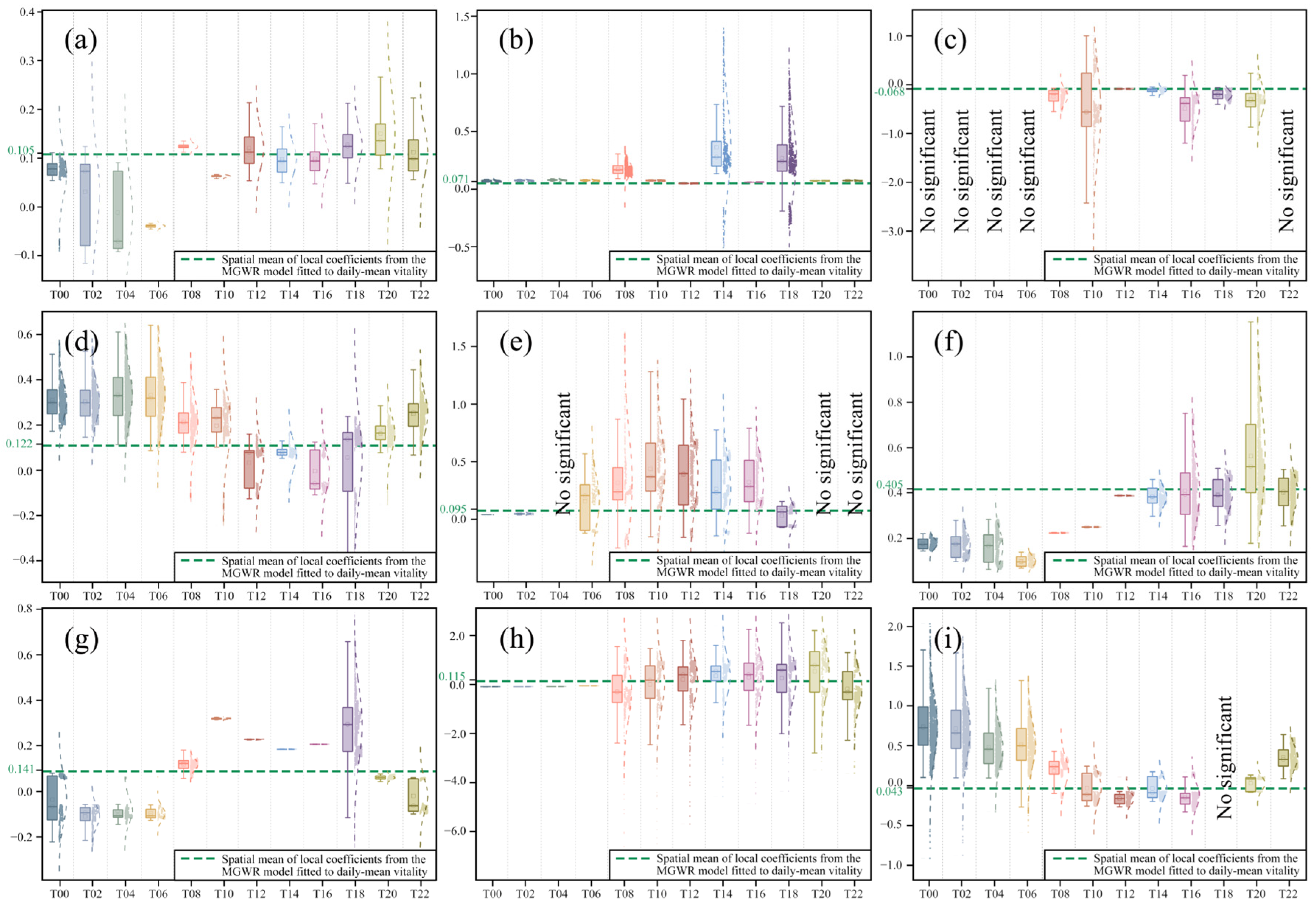
To specify the interpretive information provided by the two-hourly models, Figure 6 places each time-specific local coefficient distribution against an aggregate reference derived from the daily mean MGWR. The benchmark was constructed in two sequential steps. First, the twelve vitality values for each parcel were averaged to form a daily mean dependent variable. Second, MGWR was fitted to this daily mean outcome using the same explanatory variables, and the spatial mean of the resulting local coefficients was plotted as the green dashed line. The box–violin plots represent the local coefficient distributions from the twelve primary time-specific models. The averaging therefore occurs in the vitality outcome before regression. All temporal descriptions below refer to the coefficients associated with each built-environment variable, whose measured values remain fixed across the daily cycle.

Figure 6. Two-hourly MGWR local coefficient distributions relative to the daily mean benchmark. (a) Road betweenness; (b) road network integration; (c) distance to the nearest metro station; (d) residential land percentage; (e) commercial land percentage; (f) kernel density of catering POIs; (g) kernel density of enterprise POIs; (h) kernel density of shopping service POIs; (i) kernel density of life service facility POIs. The box–violin plots summarize the local coefficient distributions from the twelve time-specific MGWR models. The green dashed line represents the spatial mean of the local coefficients from the MGWR model fitted to daily mean vitality.

The transport-related coefficients show clear differences in temporal position, magnitude, and local spread (Figure 6a–c). The coefficient distributions associated with road betweenness (X1) were mainly below the daily mean reference from 00:00 to 06:00. They approached or exceeded the reference around 08:00, 12:00, 18:00, and 20:00, with broader local variation during selected early-morning and evening periods. Road network integration (X2) remained close to or below its benchmark during most periods but showed pronounced increases at 08:00, 14:00, and 18:00; the distributions at 14:00 and 18:00 were also more dispersed. Distance to the nearest metro station (X3) had a negative benchmark coefficient. Its clearest time-specific coefficient distributions occurred between 08:00 and 20:00 and were predominantly positioned below the benchmark, indicating stronger negative associations during these periods. Because X3 is a distance measure, the more negative coefficients correspond to a stronger association between metro-station proximity and urban vitality.

The land-use coefficients display contrasting temporal profiles for residential and commercial functions (Figure 6d,e). The coefficient distributions associated with residential land percentage (X4) were generally above the benchmark from 00:00 to 10:00, declined from 12:00 to 18:00, and rose again after 20:00. Several midday and afternoon distributions included negative values, indicating increased local differentiation. Commercial land percentage (X5) showed its most pronounced coefficient distributions from 06:00 to 18:00. Its coefficients were predominantly positive and generally above the benchmark from 08:00 to 16:00, followed by a marked decline at 18:00. The two-hourly results therefore distinguish an extended late-night and morning association for residential land from a predominantly daytime association for commercial land.

The functional-facility coefficients reveal further temporal differentiation among facility types (Figure 6f–i). Catering POI density (X6) remained below the benchmark during the early part of the day, approached it during the afternoon, and reached its strongest and most dispersed positive distribution at 20:00. Enterprise POI density (X7) changed from negative coefficient distributions during 00:00–06:00 to distributions above the benchmark during much of 10:00–18:00, followed by a decline at 20:00 and a return to negative values at 22:00. Shopping-service POI density (X8) showed relatively compact coefficients during the early periods and much wider distributions from 08:00 onward, with positive and negative values occurring within the same periods. Life-service POI density (X9) showed coefficient distributions above the benchmark from 00:00 to 08:00, shifted to negative values during 12:00–16:00, approached the benchmark around 20:00, and became strongly positive again at 22:00.

The daily mean benchmark summarizes the aggregate coefficient level, while the primary two-hourly models resolve when each association strengthens, weakens, changes direction, or becomes locally differentiated. Their added interpretive value is therefore expressed through variable-specific temporal windows and time-varying local coefficient distributions. These temporal patterns provide the basis for the subsequent spatial analysis in Section 3.5.

3.5. Spatiotemporal Patterns of Two-Hourly Local Built-Environment–Vitality Associations

Section 3.4 identifies the periods in which the time-specific coefficient distributions depart from the daily mean reference. Figure 7 further show where statistically significant local coefficients occurred and how their spatial coverage varied among the displayed periods. Because the built-environment measurements remained fixed throughout the modeled cycle, these visualizations represent coefficient surfaces estimated for successive two-hourly vitality outcomes. The following analysis is therefore limited to coefficient direction, magnitude, spatial distribution, and temporal occurrence.

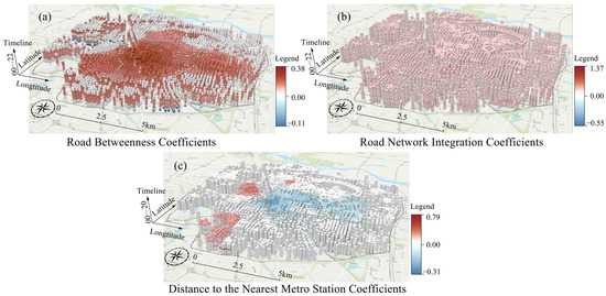
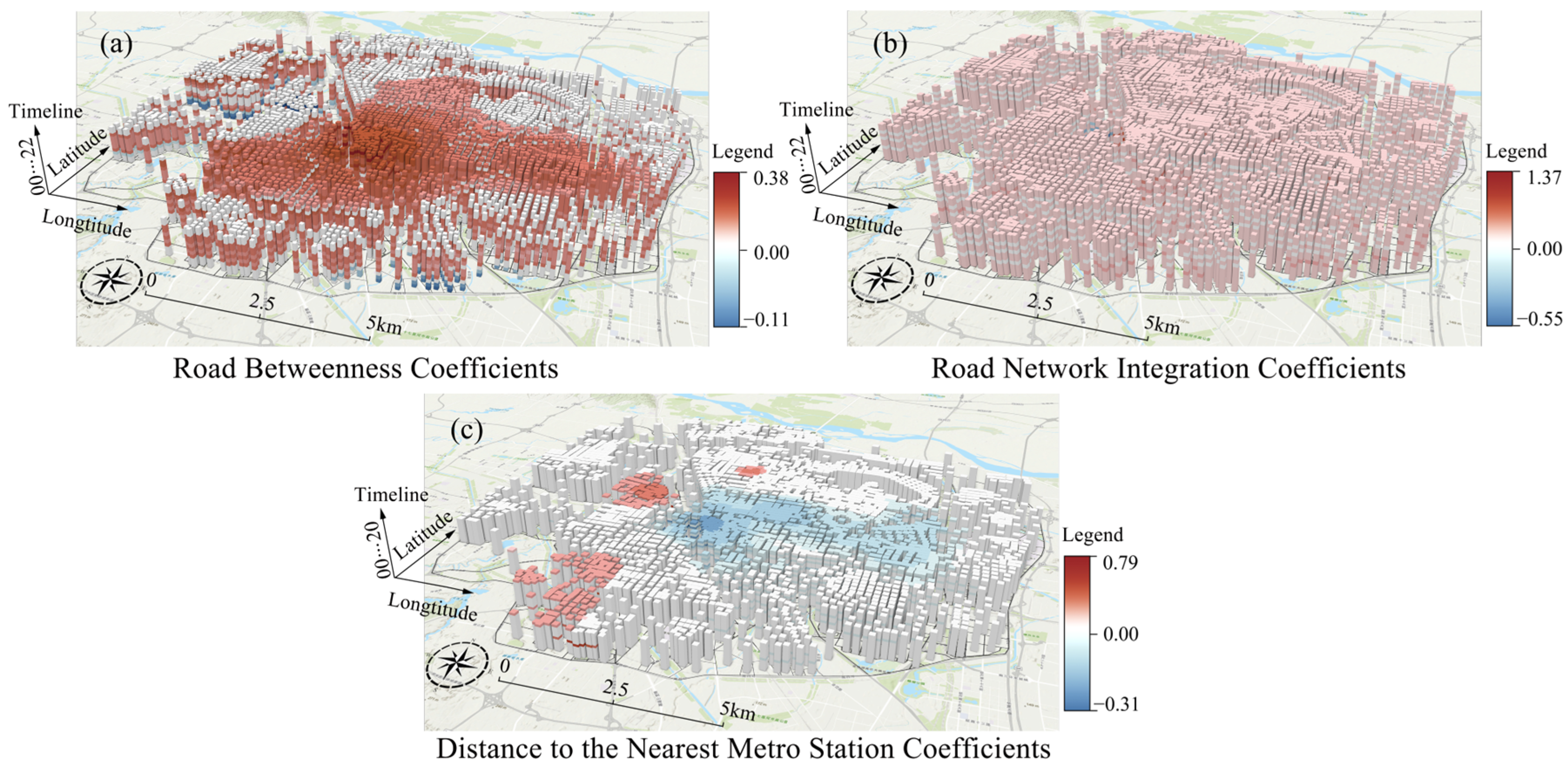
Figure 7. Space–time distribution of significant MGWR coefficients for the transport-related variables. (a) Road betweenness coefficients; (b) road network integration coefficients; and (c) distance to the nearest metro-station coefficients. Colors represent the direction and magnitude of the significant MGWR coefficients, while the vertical dimension represents time. To emphasize statistically significant spatiotemporal patterns, only time slices with significant coefficients (p < 0.05) are displayed. Consequently, the temporal extent of the cubes may differ among variables, and the uppermost layer does not necessarily correspond to the 22:00 time slice.

3.5.1. Spatiotemporal Patterns of Transport-Related Associations

The transport-related coefficient surfaces differed in their spatial extent and configuration. Significant coefficients for road betweenness (X1) and road-network integration (X2) covered relatively broad areas and corridors, whereas those for distance to the nearest metro station (X3) were concentrated along rail-transit corridors and around selected stations (Figure 7).

Significant road-betweenness coefficients occurred mainly in the central urban area and in parcels located along major road corridors. Positive coefficients were concentrated in the central and eastern parts of the study area, while significant coefficients in peripheral areas were more scattered. Their occurrence across multiple time slices indicates that the spatial correspondence between road betweenness and vitality was present during several periods of the sampled daily cycle.

Road-network integration produced a broader and more spatially continuous coefficient pattern. Significant coefficients were predominantly positive, and their local magnitudes increased during several daytime periods. The extent and magnitude of these coefficients show that the statistical association between network integration and vitality varied both temporally and spatially, although the underlying road-network indicator remained unchanged.

Coefficients for distance to the nearest metro station were more spatially selective. Significant values were concentrated in the central urban area, along rail-transit corridors, and around selected stations. Their predominantly negative direction indicates that parcels closer to metro stations tended to have higher vitality after accounting for the other explanatory variables. These coefficients describe a localized association with station proximity; interpretations involving actual station use, route choice, or trip purpose require transport-behavior data.

3.5.2. Spatiotemporal Patterns of Land-Use Associations

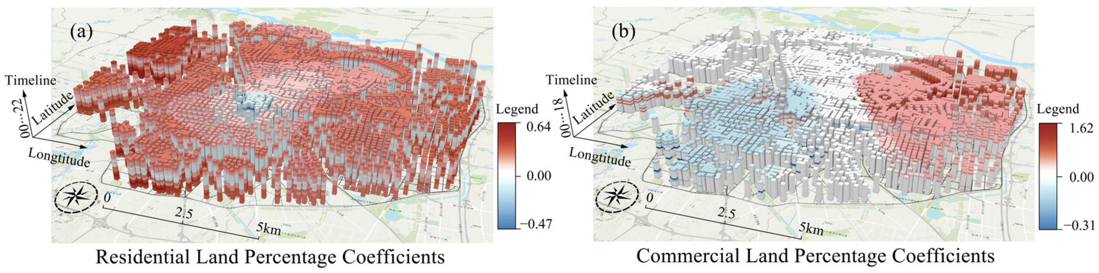
The land-use coefficient surfaces showed a contrast between the extensive distribution associated with residential land and the more spatially concentrated distribution associated with commercial land (Figure 8). This contrast concerns the estimated associations of the two land-use variables with vitality across the study area.

Figure 8. Space–time distribution of significant MGWR coefficients for the land-use variables. (a) Residential land percentage coefficients and (b) commercial land percentage coefficients. Colors represent the direction and magnitude of the significant MGWR coefficients, while the vertical dimension represents time. Only statistically significant time slices (p < 0.05) are shown; therefore, the temporal extent of the cubes varies among variables, and the uppermost layer does not necessarily represent the 22:00 time slice.

Significant coefficients for residential land percentage (X4) covered a large proportion of the study area and were spatially continuous during multiple time slices. Their general spatial distribution remained comparatively stable, with localized changes around the central urban area. The temporal differences were expressed primarily through changes in coefficient magnitude and direction rather than through changes in the residential-land surface itself.

Commercial land percentage (X5) showed greater spatial selectivity. Positive coefficients were concentrated mainly in the eastern and northeastern parts of the study area and around several commercial agglomeration areas, whereas negative coefficients occurred in parts of the central and western areas. These contrasting coefficient directions indicate that the local association between commercial land percentage and vitality varied across surrounding spatial contexts.

3.5.3. Spatiotemporal Patterns of Facility-Related Associations

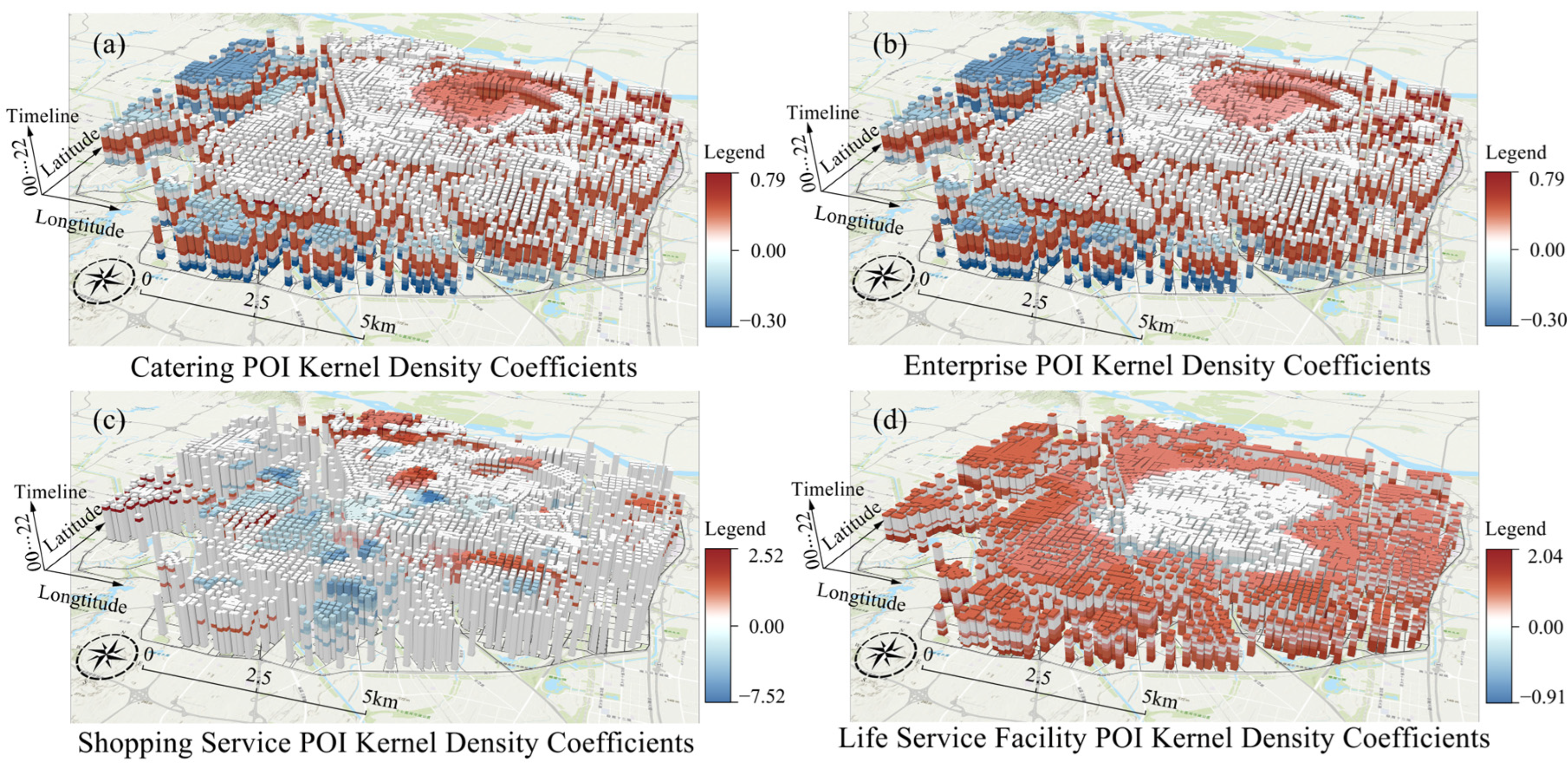
The four facility variables exhibited distinct coefficient distributions in spatial extent, direction, magnitude, and temporal occurrence (Figure 9). These differences show that the statistical relationships between vitality and the measured facility categories were locally and temporally differentiated.

Figure 9. Space–time distribution of significant MGWR coefficients for the facility-related variables. (a) Catering POIs kernel density coefficients; (b) enterprise POIs kernel density coefficients; (c) shopping service POIs kernel density coefficients; and (d) life service facility POIs kernel density coefficients. Colors represent the direction and magnitude of the significant MGWR coefficients, while the vertical dimension represents time. Only statistically significant time slices (p < 0.05) are retained for visualization. As a result, the temporal extent of the cubes may vary among POI categories, and the uppermost layer does not necessarily correspond to the 22:00 time slice.

Significant coefficients for catering POI density (X6) were concentrated in central and eastern districts and around several peripheral nodes. Enterprise POI density (X7) showed a broadly similar spatial extent across the central urban area, eastern districts, and several areas with concentrated enterprise POIs. Their temporal coefficient sequences nevertheless differed, indicating that similar spatial coverage can coexist with different time-specific association patterns.

Shopping-service POI density (X8) produced relatively localized but widely dispersed coefficient values. Positive coefficients occurred mainly in northern and eastern districts and around several commercial nodes, while negative coefficients appeared in parts of the central and peripheral areas. The coexistence of positive and negative values indicates substantial local differentiation in the association between shopping-service POI density and vitality.

Life-service POI density (X9) produced the broadest spatial coverage among the four facility variables. Significant coefficients occurred across a large proportion of parcels and were predominantly positive during multiple periods. Taken together, the facility-related results distinguish the comparatively extensive associations of life-service POIs from the more spatially selective coefficient patterns of catering, enterprise, and shopping-service POIs.

4. Discussion

4.1. Comparison with Previous Studies and Study Contributions

The broad directions of the associations identified in Zhengzhou are consistent with previous urban-vitality studies. Road betweenness and road-network integration were predominantly positively associated with vitality [34], while shorter distance to metro stations corresponded to higher vitality in several periods [25]. Residential land, commercial land, and the four facility categories also showed significant local associations [2,26], broadly consistent with evidence that transport conditions, land-use composition, and facility concentration are important spatial correlates of urban activity. This agreement establishes the empirical context for interpreting the finer temporal differences identified in Zhengzhou.

The twelve two-hourly models provide the study’s added analytical information by resolving the aggregate daily relationship into successive local coefficient distributions. The daily mean MGWR achieved an R² of 0.791 and provides an internally consistent aggregate reference. Because the parcels, explanatory variables, and modeling framework are identical, comparison with this reference isolates the information associated with temporal disaggregation of the vitality outcome. The two-hourly results identify when coefficients strengthen or weaken, change direction, and become more or less locally dispersed.

This evidence extends previous studies that examined spatial non-stationarity [4,18] or differences between broad day and night categories [2,25,26]. Combining twelve observation times with parcel-scale MGWR shows that intra-day variation is expressed through changes in coefficient magnitude, direction, spatial extent, and local dispersion. The contribution therefore lies in characterizing the temporal expression of local spatial heterogeneity at a resolution summarized into a single representation by the daily mean model.

4.2. Interpretation of Time-Conditioned Local Associations

The temporal coefficient patterns describe how successive vitality distributions are statistically related to the same built-environment configuration. Road betweenness, road-network integration, metro-station distance, land-use percentages, and POI densities retain identical measured values across the twelve models. The changing quantities are the two-hourly vitality outcome and the local coefficients estimated between that outcome and each fixed explanatory-variable surface.

The transport-related results illustrate this distinction. More positive coefficients for road-network integration during selected daytime periods indicate a closer statistical correspondence between network integration and daytime vitality distributions. More negative coefficients for metro-station distance from 08:00 to 20:00 indicate a stronger association between station proximity and vitality during these periods. These temporal differences concern the estimated relevance of fixed network and station-proximity conditions. Explanations involving route choice, actual station use, or trip purpose require passenger-flow, trajectory, or travel-survey data.

The land-use results show corresponding time-conditioned associations. Residential-land coefficients were generally more positive during late-night, early-morning, and later-evening periods, whereas commercial-land coefficients were more pronounced during the daytime. The residential and commercial land surfaces remained unchanged, and their contrasting profiles were produced by relating those fixed surfaces to successive vitality distributions.

The facility-related coefficients also followed distinct temporal profiles. Catering, enterprise, shopping-service, and life-service POI densities retained the same spatial values throughout the daily cycle, while their estimated associations with vitality varied among periods and locations. These results establish temporal and local statistical differentiation among the measured facility categories. Direct interpretation of facility use or individual activity purpose requires behavior-specific observations.

4.3. Implications for Time-Sensitive Urban Management and Relevance to Long-Term Planning

The most direct practical implication of the two-hourly analysis concerns time-sensitive urban management. The time-specific MGWR coefficient distributions identify when and where associations with transport-related spatial conditions, land-use composition, and facility configuration become stronger or weaker, change direction, or exhibit greater spatial differentiation. The corresponding vitality surfaces describe the observed intensity and spatial concentration of population activity. Reading these two outputs together distinguishes areas with persistent activity concentration from those whose activity patterns and associated spatial conditions become pronounced during particular periods. This evidence provides a period- and area-specific basis for prioritizing monitoring and contextual diagnosis.

The relevance to spatial planning lies in adding a temporal dimension to the evaluation of existing urban configurations. The daily mean model summarizes the aggregate relationships of vitality with transport, land-use, and facility conditions, while the two-hourly models distinguish associations that remain broadly sustained across the daily cycle from those concentrated in particular periods or characterized by directional and local changes. Reading these results together supports a more differentiated assessment of how existing spatial arrangements correspond to both overall and time-specific activity patterns. Within this framework, the daily mean model provides the aggregate reference, and the two-hourly models provide the additional planning-relevant information.

4.4. Limitations and Future Research

Despite revealing the spatiotemporal variation in urban vitality and its built-environment associations at two-hour intervals, this study has several limitations. First, the temporal representativeness of the data can be further improved. Urban vitality was derived primarily from Baidu Heatmap data collected on ten sampling dates. Although multi-day averaging helps reduce random daily fluctuations, differences between weekdays and weekends, periods surrounding the Spring Festival, and weather conditions may still affect population activity. The results should therefore be interpreted primarily as average intra-day patterns within the selected winter observation window. Future studies could extend the observation period and compare different seasons and day types using multiple sources of population-activity data. Related research has similarly noted that short observation periods may limit the identification of longer-term variation in built-environment–vitality relationships and has recommended validation using longer-term datasets.

Second, the modal coverage of the transport-related variables and the behavioral interpretation of the vitality data remain limited. Road betweenness and road-network integration characterize the topology of the fixed road network, while distance to the nearest metro station characterizes station proximity. These indicators do not represent observed motor-vehicle flows, actual metro use, or accessibility through all travel modes. Temporally consistent information on bus-stop locations and service frequencies, pedestrian-network accessibility, and cycling conditions was unavailable for the observation period. Future studies could integrate these dimensions with traffic-flow data, mobile-phone signaling, trajectory data, and travel surveys to provide a more comprehensive representation of multimodal accessibility. Baidu Heatmap data record population-activity intensity but do not identify individual activity purposes; behavior-specific interpretations therefore require complementary mobility or survey data.

Third, the generalizability of the identified relationships requires further validation. The analysis focuses on the central urban area of Zhengzhou, and the observed coefficient patterns may reflect the city’s particular spatial structure, transport system, and functional configuration. Previous cross-city research has shown that the same built-environment indicators can exhibit different associations with vitality across urban contexts. MGWR also identifies local statistical associations rather than causal effects. Future multi-city and multi-scale comparisons, longer observation periods, and complementary behavioral datasets could further test the robustness and transferability of the relationships identified in this study.

5. Conclusions

Using Baidu Heatmap-derived activity intensity and multi-source built-environment data, this study examined two-hourly urban vitality dynamics and the spatiotemporal heterogeneity of local built-environment–vitality associations in central Zhengzhou. Twelve time-specific MGWR models formed the primary analysis, while a daily mean MGWR provided an aggregate benchmark for identifying the interpretive information added by the two-hourly results. The main conclusions are as follows:

(1)

Urban vitality followed a clear intra-day rhythm while remaining anchored in a persistent center–corridor–node spatial structure. The two-hourly Global Moran’s I values ranged from 0.508 to 0.562 and identified stage-specific changes in spatial clustering, including a morning minimum and an evening local trough. The daily mean Moran’s I of 0.559 provided an aggregate reference for this persistent clustering pattern.

(2)

The two-hourly MGWR models explained 69.1–81.8% of the spatial variation in vitality and generally outperformed the corresponding OLS models. The daily mean MGWR achieved an R² of 0.791 and captured the aggregate spatial relationship effectively. Relative to this benchmark, the two-hourly models identified variable-specific association windows, changes in coefficient direction, and time-varying local dispersion. Metro-proximity associations were strongest from 08:00 to 20:00; residential and commercial land followed contrasting temporal profiles; and catering, enterprise, shopping, and life-service facilities exhibited distinct periods of local differentiation.

(3)

The local associations also differed in spatial extent and temporal persistence. Road-network variables generally showed broad corridor- and area-based patterns, while metro-related coefficients were concentrated along rail-transit corridors and around selected stations. Residential land and life-service facilities showed relatively extensive associations, whereas commercial land and specialized facility categories were more concentrated around functional nodes. Together, these results show that the spatial extent and temporal occurrence of local built-environment–vitality associations varied across the successive two-hourly vitality distributions.

Using the daily mean MGWR as an aggregate reference, the twelve two-hourly models reveal additional information about when, where, and in what direction local built-environment–vitality associations vary. This evidence supports period- and area-specific urban monitoring and adds a temporal dimension to the evaluation of existing transport, land-use, and facility configurations. The study’s analytical contribution therefore lies in distinguishing aggregate spatial relationships from their intra-day expression at the parcel scale.

References

- Wang, M.; Zhao, J.; Zhang, D.; Xiong, Z.; Sun, C.; Zhang, M.; Fan, C. Assessing urban vitality in high-density cities: A spatial accessibility approach using POI reviews and residential data. Humanit. Soc. Sci. Commun. 2025, 12, 1119. [Google Scholar] [CrossRef] [Scilit]
- Zhang, Y.; Wang, X.; Wang, L.; Zhang, Y.; Ye, Y.; Jiang, H.; Chi, Y.; Liu, G.; Yao, S. Measurement of urban vitality and the influence mechanism of the built environment on it based on multi-source data: A case study of Yantai City. PLoS ONE 2026, 21, e0343003. [Google Scholar] [CrossRef] [Scilit] [PubMed]
- Tang, S.; Ta, N. How the built environment affects the spatiotemporal pattern of urban vitality: A comparison among different urban functional areas. Comput. Urban Sci. 2022, 2, 39. [Google Scholar] [CrossRef] [Scilit] [PubMed]
- Lyu, G.; Angkawisittpan, N.; Fu, X.; Sonasang, S. Investigating the relationship between built environment and urban vitality using big data. Sci. Rep. 2025, 15, 579. [Google Scholar] [CrossRef] [Scilit] [PubMed]
- Jin, A.; Ge, Y.; Zhang, S. Spatial Characteristics of Multidimensional Urban Vitality and Its Impact Mechanisms by the Built Environment. Land 2024, 13, 991. [Google Scholar] [CrossRef] [Scilit]
- Xia, X.; Zhang, Y.; Zhang, Y.; Rao, T. The Spatial Pattern and Influence Mechanism of Urban Vitality: A Case Study of Changsha, China. Front. Environ. Sci. 2022, 10, 942577. [Google Scholar] [CrossRef] [Scilit]
- Kim, Y.-L. Urban Vitality Measurement Through Big Data and Internet of Things Technologies. ISPRS Int. J. Geo-Inf. 2025, 14, 14. [Google Scholar] [CrossRef] [Scilit]
- Pan, J.; Zhu, X.; Zhang, X. Urban Vitality Measurement and Influence Mechanism Detection in China. Int. J. Environ. Res. Public Health 2023, 20, 46. [Google Scholar] [CrossRef] [Scilit] [PubMed]
- Liu, S.; Ge, J.; Ye, X.; Wu, C.; Bai, M. Urban Vitality Assessment at the Neighborhood Scale with Geo-Data: A Review toward Implementation. J. Geogr. Sci. 2023, 33, 1482–1504. [Google Scholar] [CrossRef] [Scilit]
- Collins, T.; Di Clemente, R.; Gutiérrez-Roig, M.; Botta, F. Spatiotemporal Gender Differences in Urban Vibrancy. Environ. Plan. B Urban Anal. City Sci. 2024, 51, 1430–1446. [Google Scholar] [CrossRef] [Scilit]
- Liu, M.; Li, R.; Zhang, B.; Li, Y. Supply–Demand Relationship between Nighttime Lighting and Urban Vitality Based on Multi-Source Data. Indoor Built Environ. 2026, 35, 101–121. [Google Scholar] [CrossRef] [Scilit]
- Chen, H.; Ge, J.; He, W. Quantifying Urban Vitality in Guangzhou through Multi-Source Data: A Comprehensive Analysis of Land Use Change, Streetscape Elements, POI Distribution, and Smartphone-GPS Data. Land 2025, 14, 1309. [Google Scholar] [CrossRef] [Scilit]
- Wu, W.; Xu, L.; Zhao, K. Urban Vitality and Built Environment from the Perspective of Spatiotemporal Heterogeneity. Spat. Econ. Anal. 2025, 20, 218–241. [Google Scholar] [CrossRef] [Scilit]
- Kang, C.; Fan, D.; Jiao, H. Validating Activity, Time, and Space Diversity as Essential Components of Urban Vitality. Environ. Plan. B Urban Anal. City Sci. 2021, 48, 1180–1197. [Google Scholar] [CrossRef] [Scilit]
- Sheng, J.; He, Y.; Lu, T.; Wang, F.; Huang, Y.; Leng, B.; Zhang, X.; Chen, Y. Exploring Urban Vitality Characteristics and Interactive Mechanisms at the Community Scale through the Lens of Human Behaviour: A Case Study of Chongqing, China. ISPRS Ann. Photogramm. Remote Sens. Spat. Inf. Sci. 2024, 10, 303–310. [Google Scholar] [CrossRef] [Scilit]
- Mouratidis, K.; Poortinga, W. Built Environment, Urban Vitality and Social Cohesion: Do Vibrant Neighborhoods Foster Strong Communities? Landsc. Urban Plan. 2020, 204, 103951. [Google Scholar] [CrossRef] [Scilit]
- Zhang, C.; Li, W.; Zhang, S.; Wang, X.; Hu, J.; Fan, Q.; Wang, Q. Multifractal analysis of heritage architecture: Quantifying complexity in 30 iconic historic buildings. npj Herit. Sci. 2026, 14, 497. [Google Scholar] [CrossRef] [Scilit]
- Lu, X.; Huang, S.; Xie, W.; Sun, Y. The Impact of Built Environment on Urban Vitality—A Multi-Scale Geographically Weighted Regression Analysis in the Case of Shenyang, China. Buildings 2025, 15, 2989. [Google Scholar] [CrossRef] [Scilit]
- Wu, Y.; Xie, C.; Zhang, A.; Zhao, T.; Cao, J. Spatiotemporal Analysis of Urban Vitality and Its Drivers from a Human Mobility Perspective. ISPRS Int. J. Geo-Inf. 2025, 14, 167. [Google Scholar] [CrossRef] [Scilit]
- Xia, C.; Yeh, A.G.O.; Zhang, A. Analyzing Spatial Relationships between Urban Land Use Intensity and Urban Vitality at Street Block Level: A Case Study of Five Chinese Megacities. Landsc. Urban Plan. 2020, 193, 103669. [Google Scholar] [CrossRef] [Scilit]
- He, J.; Liu, P.; Li, X. Modeling Multi-Type Urban Landscape Dynamics along the Horizontal and Vertical Dimensions. Landsc. Urban Plan. 2023, 233, 104683. [Google Scholar] [CrossRef] [Scilit]
- McMillen, D.P. Geographically Weighted Regression: The Analysis of Spatially Varying Relationships. Am. J. Agric. Econ. 2004, 86, 554–556. [Google Scholar] [CrossRef] [Scilit]
- Fotheringham, A.S.; Yang, W.; Kang, W. Multiscale Geographically Weighted Regression (MGWR). Ann. Am. Assoc. Geogr. 2017, 107, 1247–1265. [Google Scholar] [CrossRef] [Scilit]
- Oshan, T.M.; Li, Z.; Kang, W.; Wolf, L.J.; Fotheringham, A.S. mgwr: A Python Implementation of Multiscale Geographically Weighted Regression for Investigating Process Spatial Heterogeneity and Scale. ISPRS Int. J. Geo-Inf. 2019, 8, 269. [Google Scholar] [CrossRef] [Scilit]
- Li, Z.; Zhao, G. Revealing the spatio-temporal heterogeneity of the association between the built environment and urban vitality in Shenzhen. ISPRS Int. J. Geo-Inf. 2023, 12, 433. [Google Scholar] [CrossRef] [Scilit]
- Liu, J.; Li, Y.; Xu, Y.; Zhuang, C.C.; Hu, Y.; Yu, Y. Impacts of built environment on urban vitality in cultural districts: A case study of Haikou and Suzhou. Land 2024, 13, 840. [Google Scholar] [CrossRef] [Scilit]
- Wu, Y.; Yuan, J. Is There a Regulation in the Expansion of Urban Spatial Structure? Empirical Study from the Main Urban Area in Zhengzhou, China. Sustainability 2022, 14, 2883. [Google Scholar] [CrossRef] [Scilit]
- Shen, W.; Li, P.; Yao, W.; Zhao, X.; Ren, Y.; Zheng, Y.; Jiang, Y. The Structural Characteristics and Spatial Organization Pattern of China’s Urban Network Based on the Multiple Flow. Geogr. Res. 2023, 42, 514–533. [Google Scholar]
- Moran, P.A.P. Notes on Continuous Stochastic Phenomena. Biometrika 1950, 37, 17–23. [Google Scholar] [CrossRef] [Scilit]
- Anselin, L. Local Indicators of Spatial Association—LISA. Geogr. Anal. 1995, 27, 93–115. [Google Scholar] [CrossRef] [Scilit]
- Kang, W.; Oshan, T.M. Scale and Correlation in Multiscale Geographically Weighted Regression (MGWR). J. Geogr. Syst. 2025, 27, 399–424. [Google Scholar] [CrossRef] [Scilit]
- Anselin, L.; Rey, S. Properties of Tests for Spatial Dependence in Linear Regression Models. Geogr. Anal. 1991, 23, 112–131. [Google Scholar] [CrossRef] [Scilit]
- Wu, J.; Tu, Y.; Chen, Z.; Yu, B. Analyzing the Spatially Heterogeneous Relationships between Nighttime Light Intensity and Human Activities across Chongqing, China. Remote Sens. 2022, 14, 5695. [Google Scholar] [CrossRef] [Scilit]
- Lu, S.; Shi, C.; Yang, X. Impacts of built environment on urban vitality: Regression analyses of Beijing and Chengdu, China. Int. J. Environ. Res. Public Health 2019, 16, 4592. [Google Scholar] [CrossRef] [Scilit] [PubMed]
Disclaimer/Publisher’s Note: The statements, opinions and data contained in all publications are solely those of the individual author(s) and contributor(s) and not of MDPI and/or the editor(s). MDPI and/or the editor(s) disclaim responsibility for any injury to people or property resulting from any ideas, methods, instructions or products referred to in the content. |
© 2026 by the authors. Published by MDPI on behalf of the International Society for Photogrammetry and Remote Sensing. Licensee MDPI, Basel, Switzerland. This article is an open access article distributed under the terms and conditions of the Creative Commons Attribution (CC BY) license.