A Multi-Task Framework for Vehicle Trajectory and Disturbance Classification in Autonomous Driving Scenarios

Abstract

Systematic scenario classification supports the characterization of test conditions in simulation-based autonomous driving validation. This paper proposes a multi-task framework that combines OpenSCENARIO text embeddings with Ego-vehicle motion representations learned by Autoencoders trained on the SinD real-world dataset. The framework jointly predicts trajectory type and binary perception and decision disturbances, defined using environmental conditions and collision occurrence, respectively. We evaluate 24 combinations of four text encoders and six trajectory Autoencoders under fixed and uncertainty-based task weighting. On generated test scenarios with modified temporal and environmental parameters, Qwen3-Embedding-0.6B combined with Mamba-AE achieves the highest Full Match Accuracy of 91.61%, requiring all three labels to be predicted correctly, and trajectory accuracy of 99.97% under fixed weighting. Perception classification limits joint performance, and high validation accuracy does not consistently extend to the modified test conditions. Uncertainty-based weighting provides no consistent improvement, while latent-vector ablations show task-dependent contributions from text and motion representations. These findings support offline classification within the evaluated scenario configurations while identifying limitations in robustness to parameter changes.

1. Introduction

With the rapid advancement of autonomous driving technology, the importance of validating vehicle safety and reliability has grown significantly [1,2,3]. In particular, testing autonomous vehicles in real-world environments requires ensuring safety in hazardous situations, a requirement that is also emphasized in functional safety standards such as ISO 26262 [4]. However, real-world validation entails substantial time and economic costs, and repeated experimentation is inherently difficult. To address these challenges, simulation-based validation methods that replicate real-world environments have been actively studied. Simulators such as CARLA (https://carla.org/ (accessed on 11 August 2026)), esmini (https://github.com/esmini (accessed on 11 August 2026)), and MORAI (https://www.morai.ai/ (accessed on 11 August 2026)) enable repeated reproduction of diverse driving situations with user-defined environment configurations, facilitating efficient generation of driving and accident scenarios across a wide range of spatiotemporal conditions [1,5,6].

However, when simulation-based scenarios are generated without a systematic classification framework, characterizing individual scenarios and analyzing validation results becomes difficult. In particular, identifying vulnerabilities in autonomous driving systems requires structural comparison and systematic categorization of scenarios. Accordingly, there is a clear need for a method that can define and classify scenarios according to consistent criteria. Existing approaches include the layer-based classification framework proposed by the Pegasus project and ontology-based methods. However, since these approaches primarily define scenarios around environmental conditions and objects, they suffer from increasing complexity and limited scalability when new elements are introduced.

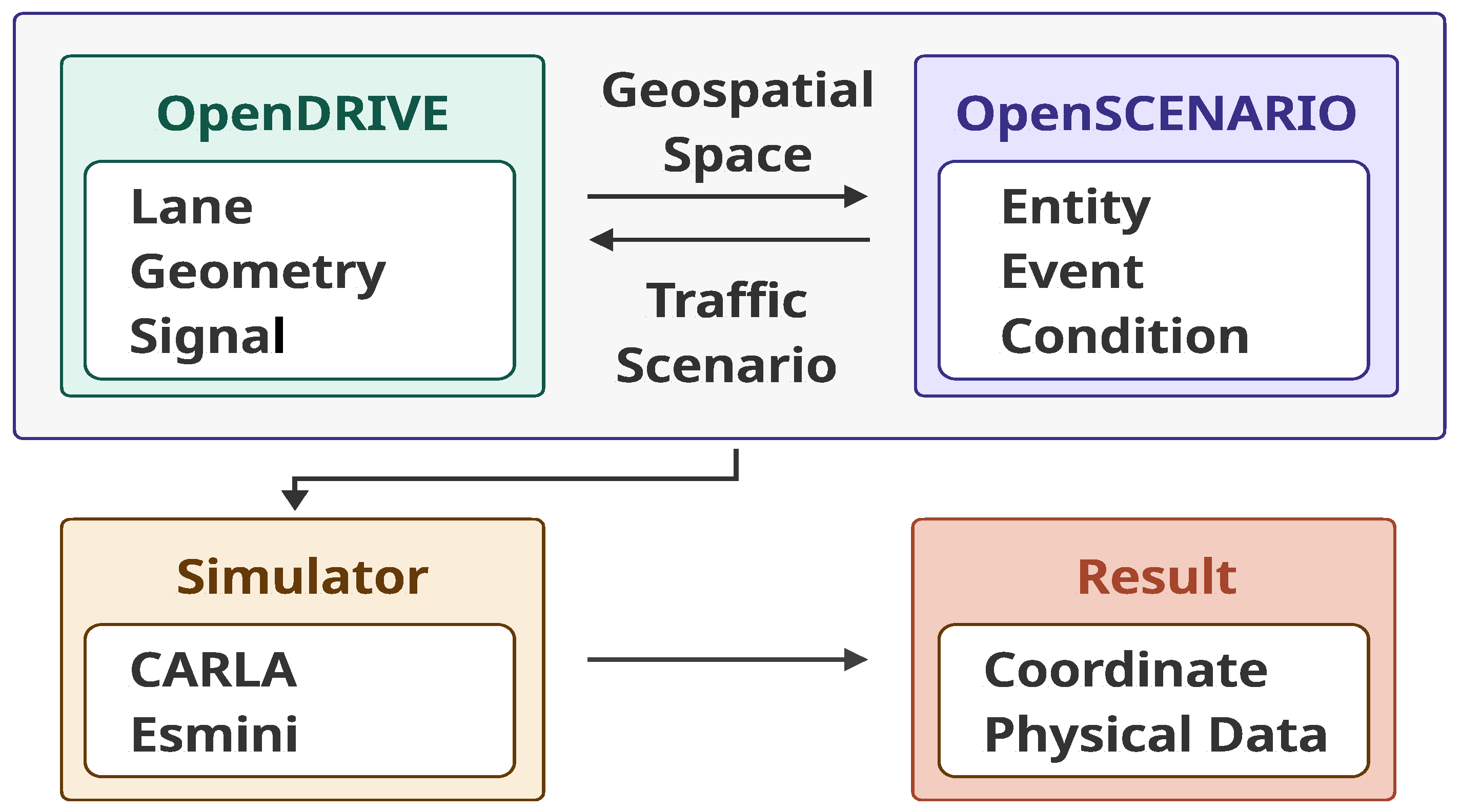
Widely used standards in autonomous driving simulation include OpenSCENARIO (https://www.asam.net/standards/detail/openscenario-xml/ (accessed on 11 August 2026)) and OpenDRIVE (https://www.asam.net/standards/detail/opendrive/ (accessed on 11 August 2026)), both proposed by the Pegasus project (https://www.pegasusprojekt.de/en/home (accessed on 11 August 2026)). OpenSCENARIO employs an XML-based structure to define environmental settings, object creation and control, and success/failure conditions within a scenario, and is used to represent dynamic elements in simulation. OpenDRIVE, on the other hand, defines the static environment including road networks, lane structures, and intersection information. The overall structure of these standards is illustrated in Figure 1. Various simulators adopt different map representations based on these standards; for example, CARLA and esmini use OpenDRIVE, while Autoware Foundation (https://github.com/autowarefoundation (accessed on 11 August 2026)) utilizes Lanelet2-based maps [7]. These systems commonly define the space in which vehicles and pedestrians can move, and construct driving routes based on road connectivity.

Previous studies have investigated the use of real-world driving data for scenario extraction, simulation scenario construction, and comparison of simulated and observed vehicle behavior [1,5,8,9,10]. Recent work has also explored the generation of safety-critical scenarios from real-world pre-crash trajectories [11]. These efforts provide foundations for constructing test cases and motivate complementary classification methods for organizing the resulting scenarios. Our prior work classified scenarios using vehicle trajectories [12]. However, trajectory types alone do not describe the environmental conditions or collision-related outcomes associated with a maneuver. This study proposes an integrated framework for classifying intersection scenarios by combining structured OpenSCENARIO information with Ego-vehicle motion representations learned from the SinD dataset. The framework jointly predicts trajectory type, perception-related environmental conditions, and collision-related outcomes used as decision-disturbance labels. These outputs characterize scenario conditions and observed outcomes rather than directly diagnosing failures in individual autonomous driving components.

The contributions of this study are threefold. First, a multi-task classification framework combines trajectory and disturbance labels within a shared representation and prediction pipeline. Second, the framework is evaluated across 24 text–trajectory encoder combinations and two task-weighting strategies to examine their effects on individual-task and joint classification performance. Third, separately generated test scenarios with modified parameters and latent-vector ablations are used to evaluate performance under changed parameter configurations and assess input dependence within the trained classifier. The remainder of the paper is organized as follows. Section 2 introduces related work. Section 3 describes the dataset and proposed method. Section 4 presents experimental results. Section 5 concludes the paper and discusses future research directions.

2. Related Work

This section reviews prior studies related to scenario classification, disturbance characterization, and standardized safety testing for autonomous driving. Text encoding and variable-length time-series modeling are then reviewed as approaches for representing scenario context and vehicle motion.

2.1. Scenario Classification for Autonomous Driving

Various studies have been conducted to systematically define and classify autonomous driving scenarios. Layer-based approaches organize scenario components into categories describing road infrastructure, environmental conditions, and dynamic objects [13,14]. Such structures provide a systematic description of scenario composition, while further characterization is needed to distinguish the behaviors and interactions occurring within these components. Ontology-based approaches have also been proposed to represent relationships between surrounding objects and describe scenario interactions in a structured manner [15]. Naturalistic driving studies have also examined vehicle behavior in relation to its spatial context. Geographic Information Systems have been used to extract driving patterns from kinematic measurements across different spatial scales, relating vehicle behavior to the road context in which it occurs [16].

Our prior work proposed a scenario classification method based on vehicle driving trajectories and behavioral patterns, demonstrating that trajectory-centric features can serve as a practical basis for scenario classification [12]. However, its reliance on rule-based criteria required additional rules when new scenario types or conditions were introduced, and environmental disturbance factors were not incorporated into the classification. Trajectory types describe the vehicle maneuver, but do not fully characterize the conditions under which it is performed. Scenarios involving the same maneuver may differ in visibility, road conditions, and surrounding-vehicle interactions, placing different demands on autonomous driving functions. Joint characterization of vehicle behavior and disturbance factors therefore allows test scenarios to be organized according to both the maneuver and its associated conditions. The present study extends trajectory-based classification by jointly considering vehicle maneuvers, perception-related environmental conditions, and collision-related outcomes used as decision-disturbance labels.

2.2. Disturbance Factors in Autonomous Driving

Autonomous driving systems rely on sensing, decision-making, and control processes, each of which can be affected by different disturbance factors. Commonly used sensors include cameras, LiDAR, Radar, GNSS, and IMU, and their performance can vary with environmental conditions [17]. Camera-based perception is sensitive to illumination and adverse weather [18], while LiDAR and Radar can also exhibit degraded performance under unfavorable environmental conditions [19,20,21]. Previous studies have therefore investigated low illumination, adverse weather, and sensor contamination as sources of perception uncertainty [22,23,24]. These factors motivate identifying scenario conditions that may affect the reliability of perception inputs.

At the decision-making stage, surrounding-vehicle interactions can create situations requiring appropriate maneuver selection or collision avoidance. Such interactions are commonly characterized using surrogate safety measures, including Time-To-Collision (TTC), headway, and collision-related indicators [25,26,27]. These measures describe aspects of interaction risk and provide a basis for distinguishing potentially hazardous scenarios. They characterize the traffic situation, however, rather than directly establishing that an error occurred within a vehicle’s decision-making module.

In the vehicle control stage, discrepancies may arise between intended commands and actual vehicle behavior because of vehicle dynamics and road surface conditions [28]. Low-friction surfaces, for example, can affect the motion produced by a given command. Characterizing control disturbances therefore requires consideration of vehicle response and operating conditions. The same environmental factor may also affect multiple functions: adverse weather can influence both sensor observations and road friction. Consequently, functional categories describe potentially affected processes and need not be mutually exclusive.

These studies motivate organizing disturbance factors according to the autonomous driving functions they may affect. This categorization characterizes scenario conditions rather than directly diagnosing failures in individual system components. In the present study, perception and decision-related conditions are included in the classification tasks because they can be labeled using the available scenario and simulation data. Control disturbances are reviewed as part of the conceptual categorization but are excluded from classifier training and quantitative evaluation, as a validated control-disturbance labeling criterion has not been established for the present dataset. Additional continuous risk indicators for characterizing pre-collision interactions are summarized in Appendix A.

2.3. Standardized Testing and Digital Twin-Based Validation for Autonomous Vehicles

In addition to identifying disturbance factors, autonomous driving evaluation requires systematic and reproducible testing conditions. Standardized testing frameworks specify road configurations, operating conditions, and safety-critical interactions to support consistent assessment. Programs such as Euro NCAP provide defined test conditions for vehicle safety evaluation [29]. Intersection test procedures and accident-based scenario definitions provide further foundations for evaluating interactions involving crossing and turning vehicles [30,31]. These frameworks provide a basis for constructing reproducible test scenarios, while scenario classification supports organizing the resulting cases according to vehicle behavior and disturbance conditions. The two functions are complementary: standardized conditions define how scenarios are instantiated, and classification describes which maneuvers and functional challenges are represented in a test collection.

Digital twin frameworks have also been developed to support autonomous vehicle validation across different vehicle scales and operational design domains [32]. Their integration with systematic test definition, automated simulation, and performance analysis connects digital representations to validation workflows [33]. These applications highlight the potential of digital twins to serve as infrastructure for validation decisions, extending their role beyond digital replication. Scenario classification could contribute to this role by organizing simulated cases according to vehicle maneuvers, environmental conditions, and interaction outcomes. Such descriptions could support the retrieval of comparable cases, examination of scenario-category coverage, and selection of cases for further testing.

2.4. Text Encoding for Scenario Representation

Beyond defining physical and behavioral conditions, data-driven scenario classification requires contextual information to be represented in a machine-processable form. OpenSCENARIO descriptions encode scenario entities, actions, and environmental settings in structured XML, providing contextual information that complements observed vehicle motion. Transformer-based models capture contextual relationships within sequential text [34]. Pre-trained language models, including BERT, RoBERTa, and the GPT family, have demonstrated their applicability to text representation and language understanding [35,36,37]. Dedicated text embedding models have also been developed to produce vector representations for downstream tasks, offering different model sizes, embedding dimensions, and computational requirements [38,39,40,41]. These approaches provide a basis for representing textual scenario descriptions as feature vectors. For structured scenario files, the relevance of an embedding depends on its ability to retain information about scenario entities, parameters, and relationships. Text encoding can therefore provide contextual features to complement temporal representations of vehicle behavior, while input structure and sequence length remain relevant considerations.

2.5. Preprocessing for Variable-Length Time Series Data

Vehicle trajectories vary in duration across scenarios, requiring appropriate handling of variable-length time-series data. Previous studies have investigated padding, interpolation, and frequency-based compression methods to accommodate such sequences as model inputs [42,43,44]. Zero-padding and edge-padding extend sequences with additional values, while interpolation and methods such as Spectral Pooling transform the sequence representation [43,44]. These approaches differ in how they retain temporal information. Interpolation or compression may modify temporal characteristics, and fixed observation windows may exclude observations outside the selected interval. Padding retains the original valid observations but introduces artificial values that may affect learning if they are not appropriately excluded. Sequence-length information and masking can therefore be used with padding to distinguish valid observations from padded regions in relevant model computations and reconstruction losses.

2.6. Time-Series Modeling for Driving Trajectories

Beyond preprocessing variable-length sequences, an appropriate temporal model is required to capture the dynamic patterns embedded in vehicle trajectories. Various deep learning-based approaches have been proposed for modeling time-series data. Recurrent Neural Networks (RNNs) and Long Short-Term Memory (LSTM) networks have been widely used for sequential data modeling because they can capture temporal dependencies across observations [45,46]. In particular, LSTMs alleviate the difficulty of learning long-term dependencies in conventional RNNs, making them suitable for representing complex temporal patterns in driving trajectories. Transformer-based models have also been applied to time-series modeling because of their ability to capture long-range dependencies and support parallel computation [47,48]. More recently, xLSTM and Mamba have been introduced as alternative sequence-modeling architectures, extending recurrent memory mechanisms and employing selective state-space modeling, respectively [49,50]. These developments broaden the range of temporal modeling approaches available for sequential data, with different mechanisms for capturing temporal dependencies and processing long sequences.

Previous studies provide important foundations for scenario classification, disturbance characterization, and temporal representation learning. Together, they motivate a scenario representation that combines vehicle maneuvers with the conditions affecting autonomous driving functions. Scenario descriptions provide structural and environmental context, while vehicle trajectories describe the resulting motion over time. Integrating these complementary sources provides a basis for joint scenario characterization. Accordingly, this study focuses on simultaneous classification of trajectory types and perception and decision disturbances, with control disturbances retained only in the conceptual discussion.

3. Methodology

This section describes the dataset construction, model architecture, and training procedure used for scenario classification. Two data sources are used: simulation scenarios generated and labeled under predefined configurations for classifier training and evaluation, and real-world intersection trajectories from the SinD dataset [51] for training the trajectory Autoencoders. The proposed multimodal framework separately encodes structured scenario information and Ego-vehicle motion, then combines the resulting representations for joint classification of trajectory type, perception-related conditions, and collision-related outcomes used as decision-disturbance labels. Control disturbances are excluded from the quantitative classification targets because the available data are insufficient to establish a reliable labeling criterion. Section 3.1 describes the simulation environment, scenario generation, labeling, and simulation data analysis. Section 3.2 introduces the SinD dataset and its preprocessing procedure. Section 3.3 presents the model architecture and training procedure, covering Autoencoder-based variable-length time-series encoding in Section 3.3.1, text encoder selection in Section 3.3.2, and the integrated multi-task classifier, training objectives, and optimization settings in Section 3.3.3.

3.1. Scenario Data Generation

To reproduce safety-critical situations that may occur in real intersection environments, a scenario-based dataset was constructed. The scenarios are represented in OpenSCENARIO (.xosc) format, and simulation execution provides the corresponding vehicle driving data and collision outcomes.

3.1.1. Scenario Environment Configuration

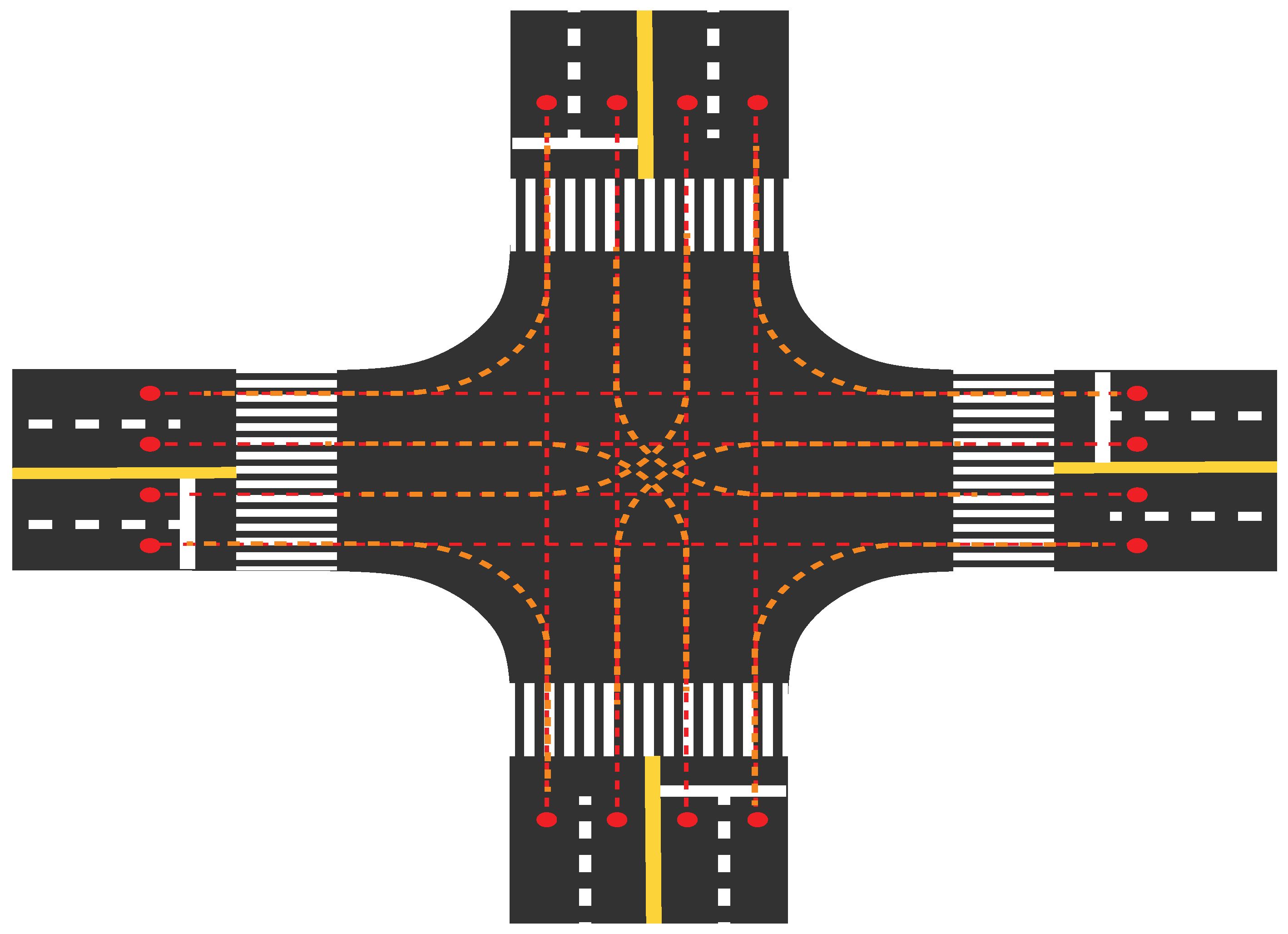
The road environment considered in this study is a four-lane bidirectional intersection, as illustrated in Figure 2. Following the principle of standardized safety testing, the road geometry, initial conditions, and scenario parameters are explicitly defined so that the same scenario configuration can be reproduced across repeated simulation runs. A situation is assumed in which an Ego vehicle and an NPC vehicle simultaneously enter the intersection. No commanded acceleration or deceleration is applied during scenario execution; therefore, each vehicle is intended to maintain its assigned constant speed unless its motion is affected by the simulated interaction or termination condition. Various driving patterns were defined with reference to the types of accidents that may occur at intersections [31]. The simulation map was configured with road-width and intersection-structure information, and each road segment was assigned a unique identifier. Because the OpenDRIVE road network used in this study does not provide all possible intersection connections, particularly U-turn connectivity, the generated scenarios are restricted to ST, LT, and RT maneuvers. Consequently, not all possible intersection accident configurations are represented in the present dataset.

3.1.2. OpenSCENARIO-Based Scenario Structure

In simulation, the map and scenario have complementary roles: the map defines the spatial structure in which vehicles move, while the scenario specifies vehicle behavior within that space. The map consists of predefined elements, and rendering methods and environmental factors (e.g., lighting, vegetation, structures, physics engine) vary across simulators. As these differences affect sensor data such as LiDAR and Radar, all experiments were conducted within a single simulator environment. OpenSCENARIO definitions used in this study follow v1.2 (https://www.asam.net/static_downloads/ASAM_OpenSCENARIO_V1.2.0_Model_Documentation/modelDocumentation/RenderedXsdOutput.html, accessed on 11 August 2026). The scenarios consist of four main components:

• Entity definition (Ego vehicle, NPC vehicle);
• Environment configuration and entity initial state;
• Scenario action definition;
• Success and failure conditions.

Specifically, the Ego and NPC vehicles are defined, their initial positions and speeds are set, and the direction of travel is specified through the scenario. The scenario is considered successful if the Ego vehicle reaches the goal point within the time limit (30 s), and a failure if a collision with another object occurs or the goal is not reached within the time limit.

3.1.3. Scenario Types and Data Generation

Scenarios for straight (ST), left-turn (LT), and right-turn (RT) situations were constructed based on possible accident types at a four-lane bidirectional intersection [31]. Each logical scenario specifies the starting positions and travel directions of the Ego and NPC vehicles. In the training and validation configuration, both vehicles initially start 25 m from the intersection. Concrete scenarios were generated by combining temporal, initial-speed, and environmental parameters with lane-level variations of the road network. This procedure produced 10,976 ST, 5488 LT, and 784 RT simulation instances, which were subsequently divided into training and validation subsets.

The test dataset was generated separately using a modified parameter configuration shared across all scenario types. As summarized in

Table 1. Parameter configurations for generating the training and validation data and the separately generated test data. Environmental values are shown as paired road friction coefficient ($\mu$) and visibility range (V).

Category	Parameter	Training and Validation	Test
Time	Time of day	06:00, 14:00, 19:00, 22:00	03:00, 12:00, 23:00
Initial Speed	Ego speed	8.33–16.67 m/s; step: ≈1.39 m/s (5 km/h)	8.33–16.67 m/s; step: ≈2.78 m/s (10 km/h)
	NPC speed	8.33–16.67 m/s; step: ≈1.39 m/s (5 km/h)	8.33–16.67 m/s; step: ≈2.78 m/s (10 km/h)
Environment	Rain	$\mu =0.7$, $V=200$ m	$\mu =0.8$, $V=250$ m
	Snow	$\mu =0.4$, $V=200$ m	$\mu =0.6$, $V=150$ m
	Sunny	$\mu =1.0$, $V=5000$ m	$\mu =1.0$, $V=4000$ m
	Fog	$\mu =1.0$, $V=50$ m	$\mu =1.0$, $V=80$ m

, test scenarios use different times of day and modified road friction and visibility settings. The initial-speed range remains unchanged, while the sampling interval increases from approximately 5 to 10 km/h. The test dataset therefore evaluates classification under new temporal and environmental parameter settings within the same scenario generation framework, with some individual parameter values shared with the training and validation configuration.

For both dataset configurations, environmental parameters are specified as coupled sets, preserving the prescribed combination of precipitation type, road friction, and visibility for each condition. These sets are combined with temporal and initial-speed parameters and the lane-level configurations of each logical scenario.

3.1.4. Data Labeling

The generated data were assigned trajectory and disturbance labels. Trajectory labels identify the Ego vehicle maneuver as straight (ST), left-turn (LT), or right-turn (RT). Following the conceptual categorization of perception, decision-making, and control discussed in Section 2, the present study uses perception and decision disturbances as quantitative classification targets. These labels characterize scenario conditions and simulation outcomes rather than directly diagnosing failures in individual autonomous driving components. The same labeling criteria are applied to the training, validation, and separately generated test datasets.

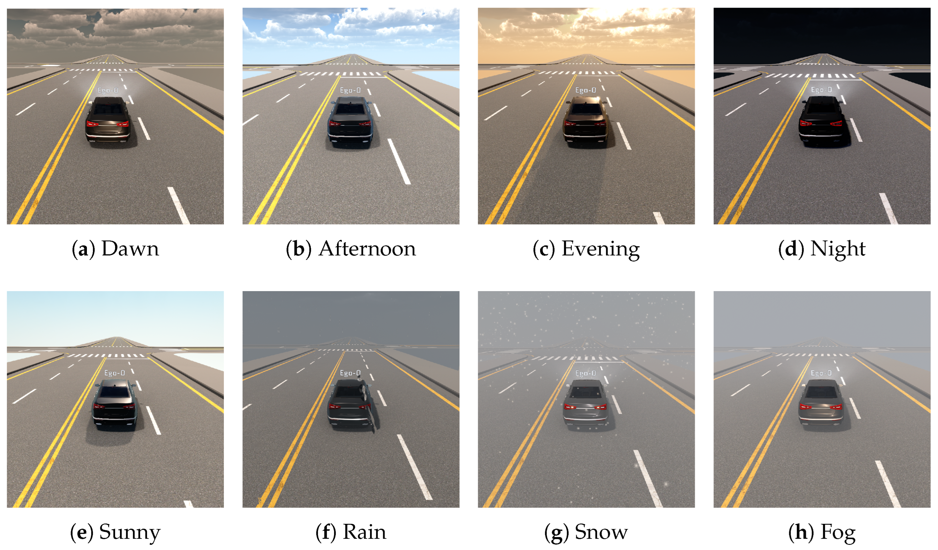
For perception disturbances, environmental conditions associated with potential sensor-performance degradation are used as labeling criteria [17,18,19,20,21,22,23,28]. The binary label is set to 1 when a scenario contains adverse weather (rain, snow, or fog) or a designated low-illumination condition, and to 0 otherwise. The low-illumination settings correspond to 06:00 and 22:00 in the training and validation configuration and 03:00 and 23:00 in the test configuration. Thus, the labeling rule remains consistent across datasets despite differences in their parameter values. Representative environmental conditions are illustrated in Figure 3.

For decision disturbances, an explicit event-based criterion is used: the binary label is set to 1 when a collision between the Ego and NPC vehicles occurs during simulation, and to 0 otherwise. The present study uses the Ego trajectory as the motion input without explicitly incorporating relative-motion features between vehicles into the trajectory encoder. Collision occurrence provides an observable outcome for labeling, while the Ego trajectory represents the vehicle motion used for classification. The label therefore identifies a collision-related outcome rather than directly quantifying pre-collision interaction risk. To characterize interactions with other vehicles, surrogate safety measures such as TTC, headway, TCPA, and DCPA can be considered using relative-state information and appropriate thresholds or risk-mapping rules. These supplementary indicators are summarized in Appendix A as possible extensions for pre-collision risk analysis.

For control disturbances, the scenario configuration includes the road-friction parameter, which can influence vehicle response to driving commands. However, the available data are insufficient to establish a reliable relationship between the specified friction values and the occurrence of a control disturbance. Road friction alone is therefore not used as a labeling criterion in the present experiments. It is retained as an environmental parameter, while control disturbances remain part of the conceptual categorization and are excluded from classifier training and quantitative evaluation. Each scenario is consequently represented by a joint label tuple,

$$\mathbf{y}=\left(y_{\mathrm{traj}},y_{\mathrm{perc}},y_{\mathrm{dec}}\right),$$

(1)

where $y_{\mathrm{traj}}\in \{\mathrm{ST},\mathrm{LT},\mathrm{RT}\}$ identifies the Ego maneuver, and $y_{\mathrm{perc}},y_{\mathrm{dec}}\in \{0, 1\}$ describe the perception-related condition and collision-related outcome, respectively. This representation distinguishes scenarios that share the same maneuver but differ in disturbance labels. It provides a common basis for grouping and comparing simulation cases across both behavioral and disturbance-related categories.

3.1.5. Analysis of Simulation Data

Various driving data were collected by executing the generated scenarios through simulation. Key features of the acquired data are summarized in

Table 2. Major Features in the Driving Trajectory Dataset.

Feature	Type/Unit
Time	s (sec)
Entity	String
Velocity X (entity coordinate)	km/h
Velocity Y (entity coordinate)	km/h
Velocity Z (entity coordinate)	km/h
Acceleration X (entity coordinate)	m/s2
Acceleration Y (entity coordinate)	m/s2
Acceleration Z (entity coordinate)	m/s2

. Variables such as position coordinates, velocity, and acceleration directly reflect the vehicle’s driving state and play an important role in driving behavior analysis.

The motion representation uses velocity and acceleration rather than absolute position to describe vehicle behavior without directly encoding its location within the simulation map. Position data remain available in the simulation logs but are not included in the Autoencoder input. The simulation data were collected at 50 Hz.

3.2. SinD Dataset

This section describes the SinD dataset used to train the variable-length Autoencoders, including the dataset structure, preprocessing procedures, and statistical properties.

3.2.1. SinD Dataset Overview

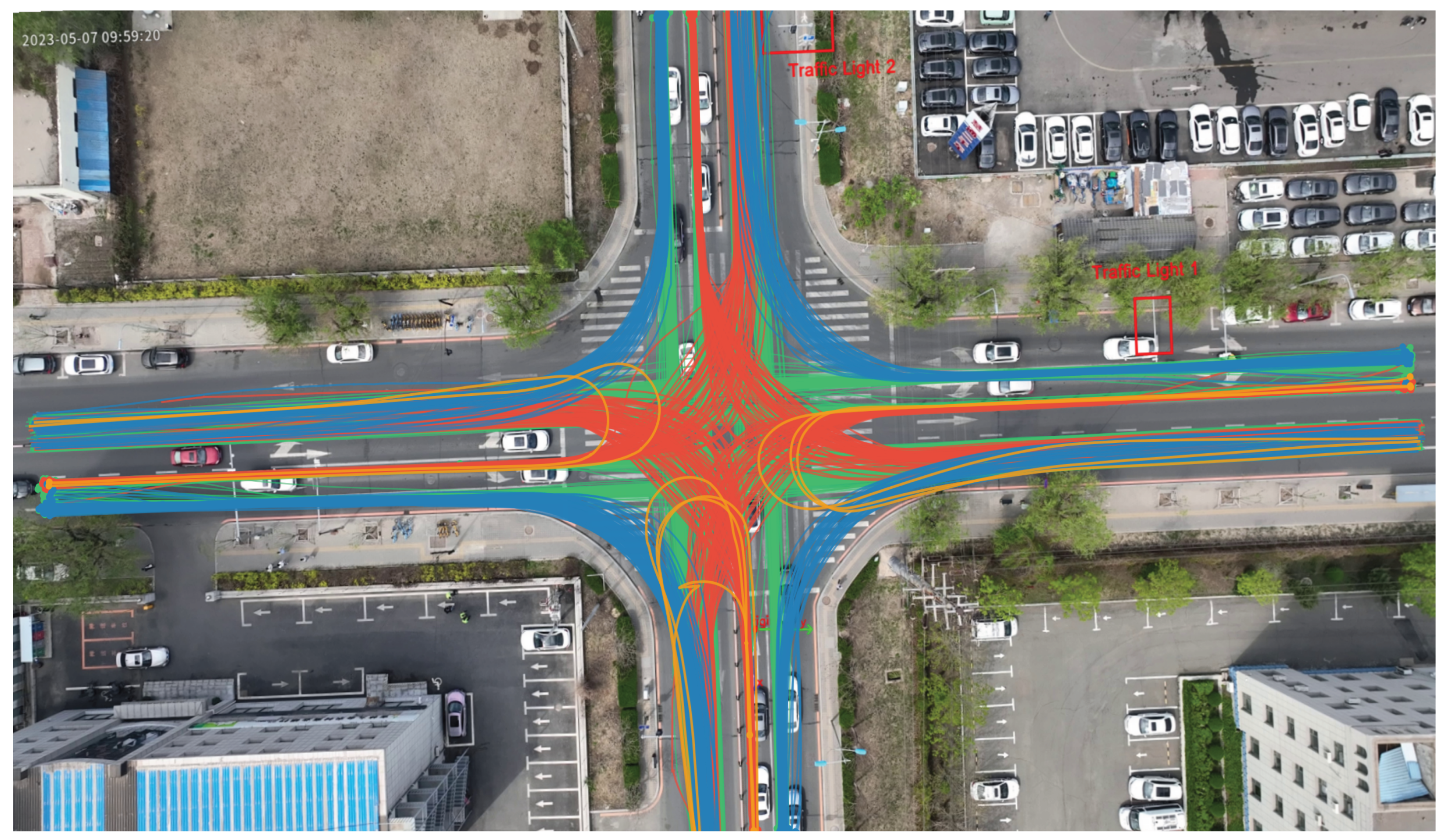
Our previous work classified vehicle trajectories into seven classes using simulation-generated data [12]. While this approach enabled classification within the evaluated simulation scenarios, its applicability to real-world trajectory data was not established. In the present study, the SinD dataset is used to train the trajectory Autoencoders using observations collected from real intersection environments [51]. SinD provides positional information for vehicles and other road users extracted from drone recordings at urban intersections in China, as illustrated in Figure 4. These observations introduce real-world motion variations into representation learning, without implying generalization to driving environments beyond those evaluated in this study.

3.2.2. Data Preprocessing

SinD includes a variety of intersection structures with different geometric configurations across locations. Most data was collected in intersection environments, with vehicle behaviors including straight driving, left turns, right turns, and U-turns. The dataset also includes diverse traffic participants such as trucks and motorcycles, as well as pedestrians. The following preprocessing steps were applied to align SinD with the simulation data format:

• Vehicle objects were isolated and pedestrian and other non-vehicle data were excluded.
• The temporal resolution was resampled to 50 Hz via interpolation to match the simulation data, ensuring temporal consistency between the two datasets.
• Time-series data were separated per vehicle and U-turn (UT) data were excluded as the simulation map does not define U-turn routing.
• Unlike the simulation data, SinD does not contain the environmental scenario attributes or explicit simulation collision outcomes used to define the perception- and decision-disturbance labels in this study. Therefore, SinD is used only for learning vehicle-motion representations and is not assigned disturbance labels.

3.3. Model Architecture

This section describes the model architecture and training procedure. The proposed method is based on a multimodal structure that independently encodes structural environmental information from the scenario file and vehicle motion information from simulation data, then combines them for classification.

3.3.1. Autoencoder-Based Variable-Length Time Series Encoding

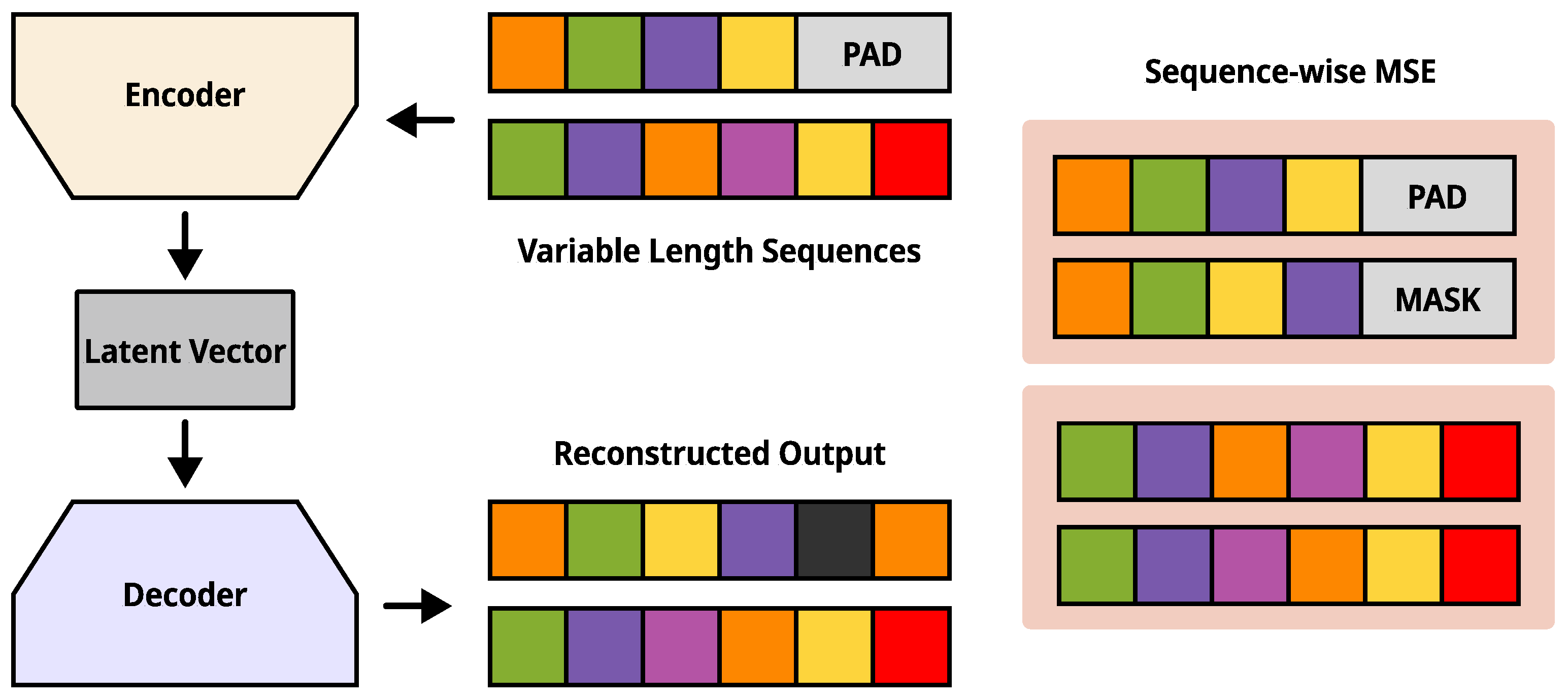
Autoencoders were used to learn compressed latent representations of vehicle motion at intersections [52,53]. The input consists of vehicle state time series from the SinD dataset, represented by six features at each time step: velocities ($ve{l}_x$, $ve{l}_y$, $ve{l}_z$) and accelerations ($ac{c}_x$, $ac{c}_y$, $ac{c}_z$) in the three coordinate directions [12,54]. The features were normalized using per-feature means and standard deviations obtained from the training subset, with the same statistics applied to the validation subset. A moving average with a window size of five was applied to smooth temporal fluctuations. To limit memory requirements, the maximum input sequence length was set to 15,000 time steps, corresponding to approximately five minutes at 50 Hz. Vehicle trajectories vary in duration across scenarios. The training pipeline processes sequences in mini-batches together with their valid lengths. A binary mask derived from these lengths excludes padded time steps from the reconstruction loss, so that only valid observations contribute to the reconstruction objective.

Six Autoencoder configurations were considered: Simple-AE, BiLSTM-AE, Stacked-AE, Transformer-AE, xLSTM-AE, and Mamba-AE. The first three employ conventional LSTM encoders, while the remaining configurations use Transformer, xLSTM, and Mamba temporal modeling components, respectively [47,49,50]. All models follow the Encoder–Bottleneck–Decoder structure illustrated in Figure 5. The encoder maps the input sequence to a fixed-dimensional latent representation, and the decoder reconstructs the sequence from this representation. After training, the encoder provides vehicle-motion features for downstream scenario classification.

The reconstruction objective is the masked mean squared error,

$${\mathrm{MSE}}_{\mathrm{masked}}={\displaystyle \frac{{\sum }_{b,t,d}{m}_{b,t}{\left(x_{b,t,d}-{\widehat{x}}_{b,t,d}\right)}^2}{D{\sum }_{b,t}{m}_{b,t}}},$$

(2)

where $x_{b,t,d}$ and ${\widehat{x}}_{b,t,d}$ denote the observed and reconstructed values of feature d at time step t in sequence b, respectively. The mask $m_{b,t}$ equals one for valid observations and zero for padding, and D is the feature dimensionality. All Autoencoder models were optimized for 300 epochs using AdamW with a learning rate of ${10}^{-3}$ and weight decay of ${10}^{-4}$.

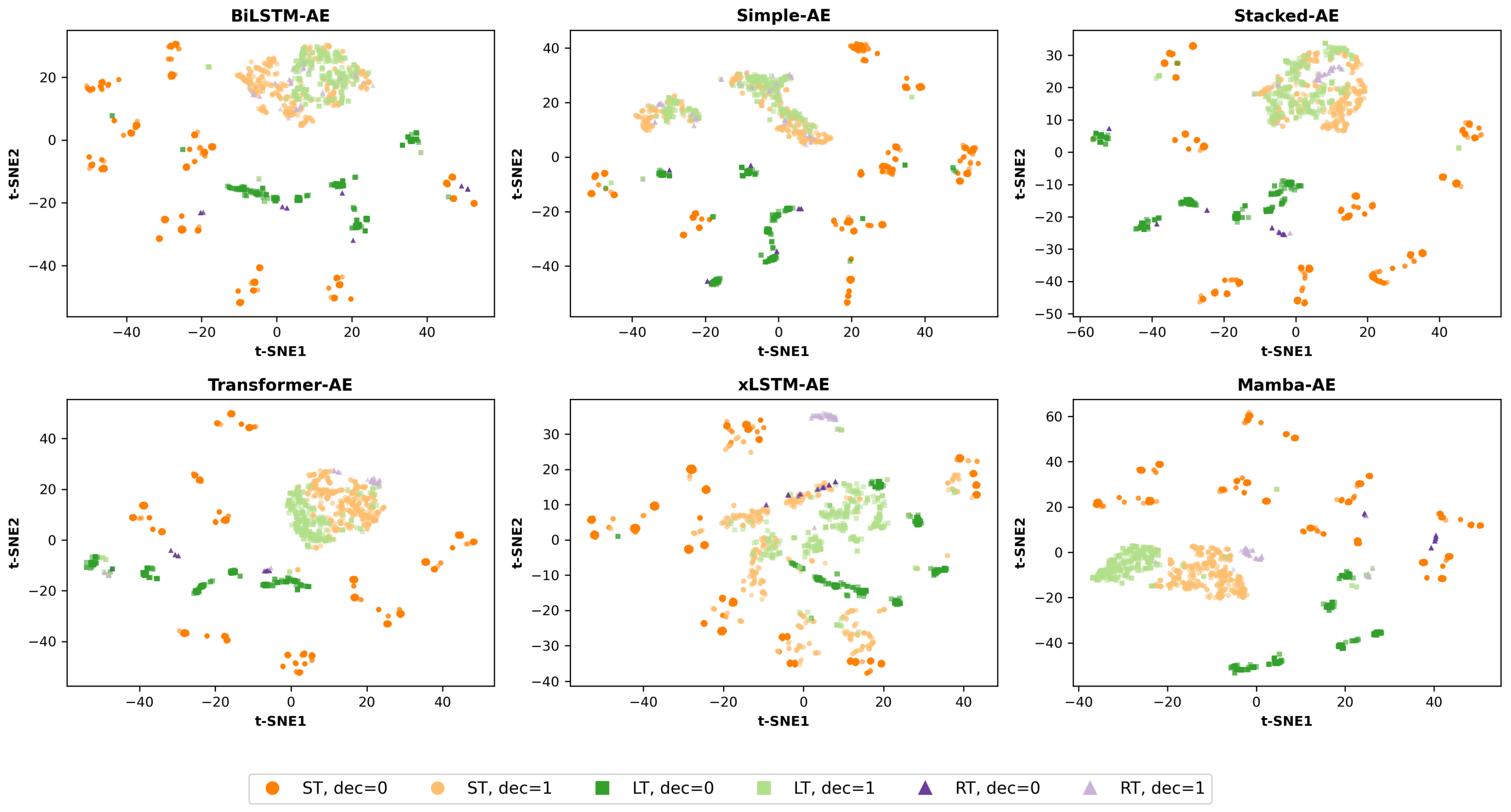
The learned latent representations were first processed using PCA for dimensionality reduction and then projected into two dimensions using t-SNE, as shown in Figure 6. Colors and marker shapes identify trajectory types, while darker and lighter shades distinguish the binary decision labels. The visualization provides a qualitative view of local grouping and overlap in the latent space. The t-SNE projections show local groups associated with trajectory types and decision labels. In several encoders, decision-0 samples form multiple compact groups, while decision-1 samples occupy regions with overlapping trajectory types. Mamba-AE shows comparatively distinct ST and LT groups among the decision-1 samples, although complete separation is not observed across all classes. These projections provide qualitative evidence of latent structure, but their two-dimensional grouping alone does not establish downstream classification performance. To complement the visual analysis,

Table 3. Domain distribution metrics between SinD and simulation data. The reference consists of standardized per-log summaries of velocity and acceleration features. Comparisons across representations are descriptive.

Representation	Domain Silhouette	MMD2
Log-summary reference	0.2112	0.3618
BiLSTM-AE	0.1739	0.2165
Simple-AE	0.1279	0.1821
Stacked-AE	0.2111	0.2368
Transformer-AE	0.2224	0.2376
xLSTM-AE	0.1525	0.1827
Mamba-AE	0.1826	0.2610

reports the SinD–simulation domain silhouette score and squared maximum mean discrepancy (MMD²). The silhouette score measures separation according to dataset membership, whereas MMD² measures discrepancy between the two distributions. These metrics characterize domain differences rather than trajectory- or decision-label separability.

All encoders produced positive domain silhouette scores, indicating that domain-related structure remains in the latent spaces. Several encoders yielded lower silhouette scores than the log-summary reference, while Stacked-AE remained nearly unchanged and Transformer-AE showed a slight increase. All six encoders also yielded lower reported MMD² values than the reference. These comparisons are descriptive because the log-summary vectors and learned representations differ in feature construction and dimensionality. Lower reported values do not independently establish domain alignment, preservation of task-relevant information, or improved cross-domain generalization. The downstream classification results provide the direct assessment of the representations’ utility within the evaluated scenario configurations.

3.3.2. Text Encoder Selection

OpenSCENARIO uses a structured XML-based format in which environmental conditions, entity definitions, initial states, and scenario actions are explicitly represented. Because the amount and structural complexity of this information increase with scenario complexity, the scenario file is converted into a machine-processable textual representation rather than manually reducing it to a small set of numerical attributes. In the proposed pipeline, the OpenSCENARIO file is parsed and serialized as a JSON string before text encoding. This preserves the hierarchical scenario information while providing a consistent input form for pre-trained text encoders.

Large generative language models could also be used for this purpose, but repeated scenario-level embedding would introduce substantial computational overhead. Therefore, pre-trained Transformer-based embedding models were selected to balance representation capability and computational cost. Four encoders with different model sizes and embedding dimensions were evaluated: EmbeddingGemma-300M, all-MiniLM-L6-v2, BGE-M3, and Qwen3-Embedding-0.6B. Their main characteristics are summarized in

Table 4. Text Encoders Used for Comparative Evaluation.

Model	Embedding Dim.	Parameters
EmbeddingGemma-300M	768	307.6M
all-MiniLM-L6-v2	384	22.7M
BGE-M3	1024	567.8M
Qwen3-Embedding-0.6B	1024	595.8M

. The encoders are used as pre-trained feature extractors, and their output embeddings are subsequently combined with the trajectory latent vectors produced by the Autoencoders.

3.3.3. Full Model Architecture

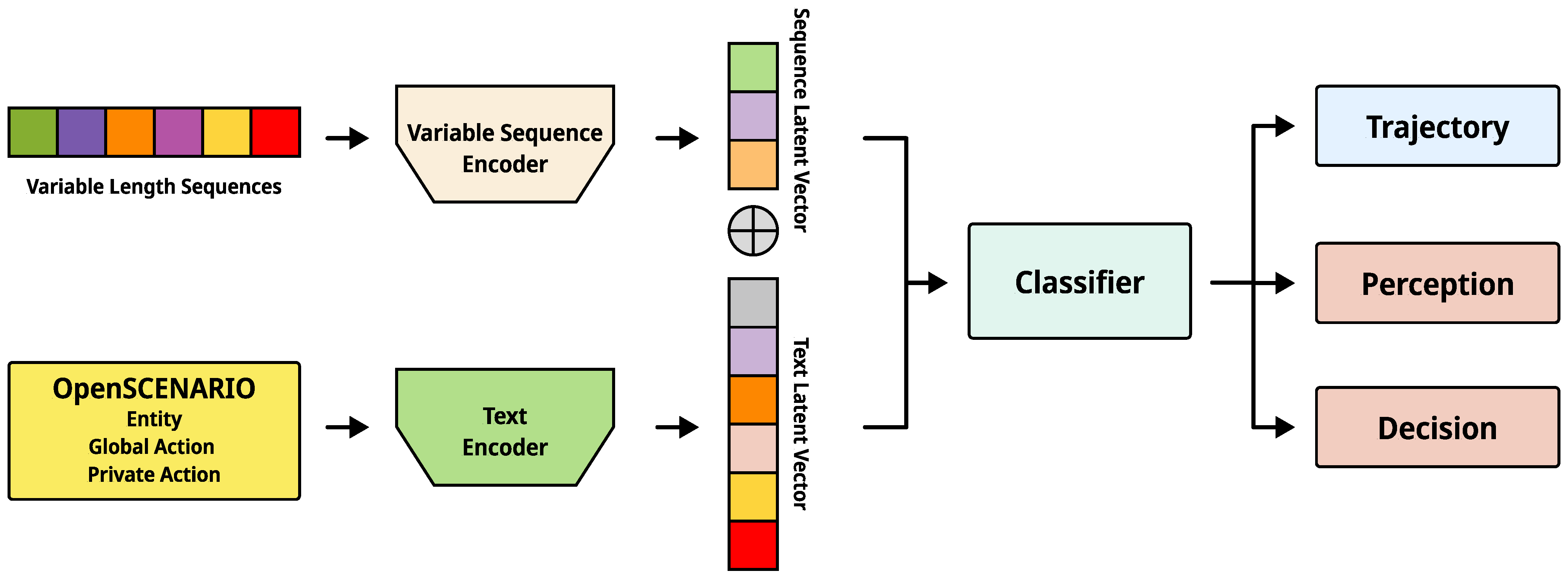
The overall model integrates a pre-trained AE and a pre-trained text encoder to perform multi-task classification of intersection scenarios. Vehicle motion features are extracted by the AE encoder, yielding a 64-dimensional latent vector from the Ego vehicle’s velocity and acceleration time series. Scenario structural features are obtained by parsing the OpenSCENARIO file, serializing the structured information as a JSON string, and encoding it with one of the four pre-trained text encoders described in Section 3.3.1. The final classifier input is formed by concatenating the trajectory latent vector and the text embedding. All 24 combinations (6 trajectory AEs × 4 text encoders) are independently trained and compared. The overall processing pipeline is illustrated in Figure 7.

The classifier consists of a shared MLP backbone and three task-specific heads. The backbone combines scenario context and observed vehicle motion by processing the concatenated features through fully connected layers with LayerNorm, ReLU, and Dropout. The task-specific heads predict trajectory type (ST/LT/RT), perception disturbance, and decision disturbance, forming the joint scenario label defined in Section 3.1.4. Control disturbance is excluded from the prediction targets, consistent with the labeling scope. Per-task metrics evaluate the individual outputs, while Full Match Accuracy measures whether the complete scenario label is predicted correctly.

Each task loss is defined using cross-entropy:

$${\mathcal{L}}_{\mathrm{task}}=-{\displaystyle \sum _{c=1}^C}{y}_{c}log{\widehat{p}}_c,$$

(3)

where $y_c$ denotes the ground-truth label for class c and ${\widehat{p}}_c$ denotes the predicted probability for class c.

For the fixed-weight configuration, the relative task weights are assigned as $1:0.5:0.5$ for trajectory, perception disturbance, and decision disturbance, respectively. The total loss is therefore defined as

$${\mathcal{L}}_{\mathrm{fixed}}={\mathcal{L}}_{\mathrm{traj}}+{\displaystyle \frac{1}{2}}\left({\mathcal{L}}_{\mathrm{perc}}+{\mathcal{L}}_{\mathrm{dec}}\right).$$

(4)

For the uncertainty-weighted configuration, each task is assigned a learnable log-variance parameter

$$s_i=log{\sigma }_i^2,i\in \{\mathrm{traj},\mathrm{perc},\mathrm{dec}\}.$$

(5)

For numerical stability, the log-variance is clipped to the interval $[-2, 2]$:

$${\tilde{s}}_i=clip(s_i,-2, 2).$$

(6)

The uncertainty-weighted objective is defined as

$${\mathcal{L}}_{\mathrm{unc}}=\sum _{i\in \{\mathrm{traj},\mathrm{perc},\mathrm{dec}\}}\left[exp(-{\tilde{s}}_i){\mathcal{L}}_i+{\tilde{s}}_i\right],$$

(7)

Here, ${\mathcal{L}}_i$ denotes the loss of the corresponding task. The factor $exp(-{\tilde{s}}_i)$ determines the task weight from the clipped log-variance, while the additive ${\tilde{s}}_i$ term regularizes the learned weighting. The classifier and log-variance parameters were optimized jointly using AdamW. The quantitative evaluation considered trajectory type, perception disturbance, and decision disturbance. The simulation dataset was stratified into training and validation subsets according to trajectory type and decision-disturbance labels, and the same split was used for all model configurations.

4. Results

We evaluate the proposed framework across 24 combinations of four text encoders (EmbeddingGemma, MiniLM, BGE-M3, and Qwen-Emb) and six trajectory autoencoder structures (BiLSTM-AE, Simple-AE, Stacked-AE, Transformer-AE, xLSTM-AE, and Mamba-AE). Classification performance is assessed on trajectory type (ST, LT, or RT), perception disturbance, and decision disturbance using per-task accuracy, trajectory macro-averaged F1, and Full Match Accuracy. Full Match Accuracy requires simultaneous correctness for all three labels. The test set contains 3840 samples, including 3520 perception-positive and 320 perception-negative samples. Predicting every sample as perception-positive yields an accuracy of 0.9167 and a positive-class F1 score of 0.9565. These values therefore serve as reference baselines and do not, by themselves, demonstrate discrimination between the two perception classes. Binary F1 values for perception and decision are positive-class F1 scores, whereas trajectory F1 is the macro-averaged F1 over ST, LT, and RT.

The main analysis focuses on the separately generated test dataset. Reported validation results are included to contextualize performance under the parameter configuration used for training, with detailed validation tables provided in Appendix B. The evaluation addresses three questions: how accurately the framework predicts individual targets and complete scenario labels; how encoder selection and task weighting affect these predictions; and how performance changes under modified scenario parameters and removal of either input modality. The following analyses therefore consider classification performance, configuration sensitivity, and input contributions within the integrated framework.

4.1. Fixed Task Weighting

Classification performance under fixed task weighting is presented in

Table 5. Test classification performance with fixed task weighting. F1 denotes trajectory macro F1; FM denotes Full Match Accuracy. Bold values identify the highest reported score in each column.

Text Encoder	Trajectory AE	Traj. Acc.	F1	Perc. Acc.	Dec. Acc.	FM
EmbeddingGemma	BiLSTM-AE	0.8354	0.8555	0.9167	0.9992	0.7641
EmbeddingGemma	Simple-AE	0.9583	0.9339	0.9167	0.9990	0.8771
EmbeddingGemma	Stacked-AE	0.7474	0.7554	0.9167	0.9997	0.6849
EmbeddingGemma	Transformer-AE	0.8276	0.8212	0.9167	0.9844	0.7435
EmbeddingGemma	xLSTM-AE	0.6193	0.3471	0.9167	0.7365	0.4081
EmbeddingGemma	Mamba-AE	0.9997	0.9990	0.9167	0.9992	0.9156
MiniLM	BiLSTM-AE	0.8714	0.7748	0.6086	0.9997	0.5414
MiniLM	Simple-AE	0.9792	0.9660	0.2953	0.9997	0.2917
MiniLM	Stacked-AE	0.9201	0.9357	0.8096	0.9997	0.7516
MiniLM	Transformer-AE	0.8805	0.9071	0.8979	0.9979	0.7893
MiniLM	xLSTM-AE	0.6557	0.5344	0.8516	0.9352	0.5169
MiniLM	Mamba-AE	0.9997	0.9990	0.5721	0.9992	0.5719
BGE-M3	BiLSTM-AE	0.9724	0.9692	0.7544	1.0000	0.7310
BGE-M3	Simple-AE	0.9763	0.9692	0.7940	0.9990	0.7729
BGE-M3	Stacked-AE	0.8740	0.8528	0.8398	0.9990	0.7312
BGE-M3	Transformer-AE	0.8807	0.9127	0.8323	0.9948	0.7299
BGE-M3	xLSTM-AE	0.6625	0.5289	0.8008	0.8445	0.4792
BGE-M3	Mamba-AE	0.9995	0.9980	0.8674	0.9990	0.8659
Qwen-Emb	BiLSTM-AE	0.9641	0.9598	0.9167	1.0000	0.8831
Qwen-Emb	Simple-AE	0.9641	0.9637	0.9167	0.9997	0.8833
Qwen-Emb	Stacked-AE	0.8823	0.8596	0.9167	0.9987	0.8078
Qwen-Emb	Transformer-AE	0.8339	0.7573	0.9167	0.9984	0.7625
Qwen-Emb	xLSTM-AE	0.6594	0.5284	0.9167	0.8854	0.5357
Qwen-Emb	Mamba-AE	0.9997	0.9990	0.9167	0.9997	0.9161

. Mamba-AE achieved the strongest trajectory classification performance across text encoder pairings, with consistently high trajectory accuracy and macro F1. Perception and decision performance varied more substantially across encoder pairings, indicating that joint performance depends on the interaction between the text and trajectory representations. Under fixed weighting, Qwen-Emb with Mamba-AE achieved the highest Full Match Accuracy of 0.9161. Although this configuration obtained near-perfect trajectory and decision scores, its perception accuracy matched the majority-class baseline. The Full Match result therefore indicates high simultaneous label agreement on the evaluated test distribution, but does not establish balanced discrimination of perception-positive and perception-negative scenarios.

4.2. Uncertainty-Based Task Weighting

Uncertainty-based weighting adjusts the contribution of each task through learnable log-variance parameters.

Table 6. Test classification performance with uncertainty-based task weighting. F1 denotes trajectory macro F1; FM denotes Full Match Accuracy. Bold values identify the highest reported score in each column.

Text Encoder	Trajectory AE	Traj. Acc.	F1	Perc. Acc.	Dec. Acc.	FM
EmbeddingGemma	BiLSTM-AE	0.8510	0.8745	0.9167	0.9997	0.7784
EmbeddingGemma	Simple-AE	0.9372	0.8802	0.9167	1.0000	0.8594
EmbeddingGemma	Stacked-AE	0.7672	0.7762	0.9167	0.9990	0.7008
EmbeddingGemma	Transformer-AE	0.8135	0.8115	0.9164	0.9792	0.7263
EmbeddingGemma	xLSTM-AE	0.6440	0.5258	0.9159	0.7602	0.4315
EmbeddingGemma	Mamba-AE	0.9995	0.9980	0.9167	0.9992	0.9154
MiniLM	BiLSTM-AE	0.8622	0.8913	0.2690	0.9997	0.2195
MiniLM	Simple-AE	0.9818	0.9787	0.6000	0.9997	0.5888
MiniLM	Stacked-AE	0.8919	0.8957	0.4076	0.9997	0.3773
MiniLM	Transformer-AE	0.8620	0.8773	0.8930	0.9961	0.7693
MiniLM	xLSTM-AE	0.6628	0.5478	0.8286	0.8729	0.5255
MiniLM	Mamba-AE	0.9995	0.9980	0.3052	0.9990	0.3036
BGE-M3	BiLSTM-AE	0.9146	0.9287	0.8159	1.0000	0.7531
BGE-M3	Simple-AE	0.9792	0.9760	0.8422	0.9997	0.8224
BGE-M3	Stacked-AE	0.8901	0.9090	0.8609	0.9990	0.7643
BGE-M3	Transformer-AE	0.8771	0.9081	0.7073	0.9958	0.6174
BGE-M3	xLSTM-AE	0.6924	0.6421	0.7370	0.8375	0.4401
BGE-M3	Mamba-AE	0.9995	0.9980	0.8578	0.9990	0.8562
Qwen-Emb	BiLSTM-AE	0.9682	0.9664	0.9167	1.0000	0.8867
Qwen-Emb	Simple-AE	0.9680	0.9660	0.9167	0.9997	0.8870
Qwen-Emb	Stacked-AE	0.8240	0.8172	0.9167	0.9987	0.7570
Qwen-Emb	Transformer-AE	0.8643	0.8948	0.9167	0.9802	0.7732
Qwen-Emb	xLSTM-AE	0.6667	0.5556	0.9167	0.7185	0.4190
Qwen-Emb	Mamba-AE	0.9995	0.9980	0.9167	1.0000	0.9161

shows the corresponding test results. The best Full Match Accuracy was 0.9161, achieved by Qwen-Emb with Mamba-AE, while performance varied across other text–trajectory encoder pairings. Compared with fixed weighting, uncertainty-based weighting did not provide a consistent improvement in Full Match Accuracy. Its effect depended on the encoder pairing and task: some configurations improved trajectory F1, whereas disturbance accuracy or Full Match Accuracy decreased. These results indicate that task weighting and encoder selection should be considered jointly.

4.3. Encoder-Wise Comparison

To compare architectures independently of a single text encoder pairing,

Table 7. Mean classification performance by trajectory encoder and text encoder under fixed and uncertainty-based weighting. Each trajectory encoder mean is computed over four text encoders; each text encoder mean is computed over six trajectory encoders. Trajectory F1 is macro F1 over ST/LT/RT; perception and decision F1 are positive-class F1 scores. Bold values identify the highest reported score in each column.

Encoder	Weighting	Trajectory		Perception		Decision		FM
		Acc.	F1	Acc.	F1	Acc.	F1
BiLSTM-AE	Fixed	0.9108	0.8898	0.7991	0.8737	0.9997	0.9996	0.7299
	Uncertainty	0.8990	0.9152	0.7296	0.7847	0.9999	0.9998	0.6594
Simple-AE	Fixed	0.9695	0.9582	0.7307	0.7906	0.9993	0.9991	0.7063
	Uncertainty	0.9665	0.9502	0.8189	0.8868	0.9998	0.9997	0.7894
Stacked-AE	Fixed	0.8559	0.8509	0.8707	0.9269	0.9993	0.9990	0.7439
	Uncertainty	0.8433	0.8495	0.7755	0.8403	0.9991	0.9987	0.6499
Transformer-AE	Fixed	0.8557	0.8496	0.8909	0.9396	0.9939	0.9914	0.7563
	Uncertainty	0.8542	0.8729	0.8583	0.9162	0.9878	0.9831	0.7215
xLSTM-AE	Fixed	0.6492	0.4847	0.8714	0.9282	0.8504	0.7243	0.4850
	Uncertainty	0.6665	0.5678	0.8495	0.9133	0.7973	0.6780	0.4540
Mamba-AE	Fixed	0.9997	0.9988	0.8182	0.8840	0.9993	0.9990	0.8174
	Uncertainty	0.9995	0.9980	0.7491	0.8048	0.9993	0.9990	0.7479
EmbeddingGemma	Fixed	0.8313	0.7853	0.9167	0.9565	0.9530	0.9005	0.7322
	Uncertainty	0.8354	0.8110	0.9165	0.9564	0.9562	0.9099	0.7353
MiniLM	Fixed	0.8844	0.8528	0.6725	0.7609	0.9886	0.9825	0.5771
	Uncertainty	0.8767	0.8648	0.5506	0.6386	0.9779	0.9698	0.4640
BGE-M3	Fixed	0.8942	0.8718	0.8148	0.8880	0.9727	0.9554	0.7184
	Uncertainty	0.8921	0.8936	0.8035	0.8792	0.9718	0.9494	0.7089
Qwen-Emb	Fixed	0.8839	0.8447	0.9167	0.9565	0.9803	0.9699	0.7981
	Uncertainty	0.8818	0.8663	0.9167	0.9565	0.9495	0.9432	0.7732

reports the mean performance of each trajectory encoder across the four text encoders and of each text encoder across the six trajectory encoders. Mamba-AE achieved the highest mean trajectory accuracy, trajectory F1, and Full Match Accuracy under fixed weighting. Among text encoders, Qwen-Emb achieved the highest fixed-weight mean Full Match Accuracy. The results also show that the best individual pairing does not necessarily imply uniformly superior performance across all tasks.

4.4. Validation and Test Comparison

Table 8. Reported validation and test performance averaged over six trajectory encoders for each text encoder. All denotes the unweighted mean over all 24 encoder combinations. Perc. denotes perception accuracy and FM denotes Full Match Accuracy.

Text Encoder	Weighting	Perc. Val.	Perc. Test	FM Val.	FM Test
EmbeddingGemma	Fixed	1.0000	0.9167	0.9757	0.7322
EmbeddingGemma	Uncertainty	0.9996	0.9165	0.9416	0.7353
MiniLM	Fixed	0.9938	0.6725	0.9727	0.5771
MiniLM	Uncertainty	0.9471	0.5506	0.8986	0.4640
BGE-M3	Fixed	1.0000	0.8148	0.9758	0.7184
BGE-M3	Uncertainty	0.9732	0.8035	0.9217	0.7089
Qwen-Emb	Fixed	0.9574	0.9167	0.9393	0.7981
Qwen-Emb	Uncertainty	0.9088	0.9167	0.8543	0.7732
All	Fixed	0.9878	0.8302	0.9659	0.7064
All	Uncertainty	0.9572	0.7968	0.9041	0.6704

summarizes the reported validation and test performance, averaged over the six trajectory encoders for each text encoder. The validation subset was drawn from the scenario collection generated under the training parameter configuration, whereas the test dataset was generated separately using modified times of day and environmental settings. Detailed validation results for all encoder combinations are provided in Appendix B.

Validation perception accuracy was generally higher than test accuracy under both weighting strategies. High performance within the training parameter configuration therefore did not consistently extend to the modified test configuration. The magnitude of this difference depended on the encoder pairing, and not every configuration showed a decrease. The corresponding Full Match results also indicate that strong validation performance did not ensure equally high simultaneous classification accuracy on the test set. Perception labels are defined using weather and time-of-day conditions described in the scenario text. The validation–test differences show that performance under the training parameter configuration did not consistently extend to the modified test configuration. However, the comparison does not isolate the effects of individual parameter changes or identify text-encoder representation quality as the cause. Differences in class composition and scenario coverage may also influence aggregate accuracy. The results should therefore be interpreted as performance under a changed test configuration rather than as a controlled estimate of the effect of weather or time-of-day changes alone.

4.5. Latent-Vector Ablation

To examine the contribution of the two modalities, the trained checkpoints were evaluated after setting either the text latent vector or the trajectory latent vector to zero.

Table 9. Latent-vector ablation results averaged over four text encoder pairings. M: full multimodal input; ZT: text latent vector set to zero; ZR: trajectory latent vector set to zero. Bold values identify the highest reported score in each column. All reported values are accuracies.

Weighting	Trajectory AE	Traj. M	Traj. ZT	Perc. M	Perc. ZR	Dec. M	Dec. ZR
Fixed	BiLSTM-AE	0.9108	0.5033	0.7991	0.8906	0.9997	0.3952
Fixed	Simple-AE	0.9695	0.7201	0.7307	0.8411	0.9993	0.3555
Fixed	Stacked-AE	0.8559	0.3831	0.8707	0.9167	0.9993	0.3555
Fixed	Transformer-AE	0.8557	0.4198	0.8909	0.9193	0.9939	0.3555
Fixed	xLSTM-AE	0.6492	0.6001	0.8714	0.9167	0.8504	0.3555
Fixed	Mamba-AE	0.9997	0.9997	0.8182	0.7552	0.9993	0.6445
Uncertainty	BiLSTM-AE	0.8990	0.3900	0.7296	0.8086	0.9999	0.3555
Uncertainty	Simple-AE	0.9665	0.6565	0.8189	0.9232	0.9998	0.3555
Uncertainty	Stacked-AE	0.8433	0.3762	0.7755	0.9167	0.9991	0.3555
Uncertainty	Transformer-AE	0.8542	0.4422	0.8583	0.8737	0.9878	0.3555
Uncertainty	xLSTM-AE	0.6665	0.6133	0.8495	0.8737	0.7973	0.3555
Uncertainty	Mamba-AE	0.9995	0.9994	0.7491	0.7005	0.9993	0.6445

reports the results averaged over the four text encoder pairings. These experiments measure input dependence within the trained multimodal classifier and are not comparisons with separately trained unimodal models. Removing the text latent vector substantially reduced trajectory accuracy for most encoders, whereas Mamba-AE retained nearly the same trajectory accuracy. Removing the trajectory latent vector consistently reduced decision accuracy, indicating that the decision heads relied strongly on trajectory information. Perception accuracy changed less consistently, demonstrating that the contribution of each modality was task- and encoder-dependent.

The results indicate task-dependent use of the two representations. In particular, trajectory information was important for decision disturbance classification, while the effect of text and trajectory removal on perception classification varied across encoder structures. Because these are zero-vector evaluations of already trained multimodal classifiers, they measure input dependence rather than the standalone performance of a newly trained unimodal model.

5. Conclusions

This section summarizes the main findings of the proposed multimodal scenario classification framework and discusses its limitations and future research directions.

5.1. Summary of Experimental Results

This study presented an integrated framework for classifying intersection scenarios through a joint description of vehicle maneuver, perception-related conditions, and collision-related outcomes. By combining OpenSCENARIO text embeddings with SinD-trained Ego-motion representations, the framework produces three classification outputs within a common multi-task pipeline. The evaluation across 24 encoder combinations and two weighting strategies showed that encoder selection affects both individual-task and joint performance. Qwen-Emb combined with Mamba-AE achieved the highest Full Match Accuracy of 0.9161, while uncertainty-based weighting did not consistently improve the results. Perception classification remained a limiting factor, demonstrating the importance of examining individual targets alongside the complete scenario label. The validation–test comparison and latent-vector ablations further characterized the framework’s behavior. High validation performance did not consistently extend to modified test parameters, and the contribution of each modality differed across tasks and encoder configurations. In particular, removing trajectory information substantially reduced decision-label classification performance, whereas Mamba-AE retained high trajectory accuracy after text removal. These findings establish the evaluated performance and input dependence of the proposed classification pipeline within the considered scenario family. The framework provides a basis for organizing simulation cases by both maneuver and disturbance labels, with broader scenario coverage and additional labeling criteria remaining directions for further development.

The proposed classification framework could support decision-making in digital twin-based autonomous driving validation by organizing simulated scenarios according to vehicle maneuvers, perception-related conditions, and collision-related outcomes. These joint labels provide a basis for retrieving comparable cases, examining the coverage of evaluated scenario categories, and selecting cases for further review. In this role, the framework provides scenario-level information for validation planning and analysis. Integration with an operational digital twin and assessment of its benefits to validation workflows remain to be investigated.

5.2. Limitations and Future Work

Several limitations remain in the current framework. First, the simulation dataset is generated from a constrained intersection environment with predefined vehicle behaviors and environmental conditions. Although this setup supports systematic scenario generation and reproducible evaluation, some classification targets may be easier to distinguish than in more diverse driving environments. Expanding the dataset to cover additional road geometries, maneuvers, and traffic participants, including lane changes, U-turns, roundabouts, and pedestrian interactions, would enable a broader assessment of the framework. Second, perception classification showed differences between validation and test performance under modified temporal and environmental settings. High validation accuracy therefore did not consistently indicate reliable classification under new parameter configurations. Further investigation should examine the representation of weather and illumination information, broaden environmental coverage, and assess performance using class-wise metrics alongside overall accuracy. Third, the decision-disturbance label is based on collision occurrence and therefore captures an interaction outcome rather than the severity of pre-collision risk. The current motion representation also uses only the Ego trajectory, without explicitly modeling relative motion between vehicles. Incorporating surrounding-vehicle trajectories and continuous safety indicators, such as TTC, headway, TCPA, and DCPA, could support more detailed interaction analysis and decision-disturbance labeling. Fourth, control disturbances were excluded from classifier training and quantitative evaluation. Although road friction is specified in the scenario configuration, the available data are insufficient to establish a reliable relationship between friction values and the occurrence of a control disturbance. Developing and validating control-disturbance labeling criteria will require additional vehicle-dynamics information and control-performance indicators, including tracking error and lateral stability. Finally, evaluation on larger and more diverse datasets, together with repeated runs, would help assess the robustness and performance variability of the encoder combinations and task-weighting strategies. Domain adaptation and joint representation learning with real-world and simulation data also warrant investigation to address the remaining distributional differences. These extensions will help determine the framework’s applicability beyond the scenario configurations evaluated in this study.

References

1. Chen, W.; Li, A.; Jiang, H. Risk Assessment of Roundabout Scenarios in Virtual Testing Based on an Improved Driving Safety Field. Sensors 2024, 24, 5539. [Google Scholar] [CrossRef] [Scilit]
2. Thal, S.; Wallis, P.; Henze, R.; Hasegawa, R.; Nakamura, H.; Kitajima, S.; Abe, G. Towards Realistic, Safety-Critical and Complete Test Case Catalogs for Safe Automated Driving in Urban Scenarios. In Proceedings of the 2023 IEEE Intelligent Vehicles Symposium (IV); IEEE: New York, NY, USA, 2023; pp. 1–8. [Google Scholar] [CrossRef] [Scilit]
3. Barabás, I.; Todoruţ, A.; Cordoş, N.; Molea, A. Current Challenges in Autonomous Driving. IOP Conf. Ser. Mater. Sci. Eng. 2017, 252, 012096. [Google Scholar] [CrossRef] [Scilit]
4. ISO 26262-1:2018; Road Vehicles—Functional Safety. International Organization for Standardization: Geneva, Switzerland, 2018. Available online: https://www.iso.org/standard/68383.html (accessed on 23 September 2026).
5. De Gelder, E.; Manders, J.; Grappiolo, C.; Paardekooper, J.P.; Den Camp, O.O.; De Schutter, B. Real-world scenario mining for the assessment of automated vehicles. In Proceedings of the 2020 IEEE 23rd International Conference on Intelligent Transportation Systems (ITSC); IEEE: New York, NY, USA, 2020; pp. 1–8. [Google Scholar]
6. Zhang, X.; Tao, J.; Tan, K.; Törngren, M.; Sánchez, J.M.G.; Ramli, M.R.; Tao, X.; Gyllenhammar, M.; Wotawa, F.; Mohan, N.; et al. Finding critical scenarios for automated driving systems: A systematic mapping study. IEEE Trans. Softw. Eng. 2022, 49, 991–1026. [Google Scholar] [CrossRef] [Scilit]
7. Dosovitskiy, A.; Ros, G.; Codevilla, F.; Lopez, A.; Koltun, V. CARLA: An Open Urban Driving Simulator. In Proceedings of the 1st Annual Conference on Robot Learning; PMLR: Cambridge, MA, USA, 2017; pp. 1–16. [Google Scholar]
8. Erdogan, A.; Ugranli, B.; Adali, E.; Sentas, A.; Mungan, E.; Kaplan, E.; Leitner, A. Real-world maneuver extraction for autonomous vehicle validation: A comparative study. In Proceedings of the 2019 IEEE Intelligent Vehicles Symposium (IV); IEEE: New York, NY, USA, 2019; pp. 267–272. [Google Scholar]
9. Krajewski, R.; Bock, J.; Kloeker, L.; Eckstein, L. The highD Dataset: A Drone Dataset of Naturalistic Vehicle Trajectories on German Highways for Validation of Highly Automated Driving Systems. In Proceedings of the 2018 21st International Conference on Intelligent Transportation Systems (ITSC); IEEE: New York, NY, USA, 2018; pp. 2118–2125. [Google Scholar] [CrossRef] [Scilit]
10. Tenbrock, A.; König, A.; Keutgens, T.; Weber, H. The conscend dataset: Concrete scenarios from the highd dataset according to alks regulation unece r157 in openx. In Proceedings of the 2021 IEEE Intelligent Vehicles Symposium Workshops (IV Workshops); IEEE: New York, NY, USA, 2021; pp. 174–181. [Google Scholar]
11. Liu, M.; Bian, J.; Liu, X.; Huang, H.; Gui, G.; Zhou, R.; Gui, W. Learning Safety-Critical Scenarios from Real-World Pre-Crash Data for Autonomous Driving Safety Validation. Green Energy Intell. Transp. 2026, 100436. [Google Scholar] [CrossRef] [Scilit]
12. Ku, S.; Lee, J. Rule-Based Scenario Classification Using Vehicle Trajectories. ISPRS Int. J. Geo-Inf. 2026, 15, 37. [Google Scholar] [CrossRef] [Scilit]
13. Thorn, E.; Kimmel, S.C.; Chaka, M. A Framework for Automated Driving System Testable Cases and Scenarios; National Highway Traffic Safety Administration: Washington, DC, USA, 2018. [Google Scholar]
14. Zhong, Z.; Tang, Y.; Zhou, Y.; Neves, V.D.O.; Liu, Y.; Ray, B. A survey on scenario-based testing for automated driving systems in high-fidelity simulation. arXiv 2021, arXiv:2112.00964. [Google Scholar]
15. Bagschik, G.; Menzel, T.; Maurer, M. Ontology based scene creation for the development of automated vehicles. In Proceedings of the 2018 IEEE Intelligent Vehicles Symposium (IV); IEEE: New York, NY, USA, 2018; pp. 1813–1820. [Google Scholar]
16. Balsa-Barreiro, J.; Valero-Mora, P.M.; Menéndez, M.; Mehmood, R. Extraction of Naturalistic Driving Patterns with Geographic Information Systems. Mob. Netw. Appl. 2023, 28, 619–635. [Google Scholar] [CrossRef] [Scilit]
17. Routray, S.K. Visualization and Visual Analytics in Autonomous Driving. IEEE Comput. Graph. Appl. 2024, 44, 43–53. [Google Scholar] [CrossRef] [Scilit]
18. Li, H.; Wang, J.; Yuan, J.; Li, Y.; Weng, W.; Peng, Y.; Zhang, Y.; Xiong, Z.; Sun, X. Event-assisted Low-Light Video Object Segmentation. In Proceedings of the IEEE/CVF Conference on Computer Vision and Pattern Recognition (CVPR); IEEE: New York, NY, USA, 2024; pp. 3250–3259. [Google Scholar]
19. Park, J.I.; Jo, S.; Seo, H.T.; Park, J. LiDAR Denoising Methods in Adverse Environments: A Review. IEEE Sens. J. 2025, 25, 7916–7932. [Google Scholar] [CrossRef] [Scilit]
20. Gourova, R.; Krasnov, O.; Yarovoy, A. Analysis of Rain Clutter Detections in Commercial 77 GHz Automotive Radar. In Proceedings of the 2017 European Radar Conference (EURAD); IEEE: New York, NY, USA, 2017; pp. 25–28. [Google Scholar] [CrossRef] [Scilit]
21. Sezgin, F.; Vriesman, D.; Steinhauser, D.; Lugner, R.; Brandmeier, T. Safe Autonomous Driving in Adverse Weather: Sensor Evaluation and Performance Monitoring. In Proceedings of the 2023 IEEE Intelligent Vehicles Symposium (IV); IEEE: New York, NY, USA, 2023; pp. 1–6. [Google Scholar] [CrossRef] [Scilit]
22. Liu, T.; Zhu, H.; Shen, Y.; Xu, L.; Feng, S. Impact of Tunnel Lighting on Driver Perception and Safety in Foggy Conditions. Build. Environ. 2025, 285, 113540. [Google Scholar] [CrossRef] [Scilit]
23. Chen, S.; Lin, Y.; Zhao, H. Effects of Flicker with Various Brightness Contrasts on Visual Fatigue in Road Lighting Using Fixed Low-Mounting-Height Luminaires. Tunn. Undergr. Space Technol. 2023, 136, 105091. [Google Scholar] [CrossRef] [Scilit]
24. Uricar, M.; Krizek, P.; Sistu, G.; Yogamani, S. SoilingNet: Soiling Detection on Automotive Surround-View Cameras. In Proceedings of the 2019 IEEE Intelligent Transportation Systems Conference (ITSC); IEEE: New York, NY, USA, 2019; pp. 67–72. [Google Scholar] [CrossRef] [Scilit]
25. Lee, M.; Jo, K.; Sunwoo, M. Collision Risk Assessment for Possible Collision Vehicle in Occluded Area Based on Precise Map. In Proceedings of the 2017 IEEE 20th International Conference on Intelligent Transportation Systems (ITSC); IEEE: New York, NY, USA, 2017; pp. 1–6. [Google Scholar] [CrossRef] [Scilit]
26. Fu, C.; Lu, Z.; Ding, N.; Bai, W. Distance Headway-Based Safety Evaluation of Emerging Mixed Traffic Flow under Snowy Weather. Phys. A Stat. Mech. Its Appl. 2024, 642, 129792. [Google Scholar] [CrossRef] [Scilit]
27. Shetty, A.; Tavafoghi, H.; Kurzhanskiy, A.; Poolla, K.; Varaiya, P. Risk Assessment of Autonomous Vehicles across Diverse Driving Contexts. In Proceedings of the 2021 IEEE International Intelligent Transportation Systems Conference (ITSC); IEEE: New York, NY, USA, 2021; pp. 712–719. [Google Scholar] [CrossRef] [Scilit]
28. Hou, Y.; Wang, C.; Wang, J.; Xue, X.; Zhang, X.L.; Zhu, J.; Wang, D.; Chen, S. Visual Evaluation for Autonomous Driving. IEEE Trans. Vis. Comput. Graph. 2021, 28, 1030–1039. [Google Scholar] [CrossRef] [Scilit]
29. Euro NCAP. AEB Car-to-Car Systems Test Protocol; Technical report; European New Car Assessment Programme: Leuven, Belgium, 2022. [Google Scholar]
30. Ministry of Land, Infrastructure and Transport. Intersection Design Guidelines; Technical Report 11-1613000-00162-01; Ministry of Land, Infrastructure and Transport: Sejong City, Republic of Korea, 2025. (In Korean) [Google Scholar]
31. So, J.J.; Park, I.; Wee, J.; Park, S.; Yun, I. Generating Traffic Safety Test Scenarios for Automated Vehicles Using a Big Data Technique. KSCE J. Civ. Eng. 2019, 23, 2702–2712. [Google Scholar] [CrossRef] [Scilit]
32. Samak, T.V.; Samak, C.V.; Krovi, V.N. Towards Validation of Autonomous Vehicles Across Scales Using an Integrated Digital Twin Framework. In Proceedings of the 2024 IEEE International Conference on Advanced Intelligent Mechatronics (AIM), Boston, MA, USA, 15–19 July 2024; IEEE: New York, NY, USA, 2024; pp. 1068–1075. [Google Scholar] [CrossRef] [Scilit]
33. Samak, T.; Samak, C.; Brault, J.; Harber, C.; McCane, K.; Smereka, J.; Brudnak, M.; Gorsich, D.; Krovi, V. A Systematic Digital Engineering Approach to Verification & Validation of Autonomous Ground Vehicles in Off-Road Environments. IFAC-PapersOnLine 2025, 59, 797–802. [Google Scholar] [CrossRef] [Scilit]
34. Casola, S.; Lauriola, I.; Lavelli, A. Pre-Trained Transformers: An Empirical Comparison. Mach. Learn. Appl. 2022, 9, 100334. [Google Scholar] [CrossRef] [Scilit]
35. Devlin, J.; Chang, M.W.; Lee, K.; Toutanova, K. Bert: Pre-training of deep bidirectional transformers for language understanding. In Proceedings of the 2019 Conference of the North American Chapter of the Association for Computational Linguistics: Human Language Technologies; Association for Computational Linguistics: Minneapolis, MN, USA, 2019; Volume 1 (Long and Short Papers), pp. 4171–4186. [Google Scholar]
36. Liu, Y.; Ott, M.; Goyal, N.; Du, J.; Joshi, M.; Chen, D.; Levy, O.; Lewis, M.; Zettlemoyer, L.; Stoyanov, V. Roberta: A robustly optimized bert pretraining approach. arXiv 2019, arXiv:1907.11692. [Google Scholar]
37. Radford, A.; Narasimhan, K.; Salimans, T.; Sutskever, I. Improving Language Understanding by Generative Pre-Training; OpenAI: San Francisco, CA, USA, 2018. [Google Scholar]
38. Vera, H.S.; Dua, S.; Zhang, B.; Salz, D.; Mullins, R.; Panyam, S.R.; Smoot, S.; Naim, I.; Zou, J.; Chen, F.; et al. EmbeddingGemma: Powerful and Lightweight Text Representations. arXiv 2025, arXiv:2509.20354. [Google Scholar] [CrossRef] [Scilit]
39. Wang, W.; Wei, F.; Dong, L.; Bao, H.; Yang, N.; Zhou, M. Minilm: Deep self-attention distillation for task-agnostic compression of pre-trained transformers. Adv. Neural Inf. Process. Syst. 2020, 33, 5776–5788. [Google Scholar]
40. Chen, J.; Xiao, S.; Zhang, P.; Luo, K.; Lian, D.; Liu, Z. BGE M3-Embedding: Multi-Lingual, Multi-Functionality, Multi-Granularity Text Embeddings Through Self-Knowledge Distillation. arXiv 2024, arXiv:2402.03216. [Google Scholar]
41. Zhang, Y.; Li, M.; Long, D.; Zhang, X.; Lin, H.; Yang, B.; Xie, P.; Yang, A.; Liu, D.; Lin, J.; et al. Qwen3 Embedding: Advancing Text Embedding and Reranking Through Foundation Models. arXiv 2025, arXiv:2506.05176. [Google Scholar]
42. Irani, H.; Ghahremani, Y.; Kermani, A.; Metsis, V. Time series embedding methods for classification tasks: A review. Expert Syst. 2025, 42, e70148. [Google Scholar] [CrossRef] [Scilit]
43. Wu, S.; Song, S.; Deng, S.; Xie, W.; Shen, L. Variable-length time series classification: Benchmarking, analysis and effective spectral pooling strategy. Inf. Fusion 2025, 126, 103584. [Google Scholar] [CrossRef] [Scilit]
44. Lee, H.; Shin, D. Beyond Information Distortion: Imaging Variable-Length Time Series Data for Classification. Sensors 2025, 25, 621. [Google Scholar] [CrossRef] [Scilit]
45. Hochreiter, S.; Schmidhuber, J. Long short-term memory. Neural Comput. 1997, 9, 1735–1780. [Google Scholar] [CrossRef] [Scilit]
46. Rossi, L.; Ajmar, A.; Paolanti, M.; Pierdicca, R. Vehicle trajectory prediction and generation using LSTM models and GANs. PLoS ONE 2021, 16, e0253868. [Google Scholar] [CrossRef] [Scilit]
47. Vaswani, A.; Shazeer, N.; Parmar, N.; Uszkoreit, J.; Jones, L.; Gomez, A.N.; Kaiser, L.; Polosukhin, I. Attention Is All You Need. arXiv 2023, arXiv:1706.03762. [Google Scholar] [CrossRef] [Scilit]
48. Zerveas, G.; Jayaraman, S.; Patel, D.; Bhamidipaty, A.; Eickhoff, C. A Transformer-based Framework for Multivariate Time Series Representation Learning. arXiv 2020, arXiv:2010.02803. [Google Scholar] [CrossRef] [Scilit]
49. Beck, M.; Pöppel, K.; Spanring, M.; Auer, A.; Prudnikova, O.; Kopp, M.; Klambauer, G.; Brandstetter, J.; Hochreiter, S. xLSTM: Extended Long Short-Term Memory. arXiv 2024, arXiv:2405.04517. [Google Scholar] [CrossRef] [Scilit]
50. Gu, A.; Dao, T. Mamba: Linear-Time Sequence Modeling with Selective State Spaces. arXiv 2024, arXiv:2312.00752. [Google Scholar] [CrossRef] [Scilit]
51. Xu, Y.; Shao, W.; Li, J.; Yang, K.; Wang, W.; Huang, H.; Lv, C.; Wang, H. SIND: A drone dataset at signalized intersection in China. arXiv 2022, arXiv:2209.02297. [Google Scholar]
52. Hinton, G.E.; Salakhutdinov, R.R. Reducing the dimensionality of data with neural networks. Science 2006, 313, 504–507. [Google Scholar] [CrossRef] [Scilit]
53. Narmadha, S.; Balaji, N. Improved network anomaly detection system using optimized autoencoder- LSTM. Expert Syst. With Appl. 2025, 273, 126854. [Google Scholar] [CrossRef] [Scilit]
54. Carter, N.; Beier, S.; Cordero, R. Lateral and Tangential Accelerations of Left Turning Vehicles from Naturalistic Observations; SAE International: Detroit, MI, USA, 2019. [Google Scholar] [CrossRef] [Scilit]
Figure 1. Illustration of the relationship between OpenDRIVE, OpenSCENARIO, and the simulator in a simulation environment. OpenDRIVE provides road geometry, lane structure, and traffic signal information, forming the basis on which driving scenarios are executed. OpenSCENARIO defines the scenario entities, their initial states, behaviors, goals, and interactions within the OpenDRIVE road network. Based on the road and scenario configurations, the simulator executes the scenario using its physics engine and outputs the resulting vehicle trajectories and motion data.
Ijgi 15 00443 g001
Figure 2. Road network used for simulation. White markings indicate lane boundaries, stop lines, and pedestrian crossings. Red dots indicate the endpoints of road segments. Red dashed lines represent straight connections between road segments, while orange dashed lines indicate connections involving turns or direction changes. Because the map does not include U-turn connections, U-turn maneuvers are not considered in the generated simulation scenarios.
Ijgi 15 00443 g002
Figure 3. Environmental variations in the simulation environment. The conditions include dawn, afternoon, evening, night, sunny, rain, snow, and fog. Among these, dawn and night are treated as low-illumination conditions, while rain, snow, and fog are treated as adverse weather conditions associated with perception disturbances.
Ijgi 15 00443 g003
Figure 4. Visualization of vehicle trajectories and background in the SinD dataset (Changchun). Vehicle trajectories collected from the Changchun scenario in the SinD dataset are overlaid on a background map. Each trajectory is categorized by maneuver type: straight (green), left turn (red), right turn (blue), and U-turn (orange). Due to imperfect alignment between the background image and the coordinate system, minor visual discrepancies may be present.
Ijgi 15 00443 g004
Figure 5. Encoder–Bottleneck–Decoder framework shared by the evaluated Autoencoders for variable-length trajectory representation learning. The encoder compresses the input sequence into a latent vector, and the decoder reconstructs the sequence. Padded time steps are excluded from the reconstruction loss through masking.
Ijgi 15 00443 g005
Figure 6. Two-dimensional t-SNE projections of latent representations from six trajectory Autoencoders after PCA preprocessing. Orange circles, green squares, and purple triangles denote ST, LT, and RT, respectively. Darker and lighter shades indicate decision labels of 0 and 1.
Ijgi 15 00443 g006
Figure 7. Overall model architecture for scenario classification. The framework is composed of 24 comparative configurations, combining six types of autoencoders trained on variable-length time-series data from the SinD dataset and four types of text encoders. Time-series data obtained from simulation are encoded into latent vectors, while OpenSCENARIO inputs are preprocessed and embedded using a text encoder. The resulting representations are concatenated and fed into a classifier for joint prediction of three targets: trajectory type, perception disturbance, and decision disturbance. Blue denotes the vehicle-motion target (trajectory), while red denotes the disturbance-related targets (perception and decision).
Ijgi 15 00443 g007