


Abstract
Assembling a welded steel structure with robots requires deciding whether an entire assembly—dozens of parts, each needing a collision-free pick-up, press-fit placement, and welding—is executable at all, and under which positioning of the workpiece. We describe and evaluate the planning system deployed in an industrial dual-robot fabrication cell. It replaces optimization with parallel feasibility simulation: candidate beam setups are simulated part by part in isolated containers, setup selection is posed as coverage maximization over the resulting feasibility sets, and the output is executable ABB RAPID code with inter-robot synchronization compiled in. On six fully swept production work orders, a single setup covers all parts only once, and the greedy setup pair matches the exhaustive optimum in five of six cases; on 250 further assembly designs from a second site, one setup suffices for 17% of work orders and the two-setup plan for 84%; the deployed within-class pair rule costs 10% of coverable parts. On 1580 archived welds, geometric torch pre-validation prunes the orientation space 8.3-fold, and 37.9% of CAD-specified welds are overhead as posed: repositioning, not planning, makes them weldable. A repeated planner-budget sweep shows coverage doubling along the budget axis. Floor records show 92.9% of installations and 96.4% of welds succeeding, while parts are left unattempted in 11 of 16 assemblies: coverage, not motion quality, binds throughput.
1. Introduction
Welded steel structures—beams and columns carrying stiffeners, end plates, brackets, and cleats—are still assembled largely by hand: a fitter positions each part against the main member and tack-welds it, and a welder then lays the seams. Robotizing this task is a long-standing goal of structural-steel fabrication, and the research field approaches it through several mature but separate bodies of work. Offline programming (OLP) of welding robots generates torch paths and robot programs from CAD models [1,2,3]. Assembly sequence planning (ASP) decides the order in which parts are joined, usually as a combinatorial optimization over precedence and accessibility constraints [4,5,6]. Workpiece and positioner placement chooses where the part sits relative to the robot so that welds are reachable in a favourable attitude [7,8,9]. Task-and-motion planning (TAMP) couples the symbolic ordering decision with the geometric question of whether each motion can be executed at all [10,11,12]. Across these lines the general approach is the same: formulate an objective (cycle time, manipulability, weld attitude, path length), search a model of the problem for a plan that optimizes it, and leave the residual question—will the plan actually run on this cell?—to a downstream simulation or to the operator.
For one-off structural steel, that division of labour breaks down, because the decisions are coupled through geometry that changes with every work order. Consider a beam resting on supports and a work order of parts, each with a scanned pose on a preparation table, a target pose on the beam, and a set of welds. For this input a dual-robot cell must make four decisions: the position of the beam (and how often it is repositioned), the order in which the parts are attached, the grasp with which each part is picked and pressed against the beam, and the torch orientation from which each seam is welded. Whether one weld is feasible depends on the beam setup, on the parts already welded, on where the second robot is parked, and on the torch approach angle. Each of these decisions is easy to check—a kinematic simulation answers within seconds whether a given grasp, placement, or weld can be planned collision-free—and hard to derive, because no closed-form objective captures the property that actually matters, namely, that the whole assembly can be executed.
The system described in this paper, deployed in an industrial cell over two production periods, is built on that asymmetry. Instead of optimizing a plan, it verifies candidate plans at scale. The small discrete set of physically realizable beam setups (rotations about the beam axis crossed with axial shifts) is enumerated. Each candidate is handed to an isolated container, which simulates the entire work order under that setup, part by part, with a standard MoveIt motion-planning stack and planners from the Open Motion Planning Library (OMPL). For every part, the simulation answers two questions: Can the part be brought to its place on the beam, and can it be tack-welded there? The result per setup is simply the set of parts that could be assembled. A maximum-coverage rule then selects the setup or the pair of setups within one beam orientation class (Section 4), whose union covers the most parts, and the online planner plans the complete program for the parts of the selected plan. Workpiece repositioning thus becomes a computed decision instead of an operator’s judgement. Three task-specific mechanisms keep the brute-force search tractable:
- Geometric torch pre-validation. Each seam’s torch orientation is discretized (rotations about the torch axis in steps crossed with 25 graded work-angle tilts, 600 candidates); a purely geometric validator—an orientation gate and a nozzle-ring test against a sector in the joint’s cross-section—prunes the set before any motion planning is attempted, and the survivors are tried in randomized order with a small attempt cap (Section 5.4).
- Zone-based ordering. The beam volume is partitioned into six zones; parts are assigned to zones and ordered by pairwise spatial priority rules—overlapping parts centre-first, touching parts support-first, near parts bottom-first—so that sequencing reduces to a sort instead of a combinatorial search (Section 5.2).
- Reverse retreat planning. The press-fit placement approach is planned backwards from the goal—placement pose first, then successively retreating waypoints along the press vector—and replayed forwards, so that the hardest pose in the chain is planned first and a failure is detected before any motion is committed (Section 5.3).
The plan is emitted as native ABB RAPID modules (RAPID is ABB’s robot programming language), one per robot, with the synchronization between the robots and the programmable logic controller (PLC)—group I/O handshakes—compiled directly into the generated code.
What is new and what is reused? The motion planners (PRM*, RRTConnect, and their relatives), the MoveIt framework, the RAPID language, and PLC handshaking are standard components, and we claim nothing for them. The contribution lies in how they are composed and in what the composition reveals when it is measured on a production archive:
- (i)
- Workpiece setup selection is formulated as a maximum-coverage problem over simulated feasibility sets (Section 4) rather than as the optimization of a continuous placement against an analytic criterion. The unit of evaluation is an entire work order under a setup, not a single weld or motion. The formulation makes the selection rules comparable: the greedy rule carries the classical approximation guarantee, the exhaustive pair is optimal, and the rule actually deployed—exhaustive within one beam orientation class—is priced against both on the production archive.
- (ii)
- Nothing is executed that has not been simulated. The sweep decides the setups; the online planner then simulates every grasp, approach, and torch orientation before it is committed to the program; and the two-robot synchronization protocol is a property of the emitted program rather than of a run-time coordinator.
- (iii)
- The evaluation is drawn from the production archive of a deployed system, not from a laboratory benchmark: feasibility sweeps from two production sites, a repeated planner-budget sweep on the rebuilt stack, a census of 1580 real welds, and the cell’s own execution records. This yields findings that require a production archive: a coverage ceiling that no beam setup lifts, a planner ranking that inverts with the per-query budget, and a throughput limit set by coverage rather than by motion quality.
We formulate three hypotheses, to be tested on the production stack in kinematic simulation and on the production archive:
Hypothesis 1.
For realistic work orders, a single beam setup is rarely feasible for all parts, and greedy pair-selection over parallel feasibility simulations recovers a repositioning plan whose coverage is within a few parts of the exhaustive optimum.
Hypothesis 2.
Geometric pre-validation of torch orientations prunes the candidate set by close to an order of magnitude without ever emptying it, which is what makes a small attempt cap a meaningful sample of the orientation space.
Hypothesis 3.
Under the production per-query budget (0.1 s, 50 attempts), assembly coverage depends materially on the combination of OMPL planner and per-query budget, and the production operating point is budget-sensitive on the cell’s repeated-query workload.
The contributions are:
- 1.
- A formal statement of feasibility-driven assembly planning as coverage maximization over simulated feasibility sets, and a description of the deployed system that implements it, written to be reproducible: setup enumeration, ordering, grasp and placement search, torch-orientation search, and RAPID generation (Section 4 and Section 5).
- 2.
- A coverage analysis of the setup-selection mechanism on six fully swept production work orders and on 250 further production assembly designs from the cell’s other production site, stratified by work-order size (Section 6.1).
- 3.
- A repeated planner-budget sweep on the rebuilt production stack, a torch pre-validation census on 1580 archived welds, and ablation-style comparisons of the system’s components (Section 6.3, Section 6.4 and Section 6.5).
- 4.
- An analysis of what the cell did with the generated plans, drawn from production execution records (Section 6.2).
- 5.
- Design lessons on trading optimization for parallel verification in industrial planning (Section 7).
The paper is organized as follows. Section 2 reviews the methods this work builds on and departs from. Section 3 describes the cell, its hardware and software components, and how they communicate. Section 4 states the planning problem formally. Section 5 describes the planning pipeline stage by stage. Section 6 reports the experiments, Section 7 discusses design lessons and limitations, and Section 8 concludes. Table 1 lists the notation and abbreviations used throughout.
Table 1.
Notation and abbreviations.
2. Background and Related Work
This section states, for each body of prior work, what the cited methods do and where the deployed system agrees with or departs from them, so that the proposed approach can be compared with the state of the art rather than merely located next to it.
2.1. Sampling-Based Motion Planning
Sampling-based planners explore a robot’s configuration space by random sampling and collision checking rather than by an explicit geometric construction. Probabilistic roadmaps (PRM) [13] first sample collision-free configurations, connect neighbouring samples with a local planner into a graph, and then answer queries by graph search; rapidly exploring random trees (RRTs) [14] grow a tree from the start configuration toward random samples, and RRTConnect [15] grows two trees, from start and goal, and tries greedily to join them. Their asymptotically optimal variants PRM* and RRT* [16] shrink the connection radius with the number of samples and rewire the tree, so that the returned path converges toward the shortest one as sampling continues. These planners are implemented in the Open Motion Planning Library (OMPL) [17], and MoveIt [18,19] wraps them with collision checking, inverse kinematics, and a maintained model of the scene (the “planning scene”) that includes attached objects such as a grasped part. All motions in this work are planned with this stack, unmodified: each of the two six-axis manipulators is mounted on a linear track and therefore forms a seven-degree-of-freedom (seven-DOF) kinematic chain, whose paths MoveIt plans with the OMPL planners above. Our contribution is not a new planner but a system-level result about how planner choice, per-query time budgets, and parallel verification interact on a production workload (Section 6.3).
2.2. Workpiece Positioning and Setup Selection
Deciding where the workpiece sits relative to the robots is the decision this system automates, and it has a literature of its own. In robotic arc welding, Kim et al. [7] plan the operations of a rotating–tilting positioner by computing, for each weld, the positioner angles that bring the joint into the flat welding position, and sequence the welds to minimize repositioning; Pashkevich et al. [8] treat the robot–positioner pair as one redundant kinematic system and resolve the redundancy so that the torch reaches each seam in a prescribed attitude. In machining and cell design, the same question appears as continuous placement optimization: Franceschi et al. [20] place the workpiece by hierarchically maximizing the manipulability of the robot along the tool path; Souflas et al. [9] optimize workpiece placement jointly with robot posture against stiffness and kinematic performance indices; and Liu et al. [21] optimize robot base positions together with task assignment in a multi-robot machining cell. All of these optimize a continuous placement against an analytic criterion evaluated per task point. Ours does the opposite: it enumerates a small discrete set of physically realizable beam setups and asks, by simulating the whole work order, which parts each setup admits, exchanging the elegance of an objective function for a criterion (“the whole assembly actually plans”) that no closed form captures.
2.3. Weld Sequencing and Welding Path Planning
Ordering and routing the welds themselves is usually posed as a combinatorial optimization over seams, typically a travelling-salesman variant solved by metaheuristics, as surveyed by Wang et al. [22]. Reaching each seam is treated as a path-planning problem in the torch’s redundant orientation space: Fang et al. [23] optimize the torch path over complex joints subject to collision and reachability; Gao et al. [24] exploit the angular redundancy about the torch axis to find collision-free motions automatically; and Huo and Baron [25] use the same redundancy to avoid joint limits and singularities. Tran et al. [3] generate welding programs from CAD that adhere to process rules expressed on weld direction and on the weld face’s orientation relative to gravity, the same class of rule (no overhead welding) that our torch stage enforces. Sequencing also carries a metallurgical objective absent from our formulation: weld order governs residual stress and distortion [26], which the cell currently addresses only through the operator’s choice of work order. Our torch stage is deliberately weaker than this literature—a geometric admissibility filter followed by randomized trial, not an optimizer—because its output feeds a feasibility sweep that must run thousands of times.
2.4. Assembly Sequencing and Task-And-Motion Planning
Deciding the order in which parts are assembled is a classical combinatorial problem. Jiménez [4] surveys it from the combinatorial and geometric sides; Homem de Mello and Sanderson [27] represent all feasible plans compactly as an AND/OR graph of subassemblies; and Wilson and Latombe [28] decide by geometric reasoning (blocking graphs) whether a subassembly can be separated at all. Later reviews trace the automation of sequence generation from liaison and precedence matrices [5] and the shift toward soft-computing search—genetic algorithms, ant colony, particle swarm—over the sequence space [6,29]. Recent work replaces the hand-built feasibility test with learned or physical ones: Atad et al. [30] train a graph neural network to predict which sequences are feasible before planning them, and Tian et al. [31] plan assembly physically, by simulating disassembly, the same inversion our reverse retreat planning applies to a single press-fit approach. Coupling sequencing with motion feasibility is the subject of integrated task-and-motion planning [10]: Srivastava et al. [32] let a symbolic planner propose a sequence and feed motion-planning failures back as new logical facts; Guo et al. [11] survey the field’s recent trend toward online and learning-based feasibility prediction, and Zhao et al. [12] survey optimization-based TAMP, in which the symbolic and geometric levels are solved as one hybrid program. The deployed system occupies a pragmatic middle ground: ordering is resolved by domain rules (zones and pairwise spatial priorities) rather than by search, while feasibility is resolved by exhaustive simulation rather than by logical inference or a learned predictor, a decomposition chosen for auditability and parallelizability over completeness.
2.5. Dual-Arm Cells, Welding, and Offline Programming
Coordinated planning for two manipulators is surveyed by Smith et al. [33]. Multi-robot fabrication cells have been treated in several ways. Pellegrinelli et al. [34] co-optimize the layout and the robot motions of car-body spot-welding cells as one design-and-motion problem. Spensieri et al. [35] plan each robot’s path and then schedule the robots in time so that they never occupy the same space. Xiong et al. [36] weld intersecting pipes cooperatively, one robot repositioning the workpiece while the other welds. Zhou et al. [37] allocate tasks across multi-station welding lines. Closest to our cell in hardware, Zheng et al. [38] study an H-beam cell in which a gripping robot and several welding robots on tracks attach stiffener plates and schedule their motions with multi-agent reinforcement learning; their problem is throughput scheduling given that every operation is feasible, whereas ours is to establish feasibility in the first place. Our cell sidesteps continuous coordination by construction: the two robots alternate phases, synchronized through PLC group signals compiled into the generated programs, and the assembler’s geometry is temporarily inflated in the welder’s planning scene during welds. Offline programming of welding robots is reviewed by Pan et al. [1]. CAD-driven instances exist for shipbuilding steel structures [2]; hybrid CAD-plus-vision programming corrects nominal paths from sensed geometry [39]; digital-twin workcell models [40] and product–process–resource models [41] generate programs from richer plant data. The closest analogue to our pipeline is optimization-based programming driven by measured point clouds [42] (NSGA-II, a multi-objective genetic algorithm), the closest analogue to our pipeline, which likewise plans against scanned rather than nominal geometry. The track-mounted robots instantiate the kinematic redundancy studied for rail-mounted and redundant welding systems [43,44]. Finally, the setup selection is a maximum-coverage problem, the cardinality-constrained relative of set cover [45]; the greedy approximation guarantee for it is due to Nemhauser et al. [46] and is essentially tight [47].
3. The Cell and Its Components
The cell—introduced at system level in the prototype paper [48]—occupies a ∼15 m production bay (Figure 1). It houses two floor-track-mounted six-axis manipulators facing a shared beam station: an ABB IRB 6700 material-handling robot (235 kg payload class) on a 15.0 m linear track, and an ABB IRB 2600-series welding robot on a 14.62 m track (robots, IRC5 controllers and tracks: ABB Robotics, Västerås, Sweden). The handling robot works through exchangeable magnetic grippers (SCHUNK GmbH & Co. KG, Lauffen am Neckar, Germany) in three sizes (small, medium, large), each with its own calibrated tool frame; the welding robot carries a metal inert gas (MIG) welding torch (Fronius International GmbH, Wels, Austria). The beam under assembly rests on one fixed and one movable support, the latter travelling from to m so that beam repositioning (rotation about the axis, axial shift) is itself a programmed operation; magnetic flipper stations turn parts, and a preparation table upstream holds the incoming parts for scanning. Hereafter, we call the handling robot the assembler and the welding robot the welder. Each runs an ABB IRC5 controller (RobotWare 5.15) that executes generated RAPID code. The two programs synchronize through handshakes on the group I/O signals of the PLC, compiled into the code; the robots work in alternating phases, so that the welder waits while the assembler presses a part, and vice versa.
Figure 1.
The cell. (Left) The track-mounted material-handling manipulator at the beam station (the calibration sphere of the scanning subsystem is visible on its stand). (Right) The welding robot executing a generated seam program on a beam; the movable support carrying the beam is visible below.
Inputs. Throughout, an assembly is one beam with all the parts attached to it, a work order is the set of parts to be attached in one job, and a task is one execution attempt of a work order. The planner reads three kinds of input from the cell database (Figure 2). (1) The CAD model of the assembly, exported from the plant’s structural design system: for each part, its target pose on the beam, and for each weld, the seam start, mid, and end points together with the nominal torch vector. (2) The scanned poses of the parts on the preparation table. Parts arrive on the table in arbitrary positions. A laser line profilometer (a 2D laser-triangulation sensor, LMI Gocator 2670; LMI Technologies Inc., Burnaby, BC, Canada) carried by one of the manipulators is swept once over the table; the profiles, transformed into the cell frame through the sensor’s hand–eye calibration, form a single-sided point cloud of the order of points on a 1.2 mm raster, i.e., a height-map (2.5D) scan. The scan is segmented into objects; each object is matched to one of the CAD parts of the current work order by its extracted contour and registered to it (feature-based initialization followed by iterative closest point (ICP) refinement), which yields the 6-DOF pose of every part on the table. This scanning-and-matching stage is a separate subsystem of the cell (the “matching pipeline”; the prototype paper [48] sketches it, and its matured form is the subject of a separate manuscript); for the planner it is a black box whose interface is two database fields per part: a 6-DOF table pose , stored as a homogeneous transform in the preparation-table frame, and a flag saying which face of the part is up. The beam itself is scanned in the same way once it is placed on the supports, so that the planner works against the beam’s measured pose and length rather than its nominal ones. (3) The work-order metadata: the assembly identifier, the beam model and its measured length, the table length, the list of parts already installed in an earlier task on the same assembly, and the parts the operator has flagged for flipping at the flipper station. These fields are not optimized over; they constrain the search. Parts already installed are placed into the planning scene as obstacles and excluded from the order; the measured beam length sets the range of admissible axial shifts; and the flip flags decide which grasp faces are available for a part. In other words, the metadata tell the planner what the cell already knows about the physical state of the job, and the algorithm plans within that state rather than overruling it.
Figure 2.
System architecture and connections (ROS: Robot Operating System). Yellow: data sources; blue: software services on the planning workstation (the planner spawns one simulation container per candidate beam setup); grey: cell hardware. The ellipsis stands for the containers between the second and the -th; in the label of the executor–controller link, ↓ marks the module file sent to the controller and ↑ the status returned. The workstation never commands a robot directly: generated RAPID modules are dropped into a controller-shared directory and started by a socket trigger, and the two controllers synchronize with each other through PLC group I/O signals (SetGO/WaitGI) that are emitted inside the generated programs; the movable support and the flipper stations are driven by the PLC on signals from those programs, so the workstation never addresses the PLC directly.
Outputs and execution. The output is a pair of ABB RAPID modules per part—one for the assembler and one for the welder—stored in the database and delivered to the controllers by a file drop into a controller-shared directory followed by a one-line socket trigger. The executor service on the workstation tracks per-part, per-operation status (queued, running, succeeded, failed, skipped) in the same database, and the operator console reads and writes that state: the operator can skip a part, retry an operation, or cancel a task. All planning runs on the workstation, never on the controllers: each candidate beam setup is simulated in its own Docker container (Docker Engine 20.10.17; Docker, Inc., Palo Alto, CA, USA) against a MoveIt/OMPL model of the cell whose joint limits mirror the controllers’ configuration, and the online planner that produces the executed programs runs against the same model. The container image used throughout this paper runs ROS Noetic (roscpp 1.17.4) with MoveIt 1.1.16, OMPL 1.6.0 and RViz 1.14.26 on Ubuntu 20.04.6 LTS with Python 3.8.10.
All planning is kinematic: MoveIt checks that every waypoint of a chain is reachable without collision, executing the result only on a simulated robot state; velocities, accelerations, and forces are not modelled. A plan is a certificate that geometry permits the operation; speeds, blend radii (RAPID zone data), and process parameters are supplied by the RAPID generation layer; in the flow chart of Section 5, this is the boundary between the part layer and the program layer.
4. Problem Formulation
This section states what the planner computes, in the notation of Table 1, so that Section 5 can be read as an implementation of a defined problem rather than as a description of software.
4.1. Feasibility of a Part Under a Setup
A beam setup fixes the pose of the beam in the cell and therefore the world pose of every target. The system verifies feasibility at two levels, and it is important to keep them apart. The offline feasibility sweep runs once per candidate setup, before the task starts, over the whole work order; it decides which parts a setup admits and therefore the coverage sets from which the setup is selected. The online planner runs at execution time for each part of the selected plan; it plans the complete program the robots execute. The sweep is deliberately cheaper than the online planner, because it runs times over n parts.
Given s and an order , let be the parts that precede in the order. The sweep declares feasible under s, written , if for one of its graspable faces
- The first grasp (a gripper pose in the part frame; the stored candidates are tried in order, with at most ten failures) for which the planner returns, within budget and starting from the home posture, a collision-free joint-space path to the gripper pose on the part standing at its target also passes the next test;
- A collision-free Cartesian approach corridor at that grasp: the linear retreat from the placement pose along the press vector (the direction in which the part is pushed against the beam at placement) must be traversable for at least half its length, and the short post-placement withdrawal of the empty gripper for its whole length;
- For at least one seam on that side that is not skipped by a process rule (two seams for parts in the end zones), an orientation with for which the approach, the linear seam traversal, and the retreat are collision-free Cartesian paths, found within randomized trials per seam.
All the above are evaluated in the planning scene that contains the beam in setup s, every part of at its target—whether or not it was certified, and including parts excluded by process rules, since the sweep models the assembly as designed up to —the cell geometry, and the idle robot. The weld test is run for the first grasp that passes the placement test; if it fails, the next face is tried, not the next grasp. In other words, the sweep certifies that the part can be brought to its place on the beam and tack-welded there. It does not plan the pick from the table or the transfer, and it does not weld every seam; those are the online planner’s tasks (Section 5.3 and Section 5.4), which re-plan each part with the full four-stage placement chain and weld it with up to three seams: one tack seam in the placement pass (at most 11 orientation draws) and two seams in the welding pass (at most draws each; production values). The remaining seams of a part are not part of the generated programs. Feasibility is thus a certificate produced by simulation, not a property derived analytically. It is evaluated sequentially along : , and if , else . The coverage set of the setup is .
Because is a randomized planner under a time budget ( is MoveIt’s allowed planning time per query, within which up to m planning attempts run and the shortest solution is returned), is itself random: a part may be feasible in one run and not in another. The experiments of Section 6.3 measure this variance directly. For a fixed order, is a lower bound, up to that randomness, on the number of parts that could be assembled under s: a planning failure may be a true geometric impossibility or a budget-induced false negative, and the archive cannot separate the two (Section 6.1). Conversely, a part certified by the sweep may still fail online if its pick or one of its remaining seams cannot be planned; such parts appear in the execution records of Section 6.2 only indirectly, as parts skipped before execution.
4.2. Setup Selection as Coverage Maximization
The cell may reposition the beam once. The planning problem is therefore
the maximum-coverage problem with cardinality ; f is monotone and submodular. Two selection rules are relevant. The greedy rule takes and then ; for monotone submodular f, it guarantees for [46]; for k growing with the input, no polynomial algorithm does better in general unless P = NP [47], whereas for the fixed of this cell the exhaustive rule is exact and cheap. The exhaustive rule evaluates all unions, which for the 12–19 setups per assembly of Table 2 is at most 171 set operations, negligible next to the minutes each costs to simulate. The deployed rule (Algorithm 1) is exhaustive but restricted: if some single setup covers all of , it is chosen (all of , including parts excluded by process rules, which the sweep counts as missed); otherwise, the best pair is sought within each orientation class , and the better class wins, ties going to the on-side class. The restriction limits the single repositioning to a rotation or an axial shift on the existing supports, so that the part-face flags and the beam scan remain valid for both setups. It also forfeits the guarantee: only the trivial bound remains, because the class of the best single setup contains a pair with , and that bound is tight when the two classes cover disjoint halves of the work order. Section 6.1 quantifies what this restriction costs relative to the unrestricted pair and compares both against the greedy rule.
Two properties of Equation (1) should be stated plainly. First, the coverage sets are simulated independently per setup, so the union assumes that the parts placed under do not obstruct those planned for ; the executed plan inherits this assumption, and the floor records of Section 6.2 are the check on it. Second, parts in are unreachable under every tried setup at the production budget; the archive of coverage sets therefore doubles as a diagnostic of the cell configuration, a use we return to in Section 6.1.
4.3. Torch Orientation Search
For a seam w with torch vector (the direction in which the torch points, from the wire tip into the joint) a local frame is built with and the projection of world-up onto the plane normal to (Figure 3). Candidate orientations are
where is the rotation about the torch axis, and is a graded work-angle tilt, implemented as the rotation vector in the seam frame, i.e., a rotation by about the diagonal axis ; this gives candidates, of which is the nominal orientation. The validator V is the production test, and it has two parts. The first is an orientation gate: the torch frame’s axis, which at the nominal orientation points upward, must keep a non-negative world z component; this rejects rotations about the torch axis by more than about from the nominal in either direction, roughly half of . The second is the nozzle-ring test. It models the nozzle front as a ring of 50 points of radius 14 mm on the torch axis, 15.5 mm from the seam point (the wire tip stands 5 mm off the seam and the ring sits 10.5 mm behind the tip), pre-tilted by about the local axis and offset by 1 mm along to match the physical nozzle. The ring is transformed by the candidate orientation and projected onto the plane perpendicular to the seam direction (the joint’s cross-section plane), with the seam point as origin; o is accepted only if every projected point lies within the sector about the projected direction from the seam back along the torch, , i.e., . At the nominal orientation the rim subtends and the pre-tilt brings one side of it to about , so the nominal passes with a margin well under a degree (it is in any case always retained). The component of a tilt is projected out along the seam, whereas its component changes the work angle in the cross-section plane; the test therefore admits only a few degrees of work-angle change and, depending on , tilts of up to about per axis. On a representative fillet weld, it accepts about 70 of the 600 candidates: 12 of the 24 values of pass at , and the count falls to zero beyond . Most of the enumerated tilt range is thus pruned, and the survivors cluster near the nominal work angle. A second, process-level test classifies the seam by the inclination of against gravity: a seam is overhead when the torch would have to point upward (), and such seams are skipped by production rule, because the cell does not weld overhead; the remaining seams are ceiling if the seam’s midpoint lies below the beam axis (a fillet under a flange, welded with the torch nearly horizontal or slightly upward; tolerated), vertical if the seam’s rise exceeds half its length, and flat otherwise, the classes being assigned in that order. The search then draws orientations from in random order and plans each until one succeeds or the attempt cap is reached (Section 5.4); the cap is in the offline sweep, 11 for the online tack seam, and 31 in the online welding pass.
| Algorithm 1 Feasibility sweep and setup selection (offline). |
Require: work order with poses, setups , order , planner , budget
|
Figure 3.
Torch geometry used by the orientation search and the validator, shown for a fillet weld between a stiffener and a flange (seam runs into the page); grey: stiffener and flange, red: the fillet weld itself. The tool centre point (TCP) is the wire tip on the seam; is the nominal torch vector from CAD. Candidate orientations rotate the torch about by ( steps) and tilt it by a work-angle tilt of at most per axis. The validator samples the rim of the nozzle front (blue points; radius 14 mm at 15.5 mm from the seam, pre-tilted by , so the rim reaches about from the axis in the nominal orientation) and accepts an orientation only if, projected onto the joint’s cross-section plane shown here, every sample lies inside the sector about the torch direction (grey); a separate gate rejects rotations about beyond about from the nominal; the seam’s welding mode follows from the inclination of against gravity: a torch that would have to point upward makes the seam overhead, and overhead seams are skipped by process rule.
Table 2.
Setup-coverage analysis of six fully swept production work orders (site B, archived feasibility simulations). Coverage counts are parts assembled. Production pair: the deployed rule (best pair within one orientation class, Algorithm 1); greedy pair: best single setup plus best complement over all setups; best pair: exhaustive over all setup pairs; union all: union over every tried setup.
4.4. What Is Not Optimized
The order is not searched: it is produced by domain rules (Section 5.2) and held fixed across all setups, so that coverage sets are comparable. Grasps and torch orientations are not ranked: the first candidate that plans is taken. Path length, cycle time, and weld distortion are not objectives. These omissions are deliberate—each costs minutes to compute and the sweep runs over setups—and their consequences are examined in Section 6.5 and Section 7.
5. Method
Figure 4 gives the complete planning process with its decision layers; the subsections below describe each stage. The pipeline has three layers. The setup layer enumerates candidate beam setups, runs one feasibility simulation per setup in parallel, and selects the setup(s) to execute. The part layer, run inside every simulation, walks the ordered work order and, for each part, searches a grasp that reaches the placement pose, checks the approach corridor, and plans at least one weld; a part that fails on every graspable face is recorded as missed and the simulation moves on. The program layer takes the selected setup(s), re-plans each part completely with the online planner (pick, transfer, the full four-stage placement chain, and every seam), compiles the result into RAPID with the inter-robot protocol embedded, and the executor runs it with the operator in the loop.
5.1. Setup Enumeration and Parallel Feasibility Simulation
A beam setup is a rotation about the beam axis (four discrete values) plus an axial shift (candidates derived from which zones the work order occupies, bounded by the measured beam length and the travel of the movable support). Each candidate setup is dispatched to an isolated container running the full planning stack in simulation mode—that is, one Docker container per setup, each holding its own copy of the ROS/MoveIt planning stack with the robot controllers replaced by simulated robot states, so that the setups are simulated concurrently and independently on the workstation; within a container, the system iterates the ordered work order and applies the sweep-level check of Section 4 to every part: a grasp from which a path to the placement pose can be planned, a traversable approach corridor, and at least one weldable seam within four orientation trials (Algorithm 1). Parts that a process rule excludes outright (for example, horizontal plates inside a web pocket, which the cell cannot press) are skipped before any planning. Each part is tried on each of its graspable faces in turn. Per-part success is recorded. The complete chain is planned online per part, as described in Section 5.3, Section 5.4 and Section 5.5. Containers write their coverage sets to the database; a monitor process on the workstation polls the container runtime every few seconds, reads the coverage set of each finished container from the database, repeats a failed read after an exponentially growing delay (retry with backoff), and runs the selection step once the last container has exited.
Selection follows Algorithm 1. If some setup assembles every part, it wins, and the beam is never repositioned. Otherwise, the best pair is sought within each orientation class (upright or on-side), maximizing the union of the two coverage sets, and the class with the larger union is executed; parts covered by both setups of the pair are assigned to the first, except end-zone parts, which are deferred to the second. The physical plan then contains one beam repositioning; Section 6.1 compares this rule with the unrestricted alternatives. The same container mechanism doubles as a planner benchmark: each container receives a numeric run index, and in benchmark mode this index selects one of the sixteen OMPL planners of the portfolio (Section 6.3) instead of a setup, so that running the same setup under successive indices evaluates the planner portfolio on identical workloads.
5.2. Zone-Based Ordering
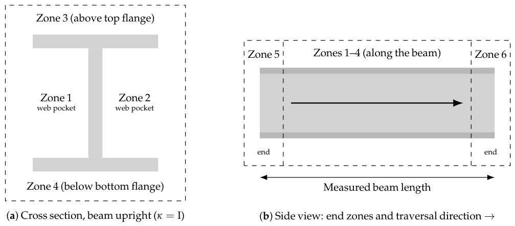
The beam’s bounding box induces six zones (Figure 5): zones 1 and 2 are the two web pockets, the regions between the flanges on either side of the web; zone 3 lies above the top flange and zone 4 below the bottom flange; zones 5 and 6 are the two beam ends. Zones are traversed in numerical order, 1 to 6. Parts are assigned to zones by a vertex vote: each vertex of the part’s CAD mesh votes for the zone that contains it, and the part goes to the zone with the most votes. Within the fixed zone traversal, three pairwise rules order the parts: overlapping parts are placed centre-outward; touching parts are placed support-first, i.e., a part on which another part rests is placed before it; and parts closer than 20 mm are ordered bottom-up. Within a zone-priority group, parts are sorted along the beam: in the web pockets from the far end toward the near end (zone 1) and the reverse (zone 2), above the top flange bottom-up and then along the beam. For example, a bracket that rests on a stiffener is placed after the stiffener, and of two stiffeners 15 mm apart, the lower one is placed first. Sequencing thus costs a sort, not a search; the price—no global optimality—is examined in the discussion.
Figure 4.
Planning process with decision layers. Setup layer: enumeration, one parallel feasibility simulation per candidate setup, selection. Part layer of the offline sweep (dashed box, executed inside every container): ordering, then for each part a grasp from which a path to the placement pose can be planned, a traversable approach corridor, and at least one weldable seam; a part that fails on every graspable face is recorded as missed and the simulation continues with the next part. Program layer: the online planner re-plans each part of the selected plan completely (pick, transfer, full placement chain, up to three seams), the program is emitted as RAPID, and the cell executes it with the operator in the loop.
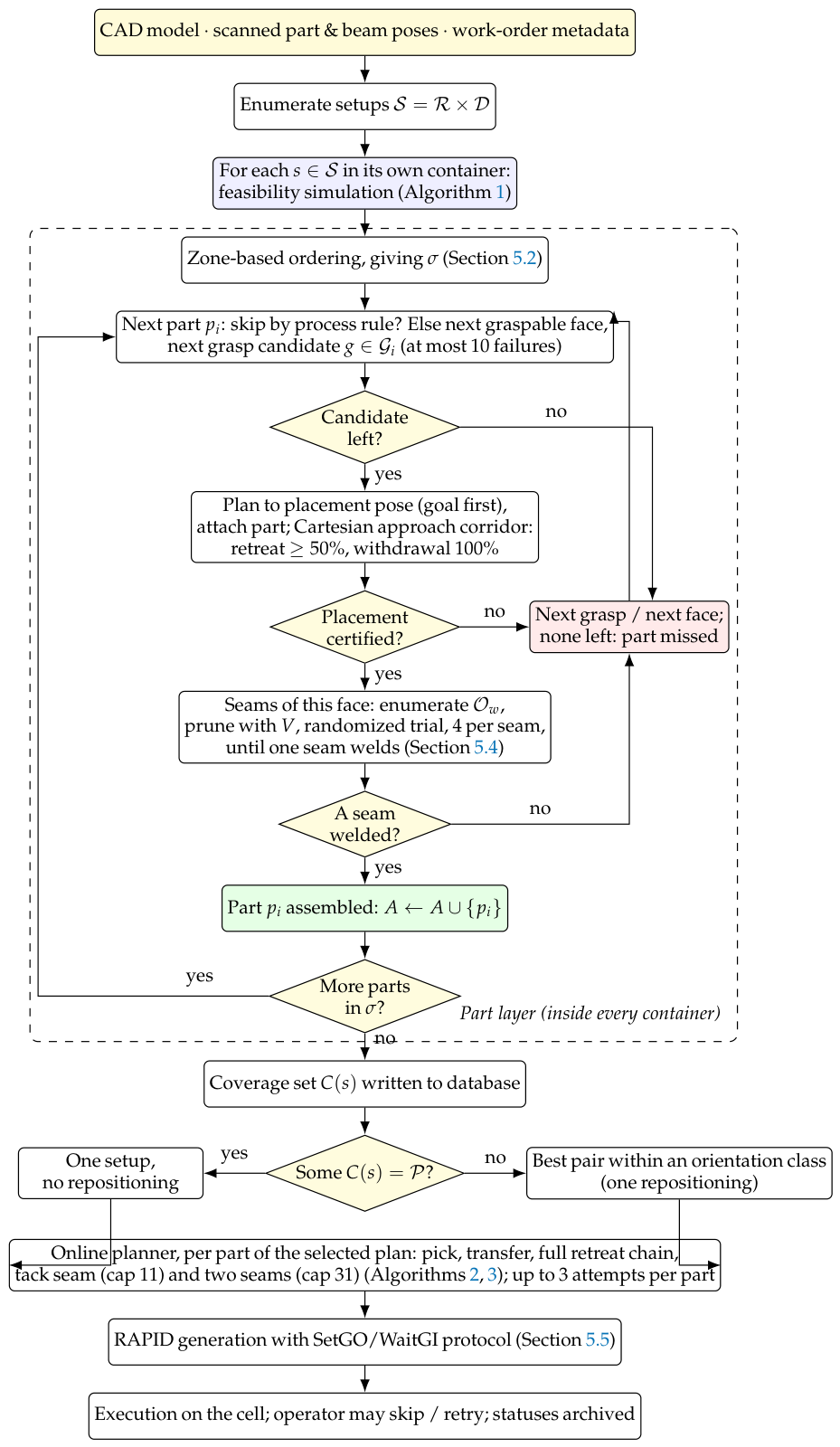
Figure 5.
The six zones induced by the beam’s bounding box. (a) In the cross section: the two web pockets between the flanges (zones 1–2), the region above the top flange (3) and below the bottom flange (4). (b) Along the beam: the two end regions (5–6). A part is assigned to the zone that contains most of its mesh vertices; zones are traversed in a fixed order and parts within a zone are sorted along the beam axis after the pairwise priority rules are applied. Rotating the beam to the on-side class () turns a web pocket upward, which is what makes parts unreachable in one class reachable in the other.
5.3. Placement: Grasp Search and Reverse Retreat Planning
For each part, the online planner filters grasp candidates by cheap tests before any motion planning. Grasp candidates are precomputed per part from its CAD mesh. Every planar face that will not be in contact with the beam is a candidate face. On it, a grid of magnet positions is crossed with rotations of the gripper about the face normal. Each resulting gripper pose passes three geometric checks before it is stored: the magnet footprint must lie within the face; it must not intersect the bounds reserved for the part’s contact faces, its zone, or the beam supports; and the overlap area between magnet and face, scaled by the magnet’s holding coefficient, must exceed the part’s weight by a safety factor (1.5 for the large magnet, 3 for the small one). Candidates are then interleaved across faces so that consecutive attempts try different faces. At planning time three further cheap tests discard candidates without a planner call: (1) The face resting on the table is excluded, since it cannot be reached. (2) Candidates whose gripper axis lies within of the horizontal are rejected, because a magnet acting sideways cannot hold the part securely during transfer. (3) A two-pose inverse-kinematics probe checks that the gripper pose over the part on the table and the same gripper pose transformed to the part’s target on the beam both admit an IK solution within joint limits; a candidate that fails either is discarded. Failed gripper poses are cached so that a face rejected for one part instance is not re-tested when the part is attempted again. Surviving candidates enter a four-stage chain (Algorithm 2). (i) Reverse retreat planning: From the placement pose on the beam, a chain of retreating waypoints along the press vector (, , the vector plus a vertical clearance) is planned goal-backwards and replayed forwards. The most constrained pose (the part in contact with the beam, between already installed neighbours) is thus tested first, and a failure costs one query instead of a whole chain. (ii) Pick to neutral: The track (external axis) moves the assembler alongside the part on the table, the arm plans a path to a pre-pick pose above the part, descends onto it, the magnet is switched on, the part is attached to the gripper as a collision object in the planning scene (so that subsequent planning treats robot and part as one body), and the arm lifts. (iii) Neutral to place: Joint reconfiguration to a safe intermediate posture, then the linear approach through the retreat chain in reverse, a PLC handshake that hands the welder its turn, magnet release. (iv) Welding, described below: A part gets up to three full attempts; the RAPID instructions emitted during a failed attempt are discarded and generation resumes from the program preamble (the section buffering of Section 5.5).
| Algorithm 2 PlacePart (online planner): grasp filtering and reverse retreat planning for one part. |
Require: part with table pose , target , press vector , grasp candidates (gripper poses in the part frame), scene
|
5.4. Welding: Torch Discretization, Geometric Pre-Validation, Randomized Trial
Each seam carries a torch vector from CAD. A local frame is built (torch vector as Z, world-up projection as X), and candidate orientations are enumerated as in Equation (2): rotations about the torch axis in steps crossed with 25 graded work-angle tilts of up to per axis—600 candidates per seam. Figure 3 shows the geometry. The tool centre point (TCP) of the torch is the wire tip; the seam frame places the TCP on the seam line with the torch axis along the CAD torch vector . Rotating the torch about by changes where the torch body and the robot wrist sit around the seam without changing the wire’s contact point: this is the functional redundancy of welding that Section 2.3 discussed. Tilting by toward one flank of the joint changes the work angle within the process tolerance. Both are enumerated because either may be what turns an unreachable seam into a reachable one: rotating about moves the wrist away from a neighbouring part, tilting moves the nozzle out of a pocket. The validator V of Section 4 prunes them before any planning. Skip rules are applied first: seams shorter than 30 mm, overhead seams, and seams whose partner part is not yet placed are not attempted. The surviving orientations are then tried in random order, at most of them, and the first one for which the approach, the seam start, the linear seam traversal, and the retreat can all be planned as Cartesian paths is taken (Algorithm 3); no ranking is attempted. Welds are executed as tack pairs (two sub-seams with a central gap) or full passes; a seam whose end proves unreachable is recorded and executed as a half seam (Figure 6).
| Algorithm 3 WeldSeam: torch orientation search for one seam ( in the sweep, where WeldAnySeam calls it until one seam of the part succeeds; for the online tack seam and 31 in the online welding pass, which welds two seams per part). |
Require: seam w (start, mid, end, torch vector ), scene , attempt cap
|
Figure 6.
Tack welds on a production assembly, as emitted by the planner: each part is fixed by short paired tacks before full seams are laid, so a downstream failure never leaves a part half-welded along its full length.
During welds, the assembler’s planning-scene geometry is inflated (its collision bodies are enlarged by a safety margin) so the welder plans against a conservative model of its idle partner.
5.5. RAPID Generation and Execution
Plans are compiled to native RAPID, one module per robot. A module contains joint and linear moves with the track position as an external axis, arc start and end instructions, magnet and wire-service (torch cleaning and wire cutting) commands, and the inter-robot protocol itself: the group-output/group-input handshakes (SetGO/WaitGI) between the two controllers and the PLC are emitted as part of the program. Synchronization is therefore a property of the generated code, not of a run-time coordinator. Generation is section-buffered: the instructions of a module are accumulated in two text buffers, a preparation section (procedure header and motion settings, gripper selection, the opening handshake, a flip at the flipper station if the part is flagged, torch cleaning) and a work section (the moves and process commands of the current attempt); a failed attempt clears only the work section, and the two sections are concatenated on success. Delivery is deliberately simple: module files are written to a directory shared with the robot controllers, and a one-line message over a TCP socket to the controller starts the program; execution state (assembled, failed, skipped parts) is kept in the database, so that an executor restarted after an interruption resumes from the recorded state without repeating completed operations (idempotent under restart).
6. Experiments
6.1. Setup Coverage on Production Work Orders (Hypothesis 1)
The production database archived the per-setup feasibility simulations themselves, allowing Hypothesis 1 to be evaluated on real work orders without re-running the stack. Two corpora were available. The cell was deployed at two production sites; we call them site A (the first deployment, 2023–2024) and site B (the second, 2025–2026). At site B the archive holds the complete candidate sweep—every setup tried and its coverage set—for six assemblies, each simulated under 12–19 candidate beam setups (only setups whose simulation ran to completion were counted; a seventh assembly whose sweep never completed was excluded). These six admit the full comparison of selection rules in Table 2. At site A the archive holds, for every assembly planned, the setups the production rule selected and their coverage sets, but not the rejected candidates; this corpus is far larger (250 distinct assembly designs after merging series-produced repeats of one design) and supports the first half of Hypothesis 1 stratified by work-order size (Table 3), but not the comparison with the exhaustive optimum.
Table 3.
Setup coverage at site A (the first deployment): production plans for 250 distinct assembly designs, stratified by work-order size. Single suffices: one setup covered every part; plan suffices: the selected plan (one or two setups) covered every part; best single: median fraction of parts covered by the better setup of the plan.
Figure 7 visualizes the same data. The archived run times also give the cost of the search: a feasibility simulation of a whole work order costs a median of 9.7 min per setup (90th percentile: 22.4), and the enumeration is fully parallel across containers; the entire setup sweep completes in roughly the time of its slowest member.
Figure 7.
Setup coverage on six production work orders (archived feasibility simulations). Grey: work-order size; light blue: best single setup; orange: the deployed pair, restricted to one orientation class; blue: unrestricted greedy pair; dark blue: exhaustive best pair; darkest: union over all tried setups. The gap between the darkest bar and grey is the cell’s coverage ceiling, parts no setup can reach.
Three findings. First, a single setup is almost never enough: only the smallest assembly (five parts) is fully covered by one setup; on the others, the best single setup covers 50–73% of the coverable parts (those in the union over all tried setups).
Second, greedy pairing is near-optimal: the greedy pair (best single setup plus best complement) equals the exhaustive best pair on five of six assemblies and lost two parts on the sixth. The deployed rule, which restricts the pair to one orientation class, is not near-optimal: it matches the unrestricted greedy pair on three assemblies and loses two parts on each of the other three (1R1, 3SA21, SK2), six parts of the 89 in the corpus, or 10% of the parts the unrestricted rule would cover. The restriction buys a cheaper repositioning (a rotation or an axial shift on the existing supports, with the part-face flags and the beam scan remaining valid), and the archive now gives the cost of that convenience. Note that these are statements about coverage, not about cost: all three rules consume the same precomputed per-setup coverage sets, over which even exhaustive pairing is a handful of set unions. The expense is the simulation that produces those sets, and every rule pays it in full.
Third, and unplanned: coverage has a ceiling below the work order—on four assemblies even the union of all tried setups leaves parts unassemblable (most severely 14 of 30 parts coverable; 23 of the 89 parts in total), meaning some parts fail in every beam position and require manual placement. The feasibility archive thus doubles as a design diagnostic, with one qualification that Section 6.3 makes necessary: the archived simulations all ran at the production per-query budget, and the budget sweep shows coverage to be strongly budget-limited at that operating point. Parts that no tried setup covers are therefore parts the cell as configured cannot handle; some fraction may be reachable with a larger planning budget rather than different fixturing, and the archive cannot split the two. Hypothesis 1 is supported on field data under that reading, on both corpora for its first clause and on the fully swept corpus for its second.
Second corpus: 250 assembly designs from site A. Table 3 tests the first half of Hypothesis 1 at scale. Each record is the plan the production rule selected for one assembly: one setup if it covered the whole work order, otherwise the pair (five records list a single setup that does not cover the order, because the second setup was not archived; they count as not completed). Series-produced assemblies share one CAD design, so their records are not independent samples. We identify a design by its part marks, weight, and weld set in the design archive and keep the latest record per design, which reduces 308 records to 250 distinct designs of 2–37 parts (median 10); records of the same design never differed in outcome. Across the corpus a single setup covered the whole work order for 43 of 250 designs (17%), the selected plan covered it for 211 (84%), and the better setup of the selected plan covered a median of 56% of the parts. That last figure is a lower bound on the best single setup, since rejected candidates were not archived at that site; it is of the same order as the 50–73% measured on the fully swept corpus at site B, but the two are not defined identically and we do not treat them as one measurement. The pattern holds in every stratum: no stratum has more than 30% of designs coverable by one setup, and the two-setup plan completes 60–87% of them. The corpus cannot say how far the selected pair lies from the exhaustive optimum, because the rejected candidates were not archived at that site, but it establishes on a second installation of the cell, a different product mix, and a sample forty times larger that the premise of the design—one setup is rarely enough, two usually are—is not an artefact of six work orders. Site A completes far more work orders than site B (84% against two of six), which we attribute to smaller work orders and simpler structures rather than to the planner; the corpora are not compared beyond this. One caveat: these records were produced by an earlier revision of the same system, and we have not verified that every parameter (planner, per-query budget) matched the later deployment, which is a further reason to consider this corpus for the first clause of Hypothesis 1 only.
6.2. What the Cell Actually Did with the Plans
Every experiment above measured the planning system against its own simulation. The task archive of site B also recorded what happened when the generated programs ran: the executor wrote a per-part, per-operation status back to the task record, the operator’s console actions were logged with timestamps, and each stage of the pipeline was stamped with start and end times. Throughout this section a task is one execution attempt of an assembly’s work order; several tasks can belong to one assembly. The 264 tasks with such records (221 cancelled, 41 archived, two tests) belonged to 16 assemblies; 84 of them, on seven assemblies, reached execution on the cell. Tasks were not independent samples: one assembly alone accounted for 115 records, so we report per-assembly figures alongside per-task ones. This is the only evidence in this paper that does not pass through the simulator, so we state plainly what it can and cannot support: it is not a controlled experiment, the sample is dominated by cancelled tasks, and no independent observer verified the executor’s own status reports.
Committed motions succeed on the floor, with three recorded qualifications. Of the operations that reached a terminal state (Table 4), 170 of 183 part installations (92.9%) and 188 of 195 welds (96.4%) were recorded as successful; per task, the median operation success rate was 100%, and 81% of executing tasks completed every attempted operation. These are final statuses: the log recorded 478 operator retry actions across the corpus, and the archive does not distinguish first-attempt from post-retry success, so the rates describe what the cell ultimately achieved with an operator in the loop, not unattended execution. Operations cancelled mid-flight remained in queued or running states (13 installations and 26 welds) and were excluded from the denominator, which censored some failures. And the statuses were the executor’s own reports: a completed weld program, not an inspected weld. Within those limits the conclusion stands: the plans the system certifies are executable on the floor with high probability with an operator in the loop.
Table 4.
Production execution records from the task archive (264 tasks with execution or operator-log entries; 84 reached execution). Operation counts exclude records captured mid-flight in a queued or running state.
What limits throughput is coverage, not motion quality. The same records showed a median of 10 parts per task marked to be skipped, with at least one skipped part in 83% of tasks and up to 24 in the worst case. The per-task figures were dominated by the assembly with 115 records (median 20 parts skipped); per assembly, taking each assembly’s last recorded task, the median was 2 parts skipped (maximum 22) and 11 of 16 assemblies had at least one. Operators issued 478 retry actions in total, and 40% of tasks required at least one. The console log held 17 archiving verdicts on six assemblies; three of the six were eventually archived as successfully completed. The picture is consistent across every independent line of evidence in this paper: the per-motion reliability is high, and the assembly nonetheless does not finish, because a substantial fraction of the work order is never attempted. That is precisely the coverage ceiling measured in Section 6.1 from the simulation side—four of six assemblies had parts that no tried setup could reach—and it is the strongest support the archive offers for Hypothesis 1. It also sharpens the diagnostic reading of Section 6.1: the parts skipped on the floor correspond to the parts the simulation could not cover, though we cannot separate parts skipped because no setup reached them from parts skipped at the operator’s discretion, since the record does not distinguish the two.
Cycle time. The stage timestamps give the production cost of each pipeline element (median over tasks): part scanning 1.8 min, part matching 0.5 min, beam scanning 2.7 min, beam matching 0.6 min, part and beam inspection 0.1 and 0.3 min, planning 2.9 min, and execution 11.2 min (a median over a corpus dominated by cancelled runs, so it understates full assemblies). Two planning figures coexist and must not be conflated: the logged 2.9 min is the online planning stage of an execution cycle, whereas the offline feasibility sweep of Section 6.1 costs a median 9.7 min per candidate setup and runs before the task starts. Online, perception plus planning together cost under 9 minutes against 11 minutes of robot motion, the quantitative justification for spending planning time on verification rather than optimization.
6.3. Planner Portfolio Under a Tight Budget (Hypothesis 3)
The archived simulations all ran the production default, so testing Hypothesis 3 required rebuilding the planning software. We rebuilt the cell’s ROS/MoveIt container and replaced its dependency on the remote task API, since decommissioned, with a local service backed by the restored production database. We then ran the feasibility simulation once with each of the sixteen planners of the portfolio on one fixed problem: the 24-part assembly SK2 of Table 2 in a single beam setup (rotation , axial shift mm). All other parameters—the 0.1 s per-query budget, the goal tolerances, the 50-attempt cap—were left at production values. The score is the number of parts the feasibility simulation manages to place. Table 5 expands the planner names used in the sweep.
Table 5.
OMPL planners in the cell’s portfolio (as named in Table 6), with the mechanism each uses. The asterisk is part of the planner name and marks the asymptotically optimal variant [16]; the same convention applies in the tables and figures that follow.
The budget partitioned the portfolio into three regimes (Table 6), and the most consequential boundary was not where we expected it.
Table 6.
Planner census on a fixed 24-part assembly (SK2) in a single beam setup, all other parameters at production values (0.1 s per-query budget). Single runs at the production budget; the repeated budget sweep of Figure 8 supersedes any per-planner reading of this census. Preparation-stage failures were each reproduced in isolation.
Six entries never reach the assembly at all. They abort in under five seconds, raising the pipeline’s joint-motion exception on the preparation stage, the fixed pair of joint-space moves that sends each robot to its home posture before any part is considered. Five fail on the very first of these, a move of the assembler to its all-zero configuration; TRRT survives that one and fails on the next. The goal is not the difficulty: all-zeros lies comfortably inside every joint limit in the cell model, and eight other planners solve the same move under the same conditions. Nor is it the harness: we re-ran each failing entry in isolation, with no concurrent load, and every one reproduced its failure identically. Under a 0.1 s budget these planners simply cannot return a path to a trivial joint-space goal, and because the pipeline treats a failed preparation move as fatal, the entire work order is lost before planning begins. A portfolio evaluated only on the assemblies it completes would never see this failure mode.
Seven entries complete the sweep at the production budget. Because a single run of a randomized planner is not a measurement, we then repeated the four representative planners (PRM*, PRM, RRTConnect, RRT) three times each at three per-query budgets—the production 0.1 s, 0.25 s, and 0.5 s—for 36 runs in total (Figure 8). The repetition immediately disciplined the single-run census: run-to-run spread within one planner reached five parts, larger than any single-budget gap between planners, so per-planner rankings at a fixed budget are not significant, and we do not report them as such. What survives repetition are three structural facts.
First, the failure regime is a budget threshold, and it is stochastic near the boundary. At 0.1 s the roadmap planners never abort (6/6 runs), RRTConnect aborts in one run of three, and RRT in all three; at 0.25 s RRTConnect always survives; at 0.5 s even RRT clears the preparation stage in one run of three. What looked like a fixed partition in the single runs is a per-planner budget threshold. Because the threshold moves with the budget, the same structure should appear on native hardware at lower budgets.
Second, the ordering among survivors is budget-dependent and, at any single budget, inside the noise. At the production 0.1 s the roadmap planners never abort and place more parts (medians four against two), while RRTConnect sits at its survival boundary; at 0.25 s RRTConnect’s runs (10–12) overlap the roadmaps’ (6–11), so no per-planner ranking clears the five-part run-to-run spread, and we make none. What is established is weaker and more useful: the planner that was marginal at one budget is fully competitive one step up, so any single-budget comparison—including our own census above—is an artefact of its operating point, and the transferable object is the coverage-versus-budget curve, not a ranking. On Hypothesis 3 the verdict is: supported—planner and budget interact strongly and the production point is budget-sensitive—while a fixed family ordering at one budget is refuted by the shift.
Third, coverage roughly doubles from 0.1 s to 0.25 s and shows no further gain at 0.5 s (whether it is truly saturated or still rising past 0.5 s is untested): the production planner’s own medians rise from five to 10 parts of 24 at +0.15 s per query, in a pipeline whose planning stage occupies about three minutes of a twenty-minute cycle (Section 6.2). The per-query budget, not the planner, is the sweep’s binding hyperparameter. One caveat prevents converting this into a direct production prescription: the budgets are emulated wall clock. If the emulation slowdown is the order of magnitude we conservatively assumed, the native 0.1 s budget already lies past the saturation knee, and nothing should change. If it is closer to the 3–4× suggested by a rough cross-check against archived native simulation times, the production budget is materially starved, and doubling it would roughly double coverage. The calibration in the threats-to-validity paragraph below favours the second case. One calibrated run on the cell hardware would distinguish the two cases; it is the first measurement to make.
Two secondary observations matter more for engineering than for the ranking. First, wall clock is essentially flat across planners—1839 s to 2190 s in the single-run census—and across budgets—1938 s to 2449 s over the 26 repeated runs that completed and placed parts (nine aborted at the preparation stage; one RRT run at 0.5 s cleared it, placed nothing, and ended after 793 s)— and uncorrelated with how many parts were placed. The cost of one feasibility simulation is dominated by its fixed enumeration of candidate placements, not by planning success, so a better planner buys coverage at no time penalty; this is what makes portfolio selection worth doing at all. Second, even at the most generous budget swept, no planner exceeds 12 of 24 parts in a single setup. That is not a planner failure but the central fact the pipeline is built around: no single beam setup reaches most of an assembly, which is precisely the argument for the multi-setup coverage machinery of Section 6.1.
The planner census also surfaced a live configuration defect. One selector entry requested the planner “BKPI”, a truncation of BKPIECE that matched no planner registered in the cell’s OMPL configuration. It is the one failing entry that did not raise the joint-motion exception, failing earlier and differently. Because an unrecognized planner identifier did not surface as an error to the operator, that portfolio slot had been silently unusable. Validating a planner portfolio against the registered configuration at startup is a one-line check that this deployment lacked.
Threats to validity. The stack ran under CPU emulation (the x86-64 production image executed through Docker’s QEMU layer on an Apple-silicon host: Docker Desktop 4.20.1 with Docker Engine 24.0.2 (Docker, Inc., Palo Alto, CA, USA) on a MacBook Pro with an Apple M1 Pro chip and 16 GB of memory (Apple Inc., Cupertino, CA, USA)) at roughly an order of magnitude below native speed, and the budgets were wall clock, so the absolute numbers understate the deployed system and the thresholds reported here map to lower native budgets. One archived native run calibrates the slowdown: the production sweep of the same assembly in the stand- setup nearest to the one used here (axial shift mm against mm) placed 11 parts at the native 0.1 s budget, between the emulated medians at 0.1 s (5) and at 0.25–0.5 s (10), which points to a factor of roughly three to five rather than an order of magnitude. The budget sweep partially answers this concern: the regime boundary moves with budget exactly as a harness-independent mechanism predicts, so the structure (thresholds, inversion, saturation) transfers even though the specific budget values do not. Confirming the native operating point is the first measurement to run with cell access. One entry (SPARS) ran for 2 h 22 min before the emulation layer itself raised a segmentation fault; that failure is an artefact of the emulation rather than a property of the planner, and we excluded it. Finally, this is one assembly in one setup: the regime structure and the family-level ordering are the transferable conclusions, and a portfolio recommendation for a different cell would need its own sweep.
6.4. Torch Pre-Validation on Real Weld Geometry (Hypothesis 2)
The geometric validator is pure geometry, so its pruning behaviour is measurable without the motion-planning stack: we imported the unmodified production seam and validator modules and ran them over 1580 welds from 15 production assemblies in the CAD archive (Figure 9). Of the 600 discretized torch orientations per seam, a median of 72 survived the validator (the always-retained nominal orientation included), a pruning factor of 8.3× with a tight spread (10th–90th percentile: 67–77 survivors). No seam was pruned to zero, so the geometric stage never declared a seam infeasible on its own. Whether the orientations it discarded were reachable is a different question, and one this experiment cannot answer: establishing a false-rejection rate requires planning the pruned orientations against the live stack, which we flag as the main gap in this evaluation. Since the surviving set feeds a randomized search under a fixed attempt cap, the pruning is what makes that cap a meaningful sample: in the offline sweep, four trials drawn from the full 600-candidate discretization covered 0.7% of it, whereas four drawn from the 72 survivors covered 5.6%; in the online planner, whose cap was 31, the same figures were 5% and 43%. Section 6.5 measures what happens to coverage when the validator is switched off with the sweep’s cap in place.
Figure 8.
Repeated planner runs across per-query budgets (3 repetitions per cell). (a) Coverage per run versus budget, lines joining the medians per planner: coverage doubles from 0.1 s to 0.25 s and shows no further gain at 0.5 s; once RRTConnect clears its survival threshold its runs overlap those of the roadmap planners, so no single-budget ranking survives the run-to-run spread. (b) Share of runs aborting at the preparation stage: the failure regime dissolves gradually with budget, planner by planner.
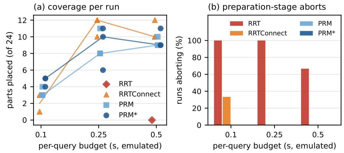
Figure 9.
Production torch pre-validation measured on 1580 real welds from 15 assemblies (unmodified production code). (a) Orientations passing the validator per seam, out of 600 candidates: median 72 (solid line; dashed lines mark the 10th and 90th percentiles), never zero. (b) Seam-mode census in the beam’s CAD pose: 37.9% of welds are overhead and unweldable without repositioning the beam.
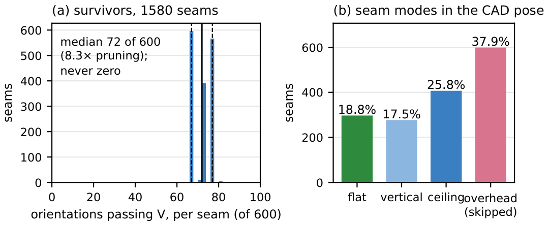
The same sweep yielded a census with direct consequences for setup selection: in the beam’s CAD pose, under the validator’s own mode test (torch-vector inclination against gravity), only 18.8% of welds were flat, 17.5% vertical, and 25.8% ceiling (below the beam axis, torch not pointing upward), while 37.9% were overhead (torch pointing upward, ), the orientation class the production rules skip outright. More than a third of CAD-specified welds were thus unweldable as posed, and beam repositioning (Section 6.1) is not an optimization but the mechanism that converts overhead seams into weldable ones. Hypothesis 2 is supported in its measurable half, the pruning factor and its safety; the false-rejection rate against motion-planning ground truth still requires the live stack.
Why a CAD-specified weld can be infeasible. A reader may reasonably ask how a seam defined on the CAD model can fail to be weldable when the beam can be rotated to four orientations and the welding robot rides a 14.6 m track. Three mechanisms account for it; Figure 10 illustrates the first two on the cross-section of a production beam, and Figure 11 shows the simulation scene in which all three are decided. (1) Process rule, not reach. In the beam’s delivered pose, 37.9% of seams are overhead (torch pointing up into the joint); they are excluded by the welding process rule, not by the planner, and only a rotation of the beam brings them into a permitted mode, which is exactly why setup selection exists. On the 24-part assembly used throughout Section 6.3, 109 of its 233 seam segments (47%) point upward in the delivered pose: every fillet on the underside of the top flange and on the upper face of every horizontal plate. Rotating the beam by turns these into flat seams and turns the bottom-flange fillets overhead. Two qualifications follow from the algorithms. A part is certified as soon as one of its seams is weldable, so an overhead seam removes a part from only when every seam of the part is overhead in that setup (plates on the underside of a flange are the typical case); otherwise, it removes the seam, not the part. And the generated programs weld each part only under the setup to which it is assigned, with up to three seams per part (Section 4); seams that are overhead there are not welded by the cell. Repositioning therefore makes such seams weldable; welding them is outside the current programs. (2) Collision inside the joint. Most seams are fillet welds between a stiffener and a flange, inside a web pocket that may be only a few hundred millimetres wide; the torch, its nozzle, and the robot’s wrist must fit between the stiffener, the neighbouring stiffener, and both flanges while holding the work angle within tolerance. The reach of the arm is irrelevant if the wrist collides with the adjacent part, and the parts already installed change this geometry seam by seam. (3) Inverse kinematics along the whole seam. A seam is executed as a linear Cartesian traversal at a fixed torch orientation; every point of the traversal must have a collision-free IK solution within joint limits at that orientation, and the track adds one redundant degree of freedom but cannot move during the traversal. A seam whose start is reachable and whose end is not is downgraded to a half seam (Section 5.4). The torch census above measures (1) exactly; (2) and (3) are what the motion-planning stage of Algorithm 3 decides, and the execution records of Section 6.2 show that the seam programs to which the cell commits succeed in 96.4% of terminal-state records, with the qualifications stated there.
6.5. Ablations and Baselines
Two questions remain: what each component of the system contributes, and how the system compares with alternatives. There was no external planner that solves this cell’s problem end to end against which a like-for-like comparison could be run, so the baselines were internal: for each component, we compared the deployed choice with the natural alternative—the component removed, or replaced by the simplest rule—on the same production data or on the same simulated work order. Table 7 collects the results; the sources are the archive analyses above and a set of controlled runs on the rebuilt stack, executed with the same harness as the budget sweep (SK2, one beam setup, PRM*, three repetitions per condition, per-query budget 0.25 s, all other parameters at production values). The baseline condition is a new set of three runs made alongside the ablated ones, not the three PRM* runs at 0.25 s of Section 6.3 (six, 11, 10); the six together (median 8.5) show the run-to-run spread against which the ablations should be judged.
Table 7.
Component ablations. Archive rows use production data (Section 6.1 and Section 6.4); stack rows are controlled runs on the rebuilt production stack (SK2, 24 parts, one setup, PRM*, 0.25 s per query, three repetitions; parts placed are given per run).
Setup selection. The archive prices every alternative to the deployed rule on the six fully swept work orders. Without repositioning the cell would install 42 of 89 parts; the deployed within-class pair installs 54; lifting the class restriction (greedy) installs 60 and the exhaustive pair 62; even the union over every setup tried reaches only 66, because 23 parts are unreachable under any setup at the production budget. Two conclusions follow. The repositioning machinery is worth parts (a 29% gain over the best single setup), and the class restriction costs six of those. Greedy selection loses two parts to exhaustive search on one assembly and nothing elsewhere, so the worst-case guarantee of Section 4 is loose in practice. On the 250-design corpus, the same comparison yields one setup completing 17% of work orders and the production plan 84%.
Figure 10.
Why a CAD-defined seam can be infeasible, on the cross-section of the 24-part production beam of Section 6.3 (I-profile 390 × 300 mm, web pockets about 140 mm deep). Colours: grey, beam flanges and web; light blue, stiffeners; green, the fillet weld under consideration; red, the fillet that would be overhead, with the torch orientation it would require drawn dashed in red; the torch at its working orientation is drawn in light blue. (a) With the beam upright, the fillet between a stiffener and the bottom flange is welded with the torch pointing downward (flat, permitted), but the fillet between the same stiffener and the underside of the top flange would require the torch to point upward: it is overhead and skipped by process rule. On this assembly, 109 of 233 seam segments (47%) are overhead in the delivered pose. (b) Rotating the beam by exchanges the two cases; this is the repositioning that setup selection computes. (c) Inside a pocket, the torch approaches a fillet at ; the 28 mm nozzle and the wrist behind it must clear the neighbouring stiffener at spacing a and the flange tip, and the seam must be traversable at that orientation along its whole length. Reach along the 14.6 m track is not what limits these seams.
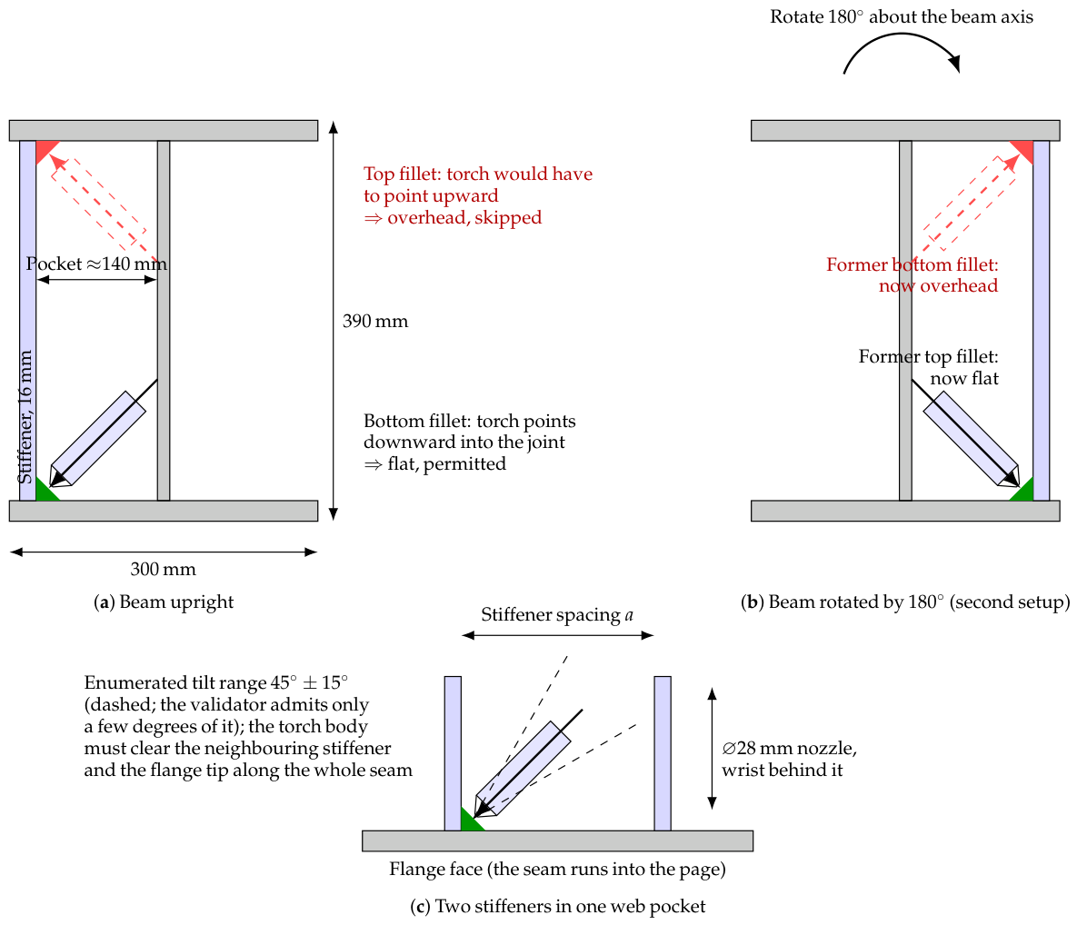
Torch pre-validation. On the archive, the validator’s effect was a change in sampling density: with the sweep’s cap of four trials, the search sampled 5.6% of the admissible orientations when the validator was on and 0.7% of all orientations when it was off. On the stack, the effect was large: with the validator switched off and everything else unchanged, the three runs placed five, three, and three parts against eight, eight, and nine with it on, and the number of seams that exhausted their four trials rose from 18–20 per run to 38–45. The runs were also a third shorter (22–24 min against 33–35), because parts failed earlier. At the sweep’s attempt cap the validator is therefore the difference between a search that usually finds a weldable orientation and one that usually does not. Since four draws from 600 candidates sample a far sparser set than four from 72, the ablation is equivalent to an eightfold change in the attempt cap; it does not separate the validator’s selectivity from that sampling-density effect. Whether it also rejects orientations that would have planned (its false-rejection rate) remains unmeasured, as stated in Section 6.4; the ablation bounds the net effect, which is strongly positive.
Figure 11.
The simulation scene in which every feasibility check of this paper was run: the MoveIt planning scene of the cell, rendered in RViz from the cell’s own URDF model during the check of one part. The assembler (far track, on its carriage) holds the part (purple) at its target near the end of the beam (blue), which rests on its two supports between the tracks with the parts installed so far (grey); the welder (front track, on its column) has brought the torch to a seam of that part; the preparation table lies behind the beam. The two arms are the kinematic models of the cell’s ABB IRB 6700 (material handling) and ABB IRB 2600-series (welding) manipulators, each on its linear track; robot links are drawn in light grey, and no colour in the scene carries meaning. Robots, tracks, carriages, supports, beam, table, and every installed part are collision bodies; a weld is feasible only if the torch, nozzle, and wrist fit into the joint at an admissible orientation along the whole seam.
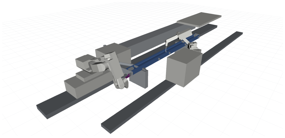
Zone-based ordering. Removing the pairwise priority rules and the within-zone sort (zone traversal kept, parts inside a zone in CAD order) placed five, nine, and eight parts against eight, eight, and nine with the rules on. The difference is inside the run-to-run spread of the planner, so on this work order the ordering rules do not measurably change coverage. We report this as a negative result. The rules exist to avoid placements that a neighbouring part would physically block (support-first, centre-outward), and this work order—stiffeners along a single beam with few stacked contacts—may simply not exercise them; a coverage benefit on such orders is not something the data support, and we do not claim one. Their cost is nil (a sort), which is why they remain. The zone partition itself was kept in the ablation because the enumeration of axial shifts (Section 5.1) and the end-zone rules of Algorithm 3 depend on it; removing it would change the candidate setups, not only the order.
Reverse retreat planning. Planning the placement chain goal-first does not change which parts are feasible, up to the randomness of the planner—the same poses must all be reachable in either order—so its contribution is a matter of planning work rather than coverage. What follows is a counterfactual count from the failure stages recorded in the baseline runs, not an ablation run. The sweep applies the same goal-first logic in miniature (placement pose first, then the approach corridor), so the baseline runs record at which step each placement attempt failed. Across the three baseline runs the sweep made 200 placement attempts that failed: 175 of them (88%) failed at the placement pose itself, the first query in the goal-first order, 14 at the retreat corridor, and 11 at the post-placement withdrawal. Under a forward order, the same 175 attempts would each have planned the approach corridor before discovering that the goal is unreachable, spending two further queries on each of them without changing which parts are certified. The same argument applies with more force to the online planner’s four-stage chain (Algorithm 2), where a forward order would plan three waypoint segments before reaching the goal.
What was not compared. We did not compare against an optimization-based assembly sequence planner or a task-and-motion planner, because none of the published methods of Section 2 takes this cell’s inputs (scanned part poses, a measured beam, two track-mounted robots with a PLC protocol) and produces executable programs; porting one would mean re-implementing most of this system around it, and the comparison would then measure the port. The internal baselines above are the comparisons the production data can support.
7. Discussion
Feasibility as the product. The system never asks, “What is the best plan?”; it asks, “Does a plan exist, and under which setup?”, and buys certainty by parallel verification. This inversion fits fabrication economics: a beam repositioning costs minutes, a failed weld on the shop floor costs an order of magnitude more, and compute is the cheapest resource in the loop. The same inversion appears at every scale: grasp candidates are verified, not ranked; torch orientations are pruned then tried, not optimized; the retreat chain is planned backwards from the only pose that matters.
Synchronization compiled into the artefact. Emitting the PLC handshakes inside the generated RAPID makes the two-robot protocol inspectable and replayable, the coordination exists in a text file, not in a live process. The cost is expressiveness: the alternating-phase protocol cannot overlap the robots’ work, and the throughput ceiling this imposes is untouched by any planning improvement.
What transfers, and what does not. Two questions concern transferability: how the approach adapts to more complex scenarios, and whether its evidence is tied to one production line. Two parts of the design are cell-independent. The first is the inversion itself: wherever a fabrication task couples a small discrete choice (workpiece setup, fixture, station) with motion feasibility that is expensive to derive but cheap to check, the feasibility sweep and the coverage-maximization rule of Section 4 apply unchanged, and the greedy guarantee holds for any monotone coverage function. The second is the use of the feasibility archive as a diagnostic: the parts that no setup covers are a statement about the cell, not about the planner, and any deployment that stores its sweeps obtains that diagnostic for free. Three parts are specific to this cell and would have to be re-derived for another. The zone partition assumes an I- or H-section main member; a truss, a box column, or a member with three-dimensional bracing needs its own partition or a learned one. The grasp model assumes magnetic pick-up of ferrous plates on planar faces; mechanical grippers or non-planar parts change the candidate generator, not the search. The alternate-phase protocol assumes two robots whose workspaces overlap only at the beam; a cell in which several welders work concurrently needs the coordination the surveys of Section 2.5 address, which this system deliberately avoids. The evidence base is now two production deployments of the same cell type (Section 6.1): the second corpus shows that the premise of the design holds across a different product mix and a different site, but it does not show that the specific rules transfer to a different cell type, and we make no such claim.
Limitations of the method. Kinematic simulation certifies geometry, not dynamics: velocity and acceleration limits are unmodelled, and the deliberately tight 0.1 s per-query budget with goal tolerances trades false negatives for throughput. The randomized torch search makes individual runs non-reproducible without seed control. The ordering rules have no global view; the contact-graph structure the system builds is not yet consulted. The coverage sets of a setup pair are simulated independently, each against the assembly as designed up to the current part, so the union assumes that the order in which the two setups are executed does not change what is reachable. The offline sweep certifies placement and one tack weld per part, not the complete program, so a part it admits can still fail online. Finally, the many empirically tuned thresholds (attempt caps, Cartesian fraction gates, safety offsets) encode one cell’s geometry.
Limitations of the evidence. The experimental base has definite limits, and the conclusions are drawn within them. (i) Sample size of the full sweeps. Only six work orders have a complete candidate sweep in the archive; the comparison of selection rules against the exhaustive optimum rests on those six, and a seventh whose sweep never completed was excluded. The 250-design corpus enlarges the test of the first half of Hypothesis 1 by a factor of forty and stratifies it by work-order size, but it records only the selected setups, so it cannot enlarge the comparison with the optimum; obtaining that would require archiving rejected candidates in production, which we have since recommended. (ii) One cell type. Both corpora come from the same dual-robot cell design; generalization beyond it is argued above, not measured. (iii) Observational floor data. The execution records are not a controlled experiment: the sample is dominated by cancelled tasks, success is the executor’s own report, and skipped parts cannot be attributed to the planner or to the operator. (iv) Emulated budgets. The planner-budget sweep and the component ablations ran under CPU emulation, so their absolute budgets map to smaller native ones; the regime structure transfers, the numbers do not, and the ablations used one work order in one setup with three repetitions, enough to separate large effects from the run-to-run spread of a randomized planner, not small ones. (v) Unmeasured false rejection. The torch validator’s false-rejection rate against motion-planning ground truth was not measured; the ablation of Section 6.5 bounds its net effect on coverage but not its selectivity.
8. Conclusions
We described the planning system of a deployed dual-robot steel fabrication cell, organized around a single idea: replace plan optimization with parallel plan verification and execute nothing that has not been simulated—the offline sweep certifies the beam setups and the assembly order, the online planner every grasp, every press-fit approach, and every torch orientation. Task-specific structure (zone ordering, geometric torch pruning, reverse retreat planning) keeps the search tractable, and compiling the inter-robot protocol into the generated RAPID makes the result auditable. On six fully swept production work orders, the archived feasibility record confirmed the design’s premises: one setup almost never sufficed, the greedy setup pair matched the exhaustive optimum in five of six cases, and the same archive doubled as a cell-design diagnostic by exposing parts that no setup could reach; on 250 assembly designs from the cell’s other production site, one setup completed the work order for 17% of designs and the two-setup plan for 84% (0–30% and 60–87% across size strata). The archive also gave the cost of a deployed design decision: restricting the setup pair to one beam orientation class cost six of the 89 parts in the swept corpus relative to the unrestricted greedy pair. On 1580 archived welds, the geometric torch validator pruned the orientation space 8.3× without ever emptying it and revealed that 37.9% of CAD welds were overhead in the beam’s delivered pose, quantifying why repositioning, not planning, is the binding constraint.
The repeated budget sweep reframed planner choice. Rankings shifted with the per-query budget, survival of the preparation stage was a per-planner budget threshold, and per-setup coverage doubled along the budget axis while the sweep’s wall clock stayed flat. Whether the production operating point sits before or past that point is a single calibrated on-cell measurement away.
Execution records from the archive closed the loop from the floor side. Of operations that reached a terminal state, 92.9% of installations and 96.4% of welds succeeded, so the plans this system committed to were executable. Yet parts were skipped in 11 of 16 assemblies (a median of two per assembly, up to 22) and only three of the six assemblies with a logged verdict were completed. The binding constraint therefore lies in coverage, not in motion planning, which corroborates from the floor side what the coverage analysis concluded (the success rates were simulator-independent; the skip lists partly reflected the planner’s own coverage output). Stated formally, the system solved a maximum-coverage problem over simulated feasibility sets, and its components were ablated individually on the archive and on the rebuilt stack: the torch validator was decisive for coverage at the sweep’s attempt cap (median three parts without it against eight with it), the ordering rules were not decisive on the tested work order, and the goal-first placement chain caught 88% of failed placements with a single query. The approach transfers wherever a fabrication task couples a combinatorial setup choice with expensive-to-derive but cheap-to-check motion feasibility; its zone rules, grasp model, and two-robot protocol are specific to the cell and would be re-derived for another.
Supplementary Materials
The following supporting information can be downloaded at: https://www.mdpi.com/article/10.3390/robotics15090178/s1, S1_planner_budget_sweep.csv (Section 6.3); S2_torch_census_per_seam.csv and S3_seam_modes.csv (Section 6.4); setup_coverage_siteB_full_sweeps.json and setup_coverage_siteA_production_plans.json (Section 6.1); ablation_runs.json (Section 6.5); README.txt.
Author Contributions
Conceptualization, M.A.B., R.N.S., N.M.F.F. and M.T.; methodology, M.A.B. and M.T.; software, M.A.B., A.M. and D.Y.; validation, M.A.B., A.M. and D.Y.; formal analysis, M.A.B.; investigation, M.A.B., A.M. and D.Y.; resources, M.T. and N.M.F.F.; data curation, M.A.B. and A.M.; writing—original draft preparation, M.A.B.; writing—review and editing, R.N.S. and N.M.F.F.; visualization, M.A.B.; supervision, R.N.S. and N.M.F.F.; project administration, M.A.B.; funding acquisition, N.M.F.F. All authors have read and agreed to the published version of the manuscript.
Funding
This work was partially supported by the CRIARTE project, co-funded by the Portugal 2030 programme under reference COMPETE2030-FEDER-01192200.
Institutional Review Board Statement
Not applicable.
Informed Consent Statement
Not applicable.
Data Availability Statement
The quantitative results underlying the planner–budget sweep, the weld census (per-run coverage, per-seam surviving orientations, seam modes), the setup-coverage records of both corpora (per-assembly coverage counts, anonymized), and the component ablations (parts placed, seams exhausting the attempt cap, placement failure stages) are provided as Supplementary Materials. Evaluation scripts are available from the corresponding author on reasonable request.
Conflicts of Interest
Author M.T. is employed by the company Meta Robotics. The authors declare that the research was conducted without any commercial or financial relationships that could be construed as a potential conflict of interest. The funders had no role in the design of the study; in the collection, analyses, or interpretation of data; in the writing of the manuscript; or in the decision to publish the results.
References
- Pan, Z.; Polden, J.; Larkin, N.; Van Duin, S.; Norrish, J. Recent progress on programming methods for industrial robots. Robot. Comput.-Integr. Manuf. 2012, 28, 87–94. [Google Scholar] [CrossRef] [Scilit]
- Ferreira, L.A.; Figueira, Y.L.; Iglesias, I.F.; Souto, M.Á. Offline CAD-based robot programming and welding parametrization of a flexible and adaptive robotic cell using enriched CAD/CAM system for shipbuilding. Procedia Manuf. 2017, 11, 215–223. [Google Scholar] [CrossRef] [Scilit]
- Tran, T.A.; Njåstad, E.B.; Midling, O.T.; Bjelland, M.; Lobov, A. Generation of rule-adhering robot programs for aluminium welding automatically from CAD. Int. J. Adv. Manuf. Technol. 2023, 126, 1175–1187. [Google Scholar] [CrossRef] [Scilit]
- Jiménez, P. Survey on assembly sequencing: A combinatorial and geometrical perspective. J. Intell. Manuf. 2013, 24, 235–250. [Google Scholar] [CrossRef] [Scilit]
- Bahubalendruni, M.V.A.R.; Biswal, B.B. A review on assembly sequence generation and its automation. Proc. Inst. Mech. Eng. Part C J. Mech. Eng. Sci. 2016, 230, 824–838. [Google Scholar] [CrossRef] [Scilit]
- Deepak, B.B.V.L.; Bala Murali, G.; Bahubalendruni, M.V.A.R.; Biswal, B.B. Assembly sequence planning using soft computing methods: A review. Proc. Inst. Mech. Eng. Part E J. Process Mech. Eng. 2019, 233, 653–683. [Google Scholar] [CrossRef] [Scilit]
- Kim, D.-W.; Choi, J.-S.; Nnaji, B.O. Robot arc welding operations planning with a rotating/tilting positioner. Int. J. Prod. Res. 1998, 36, 957–979. [Google Scholar] [CrossRef] [Scilit]
- Pashkevich, A.P.; Dolgui, A.B.; Semkin, K.I. Kinematic aspects of a robot-positioner system in an arc welding application. Control Eng. Pract. 2003, 11, 633–647. [Google Scholar] [CrossRef] [Scilit]
- Souflas, T.; Gerontas, C.; Stavropoulos, P. Combined workpiece placement and posture optimization in robot machining considering stiffness and kinematic performance. Int. J. Adv. Manuf. Technol. 2026, 143, 6573–6599. [Google Scholar] [CrossRef] [Scilit]
- Garrett, C.R.; Chitnis, R.; Holladay, R.; Kim, B.; Silver, T.; Kaelbling, L.P.; Lozano-Pérez, T. Integrated task and motion planning. Annu. Rev. Control Robot. Auton. Syst. 2021, 4, 265–293. [Google Scholar] [CrossRef] [Scilit]
- Guo, H.; Wu, F.; Qin, Y.; Li, R.; Li, K.; Li, K. Recent trends in task and motion planning for robotics: A survey. ACM Comput. Surv. 2023, 55, 289. [Google Scholar] [CrossRef] [Scilit]
- Zhao, Z.; Cheng, S.; Ding, Y.; Zhou, Z.; Zhang, S.; Xu, D.; Zhao, Y. A survey of optimization-based task and motion planning: From classical to learning approaches. IEEE/ASME Trans. Mechatron. 2025, 30, 2799–2825. [Google Scholar] [CrossRef] [Scilit]
- Kavraki, L.E.; Švestka, P.; Latombe, J.-C.; Overmars, M.H. Probabilistic roadmaps for path planning in high-dimensional configuration spaces. IEEE Trans. Robot. Autom. 1996, 12, 566–580. [Google Scholar] [CrossRef] [Scilit]
- LaValle, S.M.; Kuffner, J.J. Rapidly-exploring random trees: Progress and prospects. In Algorithmic and Computational Robotics: New Directions; Donald, B.R., Lynch, K.M., Rus, D., Eds.; A K Peters: Wellesley, MA, USA, 2001; pp. 293–308. [Google Scholar]
- Kuffner, J.J.; LaValle, S.M. RRT-Connect: An efficient approach to single-query path planning. In Proceedings of the IEEE International Conference on Robotics and Automation (ICRA), San Francisco, CA, USA, 24–28 April 2000; pp. 995–1001. [Google Scholar]
- Karaman, S.; Frazzoli, E. Sampling-based algorithms for optimal motion planning. Int. J. Robot. Res. 2011, 30, 846–894. [Google Scholar] [CrossRef] [Scilit]
- Şucan, I.A.; Moll, M.; Kavraki, L.E. The Open Motion Planning Library. IEEE Robot. Autom. Mag. 2012, 19, 72–82. [Google Scholar] [CrossRef] [Scilit]
- Chitta, S.; Şucan, I.; Cousins, S. MoveIt! [ROS Topics]. IEEE Robot. Autom. Mag. 2012, 19, 18–19. [Google Scholar] [CrossRef] [Scilit]
- Coleman, D.; Şucan, I.A.; Chitta, S.; Correll, N. Reducing the barrier to entry of complex robotic software: A MoveIt! case study. J. Softw. Eng. Robot. 2014, 5, 3–16. [Google Scholar]
- Franceschi, P.; Mutti, S.; Pedrocchi, N. Optimal design of robotic work-cell through hierarchical manipulability maximization. Robot. Comput.-Integr. Manuf. 2022, 78, 102401. [Google Scholar] [CrossRef] [Scilit]
- Liu, S.; Tian, W.; Shen, J.; Li, B.; Li, P. Base position and task assignment optimization concerning productivity and machining performance for multi-robot systems in aerospace manufacturing. Robot. Auton. Syst. 2024, 171, 104536. [Google Scholar] [CrossRef] [Scilit]
- Wang, X.; Zhou, X.; Xia, Z.; Gu, X. A survey of welding robot intelligent path optimization. J. Manuf. Process. 2021, 63, 14–23. [Google Scholar] [CrossRef] [Scilit]
- Fang, H.C.; Ong, S.K.; Nee, A.Y.C. Robot path planning optimization for welding complex joints. Int. J. Adv. Manuf. Technol. 2017, 90, 3829–3839. [Google Scholar] [CrossRef] [Scilit]
- Gao, W.; Tang, Q.; Yao, J.; Yang, Y. Automatic motion planning for complex welding problems by considering angular redundancy. Robot. Comput.-Integr. Manuf. 2020, 62, 101862. [Google Scholar] [CrossRef] [Scilit]
- Huo, L.; Baron, L. The joint-limits and singularity avoidance in robotic welding. Ind. Robot 2008, 35, 456–464. [Google Scholar] [CrossRef] [Scilit]
- Mondal, A.K.; Biswas, P.; Bag, S. Prediction of welding sequence induced thermal history and residual stresses and their effect on welding distortion. Weld. World 2017, 61, 711–721. [Google Scholar] [CrossRef] [Scilit]
- Homem de Mello, L.S.; Sanderson, A.C. AND/OR graph representation of assembly plans. IEEE Trans. Robot. Autom. 1990, 6, 188–199. [Google Scholar] [CrossRef] [Scilit]
- Wilson, R.H.; Latombe, J.-C. Geometric reasoning about mechanical assembly. Artif. Intell. 1994, 71, 371–396. [Google Scholar] [CrossRef] [Scilit]
- Abdullah, M.A.; Ab Rashid, M.F.F.; Ghazalli, Z. Optimization of assembly sequence planning using soft computing approaches: A review. Arch. Comput. Methods Eng. 2019, 26, 461–474. [Google Scholar] [CrossRef] [Scilit]
- Atad, M.; Feng, J.; Rodríguez, I.; Durner, M.; Triebel, R. Efficient and feasible robotic assembly sequence planning via graph representation learning. In Proceedings of the IEEE/RSJ International Conference on Intelligent Robots and Systems (IROS), Detroit, MI, USA, 1–5 October 2023; pp. 8262–8269. [Google Scholar]
- Tian, Y.; Xu, J.; Li, Y.; Luo, J.; Sueda, S.; Li, H.; Willis, K.D.D.; Matusik, W. Assemble them all: Physics-based planning for generalizable assembly by disassembly. ACM Trans. Graph. 2022, 41, 1–11. [Google Scholar]
- Srivastava, S.; Fang, E.; Riano, L.; Chitnis, R.; Russell, S.; Abbeel, P. Combined task and motion planning through an extensible planner-independent interface layer. In Proceedings of the 2014 IEEE International Conference on Robotics and Automation (ICRA), Hong Kong, China, 31 May–7 June 2014; pp. 639–646. [Google Scholar]
- Smith, C.; Karayiannidis, Y.; Nalpantidis, L.; Gratal, X.; Qi, P.; Dimarogonas, D.V.; Kragic, D. Dual arm manipulation—A survey. Robot. Auton. Syst. 2012, 60, 1340–1353. [Google Scholar] [CrossRef] [Scilit]
- Pellegrinelli, S.; Pedrocchi, N.; Molinari Tosatti, L.; Fischer, A.; Tolio, T. Multi-robot spot-welding cells for car-body assembly: Design and motion planning. Robot. Comput.-Integr. Manuf. 2017, 44, 97–116. [Google Scholar] [CrossRef] [Scilit]
- Spensieri, D.; Carlson, J.S.; Ekstedt, F.; Bohlin, R. An iterative approach for collision free routing and scheduling in multirobot stations. IEEE Trans. Autom. Sci. Eng. 2016, 13, 950–962. [Google Scholar] [CrossRef] [Scilit]
- Xiong, J.; Fu, Z.; Chen, H.; Pan, J.; Gao, X.; Chen, X. Simulation and trajectory generation of dual-robot collaborative welding for intersecting pipes. Int. J. Adv. Manuf. Technol. 2020, 111, 2231–2241. [Google Scholar] [CrossRef] [Scilit]
- Zhou, B.; Zhou, R.; Gan, Y.; Fang, F.; Mao, Y. Multi-robot multi-station cooperative spot welding task allocation based on stepwise optimization: An industrial case study. Robot. Comput.-Integr. Manuf. 2022, 73, 102197. [Google Scholar] [CrossRef] [Scilit]
- Zheng, J.; Zhou, C.; Gao, Y.; Chen, Z.; Gao, Y.; Zhang, Y.; Zhou, X.; Ou, Y. A robot scheduling method based on rMAPPO for H-beam riveting and welding work cell. PLoS ONE 2025, 20, e0331515. [Google Scholar] [CrossRef]
- Zheng, C.; An, Y.; Wang, Z.; Wu, H.; Qin, X.; Eynard, B.; Zhang, Y. Hybrid offline programming method for robotic welding systems. Robot. Comput.-Integr. Manuf. 2022, 73, 102238. [Google Scholar] [CrossRef] [Scilit]
- Erdos, G.; Paniti, I.; Tipary, B. Transformation of robotic workcells to digital twins. CIRP Ann. 2020, 69, 149–152. [Google Scholar] [CrossRef] [Scilit]
- Sarivan, I.-M.; Madsen, O.; Wæhrens, B.V. Automatic welding-robot programming based on product-process-resource models. Int. J. Adv. Manuf. Technol. 2024, 132, 1931–1950. [Google Scholar] [CrossRef] [Scilit]
- Liu, Y.; Tang, Q.; Tian, X.; Yang, S. A novel offline programming approach of robot welding for multi-pipe intersection structures based on NSGA-II and measured 3D point-clouds. Robot. Comput.-Integr. Manuf. 2023, 83, 102549. [Google Scholar] [CrossRef] [Scilit]
- Erdos, G.; Kovács, A.; Váncza, J. Optimized joint motion planning for redundant industrial robots. CIRP Ann. 2016, 65, 451–454. [Google Scholar] [CrossRef] [Scilit]
- Ghariblu, H.; Shahabi, M. Path planning of complex pipe joints welding with redundant robotic systems. Robotica 2019, 37, 1020–1032. [Google Scholar] [CrossRef] [Scilit]
- Chvátal, V. A greedy heuristic for the set-covering problem. Math. Oper. Res. 1979, 4, 233–235. [Google Scholar] [CrossRef] [Scilit]
- Nemhauser, G.L.; Wolsey, L.A.; Fisher, M.L. An analysis of approximations for maximizing submodular set functions—I. Math. Program. 1978, 14, 265–294. [Google Scholar] [CrossRef] [Scilit]
- Feige, U. A threshold of ln n for approximating set cover. J. ACM 1998, 45, 634–652. [Google Scholar] [CrossRef] [Scilit]
- Bulganbayev, M.A.; Suliyev, R.; Fonseca Ferreira, N.M. Prototype for the application of production of heavy steel structures. Electronics 2024, 13, 387. [Google Scholar] [CrossRef] [Scilit]
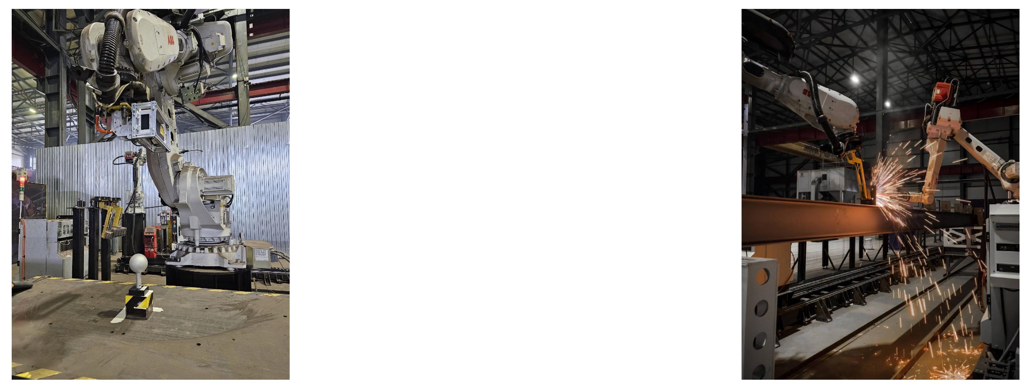
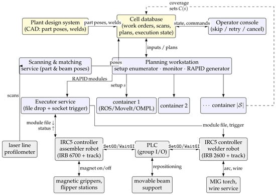
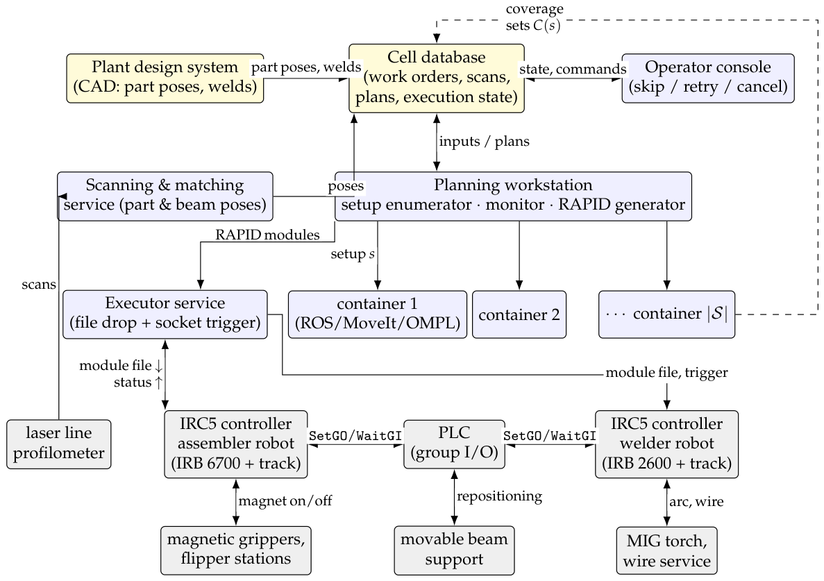
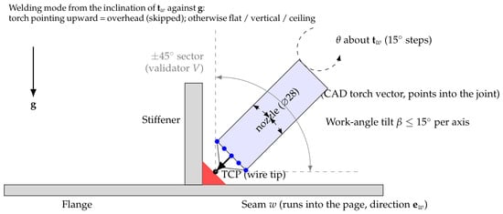
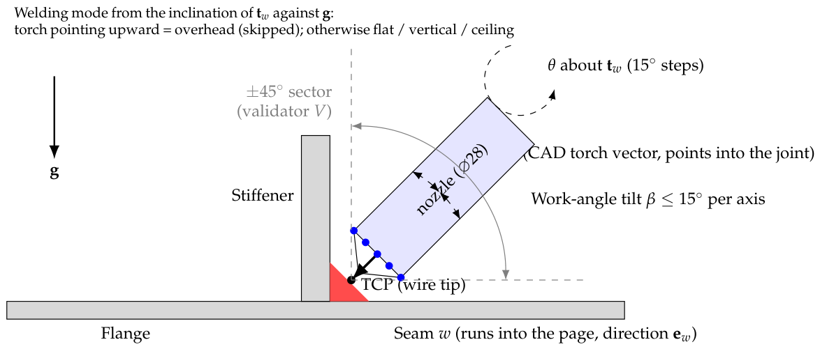
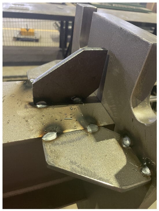
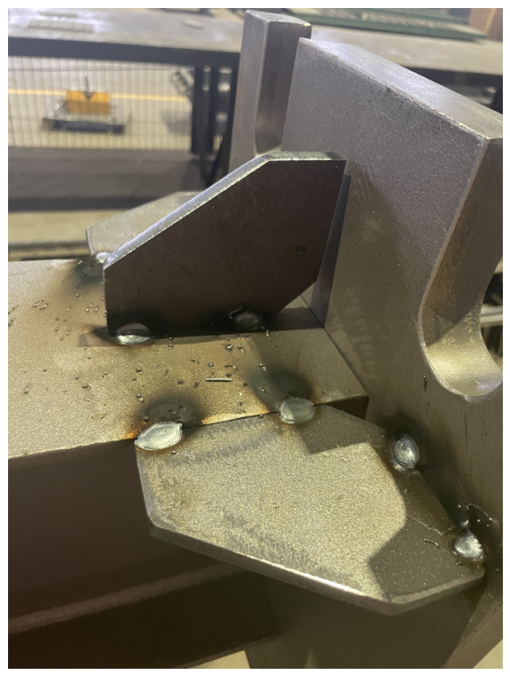
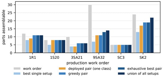
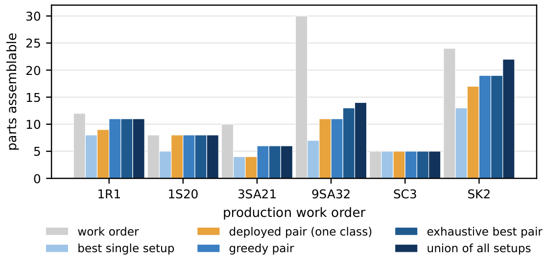

Disclaimer/Publisher’s Note: The statements, opinions and data contained in all publications are solely those of the individual author(s) and contributor(s) and not of MDPI and/or the editor(s). MDPI and/or the editor(s) disclaim responsibility for any injury to people or property resulting from any ideas, methods, instructions or products referred to in the content. |
© 2026 by the authors. Licensee MDPI, Basel, Switzerland. This article is an open access article distributed under the terms and conditions of the Creative Commons Attribution (CC BY) license.