Active Disturbance Rejection Control Combined with a Singular Perturbation Approach for Cable-Driven Parallel Robots with Elastic Cables

Abstract

Cable elasticity is the principal obstacle to accurate positioning in large cable-driven parallel robots (CDPRs). The composite controller derived from singular perturbation theory addresses it by adding a vibration-damping correction to a rigid controller, but for a machine with long and highly compliant cables, the correction must be made strong: the velocity and damping gains $K_v$ and $K_d$ have to be raised and the proportional gain $K_p$ lowered, which yields a slow and imprecise platform response. This paper augments that composite controller with active disturbance rejection control (ADRC). An extended state observer reconstructs the lumped elastic torque acting on each winch from the measured cable length, and the estimate is injected into the control law. The compensation introduces an additional tunable proportional gain $K_p^q$, which acts on the closed-loop stiffness directly, so that $K_v$ and $K_d$ can be reduced and $K_p$ increased without loss of stability, giving a faster and more accurate response. The proposed controller complements rather than replaces the composite structure: the damping correction remains necessary, and removing it destabilises the loop even when ADRC is active. Asymptotic stability of the overall closed loop is established by Lyapunov’s second method through a composite function combining the slow and fast subsystems. The controller is evaluated in simulation on the IPAnema3 spatial cable-driven parallel robot, without ADRC, with ADRC, and with ADRC under an added payload of 35 kg. Under these simulated conditions, and relative to the baseline composite controller without ADRC, the proposed controller reduces the root mean square position error by a factor of 8.2 and the integral of time-weighted absolute error by a factor of 7.7.

1. Introduction

Replacing the rigid links of a parallel manipulator with cables opens a wide range of applications, including robots with very large workspaces [1], high-speed manipulators [2], handling of heavy materials [3], intervention in disaster areas [4] and operation in remote or hazardous environments [5]. A general account of the architecture and its control is given in the survey [6]. The substitution also removes several limitations inherent to conventional parallel architectures, at the cost of one difficulty that has attracted sustained attention: a cable is not a rigid link, and its compliance acts as a flexible joint between the winch and the moving platform [7,8,9,10,11,12]. That compliance is the principal obstacle to precise platform positioning.

Several remedies have been proposed. The present work builds on the approach of Khosravi and Taghirad [7], which applies singular perturbation theory [13] to separate the slow platform motion from the fast elastic dynamics and derives a composite controller: a rigid controller designed on the reduced-order model, augmented by a corrective term that damps the fast vibration. The structure is attractive because each part has a clear role and each can be tuned separately.

The difficulty addressed here appears when this scheme is applied to a large machine such as IPAnema3 [14], whose cables are long and therefore compliant. Lower stiffness forces the designer to raise the velocity and damping gains $K_v$ and $K_d$ in order to damp the fast dynamics, and to lower the proportional gain $K_p$ in order to keep the two time scales separated. The result is a platform that positions itself slowly and imprecisely, and the composite control alone becomes inadequate.

The solution proposed here integrates active disturbance rejection control (ADRC) with the composite controller of [7]. ADRC, introduced by Han [15] and developed into its linear, bandwidth-parameterised form by subsequent work [16,17,18], treats everything that is not the nominal input as a single lumped total disturbance and reconstructs it with an extended state observer (ESO) [19]. Applied here, the ESO estimates the dynamic effect of cable elasticity and the estimate is fed back into the control law. This introduces one additional degree of freedom, the tunable proportional gain $K_p^q$, which acts on the stiffness seen by the closed loop. Because the stiffness can now be adjusted through a gain rather than accepted as a property of the cable, $K_v$ and $K_d$ can be reduced and $K_p$ increased, and the platform responds faster and more accurately. Related uses of ADRC and of observer-based compensation for elastic and vibrating mechanical systems are reported in [19,20,21].

The scheme is a complement to [7], not an alternative to it. For clarity, the remainder of this paper refers to the scheme of [7] on its own as the baseline composite controller and to the scheme developed here, which augments it with active disturbance rejection control, as the proposed controller; the term composite structure is reserved for the two-part architecture (rigid control plus elastic correction) that both controllers share. The composite structure is retained in full in the proposed controller, and the discussion following Theorem 2 in Section 3.3 shows that removing the damping correction destabilises the closed loop even when ADRC is active. The same overall strategy is followed for the stability analysis, with the ADRC contribution incorporated into the composite Lyapunov argument. The resulting improvement is quantified in Section 4.4.

The paper is organised as follows. Section 2 presents the dynamic model of the cable-driven robot with elastic cables, the equivalent rigid model, the rigid controller and its stability. Section 3 develops the ADRC in conjunction with the singular perturbation approach: the extended state observer and its convergence, the elastic dynamics, and the stability of the complete closed loop under the composite control structure. Section 4 reports the simulation study on the IPAnema3 spatial cable robot, including a quantitative comparison of the three configurations and a statement of the limitations of the work. Section 5 concludes.

2. IPAnema3 Robot with Elastic Cables

2.1. Dynamic Model

The dynamic model of the cable-driven robot IPAnema3 [14], including the effect of cable elasticity [10], is

$$\left\{\begin{array}{c}M\left(x\right)\ddot{x}+N\left(x,\dot{x}\right)=F,\hfill \\ I_m\ddot{q}+r{K}_l\left(\alpha -q\right)=u,\hfill \end{array}\right.$$

(1)

with

$$N\left(x,\dot{x}\right)=C\left(x,\dot{x}\right)\dot{x}+G\left(x\right),F=J^{\mathsf{T}}{K}_l\left(\alpha -q\right),\alpha =rq+L_0,$$

(2)

and the cable stiffness matrix

$$K_l=diag\left\{C_i\right\},C_i={\displaystyle \frac{K_{sp}}{q_i+l_{0i}}},i=1,\dots ,8.$$

(3)

Here $x\in {\mathbb{R}}^6$ is the vector of generalised coordinates of the platform, $M\left(x\right)\in {\mathbb{R}}^{6\times 6}$ the symmetric positive-definite inertia matrix, $C(x,\dot{x})\in {\mathbb{R}}^{6\times 6}$ the matrix of Coriolis and centrifugal effects, $G\left(x\right)\in {\mathbb{R}}^6$ the vector of gravitational forces, and $u\in {\mathbb{R}}^8$ the vector of motor torques. The vector $q\in {\mathbb{R}}^8$ is the length of the tensioned cable, obtained from the inverse kinematics or measured with a string potentiometer, and $\alpha \in {\mathbb{R}}^8$ is the actuator-side cable length, obtained from the motor shaft encoder. The quantity F is the wrench that the cables exert on the moving platform, $L_0$ the vector of cable lengths at $x=0$, $I_m$ the diagonal matrix of winch inertias, $l_{0i}$ the unconstrained length of cable i between the drum and the final pulley, and J the Jacobian matrix of the mechanism.

Two points of notation are worth stating explicitly, since both were sources of ambiguity in earlier presentations of this model.

Notation 1. 

The symbol r in (1) and (2) is the dimensionless transmission ratio of the winch, not a length. It is distinct from the pulley radii $r_{p,i}$ listed in Table 1, which are expressed in millimetres and enter only the kinematic construction of the pulley contact points. With r dimensionless, the relation $\alpha =rq+L_0$ is dimensionally homogeneous, all three terms being lengths.

Table 1. Geometric parameters of the IPAnema3 robot. Base anchor points $a_i$ are expressed in the world frame and platform anchor points $b_i$ in the platform frame, both in metres. The pulley orientation ${\phi }_{A,i}$ is given as an intrinsic XYZ Euler triple $(\alpha ,\beta ,\gamma )$ in degrees, $r_{p,i}$ is the pulley radius and $l_{0i}$ is the drum-to-pulley cable length.

Cable	Base Anchor ${\mathit{a}}_{\mathit{i}}$ [m]				Platform Anchor ${\mathit{b}}_{\mathit{i}}$ [m]				Pulley Orientation ${\mathit{\phi }}_{\mathit{A},\mathit{i}}$ [deg]			${\mathit{r}}_{\mathit{p},\mathit{i}}$	${\mathit{l}}_{0\mathit{i}}$
$\mathit{i}$	$\mathit{x}$	$\mathit{y}$	$\mathit{z}$		$\mathit{x}$	$\mathit{y}$	$\mathit{z}$		$\mathit{\alpha }$	$\mathit{\beta }$	$\mathit{\gamma }$	[mm]	[m]
1	8.185	5.693	3.203		0.061	0.649	−0.261		90	0	−90	52.0	4.6
2	8.224	−5.492	3.236		0.061	−0.651	−0.261		90	0	90	52.0	4.6
3	−8.491	−5.322	3.250		−0.070	−0.652	−0.261		90	0	90	52.0	4.5
4	−8.545	5.464	3.221		−0.070	0.648	−0.261		90	0	−90	52.0	4.3
5	7.208	6.464	−0.590		0.095	0.749	0.261		90	0	−90	35.0	0.3
6	7.869	−5.558	−0.549		0.095	−0.746	0.261		−90	180	0	35.0	0.3
7	−8.271	−5.546	−0.583		−0.086	−0.746	0.262		90	0	90	35.0	0.3
8	−8.192	5.648	−0.583		−0.086	0.749	0.262		−90	0	180	35.0	0.3

Notation 2. 

The symbol q denotes the winch-side cable coordinate, that is, the state integrated from the actuator equation in (1), throughout Section 2 and Section 4. It is related to the actuator-side length by $\alpha =rq+L_0$ and is not identical to the geometric distance between the base and platform anchor points, so its numerical range in the results of Section 4.3 is not bounded by the physical span of the machine. The internal states of the extended state observer introduced in Section 3.1 are written $q_1$, $q_2$ and $q_3$, and their estimates ${\widehat{z}}_1$, ${\widehat{z}}_2$ and ${\widehat{z}}_3$. A complete list of symbols with units is given in the Nomenclature.

Assumption 1. 

The present study analyses the interaction between the rigid platform dynamics and the elastic cable dynamics, and the platform is not subjected to gravitational loading in the simulation model of Section 4; the gravity vector $G\left(x\right)$ is retained in the analytical development of Section 2 and Section 3 but is set to zero in the numerical study so that the response observed is attributable to the elastic dynamics alone rather than to the static load distribution. Including gravitational loading of the platform requires a corresponding increase in the cable pretension and in the specific stiffness $K_{sp}$, and is left to future work. The payload case of Section 4.3 is therefore to be read as a perturbation of the inertial parameters and of the applied wrench, introduced through the term $w_0$ of the platform force balance, rather than as a full static loading of the mechanism.

This restriction concerns the numerical case study alone, not the control law or its stability guarantee. Substituting the rigid control law of Section 2.2 into the equivalent model of the same section gives the closed-loop dynamics of Section 2.3, in which $G_{eq}\left(x\right)$ does not appear at all: it is cancelled exactly by the feedforward term $G_{eq}\left(x\right)$ already present in the rigid control law, for every value of $G\left(x\right)$ and hence for every level of gravitational loading. The proof of Lemma 1 accordingly makes no reference to the magnitude of $G\left(x\right)$. Assumption 1 therefore restricts the fidelity of the simulated plant in Section 4, not the applicability of the control law developed in Section 2 and Section 3, which is gravity-independent by construction.

$K_{sp}$ is the specific stiffness of the cable. Taking the nonlinearity of the cable material into account, the specific stiffness depends on the actual cable force and is modelled in [14] as a second-degree polynomial,

$$K_{sp}=k_0+k_{1}f+k_2{f}^2,f>0,$$

(4)

where f is the cable force. The constant value reported in Table 2 is the value used throughout the present study.

Table 2. Dynamic, drive-train and numerical parameters used in the simulation. The initial cable lengths are $L_0={[10.084,9.875,10.095,10.194,9.265,9.239,9.599,9.570]}^{\mathsf{T}}$ m, computed from the initial pose $x_0$ by inverse kinematics.

Symbol	Description	Value	Unit
$m_p$	Platform mass	30	kg
$m_{pl}$	Additional payload (load case only)	35	kg
$C_{m_{p,0}}$	Platform centre of mass	${10}^{-3}{\left[-0.5,0.5,408.8\right]}^{\mathsf{T}}$	m
$J_C$	Platform inertia tensor	$diag\left(0.251,0.258,0.073\right)$	kg·m2
$K_{sp}$	Specific cable stiffness	900	N
$I_m$	Winch inertia matrix	$4.562\times {10}^{-3}{I}_{8\times 8}$	kg·m2
r	Winch transmission ratio	$4.338\times {10}^{-3}$	–
$x_0$	Initial platform pose	${\left[0,0,0.5,0,0,0\right]}^{\mathsf{T}}$	m, rad
${\omega }_0$	Observer bandwidth	350	rad·s−1
–	Solver	ode14x, extrapolation order 1	–
–	Fixed step size	$0.01$	s
–	Simulation duration, with ADRC	30	s
–	Simulation duration, without ADRC	40	s

The choice between the constant approximation and the tension-dependent form (4) affects only the fidelity of the simulated plant, not the applicability of the compensation proposed in Section 3. The extended state observer of Section 3.1 reconstructs the lumped torque $f_q=r{K}_l(\alpha -q)$ directly from the measured cable length q, and neither the observer equations nor the convergence result of Theorem 1 make any assumption on the functional form of $K_l$: Theorem 1 requires only the bound $|{\dot{f}}_q|\le M_{fq}$ on the rate of change of the total disturbance, a condition that $K_l$ constant and $K_l$ given by (4) satisfy equally over a bounded trajectory. The same observer and the same convergence guarantee therefore apply whether the true cable stiffness is constant or tension-dependent; the constant-$K_l$ assumption is a property of the case study used to illustrate the method in Section 4, not a restriction the method itself imposes.

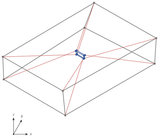
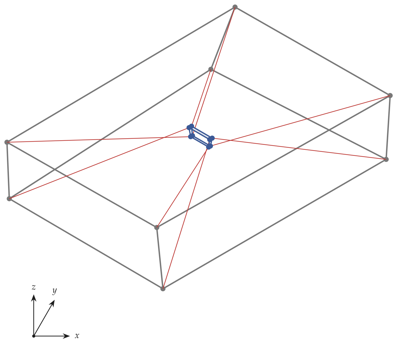
The IPAnema3 cable-driven parallel robot, developed at the Fraunhofer Institute for Manufacturing Engineering and Automation (IPA), Stuttgart, Germany, is designed for material handling, load manipulation and tasks requiring precision together with a large working volume. Its architecture combines a wide workspace with a high payload-to-mass ratio, which is what makes cable compliance the limiting factor on accuracy and therefore the subject of this work. The frame and cable configuration of the robot are shown schematically in Figure 1.

Figure 1. Schematic representation of the IPAnema3 cable-driven parallel robot, drawn from the geometric data of Table 1: the eight base anchor points and the gantry frame connecting them (grey), the eight cables at a representative platform pose $x={[0,0,2,0,0,0]}^{\mathsf{T}}$ m (red), and the moving platform they support (blue). The world frame is located at the geometric centre of the base anchor points with the z axis vertical, as shown by the triad at bottom left; the platform frame is attached at the geometric centre of the platform anchor points. This is an original illustration generated from the authors’ own numerical data and does not reproduce any previously published image.

2.2. Control of the Rigid Structure

Consider the equivalent dynamic model of the cable-driven robot that incorporates cable elasticity, as described in [10],

$$\left\{\begin{array}{c}{M}_{eq}\left(x\right)\ddot{x}+N_{eq}\left(x,\dot{x}\right)=J^{\mathsf{T}}{u}_r,\hfill \\ M_{eq}\left(x\right)=rM\left(x\right)+r^{-1}{J}^{\mathsf{T}}{I}_{m}J,\hfill \\ N_{eq}\left(x,\dot{x}\right)=C_{eq}\left(x,\dot{x}\right)\dot{x}+G_{eq}\left(x\right),\hfill \\ C_{eq}\left(x,\dot{x}\right)\dot{x}=rC\left(x,\dot{x}\right)\dot{x}+r^{-1}{J}^{\mathsf{T}}{I}_m\dot{J}\dot{x},\hfill \\ G_{eq}\left(x\right)=rG\left(x\right).\hfill \end{array}\right.$$

(5)

This form is convenient both for designing the rigid controller and for constructing the extended state observer of Section 3.1.

The rigid control law, following [7], is

$$u_r=J^{†}\left(M_{eq}\left(x\right){\ddot{x}}_d+C_{eq}\left(x,\dot{x}\right){\dot{x}}_d+G_{eq}\left(x\right)+K_p\left(x_d-x\right)+K_v\left({\dot{x}}_d-\dot{x}\right)\right)+\mathcal{Q},$$

(6)

where $K_p$ and $K_v$ are diagonal matrices of positive gains, and $J^{†}=J{\left(J^{\mathsf{T}}J\right)}^{-1}$ is the Moore–Penrose pseudoinverse of $J^{\mathsf{T}}$.

The vector $\mathcal{Q}$ lies in the null space of $J^{\mathsf{T}}$ so that $J^{\mathsf{T}}\mathcal{Q}=0$. It therefore generates internal forces in the cables without affecting the motion of the platform, and its magnitude is chosen so that every cable remains in tension over the whole trajectory. This term is essential: a cable can only pull, and the control is meaningful only while all tensions remain strictly positive. The magnitude of the commanded cable forces realised in simulation is reported in Section 4.3.

2.3. Stability of the Rigid Body Dynamics

Substituting (6) into (5) gives the closed-loop error dynamics

$$M_{eq}\left(x\right)\ddot{e}+C_{eq}\left(x,\dot{x}\right)\dot{e}+K_v\dot{e}+K_{p}e=0,e=x_d-x.$$

(7)

Lemma 1. 

For diagonal positive-definite gain matrices $K_p$ and $K_v$, the equilibrium $e=0$, $\dot{e}=0$ of the closed-loop system (7) is asymptotically stable.

Proof. 

Consider the Lyapunov function candidate

$$V_R=\frac{1}{2}{\dot{e}}^{\mathsf{T}}{M}_{eq}\left(x\right)\dot{e}+\frac{1}{2}{e}^{\mathsf{T}}{K}_{p}e.$$

(8)

Since $M_{eq}\left(x\right)$ is symmetric positive definite and $K_p$ is positive definite, $V_R>0$ for all $(e,\dot{e})\ne (0,0)$ and $V_R=0$ only at the origin. Differentiating along the trajectories of (7),

$${\dot{V}}_R={\dot{e}}^{\mathsf{T}}{M}_{eq}\ddot{e}+\frac{1}{2}{\dot{e}}^{\mathsf{T}}{\dot{M}}_{eq}\dot{e}+{\dot{e}}^{\mathsf{T}}{K}_{p}e,$$

and substituting $M_{eq}\ddot{e}=-C_{eq}\dot{e}-K_v\dot{e}-K_{p}e$ from (7),

$${\dot{V}}_R=\frac{1}{2}{\dot{e}}^{\mathsf{T}}\left({\dot{M}}_{eq}-2C_{eq}\right)\dot{e}-{\dot{e}}^{\mathsf{T}}{K}_v\dot{e}.$$

The matrix ${\dot{M}}_{eq}-2C_{eq}$ is skew symmetric, so the first term vanishes and

$${\dot{V}}_R=-{\dot{e}}^{\mathsf{T}}{K}_v\dot{e}\le 0.$$

(9)

Thus ${\dot{V}}_R$ is negative semi-definite and vanishes only on the set $\{\dot{e}=0\}$. Since $V_R$ is radially unbounded, e and $\dot{e}$ remain bounded; hence, $\ddot{e}$ is bounded and ${\dot{V}}_R$ is uniformly continuous. Barbalat’s lemma then gives $\dot{e}\to 0$, and substituting back into (7) leaves $K_{p}e\to 0$, that is $e\to 0$. The equilibrium is therefore asymptotically stable. □

3. ADRC Based on the Singular Perturbation Method

3.1. Extended State Observer and Its Convergence

The dynamics selected for compensation are those of the cable subsystem. Define the observer states

$$q_1=q,q_2=\dot{q},q_3=f_q,$$

(10)

where the total disturbance, that is, the lumped elastic torque acting on the winch, is

$$f_q=r{K}_l\left(\alpha -q\right),{\widehat{h}}_q={\dot{f}}_q.$$

(11)

Lumping the elastic coupling into a single quantity in this way is what allows the winch subsystem to be written in the chain-of-integrators form required by ADRC. The augmented state-space representation of the second equation of (1) is then exact, not approximate:

$$\left\{\begin{array}{c}{\dot{q}}_1=q_2,\hfill \\ {\dot{q}}_2=-I_m^{-1}{f}_q+I_m^{-1}{u}_q,\hfill \\ {\dot{q}}_3={\widehat{h}}_q.\hfill \end{array}\right.$$

(12)

The only signal required for the observer is the cable length q, which is measured directly.

The extended state observer that reconstructs these states and the unmeasured lumped disturbance is

$$\left\{\begin{array}{c}{\dot{\widehat{z}}}_1={\widehat{z}}_2-{\alpha }_1{e}_q,\hfill \\ {\dot{\widehat{z}}}_2=-I_m^{-1}{\widehat{z}}_3+I_m^{-1}{u}_q-{\alpha }_2{e}_q,\hfill \\ {\dot{\widehat{z}}}_3={\alpha }_3{e}_q,\hfill \end{array}\right.e_q={\widehat{z}}_1-q_1,{\alpha }_i>0.$$

(13)

The gains ${\alpha }_i$ are designed so that the estimated states converge to the actual states, with the accuracy and robustness required under varying dynamics and external disturbance.

The control law that stabilises these dynamics and uses the observer estimate is

$$u_q={\widehat{z}}_3,$$

(14)

so that the estimated elastic torque is fed back to cancel the true one.

Following the bandwidth parameterisation of ADRC, all three observer poles are placed at $-{\omega }_0$. Writing ${\tilde{q}}_i={\widehat{z}}_i-q_i$ and subtracting (12) from (13), the estimation error obeys

$$\dot{\tilde{q}}=A_o\tilde{q}-B_o{\dot{f}}_q,A_o=\left[\begin{array}{ccc}-{\alpha }_1& 1& 0\\ -{\alpha }_2& 0& -I_m^{-1}\\ {\alpha }_3& 0& 0\end{array}\right],B_o=\left[\begin{array}{c}0\\ 0\\ 1\end{array}\right],$$

(15)

whose characteristic polynomial is $s^3+{\alpha }_1{s}^2+{\alpha }_{2}s+{\alpha }_3{I}_m^{-1}$. Matching it to the desired polynomial,

$$s^3+{\alpha }_1{s}^2+{\alpha }_{2}s+{\alpha }_3{I}_m^{-1}={\left(s+{\omega }_0\right)}^3,$$

(16)

gives the observer gains

$${\alpha }_1=3{\omega }_0,{\alpha }_2=3{\omega }_0^2,{\alpha }_3=I_m{\omega }_0^3.$$

(17)

A single parameter ${\omega }_0$ therefore tunes the observer. Its selection is a compromise between estimation accuracy and noise rejection: a larger ${\omega }_0$ accelerates convergence and tightens the estimate, but amplifies measurement noise, since the gain from the measured cable length to ${\widehat{z}}_3$ grows as ${\omega }_0^3$. In the present study the cable length and platform pose measurements are assumed free of noise, so ${\omega }_0$ is chosen large in order to maximise estimation accuracy.

Theorem 1. 

Assume the derivative of the total disturbance is bounded, that is, $\left|{\dot{f}}_q\right|\le M_{fq}$ for some $M_{fq}>0$. Then, with the gains (17), the error dynamics (15) are exponentially stable and the estimation error converges to a residual set whose size is proportional to $M_{fq}$ and decreases as the observer bandwidth ${\omega }_0$ increases. In particular, if ${\dot{f}}_q\to 0$ then $\tilde{q}\to 0$ exponentially.

Proof. 

By the pole assignment (16) and (17) the eigenvalues of $A_o$ are located at $-{\omega }_0$ with multiplicity three, so $A_o$ is Hurwitz for every ${\omega }_0>0$. There exists therefore a symmetric positive-definite matrix P solving the Lyapunov equation $A_o^{\mathsf{T}}P+P{A}_o=-I$. Taking $V_o={\tilde{q}}^{\mathsf{T}}P\tilde{q}$ and differentiating along (15),

$${\dot{V}}_o=-{∥\tilde{q}∥}^2-2{\tilde{q}}^{\mathsf{T}}P{B}_o{\dot{f}}_q\le -{∥\tilde{q}∥}^2+2∥P{B}_o∥M_{fq}∥\tilde{q}∥.$$

Hence ${\dot{V}}_o<0$ whenever $∥\tilde{q}∥>2∥P{B}_o∥M_{fq}$, which establishes exponential convergence to a residual ball of radius proportional to $M_{fq}$. If ${\dot{f}}_q\to 0$ the perturbation term vanishes and ${\dot{V}}_o\le -{\parallel \tilde{q}\parallel }^2$, giving exponential convergence to the origin. □

3.2. Analysis of the Elastic Dynamics

The complete stability argument of [7] is not repeated here; only the steps that differ through the introduction of ADRC are developed. The equations of motion, incorporating both the rigid and the elastic components, are

$$\left\{\begin{array}{c}M\left(x\right)\ddot{x}+N\left(x,\dot{x}\right)=J^{\mathsf{T}}K\left(\alpha -q\right),\hfill \\ I_m\ddot{q}+f_q=u,\hfill \end{array}\right.$$

(18)

with $f_q=r{K}_l(\alpha -q)$ the term governing cable flexibility, which is the quantity compensated by ADRC.

The proposed control law combines the ADRC contribution with the baseline composite controller of [7],

$$u=u_r+u_q+K_p^q\left(q-\alpha \right)+K_d\left(\dot{q}-\dot{\alpha }\right),$$

(19)

where $u_q$ is given by (14) and $u_r$ by (6). Following [7], set

$$\alpha =rq+L_0,z=K\left(\alpha -q\right),$$

(20)

and introduce the singular perturbation parameter $\epsilon$ through

$$K={\displaystyle \frac{K_1}{{\epsilon }^2}},K_d={\displaystyle \frac{K_2}{\epsilon }},K_p^q=K_1.$$

(21)

The closed-loop dynamics determined by (19) then take the singularly perturbed form

$$\left\{\begin{array}{c}M\left(x\right)\ddot{x}+C\left(x,\dot{x}\right)\dot{x}+G\left(x\right)=J^{\mathsf{T}}z,\hfill \\ {\epsilon }^2{r}^{-1}{I}_m\ddot{z}+\epsilon K_2\dot{z}+r{K}_{1}z-{\tilde{q}}_3=K_1\left(u_r-r^{-1}{I}_m\ddot{q}\right),\hfill \end{array}\right.$$

(22)

where

$${\tilde{q}}_3={\widehat{z}}_3-q_3={\widehat{z}}_3-f_q$$

(23)

is the estimation error of the flexible dynamics, that is, the residual left by the observer.

Introducing the fast time scale $\tau =t/\epsilon$ and the fast state variable $\eta$ obeying the boundary-layer equation, as in [7], the equivalent elastic system is

$$r^{-1}{I}_m{\displaystyle \frac{d^2\eta }{d{\tau }^2}}+K_2{\displaystyle \frac{d\eta }{d\tau }}+r{K}_1\eta ={\tilde{q}}_3,$$

(24)

and the complete singularly perturbed model reads

$$\left\{\begin{array}{c}{M}_{eq}\left(x\right)\ddot{x}+C_{eq}\left(x,\dot{x}\right)\dot{x}+G_{eq}\left(x\right)=J^{\mathsf{T}}\left(u_r+r\eta \left(\tau \right)\right),\hfill \\ r^{-1}{I}_m{\displaystyle \frac{d^2\eta }{d{\tau }^2}}+K_2{\displaystyle \frac{d\eta }{d\tau }}+r{K}_1\eta ={\tilde{q}}_3.\hfill \end{array}\right.$$

(25)

The gains $K_1$ and $K_2$ can be chosen so that the boundary-layer system (24) is asymptotically stable, as shown in [7]. The condition on the forcing term is that ${\tilde{q}}_3$ approach zero rapidly so that the residual left by the observer does not sustain the fast oscillation. This is guaranteed by the exponential convergence established in Theorem 1: the observer operates inside the feedback loop, provides a continuously updated estimate of the elastic torque, and keeps the residual within a bound that shrinks with the observer bandwidth. With $K_1$ and $K_2$ chosen accordingly, the boundary-layer system attains the required asymptotic stability.

3.3. Stability of the Complete System

Combining (25) with the rigid control law (6), the closed-loop dynamics are

$$\left\{\begin{array}{c}{M}_{eq}\left(x\right)\ddot{e}+\left(C_{eq}\left(x,\dot{x}\right)+K_v\right)\dot{e}+K_{p}e=-r{J}^{\mathsf{T}}\eta \left(t/\epsilon \right),\hfill \\ r^{-1}{I}_m\ddot{\eta }+K_d\dot{\eta }+r{K}_1\eta ={\tilde{q}}_3,\hfill \end{array}\right.$$

(26)

which in two-time-scale state form become

$$\dot{y}=Ay+B\left[\begin{array}{cc}I& 0\end{array}\right]h,\dot{h}=\overline{A}h+D,$$

(27)

with

$$y=\left[\begin{array}{c}e\\ \dot{e}\end{array}\right],e=x_d-x,h=\left[\begin{array}{c}\eta \\ \dot{\eta }\end{array}\right],$$

(28)

$$\overline{A}=\left[\begin{array}{cc}0& I\\ -r^2{I}_m^{-1}{K}_1& -r{I}_m^{-1}{K}_d\end{array}\right],D=\left[\begin{array}{c}0\\ r{I}_m^{-1}{\tilde{q}}_3\end{array}\right],$$

(29)

the matrices A and B being those given in [7].

Lemma 2. 

There exist positive-definite matrices $K_p^q$ and $K_d$ such that, given an accurate estimate of $f_q$, the fast subsystem (27) is asymptotically stable.

Proof. 

Let $a=r^{-1}{I}_m$ and take the Lyapunov function candidate

$$V_F=\frac{1}{2}{\dot{\eta }}^{\mathsf{T}}a\dot{\eta }+\frac{1}{2}{\eta }^{\mathsf{T}}{K}_1\eta +\sigma {\eta }^{\mathsf{T}}\dot{\eta },$$

(30)

which is positive definite provided the scalar $\sigma >0$ satisfies ${\sigma }^2<{\lambda }_{min}\left(a\right){\lambda }_{min}\left(K_1\right)$. Using $a\ddot{\eta }=-K_d\dot{\eta }-r{K}_1\eta +{\tilde{q}}_3$ from (26) and differentiating,

$${\dot{V}}_F=-{\dot{\eta }}^{\mathsf{T}}\left(K_d-\sigma I\right)\dot{\eta }-\sigma r{\eta }^{\mathsf{T}}{a}^{-1}{K}_1\eta -\sigma {\eta }^{\mathsf{T}}{a}^{-1}{K}_d\dot{\eta }+{\left(\dot{\eta }+\sigma a^{-1}\eta \right)}^{\mathsf{T}}{\tilde{q}}_3,$$

which can be written compactly as

$${\dot{V}}_F=-h^{\mathsf{T}}Sh+{\left(\dot{\eta }+\sigma a^{-1}\eta \right)}^{\mathsf{T}}{\tilde{q}}_3,S=\left[\begin{array}{cc}\sigma r{a}^{-1}{K}_1& \frac{1}{2}\sigma a^{-1}{K}_d\\ \frac{1}{2}\sigma a^{-1}{K}_d& K_d-\sigma I\end{array}\right].$$

(31)

Since $K_1=K_p^q$ and $K_d$ are positive definite and $\sigma <{\lambda }_{min}\left(K_d\right)$, the Schur complement condition

$${\lambda }_{min}\left(K_1\right)>{\displaystyle \frac{\sigma {\lambda }_{max}^2\left(K_d\right)}{4r{\lambda }_{min}\left(a\right)\left({\lambda }_{min}\left(K_d\right)-\sigma \right)}}$$

(32)

makes S positive definite. Given that ${\tilde{q}}_3\to 0$ after a short transient by Theorem 1, the forcing term vanishes and ${\dot{V}}_F=-h^{\mathsf{T}}Sh$ is negative definite. Hence $h\to 0$ and the fast subsystem is asymptotically stable. □

Every term in (30) to (32) is dimensionally homogeneous, a having the units of a rotational inertia divided by the transmission ratio, $K_1$ those of a stiffness and $\sigma$ those of a damping coefficient.

Theorem 2. 

The closed-loop system described by (27) is asymptotically stable, through appropriate selection of the controller gains $K_v$, $K_p^q$ and $K_d$ together with compensation of the elastic dynamics by ADRC.

Proof. 

Take the composite Lyapunov function candidate of [7],

$$V(y,h)=V_R+\varrho V_F,\varrho >0,$$

(33)

with $V_R$ from (8) and $V_F$ from (30), both positive definite. Differentiating along (27) and combining the coupling term $-r{J}^{\mathsf{T}}\eta$ of (26) with (31),

$$\dot{V}(y,h)=-{\dot{e}}^{\mathsf{T}}{K}_v\dot{e}-r{\dot{e}}^{\mathsf{T}}{J}^{\mathsf{T}}\eta -\varrho h^{\mathsf{T}}Sh+\varrho {\left(\dot{\eta }+\sigma a^{-1}\eta \right)}^{\mathsf{T}}{\tilde{q}}_3.$$

(34)

Bounding each quadratic form by its extreme eigenvalue and the coupling term by the largest singular value of $J^{\mathsf{T}}$,

$$\dot{V}(y,h)\le -{\left[\begin{array}{c}∥\dot{e}∥\\ ∥h∥\end{array}\right]}^{\mathsf{T}}\left[\begin{array}{cc}{\lambda }_{min}\left(K_v\right)& -\frac{1}{2}r{\sigma }_{max}\left(J^{\mathsf{T}}\right)\\ -\frac{1}{2}r{\sigma }_{max}\left(J^{\mathsf{T}}\right)& \varrho {\lambda }_{min}\left(S\right)\end{array}\right]\left[\begin{array}{c}∥\dot{e}∥\\ ∥h∥\end{array}\right]+\varrho {\left(\dot{\eta }+\sigma a^{-1}\eta \right)}^{\mathsf{T}}{\tilde{q}}_3.$$

If ${\tilde{q}}_3$ vanishes after a short period under the action of ADRC, and if $K_v$ in (6) together with $K_p^q$ and $K_d$ for the fast subsystem are chosen so that the two-by-two matrix above is positive definite, that is

$${\lambda }_{min}\left(K_v\right)\varrho {\lambda }_{min}\left(S\right)>\frac{1}{4}{r}^2{\sigma }_{max}^2\left(J^{\mathsf{T}}\right),$$

(35)

then $\dot{V}(y,h)\le 0$. Applying Barbalat’s lemma as in the previous analyses completes the proof of asymptotic stability of the complete closed loop. The gains $K_p$ and $K_v$ follow from the stability conditions of the rigid-body model in Lemma 1, while $K_p^q$, $K_d$ and $K_v$ must additionally satisfy (32) and (35). The pair $K_p^q$ and $K_d$ governs the rapid damping of the oscillations induced by the fast dynamics $\eta \left(t\right)$ [7]. □

Remark 1. 

The three assumptions of [7] are retained. In addition, compensating the elastic dynamics through ADRC improves the damping of the oscillations and therefore both the speed and the precision of the response, particularly for systems with long cables. By adjusting $K_p^q$, the stiffness acting in the closed loop is increased without raising $K_v$ and $K_d$, which matters because raising those gains constrains both the achievable performance and the usable workspace of the robot.

Remark 2. 

The control law (14) is an internal mechanism that stabilises the extended state observer, and forms an integral part of the overall control strategy rather than a separate loop.

An important structural consequence of the ADRC formulation deserves emphasis. In contrast to [7], the time derivative of the composite Lyapunov function no longer contains the physical stiffness K. It is replaced by the freely chosen gain $K_p^q$, which removes the need to increase $K_v$ and $K_d$ in order to damp the oscillations. As a result $K_p$ can be increased, improving the speed of response without compromising stability.

Despite this relaxation, the composite structure of [7] remains a necessary component. Removing the corrective term $K_d(\dot{q}-\dot{\alpha })$ makes the overall closed loop unstable even when ADRC is active, because setting $K_d=0$ renders S in (31) singular and (35) unsatisfiable. Cancelling the elastic torque removes the restoring action but not the winch inertia, and the damping term is what remains to dissipate the resulting oscillation. This result also bears on the choice of baseline for the comparison in Section 4: a rigid controller that ignores cable elasticity entirely corresponds to the limiting case $K_d=0$ and $K_p^q=0$ in (19), which the preceding argument shows to be unstable by the same mechanism, so such a controller could not be expected to track the trajectories of Section 4.2 on a machine with the cable compliance considered here. The composite controller of [7], which retains $K_d$ but not the ADRC term, is the least restrictive controller for which the closed loop is stable, and is therefore adopted as the comparison in Section 4 so that the contribution of $K_p^q$ can be isolated from the contribution of the damping correction itself. This is why the proposed controller is presented throughout as a complement to the baseline composite controller rather than a replacement for it.

4. Case Study: The IPAnema3 Spatial Cable Robot

4.1. Robot Parameters

The proposed framework is evaluated on the cable-driven robot IPAnema3, whose geometry is documented by Kraus [14]. Table 1 lists the base and platform anchor points, the pulley orientations, the pulley radii and the drum-to-pulley cable lengths. These parameters determine the kinematic and dynamic behaviour of the mechanism and are required to reproduce the results reported below.

The platform inertia matrix and the nonlinear term are

$$M\left(x\right)=\left[\begin{array}{cc}{m}_p{I}_3& -m_p\left[C_{m_p}\right]\\ m_p\left[C_{m_p}\right]& J_C-m_p\left[C_{m_p}\right]\left[C_{m_p}\right]\end{array}\right],N\left(x,\dot{x}\right)=\left[\begin{array}{c}{m}_p\dot{\phi }\times \left(\dot{\phi }\times C_{m_p}\right)\\ \dot{\phi }\times \left(J_C-m_p\left[C_{m_p}\right]\left[C_{m_p}\right]\right)\dot{\phi }\end{array}\right],$$

(36)

where $C_{m_p}$ is the centre of mass of the platform and $\left[C_{m_p}\right]$ the associated skew-symmetric matrix. When additional masses are carried, the combined centre of mass is

$$C_{m_p}={\displaystyle \frac{m_{p,0}{C}_{m_{p,0}}+m_1{C}_{m_1}+m_2{C}_{m_2}}{m_{p,0}+m_1+m_2}}.$$

(37)

The dynamic, drive-train and numerical parameters used in the simulation are collected in Table 2. The simulations were run in MATLAB R2014a (The MathWorks, Inc., Natick, MA, USA).

The controller gains for the three cases studied are listed in Table 3. Grouping them in a single table makes the comparison explicit: the case without ADRC requires a low proportional gain together with large velocity and damping gains, whereas the introduction of $K_p^q$ permits the opposite balance.

Table 3. Controller and observer gains for the three simulated cases.

Gain	Without ADRC	With ADRC	With ADRC and Payload
$K_p$	$1200I_{6\times 6}$	$3500I_{6\times 6}$	$3500I_{6\times 6}$
$K_v$	15,000 $I_{6\times 6}$	11,000 $I_{6\times 6}$	25,000 $I_{6\times 6}$
$K_d$	25,500 $I_{8\times 8}$	200 $I_{8\times 8}$	$700I_{8\times 8}$
$K_p^q$	–	$100I_{8\times 8}$	$50I_{8\times 8}$
${\omega }_0$	–	350	350
$m_{pl}$	0	0	35 kg

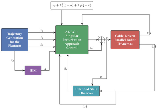
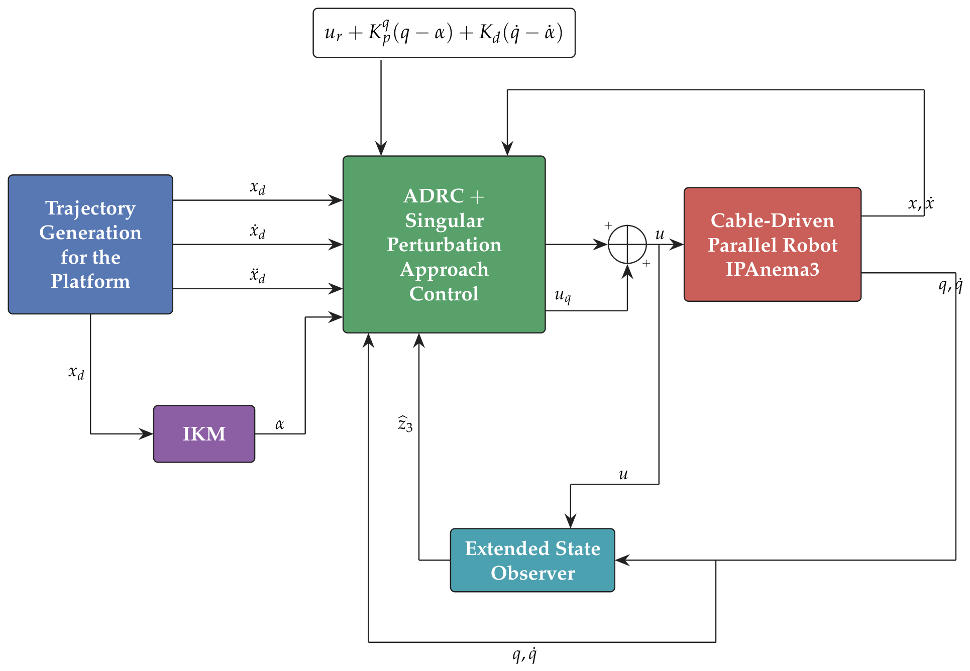
The complete control strategy implemented in the closed loop is shown in Figure 2.

Figure 2. Block diagram of the complete control strategy. The outer loop computes the rigid control $u_r$ from the pose error; the extended state observer reconstructs the lumped elastic torque $f_q$ from the measured cable length q; and the composite correction $K_p^q(q-\alpha )+K_d(\dot{q}-\dot{\alpha })$ damps the fast elastic dynamics. Measured signals are the cable lengths q and the platform pose x.

4.2. Reference Trajectory

The simulation is executed with the following continuous reference trajectories in the task-space coordinate system:

$$\left\{\begin{array}{c}{x}_d=y_d=3+1.5e^{-t}-1.8e^{-t/1.2},\hfill \\ z_d=4+e^{-t}-1.2e^{-t/1.2},\hfill \\ {\psi }_d={\theta }_d=0,{\phi }_d=4+e^{-t}-1.2e^{-t/1.2}.\hfill \end{array}\right.$$

(38)

Each channel starts from its initial value and settles smoothly to a constant, so the trajectory exercises the transient response of the controller, which is where the elastic dynamics are most strongly excited.

4.3. Results and Discussion

4.3.1. Composite Control Without ADRC

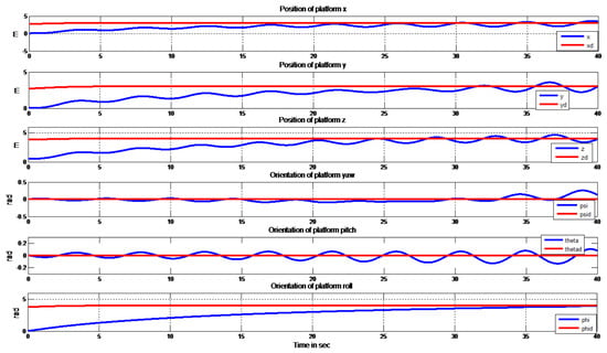
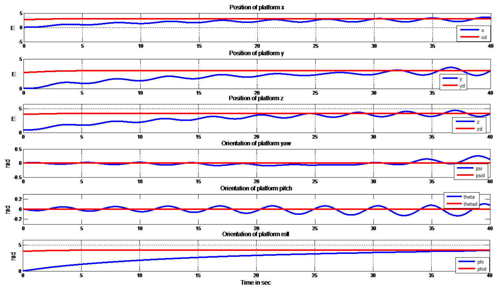
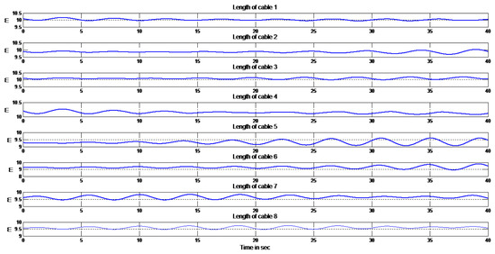
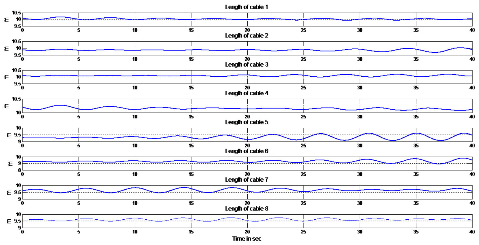
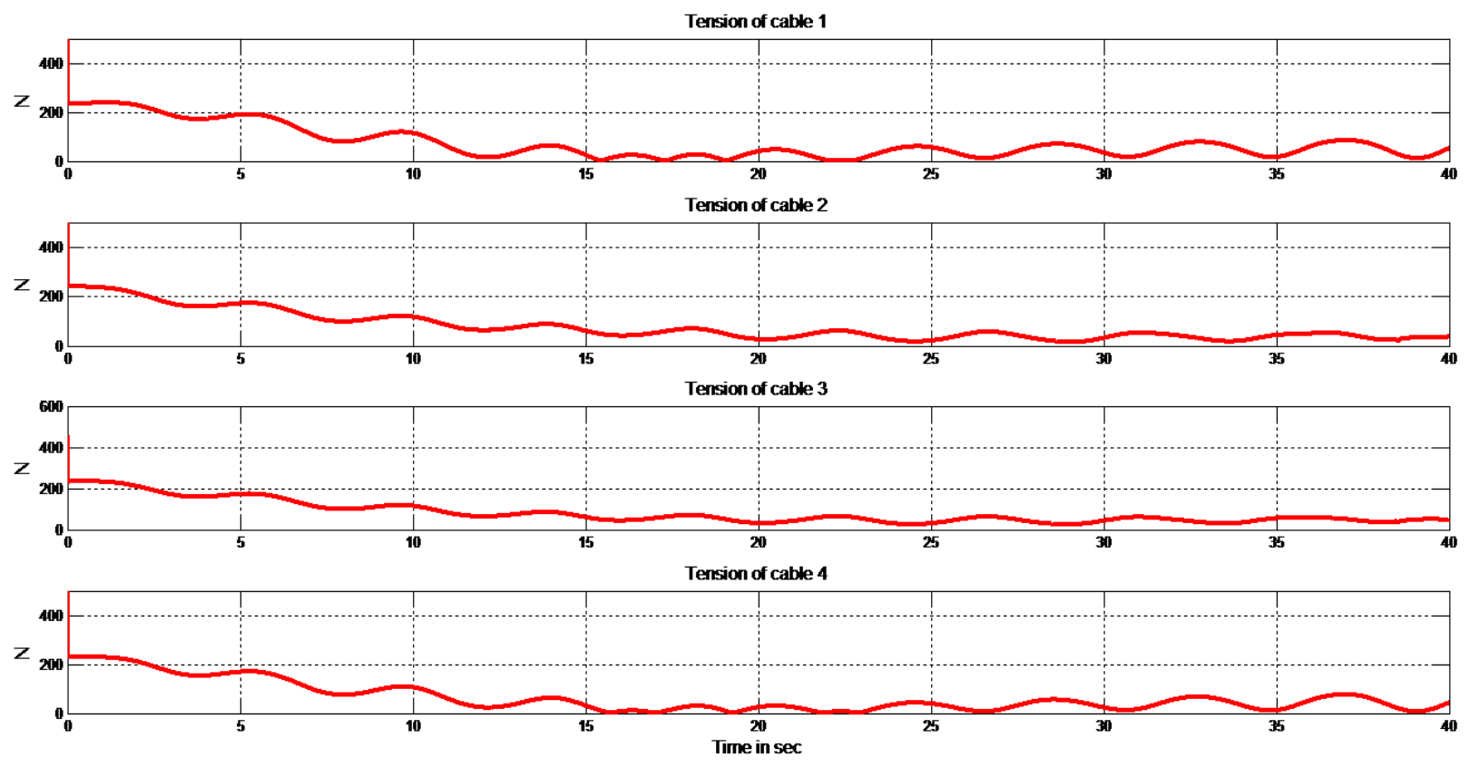
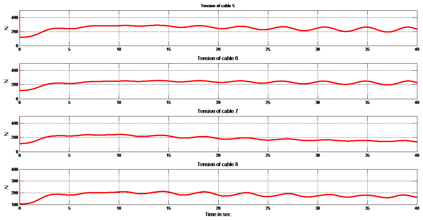
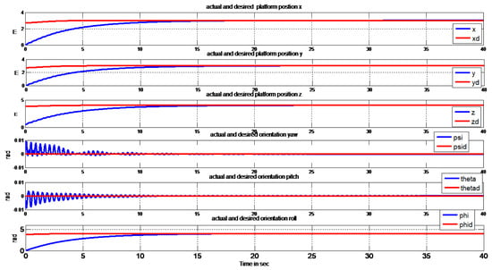
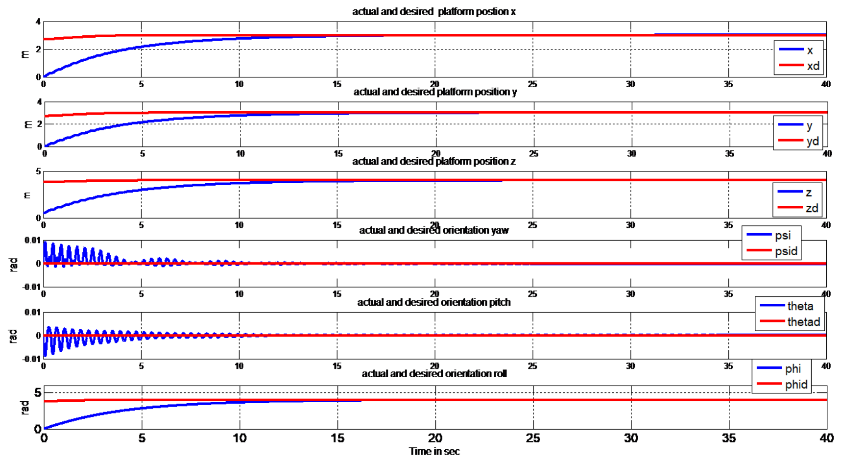
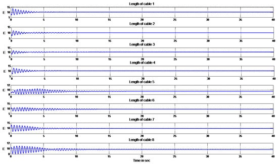
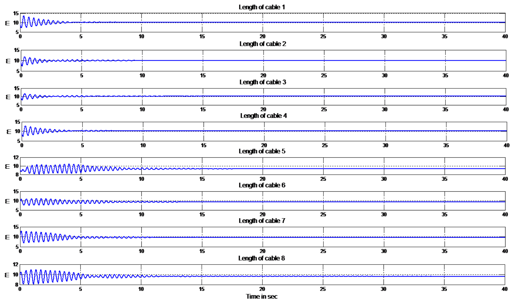
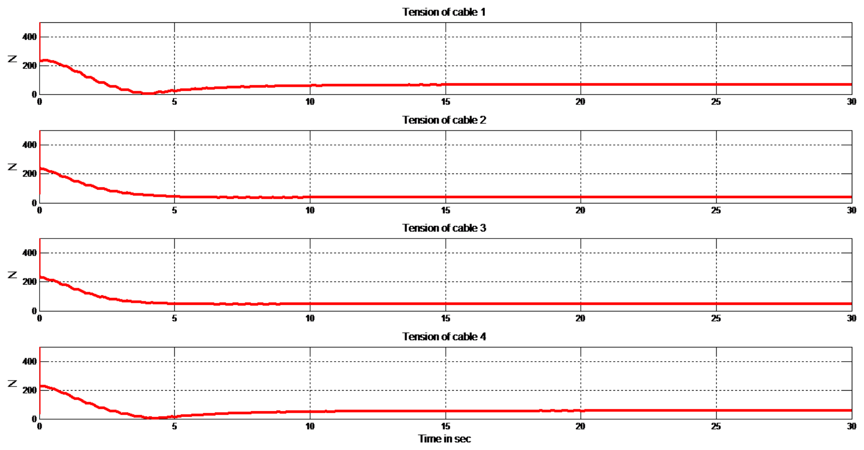
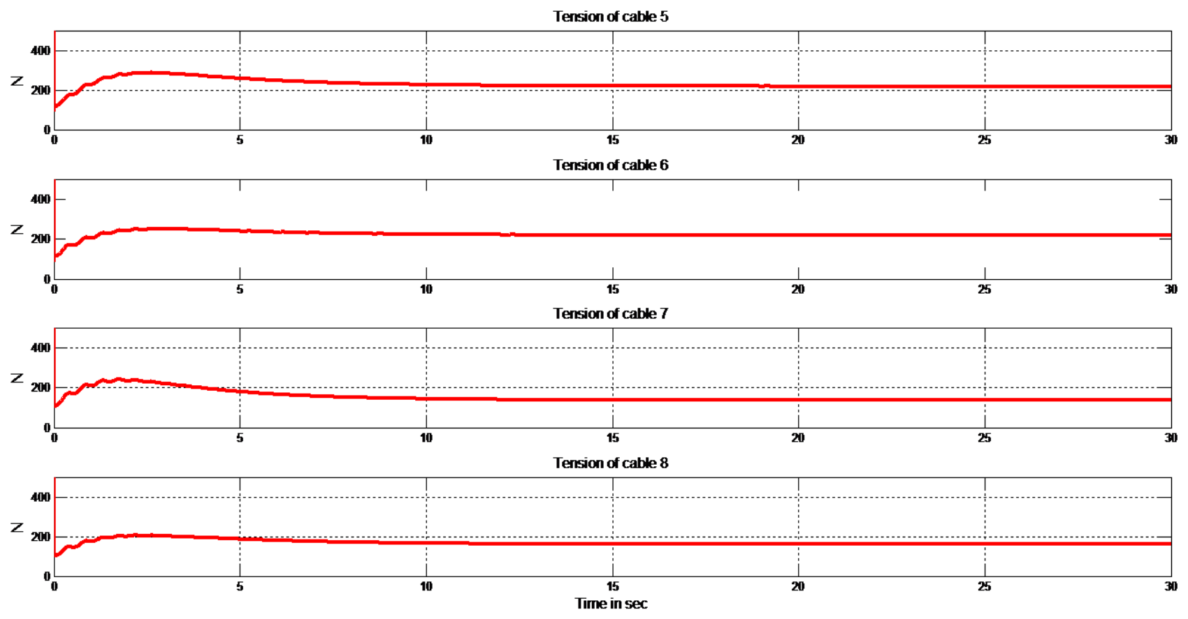
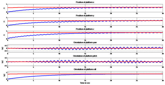
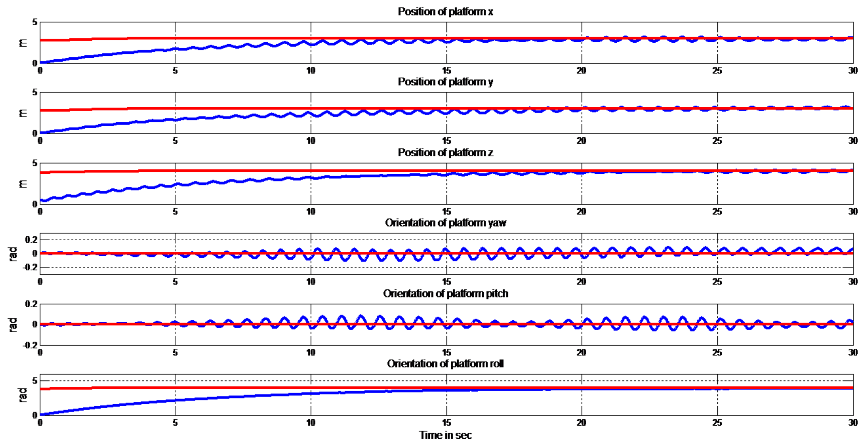
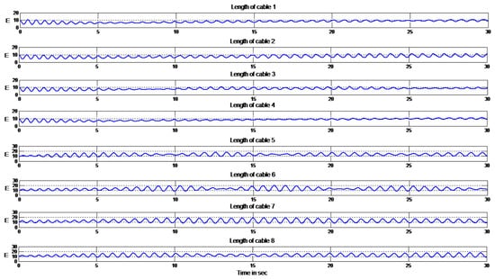
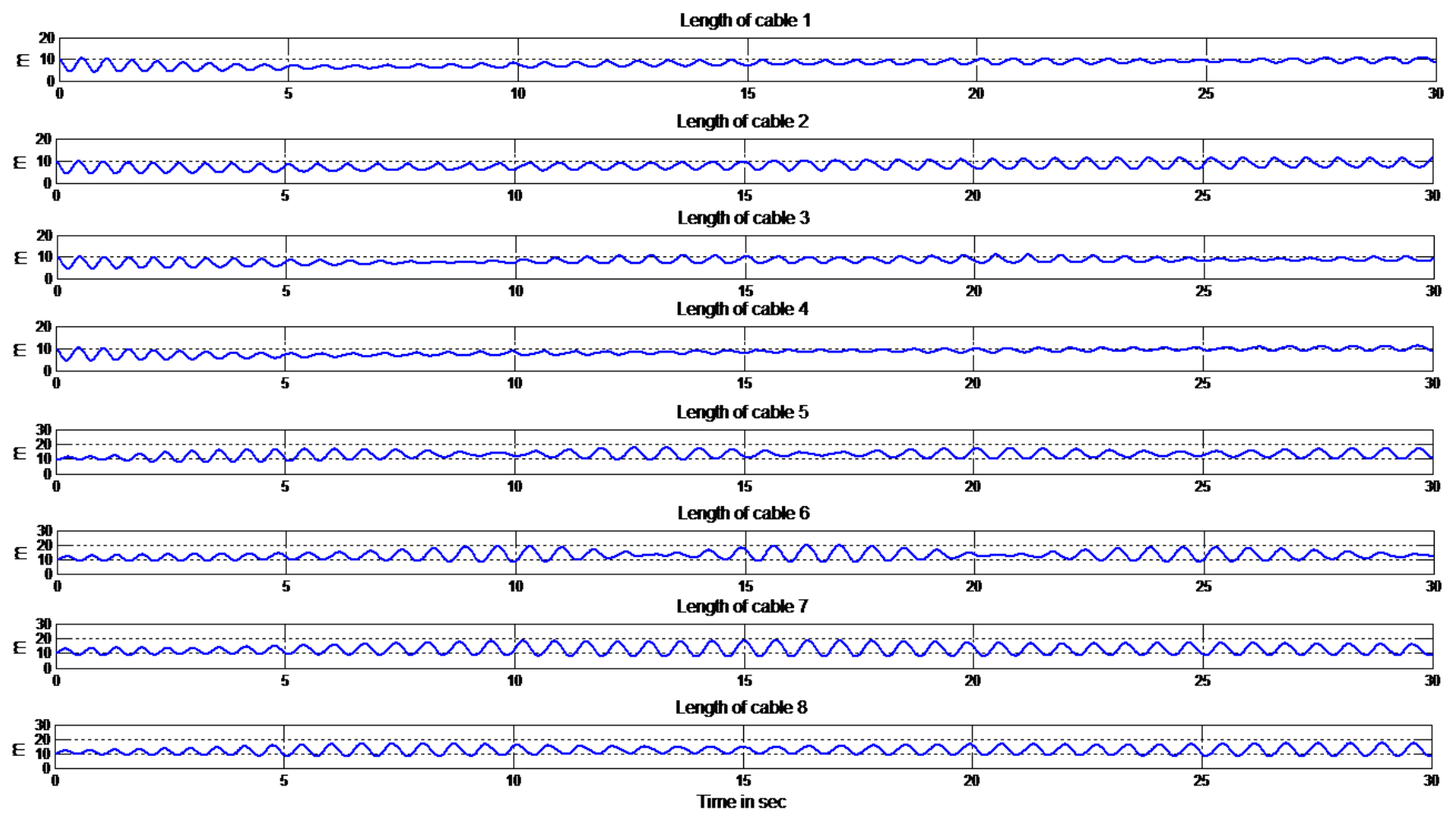
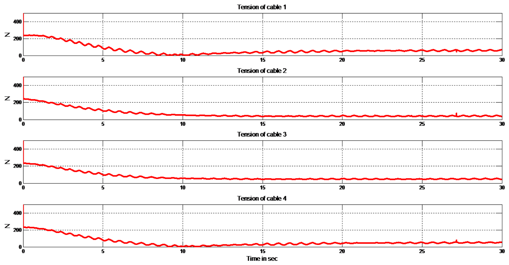
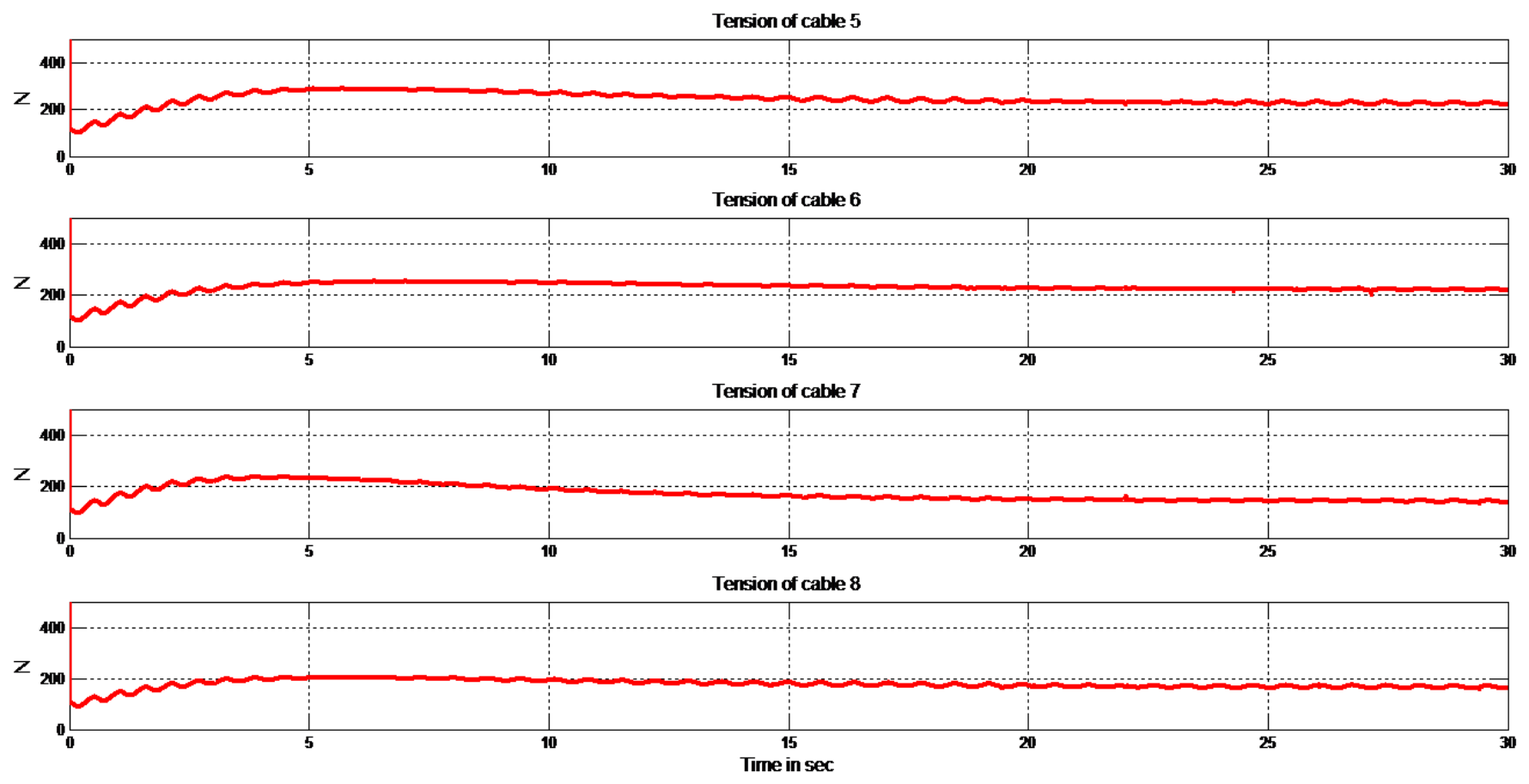
The results obtained with the baseline composite controller of [7], that is, without ADRC, are shown in Figure 3, Figure 4, Figure 5 and Figure 6. This configuration is simulated over 40 s rather than the 30 s used for the proposed controller, because its slower response requires a longer horizon to be displayed; the comparison between the two should be read over the common interval $0\le t\le 30$ s. The response is slow and oscillatory in every quantity of interest: platform position and orientation, winch coordinates and commanded cable forces. The cause is the magnitude of the gains that the baseline composite controller requires, $K_v=\mathrm{15,000}{I}_{6\times 6}$ and $K_d=\mathrm{25,500}{I}_{8\times 8}$. Such values produce an aggressive control action that induces overshoot and sustained oscillation, degrading both the stability margin and the responsiveness of the platform and yielding poor tracking. The response does not fully settle within the simulated horizon of 40 s for this configuration, which is itself an indication of how restrictive the gain selection is. The tuning of these two gains is therefore the critical constraint in the baseline composite controller, and it is precisely the constraint that the proposed controller relaxes.

Figure 3. Platform position and orientation without the ADRC scheme. Position channels in metres and orientation channels in radians against time in seconds.

Figure 4. Winch-side cable coordinate q without the ADRC scheme, in metres against time in seconds. See Notation 2.

Figure 5. Magnitude of the commanded cable force $\left|u_r\right|$ for cables 1 to 4 without the ADRC scheme, in newtons against time in seconds.

Figure 6. Magnitude of the commanded cable force $\left|u_r\right|$ for cables 5 to 8 without the ADRC scheme, in newtons against time in seconds.

4.3.2. Proposed Composite Control with ADRC

The results obtained with the proposed controller are shown in Figure 7, Figure 8, Figure 9 and Figure 10.

Figure 7. Platform position and orientation under the proposed control scheme. Position channels in metres and orientation channels in radians against time in seconds.

Figure 8. Winch-side cable coordinate q under the proposed control scheme, in metres against time in seconds. See Notation 2.

Figure 9. Magnitude of the commanded cable force $\left|u_r\right|$ for cables 1 to 4 under the proposed control scheme, in newtons against time in seconds.

Figure 10. Magnitude of the commanded cable force $\left|u_r\right|$ for cables 5 to 8 under the proposed control scheme, in newtons against time in seconds.

Figure 7 shows a response that is markedly faster and well damped, reaching the desired trajectory with high precision. The damping confirms the effectiveness of the ADRC compensation in suppressing the oscillatory behaviour observed without it. Figure 8 shows that once the transient has passed, the winch coordinates stabilise and remain constant as the platform settles at its final pose, so the compensation removes the transient elastic deformation rather than merely attenuating it. The improvement follows directly from the ability of ADRC to estimate and cancel the elastic torque in the cables, which previously produced the fluctuation and the loss of accuracy. Reducing the influence of structural compliance on the dynamic behaviour is what allows the proportional gain to be raised, and the enhanced robustness and precision are visible in both the stabilisation of the winch coordinates and the reduction of oscillation.

Figure 9 and Figure 10 show the magnitude of the commanded cable force $\left|u_r\right|$ for each of the eight cables. All eight commands settle to strictly positive, smoothly varying values with minimal oscillation, which is the condition the null-space term $\mathcal{Q}$ of (6) is chosen to enforce, since a cable can only pull. The commanded forces remain well regulated throughout, indicating effective control of the dynamic behaviour.

4.3.3. Robustness to an Added Payload

To assess the robustness of the proposed strategy, a further simulation was run with an additional payload of 35 kg attached to the platform. The results are shown in Figure 11, Figure 12, Figure 13 and Figure 14. The platform reaches and holds the commanded pose, but a residual oscillation persists on all channels for the duration of the run rather than decaying as it does in the unloaded case of Figure 7. The positioning accuracy is preserved, and the loop remains stable, so the framework tolerates a substantial change in the inertial parameters, but the damping of the fast dynamics is visibly reduced, and the gains of Table 3 would require further adjustment for the loaded configuration. This is stated rather than smoothed over, since the residual oscillation is evident in Figure 11 and Figure 12.

Figure 11. Platform position and orientation under the proposed controller with the 35 kg payload applied. Position in metres and orientation in radians against time in seconds.

Figure 12. Winch-side cable coordinate q under the proposed controller with the 35 kg payload applied, in metres against time in seconds. See Notation 2.

Figure 13. Magnitude of the commanded cable force $\left|u_r\right|$ for cables 1 to 4 under the proposed controller with the 35 kg payload applied, in newtons against time in seconds.

Figure 14. Magnitude of the commanded cable force $\left|u_r\right|$ for cables 5 to 8 under the proposed controller with the 35 kg payload applied, in newtons against time in seconds.

4.4. Quantitative Comparison

The qualitative behaviour described in Section 4.3 is quantified in Table 4. Two indices are reported. The root mean square error measures the average accuracy,

$$\mathrm{RMSE}=\sqrt{{\displaystyle \frac{1}{T-T_0}}{\int }_{T_0}^T{∥e\left(t\right)∥}^2\mathrm{d}t},$$

(39)

and the integral of time-weighted absolute error penalises errors that persist rather than decay,

$$\mathrm{ITAE}={\int }_{T_0}^{T}t∥e\left(t\right)∥\mathrm{d}t.$$

(40)

Both are evaluated over $T_0=15$ s to $T=30$ s, the interval common to all three configurations: the composite controller without ADRC is simulated for 40 s while the two ADRC configurations are simulated for 30 s (Table 2), so 30 s is the latest time at which all three records can be compared on the same axis, consistent with the common interval already identified in Section 4.3. The initial segment $0\le t<15$ s is excluded because the platform starts at $x_0={[0,0,0.5]}^{\mathsf{T}}$ m while the reference settles towards ${[3,3,4]}^{\mathsf{T}}$ m, so an index computed from $t=0$ is dominated by the initial offset of approximately $5.4$ m rather than by the tracking behaviour under comparison. The choice of $T_0$ does not drive the conclusion: repeating the computation with $T_0=10$ s and with $T_0=20$ s, keeping $T=30$ s fixed, gives position RMSE ratios between the first two configurations of $10.3$ and $6.8$ respectively, against $8.2$ for the value reported here.

Table 4. Quantitative performance of the three configurations, evaluated over $15\le t\le 30$ s, the interval common to the 40 s and 30 s runs of Table 2. Position errors are the Euclidean norm of the translational channels of $e=x_d-x$ and orientation errors that of the rotational channels.

Configuration	${\mathbf{RMSE}}_{\mathit{p}}$	${\mathbf{RMSE}}_{\mathit{o}}$	${\mathbf{ITAE}}_{\mathit{p}}$	${\mathbf{ITAE}}_{\mathit{o}}$
	[mm]	[deg]	[m·s2]	[rad·s2]
Composite control, no ADRC [7]	$1289.2$	$40.41$	$398.7$	$209.5$
Proposed, with ADRC	$157.4$	$3.45$	$51.9$	$18.1$
Proposed, with ADRC and 35 kg payload	$640.4$	$14.62$	$175.4$	$73.6$
Improvement factor, rows 1 to 2	$8.2$	$11.7$	$7.7$	$11.6$

Table 4. Quantitative performance of the three configurations, evaluated over $15\le t\le 30$ s, the interval common to the 40 s and 30 s runs of Table 2. Position errors are the Euclidean norm of the translational channels of $e=x_d-x$ and orientation errors that of the rotational channels.

Configuration	${\mathbf{RMSE}}_{\mathit{p}}$	${\mathbf{RMSE}}_{\mathit{o}}$	${\mathbf{ITAE}}_{\mathit{p}}$	${\mathbf{ITAE}}_{\mathit{o}}$
	[mm]	[deg]	[m·s2]	[rad·s2]
Composite control, no ADRC [7]	$1289.2$	$40.41$	$398.7$	$209.5$
Proposed, with ADRC	$157.4$	$3.45$	$51.9$	$18.1$
Proposed, with ADRC and 35 kg payload	$640.4$	$14.62$	$175.4$	$73.6$
Improvement factor, rows 1 to 2	$8.2$	$11.7$	$7.7$	$11.6$

Table 4 quantifies the trends visible in Figure 3, Figure 4, Figure 5, Figure 6, Figure 7, Figure 8, Figure 9, Figure 10, Figure 11, Figure 12, Figure 13 and Figure 14. The proposed controller reduces the position RMSE by a factor of $8.2$ and the orientation RMSE by a factor of $11.7$ relative to the baseline composite controller without ADRC. Over the same window the peak position error falls from 2144 mm to 299 mm, and the error at the end of the common window, $t=30$ s, falls from 1392 mm to 245 mm. The baseline value at $t=30$ s is not its final value: left to run to its own full horizon of 40 s (Table 2), the baseline error grows further, to 2149 mm, which is additional evidence, alongside Section 4.3, that the baseline configuration does not settle within the simulated horizon.

The improvement in ITAE, a factor of $7.7$ in position and $11.6$ in orientation, is of the same order as the improvement in RMSE. Because ITAE weights late error more heavily than early error, this indicates that the benefit is not confined to the transient but persists through the whole evaluation window. The result is consistent with the mechanism of Section 3: the additional gain $K_p^q$ permits a proportional gain of 3500 against 1200 for the scheme without ADRC, and it is the higher closed-loop stiffness that reduces the standing error rather than any change in the transient alone.

With the 35 kg payload the position RMSE increases from $157.4$ mm to $640.4$ mm and the position ITAE from $51.9$ to $175.4$, a degradation by factors of approximately $4.1$ and $3.4$ respectively. Within the evaluation window the position error reaches a local peak of 1768 mm near $t=20$ s, confirming that the residual oscillation visible in Figure 11 and Figure 12 is a sustained feature of this configuration rather than a decaying transient. The loaded configuration nonetheless remains better than the composite controller without ADRC, by a factor of $2.0$ in position RMSE, but the margin is markedly narrower than in the unloaded case. The gains of Table 3 were not re-optimised for the loaded case; Section 4.6 discusses what such a re-optimisation would be expected to achieve and why it is not included in the present study.

4.5. Parameter Tuning Guidelines

The controller has five tuning parameters: $K_p$ and $K_v$ for the rigid loop, ${\omega }_0$ for the extended state observer, and $K_p^q$ and $K_d$ for the fast subsystem. The stability results of Section 2.3 and Section 3 constrain these choices but do not fix them uniquely, and the following sequence was used to obtain the gains of Table 3.

Rigid loop. Lemma 1 guarantees asymptotic stability for any diagonal positive-definite $K_p$ and $K_v$, so their selection is a matter of the desired speed of response rather than of stability; $K_p$ and $K_v$ were chosen following standard second-order design practice for the rigid-body pair $(M_{eq},C_{eq})$ of (5), subject to the constraint that the resulting bandwidth remains well separated from the fast dynamics of Section 3.2, since the singular perturbation argument requires this separation.

Observer bandwidth. A larger ${\omega }_0$ tightens the residual bound of Theorem 1, but also increases the sensitivity of the estimate to any high-frequency content in the measured cable length, and, in a digital implementation, requires a correspondingly higher sampling rate; a common rule of thumb is a sampling frequency at least an order of magnitude above ${\omega }_0$. In the present, noise-free simulation study ${\omega }_0$ was set large to favour estimation accuracy, as stated in Section 3.1; Section 4.6 discusses the consequence of relaxing the noise-free assumption.

Fast-subsystem gains. $K_p^q$ sets the closed-loop stiffness that replaces the physical stiffness K in the argument following Theorem 2, and is naturally scaled by the physical stiffness range implied by $K_{sp}$ and the cable lengths of Table 1 through (3). $K_d$ must satisfy the Schur complement condition (32); too small a value leaves (32) unsatisfied and the fast subsystem underdamped, while too large a value slows the fast subsystem unnecessarily. Given a choice of $K_p^q$, (32) gives a lower bound on $K_d$ for a chosen margin $\sigma$, and $K_d$ was increased from that bound until the oscillation visible in the simulated response was acceptable.

Verification. For the selected gains, (32) and (35) were checked numerically, and the commanded cable forces of Section 4.3 were inspected to confirm they remain strictly positive over the trajectory of Section 4.2, consistent with the requirement stated in Section 2.2.

The payload configuration required a larger $K_v$ and $K_d$ than the unloaded configuration. This is because the winch inertia $a=r^{-1}{I}_m$ that enters the Schur complement condition (32) through Lemma 2 does not change with payload; the added mass enters only $m_p$ in Table 2 and, through it, the tension levels the cables must carry. Meeting (32) with adequate margin at the higher tension levels realised under the added mass called for the larger gains of Table 3. As Section 4.3 reports, the margin obtained was not sufficient to fully damp the fast dynamics under this heuristic; Section 4.6 discusses what a further increase in $K_d$ would be expected to achieve.

4.6. Limitations

The scope of the present study should be stated plainly. The validation is by simulation only; experimental confirmation on a physical cable-driven robot remains to be carried out, and effects such as pulley friction, drive-train backlash and cable hysteresis, which would all enter the total disturbance $f_q$, have not been measured. The cable model is axial, so transverse vibration, distributed cable mass and sag are not represented, and by Assumption 1, the platform is not gravitationally loaded, so the tension levels reported in Section 4.3 reflect the elastic interaction rather than the static support of the platform weight. Measurements of the cable lengths and of the platform pose are assumed noise free, which is what permits the large observer bandwidth used here; in the presence of noise, ${\omega }_0$ would have to be reduced and the estimate of $f_q$ would degrade accordingly. A static equilibrium calculation, using the geometry of Table 1 and the platform mass of Table 2, shows that the two idealisations of zero gravity and constant $K_{sp}$ are not independent. Balancing the unloaded platform weight of 294 N at the initial pose $x_0$ requires tensions of up to 553 N in the most heavily loaded cables; at $K_{sp}=900$ N, the value used throughout this study, that tension implies a static elongation of up to $6.1$ m on cables roughly 9 to 10 m long, an unrealistic strain in excess of $60\%$. Achieving a more physically reasonable strain of about $1\%$ under this load would require a specific stiffness on the order of $5.7\times {10}^4$ N, roughly sixty times the value used here. Including the full gravitational field responsibly therefore requires revisiting $K_{sp}$ together with it, rather than adding gravity to the parameter set of Table 2 unchanged; for the same reason, the tension-dependent polynomial of (4), which [14] reports for the physical cable, was not evaluated in the present study, since the force levels realised under Assumption 1 do not exercise its nonlinear regime in a way that a constant-stiffness study can usefully bound. Gravity and the tension-dependent stiffness of (4) are accordingly treated here as a linked pair of idealisations, to be addressed together, with a stiffness value re-derived for the loaded case, in future work. We stress that this is a limitation of the case study’s numerical fidelity rather than of the underlying method: as noted after Assumption 1 and after Equation (4), the control law is gravity-independent by construction and the extended state observer is agnostic to the functional form of the cable stiffness it estimates. Finally, the tension distribution relies on the null-space term $\mathcal{Q}$ of (6), whose magnitude is fixed a priori rather than optimised online against the tension limits; a closed-form force distribution such as [22] would remove that restriction and is a natural extension of the present work.

5. Conclusions

This paper has analysed the stability and control of a fully constrained cable-driven robot of large dimensions, in which the low rigidity of the cables, resulting mainly from their length, produces elastic deformation that limits both precision and bandwidth. The control framework proposed retains the composite structure of earlier work and augments it with active disturbance rejection control. It combines a rigid control component with the compensation of the elastic torque in the cables, the compensation being achieved by a damping term reinforced by an active rejection term that counteracts the elasticity-induced disturbance. Under the simulated conditions of Section 4, the advantage of the proposed controller was demonstrated by a comparison against the baseline composite controller without ADRC, reducing the root mean square position error by a factor of $8.2$ and the corresponding integral of time-weighted absolute error by a factor of $7.7$ over the evaluation window. These figures characterise the simulation study reported here and should not be read as a general engineering guarantee independent of the idealisations listed in Section 4.6.

The stability of the complete closed loop was analysed by Lyapunov’s second method and the corresponding stability conditions derived, with the extended state observer supplying the convergence property on which the boundary-layer analysis depends. Performance was then evaluated through simulation on the IPAnema3 spatial cable robot, without ADRC, with ADRC, and with ADRC under an added payload of 35 kg. The principal practical outcome is that the additional gain $K_p^q$ introduced by the compensation allows the velocity and damping gains to be reduced and the proportional gain to be increased, which is what produces the faster and more accurate platform response. Experimental validation on a physical cable-driven parallel robot, together with an online force distribution replacing the fixed null-space term, are the natural continuations of this work.

References

- Pott, A.; Mütherich, H.; Kraus, W.; Schmidt, V.; Miermeister, P.; Verl, A. IPAnema: A family of cable-driven parallel robots for industrial applications. In Cable-Driven Parallel Robots; Mechanisms and Machine Science; Springer: Berlin/Heidelberg, Germany, 2013; Volume 12, pp. 119–134. [Google Scholar] [CrossRef] [Scilit]
- Kawamura, S.; Choe, W.; Tanaka, S.; Pandian, S.R. Development of an ultrahigh speed robot FALCON using wire drive system. In Proceedings of the 1995 IEEE International Conference on Robotics and Automation, Nagoya, Japan, 21–27 May 1995; pp. 215–220. [Google Scholar] [CrossRef] [Scilit]
- Izard, J.-B.; Dubor, A.; Hervé, P.-E.; Cabay, E.; Culla, D.; Rodriguez, M.; Barrado, M. Large-scale 3D printing with cable-driven parallel robots. Constr. Robot. 2017, 1, 69–76. [Google Scholar] [CrossRef] [Scilit]
- Merlet, J.-P.; Daney, D. A portable, modular parallel wire crane for rescue operations. In Proceedings of the 2010 IEEE International Conference on Robotics and Automation, Anchorage, AK, USA, 3–7 May 2010; pp. 2834–2839. [Google Scholar]
- Gouttefarde, M.; Rodriguez, M.; Barrelet, C.; Hervé, P.-E.; Creuze, V.; Gorrotxategi, J.; Oyarzabal, A.; Culla, D.; Sallé, D.; Tempier, O.; et al. The robotic seabed cleaning platform: An underwater cable-driven parallel robot for marine litter removal. In Cable-Driven Parallel Robots (CableCon 2023); Mechanisms and Machine Science; Springer: Cham, Switzerland, 2023; Volume 132, pp. 430–441. [Google Scholar] [CrossRef] [Scilit]
- Qian, S.; Zi, B.; Shang, W.-W.; Xu, Q.-S. A review on cable-driven parallel robots. Chin. J. Mech. Eng. 2018, 31, 66. [Google Scholar] [CrossRef] [Scilit]
- Khosravi, M.A.; Taghirad, H.D. Dynamic modeling and control of parallel robots with elastic cables: Singular perturbation approach. IEEE Trans. Robot. 2014, 30, 694–704. [Google Scholar] [CrossRef] [Scilit]
- Ottaviano, E.; Castelli, G. A study on the effects of cable mass and elasticity in cable-based parallel manipulators. In ROMANSY 18 Robot Design, Dynamics and Control; CISM International Centre for Mechanical Sciences; Springer: Vienna, Austria, 2010; Volume 524, pp. 149–156. [Google Scholar] [CrossRef] [Scilit]
- Meunier, G.; Boulet, B.; Nahon, M. Control of an overactuated cable-driven parallel mechanism for a radio telescope application. IEEE Trans. Control Syst. Technol. 2009, 17, 1043–1054. [Google Scholar] [CrossRef] [Scilit]
- Khosravi, M.A.; Taghirad, H.D. Dynamic analysis and control of cable-driven robots with elastic cables. Trans. Can. Soc. Mech. Eng. 2011, 35, 543–557. [Google Scholar] [CrossRef] [Scilit]
- Taghirad, H.D.; Khosravi, M.A. Stability analysis and robust composite controller synthesis for flexible joint robots. Adv. Robot. 2006, 20, 181–211. [Google Scholar] [CrossRef] [Scilit][Green Version]
- Vafaei, A.; Khosravi, M.A.; Taghirad, H.D. Modeling and control of cable driven parallel manipulators with elastic cables: Singular perturbation theory. In Intelligent Robotics and Applications (ICIRA 2011); Lecture Notes in Computer Science; Springer: Berlin/Heidelberg, Germany, 2011; Volume 7101, pp. 455–464. [Google Scholar] [CrossRef] [Scilit]
- Kokotović, P.; Khalil, H.K.; O’Reilly, J. Singular Perturbation Methods in Control: Analysis and Design; Academic Press: London, UK, 1986. [Google Scholar]
- Kraus, W. Force Control of Cable-Driven Parallel Robots. Ph.D. Thesis, University of Stuttgart, Stuttgart, Germany, 2015. [Google Scholar] [CrossRef]
- Han, J. From PID to active disturbance rejection control. IEEE Trans. Ind. Electron. 2009, 56, 900–906. [Google Scholar] [CrossRef] [Scilit]
- Huang, Y.; Xue, W. Active disturbance rejection control: Methodology and theoretical analysis. ISA Trans. 2014, 53, 963–976. [Google Scholar] [CrossRef] [Scilit] [PubMed]
- Zheng, Q.; Gao, Z. Active disturbance rejection control: Between the formulation in time and the understanding in frequency. Control Theory Technol. 2016, 14, 250–259. [Google Scholar] [CrossRef] [Scilit]
- Feng, H.; Guo, B.-Z. Active disturbance rejection control: Old and new results. Annu. Rev. Control 2017, 44, 238–248. [Google Scholar] [CrossRef] [Scilit]
- Fareh, R.; Al-Shabi, M.; Bettayeb, M.; Ghommam, J. Robust active disturbance rejection control for flexible link manipulator. Robotica 2020, 38, 118–135. [Google Scholar] [CrossRef] [Scilit]
- Cuvillon, L.; Weber, X.; Gangloff, J. Modal control for active vibration damping of cable-driven parallel robots. J. Mech. Robot. 2020, 12, 051004. [Google Scholar] [CrossRef] [Scilit]
- Saadaoui, R.; Piccin, O.; Bara, G.I.; Laroche, É. Modeling and control of a three degrees-of-freedom planar cable-driven parallel robot with flexible cables. J. Dyn. Syst. Meas. Control 2025, 147, 051009. [Google Scholar] [CrossRef] [Scilit]
- Pott, A.; Bruckmann, T.; Mikelsons, L. Closed-form force distribution for parallel wire robots. In Computational Kinematics; Springer: Berlin/Heidelberg, Germany, 2009; pp. 25–34. [Google Scholar] [CrossRef] [Scilit]
Disclaimer/Publisher’s Note: The statements, opinions and data contained in all publications are solely those of the individual author(s) and contributor(s) and not of MDPI and/or the editor(s). MDPI and/or the editor(s) disclaim responsibility for any injury to people or property resulting from any ideas, methods, instructions or products referred to in the content. |
© 2026 by the authors. Licensee MDPI, Basel, Switzerland. This article is an open access article distributed under the terms and conditions of the Creative Commons Attribution (CC BY) license.