


Abstract
Mediterranean Dehesa woodlands require monitoring of tree structural change, but conventional stem-diameter inventories are labor-intensive. Mobile simultaneous localization and mapping (SLAM) LiDAR can acquire three-dimensional tree structure, although inconsistent trajectories and uneven stem coverage may reduce measurement repeatability. This study evaluated whether a teleoperated quadruped carrying a Hovermap ST sensor along standardized circular trajectories could acquire stem-level point clouds suitable for diameter-at-breast-height (DBH) estimation in open Dehesa terrain. Backpack-mounted surveys were conducted in 2025 at Majadas de Tiétar, followed by quadruped-mounted surveys in 2026 at two Spanish sites. DBH was derived from horizontal slices at 1.3 m using Circle Fitting, Convex Hull Peeling, and Kalman-filter reconstruction, then compared with height-matched manual references. Backpack estimates for 186 caliper-referenced observations achieved R2 values of 0.853–0.869, Lin’s concordance coefficients of 0.787–0.833, and root-mean-square errors of 5.22–6.11 cm. After excluding one bifurcation-affected observation, 29 robot estimates achieved R2 values of 0.930–0.943, concordance coefficients of 0.941–0.956, and root-mean-square errors of 3.17–3.84 cm. Robot acquisitions showed more balanced radial point distributions and fewer reconstruction errors. However, dataset differences preclude controlled platform comparison. Quadruped-mounted SLAM LiDAR therefore shows promise for standardized one-time DBH inventories, while paired same-tree repeatability studies remain necessary before application to multitemporal growth monitoring.
1. Introduction
The Mediterranean savanna-like woodlands in the southwest of the Iberian Peninsula, known as Dehesa in Spain and Montado in Portugal, represent one of the 25 biodiversity hotspots in Europe and its largest silvo-pastoral system [1,2]. They are outstanding examples of environmental and socioeconomic importance and therefore have particularly high conservation value [3]. In this system, trees are keystone elements because they provide ecosystem services that exceed the area they occupy [4]. However, this silvo-pastoral ecosystem, composed primarily of evergreen oak trees, is threatened by oak decline events that have occurred increasingly since the early 1980s. These episodes of decline are primarily driven by complex interactions between abiotic factors such as drought, nutrient limitation, and water availability, and the biotic soil-borne pathogen Phytophthora cinnamomi [5].
To detect and mitigate tree decline, monitoring tree vitality is crucial. Structural traits derived from repeated measurements provide useful indicators of vitality because they capture changes in tree form, growth, and crown condition over time. Under stressors such as drought, disease, or defoliation, canopy-level photosynthetic capacity can decline as leaf area or leaf function is impaired; at the same time, remaining foliage may partly compensate, and carbon allocation may shift among maintenance, defense, storage, repair, and growth [6,7]. Accordingly, temporal changes in structural metrics can provide context-sensitive indicators of vitality, especially when interpreted alongside physiological and environmental information. Relevant metrics include stem growth, crown extent, crown density, and other geometric descriptors of tree architecture.
To measure those metrics, there are well-established methods. Stem diameter is commonly measured with diameter tapes or calipers, tree height with clinometers or hypsometers, and crown dimensions with tape-based or optical measurements. Stand-level attributes such as tree density and basal area are derived from plot inventories, sometimes supported by angle-count methods using prisms or relascopes. Tree condition can additionally be assessed visually through characteristics such as crown density, defoliation, stem damage, or mortality. These methods are inexpensive and robust, but they are labor intensive and provide only a limited representation of three-dimensional tree structure [8].
Remote and proximal sensing technologies allow tree structure to be assessed across spatial scales using different sensors and platforms [9]. Three-dimensional point clouds from light detection and ranging (LiDAR) are especially useful because laser pulses can sample stems, branches, and crowns without destructive field sampling [10,11]. Airborne laser scanning (ALS) and terrestrial laser scanning (TLS) have already been used to measure structural traits in Dehesa ecosystems. For example, Bogdanovich et al. [12] derived diameter at breast height (DBH), tree height, and crown area from TLS, and García et al. [13] used TLS and ALS to assess canopy clumping. While highly accurate, static TLS remains time-consuming because several scan positions must be co-registered to reduce occlusion. In contrast, ALS can scan large areas in a single survey, but it provides lower point density near stems and in the lower crown [10,14].
Portable simultaneous localization and mapping (SLAM) LiDAR can reduce some of these limitations. Handheld, backpack-mounted, and robot-mounted SLAM systems map their surroundings while estimating sensor poses during movement [15]. Backpack and handheld SLAM LiDAR have achieved DBH accuracies close to static TLS in several forest settings [16,17,18]. However, SLAM point-cloud quality can still be affected by motion distortion, pose drift, incomplete stem coverage, and uneven point density. These limitations are especially relevant for repeated monitoring, because changes in walking path, sensor orientation, and scan angle can create spatial mismatches between survey dates [19]. In addition, these scan inconsistencies can bias derived tree structure metrics, highlighting the need for more standardized acquisition trajectories [20].
Robotic platforms offer a potential advantage over human-carried systems because they can facilitate more standardized acquisition conditions, including movement speed, sensor geometry, and scanning trajectory. The principal motivation for using a robotic platform is therefore not necessarily to achieve higher point-cloud quality during an individual survey, as human-carried SLAM systems can also provide accurate tree measurements. Rather, robotic platforms may reduce operator-dependent variation between repeated acquisitions. This is particularly relevant for multitemporal monitoring, where small structural changes must be distinguished from differences introduced by the acquisition procedure itself.
Previous robot-mounted SLAM LiDAR studies for tree monitoring have primarily focused on autonomous navigation, in which robots follow waypoints while determining their exact trajectories from onboard perception and local mapping [15,21,22,23]. Although such approaches enable autonomous operation, autonomy does not necessarily guarantee that identical sensor trajectories are reproduced between trees or survey dates. For monitoring applications, the ability to execute a predefined spatial trajectory repeatedly may therefore provide an additional advantage. GNSS/RTK-based navigation has already been demonstrated for robotic platforms [24], indicating that externally referenced navigation along predefined paths is technically feasible. Such an approach could potentially be used to reproduce standardized LiDAR acquisition trajectories across repeated surveys.
The relevance of this is even greater in open savannah-like landscapes such as Dehesa wood-pastures, where tree density is low. On the one hand, these landscapes provide fewer geometric features for SLAM registration than typical forest stands; on the other hand, they allow standardized trajectories through which individual trees can be observed separately from all sides. Furthermore, these landscapes are often characterized by rough, sloping terrain and seasonal grass growth that can reach the height of a quadruped robot. Such vegetation can act as a physical obstacle, making autonomous navigation more difficult and potentially causing robot malfunctions.
To our knowledge, quadruped-mounted SLAM LiDAR has not yet been evaluated for diameter-grade stem reconstruction under these conditions. Radial stem growth is one of the most practical structural indicators because it integrates cumulative growth responses over time and can be measured repeatedly as DBH. Compared with crown-based metrics, DBH is less affected by short-term variability, such as wind-induced crown motion and is relatively easy to validate against manual measurements. For this reason, DBH provides a robust first test metric for evaluating whether a robot-based scanning workflow can generate geometrically reliable tree measurements before extending the approach to more complex vitality-related traits.
For these reasons, we developed a workflow in which a teleoperated quadruped robot followed a preplanned circular trajectory around individual holm oak trees. The planned path was marked using chalk circles to experimentally impose a standardized trajectory. These markings were not intended to represent a final operational workflow, but rather to provide a controlled field approximation of a trajectory that could later be supplied digitally to a robot through an appropriate positioning and navigation system. By combining a predefined trajectory with approximately constant movement speed, the experiment aimed to control important platform-related components of the scanning procedure.
Unlike autonomous waypoint-based navigation, this approach enforces a consistent path around each tree, which should reduce occlusion, and provide more standardized stem coverage for diameter estimation and future growth monitoring.
We evaluated whether a teleoperated quadruped carrying a SLAM LiDAR sensor can acquire stem-level point clouds suitable for tree stem diameter estimation in savanna-like or silvo-pastoral ecosystems. We also investigated whether standardized scanning patterns produced more even point distributions and whether point distribution affected trunk reconstruction. Because the robot- and backpack-based datasets were acquired under different sampling and reference conditions, their comparison is intended to characterize workflow-specific patterns rather than to establish a controlled causal advantage of the robotic platform over human-carried SLAM acquisition. The study addressed the following questions:
- 1.
- Can the teleoperated quadruped-mounted SLAM system complete standardized circular scan paths around individual trees under open Dehesa terrain conditions?
- 2.
- How accurately do diameter estimates derived from SLAM stem slices using Circle Fitting, Convex Hull Peeling, and Kalman-filter reconstruction agree with manual reference measurements?
- 3.
- How do errors differ between robot-mounted SLAM workflows with standardized scanning patterns and backpack-mounted SLAM workflows with non-standardized scanning patterns when differences in the reference method and sampling design are made explicit?
- 4.
- Are the scanning approach- and reference-specific error magnitudes small enough to support one-time diameter inventory measurements?
- 5.
- How does the point distribution within segmented stem slices differ between standardized robot-based and non-standardized backpack-based scanning patterns?
- 6.
- How is slice point distribution associated with trunk-reconstruction quality?
2. Materials and Methods
2.1. Study Sites
The study was conducted at two sites within the Dehesa landscape, the silvo-pastoral land-use system of the southwestern Iberian Peninsula (Figure 1).Dehesas are characterized by an open tree layer, commonly dominated by evergreen oaks such as holm oak (Quercus ilex) and cork oak (Quercus suber), combined with livestock grazing and, in some areas, crop production [25]. The same silvo-pastoral land-use system extends into southern Portugal, where it is known as montado [26]. Their open canopy structure and long management history distinguish them from closed-canopy forests and make them a relevant test case for SLAM-based mobile laser scanning. The tree layers of Dehesa and montado systems are dominated by mature trees, commonly showing past injuries from former pruning or other legacy events [27,28].
Figure 1.
Overview of the study areas and scanned-tree areas used for the SLAM LiDAR surveys. The top row shows the Majadas site in Extremadura, Spain, with separate backpack-mounted and robot-mounted scan areas, while the bottom-left panel shows the robot-mounted scan area at the San Francisco site in Andalusia, Spain. Red polygons delineate the scanned-tree areas. The bottom-right overview map shows the locations of both study sites on the Iberian Peninsula, marked by numbered red stars: (1) Majadas and (2) San Francisco. Dashed outlines represent Spanish province boundaries, and solid outlines represent country borders. Site coordinates are provided in the panel headers.
The first site is located near Majadas de Tiétar (short: MAJ) in the province of Cáceres, Extremadura, Spain. The site is a managed Dehesa with open evergreen holm oak cover and gently undulating terrain. The second site is located at Dehesa San Francisco (short: SF) in the province of Huelva, Andalusia, Spain, in the foothills of the Sierra Morena. Compared with MAJ, SF includes more rugged terrain and a more heterogeneous vegetation cover, which was used to evaluate robot traversability under less favorable field conditions (Table 1).
Table 1.
Study-site characteristics and sampling design for the two Spanish Dehesa field sites used for SLAM LiDAR acquisition and manual diameter validation. The table summarizes geographic location, area of interest, elevation and terrain context, dominant tree species, platform-specific data acquisition, and available reference measurements.
2.2. SLAM LiDAR Measurements
2.2.1. Technical Description
The SLAM LiDAR sensor used for the survey was the Hovermap ST (Emesent, Brisbane, QLD, Australia), which weighs approximately . The scanner has a range of 0.4 m to 100 m, an outdoor accuracy of , and a field of view of . In single-return mode, the sensor captures 300,000 points s−1, while in the dual-return mode 600,000 points/s are captured. The sensor uses the Wildcat SLAM algorithm, which combines an odometry module and pose-graph optimization [29]. The SLAM algorithm was not modified in this study. Manufacturer-reported mapping and positioning accuracy metrics were used as system specifications, while study-specific reconstruction accuracy was assessed separately from surveyed checkpoints. The same sensor was mounted on a backpack frame or on a quadruped robot.
2.2.2. Backpack-Mounted Platform
The backpack configuration used the Hovermap ST sensor mounted on a rigid backpack frame approximately above ground (Figure 2a), running in dual-return mode. The sensor orientation was vertical to the ground, and the operator walked with an approximate speed of 1.5 m·s−1.
Figure 2.
SLAM LiDAR acquisition setups used in the study: (a) backpack-mounted Hovermap ST carried by a human operator and (b) Hovermap ST mounted on the Unitree Go2 Pro quadruped. The robot was remote-controlled during the field campaign.
2.2.3. Quadruped-Mounted Platform
The quadruped platform was a Unitree Go2 Pro (Unitree Robotics, Hangzhou, Zhejiang, China) carrying the Hovermap ST on a rigid mid-back mount (Figure 2b). The total payload, including scanner, mounting plate, rail system, cabling, and protective housing, was approximately . The scanner origin was mounted approximately above the ground, in front of the center of the robot body, and above the robot mounting plate. The sensor was also operated in dual-return mode. During data acquisition, the robot was remote-controlled at an approximate walking speed of 1.5 m·s−1.
2.3. Georeferencing
For georeferencing, five ground control points with a radius of were deployed in each scan. Marker positions were measured using either one of the two Base/Rover DGPS RTK positioning systems: (1) a Topcon GR-5 (Topcon Positioning Systems, Livermore, CA, USA; relative accuracy 10 + 1 ppm horizontal and 15 + 1 ppm vertical, Figure 3a) or (2) an Emlid Reach RS4 Pro (Emlid, Budapest, Hungary; relative accuracy 7 + 1 ppm horizontal and 14 + 1 ppm vertical, Figure 3b). The absolute location of the base stations was determined with an EOS Skadi Gold GNSS receiver (Eos Positioning Systems, Terrebonne, QC, Canada) together with the “Red Extremeña de Posicionamiento” correction service, providing a horizontal accuracy of <1 cm and a vertical accuracy of <2 cm. In addition, across the scans used for analysis, a total of 10 ground control points were used as checkpoints for accuracy evaluation instead of georeferencing. These checkpoint errors were used as a map-quality diagnostic and were not interpreted as a direct measure of SLAM trajectory error because they may contain contributions from sensor ranging, SLAM reconstruction, GNSS reference measurements, and the subsequent georeferencing transformation.
Figure 3.
(a) Measuring a ground control point with the Topcon GR-5 rover. (b) Emlid Reach RS4 Pro in base station mode.
2.4. Field Acquisition Design
Data were gathered during two field campaigns. The first campaign was conducted between 20 June 2025 and 4 July 2025 in MAJ. In total, 11 scans were acquired using the backpack system. Each of the 266 trees in the AOI (Figure 1) was looped at least twice. One loop was walked directly below the crown around the stem and one larger loop was walked around the perimeter of the crown. The loops did not follow a planned pattern; instead, the operator freely attempted to walk in a circular path around the trees. Eighteen trees were scanned two or three times because of overlaps between scans, resulting in 284 tree instances assessed in the point clouds. The second field campaign was conducted between 9 May 2026 and 16 May 2026. Twenty trees were scanned at MAJ, and ten trees were scanned at SF using the quadruped-mounted system. Around each tree, chalk circles with a radius of were marked around the stem. The chalk circles were used as visual guidance for the remote operator and as a field approximation of a repeatable, standardized trajectory. The scans, therefore, evaluate controlled teleoperation rather than autonomous path following. During the scans, each tree was looped twice by following the outer border of the chalk circles (Figure 4).
Figure 4.
(a) Chalk-circle guidance used for controlled teleoperated robot scanning around individual trees. The target circle radius was 1.5 m. (b) Unitree Go2 Pro carrying the Hovermap ST during a chalk-guided scan.
2.5. Manual Reference Measurements
Manual field measurements were used as reference data to evaluate LiDAR-derived diameter estimates. We avoid the term validation because the reference instruments differ in their measurement principles and are themselves subject to measurement error. Manual measurements were obtained using either a caliper to measure a directional stem diameter at 1.30 m, a diameter tape to derive a circumference-equivalent diameter at the respective measurement height, or dendrometers installed at heights selected for growth monitoring. For non-circular stems, such as the studied oaks, which can deviate substantially from circularity [12], these measurement principles are not fully interchangeable. Therefore, agreement metrics were interpreted separately for each reference dataset and were not used to directly rank reference instruments or carrier platforms.
The diameter at breast height (DBH) was used as the primary reference variable, as it is the dominant convention to express the size of the stem in forest inventories and to link the diameter of the stem with growth, biomass, and allometric analyses [8,30,31]. Although DBH is commonly treated as a standardized field quantity, the actual measurement height has varied among measurement traditions; common conventions are approximately and, in the United States, (4.5 ft) above ground [30,32]. The DBH measurement height should therefore be understood primarily as an operational and historical standard, rather than as a biologically unique point on the stem. In particular, the U.S. 4.5 ft convention has been traced to Pinchot’s 1899 description of this height as customary [33] p. 48; see also Magarik [32].
Three reference datasets were used to calculate the diameter-agreement metrics described in Section 2.8. The first data set includes reference dendrometer observations from the 2025 backpack campaign in MAJ. The dendrometers were installed slightly above or below , and the measurement height for each tree was chosen at the minimum diameter of the local stem to prioritize the monitoring of growth increases, avoiding lower branches and eventual stem deformations. Therefore, these values were treated as diameter references at the height of the dendrometer installation rather than as strict DBH references when the height of the installation differed from .
The second dataset consists of reference caliper observations measured at in September 2024 in MAJ and matched to valid stem slices derived from the 2025 backpack SLAM LiDAR campaign. These observations were treated as DBH references.
The third dataset was collected during the 2026 robot campaign using a diameter tape. All 30 robot-scanned trees were measured at , , and , providing 90 height-specific reference observations before exclusion of the non-comparable treeID23 breast-height observation. Measurement height was referenced to the highest ground point at the base of each trunk. Measurements at are reported as diameter at breast height (DBH), whereas measurements at and are reported as diameter at measurement height (DMH) and are not interpreted as DBH. For the robot-mounted scans, LiDAR-derived diameters were evaluated at the height of the corresponding manual reference measurement. Because each tree contributed observations at three heights, measurements from different heights on the same tree were treated as repeated observations and were not pooled in the reported ordinary least-squares agreement analyses.
In the oak stands studied, a canonical measurement of DBH at was not always feasible or unambiguous because several trees forked, leaned, or developed an irregular stem geometry below or near the height of the breast. For trees that fork below breast height, a measurement at may no longer represent a single approximately cylindrical stem section and may instead intersect a fork, swelling, or multiple stems. Similar difficulties have been described for multi-stemmed and forked trees, for which lower-height measurements, such as diameter at 30 () or measurements immediately below the fork, can improve repeatability and operational consistency [34,35]; more generally, lower-stem diameters have also been evaluated as alternatives or conversion points when measurements at are not possible [31,36]. Therefore, for the robot–diameter-tape dataset, we evaluated stem diameter at three fixed heights (, , and ), using height-matched tape measurements as reference values. These measurements are interpreted as the diameter at the measurement height, rather than as interchangeable DBH values; this follows the recommendation to explicitly state the actual measurement height when the term DBH is ambiguous [30]. The height-split analysis should, therefore, be interpreted as a sensitivity analysis of measurement height and method performance, with the caveat that some observations remain partly confounded by tree form, fork position, local stem irregularity, and the feasibility of obtaining a valid tape reference at the same height.
2.6. Data Analysis
The data analysis comprised several successive processing and analytical steps, from the pre-processing and georeferencing of the raw point-cloud data to the extraction and evaluation of the relevant metrics. An overview of the complete data analysis workflow is provided in Figure 5, while the individual steps are described in detail in the following sections.
Figure 5.
Five-stage processing workflow for the dataset-specific agreement assessment of SLAM LiDAR-derived stem diameters. The Hovermap ST was carried either by a backpack operator or by a human-teleoperated Unitree Go2 Pro guided around visually marked chalk circles. The two branches represent different field campaigns and differ in trajectory protocol, processing settings, height normalization, tree segmentation or stem isolation, slice definition, and manual reference instrument. The workflow, therefore, does not represent a controlled comparison of carrier platforms. The backpack–caliper analysis and the robot m analysis concern diameter at breast height (DBH); robot measurements at and m concern diameter at measurement height (DMH). The backpack–dendrometer comparison relates m LiDAR slices to dendrometer references recorded at installation heights near, but not necessarily equal to, m. Agreement and quality metrics are interpreted within each dataset. Detailed processing parameters are reported in the Methods section.
2.6.1. Pre-Processing
The raw Hovermap scans were processed in the Aura software (Emesent, Brisbane, Australia, version 2.1.1). Each scan was processed separately using the following settings: moving-object filtering = enabled, adaptive statistical outlier removal = enabled (NN = 50; = 0.1), denoise statistical outlier removal = enabled (NN = 50; log scale = 6), surface-noise reduction = enabled (low for backpack, high for robot), and output point format = LAZ 1.4. Scans were georeferenced using five ground control points distributed across each AOI and measured with either the GR-5 base/rover constellation (backpack scans) or the Emlid base/ rover constellation (quadruped robot scans).
2.6.2. Automated Tree Segmentation and Stem Isolation of Backpack-System-Derived Point Clouds
Further processing of the backpack scans was conducted using an R (version 4.5.2) script based on the lidR package. First, each scan was clipped to its respective AOI so that only trees that had been looped twice during the corresponding scan were retained. A range filter was then applied to remove all points with a range value ≥20 m, as measurement accuracy decreases with increasing scanner-to-target distance.
The filtered point clouds were subsequently classified into ground and non-ground points using a progressive morphological filter [37]. The window size was set to 1 , and the height threshold above ground was set to . Heights were then normalized to height above ground using spatial interpolation based on inverse-distance-weighted k-nearest-neighbor interpolation [38]. The number of neighbors was set to 10 and the power factor to 2. All subsequent height-dependent processing steps, including the extraction of points at breast height, were based on these normalized heights.
A stem-marker segmentation workflow was then developed to segment individual trees from the backpack-system point clouds. The workflow was adapted from the code provided by Irwin et al. [39]. In broad-leaved evergreen trees such as holm oak, crown radius and crown height can vary substantially among individuals and within individual crowns [40]. This variability can lead to over-segmentation when a local-maximum filter is applied directly to the canopy surface. Therefore, stem markers rather than canopy maxima were used as seed points for the watershed segmentation.
The workflow consisted of five main steps: isolating potential stem points, detecting stem markers using local-maximum filtering, increasing marker heights, modifying the canopy height model (CHM) around the markers, and deriving crown polygons using a watershed algorithm. First, the normalized point cloud was clipped at a height of above ground to retain points around breast height. For each remaining point, the number of neighboring points within a radius of was calculated, and points with 200 or fewer neighbors were removed. This neighborhood-density filter was applied to remove sparse noise and returns from tall grass or other understory vegetation that could otherwise be falsely identified as tree stems. The appropriate number-of-neighbors threshold depends strongly on the characteristics of the point cloud, which are influenced by the scanner used, the scanning approach, scanning duration, and resulting point density. Consequently, this parameter must be selected manually for the specific acquisition scenario rather than being treated as a universally applicable value.
Two CHMs were subsequently generated: one from the point cloud clipped at , with a spatial resolution of , and one from the complete normalized point cloud, with a spatial resolution of . A local-maximum filter with a window size of 11 and a minimum height of 1 was applied to the CHM derived from the clipped point cloud to identify stem markers (Figure 6a). The marker heights were then increased by 11 . The magnitude of this increase should be selected such that the resulting marker height is at least equal to the height of the tallest tree within the AOI, thereby ensuring that the marker acts as a dominant seed during subsequent watershed segmentation.
Figure 6.
Stem-marker segmentation workflow for backpack-mounted SLAM LiDAR point clouds at MAJ. The color bars represent raster-cell height above the normalized ground surface in meters and use panel-specific ranges; the red points indicate detected stem markers and are not encoded by the color bars. (a) Canopy height model (CHM) generated from the point cloud clipped at m, which was used to detect the stem markers. (b) CHM generated from the full point cloud after the marker heights were increased by 11 m and the resulting marker height was assigned to pixels within a 2 m radius of each marker before watershed segmentation. The elevated values surrounding the markers in (b) are algorithmically modified seed heights and do not represent measured canopy heights.
Before applying the watershed algorithm, the CHM derived from the complete point cloud was modified around each stem marker. Pixels within a radius of 2 around each marker were assigned the elevated marker height (Figure 6b). This modification was introduced because local depressions or small valleys can occur around stem locations as a consequence of uneven crown heights. During watershed segmentation, these depressions may be filled rapidly and can prematurely terminate the outward delineation of a crown, resulting in under-segmentation. Elevating the CHM within a buffer around each stem marker reduces the influence of these local depressions and facilitates continuous crown delineation. The buffer radius should remain smaller than the radius of the smallest tree crown within the AOI to avoid excessive modification of the crown surface or interference with neighboring crowns.
The modified CHM and elevated stem markers were then used as input to the watershed segmentation. The resulting crown polygons were subsequently filtered to remove likely misclassifications. Polygons with an area smaller than 13 m2 were discarded, as these primarily represented incorrectly delineated stem structures or other small features rather than complete tree crowns. The polygon-filter threshold should be selected so that the corresponding crown size is larger than the stem-marker buffer, while remaining smaller than the smallest expected crown within the AOI. Finally, each retained polygon was assigned a unique tree identifier (treeID). Using a spatial join, all points located within a crown polygon were assigned the corresponding treeID, thereby producing individually segmented tree point clouds.
Automatic stem-marker detection performance was evaluated using counts of true-positive, false-positive, and false-negative detections and the resulting F-score.
2.6.3. Semi-Automatic Tree Segmentation and Stem Isolation Workflow Used for Robot-Based Scans
The automated segmentation workflow developed for the backpack LiDAR data was not suitable for the robot-mounted scans because of the more challenging topography and pronounced local relief variations within the robot AOIs. In these areas, conventional normalization to a terrain surface can introduce vertical distortions in the point cloud [41]. Therefore, a different height reference was used for the robot scans.
For each target tree, height was normalized relative to the highest ground point at the base of the trunk, rather than to an interpolated ground model. The coordinates and elevation of this reference ground point were measured in the field using the Emlid base/rover constellation. Point heights were then expressed relative to the elevation of this reference point, providing a consistent local height-above-ground reference while avoiding terrain-induced distortions associated with normalization over steep or irregular topography. All subsequent height-dependent measurements for the robot scans were referenced to this locally defined ground elevation.
Tree segmentation and stem isolation were then conducted using a semi-automatic workflow combining trajectory-based temporal filtering and spatial stem isolation. First, the robot trajectory files were imported into ArcGIS Pro. The timestamps corresponding to the beginning and end of each loop around an individual tree were identified manually from the trajectory and recorded. These timestamps were subsequently used in a Python (version 3.10.2) script to temporally filter the robot point clouds. For each tree, only points acquired between the corresponding start and end timestamps were retained, resulting in a separate point cloud containing the observations collected during the respective scanning loop.
Because the temporally filtered point clouds could still contain points from surrounding vegetation and other nearby objects, an additional horizontal range filter was applied to isolate the target stem. The filter was centered on the horizontal coordinates of the ground point at the base of the trunk that had previously been used for height normalization. Using the Python script, the horizontal distance of each point from this reference coordinate was calculated, and only points within a radius of 3 were retained. The comparatively large threshold was selected to accommodate leaning stems, for which upper stem sections may be horizontally displaced from the trunk base.
The horizontal filtering threshold should be selected with consideration of both stem inclination and tree dimensions. It should be sufficiently large to retain the full stem, including horizontally displaced sections of leaning trees, and should therefore be at least as large as the maximum stem diameter occurring within the AOI. The combination of local height normalization, temporal filtering, and horizontal distance filtering reduced contributions from neighboring vegetation and environmental features while retaining the target stem for subsequent analyses.
2.7. Deriving Diameter from Stem Slices
Python scripts were developed to derive diameter from horizontal stem slices using three algorithms: Circle Fitting, Convex Hull Peeling, and Kalman-filter reconstruction. For each target height h, points were extracted from a horizontal slice between and , where x represents the adjustable half-thickness of the slice.
For the backpack scans, the script looped through every tree ID. A stem slice was extracted at (), and points farther than 70 cm from the previously generated marker were removed to reduce noise from low-hanging branches and neighboring vegetation. For the robot scans, slices were extracted at the corresponding diameter-tape measurement heights (). After slice extraction, the three algorithms were applied to both datasets.
For Circle Fitting, the algorithm proposed by Coope [42] was used. For the horizontal slice of the point cloud at height z, the algorithm estimates the center coordinates and radius r of a circle that passes as closely as possible through the slice points. The maximum radius of the circle was set to 1 .
For Convex Hull Peeling, the algorithm described by Stovall et al. [43] was used. For a given horizontal slice, the algorithm computes the convex hull, which is the smallest convex polygon that encloses all n points . To reduce noise and bias, all hull points are removed after each hull computation, and a new hull is computed at the remaining points. This process is repeated until a specified peeling threshold is reached. The peeling threshold was set to 55% as Stovall et al. [43] recommends threshold values in this range for noisier point clouds. The peeling minimum was set to 100 .
For the Kalman-filter reconstruction, we followed the trunk cross-section approach described by Cai and Pang [44]. The algorithm reconstructs the trunk cross-section by estimating angular radial distances from the trunk center. The slice points were transformed from Cartesian coordinates to polar coordinates around an initial stem center. The radial distance was then modeled as an angular state sequence and updated sequentially from neighboring observations. The parameters for the initial uncertainty (P), the process uncertainty (Q) and the measurement uncertainty (R) were set to 0.01, 0.001, and 0.02, respectively.
For each reconstructed cross-section, perimeter or circumference was converted to a circumference-equivalent diameter:
where C is the estimated cross-section perimeter. At , is reported as DBH. At other heights, it is reported as the diameter at measurement height. For non-circular stems, is directly comparable to diameter-tape measurements but not necessarily to a single caliper diameter.
2.8. Statistical Analysis
LiDAR-derived diameters were compared with manual reference diameters separately for each platform–reference dataset and diameter-extraction algorithm. The dataset-specific assessment comprised backpack–caliper observations (), backpack–dendrometer observations (), and robot–diameter-tape observations restricted to DBH at ( after excluding the non-comparable treeID23 breast-height observation). Robot measurements at , , and were additionally analyzed as separate height strata. No pooled all-height robot regression or pooled all-height agreement statistic was used. All calculations were performed using diameter values in centimeters.
For each observation i, the manual reference diameter was denoted as and the LiDAR-derived diameter as . The signed error was calculated as
so that positive values indicate overestimation by the LiDAR-derived diameter relative to the manual reference. The mean bias was calculated as
Absolute and squared-error metrics were calculated as
Normalized RMSE was calculated using the mean manual reference diameter as the denominator and was expressed as a percentage:
where is the mean manual reference diameter of the corresponding dataset. Mean absolute percentage error was calculated as
MAPE was retained as a descriptive relative-error metric because all reference diameters were far from zero. To facilitate rapid interpretation, result tables report the sample size, , CCC, RMSE, NRMSE, and signed bias. CCC, RMSE, NRMSE, and the absolute magnitude of bias were treated as the principal decision-relevant agreement metrics, whereas was retained as contextual information on linear association. MAE and MAPE were retained as secondary error summaries and are reported together with the full calibration and residual diagnostics in Appendix A (Table A1 and Table A2).
Linear association was assessed using Pearson’s correlation coefficient (r). Ordinary least-squares regression was fitted separately for each dataset–algorithm combination using the LiDAR-derived diameter as the response variable and the manual reference diameter as the predictor:
where is the intercept, is the slope, and is the residual error. The main tables retain as a compact indicator of linear association. The fitted slope and intercept, Pearson’s r, and the standard deviation and variance of the OLS residuals are reported as auxiliary calibration and residual diagnostics in Appendix A Table A1 and Table A2. These regression diagnostics were used descriptively and were not interpreted as definitive correction equations because the manual reference measurements also contain measurement error.
The shaded bands in the regression plots in Section 3.6 represent pointwise 95% confidence intervals for the mean fitted OLS response. For the robot dataset, regressions and confidence intervals were calculated separately within each measurement-height stratum. Each tree, therefore, contributed at most one observation to any reported robot regression. No confidence interval was calculated from a pooled all-height robot model.
The agreement with the 1:1 line was assessed using the Lin concordance correlation coefficient (CCC).
where r is Pearson’s correlation coefficient, and are the standard deviations of the manual reference and LiDAR-derived diameters, and and are their means. CCC was included because high correlation alone does not imply close agreement with the manual reference values; a method can preserve the ranking of tree diameters while still showing systematic bias.
OLS p-values were calculated for the test of a non-zero linear association between manual reference and LiDAR-derived diameters. All reported associations were significant at . For the robot dataset, these tests were performed separately by measurement height, with one observation per tree in each fitted model. No pooled all-height robot hypothesis test was reported. The p-values were not used as primary agreement criteria because they test whether a linear association exists and are less informative than CCC, RMSE, NRMSE, and bias for evaluating measurement agreement. The fitted slope and intercept, Pearson’s r, and the residual standard deviation and variance were retained as auxiliary OLS diagnostics and are reported in Appendix A Table A1 and Table A2.
2.9. Height-Stratified Robot Analysis and Influence Assessment
The robot diameter-tape dataset comprised three height-matched observations for each of the 30 robot-scanned trees, giving 90 observations before exclusion. Because observations obtained at different heights on the same tree are not statistically independent, agreement metrics, OLS regressions, confidence intervals, and association tests were calculated separately for the , , and strata. Within each height stratum, each tree contributed one observation. The dataset-specific assessment in Section 3.6 was restricted to the robot DBH stratum and did not include the lower-height observations.
During diagnostic inspection, the observation for treeID23 was identified as non-comparable with the other DBH observations because the nominal measurement plane intersected a pronounced lower-crown stem/branch bifurcation rather than a single, approximately cylindrical stem section. This observation was excluded on the basis of documented stem geometry and measurement comparability, not by applying a statistical outlier threshold. The and observations for treeID23 were retained because their measurement planes were not affected by the bifurcation.
After this exclusion, the height-stratified robot dataset contained observations at , observations at , and observations at . The complete and reduced datasets were compared as an influence assessment to document the effect of this geometry-based exclusion. All principal figures and tables report the reduced dataset, while the corresponding complete-data statistics are reported in the Results for transparency.
2.10. Analysis of Slice Point Distribution
Initial inspection showed that uneven point distributions could lead to cross-section reconstruction errors in Convex Hull Peeling and Kalman filtering (Figure 7a). For Convex Hull Peeling, over-peeling partly removed portions of the cross-section areas, while the Kalman filter produced unnatural, irregular trunk outlines. To systematically analyze the influence of different scanning approaches on point distribution quality, we computed three complementary metrics that capture distinct aspects of uniformity for each slice.
Figure 7.
(a) Cross-sectional reconstruction with minor errors; (b) trunk slice partitioned into 16 sectors for point distribution analysis.
Each slice was discretized into 16 azimuthal sectors (22.5° each) centered on the calculated trunk centroid (Figure 7b). This sector-based approach allows for quantification of both angular and radial point distribution characteristics. We employed three metrics to evaluate distribution uniformity:
2.10.1. Imbalance Ratio
The imbalance ratio was defined as:
where and are the point counts in the sectors most and least populated, respectively, and prevents division by zero. This metric captures directional asymmetry in point distribution, with values near 1.0 indicating uniform sector occupancy and values indicating substantial clustering in specific directions. The imbalance ratio is sensitive to extreme asymmetries (e.g., one side of the trunk being heavily scanned versus missed).
2.10.2. Coefficient of Variation (CV)
To assess sector-wise density uniformity, we calculated the coefficient of variation across all 16 sectors:
where is the standard deviation of point counts across sectors and is the mean. This normalized metric is scale-independent and provides a standardized measure of density variation.
Unlike the imbalance ratio, CV accounts for the overall variation pattern rather than just extreme differences, making it more robust to outliers.
2.10.3. Radial Distance Coefficient of Variation
To quantify the consistency of point distribution within angular sectors, we computed the coefficient of variation (CV) of radial distances. For each of the 16 sectors, we calculated the following:
where and are the standard deviation and mean of radial distances within sector i. The Mean Radii CV is the average across all sectors, and Std Radii CV measures angular consistency. Lower Mean Radii CV indicates tightly clustered points (high quality); higher values indicate scattered points or poor coverage. This metric complements density uniformity measures by characterizing radial point spread rather than angular distribution.
The metrics were calculated for the backpack dataset ( slices; 430,207 points; mean = 2313 points per slice) and the robot dataset ( slices; 218,227 points; mean = 2452 points per slice).
2.10.4. Visual Classification of Reconstruction Methods
To evaluate the relationship between slice point distribution and cross-section reconstruction quality, the derived point-distribution metrics were compared with reconstruction errors from Convex Hull Peeling and Kalman filtering. Each reconstructed cross-section was visually assigned to one of four ordinal error classes according to the criteria summarized in Table 2.
Table 2.
Classification scheme for cross-section reconstruction errors.
The resulting ordinal class assignments were compared with density CV, imbalance ratio, and mean-radii CV and were subsequently used as the response variable in the ordinal logistic regression described below.
2.11. Ordinal Logistic Regression
Ordinal logistic regression with proportional-odds assumptions was employed to assess associations between the slice-level geometric variability measures and the ordinal reconstruction-error classes.
Separate proportional-odds cumulative logit models were fitted for each reconstruction algorithm (Convex Hull Peeling and Kalman filter) and dataset (backpack and robot). For each predictor, we calculated log-odds coefficients (), odds ratios (OR = ), 95% confidence intervals, and associated p-values. Odds ratios greater than one indicate increased odds of assignment to higher reconstruction-error classes, whereas odds ratios less than one indicate reduced odds. Statistical significance was assessed at the level.
3. Results
3.1. Automatic Stem-Marker Detection Performance
Across the 284 backpack tree instances, the automated stem-marker workflow produced 284 true-positive detections, seven false positives, and no false negatives, yielding an F-score of 0.99 (Table 3).
Table 3.
Performance of automatic stem-marker detection for the 284 backpack tree instances in the Majadas de Tiétar area of interest.
3.2. SLAM Reconstruction and Map-Quality Assessment
Map-quality assessment based on the available georeferencing reports comprised 10 independent checkpoints from five SLAM scans. The final three-dimensional checkpoint errors ranged from 0.016 to 0.231 m, with a mean error of 0.0788 m (7.88 cm).
3.3. Scan Completion and Trajectory Characteristics
The trajectory maps indicate qualitative differences between the acquisition modes (Figure 8). The backpack-mounted trajectories varied in loop radius and often included open or irregular loops. In contrast, the robot-mounted trajectories more closely followed completed circular paths around the selected stems or stem groups under the tested field conditions.
Figure 8.
Scan trajectories used for backpack-mounted and robot-mounted SLAM LiDAR acquisition. (a) Backpack scan trajectories in the Majadas de Tiétar area of interest. (b–d) Robot scan trajectories around individual tree groups at the Majadas de Tiétar and Dehesa San Francisco sites. Background imagery is shown for orientation only.
3.4. Point-Distribution Quality
The quality of the point distribution at the slice-level was evaluated for the backpack dataset ( slices; 430,207 points; mean = 2313 points per slice) and the robot dataset ( slices; 218,227 points; mean = 2452 points per slice).
The corresponding distributions are shown in Figure 9. In all six histograms, the mean exceeded the median, indicating right-skewed distributions with upper-tail observations. Because the histograms report absolute frequencies and the two datasets have different sample sizes, cross-platform interpretation is based on summary statistics rather than direct comparison of bar heights.
Figure 9.
Slice-level point-distribution metrics for the backpack-mounted and robot-mounted SLAM LiDAR scans. The top row shows backpack results across slices: (a) density CV, (b) sector point-count imbalance ratio, and (c) mean-radii CV. The bottom row shows robot results across slices: (d) density CV, (e) sector point-count imbalance ratio, and (f) mean-radii CV. Histograms show absolute frequencies. Red dashed and green dotted vertical lines indicate the mean and median, respectively; inset boxes report SD, minimum, and maximum values.
3.4.1. Density Uniformity
The backpack data set had a mean density CV of 22.27% (median: 20.86%; SD: 9.34%; range: 5.79%–73.12%). The robot data set had a lower mean density CV of 16.70% (median: 14.29%; SD: 10.62%; range: 6.60%–90.20%). Thus, the robot scans showed a lower central tendency in density CV, with a 5.57 percentage-point lower mean and a 6.57 percentage-point lower median. However, the robot dataset had a slightly higher density-CV SD and a higher maximum than the backpack dataset, despite its lower mean and median.
Using the threshold bins shown in the distribution analysis, the backpack dataset contained two slices below 10% CV (1.1%), 117 slices between 10% and 25% CV (62.9%), 65 slices between 25% and 50% CV (34.9%), and two slices above 50% CV (1.1%). The robot data set contained 12 slices below 10% CV (13.5%), 68 slices between 10% and 25% CV (76.4%), eight slices between 25% and 50% CV (9.0%), and one slice above 50% CV (1.1%). Therefore, most robot slices were concentrated in the lower-CV range, while both datasets contained 1.1% of slices with extreme density-CV values above 50%.
3.4.2. Sector Point-Count Balance
The backpack imbalance ratio had a mean of 2.65 (median: 2.17; SD: 2.21; range: 1.25–21.67). The robot imbalance ratio had a lower mean of 1.86 (median: 1.68; SD: 0.63; range: 1.26–5.80). These values indicate that, on average, the robot slices had a smaller maximum-to-minimum sector point-count contrast than the backpack slices.
Both imbalance-ratio distributions were strongly right-skewed and peaked near low ratio values. The backpack distribution had a substantially longer upper tail observed, extending to 21.67, whereas the robot distribution ended at 5.80. The larger difference between the backpack mean and the median also indicates a stronger sensitivity to high-imbalance slices. Overall, the robot data set showed a lower central tendency and a lower dispersion in the sector point-count imbalance.
3.4.3. Radial Distance Variability
The backpack mean-radii CV averaged 6.20% (median: 5.65%; SD: 2.04%; range: 3.35%–14.63%). The robot mean-radii CV averaged 3.39% (median: 3.10%; SD: 1.30%; range: 2.10%–11.43%). The robot mean was therefore 2.81 percentage points lower than the backpack mean, and the robot median was 2.55 percentage points lower than the backpack median.
The radial-variability distributions showed a narrower spread than the density CV and imbalance-ratio distributions, but both remained right-skewed. The backpack dataset had an upper tail extending to 14.63%, whereas the robot dataset had a lower maximum of 11.43%. Approximately 85% of backpack slices and nearly all robot slices had mean-radii CV values below 8%. The robot dataset therefore showed lower radial variability in terms of mean, median, SD, and maximum value.
3.4.4. Comparative Summary
Across the three point-distribution metrics, the robot dataset showed lower mean and median values than the backpack dataset. The strongest separation was observed for mean-radii CV and imbalance ratio, for which the robot dataset also had lower SD and a shorter observed upper tail. Density CV showed a more nuanced pattern: the robot dataset had a lower mean and median, but a higher SD and maximum.
3.5. Reconstruction-Error Class Distribution and Point-Distribution Predictors
Table 4 summarizes the distribution of the reconstruction-error classes defined in Table 2 for each platform and reconstruction algorithm. The backpack and robot quality-control datasets contained 186 and 89 slices, respectively, under both algorithms because the same slice set was evaluated using Kalman filtering and convex hull peeling. Reconstruction-error class assignments were algorithm-specific. Representative examples of the different reconstruction-error classes are provided in the appendix (Figure A1, Figure A2, Figure A3 and Figure A4). The robot quality-control dataset retained all 89 available slices; the final robot diameter-agreement validation reported later excludes one bifurcation-affected breast-height observation because it was not directly comparable with the diameter-tape reference.
Table 4.
Distribution of reconstruction-error classes by dataset and reconstruction algorithm.
3.5.1. Error-Class Distribution
For Kalman filtering, the backpack dataset contained 24 Class 0 slices (12.9%), 118 Class 1 slices (63.4%), 36 Class 2 slices (19.4%), and eight Class 3 slices (4.3%). In contrast, the robot dataset contained 60 Class 0 slices (67.4%), 25 Class 1 slices (28.1%), four Class 2 slices (4.5%), and no Class 3 slices. Moderate-to-strong errors (Classes 2–3) therefore occurred in 23.7% of backpack slices but only 4.5% of robot slices under Kalman filtering.
For convex hull peeling, the backpack dataset contained 145 Class 0 slices (78.0%), 35 Class 1 slices (18.8%), five Class 2 slices (2.7%), and one Class 3 slice (0.5%). The robot dataset contained 87 Class 0 slices (97.8%), one Class 1 slice (1.1%), one Class 2 slice (1.1%), and no Class 3 slices. Convex hull peeling therefore produced a more concentrated Class 0 distribution than Kalman filtering for both platforms, particularly for the robot dataset.
3.5.2. Point-Distribution Predictors from Ordinal Logistic Regression
Ordinal logistic regression was used to assess whether slice-level geometric variability predicted the ordinal reconstruction-error classes for each platform and reconstruction algorithm. Odds ratios above one indicate increased odds of assignment to a higher reconstruction-error class, whereas odds ratios below one indicate reduced odds.
For the backpack dataset, predictor effects differed between the Convex and Kalman classifications (Table 5). In the Convex model, both Density CV and mean-radii CV were significant positive predictors, although their effects were moderate (OR = 1.16 and OR = 1.24, respectively). The imbalance-ratio was not significant. In contrast, the Kalman model was dominated by mean-radii CV, which showed a substantially stronger association with higher reconstruction-error classes (OR = 3.16, ), while Density CV and imbalance-ratio were not significant. Thus, for backpack scans, radial variability was the most consistent predictor of reconstruction-error class, particularly for Kalman-based reconstruction.
Table 5.
Ordinal logistic regression results for Convex and Kalman classifications in the backpack dataset.
For the robot dataset, no predictor was significant for the Convex classification (Table 6). The wide confidence interval for density CV and the particularly wide confidence interval for mean-radii CV indicate weak and imprecise evidence for predictor effects in this model. For the Kalman classification, however, mean-radii CV showed a strong positive effect (OR = 17.22, ), indicating much higher odds of assignment to higher reconstruction-error classes as radial variability increased. Density CV showed a smaller but significant negative association (OR = 0.76, ), whereas imbalance-ratio again was not significant.
Table 6.
Ordinal logistic regression results for Convex and Kalman classifications in the robot dataset.
Across both platforms, mean-radii CV was the most robust predictor of ordinal reconstruction-error class, with the strongest effects observed for Kalman classifications. Density CV showed method- and platform-dependent effects, while imbalance-ratioprovided no independent predictive value in any model. Overall, the ordinal logistic regression results indicate that reconstruction-error class assignment was driven primarily by radial irregularity within slices, rather than by angular point-distribution imbalance.
3.6. Diameter Agreement with Manual Reference Measurements
During diagnostic inspection of the robot–diameter-tape agreement assessment, one observation from treeID23 was identified as a bifurcation-affected DBH measurement. Field documentation showed that the nominal breast-height measurement zone intersected a pronounced lower-crown stem/branch bifurcation rather than a single, approximately cylindrical stem section (Figure 10). This geometry affected the comparability between the manual tape reference and the SLAM LiDAR-derived cross-section at .
Figure 10.
Field photograph of treeID23 (SF) at the nominal m measurement height. The dashed red rectangle marks the bifurcation-affected measurement zone, and the thin white line indicates the diameter-tape position used during field measurement. The tape line intersects the lower-crown stem/branch bifurcation, so the corresponding SLAM LiDAR slice did not represent a single-stem DBH cross-section comparable to the other robot agreement observations.
Diameter agreement was evaluated separately for each platform–reference dataset and diameter-extraction algorithm. Figure 11 presents the backpack–caliper, backpack–dendrometer, and robot–diameter-tape assessments. Robot measurements at and are analyzed separately as DMH in Figure 12.
Figure 11.
Agreement between SLAM LiDAR-derived diameters and the corresponding manual reference measurements. Rows show (a–c) backpack-mounted SLAM LiDAR against caliper DBH references at m (), (d–f) backpack-mounted SLAM LiDAR against dendrometer references at their installation heights near m (), and (g–i) robot-mounted SLAM LiDAR against diameter-tape DBH references at m (). The robot row excludes the non-comparable treeID23 observation, whose measurement plane intersected a stem/branch bifurcation. Columns show the Kalman-filter, Convex Hull Peeling, and Circle Fitting algorithms, represented in blue, yellow, and green, respectively. Points represent the analyzed tree observations, dashed lines indicate 1:1 agreement, solid lines show ordinary least-squares fits, and shaded bands show pointwise 95% confidence intervals for the mean fitted response. Panel annotations report the fitted equation, Pearson’s r, , RMSE, sample size, and the OLS association p-value. Results must be interpreted within each platform–reference dataset because the datasets differ in reference instrument, campaign, tree sample, acquisition protocol, and processing configuration.
Figure 12.
Height-stratified agreement between robot-mounted SLAM LiDAR diameter estimates and height-matched diameter-tape references. All 30 robot-scanned trees had reference measurements at each height before exclusion. Rows show (a–c) diameter at m (, DMH), (d–f) diameter at m (, DMH), and (g–i) diameter at m (, DBH). The m stratum excludes the non-comparable treeID23 observation because its measurement plane intersected a stem/branch bifurcation. Columns show the Kalman-filter, Convex Hull Peeling, and Circle Fitting algorithms, represented in blue, yellow, and green, respectively. Each point represents one tree within the corresponding height stratum. Dashed lines indicate 1:1 agreement, solid lines show ordinary least-squares fits, and shaded bands show pointwise 95% confidence intervals for the mean fitted response. Panel annotations report the fitted equation, Pearson’s r, , RMSE, sample size, and the OLS association p-value. No pooled all-height regression is shown.
Figure 11 shows the final dataset-specific agreement assessments. The robot row contains only the 1.3 m DBH observations after exclusion of the non-comparable treeID23 observation and therefore corresponds exactly to the robot statistics in Table 7. The lower-height robot observations are not pooled into this comparison and are instead reported separately in Figure 12 and Table 8.
Table 7.
Decision-relevant, platform- and reference-specific agreement statistics for the datasets shown in Figure 11. The robot–diameter-tape rows contain only the m DBH observations after exclusion of the non-comparable treeID23 breast-height observation. Measurements at m and m are not pooled into this table. Full calibration, secondary error, and residual diagnostics are provided in Appendix A Table A1.
Table 8.
Decision-relevant, height-stratified agreement statistics for robot-mounted SLAM LiDAR diameter estimates against height-matched diameter-tape references, corresponding to Figure 12. The m and m strata represent diameter at measurement height (DMH), whereas the m stratum represents DBH. The non-comparable treeID23 observation was excluded only from the m DBH stratum. Full calibration, secondary error, and residual diagnostics are provided in Appendix A Table A2.
For treeID23, the lower-height robot estimates were consistent with the diameter-tape references. At , the reference diameter was , and the three LiDAR-derived estimates differed by less than . At , the reference diameter was , and the LiDAR-derived estimates differed by less than . At , however, the diameter-tape reference was , whereas the LiDAR-derived estimates were for the Kalman filter, for Convex Hull Peeling, and for Circle Fitting. The height-specific discrepancy, together with the field photograph in Figure 10, indicated that the observation was a non-comparable, bifurcation-affected DBH agreement observation rather than a representative single-stem diameter observation.
The influence assessment quantified the effect of the treeID23 observation on the robot DBH results. With treeID23 included, the RMSE values were , , and for the Kalman filter, Convex Hull Peeling, and Circle Fitting, respectively, and the corresponding values were 0.780, 0.815, and 0.634. After the geometry-based exclusion, RMSE decreased to , , and , while increased to 0.942, 0.943, and 0.930, respectively. The following figures and tables therefore report the final DBH statistics after exclusion of this single non-comparable observation.
Table 7 foregrounds CCC, RMSE, NRMSE, and bias as the principal agreement criteria, while retaining as contextual information on linear association. Within the backpack–caliper dataset, Circle Fitting produced the highest CCC (0.833), the lowest RMSE ( ), the lowest NRMSE (10.6%), and the smallest absolute bias ( ).
Within the backpack–dendrometer dataset, Circle Fitting likewise produced the highest CCC (0.915), the lowest RMSE ( ), the lowest NRMSE (7.0%), and the smallest absolute bias ( ). Convex Hull Peeling produced the highest (0.955), illustrating why association and agreement criteria were interpreted separately.
For the final robot DBH dataset, Convex Hull Peeling produced the highest CCC (0.956), the lowest RMSE ( ), the lowest NRMSE (6.1%), and the smallest absolute bias ( ). All dataset–algorithm combinations showed positive mean bias, indicating that the LiDAR-derived diameters were larger than the corresponding manual reference measurements on average.
These results were interpreted only within their respective platform–reference datasets. Because the datasets differed in reference instrument, campaign, tree sample, acquisition protocol, and processing configuration, the numerical differences between dataset blocks do not constitute a controlled comparison of the backpack and robot platforms. The complete MAE, MAPE, calibration, and residual diagnostics are provided in Appendix A Table A1.
To evaluate measurement-height dependence without treating repeated observations from the same tree as independent, the robot–diameter-tape data were additionally analyzed in separate , , and strata. Figure 12 and Table 8 summarize these height-specific analyses. All 30 robot-scanned trees were retained in the and strata. At , the non-comparable treeID23 observation was excluded because the measurement plane intersected a stem/branch bifurcation, resulting in sample sizes of , , and , respectively. No pooled all-height regression, confidence interval, hypothesis test, or agreement statistic was calculated.
At , Circle Fitting produced the lowest RMSE ( ) and the smallest absolute bias ( ). Circle Fitting and Convex Hull Peeling shared the highest rounded CCC (0.984) and the lowest rounded NRMSE (2.9%).
At , Circle Fitting produced the highest CCC (0.976), the lowest RMSE ( ), the lowest NRMSE (3.5%), and the smallest absolute bias ( ).
After the exclusion of the non-comparable treeID23 observation, Convex Hull Peeling produced the highest CCC (0.956), the lowest RMSE ( ), the lowest NRMSE (6.1%), and the smallest absolute bias ( ) in the DBH stratum. These height-specific results were interpreted separately; no pooled all-height metric was used. The complete MAE, MAPE, calibration, and residual diagnostics are provided in Appendix A Table A2.
The height-stratified results are reported separately because the three observations obtained from each tree are repeated measurements across height. No pooled all-height , RMSE, confidence interval, or OLS hypothesis test is used. Consequently, every reported height-specific robot model contains one observation per tree and does not treat repeated observations from the same tree as independent.
The backpack and robot datasets differed in reference method, measurement height, field campaign, tree sample, stem-isolation workflow, acquisition protocol, and slice-processing settings. The results are therefore presented as dataset-specific agreement assessments rather than as a controlled comparison of the carrier platforms or scanning approaches.
4. Discussion
This study demonstrated that a teleoperated quadruped robot can carry a SLAM LiDAR sensor and acquire stem-level point clouds suitable for diameter estimation under the tested conditions in Spanish Mediterranean Dehesa woodlands. After exclusion of one non-comparable, bifurcation-affected breast-height observation, robot-mounted DBH estimates at showed strong agreement with diameter-tape references (, –, RMSE = – ). The separate DMH analyses at and also showed high within-height agreement. The robot acquisitions produced more balanced radial point distributions and fewer moderate-to-strong reconstruction errors than the backpack dataset, supporting the potential of constrained circular acquisition trajectories for tree monitoring.
4.1. Diameter-Estimation Performance Under Dehesa Conditions
Both backpack-mounted and robot-mounted SLAM LiDAR workflows recovered stem diameters with strong dataset-specific agreement with their corresponding manual reference measurements. Backpack–dendrometer comparisons produced –0.955 and RMSE = – , while backpack–caliper DBH comparisons produced –0.869 and RMSE = – . For the robot DBH dataset, ranged from 0.930 to 0.943 and RMSE ranged from to . These ranges describe agreement within each dataset. They cannot be used to isolate an effect of either the carrier platform or scanning protocol because the datasets differ in reference instrument, campaign, tree sample, measurement configuration, and processing settings.
These results are broadly comparable to TLS-based DBH estimates for holm oak. Bogdanovich et al. (2021) [12] derived DBH from TLS data acquired in the same study area in Majadas de Tiétar in 2015 and 2018 using three distinct methods, reporting R2 values of 0.92 to 0.94 relative to manual measurements and RMSE values of 2.6 to 3.2 cm. The present findings are also consistent with studies conducted on other tree species. For example, Vandendaele et al. [11] reported DBH estimates from TLS and MLS data in a hardwood site, with R2 values of 0.978 for TLS (NRMSE = 5.38%) and 0.980 for MLS (NRMSE = 7.44%), while Mîzgaciu et al. (2025) [45] achieved an R2 of up to 0.96 against manual DBH measurements for Fagus sylvatica. Similarly, Stovall et al. [43] derived diameter from pine trees using TLS data and convex hull peeling, achieving R2 = 0.98 and RMSE = 0.92 cm (NRMSE = 4.2%). Overall, these results suggest that robot-carried SLAM LiDAR can provide reliable estimates of tree trunk diameter in holm oak stands within Dehesa ecosystems.
The Hovermap ST relies on a mature commercial SLAM solution, and manufacturer-reported mapping and positioning accuracies provide a reference for the expected system performance. In this study, the available checkpoints showed 3D errors of 0.016–0.231 m, with a mean of 0.0788 m. These values indicate centimeter-level accuracy of the final georeferenced reconstructions, but they cannot separate errors from sensor ranging, SLAM trajectory estimation, and georeferencing.
4.2. Influence of Sampling Strategy on Point Distribution and Trunk Reconstruction Accuracy
The robot-mounted standardized acquisitions exhibited more balanced sector-wise and radial point distributions and fewer reconstruction errors than the non-standardized backpack acquisitions. The qualitative trajectory analysis also showed more consistently circular paths in the robot scans, whereas the freely conducted backpack surveys often contained incomplete or non-closed loops. These observations support an association between the standardized robot acquisition protocol and more uniform stem sampling. They do not establish that either the robot carrier or the scanning protocol caused the numerical differences in diameter agreement because the datasets were neither paired nor acquired under otherwise identical conditions.
To our knowledge, this is the first systematic study to quantify the influence of point-distribution characteristics in stem slices on trunk-reconstruction accuracy; direct comparisons with previous work are therefore limited, so we relate our findings to adjacent literature on point density, occlusion, and scanning-pattern effects where appropriate. From the point-distribution analysis (Section 3.4), the robot dataset exhibited lower central tendency across all three slice-level metrics: density CV (16.70% vs. 22.27%), imbalance ratio (1.86 vs. 2.65), and mean-radii CV (3.39% vs. 6.20%). The clearest separation was observed for mean-radii CV and imbalance ratio, where the robot data also showed lower dispersion and shorter upper tails. This indicates more stable radial geometry and more balanced sector-wise sampling in robot slices. These findings are consistent with Sofia et al. 2024 [46], who evaluated three handheld MLS scanning patterns (Grid, Border, and Star) and found that more complex trajectories can reduce occlusion and increase point density, thereby improving DBH estimation accuracy on average. However, their reported NRMSE values ranged from 8.5% to 16%, across the tested scanning patterns, highlighting the potential of the loop-based acquisition strategy used in the present study.
These distributional advantages are also consistent with the reconstruction-error classification results (Section 3.5). Under Kalman filtering, moderate-to-strong errors (Classes 2–3) occurred in 23.7% of backpack slices but only 4.5% of robot slices; robot slices were predominantly Class 0 (67.4%) and exhibited no Class 3 cases. Under convex hull peeling, both platforms improved, but the robot dataset showed a higher observed proportion of Class 0 slices (97.8% Class 0 vs. 78.0% for backpack), with only isolated non-zero-error cases.
The ordinal logistic regression analysis identified significant associations between selected point-distribution metrics and reconstruction-error class. Across both platforms (backpack and robot), mean-radii CV was the most consistent and strongest predictor, particularly for Kalman-based classifications. In the backpack dataset, mean-radii CV was significant for both methods, but its effect was substantially larger for Kalman (OR = 3.16) than for convex hull peeling (OR = 1.24). In the robot dataset, this contrast was even stronger: mean-radii CVwas not significant for convex hull peeling but was very strongly associated with higher ordinal error classes under Kalman filtering (OR = 17.22). By contrast, imbalance-ratio was non-significant in all models, suggesting that uneven angular point distribution does not provide independent explanatory power once radial variability is considered. Density CV showed weaker and method-dependent behavior: it was positively associated with class in Backpack-Convex, non-significant in Backpack-Kalman and Robot-Convex, and weakly negative in Robot-Kalman. Nevertheless, together with the higher density CV in the backpack dataset, these results indicate that convex hull peeling is negatively affected by uneven point distribution. This interpretation is further supported by the higher reconstruction-error rates observed for the backpack dataset.
While not directly analyzing point distribution in stem slices, Kuzelka et al. [47] reported a negative effect of noisy point clouds on trunk-reconstruction algorithms, which is consistent with our interpretation that sampling irregularity and radial variability degrade reconstruction accuracy. Importantly, because there are no prior studies that directly target the same point-distribution metrics we used or point-distribution in stem slices used for trunk reconstruction in general, our work should be seen as a first step: it suggests plausible mechanisms (radial variability and sampling imbalance) that merit targeted experimental validation.
Our error classification was qualitative; future studies should (i) adopt quantitative, reproducible error-classification schemes, (ii) run controlled experiments or simulations that systematically vary mean-radii CV and imbalance ratio, and (iii) evaluate whether the observed effects generalize across forest types, trunk shapes, and sensor systems.
4.3. Choice of Reference Measurements and Implications
The evaluation metrics also differed among reference datasets, which is expected because the manual reference methods do not represent identical geometric quantities. Caliper measurements represent one or more directional stem diameters at , whereas diameter tape provides a circumference-equivalent diameter at the measured height. Dendrometer references represent diameter at the installation height selected for growth monitoring, which may differ slightly from . For non-circular, leaning, forked, or locally swollen holm oak stems, these quantities are not fully interchangeable even when all field measurements are performed correctly.
This distinction helps explain why the backpack–caliper dataset showed the largest positive bias and RMSE. Part of this difference may reflect the comparison between LiDAR-derived cross-section diameters and directional caliper references, as well as differences in measurement date, local stem shape, and height referencing. Diameter-tape and perimeter-based LiDAR estimates are conceptually closer because both can be interpreted as circumference-equivalent diameters, but the treeID23 case shows that even tape measurements can become non-comparable when the nominal measurement plane intersects a bifurcation or lower-crown branch structure. Therefore, the reported agreement metrics should be interpreted within each platform–reference dataset rather than as direct evidence that one reference instrument or carrier platform is intrinsically superior.
4.4. Algorithm-Specific Behavior and Stem-Shape Effects
Algorithm performance was context-dependent. Circle Fitting produced the lowest RMSE in the backpack–caliper, backpack–dendrometer, robot , and robot analyses. Convex Hull Peeling produced the lowest RMSE and highest CCC in the final robot DBH analysis. The differences between Circle Fitting and Convex Hull Peeling were small at , whereas the robot DBH results more clearly favored Convex Hull Peeling. The Kalman-filter reconstruction remained sensitive to radial variability in the reconstruction-error analysis. Therefore, no single algorithm dominated across all datasets, reference methods, and measurement heights.
This pattern is consistent with the assumptions of the three methods. Circle Fitting is robust when the stem slice is close to circular, but it forces all cross-sections into a circular model. Convex Hull Peeling can better reflect non-circular outlines, but it can be affected by uneven angular coverage, remaining outliers, and the number of points retained after peeling. The Kalman-filter reconstruction is intended to preserve smoother non-circular cross-sections, but in the present implementation it should be interpreted cautiously because it remained sensitive to radial variability. A synthetic benchmark and a manually checked field benchmark would be useful before treating the Kalman implementation as a robust replacement for established circle- or hull-based methods.
4.5. Robot Field Performance and Limitations of the Current Scanning-Approach Comparison
The robot-mounted acquisitions demonstrate that a small quadruped can carry a SLAM LiDAR sensor and complete visually guided circular, standardized scan paths around individual Dehesa trees. During the 2026 campaign, the robot completed scans in high grass areas both in wet and dry conditions and on moderate slopes, but performance decreased on loose substrates, especially where slope and abrupt changes in ground cover occurred together (Figure 13c,e). Furthermore, vegetation accumulations occurred at leg joints, representing a potential error source for the scanning system when longer scans are conducted. These observations are reported as field-performance notes rather than as a formal traversability benchmark because the campaign did not use a replicated terrain-test design.
Figure 13.
Examples of robot traversability and field challenges during the 2026 campaign. The quadruped was remotely operated throughout the field trials: (a) locomotion through high grass and dense herbaceous cover, (b) close-up of vegetation accumulation around a leg joint after traversal through dense vegetation, (c) traversal of rocky or shrub-covered ground, (d) supervised traversal of sloped grassland, and (e) near-limit remote-controlled traversal on comparable sloped grassland, where uneven terrain and dense/dry vegetation exceeded the robot’s stable locomotion envelope, resulting in a lateral tip-over. Photos document qualitative field conditions.
Looking at the diameter-estimation performance, the lower RMSE observed for the robot-mounted workflow should not be interpreted as a direct platform effect. The robot and backpack datasets differed in campaign date, tree sample, reference instrument, measurement height, processing procedure, and slice thickness. In addition, tree-specific characteristics such as bark roughness and irregular bark surfaces, may influence the discrepancy between non-contact and manual diameter measurements. Particularly for trees with strongly structured or wrinkled bark, the surface represented by the LiDAR point cloud may not correspond exactly to the position captured by a contact measurement. Differences between LiDAR-derived and manual diameters should therefore not necessarily be interpreted as LiDAR error alone, but may reflect uncertainty associated with both measurement approaches.
In addition, the field-performance observations document operational feasibility rather than a controlled comparison of carrier platforms. The robot results therefore demonstrate feasibility under the tested conditions, while a controlled paired experiment on the same trees, using the same reference heights and the same processing pipeline, is required to isolate the effect of the carrier platform.
Several error sources remain unresolved. Sensor ranging uncertainty was characterized only by the manufacturer specification (±20 mm) and was not independently tested. SLAM trajectory error was not separately quantified because no external trajectory reference was available. Georeferencing accuracy was assessed from checkpoints, with 3D errors of 0.016–0.231 m and a mean of 0.0788 m, but these residuals combine reconstruction and georeferencing effects. Downstream diameter errors may additionally arise from height referencing, stem isolation, slice selection, point-distribution quality, reconstruction method, and manual reference uncertainty. Therefore, the observed diameter errors cannot be attributed to a single component of the processing chain.
4.6. Implications for Multitemporal Monitoring and Future Work
A central motivation for using stem diameter in open woodland monitoring is its value as an indicator of growth and vitality. For this application, single-date agreement with field measurements is not sufficient; temporal repeatability and the smallest detectable change are also required. Reported holm oak radial growth and stem-diameter changes are on the order of millimeters per year [48,49]. Even if a radial increment of 0.6–1.0 mm yr−1 is doubled to express the corresponding diameter increment, the expected annual diameter signal would be approximately 1.2–2.0 mm yr−1, which is much smaller than the single-date RMSE values observed here.
This comparison does not prove that SLAM LiDAR cannot support change monitoring, because systematic offsets may partly cancel when the same method is repeated consistently. However, it does show that one-time agreement statistics alone are insufficient for growth monitoring. As illustrated by treeID23 and by the differences among reference datasets, part of the observed disagreement may also result from reference-measurement uncertainty rather than LiDAR error alone. Additional error sources include bark roughness and local stem irregularity, differences in ground-height definition, stem lean, slight displacement of the manual measurement instrument, and small inconsistencies in measurement plane or measurement direction. This is particularly important for multitemporal monitoring because, when LiDAR-derived values are evaluated only against manual measurements, it may remain unclear whether an observed difference represents an actual temporal change or measurement uncertainty associated with one or both methods.
For this reason, the standardized scanning trajectory introduced in this study is also relevant for multitemporal monitoring. By keeping the scan path and acquisition conditions as consistent as possible, including scanning distance, walking speed, and viewing geometry, the standardized trajectory is intended to reduce variability caused by differences in scan parameters between repeated acquisitions. The more homogeneous point distributions observed for the standardized robot acquisitions are consistent with a reduction in one source of acquisition-related variability, although this effect was not tested in a controlled causal comparison. Whether this also results in sufficiently reproducible stem-diameter estimates across repeated surveys remains to be tested.
The present study evaluates one-time agreement with manual reference measurements and does not quantify temporal repeatability. Therefore, future work should prioritize repeated LiDAR acquisitions of the same trees under comparable conditions, including both same-day repeat scans and multi-date scans. Such experiments should estimate within-method precision, between-date stability, and the smallest detectable diameter change. If repeated measurements obtained under standardized acquisition conditions still vary by more than the biological changes of interest, the suitability of SLAM LiDAR for vitality monitoring applications that require high measurement precision would need to be critically reconsidered. Repeatability has been examined for some airborne LiDAR-derived forest metrics, but mainly at the plot level and for height- or canopy-related variables rather than stem diameter. For example, Bater et al. [50] analyzed four same-day airborne scanning LiDAR flight lines and found that most first-return height metrics were stable, although first-return maximum height and overstory cover varied between flight lines by approximately 2% and 4%, respectively. This provides a useful precedent for controlled LiDAR repeatability testing, but it does not resolve the repeatability of SLAM-derived DBH. Comparable repeatability analyses for LiDAR-derived stem diameter remain needed before SLAM LiDAR can be used confidently for detecting subtle annual diameter increments in Dehesa monitoring.
The results of the present study should also be interpreted within the conditions of the investigated stand. The study represents a local case study based on one comparatively open and structurally simple Dehesa stand, and the results therefore cannot be generalized directly to other stand types. At the same time, these relatively favorable conditions are useful for evaluating the reproducibility of the proposed monitoring workflow. Individual trees could be scanned using standardized trajectories and under comparatively consistent acquisition conditions. If sufficiently reproducible measurements cannot be obtained under these conditions, even greater challenges would be expected in denser or structurally more complex forest environments. Conversely, successful performance under these controlled conditions should be considered a prerequisite, rather than proof, of applicability in more complex stands. Further validation across different stand structures, tree species, and bark characteristics is therefore required before broader conclusions can be drawn.
5. Conclusions
This study demonstrates that a remotely operated quadruped can carry a SLAM LiDAR sensor and acquire stem-level point clouds suitable for diameter estimation in open Spanish Dehesa oak stands. After exclusion of one non-comparable bifurcation-affected observation, robot-mounted DBH estimates at showed –0.943 and RMSE = – (). Separate height-specific analyses showed high agreement at (–0.977; RMSE = – ) and (–0.965; RMSE = – ). Backpack-mounted estimates showed –0.955 and RMSE = – against dendrometer references and –0.869 and RMSE = – against caliper DBH references. These results are dataset-specific and do not constitute a controlled comparison of carrier platforms or scanning protocols.
Beyond diameter agreement, the robot-based standardized acquisitions produced more balanced sector-wise and radial point distributions and fewer moderate-to-strong reconstruction errors than the non-standardized backpack dataset. This result is consistent with the more constrained circular robot trajectories. Mean-radii CV was the most consistent predictor of higher ordinal reconstruction-error classes, indicating that radial consistency of stem slices is a useful quality-control metric for SLAM-based diameter estimation. Algorithm performance was context-dependent: Circle Fitting minimized RMSE in both backpack datasets and at the two lower robot measurement heights, whereas Convex Hull Peeling performed best in the final robot DBH stratum.
Overall, quadruped-mounted SLAM LiDAR is a promising system for one-time diameter inventory in open flat or rugged Dehesa terrain. Its use for growth monitoring remains unproven because expected annual diameter changes are much smaller than the current single-date agreement errors, and repeatability was not tested in this study. The present robot workflow still depended on teleoperation, and it did not test autonomous navigation, dense understory obstacle avoidance, battery-limited plot-scale throughput, or temporal repeatability.
Future work should use paired backpack- and robot-mounted scans of the same trees at identical reference heights, shared pre-processing, quantitative terrain and scan-completion metrics, and repeated same-day and multi-date acquisitions. These experiments are needed to quantify repeatability and the smallest detectable diameter change for operational monitoring of open woodland tree growth and vitality.
The implementation of fully automated robots in combination with standardized scanning patterns could produce more consistent trajectories, which could be an essential advantage for multitemporal monitoring.
Author Contributions
Conceptualization, all authors; methodology, L.V.; data collection, A.C., S.-C.L., J.W., M.G., G.M., D.L.S. and L.V.; validation, J.W., M.P.M., A.C., V.R. and G.M.; writing, original draft preparation, L.V. and A.J.; writing, review and editing, all authors; visualization, A.J. and L.V.; supervision, G.B. and A.J.; project administration, G.B. All authors have read and agreed to the published version of the manuscript.
Funding
This work was partly funded by the Volkswagen Foundation under grant 071662.
Institutional Review Board Statement
Not applicable.
Informed Consent Statement
Not applicable.
Data Availability Statement
The datasets presented in this article are not readily available because the data are part of an ongoing study.
Acknowledgments
Generative artificial intelligence tools [OpenAI ChatGPT, GPT-5.5 Pro; Anthropic Claude, Opus 4.8 MAX] were used to assist with language editing and structural refinement of the manuscript. All methodological descriptions, analyses, results, and conclusions were conceived, implemented, and verified by the authors. No data, figures, numerical results, or scientific content were generated or modified using generative AI.
Conflicts of Interest
The authors declare no conflicts of interest.
Abbreviations
The following abbreviations are used in this manuscript:
| ALS | Airborne laser scanning |
| AOI | Area of interest |
| BP | Backpack |
| CHM | Canopy height model |
| DBH | Diameter at breast height |
| DM | Dendrometer |
| DMH | Diameter at measurement height |
| GNSS | Global navigation satellite system |
| KF | Kalman filter |
| LiDAR | Light detection and ranging |
| MAE | Mean absolute error |
| MAJ | Dehesa site at Majadas de Tiétar, Cáceres, Spain |
| MAPE | Mean absolute percentage error |
| MLS | Mobile laser scanning |
| RTK | Real-time kinematic |
| SLAM | Simultaneous localization and mapping |
| TAP | Diameter-tape |
| TLS | Terrestrial laser scanning |
| UGV | Unmanned ground vehicle |
Appendix A. Full Diameter Agreement Diagnostics
The complete calibration, secondary error, and residual diagnostics underlying the decision-focused Table 7 and Table 8 are reported in Table A1 and Table A2, respectively. These auxiliary results include the fitted OLS slope and intercept, Pearson’s correlation coefficient, MAE, MAPE, and the standard deviation and variance of the OLS residuals.
Table A1.
Full platform- and reference-specific agreement, calibration, secondary error, and residual diagnostics for the diameter assessments summarized in Table 7. The robot–diameter-tape rows contain only the 1.3 m DBH observations after exclusion of the non-comparable treeID23 observation.
Table A2.
Full height-stratified agreement, calibration, secondary error, and residual diagnostics for robot-mounted SLAM LiDAR diameter estimates against height-matched diameter-tape references, corresponding to Figure 12 and summarized in Table 8. The m and m strata represent diameter at measurement height (DMH), whereas the m stratum represents DBH. The non-comparable treeID23 observation was excluded only from the m DBH stratum.
Appendix B. Stem Reconstruction Examples
This appendix presents four representative examples of stem cross-section reconstruction at a height of 1.3 m. The examples illustrate different levels of reconstruction accuracy obtained with the Kalman-based method and the convex hull peeling method.
Figure A1.
Stem cross-section reconstruction for Tree ID 18 at a height of 1.3 m. Both the Kalman-based reconstruction and convex hull peeling accurately reproduce the stem geometry, with no noticeable reconstruction error.
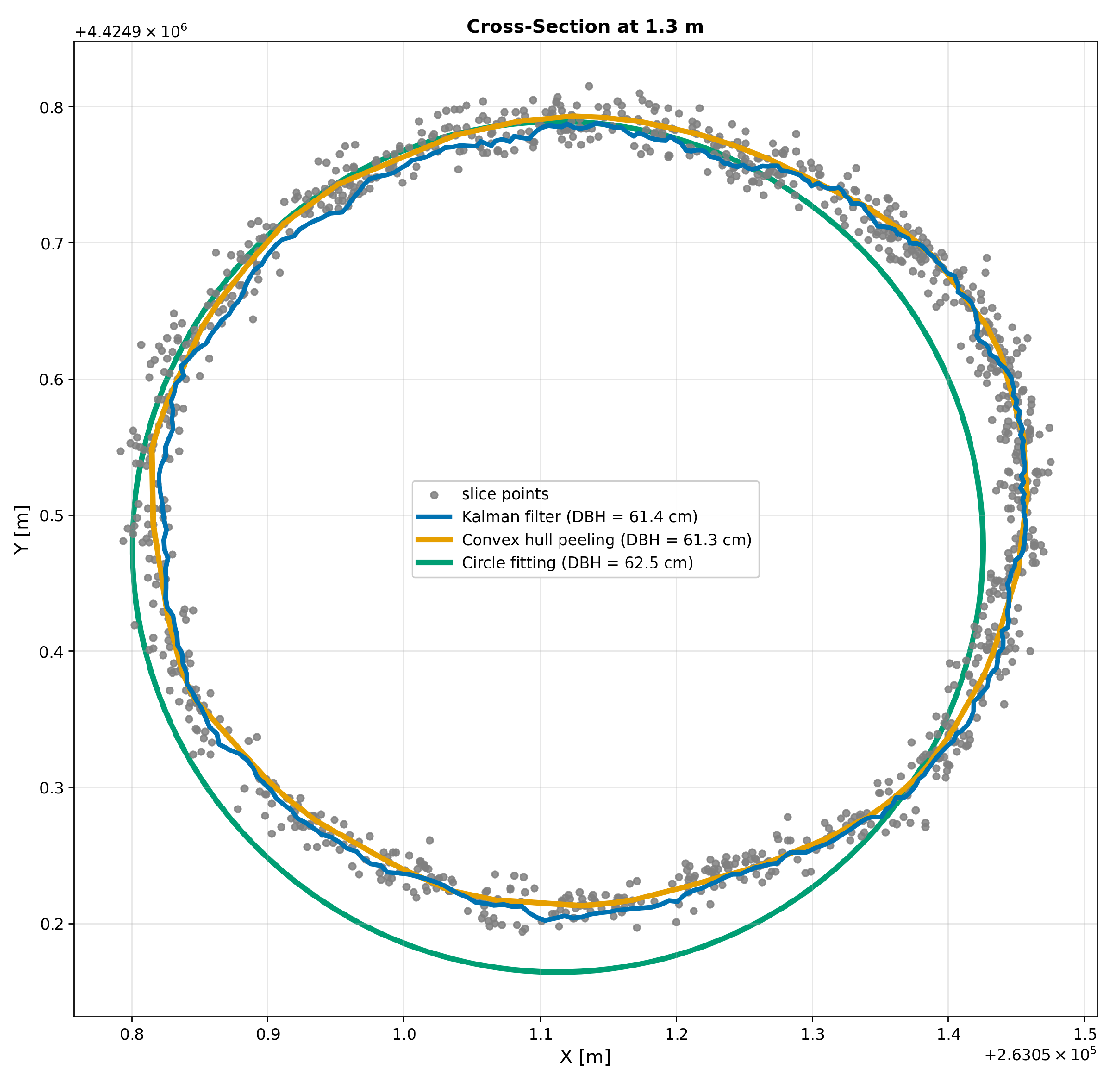
Figure A2.
Stem cross-section reconstruction for Tree ID 42 at a height of 1.3 m. Both the Kalman-based reconstruction and convex hull peeling show moderate deviations from the reference stem geometry, resulting in a moderate reconstruction error for both methods.
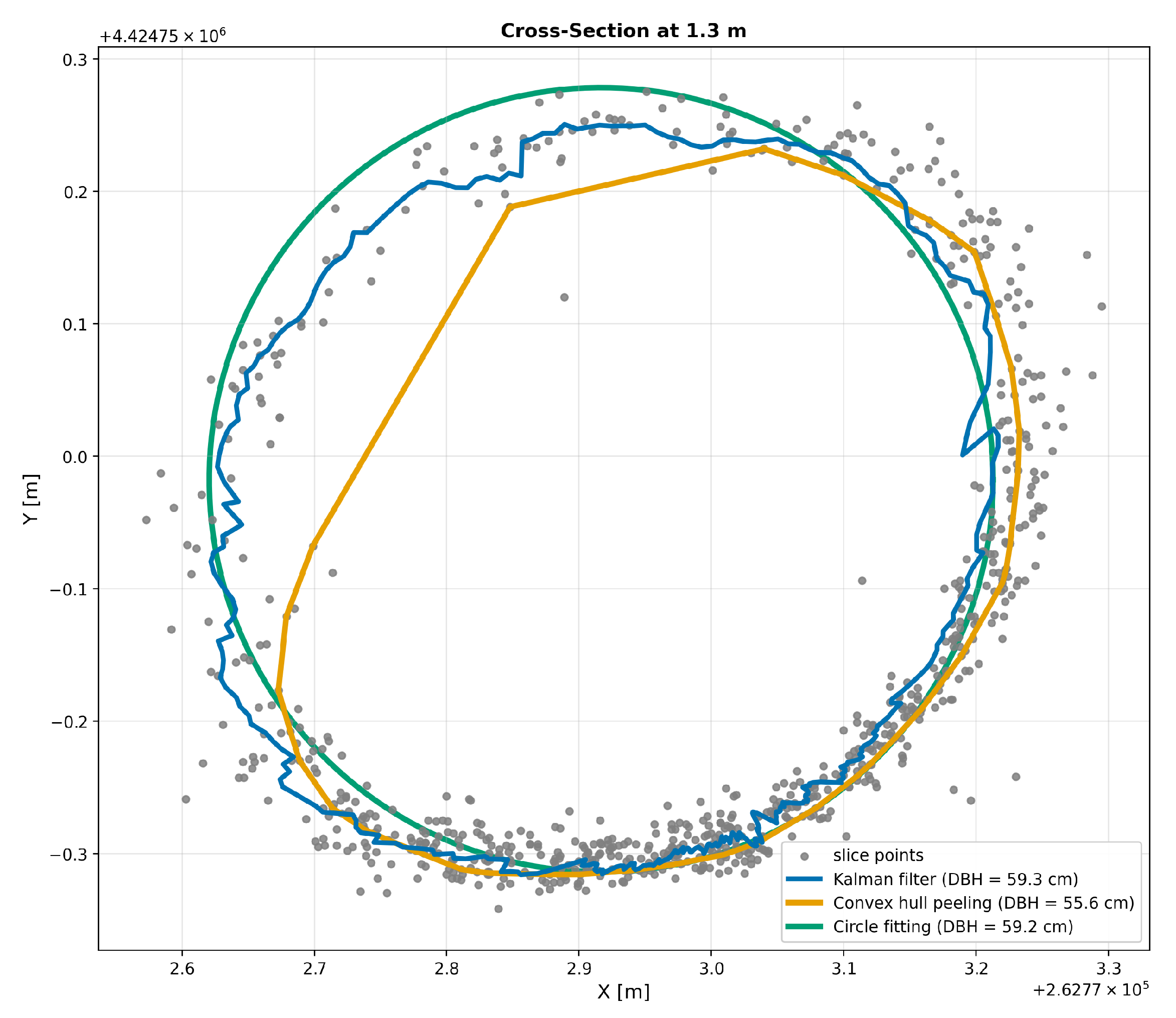
Figure A3.
Stem cross-section reconstruction for Tree ID 215 at a height of 1.3 m. Convex hull peeling accurately reconstructs the stem geometry with no noticeable error, whereas the Kalman-based reconstruction exhibits a pronounced deviation from the reference geometry.
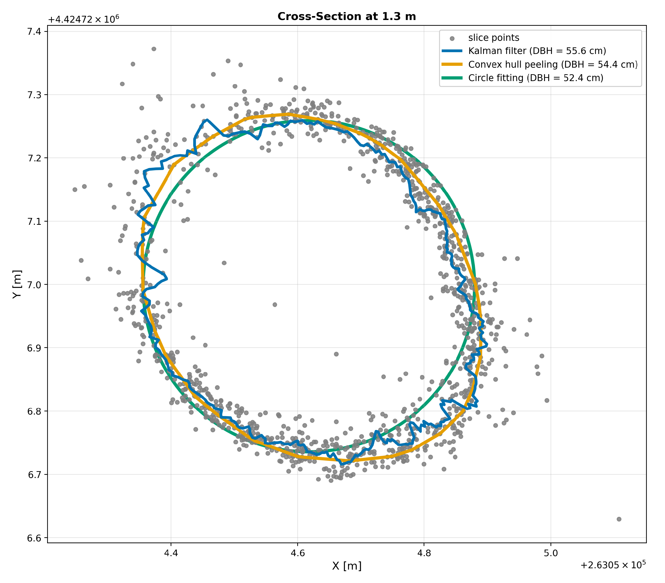
Figure A4.
Stem cross-section reconstruction for Tree ID 341 at a height of 1.3 m. The Kalman-based reconstruction shows only a slight deviation from the reference stem geometry, whereas convex hull peeling exhibits a pronounced reconstruction error.
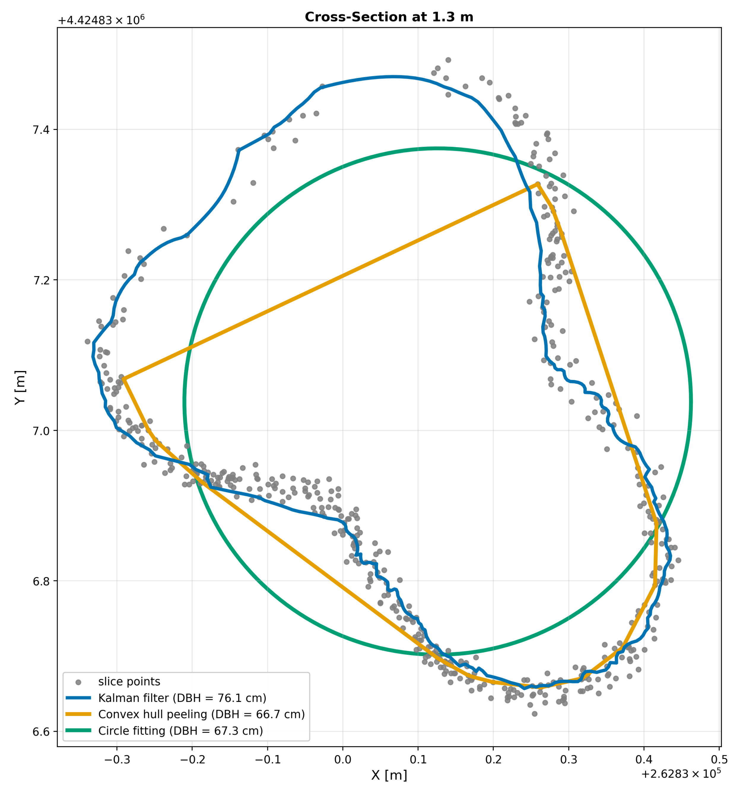
References
- Myers, N.; Mittermeier, R.A.; Mittermeier, C.G.; Da Fonseca, G.A.B.; Kent, J. Biodiversity hotspots for conservation priorities. Nature 2000, 403, 853–858. [Google Scholar] [CrossRef] [Scilit] [PubMed]
- den Herder, M.; Moreno, G.; Mosquera-Losada, R.M.; Palma, J.H.N.; Sidiropoulou, A.; Santiago Freijanes, J.J.; Crous-Duran, J.; Paulo, J.A.; Tomé, M.; Pantera, A.; et al. Current extent and stratification of agroforestry in the European Union. Agric. Ecosyst. Environ. 2017, 241, 121–132. [Google Scholar] [CrossRef] [Scilit]
- Plieninger, T.; Hartel, T.; Martín-López, B.; Beaufoy, G.; Bergmeier, E.; Kirby, K.; Montero, M.J.; Moreno, G.; Oteros-Rozas, E.; Van Uytvanck, J. Wood-pastures of Europe: Geographic coverage, social–ecological values, conservation management, and policy implications. Biol. Conserv. 2015, 190, 70–79. [Google Scholar] [CrossRef] [Scilit]
- Manning, A.D.; Fischer, J.; Lindenmayer, D.B. Scattered trees are keystone structures—Implications for conservation. Biol. Conserv. 2006, 132, 311–321. [Google Scholar] [CrossRef] [Scilit]
- Gea-Izquierdo, G.; Natalini, F.; Cardillo, E. Holm oak death is accelerated but not sudden and expresses drought legacies. Sci. Total. Environ. 2021, 754, 141793. [Google Scholar] [CrossRef] [Scilit] [PubMed]
- Bussotti, F.; Potočić, N.; Timmermann, V.; Lehmann, M.M.; Pollastrini, M. Tree crown defoliation in forest monitoring: Concepts, findings, and new perspectives for a physiological approach in the face of climate change. For. Int. J. For. Res. 2024, 97, 194–212. [Google Scholar] [CrossRef] [Scilit]
- Zhao, G. Plant compensatory growth: Its mechanisms and implications to agricultural sustainability under global environmental changes. Int. J. Sustain. Dev. World Ecol. 2024, 31, 348–360. [Google Scholar] [CrossRef] [Scilit]
- West, P.W. Tree and Forest Measurement, 3rd ed.; Springer: Cham, Switzerland, 2015. [Google Scholar] [CrossRef] [Scilit]
- Pandey, P.C.; Arellano, P. Introduction to forest monitoring using advanced remote sensing technology: An editorial message. In Advances in Remote Sensing for Forest Monitoring; Pandey, P.C., Arellano, P., Eds.; John Wiley & Sons: Hoboken, NJ, USA, 2022; pp. 1–9. [Google Scholar] [CrossRef] [Scilit]
- Calders, K.; Adams, J.; Armston, J.; Bartholomeus, H.; Bauwens, S.; Bentley, L.P.; Chave, J.; Danson, F.M.; Demol, M.; Disney, M.; et al. Terrestrial laser scanning in forest ecology: Expanding the horizon. Remote Sens. Environ. 2020, 251, 112102. [Google Scholar] [CrossRef] [Scilit]
- Vandendaele, B.; Martin-Ducup, O.; Fournier, R.A.; Pelletier, G.; Lejeune, P. Mobile Laser Scanning for Estimating Tree Structural Attributes in a Temperate Hardwood Forest. Remote Sens. 2022, 14, 4522. [Google Scholar] [CrossRef] [Scilit]
- Bogdanovich, E.; Perez-Priego, O.; El-Madany, T.S.; Guderle, M.; Pacheco-Labrador, J.; Levick, S.R.; Moreno, G.; Carrara, A.; Martín, M.P.; Migliavacca, M. Using terrestrial laser scanning for characterizing tree structural parameters and their changes under different management in a Mediterranean open woodland. For. Ecol. Manag. 2021, 486, 118945. [Google Scholar] [CrossRef] [Scilit]
- García, M.; Gajardo, J.; Riaño, D.; Zhao, K.; Martín, M.P.; Ustin, S. Canopy clumping appraisal using terrestrial and airborne laser scanning. Remote Sens. Environ. 2015, 161, 78–88. [Google Scholar] [CrossRef] [Scilit]
- Liang, X.; Kankare, V.; Hyyppä, J.; Wang, Y.; Kukko, A.; Haggrén, H.; Yu, X.; Kaartinen, H.; Jaakkola, A.; Guan, F.; et al. Terrestrial laser scanning in forest inventories. ISPRS J. Photogramm. Remote Sens. 2016, 115, 63–77. [Google Scholar] [CrossRef] [Scilit]
- Scalera, L.; Maset, E.; Tiozzo Fasiolo, D.; Bourr, K.; Cottiga, S.; De Lorenzo, A.; Carabin, G.; Alberti, G.; Gasparetto, A.; Mazzetto, F.; et al. Forest Surveying with Robotics and AI: SLAM-Based Mapping, Terrain-Aware Navigation, and Tree Parameter Estimation. Machines 2026, 14, 99. [Google Scholar] [CrossRef] [Scilit]
- Gollob, C.; Ritter, T.; Nothdurft, A. Forest Inventory with Long Range and High-Speed Personal Laser Scanning (PLS) and Simultaneous Localization and Mapping (SLAM) Technology. Remote Sens. 2020, 12, 1509. [Google Scholar] [CrossRef] [Scilit]
- Hyyppä, E.; Yu, X.; Kaartinen, H.; Hakala, T.; Kukko, A.; Vastaranta, M.; Hyyppä, J. Comparison of Backpack, Handheld, Under-Canopy UAV, and Above-Canopy UAV Laser Scanning for Field Reference Data Collection in Boreal Forests. Remote Sens. 2020, 12, 3327. [Google Scholar] [CrossRef] [Scilit]
- Kükenbrink, D.; Marty, M.; Rehush, N.; Abegg, M.; Ginzler, C. Evaluating the potential of handheld mobile laser scanning for an operational inclusion in a national forest inventory—A Swiss case study. Remote Sens. Environ. 2025, 321, 114685. [Google Scholar] [CrossRef] [Scilit]
- Duncanson, L.; Dubayah, R. Monitoring individual tree-based change with airborne lidar. Ecol. Evol. 2018, 8, 5079–5089. [Google Scholar] [CrossRef] [Scilit] [PubMed]
- Roussel, J.R.; Béland, M.; Caspersen, J.; Achim, A. A mathematical framework to describe the effect of beam incidence angle on metrics derived from airborne LiDAR: The case of forest canopies approaching turbid medium behaviour. Remote Sens. Environ. 2018, 209, 824–834. [Google Scholar] [CrossRef] [Scilit]
- Chirici, G.; Giannetti, F.; D’Amico, G.; Vangi, E.; Francini, S.; Borghi, C.; Corona, P.; Travaglini, D. Robotics in Forest Inventories: SPOT’s First Steps. Forests 2023, 14, 2170. [Google Scholar] [CrossRef] [Scilit]
- de Simone, L.; Fanfarillo, E.; Maccherini, S.; Fiaschi, T.; Alfonso, G.; Angelini, F.; Garabini, M.; Angiolini, C. One small step for a robot, one giant leap for habitat monitoring: A structural survey of EU forest habitats with robotically-mounted mobile laser scanning. Ecol. Indic. 2024, 160, 111882. [Google Scholar] [CrossRef] [Scilit]
- Mattamala, M.; Chebrolu, N.; Frey, J.; Freißmuth, L.; Oh, H.; Casseau, B.; Hutter, M.; Fallon, M. Building Forest Inventories With Autonomous Legged Robots – System, Lessons, and Challenges Ahead. IEEE Trans. Field Robot. 2025, 2, 418–436. [Google Scholar] [CrossRef] [Scilit]
- Moeller, R.; Deemyad, T.; Sebastian, A. Autonomous Navigation of an Agricultural Robot Using RTK GPS and Pixhawk. In Proceedings of the 2020 Intermountain Engineering, Technology and Computing (IETC), Orem, UT, USA, 2–3 October 2020; pp. 1–6. [Google Scholar] [CrossRef] [Scilit]
- Joffre, R.; Rambal, S.; Ratte, J.P. The dehesa system of southern Spain and Portugal as a natural ecosystem mimic. Agrofor. Syst. 1999, 45, 57–79. [Google Scholar] [CrossRef] [Scilit]
- Pinto-Correia, T.; Ribeiro, N.; Sá-Sousa, P. Introducing the montado, the cork and holm oak agroforestry system of Southern Portugal. Agrofor. Syst. 2011, 82, 99–104. [Google Scholar] [CrossRef] [Scilit]
- da Clara, M.I.E.; de Almeida Ribeiro, N.M.C. Decline of Mediterranean oak trees and its association with Phytophthora cinnamomi: A review. Eur. J. For. Res. 2013, 132, 411–432. [Google Scholar] [CrossRef] [Scilit]
- Plieninger, T.; Pulido, F.J.; Konold, W. Effects of land-use history on size structure of holm oak stands in Spanish dehesas: Implications for conservation and restoration. Environ. Conserv. 2003, 30, 61–70. [Google Scholar] [CrossRef] [Scilit]
- Ramezani, M.; Khosoussi, K.; Catt, G.; Moghadam, P.; Williams, J.; Borges, P.; Pauling, F.; Kottege, N. Wildcat: Online Continuous-Time 3D Lidar-Inertial SLAM. arXiv 2022, arXiv:2205.12595. [Google Scholar] [CrossRef] [Scilit]
- Brokaw, N.; Thompson, J. The H for DBH. For. Ecol. Manag. 2000, 129, 89–91. [Google Scholar] [CrossRef] [Scilit]
- Price, C.A.; Schroeder, T.A.; Branoff, B.; Marcano-Vega, H.; Pillot-Torres, N.; Chaudry, M.; Ross, M.; Papeş, M.; Van Bloem, S. Evaluating tree biomass estimation in trans-Atlantic mangrove species: Comparing bole diameter measurements for improved accuracy. PLoS ONE 2025, 20, e0323926. [Google Scholar] [CrossRef] [Scilit] [PubMed]
- Magarik, Y.A.S. “Roughly Speaking”: Why Do U.S. Foresters Measure DBH at 4.5 Feet? Soc. Nat. Resour. 2021, 34, 725–744. [Google Scholar] [CrossRef] [Scilit]
- Pinchot, G. A Primer of Forestry. Part I: The Forest; United States Division of Forestry, Bulletin No. 24; Government Printing Office: Washington, DC, USA, 1899. [Google Scholar]
- Magarik, Y.A.S.; Roman, L.A.; Henning, J.G. How should we measure the DBH of multi-stemmed urban trees? Urban For. Urban Green. 2020, 47, 126481. [Google Scholar] [CrossRef] [Scilit]
- Bilous, A.; Zadorozhniuk, R.; Makarevych, A.; Svynchuk, V.; Lashko, A.; Bilous, M.; Myroniuk, V.; Matsala, M. Sampling Protocol for Measuring Mean Diameter at Breast Height of Forked Urban Trees. Forests 2024, 15, 458. [Google Scholar] [CrossRef] [Scilit]
- Fonsêca, N.C.; Cunha, J.S.A.; da Cunha, J.A.S.; Santos, J.N.B.; Rodrigues, L.d.S.; Lins-e Silva, A.C.B. Tree Diametric Relationships and Their Implications for Estimation of Above-ground Biomass in a Tropical Rainforest. J. Sustain. For. 2022, 41, 999–1013. [Google Scholar] [CrossRef] [Scilit]
- Zhang, K.; Chen, S.C.; Whitman, D.; Shyu, M.L.; Yan, J.; Zhang, C. A progressive morphological filter for removing nonground measurements from airborne LIDAR data. IEEE Trans. Geosci. Remote Sens. 2003, 41, 872–882. [Google Scholar] [CrossRef] [Scilit]
- Wang, C.; Yang, X.; Xi, X.; Nie, S.; Dong, P. Introduction to LiDAR Remote Sensing, 1st ed.; CRC Press: Boca Raton, FL, USA, 2024. [Google Scholar] [CrossRef] [Scilit]
- Irwin, L.A.K.; Coops, N.C.; Riofrío, J.; Grubinger, S.G.; Barbeito, I.; Achim, A.; Roeser, D. Prioritizing commercial thinning: Quantification of growth and competition with high-density drone laser scanning. For. Int. J. For. Res. 2025, 98, 293–307. [Google Scholar] [CrossRef] [Scilit]
- Tao, S.; Wu, F.; Guo, Q.; Wang, Y.; Li, W.; Xue, B.; Hu, X.; Li, P.; Tian, D.; Li, C. Segmenting tree crowns from terrestrial and mobile LiDAR data by exploring ecological theories. ISPRS J. Photogramm. Remote Sens. 2015, 110, 66–76. [Google Scholar] [CrossRef] [Scilit]
- Liu, J.; Skidmore, A.K.; Heurich, M.; Wang, T. Significant effect of topographic normalization of airborne LiDAR data on the retrieval of plant area index profile in mountainous forests. ISPRS J. Photogramm. Remote Sens. 2017, 132, 77–87. [Google Scholar] [CrossRef] [Scilit]
- Coope, I.D. Circle fitting by linear and nonlinear least squares. J. Optim. Theory Appl. 1993, 76, 381–388. [Google Scholar] [CrossRef] [Scilit]
- Stovall, A.E.L.; Vorster, A.G.; Anderson, R.S.; Evangelista, P.H.; Shugart, H.H. Non-destructive aboveground biomass estimation of coniferous trees using terrestrial LiDAR. Remote Sens. Environ. 2017, 200, 31–42. [Google Scholar] [CrossRef] [Scilit]
- Cai, S.; Pang, Y. Trunk cross-section reconstruction and DBH calculation from handheld laser scanning data using Kalman filter. J. For. Res. 2025, 37, 12. [Google Scholar] [CrossRef] [Scilit]
- Mîzgaciu, L.; Tudoran, G.M.; Ciocan, A.E.; Stăncioiu, P.T.; Niţă, M.D. A Comparative Analysis of UAV LiDAR and Mobile Laser Scanning for Tree Height and DBH Estimation in a Structurally Complex, Mixed-Species Natural Forest. Forests 2025, 16, 1481. [Google Scholar] [CrossRef] [Scilit]
- Sofia, S.; Giannetti, F.; Buscarini, S.; Chirici, G.; Corezzola, S.; Maetzke, F.G.; Miozzo, M.; Travaglini, D.; La Mela Veca, D.S. Comparing efficiency, timing and costs of different walking paths in HMLS LiDAR survey. Ann. For. Res. 2024, 67, 87–107. [Google Scholar] [CrossRef] [Scilit]
- Kuželka, K.; Marušák, R.; Surový, P. Inventory of close-to-nature forest stands using terrestrial mobile laser scanning. Int. J. Appl. Earth Obs. Geoinf. 2022, 115, 103104. [Google Scholar] [CrossRef] [Scilit]
- Campelo, F.; Ribas, M.; Gutiérrez, E. Plastic bimodal growth in a Mediterranean mixed-forest of Quercus ilex and Pinus halepensis. Dendrochronologia 2021, 67, 125836. [Google Scholar] [CrossRef] [Scilit]
- Costa, A.; Moreira, A.C. Stem diameter decrement in holm oak (Quercus rotundifolia Lam.): Insights into tree decline pathways in endangered woodlands of Southern Portugal. Ecologies 2023, 4, 229–241. [Google Scholar] [CrossRef] [Scilit]
- Bater, C.W.; Wulder, M.A.; Coops, N.C.; Nelson, R.F.; Hilker, T.; Næsset, E. Stability of sample-based scanning-LiDAR-derived vegetation metrics for forest monitoring. IEEE Trans. Geosci. Remote Sens. 2011, 49, 2385–2392. [Google Scholar] [CrossRef] [Scilit]
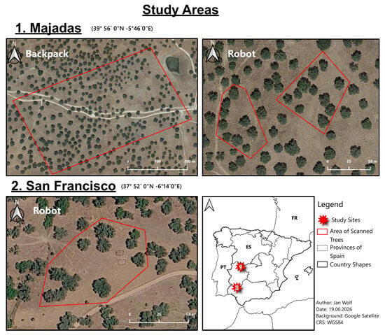
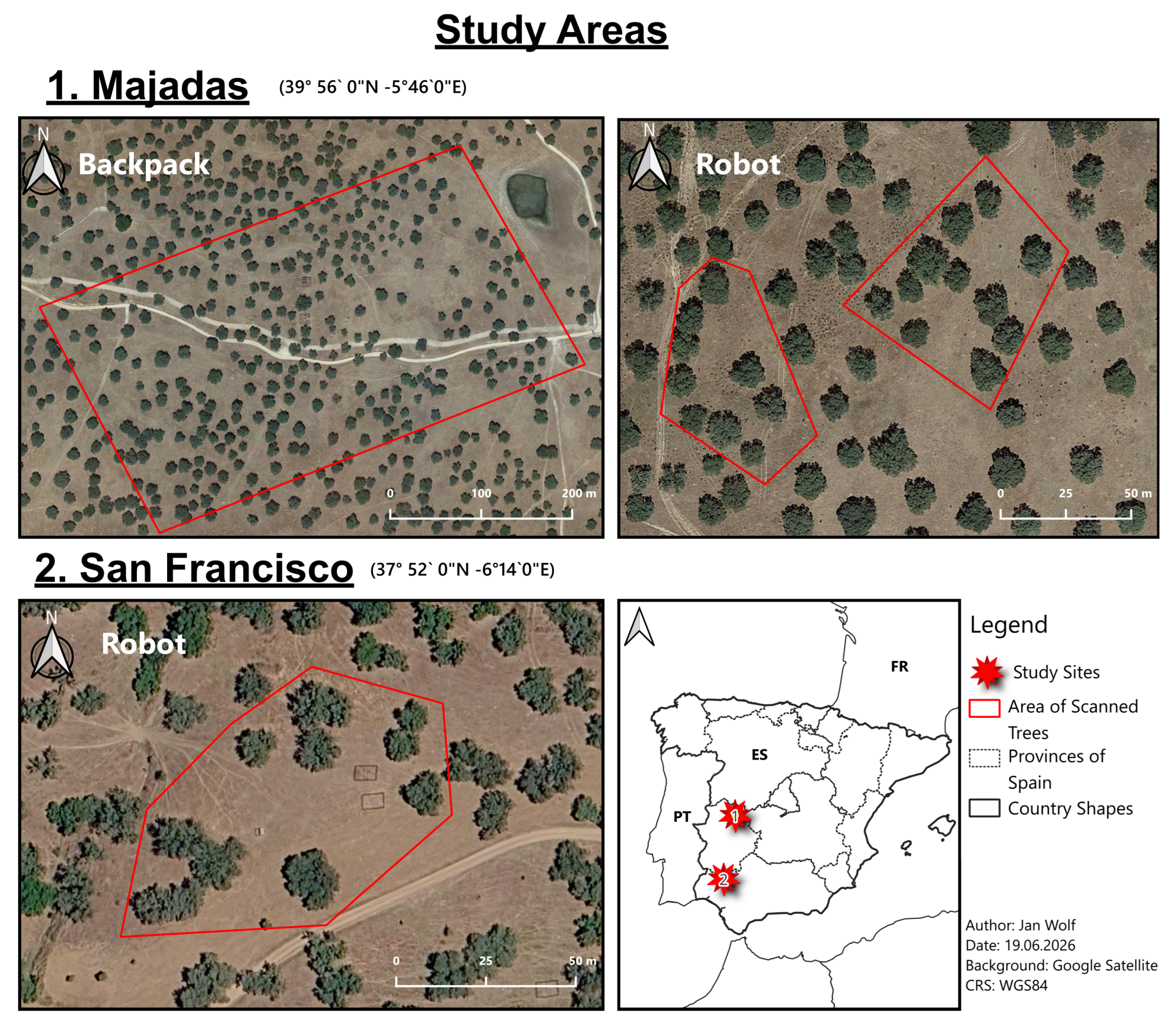
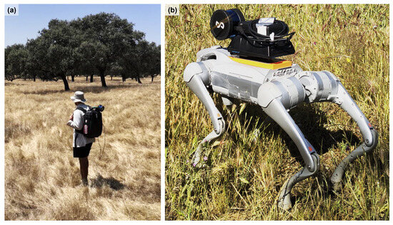
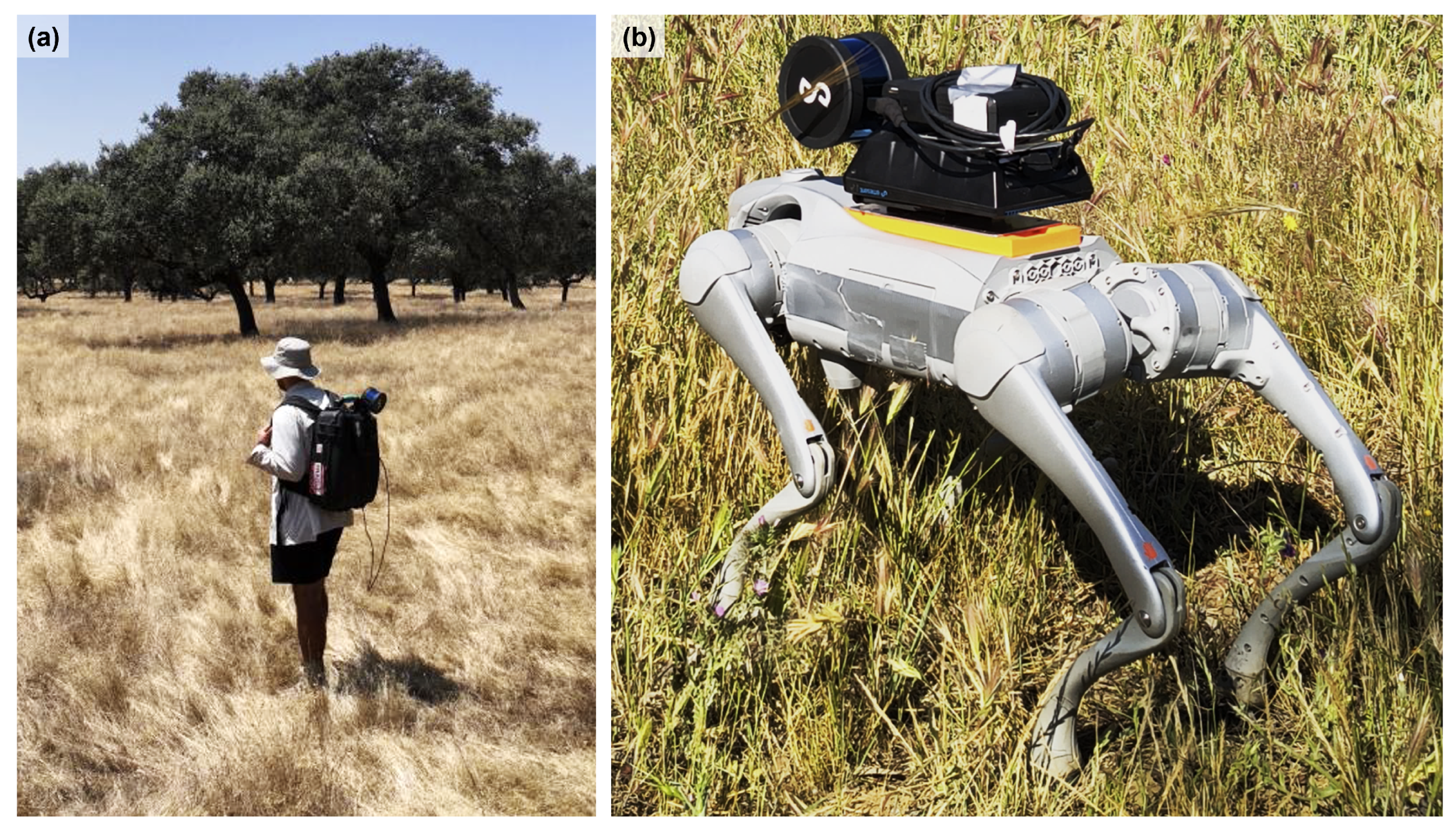
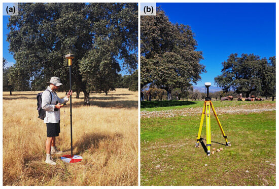
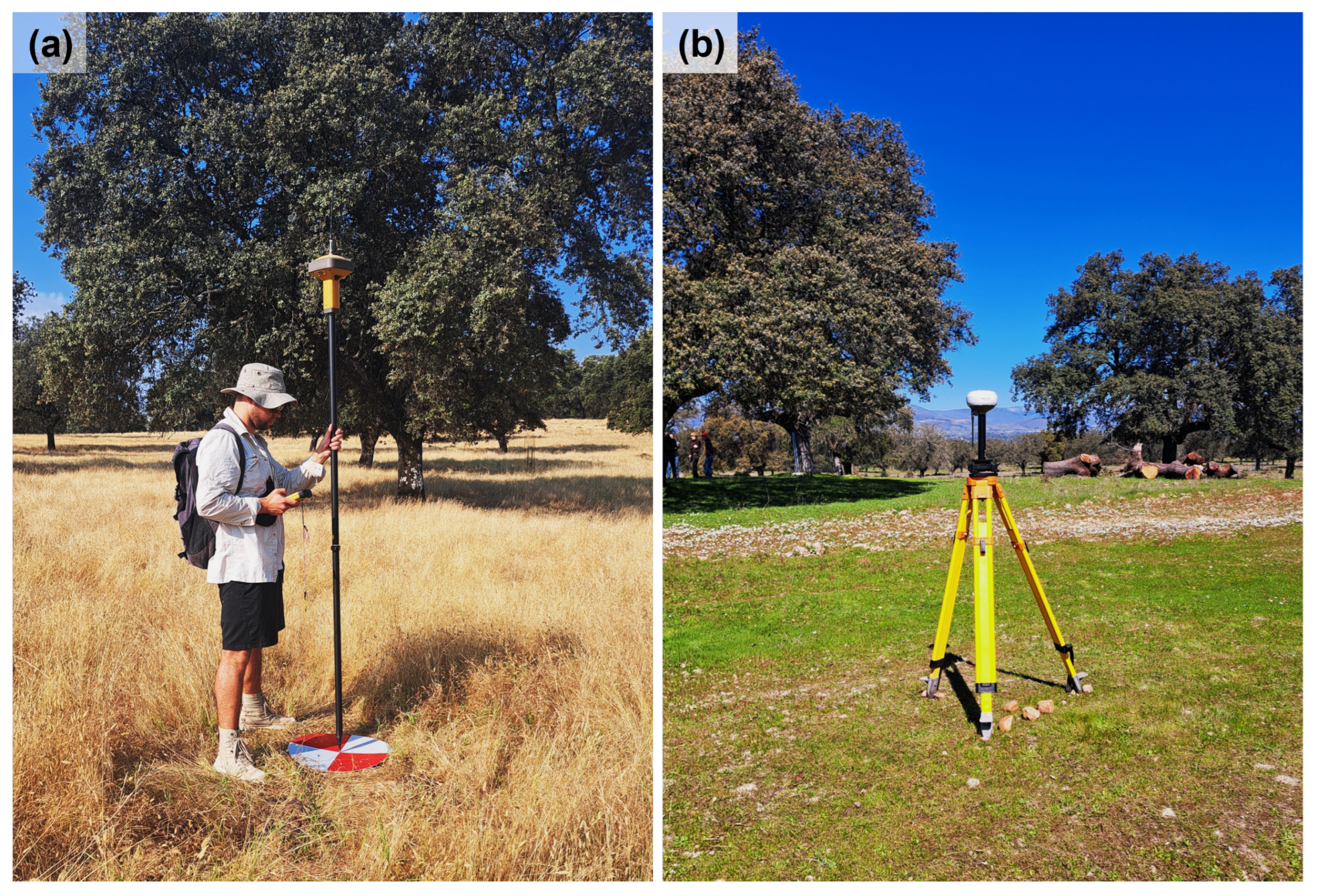
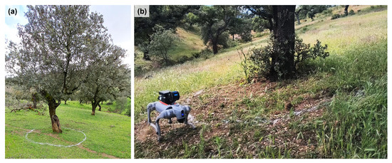
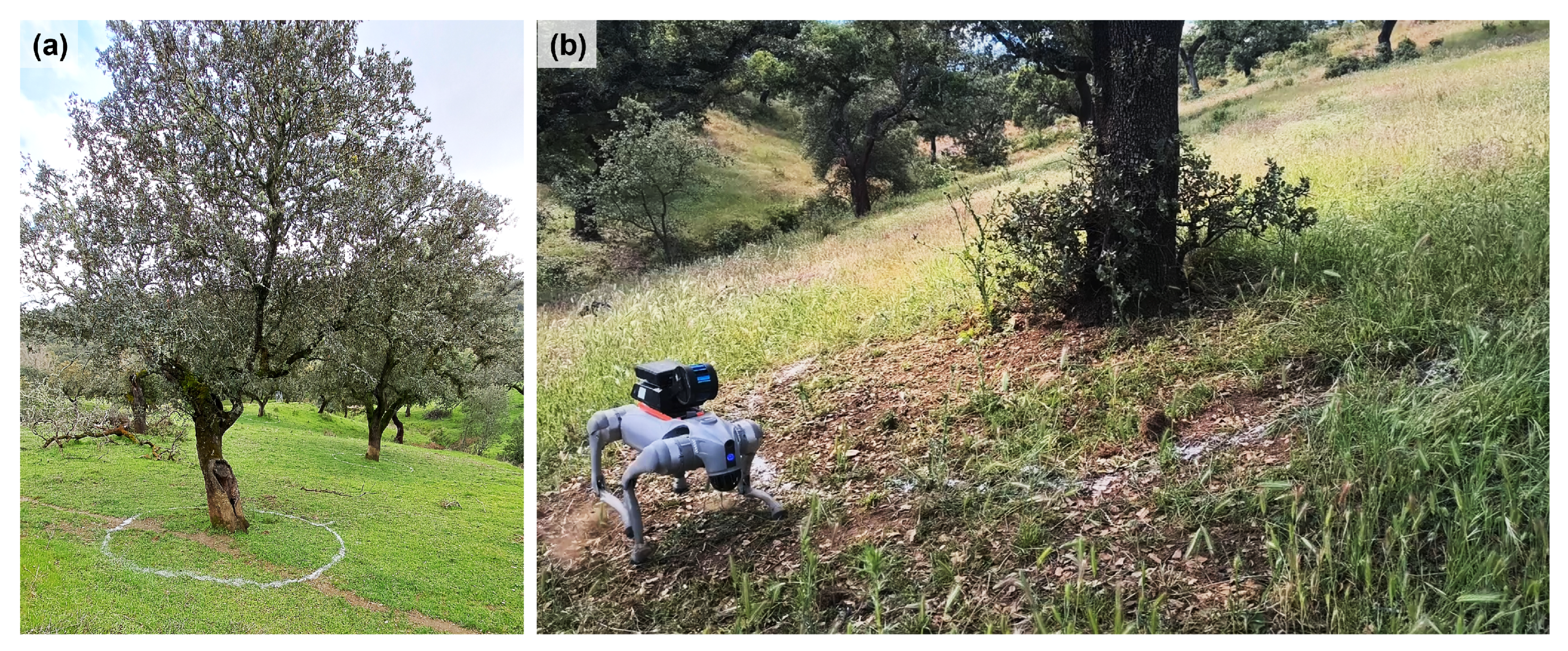
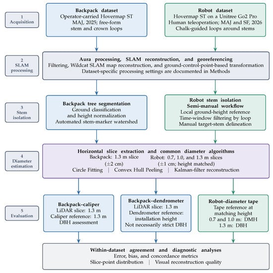
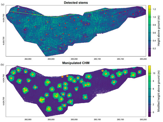
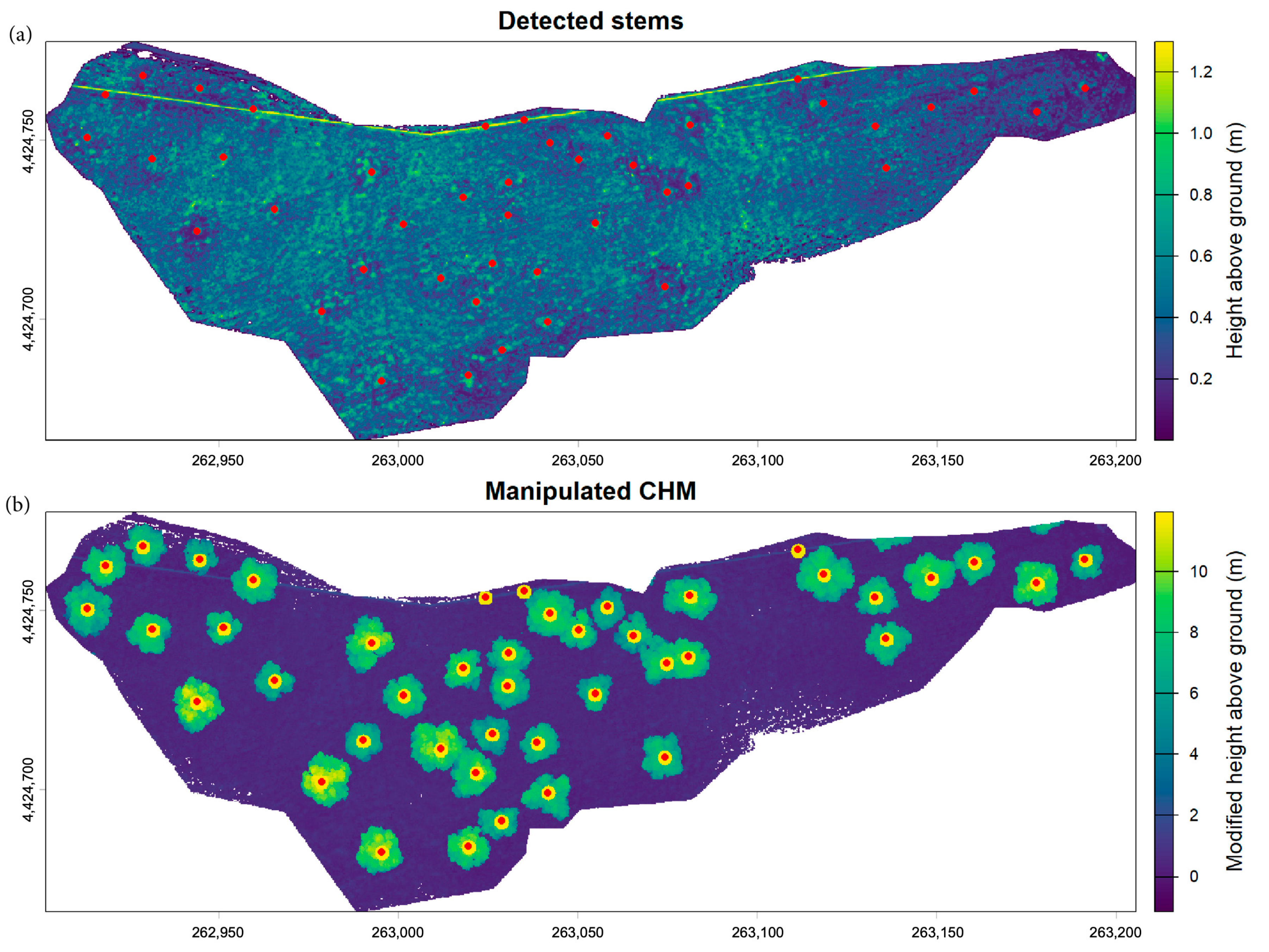
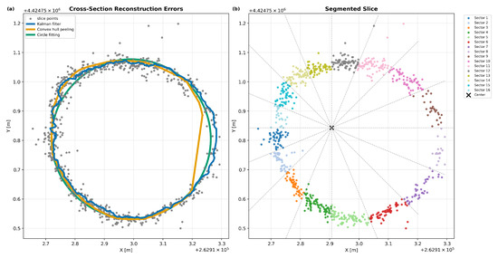
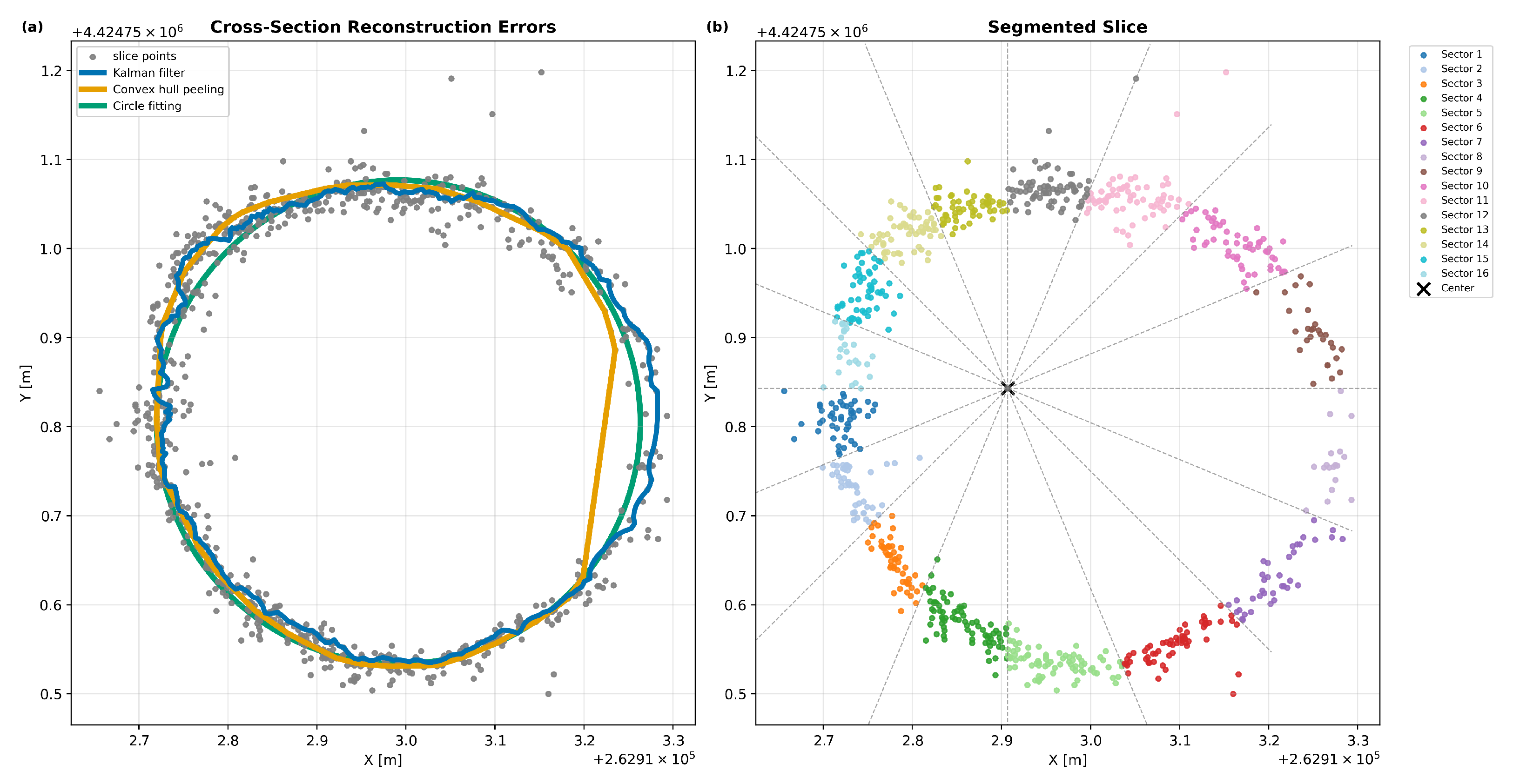
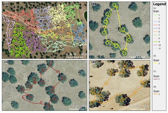
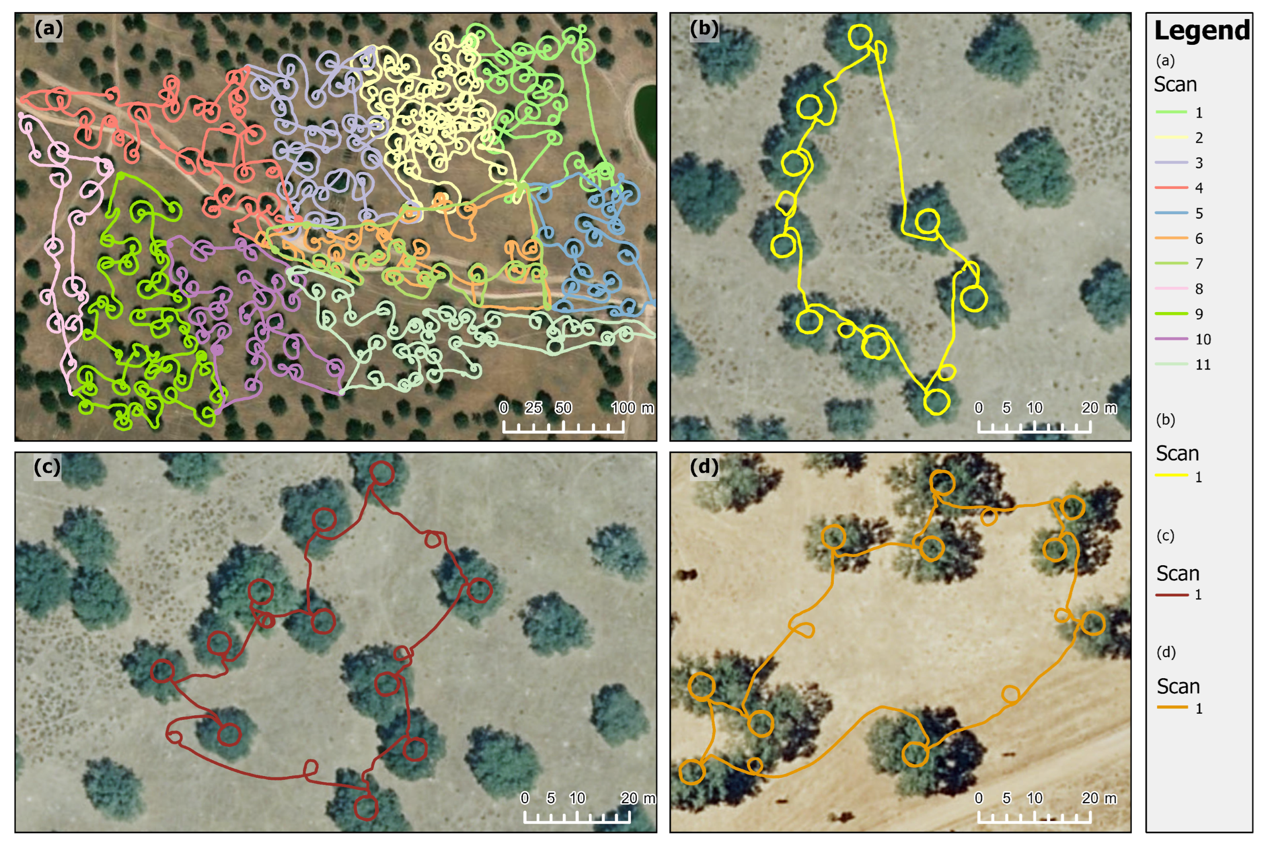
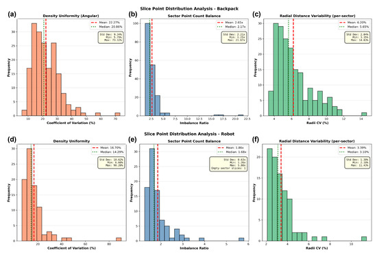
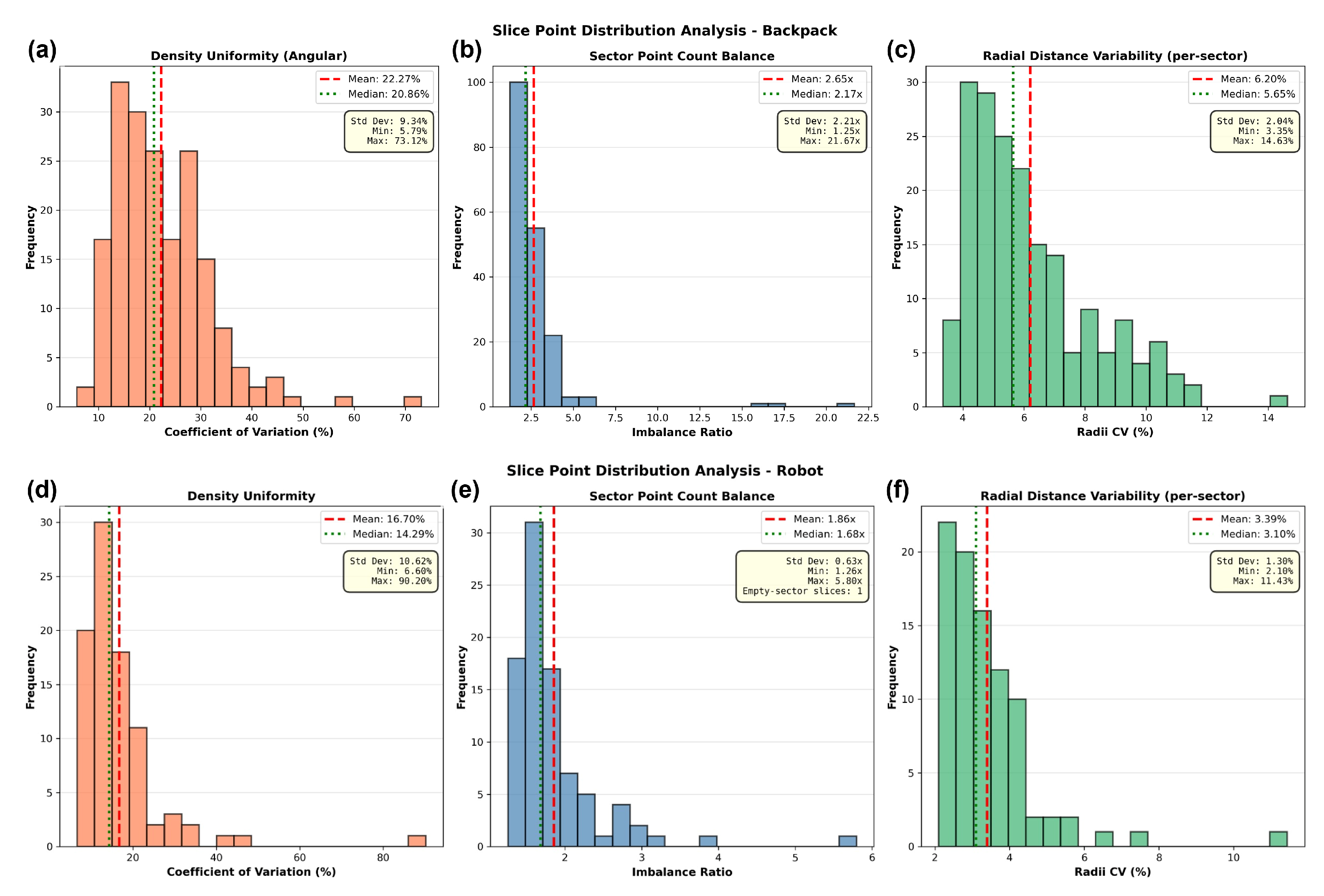
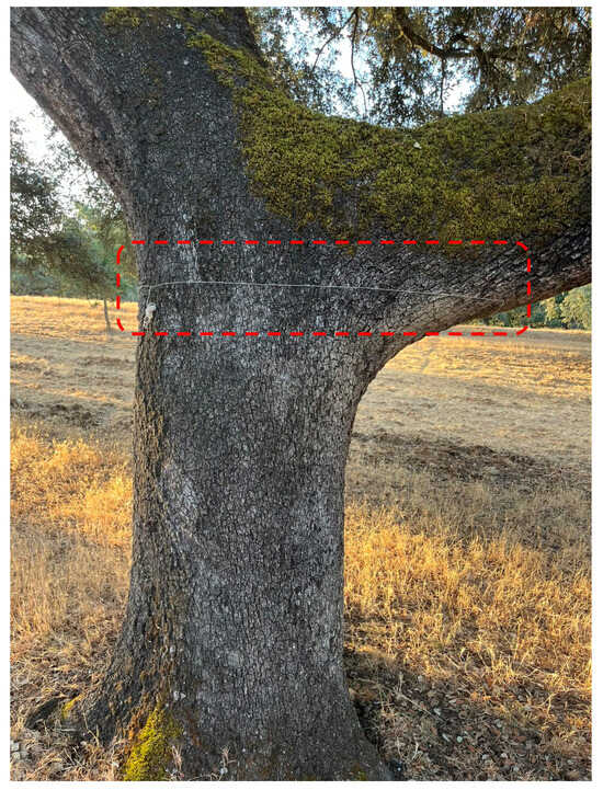
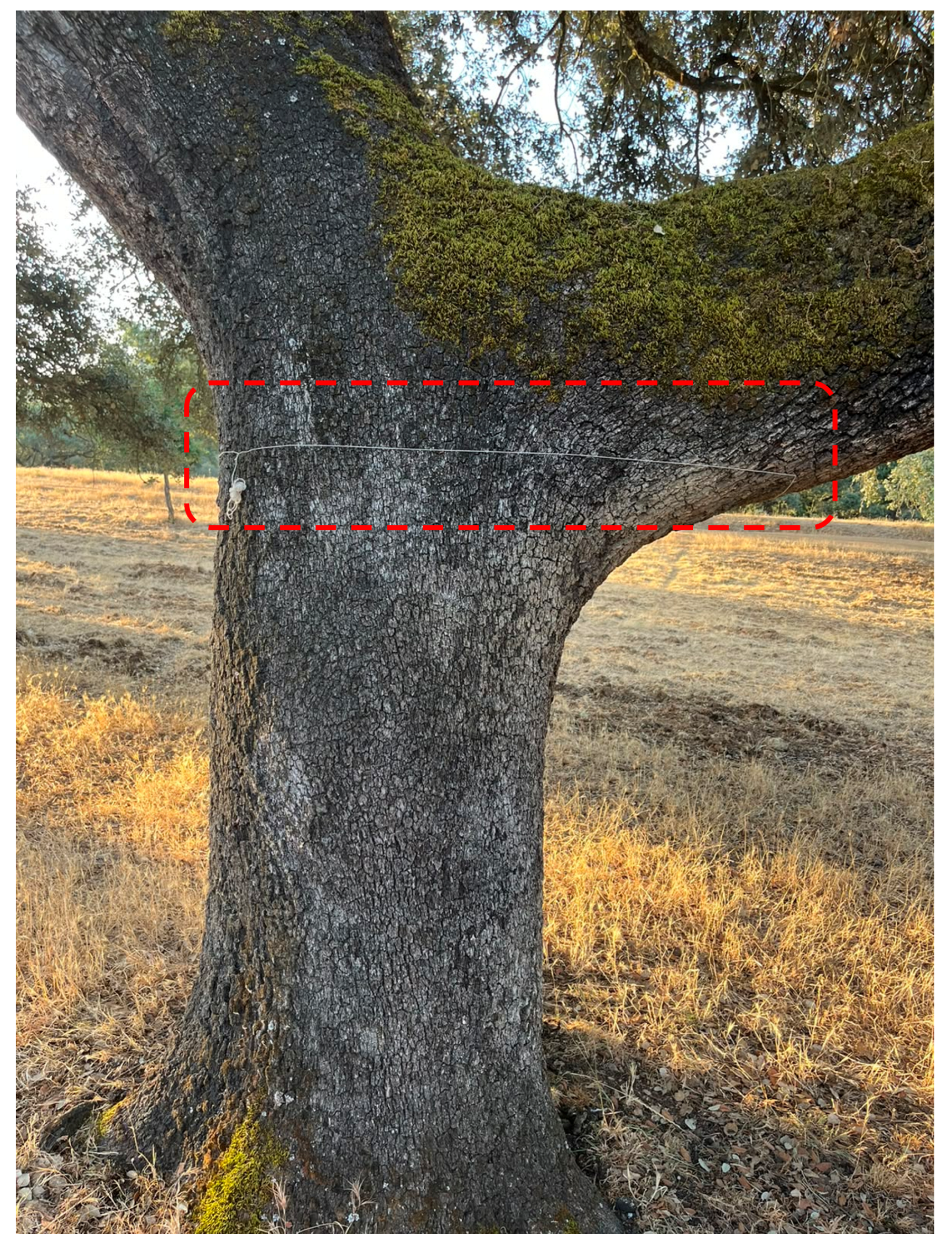
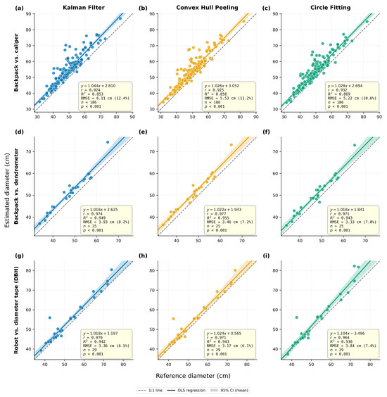
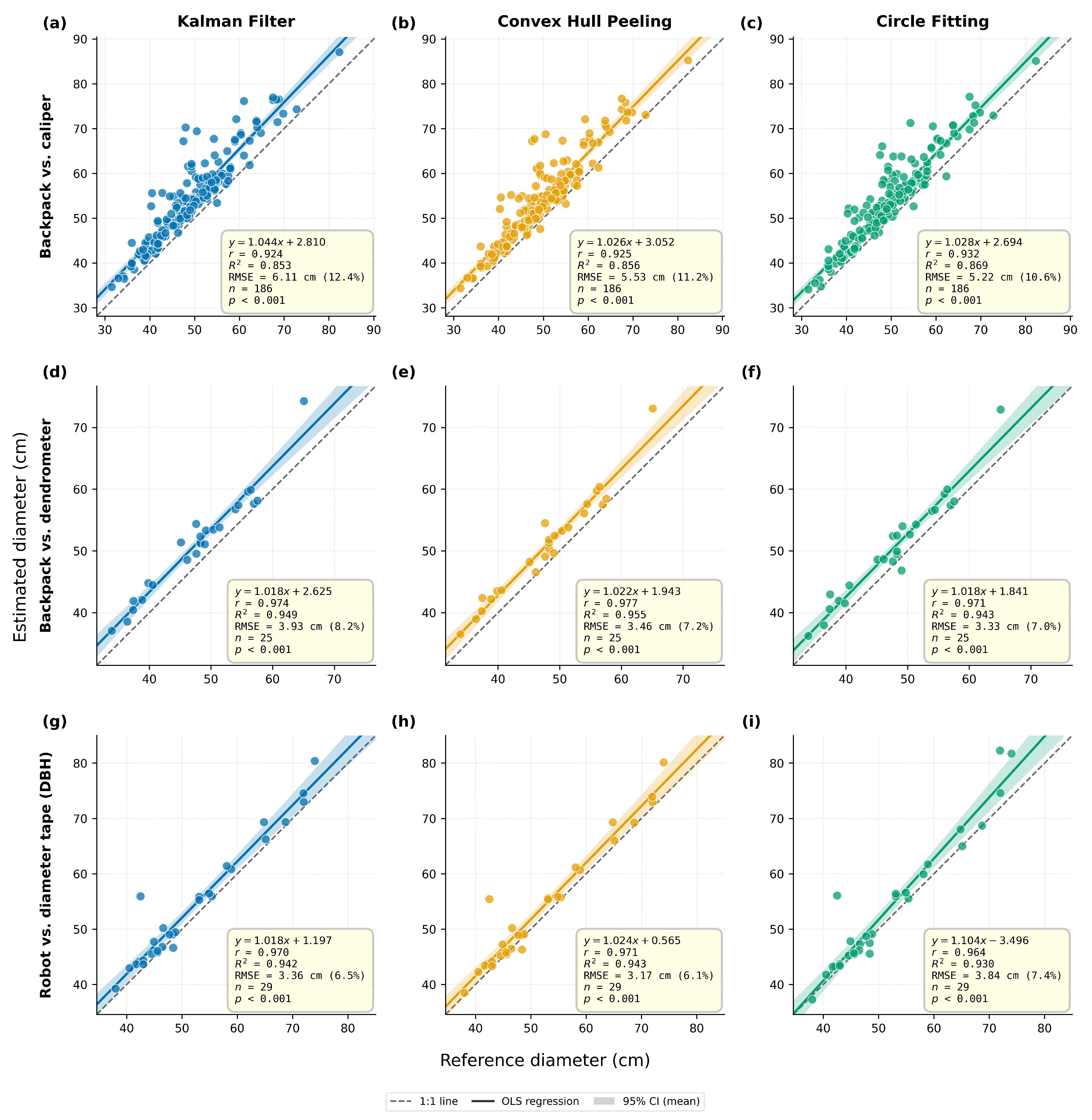
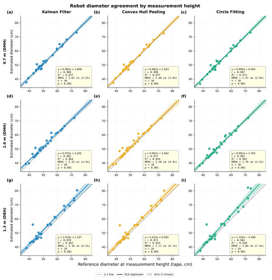
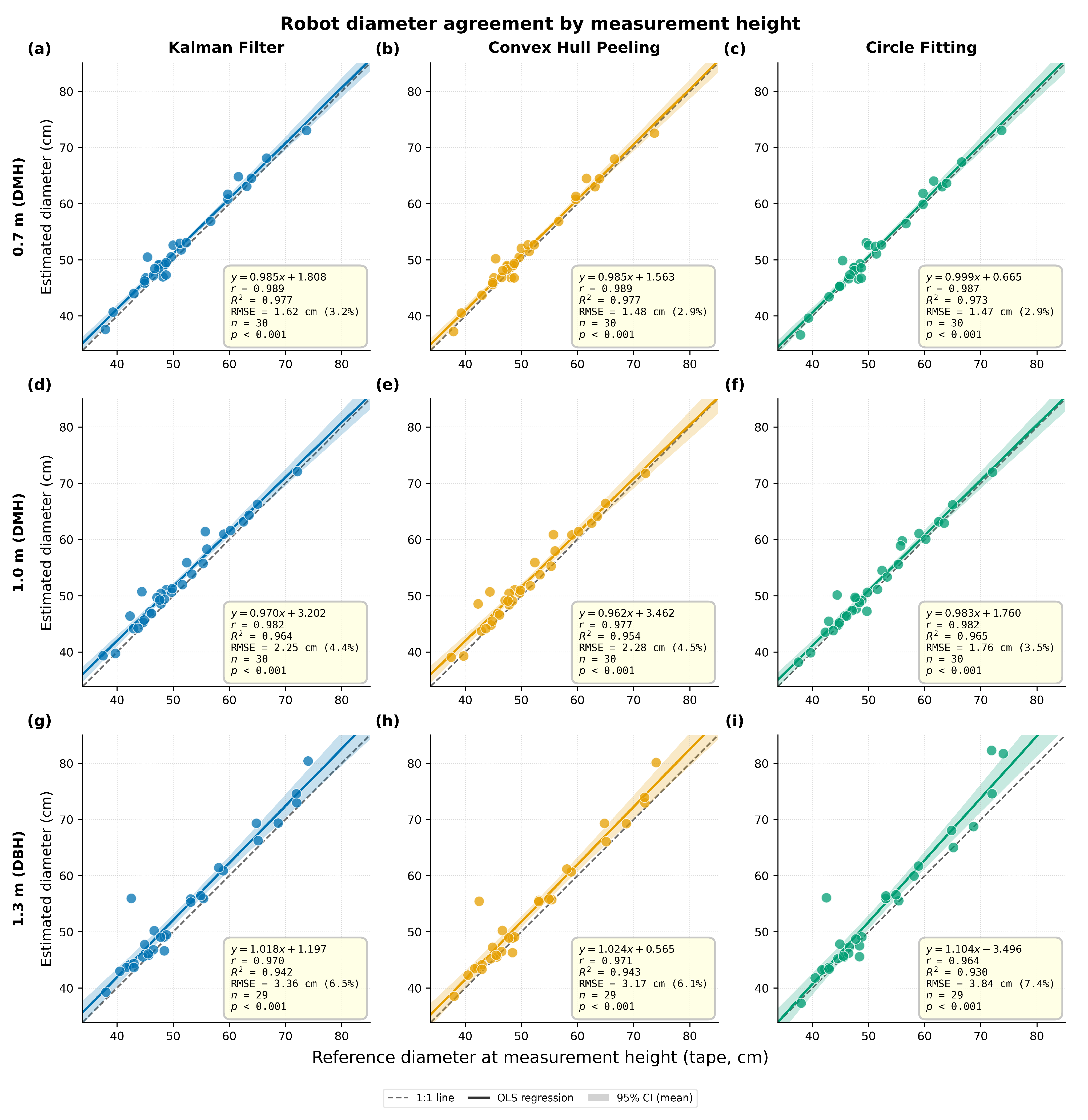
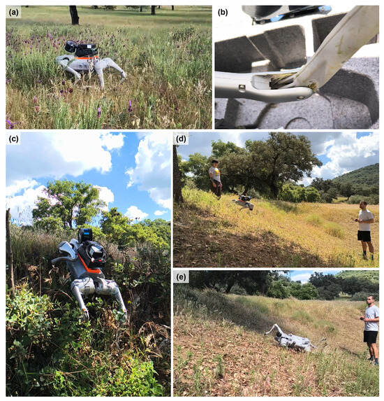
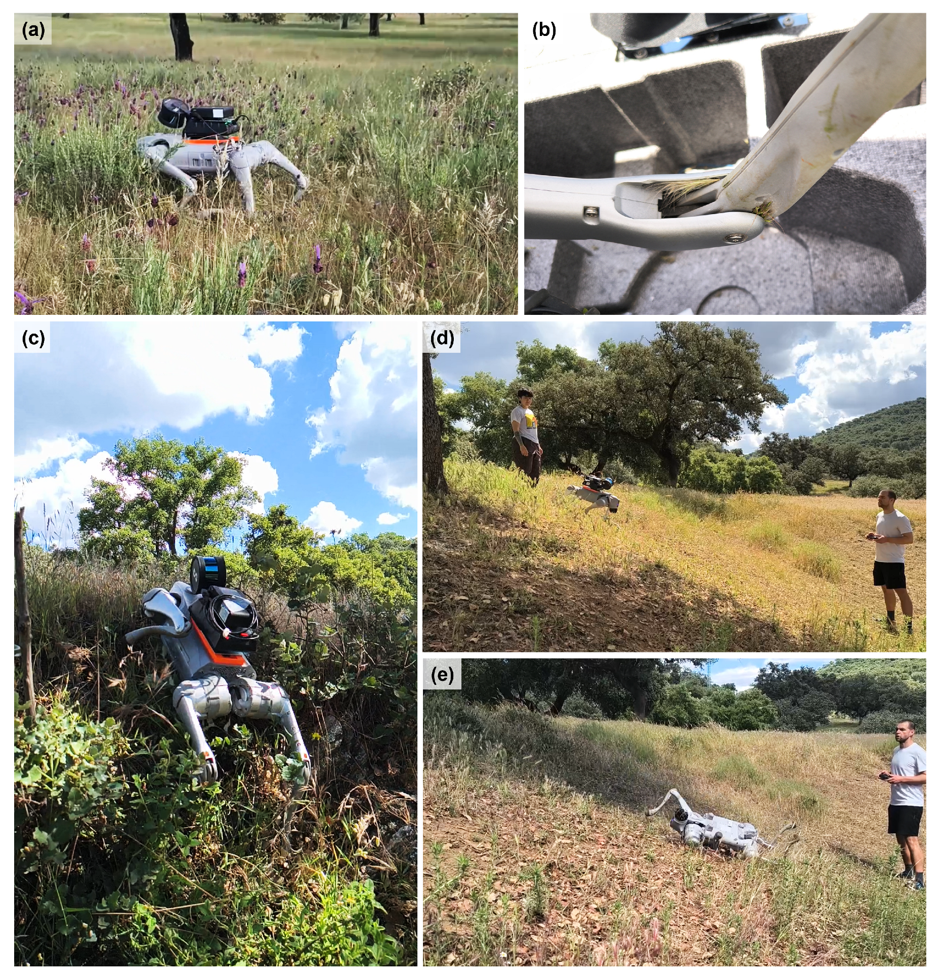

Disclaimer/Publisher’s Note: The statements, opinions and data contained in all publications are solely those of the individual author(s) and contributor(s) and not of MDPI and/or the editor(s). MDPI and/or the editor(s) disclaim responsibility for any injury to people or property resulting from any ideas, methods, instructions or products referred to in the content. |
© 2026 by the authors. Licensee MDPI, Basel, Switzerland. This article is an open access article distributed under the terms and conditions of the Creative Commons Attribution (CC BY) license.