Extension of an Efficient Approach for Spin-Angular Integrations in Atomic Structure Calculations

Abstract

In this study, an extension of the general method [G. Gaigalas, Z. Rudzikas, C. Froese Fischer, J. Phys. B, At. Mol. Phys. (1997). DOI: 10.1088/0953-4075/30/17/006] is described for finding algebraic expressions of the spin-angular parts of the reduced matrix elements of any one- and two-particle operator for an arbitrary number of shells in an atomic configuration. This extension is related, at first, to a change in the definition of tensor structure, where a non-scalar space with respect to l and s for any two-particle operator acts on four different shells. This leads to more efficient expressions for recoupling matrices and amplitudes, which are presented in the paper. In addition, the paper presents new expressions for some of the recoupling matrices, in which 6j- and 9j-coefficients are summed up algebraically. All this leads to a significantly simpler and faster calculation of the spin-angular parts of any non-scalar two-particle operator.

1. Introduction

This paper presents further development of the calculation methodology for the spin-angular part of the reduced matrix element. The methodology presented in this paper and in three previous papers [1,2,3] (hereinafter referred to as P1, P2, and P3) was developed in parallel with the development of the Atsp [4,5,6,7,8] (for the Atsp theoretical background, see [9,10]) and Grasp [11,12,13] (for the Grasp theoretical background, see [14]) computer packages, with particular attention paid to the calculation of the spin-angular part of reduced matrix elements. This part of the software was one of the weakest points in these computer packages (see for example [15]), especially in Atsp. The part of this package responsible for calculating the spin-angular parts was slow and, in some cases, e.g., when using Breit–Pauli operator [10] calculations, led to incorrect results. It became clear that, in order to successfully solve the problems mentioned above, it was necessary to review the theory of the calculation of spin-angular coefficients itself. It was determined that the most effective way to achieve the desired result was to create a new method for integrating spin-angular variables, based on the combination [1] of the angular momentum theory [16] as described in [17], the concept of irreducible tensorial sets [18,19,20], the generalized graphical approach [21], the second quantization in coupled tensorial form [20], the quasi-spin approach [22], and the use of reduced coefficients of fractional parentage [23,24].

Since the methodology was developed in parallel with the creation of the programs, initial attention was focused primarily on calculating reduced matrix elements for one- and two-particle scalar operators in the l and s spaces in the context of non-relativistic atomic theory, or in the j space in the context of relativistic atomic theory. As a result, the first part of the methodology was created and published in P2. The methodology was subsequently developed for a non-scalar one-particle operator, and this extension was published in P3. Moving on to more complex two-particle operators (non-scalar two-particle operators), such as spin–other–orbit and spin–spin [10], further development of the methodology was carried out, resulting in the most effective expressions for calculating the spin-angular coefficients of these operators. It is precisely this development that is presented in this article. This research in P1, P2, and P3 was conducted in close collaboration with Prof. Ian Philip Grant (1930–2025), Prof. Charlotte Froese Fischer (1929–2024), and Prof. Zenonas Rokus Rudzikas (1940–2011). This successful collaboration resulted in the creation of a new methodology, published in P1, P2 and P3, which formed the basis of new versions of Atsp [25] and Grasp [26,27] software packages. A detailed software library for calculating spin-angular reduction matrix elements has been published in [28] for relativistic atomic theory and is being prepared for publication in [29] for non-relativistic atomic theory.

The present paper is divided into an introduction, four sections, and a conclusion. Section 2 provides tensorial expressions for any non-scalar two-particle operator in the l and s spaces. Section 3 deals with reduced matrix elements of this non-scalar two-particle operator between complex configurations. Section 4 presents more efficient expressions for recoupling matrix elements. More efficient expressions for amplitude ${\Theta }^{\prime }\left(n_i{\lambda }_i,n_j{\lambda }_j,n_{i^{\prime }}{\lambda }_i^{\prime },n_j^{\prime }{\lambda }_j^{\prime },\Xi \right)$ are listed in Section 5. The expressions presented in these sections are also suitable for calculating the spin-angular parts of reduced matrix elements of any non-scalar two- or three-particle operator from relativistic atomic theory. Although they are not relevant for physical operators, they can be most appropriate for effective operators which appear, for example, in the perturbation theory [30]. The efficiency evaluation of the methodology presented in the current paper is provided in Section 6.

2. Tensorial Expressions for Any Non-Scalar Two-Particle Operators in l and s Spaces

In order to be able to find the expressions for the reduced matrix elements of the operators studied, we have to express these operators in terms of the irreducible tensors or their irreducible tensorial products. In this section we will present all the necessary tensorial expressions for any two-particle operator G.

First, we express the operator in second-quantization form as in P1:

$$\begin{array}{c}\hfill {\displaystyle G=\sum _{\begin{array}{c}\hfill n_i{l}_i,n_j{l}_j\\ \hfill n_{i^{\prime }}{l}_{i^{\prime }},n_{j^{\prime }}{l}_{j^{\prime }}\end{array}}\widehat{G}\left(n_i{l}_i{n}_j{l}_j{n}_i^{\prime }{l}_i^{\prime }{n}_j^{\prime }{l}_j^{\prime }\right)=\frac{1}{2}\sum _{i,j,i^{\prime },j^{\prime }}{a}_i{a}_j{a}_{j^{\prime }}^{†}{a}_{i^{\prime }}^{†}\left(i,j\left|g\right|i^{\prime },j^{\prime }\right)}\end{array}$$

(1)

where, as is customary, the creation operators $a_i{a}_j$ appear to the left of the annihilation operators $a_{j^{\prime }}^{†}{a}_{i^{\prime }}^{†}$ before defining the shells upon which the second-quantization operators are acting. It should be noted that in P1–P3 as well as in the current paper, the symbol of the complex conjugate is used to denote the electron annihilation operator rather than the creation operator. Such a definition was introduced by Dirac [31] and was followed by [20,22,32]. It is compatible with the definition used in tensorial algebra, as well as in Racah algebra for atomic theory.

After defining the shells explicitly in (1), the second-quantization operators are transformed using their commutation relations so that all operators with the same $n\lambda$ ($\lambda \equiv l,s$) are beside one another. For example, in the case where the electron creation operator $a_i$ (where $i\equiv n_i{l}_{i}s{m}_{l_i}{m}_{s_i}$) acts upon the same shell $\gamma$, the electron creation operator $a_j$ acts upon the same shell $\delta$, the electron annihilation operator $a_{i^{\prime }}^{†}$ acts upon the shell $\alpha$, and electron annihilation operator $a_{j^{\prime }}^{†}$ acts upon the same shell $\beta$, we have

$$\begin{array}{c}\hfill \widehat{G}\left(\gamma \delta \alpha \beta \right)\\ \hfill {\displaystyle =\frac{1}{2}\sum _{\begin{array}{c}{m}_{l_{\alpha }}{m}_{s_{\alpha }}\hfill \\ m_{l_{\beta }}{m}_{s_{\beta }}\hfill \end{array}}\sum _{\begin{array}{c}{m}_{l_{\gamma }}{m}_{s_{\gamma }}\hfill \\ m_{l_{\delta }}{m}_{s_{\delta }}\hfill \end{array}}{a}_{m_{l_{\alpha }}{m}_{s_{\alpha }}}^{†\left(l_{\alpha }{s}_{\alpha }\right)}{a}_{m_{l_{\beta }}{m}_{s_{\beta }}}^{†\left(l_{\beta }{s}_{\beta }\right)}{a}_{m_{l_{\gamma }}{m}_{s_{\gamma }}}^{\left(l_{\gamma }{s}_{\gamma }\right)}{a}_{m_{l_{\delta }}{m}_{s_{\delta }}}^{\left(l_{\delta }{s}_{\delta }\right)}\left(n_{\gamma }{\lambda }_{\gamma }{m}_{l_{\gamma }}{m}_{s_{\gamma }}{n}_{\delta }{\lambda }_{\delta }{m}_{l_{\delta }}{m}_{s_{\delta }}\left|g^{\left({\kappa }_1{\kappa }_{2}k,{\sigma }_1{\sigma }_{2}k\right)}\right|n_{\alpha }{\lambda }_{\alpha }{m}_{l_{\alpha }}{m}_{s_{\alpha }}{n}_{\beta }{\lambda }_{\beta }{m}_{l_{\beta }}{m}_{s_{\beta }}\right).}\end{array}$$

(2)

Here we imply that a tensorial structure indexed by $({\kappa }_1{\kappa }_{2}k,{\sigma }_1{\sigma }_{2}k)$ at g has rank ${\kappa }_1$ for electron 1, rank ${\kappa }_2$ for electron 2, a resulting rank k in the l space, and corresponding ranks ${\sigma }_1{\sigma }_{2}k$ in the s space.

Now, applying the graphical approach of angular momentum theory [21], we can get an expression, namely

$$\begin{array}{c}\hfill \widehat{G}\left(\gamma \delta \alpha \beta \right)\\ \hfill {\displaystyle =-\frac{1}{2}\sum _{{\kappa }_{12}{\sigma }_{12}}\sum _p{\left(-1\right)}^{l_{\alpha }+l_{\beta }+{\kappa }_1+{\sigma }_1+{\kappa }_2+{\sigma }_2+{\kappa }_{12}+{\sigma }_{12}+k-p}{\left[{\kappa }_{12},{\sigma }_{12}\right]}^{1/2}\left(n_{\gamma }{\lambda }_{\gamma }{n}_{\delta }{\lambda }_{\delta }∥g^{\left({\kappa }_1{\kappa }_{2}k,{\sigma }_1{\sigma }_{2}k\right)}∥n_{\alpha }{\lambda }_{\alpha }{n}_{\beta }{\lambda }_{\beta }\right)}\\ \hfill {\displaystyle \times \sum _{K_l{K}_s}{\left[K_l,K_s\right]}^{1/2}\left\{\begin{array}{ccc}{l}_{\gamma }& {\kappa }_1& l_{\alpha }\\ l_{\beta }& {\kappa }_{12}& K_l\end{array}\right\}\left\{\begin{array}{ccc}{l}_{\delta }& {\kappa }_2& l_{\beta }\\ {\kappa }_1& K_l& k\end{array}\right\}\left\{\begin{array}{ccc}s& {\sigma }_1& s\\ s& {\sigma }_{12}& K_s\end{array}\right\}\left\{\begin{array}{ccc}s& {\sigma }_2& s\\ {\sigma }_1& K_s& k\end{array}\right\}}\\ \hfill \times {\left[{\left[{\left[{\tilde{a}}^{\left(l_{\alpha }s\right)}\times {\tilde{a}}^{\left(l_{\beta }s\right)}\right]}^{\left({\kappa }_{12}{\sigma }_{12}\right)}\times a^{\left(l_{\gamma }s\right)}\right]}^{\left(K_l{K}_s\right)}\times a^{\left(l_{\delta }s\right)}\right]}_{p,-p}^{\left(kk\right)}\end{array}$$

(3)

where $\left[a,b\right]=\left(2a+1\right)\left(2b+1\right)$, $\left(n_{\gamma }{\lambda }_{\gamma }{n}_{\delta }{\lambda }_{\delta }∥g^{\left({\kappa }_1{\kappa }_{2}k,{\sigma }_1{\sigma }_{2}k\right)}∥n_{\alpha }{\lambda }_{\alpha }{n}_{\beta }{\lambda }_{\beta }\right)$ is the two-electron reduced matrix element of operator $\widehat{G}$ and ${\tilde{a}}^{\left(l_{\alpha }s\right)}$ is defined as in P1:

$$\begin{array}{c}\hfill {\tilde{a}}_{m_{l_{\alpha }}{m}_s}^{\left(l_{\alpha }s\right)}={\left(-1\right)}^{l_{\alpha }+s-m_{l_{\alpha }}-m_s}{a}_{-m_{l_{\alpha }}-m_s}^{†\left(l_{\alpha }s\right)}.\end{array}$$

(4)

Expression (3) contains summations over intermediate ranks ${\kappa }_{12}$, ${\sigma }_{12}$, $K_l$, and $K_s$ in tensorial products. The final ranks set $\left(kk\right)$ projections are p, $-p$ in the l and s spaces, respectively.

To calculate the spin-angular part of a two-particle operator’s reduced matrix element with an arbitrary number of open shells, it is necessary to consider all possible distributions of shells on which the creation and annihilation operators act. The distributions are listed in Table 1 from P2. We note that for distributions 2–5 and 19–42, the shells’ sequence numbers $\alpha$, $\beta$, $\gamma$, $\delta$ (in bra and ket functions of a reduced matrix element) satisfy $\alpha <\beta <\gamma <\delta$, whereas for distributions 6–18, no conditions are imposed on $\alpha$, $\beta$, $\gamma$, $\delta$.

Let $\Xi$ be an array of intermediate coupling parameters in tensorial form, including ${\kappa }_{12},{\sigma }_{12},{\kappa }_{12}^{\prime },{\sigma }_{12}^{\prime }$ and possibly others. Then the tensorial expressions for all these distributions can be grouped into four classes, where in each class, the two-particle operator $\widehat{G}$, acting on specific shells (see Equation (3)), has one of the following four forms:

1.

All the second-quantization operators act upon the same shell (distribution 1) and

$$\begin{array}{c}\hfill {\displaystyle \widehat{G}\left(I\right)\sim \sum _{\begin{array}{c}{\kappa }_{12},{\sigma }_{12}\hfill \\ {\kappa }_{12}^{\prime },{\sigma }_{12}^{\prime }\hfill \end{array}}\sum _p\Theta \left(n\lambda ,\Xi \right)A_{p,-p}^{\left(kk\right)}\left(n\lambda ,\Xi \right);}\end{array}$$

(5)

2.

The second-quantization operators act upon the two different shells (distributions 2–10) and

$$\begin{array}{c}\hfill {\displaystyle \widehat{G}\left(II\right)\sim \sum _{\begin{array}{c}{\kappa }_{12},{\sigma }_{12}\hfill \\ {\kappa }_{12}^{\prime },{\sigma }_{12}^{\prime }\hfill \end{array}}\sum _p\Theta \left(n_{\alpha }{\lambda }_{\alpha },n_{\beta }{\lambda }_{\beta },\Xi \right){\left[B^{\left({\kappa }_{12}{\sigma }_{12}\right)}\left(n_{\alpha }{\lambda }_{\alpha },\Xi \right)\times C^{\left({\kappa }_{12}^{\prime }{\sigma }_{12}^{\prime }\right)}\left(n_{\beta }{\lambda }_{\beta },\Xi \right)\right]}_{p,-p}^{\left(kk\right)};}\end{array}$$

(6)

3.

The second-quantization operators act upon three shells (distributions 11–18) and

$$\begin{array}{c}\hfill {\displaystyle \widehat{G}\left(III\right)\sim \sum _{\begin{array}{c}{\kappa }_{12},{\sigma }_{12}\hfill \\ {\kappa }_{12}^{\prime },{\sigma }_{12}^{\prime }\hfill \end{array}}\sum _p\Theta \left(n_{\alpha }{\lambda }_{\alpha },n_{\beta }{\lambda }_{\beta },n_{\gamma }{\lambda }_{\gamma },\Xi \right){\left[{\left[D^{\left(l_{\alpha }s\right)}\times D^{\left(l_{\beta }s\right)}\right]}^{\left({\kappa }_{12}{\sigma }_{12}\right)}\times E^{\left({\kappa }_{12}^{\prime }{\sigma }_{12}^{\prime }\right)}\left(n_{\gamma }{\lambda }_{\gamma },\Xi \right)\right]}_{p,-p}^{\left(kk\right)};}\end{array}$$

(7)

4.

The second quantization operators act upon four shells (distributions 19–42) and

$$\begin{array}{c}\hfill {\displaystyle \widehat{G}\left(IV\right)\sim \sum _{\begin{array}{c}{\kappa }_{12},{\sigma }_{12}\hfill \\ {\kappa }_{12}^{\prime },{\sigma }_{12}^{\prime }\hfill \end{array}}\sum _p\Theta \left(n_{\alpha }{\lambda }_{\alpha },n_{\beta }{\lambda }_{\beta },n_{\gamma }{\lambda }_{\gamma },n_{\delta }{\lambda }_{\delta },\Xi \right){\left[{\left[{\left[D^{\left(l_{\alpha }s\right)}\times D^{\left(l_{\beta }s\right)}\right]}^{\left({\kappa }_{12}{\sigma }_{12}\right)}\times D^{\left(l_{\gamma }s\right)}\right]}^{\left({\kappa }_{12}^{\prime }{\sigma }_{12}^{\prime }\right)}\times D^{\left(l_{\delta }s\right)}\right]}_{p,-p}^{\left(kk\right)}.}\end{array}$$

(8)

In (5)–(8), as already is defined in P2, $\Theta \left(n\lambda ,\Xi \right)$,…,$\Theta \left(n_{\alpha }{\lambda }_{\alpha },n_{\beta }{\lambda }_{\beta },n_{\gamma }{\lambda }_{\gamma },n_{\delta }{\lambda }_{\delta },\Xi \right)$ are proportional to the radial part of the operator $\widehat{G}$, and $A^{\left(kk\right)}\left(n\lambda ,\Xi \right)$,…,$E^{\left(k{k}^{\prime }\right)}\left(n\lambda ,\Xi \right)$ denote tensorial products of irreducible tensors. Parameter $\Xi$ implies the array of coupling parameters that connect $\Theta$ to the tensorial part. The explicit tensorial expressions for (5)–(7) are presented in P2. Meanwhile, in the case of $\widehat{G}\left(IV\right)$ (see (8)), the expression of $\Theta \left(n_{\alpha }{\lambda }_{\alpha },n_{\beta }{\lambda }_{\beta },n_{\gamma }{\lambda }_{\gamma },n_{\delta }{\lambda }_{\delta },\Xi \right)$ differs from that presented in P2 because the tensorial structure of this case is different. New $\Theta$ expressions for the tensorial structure defined in expression (8) are presented in Section 5.

Having classified the operators, we will now consider reduced matrix elements of these operators for arbitrary configurations.

3. Reduced Matrix Elements for Any Non-Scalar Two-Particle Operator in l and s Spaces between Complex Configurations

The most complicated physical operator in atomic theory is the non-scalar two-particle operator in $LS$-coupling. Generally, the two-particle operator has the tensorial structure $G^{\left({\kappa }_1{\kappa }_2{k}_l,{\sigma }_1{\sigma }_2{k}_s\right)k_t}$, which has rank ${\kappa }_1$ for electron 1, rank ${\kappa }_2$ for electron 2, and a resulting rank $k_l$ in the l space, the corresponding ranks ${\sigma }_1{\sigma }_2{k}_s$ in the s space, and total rank $k_t$. The full ‘physical interaction’ operator is expressed as a proper linear combination of such tensorial operators with $k_l$ = $k_s$ = k. For any full ‘physical interaction’ operator (scalar two-particle operator) the total rank is $k_t=0$. So this type of operator has tensorial structure $G^{\left({\kappa }_1{\kappa }_2{k}_l,{\sigma }_1{\sigma }_2{k}_s\right)0}\equiv G^{\left({\kappa }_1{\kappa }_{2}k,{\sigma }_1{\sigma }_{2}k\right)}$. According to the approach in P2, the general expression of reduced matrix elements for any non-scalar two-particle operator between functions with u open shells can be written as follows:

$$\begin{array}{c}\hfill ⟨{\gamma }_{\alpha }LS∥{\widehat{G}}^{\left({\kappa }_1{\kappa }_{2}k,{\sigma }_1{\sigma }_{2}k\right)}∥{\gamma }_{\beta }{L}^{\prime }{S}^{\prime }⟩\\ \hfill {\displaystyle =\sum _{\begin{array}{c}\hfill n_i{l}_i,n_j{l}_j\\ \hfill n_{i^{\prime }}{l}_{i^{\prime }},n_{j^{\prime }}{l}_{j^{\prime }}\end{array}}⟨{\gamma }_{\alpha }LS∥{\widehat{G}}^{\left({\kappa }_1{\kappa }_{2}k,{\sigma }_1{\sigma }_{2}k\right)}\left(n_i{l}_i,n_j{l}_j,n_{i^{\prime }}{l}_{i^{\prime }},n_{j^{\prime }}{l}_{j^{\prime }}\right)∥{\gamma }_{\beta }{L}^{\prime }{S}^{\prime }⟩}\\ \hfill {\displaystyle =\sum _{\begin{array}{c}\hfill n_i{l}_i,n_j{l}_j\\ \hfill n_{i^{\prime }}{l}_{i^{\prime }},n_{j^{\prime }}{l}_{j^{\prime }}\end{array}}\sum _{\begin{array}{c}{\kappa }_{12},{\sigma }_{12}\hfill \\ {\kappa }_{12}^{\prime },{\sigma }_{12}^{\prime }\hfill \end{array}}\sum {\left(-1\right)}^{\Delta }{\Theta }^{\prime }\left(n_i{\lambda }_i,n_j{\lambda }_j,n_{i^{\prime }}{\lambda }_{i^{\prime }},n_{j^{\prime }}{\lambda }_{j^{\prime }},\Xi \right)}\\ \hfill \times T\left(n_i{\lambda }_i,n_j{\lambda }_j,n_{i^{\prime }}{\lambda }_{i^{\prime }},n_{j^{\prime }}{\lambda }_{j^{\prime }},{\Lambda }^{bra},{\Lambda }^{ket},\Xi ,\Gamma \right)R\left({\lambda }_i,{\lambda }_j,{\lambda }_{i^{\prime }},{\lambda }_{j^{\prime }},{\Lambda }^{bra},{\Lambda }^{ket},\Gamma \right),\end{array}$$

(9)

where $\Gamma$ refers to the array of coupling parameters connecting the recoupling matrix R to the reduced matrix element $T^{\prime }$, and $\Xi$ refers to the whole array of parameters that connect the amplitude ${\Theta }^{\prime }$ to the reduced matrix element T. The expression (9) allows us to use all the advantages of the second-quantization formalism in coupled tensorial form [20], the quasi-spin approach [22], and the use of reduced matrix elements in three spaces (l, s, and quasi-spin q) [23]. It also allows us to use the ket and bra vectors represented by the quasi-spin momentum of the equivalent shell, as described in P2.

To calculate the spin-angular part of a reduced matrix element (9), one has to obtain:

1.

Recoupling matrix $R\left({\lambda }_i,{\lambda }_j,{\lambda }_i^{\prime },{\lambda }_j^{\prime },{\Lambda }^{bra},{\Lambda }^{ket},\Gamma \right)$.

2.

Reduced matrix elements $T\left(n_i{\lambda }_i,n_j{\lambda }_j,n_i^{\prime }{\lambda }_i^{\prime },n_j^{\prime }{\lambda }_j^{\prime },{\Lambda }^{bra},{\Lambda }^{ket},\Xi ,\Gamma \right)$.

3.

Phase factor $\Delta$.

4.

Amplitude ${\Theta }^{\prime }\left(n_i{\lambda }_i,n_j{\lambda }_j,n_i^{\prime }{\lambda }_i^{\prime },n_j^{\prime }{\lambda }_j^{\prime },\Xi \right)$.

Some important points to note are the following:

1.

Gaigalas et al. in P2 and P3 proposed a methodology where the analytical expressions for recoupling matrices $R\left({\lambda }_i,{\lambda }_j,{\lambda }_i^{\prime },{\lambda }_j^{\prime },{\Lambda }^{bra},{\Lambda }^{ket},\Gamma \right)$ are obtained for the most general case. In this methodology the reduced matrix elements of two-particle operators are attributed to four different groups. The operators acting upon only one shell belong to the first group (distribution 1 from Table 1 of P2), the ones acting upon two belong to the second (distributions 2–10 from Table 1 of P2), those acting upon three belong to the third (distributions 11–18 from Table 1 of P2), and those acting upon four belong to the fourth group (distributions 19–42 from Table 1 of P2). Each group has a different recoupling matrix with different analytical expressions that are expressed through the 6j- and 9j-coefficients. New, more efficient recoupling matrix expressions $R\left({\lambda }_i,{\lambda }_j,{\lambda }_i^{\prime },{\lambda }_j^{\prime },{\Lambda }^{bra},{\Lambda }^{ket},\Gamma \right)$ for some of the distributions 19–42 presented in Table 1 from P2 are given in Section 4. They simplify and speed up the calculation of reduced matrix elements for any two-particle non-scalar operator.

We would also like to draw your attention to the following corrections relating to P2:

(a)

It is preferable to use coefficient $C_2$ as defined in (32) of P3 rather than in (16) of P2.

(b)

It is preferable to use the expression for the recoupling matrix in the case of two interacting shells given by Formula (34) in P3 rather than (19) in P2.

(c)

All other expressions from P2 of the recoupling matrices and definitions of the $C_1$–$C_{11}$ coefficients are used.

(d)

In expressions (14), (19), (22), (24), (26), (27), and (33) of P2 in the definition of coefficient $C_1$ (15), variable k must be replaced with the variable that is the first argument of the adjacent coefficient $C_2$. For example, in expression (19) of P2, coefficient $C_1$ is accompanied by coefficient $C_2\left(K_{12},a+1,b-1\right)$, which means that in definition (15) of $C_1$, variable k must be replaced by variable $K_{12}$.

(e)

The $C_2$ coefficient notation $C_2\left({\kappa }_{12},3,c-1\right)$ must be replaced by the notation $C_2\left({\kappa }_{12},b+1,c-1\right)$ in Formula (27) of P2.

2.

The tensorial part of a non-scalar two-particle operator is expressed in terms of (products of) operators of the type $A^{\left(kk\right)}\left(n\lambda ,\Xi \right)$, $B^{\left(kk\right)}(n\lambda ,\Xi )$, $C^{\left(kk\right)}(n\lambda ,\Xi )$, $D^{\left(ls\right)}$, $E^{\left(kk\right)}(n\lambda ,\Xi )$. Their explicit expressions are (10)–(14)

$$\begin{array}{c}\hfill a_{m_q}^{\left(q\lambda \right)},\end{array}$$

(10)

$$\begin{array}{c}\hfill {\left[a_{m_{q1}}^{\left(q\lambda \right)}\times a_{m_{q2}}^{\left(q\lambda \right)}\right]}^{\left({\kappa }_1{\sigma }_1\right)},\end{array}$$

(11)

$$\begin{array}{c}\hfill {\left[a_{m_{q1}}^{\left(q\lambda \right)}\times {\left[a_{m_{q2}}^{\left(q\lambda \right)}\times a_{m_{q3}}^{\left(q\lambda \right)}\right]}^{\left({\kappa }_1{\sigma }_1\right)}\right]}^{\left({\kappa }_2{\sigma }_2\right)},\end{array}$$

(12)

$$\begin{array}{c}\hfill {\left[{\left[a_{m_{q1}}^{\left(q\lambda \right)}\times a_{m_{q2}}^{\left(q\lambda \right)}\right]}^{\left({\kappa }_1{\sigma }_1\right)}\times a_{m_{q3}}^{\left(q\lambda \right)}\right]}^{\left({\kappa }_2{\sigma }_2\right)},\end{array}$$

(13)

$$\begin{array}{c}\hfill {\left[{\left[a_{m_{q1}}^{\left(q\lambda \right)}\times a_{m_{q2}}^{\left(q\lambda \right)}\right]}^{\left({\kappa }_1{\sigma }_1\right)}\times {\left[a_{m_{q3}}^{\left(q\lambda \right)}\times a_{m_{q4}}^{\left(q\lambda \right)}\right]}^{\left({\kappa }_2{\sigma }_2\right)}\right]}^{\left(kk\right)},\end{array}$$

(14)

We denote their reduced matrix elements by $T\left(n_i{\lambda }_i,n_j{\lambda }_j,n_i^{\prime }{\lambda }_i^{\prime },n_j^{\prime }{\lambda }_j^{\prime },{\Lambda }^{bra},{\Lambda }^{ket},\Xi ,\Gamma \right)$. The parameter $\Gamma$ represents the whole array of parameters connecting the recoupling matrix $R\left({\lambda }_i,{\lambda }_j,{\lambda }_i^{\prime },{\lambda }_j^{\prime },{\Lambda }^{bra},{\Lambda }^{ket},\Gamma \right)$ to the reduced matrix element $T\left(n_i{\lambda }_i,n_j{\lambda }_j,n_i^{\prime }{\lambda }_i^{\prime },n_j^{\prime }{\lambda }_j^{\prime },{\Lambda }^{bra},{\Lambda }^{ket},\Xi ,\Gamma \right)$. It is worth noting that each of the tensorial quantities (10)–(14) act upon one and the same shell. Therefore, all the advantages of tensorial algebra and quasi-spin formalism may be efficiently exploited in the process of their calculation. The reduced matrix elements denoted by $T\left(n_i{\lambda }_i,n_j{\lambda }_j,n_i^{\prime }{\lambda }_i^{\prime },n_j^{\prime }{\lambda }_j^{\prime },{\Lambda }^{bra},{\Lambda }^{ket},\Xi ,\Gamma \right)$ for all distributions are the same as discussed in P2, so we will not discuss them in detail in this paper.

3.

The multiplier $\Delta$ is the same as discussed in P2, so we will not discuss it in detail in this paper.

4.

The amplitude ${\Theta }^{\prime }\left(n_i{\lambda }_i,n_j{\lambda }_j,n_{i^{\prime }}{\lambda }_i^{\prime },n_j^{\prime }{\lambda }_j^{\prime },\Xi \right)$ is proportional to the two-electron reduced matrix element (the effective interaction strength) of two-particle operator $\widehat{G}$

$$\begin{array}{c}\hfill {\Theta }^{\prime }\left(n_i{\lambda }_i,n_j{\lambda }_j,n_i^{\prime }{\lambda }_i^{\prime },n_{j^{\prime }}{\lambda }_j^{\prime },\Xi \right)\sim \left(n_i{\lambda }_i{n}_j{\lambda }_j∥g^{\left({\kappa }_1{\kappa }_{2}k,{\sigma }_1{\sigma }_{2}k\right)}∥n_i^{\prime }{\lambda }_i^{\prime }{n}_j^{\prime }{\lambda }_j^{\prime }\right).\end{array}$$

(15)

To obtain the expression of a specific physical operator analogous to expression (9), the tensorial structure of the operator and the two-electron reduced matrix elements (15) must be known. The explicit tensorial expressions for (5)–(7) are presented in P2. Meanwhile, in the case of $\widehat{G}\left(IV\right)$ (see (8)), the expression of $\Theta \left(n_{\alpha }{\lambda }_{\alpha },n_{\beta }{\lambda }_{\beta },n_{\gamma }{\lambda }_{\gamma },n_{\delta }{\lambda }_{\delta },\Xi \right)$ differs from that presented in P2 due to a different tensorial structure (see Equation (8) and (8) from P2). New, more efficient expressions for some of the distributions presented in Table 1 from P2 are given in Section 5. They simplify and speed up the calculation of reduced matrix elements for any two-particle non-scalar operator.

We would also like to draw your attention to the following corrections relating to P2:

(a)

The phase multiplier ${\left(-1\right)}^{k-p+{\kappa }_{12}^{\prime }+{\sigma }_{12}^{\prime }+l_{\alpha }+l_{\beta }}$ must be replaced by the phase multiplier ${\left(-1\right)}^{k-p+{\kappa }_{12}+{\sigma }_{12}+l_{\alpha }+l_{\beta }}$ in Formula (62) of P2.

(b)

In the formulas from P2, the summation over the variables $K_l$ and $K_s$ must be moved from (58) and (59) to (56) and from (62) and (63) to (60).

4. Recoupling Matrices

In this section we present the expressions for the recoupling matrices

$$R\left({\lambda }_i,{\lambda }_j,{\lambda }_i^{\prime },{\lambda }_j^{\prime },{\Lambda }^{bra},{\Lambda }^{ket},\Gamma \right).$$

These matrices may be treated in the orbital l and spin s spaces separately:

$$\begin{array}{c}\hfill R\left({\lambda }_i,{\lambda }_j,{\lambda }_i^{\prime },{\lambda }_j^{\prime },{\Lambda }^{bra},{\Lambda }^{ket},\Gamma \right)=R\left(l_i,l_j,l_i^{\prime },l_j^{\prime },{\Lambda }_l^{bra},{\Lambda }_l^{ket},{\Gamma }_l\right)R\left(s,s,s,s,{\Lambda }_s^{bra},{\Lambda }_s^{ket},{\Gamma }_s\right),\end{array}$$

(16)

where ${\Lambda }_l^{bra}\equiv {\left(L_i,L_j,L_i^{\prime },L_j^{\prime }\right)}^{bra}$ and ${\Lambda }_s^{bra}\equiv {\left(S_i,S_j,S_i^{\prime },S_j^{\prime }\right)}^{bra}$. Therefore, for simplicity we only present the expressions in l space. The recoupling matrices in s space are easily obtained from analogous expressions in l space by making corresponding substitutions $l_1$, $l_2$, …,$l_u$ ⟶ s; $L_1⟶S_1$, $L_2⟶S_2$; …; $L_{12}⟶S_{12}$, …, $L_{123\dots u-1}⟶S_{123\dots u-1}$; $L⟶S$, $L^{\prime }⟶S^{\prime }$. Also, the analytical expressions for recoupling matrices presented in this section are valid in the case of $jj$-coupling by making corresponding substitutions $l_1$, $l_2$,…,$l_u$⟶$j_1$, $j_2$,…,$j_u$; $L_1⟶J_1$, $L_2⟶J_2$;…; $L_{12}⟶J_{12}$,…, $L_{123\dots u-1}⟶J_{123\dots u-1}$; $L⟶J$, $L^{\prime }⟶J^{\prime }$.

As we have mentioned earlier, there are four classes as defined by Equations (5)–(8). The explicit expressions of the recoupling matrices for (5)–(7) are presented in P2 and P3. Meanwhile, the expression of the recoupling matrix for (8) differs from the expression given in P2 due to a different tensorial structure (see Equation (8) and (8) from P2). New expressions with explanations of how they were obtained and comparisons with old expressions from P2 are presented below.

4.1. Analytical Expression for the Recoupling Matrix in the Case of Four Interacting Shells

In P2, the following primary (output) tensorial structure of a two-particle operator was used (see Equation (7) form P1):

$$\begin{array}{c}\hfill {\left[{\left[a^{\left({\lambda }_i\right)}\times a^{\left({\lambda }_j\right)}\right]}^{\left({\kappa }_{12}{\sigma }_{12}\right)}\times {\left[{\tilde{a}}^{\left({\lambda }_{i^{\prime }}\right)}\times {\tilde{a}}^{\left({\lambda }_{j^{\prime }}\right)}\right]}^{\left({\kappa }_{12}^{\prime }{\sigma }_{12}^{\prime }\right)}\right]}^{\left(kk\right)}.\end{array}$$

(17)

Depending on the number of interacting shells the operator acts on, it is reorganized, as we have already mentioned, so that all second-quantization operators acting on the same shell are grouped together. Then the tensorial structure splits into separate members (10)–(14), each of which acts only on a specific separate shell. In the case where all second-quantization operators act on separate shells (the case of four interacting shells i, j, $i^{\prime }$, $j^{\prime }$), the initial tensorial structure (17) is changed as follows:

$$\begin{array}{c}\hfill {\left[{\left[D^{\left({\lambda }_a\right)}\times D^{\left({\lambda }_b\right)}\right]}^{\left({\kappa }_{12}{\sigma }_{12}\right)}\times {\left[D^{\left({\lambda }_c\right)}\times D^{\left({\lambda }_d\right)}\right]}^{\left({\kappa }_{12}^{\prime }{\sigma }_{12}^{\prime }\right)}\right]}^{\left(kk\right)},\end{array}$$

(18)

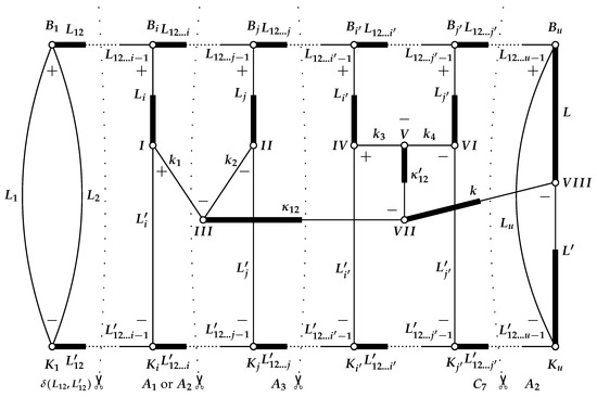
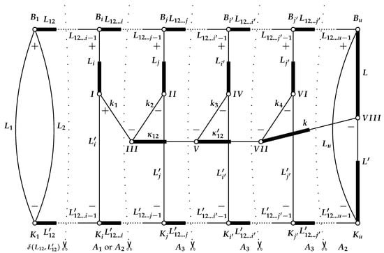
where notation $D^{\left(\lambda \right)}$ denotes the operator of creation or annihilation acting on shell $\lambda$. In addition, the relationship a < b < c < d applies to the expression (18). This means that operator $D^{\left({\lambda }_a\right)}$ acts on shell a, which is in the configuration farthest to the right of shells b, c, and d, etc. Thus, when calculating the reduced matrix element of a two-particle non-scalar operator between configuration state functions (CSFs) with any number of open shells u, it is necessary to find the recoupling matrix for the tensorial structure (18). Its analytical expression is published in P2. It was obtained primarily by using the Jucys and Bandzaitis’ [17] graphical method, representing it graphically, and then, using the rules of this graphical method, the recoupling matrix was simplified by cutting the diagram over two or three angular momentum lines (similar rules to those used in the Jucys, Levinson, and Vanagas [16] method). This allows us to obtain a series of simpler graphical diagrams, which are usually expressed in terms of 3$nj$-coefficients. As mentioned above, the expression for this recoupling matrix is published in P2 (see Equation (27) from P2).

As an illustration, Figure 1 graphically represents, using the Jucys and Bandzaitis’ [17] angular momentum graphical method, such a recoupling matrix $R\left(l_i,l_j,l_i^{\prime },l_j^{\prime },{\Lambda }_l^{bra},{\Lambda }_l^{ket},{\Gamma }_l\right)$, where the primary tensorial structure of a two-particle non-scalar operator is defined as (18) and is acting on four different shells i, j, $i^{\prime }$, $j^{\prime }$, where i < j < i′ < $j^{\prime }$, and where shell i is the rightmost open shell of the configuration and is $i\ge 3$, shell j is the rightmost of $i^{\prime }$ and $j^{\prime }$, etc. (see Figure 8 from [33]).

Figure 1. Diagram representing the recoupling matrix $R\left(l_i,l_j,l_i^{\prime },l_j^{\prime },{\Lambda }_l^{bra},{\Lambda }_l^{ket},{\Gamma }_l\right)$ from P2 when a two-particle non-scalar operator acts upon four shells.

As shown in Figure 1, the bra CSF function shell coupled scheme is represented by the part of the diagram whose nodes are marked ${\mathit{K}}_{\mathbf{1}}$, …, ${\mathit{K}}_{\mathit{i}}$, …, ${\mathit{K}}_{\mathit{j}}$, …, ${\mathit{K}}_{{\mathit{i}}^{\prime }}$, …, ${\mathit{K}}_{{\mathit{j}}^{\prime }}$, …, ${\mathit{K}}_{\mathit{u}}$. The coupled scheme of the ket CSF functions is illustrated in the diagram, where the nodes are labeled ${\mathit{B}}_{\mathbf{1}}$, …, ${\mathit{B}}_{\mathit{i}}$, …, ${\mathit{B}}_{\mathit{j}}$, …, ${\mathit{B}}_{{\mathit{i}}^{\prime }}$, …, ${\mathit{B}}_{{\mathit{j}}^{\prime }}$, …, ${\mathit{B}}_{\mathit{u}}$. We also see that, for example for the bra CSF function, the value of the orbital angular momentum of the first shell is represented in the diagram by the symbol ${\mathit{L}}_{\mathbf{1}}$, the value of the orbital angular momentum of the second shell is represented by ${\mathit{L}}_{\mathbf{2}}$, and their total angular momentum is denoted as ${\mathit{L}}_{\mathbf{12}}$. The sign + at the vertex ${\mathit{B}}_{\mathbf{1}}$ shows that the coupling is done from ${\mathit{L}}_{\mathbf{1}}$ to ${\mathit{L}}_{\mathbf{2}}$ (counterclockwise in the diagram); meanwhile, the sign − at the vertex ${\mathit{K}}_{\mathbf{1}}$ shows that the coupling is done from ${\mathit{L}}_{\mathbf{1}}$ to ${\mathit{L}}_{\mathbf{2}}$ (clockwise in the diagram). All other shells in the diagram are described in the same way in both the bra and ket CSF functions. Meanwhile, the tensorial structure (18) rank connection scheme is represented by vertices marked $\mathit{I}$, $\mathit{II}$, $\mathit{III}$, $\mathit{IV}$, $\mathit{V}$, $\mathit{VI}$, $\mathit{VII}$ and $\mathit{VIII}$. As we can see, maintaining generality in the diagram, the rank of the first operator $D^{\left({\lambda }_a\right)}$ from (18) is denoted by ${\mathit{k}}_{\mathbf{1}}$, i.e., $l_a\equiv {\mathit{k}}_{\mathbf{1}}$, the rank of the second operator $D^{\left({\lambda }_b\right)}$ is denoted by ${\mathit{k}}_{\mathbf{2}}$, i.e., $l_b\equiv {\mathit{k}}_{\mathbf{2}}$, the rank of the third operator $D^{\left({\lambda }_c\right)}$ is denoted by ${\mathit{k}}_{\mathbf{3}}$, i.e., $l_c\equiv {\mathit{k}}_{\mathbf{3}}$, and the rank of the fourth operator $D^{\left({\lambda }_d\right)}$ is denoted by ${\mathit{k}}_{\mathbf{4}}$, i.e., $l_d\equiv {\mathit{k}}_{\mathbf{4}}$. Ranks ${\mathit{k}}_{\mathbf{1}}$ and ${\mathit{k}}_{\mathbf{2}}$ are combined into the substitute rank ${\kappa }_{\mathbf{12}}$ (the same notation in both expression (18) and Figure 1), and ranks ${\mathit{k}}_{\mathbf{3}}$ and ${\mathit{k}}_{\mathbf{4}}$ are combined into the substitute rank ${\kappa }_{\mathbf{12}}^{\prime }$ (the same notation in both expression (18) and Figure 1). Finally, the ranks ${\kappa }_{\mathbf{12}}$ and ${\kappa }_{\mathbf{12}}^{\prime }$ are combined into the final rank $\mathit{k}$. The analytical expression for the recoupling matrix shown in Figure 1 is given by Formula (27) in P2 (actually, the part of the Formula (27) that describes the case $a\ge 3$). In order to obtain this expression, as mentioned above, it is necessary to use the Jucys and Bandzaitis’ [17] methodology, performing certain actions within its framework:

1.

We begin analyzing and reorganizing the diagram from the first nodes on the left, ${\mathit{B}}_{\mathbf{1}}$ and ${\mathit{K}}_{\mathbf{1}}$. As we can see, these two nodes are connected by two lines of angular momentum, ${\mathit{L}}_{\mathbf{1}}$ and ${\mathit{L}}_{\mathbf{2}}$. Therefore, they can be separated from the rest of the diagram by cutting two momentum lines ${\mathit{L}}_{\mathbf{12}}$ and ${\mathit{L}}_{\mathbf{12}}^{\prime }$, as shown by the vertical dotted line in Figure 1. This separation of nodes ${\mathit{B}}_{\mathbf{1}}$ and ${\mathit{K}}_{\mathbf{1}}$, when cutting through two lines of momentum, leads to a triangular delta $\delta \left(L_{12},L_{12}^{\prime }\right)$ and simplification of the remaining diagram. Overall, cutting out this part of the diagram along two angular momentum lines is possible in various graphical methods and is well described, e.g., in [16,17,34,35,36]. This delta function appears as the first delta function in expression (27) of P2 in the case when $a\ge 3$.

2.

In general, when analyzing the rest of the diagram, starting from the left side of the diagram, there may be more cases where both $\mathit{B}$ and $\mathit{K}$ nodes can be separated (one part of the bra CSF function and the other part of the ket CSF function) by cutting only two lines of angular momentum lines. We do this until it is no longer possible to distinguish between the two nodes of the bra and ket functions in the diagram by cutting them with only two lines. Then we arrive at a point on the diagram where these two nodes can be separated by cutting only three lines. In the diagram shown in Figure 1, this location is represented by nodes ${\mathit{B}}_{\mathit{i}}$ and ${\mathit{K}}_{\mathit{i}}$, and the last cut over two lines was made over the ${\mathit{L}}_{\mathbf{12}\dots \mathit{i}-\mathbf{1}}$ and ${\mathit{L}}_{\mathbf{12}\dots \mathit{i}-\mathbf{1}}^{\prime }$ lines.

Any separation of two nodes from the diagram by cutting through two lines leads to a delta function. These delta functions will appear in the analytical expression as many times as we separate the two nodes from the bra and ket functions by cutting only two lines. All delta functions appearing in this section are presented in expression (27) from P2 as “$\dots \delta \left(L_{12\dots a-1},L_{12\dots a-1}^{\prime }\right)$” because in our case $i\equiv a$.

3.

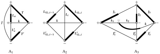
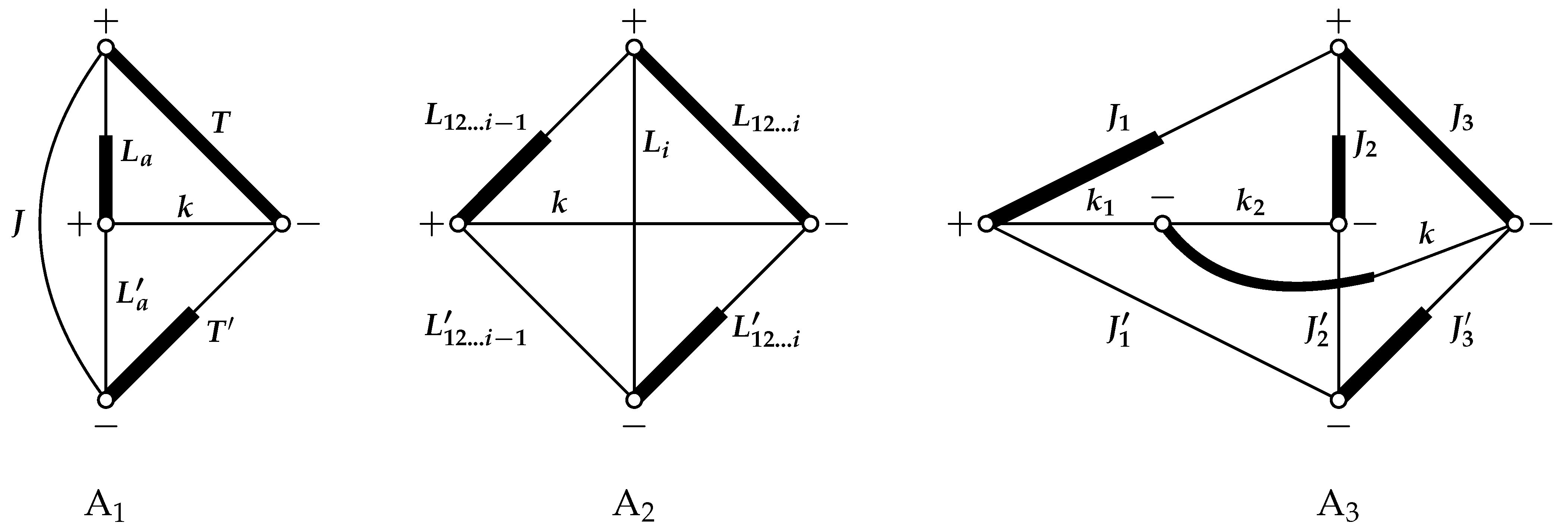
Now we examine the remaining part of the diagram, which includes points ${\mathit{B}}_{\mathit{i}}$, $\mathit{I}$, and ${\mathit{K}}_{\mathit{i}}$. Using the rule of cutting the angular momentum diagram along three lines [16,17,34,35,36,37,38], we can separate these points from the main diagram by cutting along three angular momentum lines ${\mathit{L}}_{\mathbf{12}\dots \mathit{i}}$, ${\mathit{k}}_{\mathbf{1}}$, and ${\mathit{L}}_{\mathbf{12}\dots \mathit{i}}^{\prime }$. This gives us the $A_1$ diagram in Figure 2. This diagram corresponds with the coefficient $C_1$ defined in expression (15) in P2, and its analytical expression is

$$\begin{array}{c}\hfill A_1=C_1={\left(-1\right)}^{\phi }{\left[L_a,T^{\prime }\right]}^{1/2}\left\{\begin{array}{ccc}k& L_a^{\prime }& L_a\\ J& T& T^{\prime }\end{array}\right\},\end{array}$$

(19)

where $a\ge 3$ and the phase factor is $\phi =J+T+L_a^{\prime }+k$.

Figure 2. The angular momentum diagrams that come from the simplification of the recoupling matrix shown in Figure 1 and describe the coefficients $C_1$ and $C_3$ defined in P2 and $C_2$ defined in P3.

This $C_1$ coefficient is in expression (27) when $a\ge 3$ from P2, but it also appears in other cases, including for one, two, and three interacting shells. In all these cases, the values of $\phi$, J, T, and $T^{\prime }$ can be found in Table 2 of P2.

4.

In general, when analyzing the rest of the main diagram, starting from the left side, there may be more cases where cutting along three lines of ${\mathit{L}}_{\mathbf{12}\dots \mathit{m}}$, ${\mathit{k}}_{\mathbf{1}}$, and ${\mathit{L}}_{\mathbf{12}\dots \mathit{m}}$ can separate the nodes ${\mathit{B}}_{\mathit{m}}\dots$ and ${\mathit{K}}_{\mathit{m}}\dots$ belonging to the bra and ket, functions where $i<m>j$ and the node $\mathit{I}$ belong to rank ${\mathit{k}}_{\mathbf{1}}$. Each such cutting of lines produces diagram $A2$ (see Figure 2). This is done until points ${\mathit{B}}_{\mathit{j}}$, $\mathit{II}$, $\mathit{III}$, and ${\mathit{K}}_{\mathit{j}}$ are reached.

Using Jucys and Bandzaitis’ graphical technique [17], we obtain the algebraic expression of diagram $A_2$.

$$\begin{array}{c}\hfill A_2={\left(-1\right)}^{k+L_i+L_{12\dots i-1}+L_{12\dots i}^{\prime }}{\left[L_{12\dots i-1},L_{12\dots i}^{\prime }\right]}^{1/2}\left\{\begin{array}{ccc}k& L_{12\dots i-1}^{\prime }& L_{12\dots i-1}\\ L_i& L_{12\dots i}& L_{12\dots i}^{\prime }\end{array}\right\}.\end{array}$$

(20)

Since, in the most general case, we will have the product of these $A_2$ diagrams, therefore, the coefficient $C_2$ in expression (32) of P3 is expressed through these $A_2$ diagrams as follows:

$$\begin{array}{c}\hfill C_2\left(k,k_{min},k_{max}\right)=\left\{\begin{array}{cc}\begin{array}{c}\hfill {\displaystyle \stackrel{k_{max}}{{\prod }_{i=k_{min}}}{\left(-1\right)}^{k+L_i+L_{12\dots i-1}+L_{12\dots i}^{\prime }}{\left[L_{12\dots i-1},L_{12\dots i}^{\prime }\right]}^{1/2}}\\ \hfill \times \left\{\begin{array}{ccc}k& L_{12\dots i-1}^{\prime }& L_{12\dots i-1}\\ L_i& L_{12\dots i}& L_{12\dots i}^{\prime }\end{array}\right\}\end{array}\hfill & \mathrm{for} k_{min}\le k_{max}\hfill \\ & \\ 0\hfill & \mathrm{for} k_{min}>k_{max}\hfill \end{array}\right.,\end{array}$$

(21)

where $k_{min}$ and $k_{max}$ in our case are $k_{min}=i+1$ and $k_{max}=j-1$. This coefficient also appears in the expression in P2 (27) as $C_2\left(k_1,a+1,b-1\right)$, since $i\equiv a$ and $j\equiv b$. This type of coefficients also appears in other cases of recoupling matrices, including with one, two, and three interacting shells (see P2).

5.

Now we cut nodes ${\mathit{B}}_{\mathit{j}}$, $\mathit{II}$, $\mathit{III}$, and ${\mathit{K}}_{\mathit{j}}$ along three lines ${\mathit{L}}_{\mathbf{12}\dots \mathit{j}}$, ${\kappa }_{\mathbf{12}}$ and ${\mathit{L}}_{\mathbf{12}\dots \mathit{j}}^{\prime }$, thus obtaining diagram $A_3$:

$$\begin{array}{c}\hfill A_3=C_4\left(k_1,k_2,k,P=1\right)={\left[J_1,J_2,J_3^{\prime },k\right]}^{1/2}\left\{\begin{array}{ccc}{J}_1^{\prime }& k_1& J_1\\ J_2^{\prime }& k_2& J_2\\ J_3^{\prime }& k& J_3\end{array}\right\}.\end{array}$$

(22)

As we can see, this diagram is expressed by coefficient $C_4$, which was defined in Formula (21) in P2. This coefficient is also found in expression (27) for the recoupling matrix in the case of four interacting shells in P2. It also appears in other recoupling matrices including with two, and three interacting shells. In all these cases, the values of $J_1$, $J_1^{\prime }$, $J_2$, $J_2^{\prime }$, $J_3$ and $J_3^{\prime }$ are presented in Table 4 of P2.

6.

Now, if possible, we cut out two nodes, one from the bra and one from the ket functions, across the three ${\mathit{L}}_{\mathbf{12}\dots \mathit{m}}$, ${\kappa }_{\mathbf{12}}$, and ${\mathit{L}}_{\mathbf{12}\dots \mathit{m}}^{\prime }$ lines. We do this until we can separate the aforementioned type of nodes from the main diagram by cutting only three lines. Based on the diagram in Figure 1, we have $j<m<i^{\prime }$. In this way, we again obtain the product of $A_2$ diagrams, which corresponds to the coefficient $C_2$, denoted as $C_2\left({\kappa }_{12},b+1,c-1\right)$ in expression (27) of P2, because $j\equiv b$ and $i^{\prime }\equiv c$. If such cutting is impossible, we skip point 6 and proceed to point 7.

7.

Now, the remaining part of our recoupling matrix diagram in Figure 1, on the left, is the most complex. We cut it, as shown in the figure by the vertical dotted line, through the lines ${\mathit{L}}_{\mathbf{12}\dots {\mathit{j}}^{\prime }}$, $\mathit{k}$, and ${\mathit{L}}_{\mathbf{12}\dots {\mathit{j}}^{\prime }}^{\prime }$, separating the nodes ${\mathit{B}}_{{\mathit{i}}^{\prime }}$, $\mathit{IV}$, ${\mathit{K}}_{{\mathit{i}}^{\prime }}$, ${\mathit{B}}_{{\mathit{j}}^{\prime }}$, $\mathit{VI}$, $\mathit{VII}$, and ${\mathit{K}}_{{\mathit{j}}^{\prime }}$ from the rest of the diagram. This part is the most difficult, requiring more efforts to obtain its analytical expression. It is presented in P2 with the newly introduced coefficient $C_7$. As we can see, this coefficient is expressed through various sums of other coefficients, which makes the calculation of this recouping matrix more complex and time-consuming. We will not discuss in detail the further transformations of this part of the recoupling matrix that lead to the expression (28) given in P2, because in this paper, the spin-angular methodology will allow us to avoid this part of the recoupling matrix, and how this is done will be discussed in a further Section 4.2.

8.

Now, if possible, we cut two nodes, one from the bra and one from the ket functions, across the three ${\mathit{L}}_{\mathbf{12}\dots \mathit{m}}$, $\mathit{k}$, and ${\mathit{L}}_{\mathbf{12}\dots \mathit{m}}^{\prime }$ lines. We do this until we reach the nodes ${\mathit{B}}_{\mathit{u}}$ and ${\mathit{K}}_{\mathit{u}}$. Based on the diagram in Figure 1, we have $j^{\prime }<m<u$. In this way, we again obtain the product of the $A_2$ diagrams, which corresponds to the coefficient $C_2$, denoted as $C_2\left(k,d+1,u-1\right)$ in expression (27) of P2, because $j^{\prime }\equiv d$. If such cutting is impossible, we skip point 8 and proceed to point 9.

9.

After completing all of the above actions, we are left with the $A_2$ diagram, which expresses the coefficient $C_3$ with the value given in Formula (17) from P2:

$$\begin{array}{c}\hfill A_2=C_3={\left(-1\right)}^{k+L_i+L_{12\dots i-1}+L_{12\dots i}^{\prime }}{\left[L_{12\dots i-1},L_{12\dots i}^{\prime }\right]}^{1/2}\left\{\begin{array}{ccc}k& L_{12\dots i-1}^{\prime }& L_{12\dots i-1}\\ L_i& L_{12\dots i}& L_{12\dots i}^{\prime }\end{array}\right\},\end{array}$$

(23)

where, in our case (for $a\ge 3$), we need to change the definition from diagram $A_2$ to the definition of coefficient $C_3$ in the following way: $L_i\to j$, $L_{12\dots i}\to T$, $L_{12\dots i}^{\prime }\to T^{\prime }$, $L_{12\dots i-1}\to J$, and $L_{12\dots i-1}^{\prime }\to J^{\prime }$. This type of coefficient also appears in other cases of recoupling matrices, including with one, two, and three interacting shells (see P2). In all these cases, the values of the parameters of this coefficient are given in Table 3 from P2.

So now we have the final analytical expression for the recoupling matrix presented in Figure 1, which was published in P2 (see case $a\ge 3$ in Equation (27)).

4.2. New Analytical Expression for the Recoupling Matrix in the Case of Four Interacting Shells

In this subsection, we present the extension of the spin-angular integration methodology from P2. This is done in the following way: (i) the order of grouping of the second quantization operators remains exactly the same as published in P2, (ii) the tensorial structure is different from the one proposed in P2 and is as follows (differs from (18)):

$$\begin{array}{c}\hfill {\left[{\left[{\left[D^{\left({\lambda }_a\right)}\times D^{\left({\lambda }_b\right)}\right]}^{\left({\kappa }_{12}{\sigma }_{12}\right)}\times D^{\left({\lambda }_c\right)}\right]}^{\left({\kappa }_{12}^{\prime }{\sigma }_{12}^{\prime }\right)}\times D^{\left({\lambda }_d\right)}\right]}^{\left(kk\right)}.\end{array}$$

(24)

The same as for (18), notation $D^{\left(\lambda \right)}$ denotes the operator of creation or annihilation acting on shell $\lambda$. In addition, the relationship a < b < c < d applies to expression (24). This means that operator $D^{\left({\lambda }_a\right)}$ acts on shell a, which is farthest to the right in the configuration of shells b, c, and d, etc. Thus, when calculating the reduced matrix element of a two-particle non-scalar operator between CSF with any number of open shells u, it is also necessary to find the recoupling matrix for the tensorial structure (24).

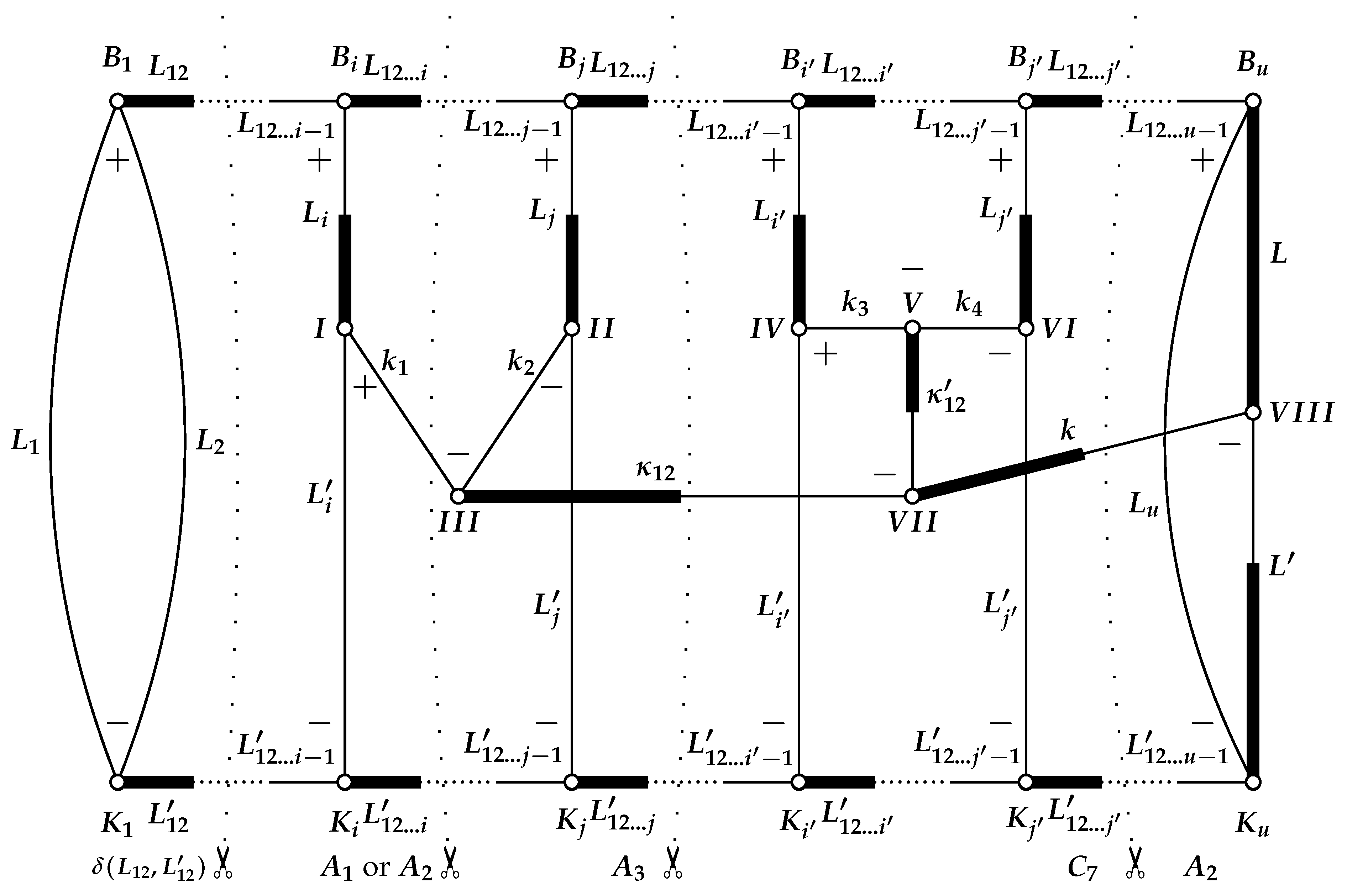
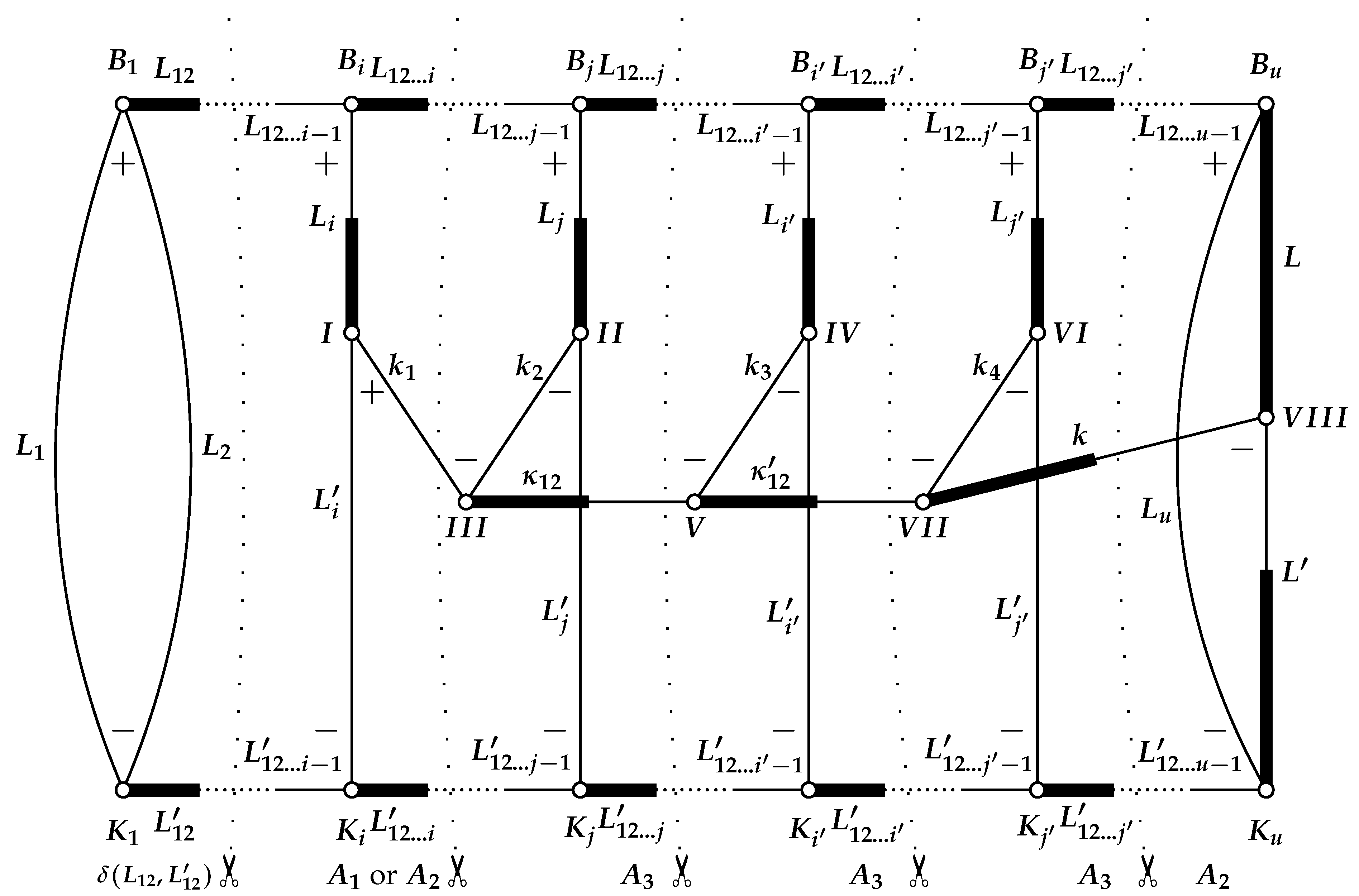
As an illustration, Figure 3 graphically represents, using the Jucys and Bandzaitis’ [17] angular momentum graphical method, such a recoupling matrix $R\left(l_i,l_j,l_i^{\prime },l_j^{\prime },{\Lambda }_l^{bra},{\Lambda }_l^{ket},{\Gamma }_l\right)$, where the primary tensorial structure of a two-particle non-scalar operator is defined as (24) and is acting on four different shells i, j, $i^{\prime }$, $j^{\prime }$, where i < j < i′ < $j^{\prime }$, and where shell i is the rightmost open shell of the configuration and is $i\ge 3$, shell j is the rightmost of $i^{\prime }$ and $j^{\prime }$, etc. As we can see from (24) and Figure 3, the operators are coupled into a tensorial structure sequentially, so the recoupling matrix differs slightly from the previous one from Figure 1. Comparing the previous recoupling matrix (see Figure 1) with the new one (see Figure 3), we see that the part of the diagrams up to points ${\mathit{B}}_{{\mathit{i}}^{\prime }}$, $\mathit{IV}$, and ${\mathit{K}}_{{\mathit{i}}^{\prime }}$ is the same. This means that the parts of the analytical formulas of these recoupling matrices that are to the left of points ${\mathit{B}}_{{\mathit{i}}^{\prime }}$, $\mathit{IV}$, and ${\mathit{K}}_{{\mathit{i}}^{\prime }}$ coincide with each other and are described by diagrams $A_1$, $A_2$, and $A_3$. The difference between these recoupling matrices is that in the new diagram, ranks ${\mathit{\kappa }}_{\mathbf{12}}$ and ${\mathit{k}}_{\mathbf{3}}$ are coupled into rank ${\mathit{\kappa }}_{\mathbf{12}}^{\prime }$, and the latter and rank ${\mathit{k}}_{\mathbf{4}}$ are coupled into the final rank $\mathit{k}$. Meanwhile, in the previous recoupling matrix, ranks ${\mathit{k}}_{\mathbf{3}}$ and ${\mathit{k}}_{\mathbf{4}}$ are coupled into rank ${\mathit{\kappa }}_{\mathbf{12}}^{\prime }$, and rank ${\mathit{\kappa }}_{\mathbf{12}}^{\prime }$ and rank ${\mathit{\kappa }}_{\mathbf{12}}$ are coupled into the final rank $\mathit{k}$. At first glance, the difference does not seem significant, but in fact it is fundamental. This allows us to replace the complex part of the recoupling diagram in Figure 1, which is described by coefficient $C_7$ and whose expression is complicated, with a new part of the diagram which is eventually broken down (by cutting the diagrams only through three angular momentum lines, as shown by the vertical dotted lines in Figure 3) into the combination of $A_2$ and $A_3$ diagrams from Figure 2 we already know, whose algebraic expressions are significantly simpler. The remaining parts of the diagrams in Figure 1 and Figure 3, i.e., the parts from points ${\mathit{K}}_{\mathit{j}}$ and ${\mathit{K}}_{{\mathit{j}}^{\prime }}$ to the right up to the end of the diagrams, are left the same with the same algebraic expressions. This means that the order of operators defined in (24) leads to a significantly simpler expression of the recoupling matrix, which in the most general case, when the operators of second-quantization act upon four shells a, b, c, and d (distributions 19–42 in Table 1 from P2), has the following form:

$$\begin{array}{c}\hfill R\left(l_a,L_a,l_b,L_b,l_c,L_c,l_d,L_d,k_1,k_2,{\kappa }_{12},k_3,k_4,{\kappa }_{12}^{\prime },k\right)\\ \hfill ={\left[L_a,L_b,L_c,L_d\right]}^{-1/2}\delta \left(L_1,L_1^{\prime }\right)\dots \delta \left(L_{a-1},L_{a-1}^{\prime }\right)\delta \left(L_{a+1},L_{a+1}^{\prime }\right)\dots \delta \left(L_{b-1},L_{b-1}^{\prime }\right)\\ \hfill \times \delta \left(L_{b+1},L_{b+1}^{\prime }\right)\dots \delta \left(L_{c-1},L_{c-1}^{\prime }\right)\delta \left(L_{c+1},L_{c+1}^{\prime }\right)\dots \delta \left(L_{d-1},L_{d-1}^{\prime }\right)\delta \left(L_{d+1},L_{d+1}^{\prime }\right)\dots \delta \left(L_u,L_u^{\prime }\right)\\ \hfill \times \left\{\begin{array}{cc}\begin{array}{c}{C}_4\left(k_1,k_2,{\kappa }_{12},1\right)C_2\left({\kappa }_{12},b+1,c-1\right)\hfill \\ \times C_4\left({\kappa }_{12},k_3,k_4,2\right)C_2\left(k_4,c+1,d-1\right)\hfill \\ \times C_4\left(k_4,{\kappa }_{12}^{\prime },k,3\right)C_2\left(k,d+1,u-1\right)C_3;\hfill \end{array}\hfill & \mathrm{for} a=1,b=2\hfill \\ \hfill \\ \begin{array}{c}{C}_1{C}_2\left(k_1,a+1,b-1\right)C_4\left(k_1,k_2,{\kappa }_{12},1\right)\hfill \\ \times C_2\left({\kappa }_{12},b+1,c-1\right)C_4\left({\kappa }_{12},k_3,k_4,2\right)\hfill \\ \times C_2\left(k_4,c+1,d-1\right)C_4\left(k_4,{\kappa }_{12}^{\prime },k,3\right)\hfill \\ \times C_2\left(k,d+1,u-1\right)C_3;\hfill \end{array}\hfill & \mathrm{for} a<3\hfill \\ \hfill \\ \begin{array}{c}\delta \left(L_{12},L_{12}^{\prime }\right)\dots \delta \left(L_{12\dots a-1},L_{12\dots a-1}^{\prime }\right)\hfill \\ \times C_1{C}_2\left(k_1,a+1,b-1\right)C_4\left(k_1,k_2,{\kappa }_{12},1\right)\hfill \\ \times C_2\left({\kappa }_{12},b+1,c-1\right)C_4\left({\kappa }_{12},k_3,k_4,2\right)\hfill \\ \times C_2\left(k_4,c+1,d-1\right)C_4\left(k_4,{\kappa }_{12}^{\prime },k,3\right)\hfill \\ \times C_2\left(k,d+1,u-1\right)C_3;\hfill \end{array}\hfill & \mathrm{for} a\ge 3,\hfill \end{array}\right..\end{array}$$

(25)

When comparing expressions (27) from P2 with (25), we see that the first expression transits to the second expression when we replace the multiplier $C_7(c,d)$ with multipliers $C_4\left({\kappa }_{12},k_3,k_4,2\right)$, $C_2\left(k_4,c+1,d-1\right)$, and $C_4\left(k_4,{\kappa }_{12}^{\prime },k,3\right)$, whose algebraic expressions are simpler and which have already been defined in P2.

Figure 3. Diagram representing the new form (suggested in the current paper) of recoupling matrix $R\left(l_i,l_j,l_i^{\prime },l_j^{\prime },{\Lambda }_l^{bra},{\Lambda }_l^{ket},{\Gamma }_l\right)$ when a two-particle non-scalar operator acts upon four shells.

Coefficients $C_1$, $C_3$, and $C_4$ in (25) are defined the same as in P2 and coefficient $C_2$ is defined the same as in P3, but the values of parameters $\phi$, J, T and $T^{\prime }$ for coefficient $C_1$ are given in Table 1, the values of parameters $\phi$, j, J, $J^{\prime }$, T and $T^{\prime }$ for coefficient $C_3$ are given in Table 2, and the values of parameters $J_1$, $J_1^{\prime }$, $J_2$, $J_2^{\prime }$, $J_3$, and $J_3^{\prime }$ for coefficient $C_4$ must be taken from Table 3 of the current paper. Also, in this case, in the definition of the coefficient $C_1$ given in expression (15) in P2, the variable k should be replaced by the variable $k_1$.

Table 1. Parameters for the coefficient $C_1$ in the case of four interacting shells.

a	$\mathit{\phi }$	J	T	${\mathit{T}}^{\prime }$
1	$L_1+2L_1^{\prime }-L_2-L_{12}^{\prime }+k_1$	$L_2$	$L_{12}$	$L_{12}^{\prime }$
2	$L_1+L_{12}+L_2^{\prime }+k_1$	$L_1$	$L_{12}$	$L_{12}^{\prime }$
$a>2$	$L_{12\dots a-1}+L_{12\dots a}+L_a^{\prime }+k_1$	$L_{12\dots a-1}$	$L_{12\dots a}$	$L_{12\dots a}^{\prime }$

Table 2. Parameters for the coefficient $C_3$ in the case of four interacting shells.

$\mathit{\phi }$	j	J	${\mathit{J}}^{\prime }$	T	${\mathit{T}}^{\prime }$
$k+L_u+L_{12\dots u-1}+L^{\prime }$	$L_u$	$L_{12\dots u-1}$	$L_{12\dots u-1}^{\prime }$	L	$L^{\prime }$

Table 3. Parameters for the coefficient $C_4$ in the case of four interacting shells.

P	a	b	${\mathit{J}}_1$	${\mathit{J}}_1^{\prime }$	${\mathit{J}}_2$	${\mathit{J}}_2^{\prime }$	${\mathit{J}}_3$	${\mathit{J}}_3^{\prime }$
1	1	2	$L_1$	$L_1^{\prime }$	$L_2$	$L_2^{\prime }$	$L_{12}$	$L_{12}$
1	$\ne 1$	$\ne 2$	$L_{1\dots b-1}$	$L_{1\dots b-1}^{\prime }$	$L_b$	$L_b^{\prime }$	$L_{1\dots b}$	$L_{1\dots b}^{\prime }$
2	in all cases		$L_{1\dots c-1}$	$L_{1\dots c-1}^{\prime }$	$L_c$	$L_c^{\prime }$	$L_{1\dots c}$	$L_{1\dots c}^{\prime }$
3	in all cases		$L_{1\dots d-1}$	$L_{1\dots d-1}^{\prime }$	$L_d$	$L_d^{\prime }$	$L_{1\dots d}$	$L_{1\dots d}^{\prime }$

We would like to point out that the main advantage of expression (25) over (27) from P2 is that in expression (25), there are no intermediate sums over parameters $I_1$, $I_2$, and x (see Equations (28), (31) and (32) from P2) related to these summations over 6j-coefficients (see Equations (28)–(32) from P2). This leads to a significantly simpler and faster search for the recoupling matrix $R\left(l_i,l_j,l_i^{\prime },l_j^{\prime },{\Lambda }_l^{bra},{\Lambda }_l^{ket},{\Gamma }_l\right)$, which is crucial for calculating the spin-angular part of a two-particle non-scalar operator.

5. The Amplitude ${\Theta }^{\prime }\left(n_i{\lambda }_i,n_j{\lambda }_j,n_{i^{\prime }}{\lambda }_i^{\prime },n_j^{\prime }{\lambda }_j^{\prime },\Xi \right)$

In this section, we will present new expressions for amplitudes ${\Theta }^{\prime }\left(n_i{\lambda }_i,n_j{\lambda }_j,n_{i^{\prime }}{\lambda }_i^{\prime },n_j^{\prime }{\lambda }_j^{\prime },\Xi \right)$ that are more efficient than those presented in P2. All of them directly flow from the new operator tensorial structure (8) proposed in the current paper. Since the tensorial form of the remaining operators used in P2 and the current paper is the same (see (5)–(7)), only such distributions will be considered where all second quantization operators act on different shells and distributions $\beta \alpha \alpha \alpha$, $\alpha \beta \alpha \alpha$, $\beta \beta \beta \alpha$, and $\beta \beta \alpha \beta$, for which the research managed to obtain simpler algebraic expressions, by using the symmetry properties of the 6j-coefficients and 9j-coefficients, as well as the expression (31.30) by Jucys and Bandzaitis [17] or the expression (9) in Subsection 12.2.2 by Varshalovich, Moskalev and Khersonskii [36]. Since this paper does not examine all distributions, and only part of them, and to make it easier to link the expressions used in the current paper to those presented in P2, the numbering of different cases will be maintained as in P2.

5.1. Two Interacting Shells

5.

Distributions $\beta \alpha \alpha \alpha$, $\alpha \beta \alpha \alpha$ (cases 7, 8 from Table 4):

Table 4. Scheme of the expressions for reduced matrix elements of any non-scalar two-particle operator. The numbers in the table (the first column) correspond to the cases (distributions) discussed in Table 1 of P2.

No.	$\widehat{\mathit{G}}$	$\widehat{\mathit{G}}\left(\mathit{T}\right)$	$\mathit{\alpha }$	$\mathit{\beta }$	$\mathit{\gamma }$	$\mathit{\delta }$	$\tilde{\mathbf{\Theta }}$ or ${\mathbf{\Theta }}^{\prime }$	R	$\mathbf{\Delta }$
1.	Equation (44) [2]	(5)	(14)	–	–	–	Equation (45) [2]	Equation (14) [2]	Equation (41) [2]
	Equation (47) [2]	(5)	(14)	–	–	–	Equation (48) [2],	Equation (14) [2]	Equation (41) [2]
							Equation (49) [2]
2.	Equation (50) [2]	(6)	(11)	(11)	–	–	Equation (51) [2]	Equation (19) [2]	Equation (41) [2]
3.	Equation (50) [2]	(6)	(11)	(11)	–	–	Equation (51) [2]	Equation (19) [2]	Equation (41) [2]
4.	Equation (54) [2]	(6)	(11)	(11)	–	–	Equation (55) [2]	Equation (19) [2]	Equation (41) [2]
5.	Equation (54) [2]	(6)	(11)	(11)	–	–	Equation (55) [2]	Equation (19) [2]	Equation (41) [2]
6.	Equation (52) [2]	(6)	(11)	(11)	–	–	Equation (53) [2]	Equation (19) [2]	Equation (41) [2]
7.	(30)	(6)	(12)	(10)	–	–	(31)	Equation (19) [2]	Equation (42) [2]
8.	(30)	(6)	(12)	(10)	–	–	(32)	Equation (19) [2]	Equation (42) [2]
9.	(36)	(6)	(10)	(13)	–	–	(37)	Equation (19) [2]	Equation (42) [2]
10.	(36)	(6)	(10)	(13)	–	–	(38)	Equation (19) [2]	Equation (42) [2]
11.	Equation (50) [2]	(7)	(10)	(10)	(11)	–	Equation (51) [2]	Equation (24) [2]	Equation (42) [2]
12.	Equation (50) [2]	(7)	(10)	(10)	(11)	–	Equation (51) [2]	Equation (24) [2]	Equation (42) [2]
13.	Equation (54) [2]	(7)	(10)	(10)	(11)	–	Equation (55) [2]	Equation (24) [2]	Equation (42) [2]
14.	Equation (54) [2]	(7)	(10)	(10)	(11)	–	Equation (55) [2]	Equation (24) [2]	Equation (42) [2]
15.	Equation (52) [2]	(7)	(10)	(10)	(11)	–	Equation (53) [2]	Equation (24) [2]	Equation (42) [2]
16.	Equation (52) [2]	(7)	(10)	(10)	(11)	–	Equation (53) [2]	Equation (24) [2]	Equation (42) [2]
17.	Equation (52) [2]	(7)	(10)	(10)	(11)	–	Equation (53) [2]	Equation (24) [2]	Equation (42) [2]
18.	Equation (52) [2]	(7)	(10)	(10)	(11)	–	Equation (53) [2]	Equation (24) [2]	Equation (42) [2]
19.	(39)	(8)	(10)	(10)	(10)	(10)	(40)	(25)	Equation (43) [2]
20.	(39)	(8)	(10)	(10)	(10)	(10)	(41)	(25)	Equation (43) [2]
21.	(39)	(8)	(10)	(10)	(10)	(10)	(42)	(25)	Equation (43) [2]
22.	(39)	(8)	(10)	(10)	(10)	(10)	(43)	(25)	Equation (43) [2]
23.	(44)	(8)	(10)	(10)	(10)	(10)	(45)	(25)	Equation (43) [2]
24.	(44)	(8)	(10)	(10)	(10)	(10)	(46)	(25)	Equation (43) [2]
25.	(44)	(8)	(10)	(10)	(10)	(10)	(47)	(25)	Equation (43) [2]
26.	(44)	(8)	(10)	(10)	(10)	(10)	(48)	(25)	Equation (43) [2]
27.	(49)	(8)	(10)	(10)	(10)	(10)	(50)	(25)	Equation (43) [2]
28.	(51)	(8)	(10)	(10)	(10)	(10)	(52)	(25)	Equation (43) [2]
29.	(54)	(8)	(10)	(10)	(10)	(10)	(55)	(25)	Equation (43) [2]
30.	(51)	(8)	(10)	(10)	(10)	(10)	(53)	(25)	Equation (43) [2]
31.	(56)	(8)	(10)	(10)	(10)	(10)	(57)	(25)	Equation (43) [2]
32.	(58)	(8)	(10)	(10)	(10)	(10)	(59)	(25)	Equation (43) [2]
33.	(60)	(8)	(10)	(10)	(10)	(10)	(62)	(25)	Equation (43) [2]
34.	(60)	(8)	(10)	(10)	(10)	(10)	(61)	(25)	Equation (43) [2]
35.	(63)	(8)	(10)	(10)	(10)	(10)	(64)	(25)	Equation (43) [2]
36.	(65)	(8)	(10)	(10)	(10)	(10)	(66)	(25)	Equation (43) [2]
37.	(67)	(8)	(10)	(10)	(10)	(10)	(68)	(25)	Equation (43) [2]
38.	(67)	(8)	(10)	(10)	(10)	(10)	(69)	(25)	Equation (43) [2]
39.	(70)	(8)	(10)	(10)	(10)	(10)	(71)	(25)	Equation (43) [2]
40.	(72)	(8)	(10)	(10)	(10)	(10)	(73)	(25)	Equation (43) [2]
41.	(74)	(8)	(10)	(10)	(10)	(10)	(75)	(25)	Equation (43) [2]
42.	(74)	(8)	(10)	(10)	(10)	(10)	(76)	(25)	Equation (43) [2]

$$\begin{array}{c}\hfill {\displaystyle \widehat{G}\left(T\right)=\sum _{\begin{array}{c}{\kappa }_{12}{\sigma }_{12}\hfill \\ {\kappa }_{12}^{\prime }{\sigma }_{12}^{\prime }\hfill \end{array}}\sum _{K_l{K}_s}{\Theta }^{\prime }\left(n_i{\lambda }_i,n_j{\lambda }_j,n_i^{\prime }{\lambda }_i^{\prime },n_j^{\prime }{\lambda }_j^{\prime },\Xi \right){\left[a^{\left(l_{\beta }s\right)}\times {\left[a^{\left(l_{\alpha }s\right)}\times {\left[{\tilde{a}}^{\left(l_{\alpha }s\right)}\times {\tilde{a}}^{\left(l_{\alpha }s\right)}\right]}^{\left({\kappa }_{12}^{\prime }{\sigma }_{12}^{\prime }\right)}\right]}^{\left(K_l{K}_s\right)}\right]}_{p,-p}^{\left(kk\right)}.}\end{array}$$

(26)

When $\widehat{G}\left(T\right)=\widehat{G}\left(\beta \alpha \alpha \alpha \right)$, then

$$\begin{array}{c}\hfill {\Theta }^{\prime }\left(n_i{\lambda }_i,n_j{\lambda }_j,n_i^{\prime }{\lambda }_i^{\prime },n_j^{\prime }{\lambda }_j^{\prime },\Xi \right)\equiv \Theta \left(n_{\alpha }{\lambda }_{\alpha },n_{\beta }{\lambda }_{\beta },\Xi \right)\\ \hfill ={\left(-1\right)}^{k-p+{\kappa }_{12}^{\prime }+{\sigma }_{12}^{\prime }+l_{\alpha }+l_{\beta }}{\displaystyle \frac{\left[{\kappa }_{12},{\sigma }_{12}\right]\sqrt{\left[{\kappa }_{12}^{\prime },{\sigma }_{12}^{\prime },K_l,K_s\right]}}{2}}\left(n_{\beta }{\lambda }_{\beta }{n}_{\alpha }{\lambda }_{\alpha }∥g^{\left({\kappa }_1{\kappa }_{2}k,{\sigma }_1{\sigma }_{2}k\right)}∥n_{\alpha }{\lambda }_{\alpha }{n}_{\alpha }{\lambda }_{\alpha }\right)\\ \hfill \times \left\{\begin{array}{ccc}{l}_{\alpha }& l_{\alpha }& {\kappa }_{12}^{\prime }\\ {\kappa }_1& {\kappa }_2& k\\ l_{\beta }& l_{\alpha }& {\kappa }_{12}\end{array}\right\}\left\{\begin{array}{ccc}s& s& {\sigma }_{12}^{\prime }\\ {\sigma }_1& {\sigma }_2& k\\ s& s& {\sigma }_{12}\end{array}\right\}\left\{\begin{array}{ccc}{l}_{\beta }& l_{\alpha }& {\kappa }_{12}\\ {\kappa }_{12}^{\prime }& k& K_l\end{array}\right\}\left\{\begin{array}{ccc}s& s& {\sigma }_{12}\\ {\sigma }_{12}^{\prime }& k& K_s\end{array}\right\},\end{array}$$

(27)

and when $\widehat{G}\left(T\right)=\widehat{G}\left(\alpha \beta \alpha \alpha \right)$, then

$$\begin{array}{c}\hfill {\Theta }^{\prime }\left(n_i{\lambda }_i,n_j{\lambda }_j,n_i^{\prime }{\lambda }_i^{\prime },n_j^{\prime }{\lambda }_j^{\prime },\Xi \right)\equiv \Theta \left(n_{\alpha }{\lambda }_{\alpha },n_{\beta }{\lambda }_{\beta },\Xi \right)\\ \hfill ={\left(-1\right)}^{k-p+{\kappa }_{12}^{\prime }+{\sigma }_{12}^{\prime }+{\kappa }_{12}+{\sigma }_{12}}{\displaystyle \frac{\left[{\kappa }_{12},{\sigma }_{12}\right]\sqrt{\left[{\kappa }_{12}^{\prime },{\sigma }_{12}^{\prime },K_l,K_s\right]}}{2}}\left(n_{\alpha }{\lambda }_{\alpha }{n}_{\beta }{\lambda }_{\beta }∥g^{\left({\kappa }_1{\kappa }_{2}k,{\sigma }_1{\sigma }_{2}k\right)}∥n_{\alpha }{\lambda }_{\alpha }{n}_{\alpha }{\lambda }_{\alpha }\right)\\ \hfill \left\{\begin{array}{ccc}{l}_{\alpha }& l_{\alpha }& {\kappa }_{12}^{\prime }\\ {\kappa }_1& {\kappa }_2& k\\ l_{\alpha }& l_{\beta }& {\kappa }_{12}\end{array}\right\}\left\{\begin{array}{ccc}s& s& {\sigma }_{12}^{\prime }\\ {\sigma }_1& {\sigma }_2& k\\ s& s& {\sigma }_{12}\end{array}\right\}\left\{\begin{array}{ccc}{l}_{\beta }& l_{\alpha }& {\kappa }_{12}\\ {\kappa }_{12}^{\prime }& k& K_l\end{array}\right\}\left\{\begin{array}{ccc}s& s& {\sigma }_{12}\\ {\sigma }_{12}^{\prime }& k& K_s\end{array}\right\}.\end{array}$$

(28)

Expressions (26)–(28) can be simplified by using the symmetry properties of the 6j-coefficients and 9j-coefficients, as well as the expression (31.30) by Jucys and Bandzaitis [17] or the expression (9) in Subsection 12.2.2 by Varshalovich, Moskalev and Khersonskii [36]:

$$\begin{array}{c}\hfill {\displaystyle \sum _x\left[x\right]\left\{\begin{array}{ccc}x& k_2& k_3\\ m& j_1& l_1\end{array}\right\}\left\{\begin{array}{ccc}{j}_1& j_2& j_3\\ l_1& l_2& l_3\\ x& k_2& k_3\end{array}\right\}={\left(-1\right)}^{2m}\left\{\begin{array}{ccc}{j}_1& j_2& j_3\\ l_3& k_3& m\end{array}\right\}\left\{\begin{array}{ccc}{l}_1& l_2& l_3\\ j_2& m& k_2\end{array}\right\}}\end{array}$$

(29)

to obtain the form

$$\begin{array}{c}\hfill {\displaystyle \widehat{G}\left(T\right)=\sum _{{\kappa }_{12}^{\prime }{\sigma }_{12}^{\prime }}\sum _{K_l{K}_s}{\Theta }^{\prime }\left(n_i{\lambda }_i,n_j{\lambda }_j,n_i^{\prime }{\lambda }_i^{\prime },n_j^{\prime }{\lambda }_j^{\prime },\Xi \right){\left[a^{\left(l_{\beta }s\right)}\times {\left[a^{\left(l_{\alpha }s\right)}\times {\left[{\tilde{a}}^{\left(l_{\alpha }s\right)}\times {\tilde{a}}^{\left(l_{\alpha }s\right)}\right]}^{\left({\kappa }_{12}^{\prime }{\sigma }_{12}^{\prime }\right)}\right]}^{\left(K_l{K}_s\right)}\right]}_{p,-p}^{\left(kk\right)},}\end{array}$$

(30)

when $\widehat{G}\left(T\right)=\widehat{G}\left(\beta \alpha \alpha \alpha \right)$, then

$$\begin{array}{c}\hfill {\Theta }^{\prime }\left(n_i{\lambda }_i,n_j{\lambda }_j,n_i^{\prime }{\lambda }_i^{\prime },n_j^{\prime }{\lambda }_j^{\prime },\Xi \right)\equiv \Theta \left(n_{\alpha }{\lambda }_{\alpha },n_{\beta }{\lambda }_{\beta },\Xi \right)\\ \hfill ={\left(-1\right)}^{k-p+{\kappa }_{12}^{\prime }+{\sigma }_{12}^{\prime }+l_{\alpha }+l_{\beta }+2K_l+2K_s}{\displaystyle \frac{\sqrt{\left[{\kappa }_{12}^{\prime },{\sigma }_{12}^{\prime },K_l,K_s\right]}}{2}}\left(n_{\beta }{\lambda }_{\beta }{n}_{\alpha }{\lambda }_{\alpha }∥g^{\left({\kappa }_1{\kappa }_{2}k,{\sigma }_1{\sigma }_{2}k\right)}∥n_{\alpha }{\lambda }_{\alpha }{n}_{\alpha }{\lambda }_{\alpha }\right)\\ \hfill \times \left\{\begin{array}{ccc}{l}_{\alpha }& l_{\alpha }& {\kappa }_{12}^{\prime }\\ l_{\alpha }& K_l& {\kappa }_2\end{array}\right\}\left\{\begin{array}{ccc}{\kappa }_2& {\kappa }_1& k\\ l_{\beta }& K_l& l_{\alpha }\end{array}\right\}\left\{\begin{array}{ccc}s& s& {\sigma }_{12}^{\prime }\\ s& K_s& {\sigma }_2\end{array}\right\}\left\{\begin{array}{ccc}{\sigma }_2& {\sigma }_1& k\\ s& K_s& s\end{array}\right\},\end{array}$$

(31)

and when $\widehat{G}\left(T\right)=\widehat{G}\left(\alpha \beta \alpha \alpha \right)$, then

$$\begin{array}{c}\hfill {\Theta }^{\prime }\left(n_i{\lambda }_i,n_j{\lambda }_j,n_i^{\prime }{\lambda }_i^{\prime },n_j^{\prime }{\lambda }_j^{\prime },\Xi \right)\equiv \Theta \left(n_{\alpha }{\lambda }_{\alpha },n_{\beta }{\lambda }_{\beta },\Xi \right)\\ \hfill ={\left(-1\right)}^{k-p+{\kappa }_1+{\kappa }_2+2{\kappa }_{12}^{\prime }+{\sigma }_1+{\sigma }_2+2{\sigma }_{12}^{\prime }+l_{\alpha }+l_{\beta }+2K_l+2K_s}{\displaystyle \frac{\sqrt{\left[{\kappa }_{12}^{\prime },{\sigma }_{12}^{\prime },K_l,K_s\right]}}{2}}\left(n_{\alpha }{\lambda }_{\alpha }{n}_{\beta }{\lambda }_{\beta }∥g^{\left({\kappa }_1{\kappa }_{2}k,{\sigma }_1{\sigma }_{2}k\right)}∥n_{\alpha }{\lambda }_{\alpha }{n}_{\alpha }{\lambda }_{\alpha }\right)\\ \hfill \times \left\{\begin{array}{ccc}{l}_{\alpha }& l_{\alpha }& {\kappa }_{12}^{\prime }\\ l_{\alpha }& K_l& {\kappa }_1\end{array}\right\}\left\{\begin{array}{ccc}{\kappa }_1& {\kappa }_2& k\\ l_{\beta }& K_l& l_{\alpha }\end{array}\right\}\left\{\begin{array}{ccc}s& s& {\sigma }_{12}^{\prime }\\ s& K_s& {\sigma }_1\end{array}\right\}\left\{\begin{array}{ccc}{\sigma }_1& {\sigma }_2& k\\ s& K_s& s\end{array}\right\}.\end{array}$$

(32)

6.

Distributions $\beta \beta \beta \alpha$ and $\beta \beta \alpha \beta$ (cases 9 and 10 from Table 4):

$$\begin{array}{c}\hfill {\displaystyle \widehat{G}\left(T\right)=\sum _{\begin{array}{c}{\kappa }_{12},{\sigma }_{12}\hfill \\ {\kappa }_{12}^{\prime },{\sigma }_{12}^{\prime }\hfill \end{array}}\sum _{K_l{K}_s}{\Theta }^{\prime }\left(n_i{\lambda }_i,n_j{\lambda }_j,n_i^{\prime }{\lambda }_i^{\prime },n_j^{\prime }{\lambda }_j^{\prime },\Xi \right){\left[{\left[{\left[a^{\left(l_{\beta }s\right)}\times a^{\left(l_{\beta }s\right)}\right]}^{\left({\kappa }_{12}{\sigma }_{12}\right)}\times {\tilde{a}}^{\left(l_{\beta }s\right)}\right]}^{\left(K_l{K}_s\right)}\times {\tilde{a}}^{\left(l_{\alpha }s\right)}\right]}_{p,-p}^{\left(kk\right)}.}\end{array}$$

(33)

When $\widehat{G}\left(T\right)=\widehat{G}\left(\beta \beta \beta \alpha \right)$:

$$\begin{array}{c}\hfill {\Theta }^{\prime }\left(n_i{\lambda }_i,n_j{\lambda }_j,n_i^{\prime }{\lambda }_i^{\prime },n_j^{\prime }{\lambda }_j^{\prime },\Xi \right)\equiv \Theta \left(n_{\alpha }{\lambda }_{\alpha },n_{\beta }{\lambda }_{\beta },\Xi \right)\\ \hfill ={\left(-1\right)}^{k-p+{\kappa }_{12}+{\sigma }_{12}+l_{\alpha }+l_{\beta }}{\displaystyle \frac{\left[{\kappa }_{12}^{\prime },{\sigma }_{12}^{\prime }\right]\sqrt{\left[{\kappa }_{12},{\sigma }_{12},K_l,K_s\right]}}{2}}\left(n_{\beta }{\lambda }_{\beta }{n}_{\beta }{\lambda }_{\beta }∥g^{\left({\kappa }_1{\kappa }_{2}k,{\sigma }_1{\sigma }_{2}k\right)}∥n_{\beta }{\lambda }_{\beta }{n}_{\alpha }{\lambda }_{\alpha }\right)\\ \hfill \times \left\{\begin{array}{ccc}{l}_{\beta }& l_{\alpha }& {\kappa }_{12}^{\prime }\\ {\kappa }_1& {\kappa }_2& k\\ l_{\beta }& l_{\beta }& {\kappa }_{12}\end{array}\right\}\left\{\begin{array}{ccc}s& s& {\sigma }_{12}^{\prime }\\ {\sigma }_1& {\sigma }_2& k\\ s& s& {\sigma }_{12}\end{array}\right\}\left\{\begin{array}{ccc}{l}_{\alpha }& l_{\beta }& {\kappa }_{12}^{\prime }\\ {\kappa }_{12}& k& K_l\end{array}\right\}\left\{\begin{array}{ccc}s& s& {\sigma }_{12}^{\prime }\\ {\sigma }_{12}& k& K_s\end{array}\right\},\end{array}$$

(34)

and when $\widehat{G}\left(T\right)=\widehat{G}\left(\beta \beta \alpha \beta \right)$:

$$\begin{array}{c}\hfill {\Theta }^{\prime }\left(n_i{\lambda }_i,n_j{\lambda }_j,n_i^{\prime }{\lambda }_i^{\prime },n_j^{\prime }{\lambda }_j^{\prime },\Xi \right)\equiv \Theta \left(n_{\alpha }{\lambda }_{\alpha },n_{\beta }{\lambda }_{\beta },\Xi \right)\\ \hfill ={\left(-1\right)}^{k-p+{\kappa }_{12}^{\prime }+{\sigma }_{12}^{\prime }+{\kappa }_{12}+{\sigma }_{12}}{\displaystyle \frac{\left[{\kappa }_{12}^{\prime },{\sigma }_{12}^{\prime }\right]\sqrt{\left[{\kappa }_{12},{\sigma }_{12},K_l,K_s\right]}}{2}}\left(n_{\beta }{\lambda }_{\beta }{n}_{\beta }{\lambda }_{\beta }∥g^{\left({\kappa }_1{\kappa }_{2}k,{\sigma }_1{\sigma }_{2}k\right)}∥n_{\alpha }{\lambda }_{\alpha }{n}_{\beta }{\lambda }_{\beta }\right)\\ \hfill \times \left\{\begin{array}{ccc}{l}_{\alpha }& l_{\beta }& {\kappa }_{12}^{\prime }\\ {\kappa }_1& {\kappa }_2& k\\ l_{\beta }& l_{\beta }& {\kappa }_{12}\end{array}\right\}\left\{\begin{array}{ccc}s& s& {\sigma }_{12}^{\prime }\\ {\sigma }_1& {\sigma }_2& k\\ s& s& {\sigma }_{12}\end{array}\right\}\left\{\begin{array}{ccc}{l}_{\alpha }& l_{\beta }& {\kappa }_{12}^{\prime }\\ {\kappa }_{12}& k& K_l\end{array}\right\}\left\{\begin{array}{ccc}s& s& {\sigma }_{12}^{\prime }\\ {\sigma }_{12}& k& K_s\end{array}\right\}.\end{array}$$

(35)

As above, using (29), the expressions (33)–(35) can be rewritten as follows:

$$\begin{array}{c}\hfill {\displaystyle \widehat{G}\left(T\right)=\sum _{{\kappa }_{12}{\sigma }_{12}}{\Theta }^{\prime }\left(n_i{\lambda }_i,n_j{\lambda }_j,n_i^{\prime }{\lambda }_i^{\prime },n_j^{\prime }{\lambda }_j^{\prime },\Xi \right){\left[{\left[{\left[a^{\left(l_{\beta }s\right)}\times a^{\left(l_{\beta }s\right)}\right]}^{\left({\kappa }_{12}{\sigma }_{12}\right)}\times {\tilde{a}}^{\left(l_{\beta }s\right)}\right]}^{\left(K_l{K}_s\right)}\times {\tilde{a}}^{\left(l_{\alpha }s\right)}\right]}_{p,-p}^{\left(kk\right)},}\end{array}$$

(36)

when $\widehat{G}\left(T\right)=\widehat{G}\left(\beta \beta \beta \alpha \right)$, then

$$\begin{array}{c}\hfill {\Theta }^{\prime }\left(n_i{\lambda }_i,n_j{\lambda }_j,n_i^{\prime }{\lambda }_i^{\prime },n_j^{\prime }{\lambda }_j^{\prime },\Xi \right)\equiv \Theta \left(n_{\alpha }{\lambda }_{\alpha },n_{\beta }{\lambda }_{\beta },\Xi \right)\\ \hfill ={\left(-1\right)}^{k-p+{\kappa }_{12}+{\sigma }_{12}+l_{\alpha }+l_{\beta }+2K_l+2K_s}{\displaystyle \frac{\sqrt{\left[{\kappa }_{12},{\sigma }_{12},K_l,K_s\right]}}{2}}\left(n_{\beta }{\lambda }_{\beta }{n}_{\beta }{\lambda }_{\beta }∥g^{\left({\kappa }_1{\kappa }_{2}k,{\sigma }_1{\sigma }_{2}k\right)}∥n_{\beta }{\lambda }_{\beta }{n}_{\alpha }{\lambda }_{\alpha }\right)\\ \hfill \times \left\{\begin{array}{ccc}{l}_{\beta }& l_{\alpha }& {\kappa }_{12}\\ l_{\beta }& K_l& {\kappa }_1\end{array}\right\}\left\{\begin{array}{ccc}{\kappa }_1& {\kappa }_2& k\\ l_{\alpha }& K_l& l_{\beta }\end{array}\right\}\left\{\begin{array}{ccc}s& s& {\sigma }_{12}\\ s& K_s& {\sigma }_1\end{array}\right\}\left\{\begin{array}{ccc}{\sigma }_1& {\sigma }_2& k\\ s& K_s& s\end{array}\right\},\end{array}$$

(37)

and when $\widehat{G}\left(T\right)=\widehat{G}\left(\beta \beta \alpha \beta \right)$, then

$$\begin{array}{c}\hfill {\Theta }^{\prime }\left(n_i{\lambda }_i,n_j{\lambda }_j,n_i^{\prime }{\lambda }_i^{\prime },n_j^{\prime }{\lambda }_j^{\prime },\Xi \right)\equiv \Theta \left(n_{\alpha }{\lambda }_{\alpha },n_{\beta }{\lambda }_{\beta },\Xi \right)\\ \hfill ={\left(-1\right)}^{k-p+{\kappa }_1+{\kappa }_2+2{\kappa }_{12}+{\sigma }_1+{\sigma }_2+2{\sigma }_{12}+l_{\alpha }+l_{\beta }+2K_l+2K_s}{\displaystyle \frac{\sqrt{\left[{\kappa }_{12},{\sigma }_{12},K_l,K_s\right]}}{2}}\left(n_{\beta }{\lambda }_{\beta }{n}_{\beta }{\lambda }_{\beta }∥g^{\left({\kappa }_1{\kappa }_{2}k,{\sigma }_1{\sigma }_{2}k\right)}∥n_{\alpha }{\lambda }_{\alpha }{n}_{\beta }{\lambda }_{\beta }\right)\\ \hfill \times \left\{\begin{array}{ccc}{l}_{\beta }& l_{\beta }& {\kappa }_{12}\\ l_{\beta }& K_l& {\kappa }_2\end{array}\right\}\left\{\begin{array}{ccc}{\kappa }_2& {\kappa }_1& k\\ l_{\alpha }& K_l& l_{\beta }\end{array}\right\}\left\{\begin{array}{ccc}s& s& {\sigma }_{12}\\ s& K_s& {\sigma }_2\end{array}\right\}\left\{\begin{array}{ccc}{\sigma }_2& {\sigma }_1& k\\ s& K_s& s\end{array}\right\}.\end{array}$$

(38)

5.2. Four Interacting Shells

1.

Distributions $\alpha \beta \gamma \delta$, $\beta \alpha \gamma \delta$, $\alpha \beta \delta \gamma$, and $\beta \alpha \delta \gamma$ (cases 19, 20, 21, and 22 from Table 4):

$$\begin{array}{c}\hfill {\displaystyle \widehat{G}\left(T\right)=\sum _{{\kappa }_{12}{\sigma }_{12}}\sum _{K_l{K}_s}{\Theta }^{\prime }\left(n_i{\lambda }_i,n_j{\lambda }_j,n_i^{\prime }{\lambda }_i^{\prime },n_j^{\prime }{\lambda }_j^{\prime },\Xi \right){\left[{\left[{\left[a^{\left(l_{\alpha }s\right)}\times a^{\left(l_{\beta }s\right)}\right]}^{\left({\kappa }_{12}{\sigma }_{12}\right)}\times {\tilde{a}}^{\left(l_{\gamma }s\right)}\right]}^{\left(K_l{K}_s\right)}\times {\tilde{a}}^{\left(l_{\delta }s\right)}\right]}_{p,-p}^{\left(kk\right)}.}\end{array}$$

(39)

When $\widehat{G}\left(T\right)=\widehat{G}\left(\alpha \beta \gamma \delta \right)$:

$$\begin{array}{c}\hfill {\Theta }^{\prime }\left(n_i{\lambda }_i,n_j{\lambda }_j,n_i^{\prime }{\lambda }_i^{\prime },n_j^{\prime }{\lambda }_j^{\prime },\Xi \right)\equiv \Theta \left(n_{\alpha }{\lambda }_{\alpha },n_{\beta }{\lambda }_{\beta },n_{\gamma }{\lambda }_{\gamma },n_{\delta }{\lambda }_{\delta },\Xi \right)\\ \hfill ={\left(-1\right)}^{k-p+{\kappa }_{12}+{\sigma }_{12}+l_{\gamma }+l_{\delta }+1}{\displaystyle \frac{\sqrt{\left[{\kappa }_{12},{\sigma }_{12},K_l,K_s\right]}}{2}}\left(n_{\alpha }{\lambda }_{\alpha }{n}_{\beta }{\lambda }_{\beta }∥g^{\left({\kappa }_1{\kappa }_{2}k,{\sigma }_1{\sigma }_{2}k\right)}∥n_{\gamma }{\lambda }_{\gamma }{n}_{\delta }{\lambda }_{\delta }\right)\\ \hfill \times \left\{\begin{array}{ccc}{l}_{\beta }& l_{\alpha }& {\kappa }_{12}\\ l_{\gamma }& K_l& {\kappa }_1\end{array}\right\}\left\{\begin{array}{ccc}{\kappa }_1& {\kappa }_2& k\\ l_{\delta }& K_l& l_{\beta }\end{array}\right\}\left\{\begin{array}{ccc}s& s& {\sigma }_{12}\\ s& K_s& {\sigma }_1\end{array}\right\}\left\{\begin{array}{ccc}{\sigma }_1& {\sigma }_2& k\\ s& K_s& s\end{array}\right\},\end{array}$$

(40)

$\widehat{G}\left(T\right)=\widehat{G}\left(\beta \alpha \gamma \delta \right)$:

$$\begin{array}{c}\hfill {\Theta }^{\prime }\left(n_i{\lambda }_i,n_j{\lambda }_j,n_i^{\prime }{\lambda }_i^{\prime },n_j^{\prime }{\lambda }_j^{\prime },\Xi \right)\equiv \Theta \left(n_{\alpha }{\lambda }_{\alpha },n_{\beta }{\lambda }_{\beta },n_{\gamma }{\lambda }_{\gamma },n_{\delta }{\lambda }_{\delta },\Xi \right)\\ \hfill ={\left(-1\right)}^{k-p+l_{\alpha }+l_{\beta }+l_{\gamma }+l_{\delta }+1}{\displaystyle \frac{\sqrt{\left[{\kappa }_{12},{\sigma }_{12},K_l,K_s\right]}}{2}}\left(n_{\beta }{\lambda }_{\beta }{n}_{\alpha }{\lambda }_{\alpha }∥g^{\left({\kappa }_1{\kappa }_{2}k,{\sigma }_1{\sigma }_{2}k\right)}∥n_{\gamma }{\lambda }_{\gamma }{n}_{\delta }{\lambda }_{\delta }\right)\\ \hfill \times \left\{\begin{array}{ccc}{l}_{\alpha }& l_{\beta }& {\kappa }_{12}\\ l_{\gamma }& K_l& {\kappa }_1\end{array}\right\}\left\{\begin{array}{ccc}{\kappa }_1& {\kappa }_2& k\\ l_{\delta }& K_l& l_{\alpha }\end{array}\right\}\left\{\begin{array}{ccc}s& s& {\sigma }_{12}\\ s& K_s& {\sigma }_1\end{array}\right\}\left\{\begin{array}{ccc}{\sigma }_1& {\sigma }_2& k\\ s& K_s& s\end{array}\right\},\end{array}$$

(41)

$\widehat{G}\left(T\right)=\widehat{G}\left(\alpha \beta \delta \gamma \right)$:

$$\begin{array}{c}\hfill {\Theta }^{\prime }\left(n_i{\lambda }_i,n_j{\lambda }_j,n_i^{\prime }{\lambda }_i^{\prime },n_j^{\prime }{\lambda }_j^{\prime },\Xi \right)\equiv \Theta \left(n_{\alpha }{\lambda }_{\alpha },n_{\beta }{\lambda }_{\beta },n_{\gamma }{\lambda }_{\gamma },n_{\delta }{\lambda }_{\delta },\Xi \right)\\ \hfill ={\left(-1\right)}^{k-p+{\kappa }_1+{\kappa }_2+{\sigma }_1+{\sigma }_2+l_{\alpha }+l_{\beta }+l_{\gamma }+l_{\delta }+1}{\displaystyle \frac{\sqrt{\left[{\kappa }_{12},{\sigma }_{12},K_l,K_s\right]}}{2}}\left(n_{\alpha }{\lambda }_{\alpha }{n}_{\beta }{\lambda }_{\beta }∥g^{\left({\kappa }_1{\kappa }_{2}k,{\sigma }_1{\sigma }_{2}k\right)}∥n_{\delta }{\lambda }_{\delta }{n}_{\gamma }{\lambda }_{\gamma }\right)\\ \hfill \times \left\{\begin{array}{ccc}{l}_{\alpha }& l_{\beta }& {\kappa }_{12}\\ l_{\gamma }& K_l& {\kappa }_2\end{array}\right\}\left\{\begin{array}{ccc}{\kappa }_2& {\kappa }_1& k\\ l_{\delta }& K_l& l_{\alpha }\end{array}\right\}\left\{\begin{array}{ccc}s& s& {\sigma }_{12}\\ s& K_s& {\sigma }_2\end{array}\right\}\left\{\begin{array}{ccc}{\sigma }_2& {\sigma }_1& k\\ s& K_s& s\end{array}\right\},\end{array}$$

(42)

and when $\widehat{G}\left(T\right)=\widehat{G}\left(\beta \alpha \delta \gamma \right)$:

$$\begin{array}{c}\hfill {\Theta }^{\prime }\left(n_i{\lambda }_i,n_j{\lambda }_j,n_i^{\prime }{\lambda }_i^{\prime },n_j^{\prime }{\lambda }_j^{\prime },\Xi \right)\equiv \Theta \left(n_{\alpha }{\lambda }_{\alpha },n_{\beta }{\lambda }_{\beta },n_{\gamma }{\lambda }_{\gamma },n_{\delta }{\lambda }_{\delta },\Xi \right)\\ \hfill ={\left(-1\right)}^{k-p+{\kappa }_1+{\kappa }_2+{\kappa }_{12}+{\sigma }_1+{\sigma }_2+{\sigma }_{12}+l_{\gamma }+l_{\delta }+1}{\displaystyle \frac{\sqrt{\left[{\kappa }_{12},{\sigma }_{12},K_l,K_s\right]}}{2}}\left(n_{\beta }{\lambda }_{\beta }{n}_{\alpha }{\lambda }_{\alpha }∥g^{\left({\kappa }_1{\kappa }_{2}k,{\sigma }_1{\sigma }_{2}k\right)}∥n_{\delta }{\lambda }_{\delta }{n}_{\gamma }{\lambda }_{\gamma }\right)\\ \hfill \times \left\{\begin{array}{ccc}{l}_{\beta }& l_{\alpha }& {\kappa }_{12}\\ l_{\gamma }& K_l& {\kappa }_2\end{array}\right\}\left\{\begin{array}{ccc}{\kappa }_2& {\kappa }_1& k\\ l_{\delta }& K_l& l_{\beta }\end{array}\right\}\left\{\begin{array}{ccc}s& s& {\sigma }_{12}\\ s& K_s& {\sigma }_2\end{array}\right\}\left\{\begin{array}{ccc}{\sigma }_2& {\sigma }_1& k\\ s& K_s& s\end{array}\right\}.\end{array}$$

(43)

2.

Distributions $\gamma \delta \alpha \beta$, $\gamma \delta \beta \alpha$, $\delta \gamma \alpha \beta$, and $\delta \gamma \beta \alpha$ (cases 23, 24, 25, and 26 from Table 4):

$$\begin{array}{c}\hfill {\displaystyle \widehat{G}\left(T\right)=\sum _{{\kappa }_{12}{\sigma }_{12}}\sum _{K_l{K}_s}{\Theta }^{\prime }\left(n_i{\lambda }_i,n_j{\lambda }_j,n_i^{\prime }{\lambda }_i^{\prime },n_j^{\prime }{\lambda }_j^{\prime },\Xi \right){\left[{\left[{\left[{\tilde{a}}^{\left(l_{\alpha }s\right)}\times {\tilde{a}}^{\left(l_{\beta }s\right)}\right]}^{\left({\kappa }_{12}{\sigma }_{12}\right)}\times a^{\left(l_{\gamma }s\right)}\right]}^{\left(K_l{K}_s\right)}\times a^{\left(l_{\delta }s\right)}\right]}_{p,-p}^{\left(kk\right)}.}\end{array}$$

(44)

When $\widehat{G}\left(T\right)=\widehat{G}\left(\gamma \delta \alpha \beta \right)$:

$$\begin{array}{c}\hfill {\Theta }^{\prime }\left(n_i{\lambda }_i,n_j{\lambda }_j,n_i^{\prime }{\lambda }_i^{\prime },n_j^{\prime }{\lambda }_j^{\prime },\Xi \right)\equiv \Theta \left(n_{\alpha }{\lambda }_{\alpha },n_{\beta }{\lambda }_{\beta },n_{\gamma }{\lambda }_{\gamma },n_{\delta }{\lambda }_{\delta },\Xi \right)\\ \hfill ={\left(-1\right)}^{k-p+{\kappa }_1+{\kappa }_2+{\kappa }_{12}+{\sigma }_1+{\sigma }_2+{\sigma }_{12}+l_{\alpha }+l_{\beta }+1}{\displaystyle \frac{\sqrt{\left[{\kappa }_{12},{\sigma }_{12},K_l,K_s\right]}}{2}}\left(n_{\gamma }{\lambda }_{\gamma }{n}_{\delta }{\lambda }_{\delta }∥g^{\left({\kappa }_1{\kappa }_{2}k,{\sigma }_1{\sigma }_{2}k\right)}∥n_{\alpha }{\lambda }_{\alpha }{n}_{\beta }{\lambda }_{\beta }\right)\\ \hfill \times \left\{\begin{array}{ccc}{l}_{\beta }& l_{\alpha }& {\kappa }_{12}\\ l_{\gamma }& K_l& {\kappa }_1\end{array}\right\}\left\{\begin{array}{ccc}{\kappa }_1& {\kappa }_2& k\\ l_{\delta }& K_l& l_{\beta }\end{array}\right\}\left\{\begin{array}{ccc}s& s& {\sigma }_{12}\\ s& K_s& {\sigma }_1\end{array}\right\}\left\{\begin{array}{ccc}{\sigma }_1& {\sigma }_2& k\\ s& K_s& s\end{array}\right\},\end{array}$$

(45)

$\widehat{G}\left(T\right)=\widehat{G}\left(\gamma \delta \beta \alpha \right)$:

$$\begin{array}{c}\hfill {\Theta }^{\prime }\left(n_i{\lambda }_i,n_j{\lambda }_j,n_i^{\prime }{\lambda }_i^{\prime },n_j^{\prime }{\lambda }_j^{\prime },\Xi \right)\equiv \Theta \left(n_{\alpha }{\lambda }_{\alpha },n_{\beta }{\lambda }_{\beta },n_{\gamma }{\lambda }_{\gamma },n_{\delta }{\lambda }_{\delta },\Xi \right)\\ \hfill ={\left(-1\right)}^{k-p+{\kappa }_1+{\kappa }_2+{\sigma }_1+{\sigma }_2+1}{\displaystyle \frac{\sqrt{\left[{\kappa }_{12},{\sigma }_{12},K_l,K_s\right]}}{2}}\left(n_{\gamma }{\lambda }_{\gamma }{n}_{\delta }{\lambda }_{\delta }∥g^{\left({\kappa }_1{\kappa }_{2}k,{\sigma }_1{\sigma }_{2}k\right)}∥n_{\beta }{\lambda }_{\beta }{n}_{\alpha }{\lambda }_{\alpha }\right)\\ \hfill \times \left\{\begin{array}{ccc}{l}_{\alpha }& l_{\beta }& {\kappa }_{12}\\ l_{\gamma }& K_l& {\kappa }_1\end{array}\right\}\left\{\begin{array}{ccc}{\kappa }_1& {\kappa }_2& k\\ l_{\delta }& K_l& l_{\alpha }\end{array}\right\}\left\{\begin{array}{ccc}s& s& {\sigma }_{12}\\ s& K_s& {\sigma }_1\end{array}\right\}\left\{\begin{array}{ccc}{\sigma }_1& {\sigma }_2& k\\ s& K_s& s\end{array}\right\},\end{array}$$

(46)

$\widehat{G}\left(T\right)=\widehat{G}\left(\delta \gamma \alpha \beta \right)$:

$$\begin{array}{c}\hfill {\Theta }^{\prime }\left(n_i{\lambda }_i,n_j{\lambda }_j,n_i^{\prime }{\lambda }_i^{\prime },n_j^{\prime }{\lambda }_j^{\prime },\Xi \right)\equiv \Theta \left(n_{\alpha }{\lambda }_{\alpha },n_{\beta }{\lambda }_{\beta },n_{\gamma }{\lambda }_{\gamma },n_{\delta }{\lambda }_{\delta },\Xi \right)\\ \hfill ={\left(-1\right)}^{k-p+1}{\displaystyle \frac{\sqrt{\left[{\kappa }_{12},{\sigma }_{12},K_l,K_s\right]}}{2}}\left(n_{\delta }{\lambda }_{\delta }{n}_{\gamma }{\lambda }_{\gamma }∥g^{\left({\kappa }_1{\kappa }_{2}k,{\sigma }_1{\sigma }_{2}k\right)}∥n_{\alpha }{\lambda }_{\alpha }{n}_{\beta }{\lambda }_{\beta }\right)\\ \hfill \times \left\{\begin{array}{ccc}{l}_{\alpha }& l_{\beta }& {\kappa }_{12}\\ l_{\gamma }& K_l& {\kappa }_2\end{array}\right\}\left\{\begin{array}{ccc}{\kappa }_2& {\kappa }_1& k\\ l_{\delta }& K_l& l_{\alpha }\end{array}\right\}\left\{\begin{array}{ccc}s& s& {\sigma }_{12}\\ s& K_s& {\sigma }_2\end{array}\right\}\left\{\begin{array}{ccc}{\sigma }_2& {\sigma }_1& k\\ s& K_s& s\end{array}\right\},\end{array}$$

(47)

and when $\widehat{G}\left(T\right)=\widehat{G}\left(\delta \gamma \beta \alpha \right)$:

$$\begin{array}{c}\hfill {\Theta }^{\prime }\left(n_i{\lambda }_i,n_j{\lambda }_j,n_i^{\prime }{\lambda }_i^{\prime },n_j^{\prime }{\lambda }_j^{\prime },\Xi \right)\equiv \Theta \left(n_{\alpha }{\lambda }_{\alpha },n_{\beta }{\lambda }_{\beta },n_{\gamma }{\lambda }_{\gamma },n_{\delta }{\lambda }_{\delta },\Xi \right)\\ \hfill ={\left(-1\right)}^{k-p+{\kappa }_{12}+{\sigma }_{12}+l_{\alpha }+l_{\beta }+1}{\displaystyle \frac{\sqrt{\left[{\kappa }_{12},{\sigma }_{12},K_l,K_s\right]}}{2}}\left(n_{\delta }{\lambda }_{\delta }{n}_{\gamma }{\lambda }_{\gamma }∥g^{\left({\kappa }_1{\kappa }_{2}k,{\sigma }_1{\sigma }_{2}k\right)}∥n_{\beta }{\lambda }_{\beta }{n}_{\alpha }{\lambda }_{\alpha }\right)\\ \hfill \times \left\{\begin{array}{ccc}{l}_{\beta }& l_{\alpha }& {\kappa }_{12}\\ l_{\gamma }& K_l& {\kappa }_2\end{array}\right\}\left\{\begin{array}{ccc}{\kappa }_2& {\kappa }_1& k\\ l_{\delta }& K_l& l_{\beta }\end{array}\right\}\left\{\begin{array}{ccc}s& s& {\sigma }_{12}\\ s& K_s& {\sigma }_2\end{array}\right\}\left\{\begin{array}{ccc}{\sigma }_2& {\sigma }_1& k\\ s& K_s& s\end{array}\right\}.\end{array}$$

(48)

3.

Distribution $\alpha \gamma \beta \delta$ (cases 27 from Table 4):

$$\begin{array}{c}\hfill {\displaystyle \widehat{G}\left(T\right)=\sum _{K_l{K}_s}{\Theta }^{\prime }\left(n_i{\lambda }_i,n_j{\lambda }_j,n_i^{\prime }{\lambda }_i^{\prime },n_j^{\prime }{\lambda }_j^{\prime },\Xi \right){\left[{\left[{\left[a^{\left(l_{\alpha }s\right)}\times {\tilde{a}}^{\left(l_{\beta }s\right)}\right]}^{\left({\kappa }_1{\sigma }_1\right)}\times a^{\left(l_{\gamma }s\right)}\right]}^{\left(K_l{K}_s\right)}\times {\tilde{a}}^{\left(l_{\delta }s\right)}\right]}_{p,-p}^{\left(kk\right)}.}\end{array}$$

(49)

When $\widehat{G}\left(T\right)=\widehat{G}\left(\alpha \gamma \beta \delta \right)$:

$$\begin{array}{c}\hfill {\Theta }^{\prime }\left(n_i{\lambda }_i,n_j{\lambda }_j,n_i^{\prime }{\lambda }_i^{\prime },n_j^{\prime }{\lambda }_j^{\prime },\Xi \right)\equiv \Theta \left(n_{\alpha }{\lambda }_{\alpha },n_{\beta }{\lambda }_{\beta },n_{\gamma }{\lambda }_{\gamma },n_{\delta }{\lambda }_{\delta },\Xi \right)\\ \hfill ={\left(-1\right)}^{k-p+{\kappa }_1+{\sigma }_1+l_{\gamma }+l_{\delta }+1}{\displaystyle \frac{1}{2}}\sqrt{{\displaystyle \frac{\left[K_l,K_s\right]}{\left[{\kappa }_1,{\sigma }_1\right]}}}\left(n_{\alpha }{\lambda }_{\alpha }{n}_{\gamma }{\lambda }_{\gamma }∥g^{\left({\kappa }_1{\kappa }_{2}k,{\sigma }_1{\sigma }_{2}k\right)}∥n_{\beta }{\lambda }_{\beta }{n}_{\delta }{\lambda }_{\delta }\right)\\ \hfill \times \left\{\begin{array}{ccc}{\kappa }_1& {\kappa }_2& k\\ l_{\delta }& K_l& l_{\gamma }\end{array}\right\}\left\{\begin{array}{ccc}{\sigma }_1& {\sigma }_2& k\\ s& K_s& s\end{array}\right\}.\end{array}$$

(50)

4.

Distributions $\alpha \gamma \delta \beta$ and $\gamma \alpha \beta \delta$ (cases 28 and 30 from Table 4):

$$\begin{array}{c}\hfill {\displaystyle \widehat{G}\left(T\right)=\sum _{{\kappa }_{12}{\sigma }_{12}}\sum _{K_l{K}_s}{\Theta }^{\prime }\left(n_i{\lambda }_i,n_j{\lambda }_j,n_i^{\prime }{\lambda }_i^{\prime },n_j^{\prime }{\lambda }_j^{\prime },\Xi \right){\left[{\left[{\left[a^{\left(l_{\alpha }s\right)}\times {\tilde{a}}^{\left(l_{\beta }s\right)}\right]}^{\left({\kappa }_{12}{\sigma }_{12}\right)}\times a^{\left(l_{\gamma }s\right)}\right]}^{\left(K_l{K}_s\right)}\times {\tilde{a}}^{\left(l_{\delta }s\right)}\right]}_{p,-p}^{\left(kk\right)}.}\end{array}$$

(51)

When $\widehat{G}\left(T\right)=\widehat{G}\left(\alpha \gamma \delta \beta \right)$:

$$\begin{array}{c}\hfill {\Theta }^{\prime }\left(n_i{\lambda }_i,n_j{\lambda }_j,n_i^{\prime }{\lambda }_i^{\prime },n_j^{\prime }{\lambda }_j^{\prime },\Xi \right)\equiv \Theta \left(n_{\alpha }{\lambda }_{\alpha },n_{\beta }{\lambda }_{\beta },n_{\gamma }{\lambda }_{\gamma },n_{\delta }{\lambda }_{\delta },\Xi \right)\\ \hfill ={\left(-1\right)}^{k-p+{\kappa }_1+{\sigma }_1+l_{\alpha }+l_{\delta }+1}{\displaystyle \frac{\sqrt{\left[{\kappa }_{12},{\sigma }_{12},K_l,K_s\right]}}{2}}\left(n_{\alpha }{\lambda }_{\alpha }{n}_{\gamma }{\lambda }_{\gamma }∥g^{\left({\kappa }_1{\kappa }_{2}k,{\sigma }_1{\sigma }_{2}k\right)}∥n_{\delta }{\lambda }_{\delta }{n}_{\beta }{\lambda }_{\beta }\right)\\ \hfill \times \left\{\begin{array}{ccc}{l}_{\alpha }& l_{\beta }& {\kappa }_{12}\\ l_{\gamma }& K_l& {\kappa }_2\end{array}\right\}\left\{\begin{array}{ccc}{\kappa }_2& {\kappa }_1& k\\ l_{\delta }& K_l& l_{\alpha }\end{array}\right\}\left\{\begin{array}{ccc}s& s& {\sigma }_{12}\\ s& K_s& {\sigma }_2\end{array}\right\}\left\{\begin{array}{ccc}{\sigma }_2& {\sigma }_1& k\\ s& K_s& s\end{array}\right\}.\end{array}$$

(52)

When $\widehat{G}\left(T\right)=\widehat{G}\left(\gamma \alpha \beta \delta \right)$:

$$\begin{array}{c}\hfill {\Theta }^{\prime }\left(n_i{\lambda }_i,n_j{\lambda }_j,n_i^{\prime }{\lambda }_i^{\prime },n_j^{\prime }{\lambda }_j^{\prime },\Xi \right)\equiv \Theta \left(n_{\alpha }{\lambda }_{\alpha },n_{\beta }{\lambda }_{\beta },n_{\gamma }{\lambda }_{\gamma },n_{\delta }{\lambda }_{\delta },\Xi \right)\\ \hfill ={\left(-1\right)}^{k-p+{\kappa }_1+{\sigma }_1+l_{\alpha }+l_{\delta }+1}{\displaystyle \frac{\sqrt{\left[{\kappa }_{12},{\sigma }_{12},K_l,K_s\right]}}{2}}\left(n_{\gamma }{\lambda }_{\gamma }{n}_{\alpha }{\lambda }_{\alpha }∥g^{\left({\kappa }_1{\kappa }_{2}k,{\sigma }_1{\sigma }_{2}k\right)}∥n_{\beta }{\lambda }_{\beta }{n}_{\delta }{\lambda }_{\delta }\right)\\ \hfill \times \left\{\begin{array}{ccc}{l}_{\alpha }& l_{\beta }& {\kappa }_{12}\\ l_{\gamma }& K_l& {\kappa }_1\end{array}\right\}\left\{\begin{array}{ccc}{\kappa }_1& {\kappa }_2& k\\ l_{\delta }& K_l& l_{\alpha }\end{array}\right\}\left\{\begin{array}{ccc}s& s& {\sigma }_{12}\\ s& K_s& {\sigma }_1\end{array}\right\}\left\{\begin{array}{ccc}{\sigma }_1& {\sigma }_2& k\\ s& K_s& s\end{array}\right\}.\end{array}$$

(53)

5.

Distribution $\gamma \alpha \delta \beta$ (d) (case 29 from Table 4):

$$\begin{array}{c}\hfill {\displaystyle \widehat{G}\left(T\right)=\sum _{K_l{K}_s}{\Theta }^{\prime }\left(n_i{\lambda }_i,n_j{\lambda }_j,n_i^{\prime }{\lambda }_i^{\prime },n_j^{\prime }{\lambda }_j^{\prime },\Xi \right){\left[{\left[{\left[a^{\left(l_{\alpha }s\right)}\times {\tilde{a}}^{\left(l_{\beta }s\right)}\right]}^{\left({\kappa }_2{\sigma }_2\right)}\times a^{\left(l_{\gamma }s\right)}\right]}^{\left(K_l{K}_s\right)}\times {\tilde{a}}^{\left(l_{\delta }s\right)}\right]}_{p,-p}^{\left(kk\right)}.}\end{array}$$

(54)

When $\widehat{G}\left(T\right)=\widehat{G}\left(\gamma \alpha \delta \beta \right)$:

$$\begin{array}{c}\hfill {\Theta }^{\prime }\left(n_i{\lambda }_i,n_j{\lambda }_j,n_i^{\prime }{\lambda }_i^{\prime },n_j^{\prime }{\lambda }_j^{\prime },\Xi \right)\equiv \Theta \left(n_{\alpha }{\lambda }_{\alpha },n_{\beta }{\lambda }_{\beta },n_{\gamma }{\lambda }_{\gamma },n_{\delta }{\lambda }_{\delta },\Xi \right)\\ \hfill ={\left(-1\right)}^{k-p+{\kappa }_1+{\sigma }_1+l_{\gamma }+l_{\delta }+1}{\displaystyle \frac{1}{2}}\sqrt{{\displaystyle \frac{\left[K_l,K_s\right]}{\left[{\kappa }_2,{\sigma }_2\right]}}}\left(n_{\gamma }{\lambda }_{\gamma }{n}_{\alpha }{\lambda }_{\alpha }∥g^{\left({\kappa }_1{\kappa }_{2}k,{\sigma }_1{\sigma }_{2}k\right)}∥n_{\delta }{\lambda }_{\delta }{n}_{\beta }{\lambda }_{\beta }\right)\\ \hfill \times \left\{\begin{array}{ccc}{\kappa }_2& {\kappa }_1& k\\ l_{\delta }& K_l& l_{\gamma }\end{array}\right\}\left\{\begin{array}{ccc}{\sigma }_2& {\sigma }_1& k\\ s& K_s& s\end{array}\right\}.\end{array}$$

(55)

6.

Distribution $\beta \delta \alpha \gamma$ (case 31 from Table 4):

$$\begin{array}{c}\hfill {\displaystyle \widehat{G}\left(T\right)=\sum _{K_l{K}_s}{\Theta }^{\prime }\left(n_i{\lambda }_i,n_j{\lambda }_j,n_i^{\prime }{\lambda }_i^{\prime },n_j^{\prime }{\lambda }_j^{\prime },\Xi \right){\left[{\left[{\left[{\tilde{a}}^{\left(l_{\alpha }s\right)}\times a^{\left(l_{\beta }s\right)}\right]}^{\left({\kappa }_1{\sigma }_1\right)}\times {\tilde{a}}^{\left(l_{\gamma }s\right)}\right]}^{\left(K_l{K}_s\right)}\times a^{\left(l_{\delta }s\right)}\right]}_{p,-p}^{\left(kk\right)}.}\end{array}$$

(56)

When $\widehat{G}\left(T\right)=\widehat{G}\left(\beta \delta \alpha \gamma \right)$:

$$\begin{array}{c}\hfill {\Theta }^{\prime }\left(n_i{\lambda }_i,n_j{\lambda }_j,n_i^{\prime }{\lambda }_i^{\prime },n_j^{\prime }{\lambda }_j^{\prime },\Xi \right)\equiv \Theta \left(n_{\alpha }{\lambda }_{\alpha },n_{\beta }{\lambda }_{\beta },n_{\gamma }{\lambda }_{\gamma },n_{\delta }{\lambda }_{\delta },\Xi \right)\\ \hfill ={\left(-1\right)}^{k-p+{\kappa }_2+{\sigma }_2+l_{\alpha }+l_{\beta }+1}{\displaystyle \frac{1}{2}}\sqrt{{\displaystyle \frac{\left[K_l,K_s\right]}{\left[{\kappa }_1,{\sigma }_1\right]}}}\left(n_{\beta }{\lambda }_{\beta }{n}_{\delta }{\lambda }_{\delta }∥g^{\left({\kappa }_1{\kappa }_{2}k,{\sigma }_1{\sigma }_{2}k\right)}∥n_{\alpha }{\lambda }_{\alpha }{n}_{\gamma }{\lambda }_{\gamma }\right)\\ \hfill \times \left\{\begin{array}{ccc}{\kappa }_1& {\kappa }_2& k\\ l_{\delta }& K_l& l_{\gamma }\end{array}\right\}\left\{\begin{array}{ccc}{\sigma }_1& {\sigma }_2& k\\ s& K_s& s\end{array}\right\}.\end{array}$$

(57)

7.

Distribution $\delta \beta \gamma \alpha$ (case 32 from Table 4):

$$\begin{array}{c}\hfill {\displaystyle \widehat{G}\left(T\right)=\sum _{K_l{K}_s}{\Theta }^{\prime }\left(n_i{\lambda }_i,n_j{\lambda }_j,n_i^{\prime }{\lambda }_i^{\prime },n_j^{\prime }{\lambda }_j^{\prime },\Xi \right){\left[{\left[{\left[{\tilde{a}}^{\left(l_{\alpha }s\right)}\times a^{\left(l_{\beta }s\right)}\right]}^{\left({\kappa }_2{\sigma }_2\right)}\times {\tilde{a}}^{\left(l_{\gamma }s\right)}\right]}^{\left(K_l{K}_s\right)}\times a^{\left(l_{\delta }s\right)}\right]}_{p,-p}^{\left(kk\right)}.}\end{array}$$

(58)

When $\widehat{G}\left(T\right)=\widehat{G}\left(\delta \beta \gamma \alpha \right)$:

$$\begin{array}{c}\hfill {\Theta }^{\prime }\left(n_i{\lambda }_i,n_j{\lambda }_j,n_i^{\prime }{\lambda }_i^{\prime },n_j^{\prime }{\lambda }_j^{\prime },\Xi \right)\equiv \Theta \left(n_{\alpha }{\lambda }_{\alpha },n_{\beta }{\lambda }_{\beta },n_{\gamma }{\lambda }_{\gamma },n_{\delta }{\lambda }_{\delta },\Xi \right)\\ \hfill ={\left(-1\right)}^{k-p+{\kappa }_2+{\sigma }_2+l_{\alpha }+l_{\beta }+1}{\displaystyle \frac{1}{2}}\sqrt{{\displaystyle \frac{\left[K_l,K_s\right]}{\left[{\kappa }_2,{\sigma }_2\right]}}}\left(n_{\delta }{\lambda }_{\delta }{n}_{\beta }{\lambda }_{\beta }∥g^{\left({\kappa }_1{\kappa }_{2}k,{\sigma }_1{\sigma }_{2}k\right)}∥n_{\gamma }{\lambda }_{\gamma }{n}_{\alpha }{\lambda }_{\alpha }\right)\\ \hfill \times \left\{\begin{array}{ccc}{\kappa }_2& {\kappa }_1& k\\ l_{\delta }& K_l& l_{\gamma }\end{array}\right\}\left\{\begin{array}{ccc}{\sigma }_2& {\sigma }_1& k\\ s& K_s& s\end{array}\right\}.\end{array}$$

(59)

8.

Distributions $\delta \beta \alpha \gamma$ and $\beta \delta \gamma \alpha$ (cases 33 and 34 from Table 4):

$$\begin{array}{c}\hfill {\displaystyle \widehat{G}\left(T\right)=\sum _{{\kappa }_{12}{\sigma }_{12}}\sum _{K_l{K}_s}{\Theta }^{\prime }\left(n_i{\lambda }_i,n_j{\lambda }_j,n_i^{\prime }{\lambda }_i^{\prime },n_j^{\prime }{\lambda }_j^{\prime },\Xi \right){\left[{\left[{\left[{\tilde{a}}^{\left(l_{\alpha }s\right)}\times a^{\left(l_{\beta }s\right)}\right]}^{\left({\kappa }_{12}{\sigma }_{12}\right)}\times {\tilde{a}}^{\left(l_{\gamma }s\right)}\right]}^{\left(K_l{K}_s\right)}\times a^{\left(l_{\delta }s\right)}\right]}_{p,-p}^{\left(kk\right)}.}\end{array}$$

(60)

When $\widehat{G}\left(T\right)=\widehat{G}\left(\delta \beta \alpha \gamma \right)$:

$$\begin{array}{c}\hfill {\Theta }^{\prime }\left(n_i{\lambda }_i,n_j{\lambda }_j,n_i^{\prime }{\lambda }_i^{\prime },n_j^{\prime }{\lambda }_j^{\prime },\Xi \right)\equiv \Theta \left(n_{\alpha }{\lambda }_{\alpha },n_{\beta }{\lambda }_{\beta },n_{\gamma }{\lambda }_{\gamma },n_{\delta }{\lambda }_{\delta },\Xi \right)\\ \hfill ={\left(-1\right)}^{k-p+{\kappa }_2+{\sigma }_2+l_{\beta }+l_{\gamma }+1}{\displaystyle \frac{\sqrt{\left[{\kappa }_{12},{\sigma }_{12},K_l,K_s\right]}}{2}}\left(n_{\delta }{\lambda }_{\delta }{n}_{\beta }{\lambda }_{\beta }∥g^{\left({\kappa }_1{\kappa }_{2}k,{\sigma }_1{\sigma }_{2}k\right)}∥n_{\alpha }{\lambda }_{\alpha }{n}_{\gamma }{\lambda }_{\gamma }\right)\\ \hfill \times \left\{\begin{array}{ccc}{l}_{\alpha }& l_{\beta }& {\kappa }_{12}\\ l_{\gamma }& K_l& {\kappa }_2\end{array}\right\}\left\{\begin{array}{ccc}{\kappa }_2& {\kappa }_1& k\\ l_{\delta }& K_l& l_{\alpha }\end{array}\right\}\left\{\begin{array}{ccc}s& s& {\sigma }_{12}\\ s& K_s& {\sigma }_2\end{array}\right\}\left\{\begin{array}{ccc}{\sigma }_2& {\sigma }_1& k\\ s& K_s& s\end{array}\right\}.\end{array}$$

(61)

When $\widehat{G}\left(T\right)=\widehat{G}\left(\beta \delta \gamma \alpha \right)$:

$$\begin{array}{c}\hfill {\Theta }^{\prime }\left(n_i{\lambda }_i,n_j{\lambda }_j,n_i^{\prime }{\lambda }_i^{\prime },n_j^{\prime }{\lambda }_j^{\prime },\Xi \right)\equiv \Theta \left(n_{\alpha }{\lambda }_{\alpha },n_{\beta }{\lambda }_{\beta },n_{\gamma }{\lambda }_{\gamma },n_{\delta }{\lambda }_{\delta },\Xi \right)\\ \hfill ={\left(-1\right)}^{k-p+{\kappa }_2+{\sigma }_2+l_{\beta }+l_{\gamma }+1}{\displaystyle \frac{\sqrt{\left[{\kappa }_{12},{\sigma }_{12},K_l,K_s\right]}}{2}}\left(n_{\beta }{\lambda }_{\beta }{n}_{\delta }{\lambda }_{\delta }∥g^{\left({\kappa }_1{\kappa }_{2}k,{\sigma }_1{\sigma }_{2}k\right)}∥n_{\gamma }{\lambda }_{\gamma }{n}_{\alpha }{\lambda }_{\alpha }\right)\\ \hfill \times \left\{\begin{array}{ccc}{l}_{\alpha }& l_{\beta }& {\kappa }_{12}\\ l_{\gamma }& K_l& {\kappa }_1\end{array}\right\}\left\{\begin{array}{ccc}{\kappa }_1& {\kappa }_2& k\\ l_{\delta }& K_l& l_{\alpha }\end{array}\right\}\left\{\begin{array}{ccc}s& s& {\sigma }_{12}\\ s& K_s& {\sigma }_1\end{array}\right\}\left\{\begin{array}{ccc}{\sigma }_1& {\sigma }_2& k\\ s& K_s& s\end{array}\right\}.\end{array}$$

(62)

9.

Distribution $\alpha \delta \beta \gamma$ (case 35 from Table 4):

$$\begin{array}{c}\hfill {\displaystyle \widehat{G}\left(T\right)=\sum _{K_l{K}_s}{\Theta }^{\prime }\left(n_i{\lambda }_i,n_j{\lambda }_j,n_i^{\prime }{\lambda }_i^{\prime },n_j^{\prime }{\lambda }_j^{\prime },\Xi \right){\left[{\left[{\left[a^{\left(l_{\alpha }s\right)}\times {\tilde{a}}^{\left(l_{\beta }s\right)}\right]}^{\left({\kappa }_1{\sigma }_1\right)}\times {\tilde{a}}^{\left(l_{\gamma }s\right)}\right]}^{\left(K_l{K}_s\right)}\times a^{\left(l_{\delta }s\right)}\right]}_{p,-p}^{\left(kk\right)}.}\end{array}$$

(63)

When $\widehat{G}\left(T\right)=\widehat{G}\left(\alpha \delta \beta \gamma \right)$:

$$\begin{array}{c}\hfill {\Theta }^{\prime }\left(n_i{\lambda }_i,n_j{\lambda }_j,n_i^{\prime }{\lambda }_i^{\prime },n_j^{\prime }{\lambda }_j^{\prime },\Xi \right)\equiv \Theta \left(n_{\alpha }{\lambda }_{\alpha },n_{\beta }{\lambda }_{\beta },n_{\gamma }{\lambda }_{\gamma },n_{\delta }{\lambda }_{\delta },\Xi \right)\\ \hfill ={\left(-1\right)}^{k-p+{\kappa }_1+{\sigma }_1-{\kappa }_2-{\sigma }_2+1}{\displaystyle \frac{1}{2}}\sqrt{{\displaystyle \frac{\left[K_l,K_s\right]}{\left[{\kappa }_1,{\sigma }_1\right]}}}\left(n_{\alpha }{\lambda }_{\alpha }{n}_{\delta }{\lambda }_{\delta }∥g^{\left({\kappa }_1{\kappa }_{2}k,{\sigma }_1{\sigma }_{2}k\right)}∥n_{\beta }{\lambda }_{\beta }{n}_{\gamma }{\lambda }_{\gamma }\right)\\ \hfill \times \left\{\begin{array}{ccc}{\kappa }_1& {\kappa }_2& k\\ l_{\delta }& K_l& l_{\gamma }\end{array}\right\}\left\{\begin{array}{ccc}{\sigma }_1& {\sigma }_2& k\\ s& K_s& s\end{array}\right\}.\end{array}$$

(64)

10.

Distribution $\delta \alpha \gamma \beta$ (case 36 from Table 4):

$$\begin{array}{c}\hfill {\displaystyle \widehat{G}\left(T\right)=\sum _{K_l{K}_s}{\Theta }^{\prime }\left(n_i{\lambda }_i,n_j{\lambda }_j,n_i^{\prime }{\lambda }_i^{\prime },n_j^{\prime }{\lambda }_j^{\prime },\Xi \right){\left[{\left[{\left[a^{\left(l_{\alpha }s\right)}\times {\tilde{a}}^{\left(l_{\beta }s\right)}\right]}^{\left({\kappa }_2{\sigma }_2\right)}\times {\tilde{a}}^{\left(l_{\gamma }s\right)}\right]}^{\left(K_l{K}_s\right)}\times a^{\left(l_{\delta }s\right)}\right]}_{p,-p}^{\left(kk\right)}.}\end{array}$$

(65)

When $\widehat{G}\left(T\right)=\widehat{G}\left(\delta \alpha \gamma \beta \right)$:

$$\begin{array}{c}\hfill {\Theta }^{\prime }\left(n_i{\lambda }_i,n_j{\lambda }_j,n_i^{\prime }{\lambda }_i^{\prime },n_j^{\prime }{\lambda }_j^{\prime },\Xi \right)\equiv \Theta \left(n_{\alpha }{\lambda }_{\alpha },n_{\beta }{\lambda }_{\beta },n_{\gamma }{\lambda }_{\gamma },n_{\delta }{\lambda }_{\delta },\Xi \right)\\ \hfill ={\left(-1\right)}^{k-p+1}{\displaystyle \frac{1}{2}}\sqrt{{\displaystyle \frac{\left[K_l,K_s\right]}{\left[{\kappa }_2,{\sigma }_2\right]}}}\left(n_{\delta }{\lambda }_{\delta }{n}_{\alpha }{\lambda }_{\alpha }∥g^{\left({\kappa }_1{\kappa }_{2}k,{\sigma }_1{\sigma }_{2}k\right)}∥n_{\gamma }{\lambda }_{\gamma }{n}_{\beta }{\lambda }_{\beta }\right)\\ \hfill \times \left\{\begin{array}{ccc}{\kappa }_2& {\kappa }_1& k\\ l_{\delta }& K_l& l_{\gamma }\end{array}\right\}\left\{\begin{array}{ccc}{\sigma }_2& {\sigma }_1& k\\ s& K_s& s\end{array}\right\}.\end{array}$$

(66)

11.

Distributions $\alpha \delta \gamma \beta$ and $\delta \alpha \beta \gamma$ (cases 37 and 38 from Table 4):

$$\begin{array}{c}\hfill {\displaystyle \widehat{G}\left(T\right)=\sum _{{\kappa }_{12}{\sigma }_{12}}\sum _{K_l{K}_s}{\Theta }^{\prime }\left(n_i{\lambda }_i,n_j{\lambda }_j,n_i^{\prime }{\lambda }_i^{\prime },n_j^{\prime }{\lambda }_j^{\prime },\Xi \right){\left[{\left[{\left[a^{\left(l_{\alpha }s\right)}\times {\tilde{a}}^{\left(l_{\beta }s\right)}\right]}^{\left({\kappa }_{12}{\sigma }_{12}\right)}\times {\tilde{a}}^{\left(l_{\gamma }s\right)}\right]}^{\left(K_l{K}_s\right)}\times a^{\left(l_{\delta }s\right)}\right]}_{p,-p}^{\left(kk\right)}.}\end{array}$$

(67)

When $\widehat{G}\left(T\right)=\widehat{G}\left(\alpha \delta \gamma \beta \right)$:

$$\begin{array}{c}\hfill {\Theta }^{\prime }\left(n_i{\lambda }_i,n_j{\lambda }_j,n_i^{\prime }{\lambda }_i^{\prime },n_j^{\prime }{\lambda }_j^{\prime },\Xi \right)\equiv \Theta \left(n_{\alpha }{\lambda }_{\alpha },n_{\beta }{\lambda }_{\beta },n_{\gamma }{\lambda }_{\gamma },n_{\delta }{\lambda }_{\delta },\Xi \right)\\ \hfill ={\left(-1\right)}^{k-p+{\kappa }_2+{\kappa }_{12}+{\sigma }_2+{\sigma }_{12}+l_{\beta }+l_{\gamma }+1}{\displaystyle \frac{\sqrt{\left[{\kappa }_{12},{\sigma }_{12},K_l,K_s\right]}}{2}}\left(n_{\alpha }{\lambda }_{\alpha }{n}_{\delta }{\lambda }_{\delta }∥g^{\left({\kappa }_1{\kappa }_{2}k,{\sigma }_1{\sigma }_{2}k\right)}∥n_{\gamma }{\lambda }_{\gamma }{n}_{\beta }{\lambda }_{\beta }\right)\\ \hfill \times \left\{\begin{array}{ccc}{l}_{\beta }& l_{\alpha }& {\kappa }_{12}\\ l_{\gamma }& K_l& {\kappa }_1\end{array}\right\}\left\{\begin{array}{ccc}{\kappa }_1& {\kappa }_2& k\\ l_{\delta }& K_l& l_{\beta }\end{array}\right\}\left\{\begin{array}{ccc}s& s& {\sigma }_{12}\\ s& K_s& {\sigma }_1\end{array}\right\}\left\{\begin{array}{ccc}{\sigma }_1& {\sigma }_2& k\\ s& K_s& s\end{array}\right\}.\end{array}$$

(68)

When $\widehat{G}\left(T\right)=\widehat{G}\left(\delta \alpha \beta \gamma \right)$:

$$\begin{array}{c}\hfill {\Theta }^{\prime }\left(n_i{\lambda }_i,n_j{\lambda }_j,n_i^{\prime }{\lambda }_i^{\prime },n_j^{\prime }{\lambda }_j^{\prime },\Xi \right)\equiv \Theta \left(n_{\alpha }{\lambda }_{\alpha },n_{\beta }{\lambda }_{\beta },n_{\gamma }{\lambda }_{\gamma },n_{\delta }{\lambda }_{\delta },\Xi \right)\\ \hfill ={\left(-1\right)}^{k-p+{\kappa }_2+{\kappa }_{12}+{\sigma }_2+{\sigma }_{12}+l_{\beta }+l_{\gamma }+1}{\displaystyle \frac{\sqrt{\left[{\kappa }_{12},{\sigma }_{12},K_l,K_s\right]}}{2}}\left(n_{\delta }{\lambda }_{\delta }{n}_{\alpha }{\lambda }_{\alpha }∥g^{\left({\kappa }_1{\kappa }_{2}k,{\sigma }_1{\sigma }_{2}k\right)}∥n_{\beta }{\lambda }_{\beta }{n}_{\gamma }{\lambda }_{\gamma }\right)\\ \hfill \times \left\{\begin{array}{ccc}{l}_{\beta }& l_{\alpha }& {\kappa }_{12}\\ l_{\gamma }& K_l& {\kappa }_2\end{array}\right\}\left\{\begin{array}{ccc}{\kappa }_2& {\kappa }_1& k\\ l_{\delta }& K_l& l_{\beta }\end{array}\right\}\left\{\begin{array}{ccc}s& s& {\sigma }_{12}\\ s& K_s& {\sigma }_2\end{array}\right\}\left\{\begin{array}{ccc}{\sigma }_2& {\sigma }_1& k\\ s& K_s& s\end{array}\right\}.\end{array}$$

(69)

12.

Distribution $\beta \gamma \alpha \delta$ (case 39 from Table 4):

$$\begin{array}{c}\hfill {\displaystyle \widehat{G}\left(T\right)=\sum _{K_l{K}_s}{\Theta }^{\prime }\left(n_i{\lambda }_i,n_j{\lambda }_j,n_i^{\prime }{\lambda }_i^{\prime },n_j^{\prime }{\lambda }_j^{\prime },\Xi \right){\left[{\left[{\left[{\tilde{a}}^{\left(l_{\alpha }s\right)}\times a^{\left(l_{\beta }s\right)}\right]}^{\left({\kappa }_1{\sigma }_1\right)}\times a^{\left(l_{\gamma }s\right)}\right]}^{\left(K_l{K}_s\right)}\times {\tilde{a}}^{\left(l_{\delta }s\right)}\right]}_{p,-p}^{\left(kk\right)}.}\end{array}$$

(70)

When $\widehat{G}\left(T\right)=\widehat{G}\left(\beta \gamma \alpha \delta \right)$:

$$\begin{array}{c}\hfill {\Theta }^{\prime }\left(n_i{\lambda }_i,n_j{\lambda }_j,n_i^{\prime }{\lambda }_i^{\prime },n_j^{\prime }{\lambda }_j^{\prime },\Xi \right)\equiv \Theta \left(n_{\alpha }{\lambda }_{\alpha },n_{\beta }{\lambda }_{\beta },n_{\gamma }{\lambda }_{\gamma },n_{\delta }{\lambda }_{\delta },\Xi \right)\\ \hfill ={\left(-1\right)}^{k-p+l_{\alpha }+l_{\beta }+l_{\gamma }+l_{\delta }+1}{\displaystyle \frac{1}{2}}\sqrt{{\displaystyle \frac{\left[K_l,K_s\right]}{\left[{\kappa }_1,{\sigma }_1\right]}}}\left(n_{\beta }{\lambda }_{\beta }{n}_{\gamma }{\lambda }_{\gamma }∥g^{\left({\kappa }_1{\kappa }_{2}k,{\sigma }_1{\sigma }_{2}k\right)}∥n_{\alpha }{\lambda }_{\alpha }{n}_{\delta }{\lambda }_{\delta }\right)\\ \hfill \times \left\{\begin{array}{ccc}{\kappa }_1& {\kappa }_2& k\\ l_{\delta }& K_l& l_{\gamma }\end{array}\right\}\left\{\begin{array}{ccc}{\sigma }_1& {\sigma }_2& k\\ s& K_s& s\end{array}\right\}.\end{array}$$

(71)

13.

Distribution $\gamma \beta \delta \alpha$ (case 40 from Table 4):

$$\begin{array}{c}\hfill {\displaystyle \widehat{G}\left(T\right)=\sum _{K_l{K}_s}{\Theta }^{\prime }\left(n_i{\lambda }_i,n_j{\lambda }_j,n_i^{\prime }{\lambda }_i^{\prime },n_j^{\prime }{\lambda }_j^{\prime },\Xi \right){\left[{\left[{\left[{\tilde{a}}^{\left(l_{\alpha }s\right)}\times a^{\left(l_{\beta }s\right)}\right]}^{\left({\kappa }_2{\sigma }_2\right)}\times a^{\left(l_{\gamma }s\right)}\right]}^{\left(K_l{K}_s\right)}\times {\tilde{a}}^{\left(l_{\delta }s\right)}\right]}_{p,-p}^{\left(kk\right)}.}\end{array}$$

(72)

When $\widehat{G}\left(T\right)=\widehat{G}\left(\gamma \beta \delta \alpha \right)$:

$$\begin{array}{c}\hfill {\Theta }^{\prime }\left(n_i{\lambda }_i,n_j{\lambda }_j,n_i^{\prime }{\lambda }_i^{\prime },n_j^{\prime }{\lambda }_j^{\prime },\Xi \right)\equiv \Theta \left(n_{\alpha }{\lambda }_{\alpha },n_{\beta }{\lambda }_{\beta },n_{\gamma }{\lambda }_{\gamma },n_{\delta }{\lambda }_{\delta },\Xi \right)\\ \hfill ={\left(-1\right)}^{k-p+l_{\alpha }+l_{\beta }+l_{\gamma }+l_{\delta }+{\kappa }_1+{\kappa }_2+{\sigma }_1+{\sigma }_2+1}{\displaystyle \frac{1}{2}}\sqrt{{\displaystyle \frac{\left[K_l,K_s\right]}{\left[{\kappa }_2,{\sigma }_2\right]}}}\left(n_{\gamma }{\lambda }_{\gamma }{n}_{\beta }{\lambda }_{\beta }∥g^{\left({\kappa }_1{\kappa }_{2}k,{\sigma }_1{\sigma }_{2}k\right)}∥n_{\delta }{\lambda }_{\delta }{n}_{\alpha }{\lambda }_{\alpha }\right)\\ \hfill \times \left\{\begin{array}{ccc}{\kappa }_2& {\kappa }_1& k\\ l_{\delta }& K_l& l_{\gamma }\end{array}\right\}\left\{\begin{array}{ccc}{\sigma }_2& {\sigma }_1& k\\ s& K_s& s\end{array}\right\}.\end{array}$$

(73)

14.

Distributions $\beta \gamma \delta \alpha$ and $\gamma \beta \alpha \delta$ (cases 41 and 42 from Table 4):

$$\begin{array}{c}\hfill {\displaystyle \widehat{G}\left(T\right)=\sum _{{\kappa }_{12}{\sigma }_{12}}\sum _{K_l{K}_s}{\Theta }^{\prime }\left(n_i{\lambda }_i,n_j{\lambda }_j,n_i^{\prime }{\lambda }_i^{\prime },n_j^{\prime }{\lambda }_j^{\prime },\Xi \right){\left[{\left[{\left[{\tilde{a}}^{\left(l_{\alpha }s\right)}\times a^{\left(l_{\beta }s\right)}\right]}^{\left({\kappa }_{12}{\sigma }_{12}\right)}\times a^{\left(l_{\gamma }s\right)}\right]}^{\left(K_l{K}_s\right)}\times {\tilde{a}}^{\left(l_{\delta }s\right)}\right]}_{p,-p}^{\left(kk\right)}.}\end{array}$$

(74)

When $\widehat{G}\left(T\right)=\widehat{G}\left(\beta \gamma \delta \alpha \right)$:

$$\begin{array}{c}\hfill {\Theta }^{\prime }\left(n_i{\lambda }_i,n_j{\lambda }_j,n_i^{\prime }{\lambda }_i^{\prime },n_j^{\prime }{\lambda }_j^{\prime },\Xi \right)\equiv \Theta \left(n_{\alpha }{\lambda }_{\alpha },n_{\beta }{\lambda }_{\beta },n_{\gamma }{\lambda }_{\gamma },n_{\delta }{\lambda }_{\delta },\Xi \right)\\ \hfill ={\left(-1\right)}^{k-p+{\kappa }_1+{\kappa }_{12}+{\sigma }_1+{\sigma }_{12}+l_{\alpha }+l_{\delta }+1}{\displaystyle \frac{\sqrt{\left[{\kappa }_{12},{\sigma }_{12},K_l,K_s\right]}}{2}}\left(n_{\beta }{\lambda }_{\beta }{n}_{\gamma }{\lambda }_{\gamma }∥g^{\left({\kappa }_1{\kappa }_{2}k,{\sigma }_1{\sigma }_{2}k\right)}∥n_{\delta }{\lambda }_{\delta }{n}_{\alpha }{\lambda }_{\alpha }\right)\\ \hfill \times \left\{\begin{array}{ccc}{l}_{\beta }& l_{\alpha }& {\kappa }_{12}\\ l_{\gamma }& K_l& {\kappa }_2\end{array}\right\}\left\{\begin{array}{ccc}{\kappa }_2& {\kappa }_1& k\\ l_{\delta }& K_l& l_{\beta }\end{array}\right\}\left\{\begin{array}{ccc}s& s& {\sigma }_{12}\\ s& K_s& {\sigma }_2\end{array}\right\}\left\{\begin{array}{ccc}{\sigma }_2& {\sigma }_1& k\\ s& K_s& s\end{array}\right\}.\end{array}$$

(75)

When $\widehat{G}\left(T\right)=\widehat{G}\left(\gamma \beta \alpha \delta \right)$:

$$\begin{array}{c}\hfill {\Theta }^{\prime }\left(n_i{\lambda }_i,n_j{\lambda }_j,n_i^{\prime }{\lambda }_i^{\prime },n_j^{\prime }{\lambda }_j^{\prime },\Xi \right)\equiv \Theta \left(n_{\alpha }{\lambda }_{\alpha },n_{\beta }{\lambda }_{\beta },n_{\gamma }{\lambda }_{\gamma },n_{\delta }{\lambda }_{\delta },\Xi \right)\\ \hfill ={\left(-1\right)}^{k-p+{\kappa }_1+{\kappa }_{12}+{\sigma }_1+{\sigma }_{12}+l_{\alpha }+l_{\delta }+1}{\displaystyle \frac{\sqrt{\left[{\kappa }_{12},{\sigma }_{12},K_l,K_s\right]}}{2}}\left(n_{\gamma }{\lambda }_{\gamma }{n}_{\beta }{\lambda }_{\beta }∥g^{\left({\kappa }_1{\kappa }_{2}k,{\sigma }_1{\sigma }_{2}k\right)}∥n_{\alpha }{\lambda }_{\alpha }{n}_{\delta }{\lambda }_{\delta }\right)\\ \hfill \times \left\{\begin{array}{ccc}{l}_{\beta }& l_{\alpha }& {\kappa }_{12}\\ l_{\gamma }& K_l& {\kappa }_1\end{array}\right\}\left\{\begin{array}{ccc}{\kappa }_1& {\kappa }_2& k\\ l_{\delta }& K_l& l_{\beta }\end{array}\right\}\left\{\begin{array}{ccc}s& s& {\sigma }_{12}\\ s& K_s& {\sigma }_1\end{array}\right\}\left\{\begin{array}{ccc}{\sigma }_1& {\sigma }_2& k\\ s& K_s& s\end{array}\right\}.\end{array}$$

(76)

6. Evaluation of Methodology Efficiency

The methodology presented in this paper is implemented in the Atsp2K [25] package, i.e., in the programs bp_ang, bp_ang_mpi, bpci, bpci_d, and bpci_mpi. To evaluate the efficiency of the modifications presented in the current paper, we ran two tests on the complex case, in which the configuration has four open shells, including d and f shells. The aim was to assess the advantages of the current methodology over the methodology from P2, demonstrating to what extent the program runs faster with the modifications included.

In the first case, the excited Cm I configuration $5f^{7}6d7s7p$ was considered. A CSF list, required for the RCI method, was generated by performing single excitations from the valence electrons $5f$, $6d$, $7p$, and $7s$ to either the valence shells or the excited shells $5g$ and $6f$. Only CSFs with term ³P were generated. In this case, 7361 CSFs were obtained.

In the second case, the excited Cm I configuration $5f^{5}6d^{2}7p^{2}7s$ was considered. A CSF list, required for the RCI method, was generated by performing single excitations from the valence electrons $5f$, $6d$, $7p$, and $7s$ to either the valence shells or the excited shells $5g$ and $6f$. Only CSFs with term ³P were generated. In this case, 39,724 CSFs were obtained.

The program bp_ang was used to determine the time characteristics. It calculated all required integrals and spin-angular coefficients and wrote them to the corresponding files. The total program execution time was measured (including the calculation time for all the above-mentioned functions) only for the calculation of spin-angular coefficients for the spin–other–orbit and spin–spin operators when the operators acted only on four different shells. It is precisely for this case that the methodology from P2 has been modified to develop the methodology presented in the current paper.

A comparison of computation times is presented in Table 5. In the first test case, the program bp_ang from Atsp2K [25], based on the methodology from P2 and its modifications introduced in the current paper, ran for 41 s and was 26.8 times faster than the program bp_ang from Atsp2K_P2 without the modifications. In the second case, the program bp_ang from Atsp2K ran for 11 min and 23 s and was 36.8 times faster than the program bp_ang from Atsp2K_P2. These test cases are rather hypothetical, but in the case of spin-angular integration, they are particularly complex and demonstrate the advantages of the modifications. It is evident that in the second test case, which is more complex than the first, the speed-up has increased. From these tests, it is clear that in real physical computations, when examining complex multivalence atoms and aiming for high accuracy of their characteristics, the modifications proposed in the current paper are important and, in some cases, critical.

Table 5. A speed-up of Atsp2K [25] as compared with unpublished Atsp2K_P2.

Test Case	List of CSF	Running Time of Atsp2K [25] (in mm:ss)	Running Time of Atsp2K_2P (in mm:ss)	Speed-Up
1	7361	00:41	18:21	26.8
2	39,724	11:23	405:34	35.6

In addition, it is important to note that earlier versions of the Atsp package [4,5,10,39] did not allow the calculations we have examined here. The Atsp2K_P2 and Atsp2K package programs, compared to earlier Atsp versions [4,5,10,39], not only significantly speed up calculations but also expand their capabilities, allowing the inclusion of orbit–orbit interactions and the calculation of configurations with any number of electrons in the f shell. Due to the improved performance of the Atsp2K package, a whole series of high-precision theoretical results have been obtained (see, for example, [40,41,42]).

7. Conclusions

The methodology developed in this paper as compared to P2 allows for a simpler analysis of the most complex two-particle operators, such as the spin–other–orbit and spin–spin, and thus the programs written on its basis are faster. This was achieved by replacing the tensorial structure of the two-particle operator acting on four different shells, defined in P2, with a tensorial structure in which the second quantization operators are coupled sequentially. This led to a difference between the recoupling matrix $R\left({\lambda }_i,{\lambda }_j,{\lambda }_i^{\prime },{\lambda }_j^{\prime },{\Lambda }^{bra},{\Lambda }^{ket},\Gamma \right)$ and the analytical expressions of amplitudes ${\Theta }^{\prime }\left(n_i{\lambda }_i,n_j{\lambda }_j,n_{i^{\prime }}{\lambda }_i^{\prime },n_j^{\prime }{\lambda }_j^{\prime },\Xi \right)$. In the expressions of the recoupling matrix in the current paper, from two to four intermediate sums (depending on the specific case) were eliminated. This simplified the expression itself and sped up calculations. Although the expressions of amplitudes were different, they were equivalent in terms of complexity. Meanwhile, the calculation of quantities $T\left(n_i{\lambda }_i,n_j{\lambda }_j,n_i^{\prime }{\lambda }_i^{\prime },n_j^{\prime }{\lambda }_j^{\prime },{\Lambda }^{bra},{\Lambda }^{ket},\Xi ,\Gamma \right)$ and $\Delta$ remained unchanged. This change in no way diminished the advantages of the existing methodology from P2; rather, it made it even more effective.

The revised methodology is also applicable to $jj$-coupling, as it was in P2. Using it for $jj$-coupling, the s space has to be substituted by the j space and the l space has to be removed in the expressions.

References

- Gaigalas, G.; Rudzikas, Z. On the secondly quantized theory of the many-electron atom. J. Phys. B At. Mol. Phys. 1996, 29, 3303–3318. [Google Scholar] [CrossRef] [Scilit]
- Gaigalas, G.; Rudzikas, Z.; Fischer, C.F. An efficient approach for spin-angular integrations in atomic structure calculations. J. Phys. B At. Mol. Phys. 1997, 30, 3747–3771. [Google Scholar] [CrossRef] [Scilit]
- Gaigalas, G.; Rudzikas, Z.; Scharf, O. Hyperfine Structure Operator in the Tensorial Form of Second Quantization. Cent. Eur. J. Phys. 2004, 2, 720–736. [Google Scholar] [CrossRef] [Scilit]
- Fischer, C.F. A general multi-configuration Hartree-Fock program. Comput. Phys. Commun. 1978, 14, 145–153. [Google Scholar] [CrossRef] [Scilit]
- Fischer, C.F. The MCHF atomic-structure package. Comput. Phys. Commun. 1991, 64, 369–398. [Google Scholar] [CrossRef] [Scilit]
- Fischer, C.F. MCHF atomic-structure package: Support libraries and utilities. Comput. Phys. Commun. 1991, 64, 399–405. [Google Scholar] [CrossRef] [Scilit]
- Hibbert, A.; Fischer, C.F. A general program for computing angular integrals of the non-relativistic Hamiltonian with non-orthogonal orbitals. Comput. Phys. Commun. 1991, 64, 417–430. [Google Scholar] [CrossRef] [Scilit]
- Fischer, C.F. A general multi-configuration Hartree-Fock program. Comput. Phys. Commun. 1991, 64, 431–454. [Google Scholar] [CrossRef] [Scilit]
- Fischer, C.F. The Hartree-Fock Method for Atoms. A Numerical Approach; John Wiley and Sons: New York, NY, USA, 1977. [Google Scholar]
- Fischer, C.F.; Brage, T.; Jönsson, P. Computational Atomic Structure: An MCHF Approach; Institute of Physics Publishing: Bristol, PA, USA; Philadelphia, PA, USA, 1997. [Google Scholar] [CrossRef] [Scilit]
- Dyall, K.G.; Grant, I.P.; Johnson, C.T.; Parpia, F.A.; Plummer, E.P. GRASP: A general-purpose relativistic atomic structure program. Comput. Phys. Commun. 1989, 55, 425–456. [Google Scholar] [CrossRef] [Scilit]
- Parpia, F.; Fischer, C.F.; Grant, I. GRASP92: A package for large-scale relativistic atomic structure calculations. Comput. Phys. Commun. 1996, 94, 249–271. [Google Scholar] [CrossRef] [Scilit]
- Jönsson, P.; He, X.; Fischer, C.F.; Grant, I. The grasp2K relativistic atomic structure package. Comput. Phys. Commun. 2007, 177, 597–622. [Google Scholar] [CrossRef] [Scilit]
- Grant, I. Relativistic Atomic Structure. In Atomic, Molecular and Optical Physics Handbook; Drake, G., Ed.; Springer: Berlin/Heidelberg, Germany, 2006; pp. 325–357. [Google Scholar]
- Fischer, C.F.; Gaigalas, G.; Ralchenko, Y. Some corrections to GRASP92. Comput. Phys. Commun. 2006, 175, 738–744. [Google Scholar] [CrossRef] [Scilit]
- Yutsis, A.; Levinson, I.; Vanagas, V. Mathematical Apparatus of the Theory of Angular Momentum; Israel Program for Scientific Translations Ltd.: Jerusalem, Israel, 1962. [Google Scholar]
- Jucys, A.; Bandzaitis, A. Theory of Angular Momentum in Quantum Mechanics; Mokslas: Vilnius, Lithuania, 1977. [Google Scholar]
- Fano, U.; Racah, G. Irreducible Tensorial Sets; Academic Press: Cambridge, MA, USA, 1959. [Google Scholar]
- Judd, B. Second Quantization and Atomic Spectroscopy; The Johns Hopkins Press: Baltimore, MD, USA, 1967. [Google Scholar]
- Rudzikas, Z.; Kaniauskas, J. Quasispin and Isospin in the Theory of the Atom; Mokslas: Vilnius, Lithuania, 1984. [Google Scholar]
- Gaigalas, G.; Kaniauskas, J.; Rudzikas, Z. A Diagrammatic Technique in the Angular Momentum Theory and Second Quantization. Sov. Phys. Collect. 1985, 25, 3–13. [Google Scholar]
- Rudzikas, Z. Theoretical Atomic Spectroscopy; Cambridge Monographs on Atomic, Molecular and Chemical Physics; Cambridge University Press: Cambridge, UK, 1997. [Google Scholar] [CrossRef] [Scilit]
- Gaigalas, G.; Rudzikas, Z.; Fischer, C.F. Reduced coefficients (subcoefficients) of fractional parentage for p-, d-, and f-shells. At. Data Nucl. Data Tables 1998, 70, 1–39. [Google Scholar] [CrossRef] [Scilit]
- Gaigalas, G.; Fritzsche, S.; Rudzikas, Z. Reduced Coefficients of Fractional Parentage and Matrix Elements of the Tensor W(kqkj) in jj-Coupling. At. Data Nucl. Data Tables 2000, 76, 235–269. [Google Scholar] [CrossRef] [Scilit]
- Fischer, C.F.; Tachiev, G.; Gaigalas, G.; Godefroid, M. An MCHF atomic-structure package for large-scale calculations. Comput. Phys. Commun. 2007, 176, 559–579. [Google Scholar] [CrossRef] [Scilit]
- Jönsson, P.; Gaigalas, G.; Bieroń, J.; Fischer, C.F.; Grant, I. New version: Grasp2K relativistic atomic structure package. Comput. Phys. Commun. 2013, 184, 2197. [Google Scholar] [CrossRef] [Scilit]
- Fischer, C.F.; Gaigalas, G.; Jönsson, P.; Bieroń, J. GRASP2018-A Fortran 95 version of the General Relativistic Atomic Structure Package. Comput. Phys. Commun. 2019, 237, 184–187. [Google Scholar] [CrossRef] [Scilit]
- Gaigalas, G. A program library for computing pure spin-angular coefficients for one- and two-particle operators in relativistic atomic theory. Atoms 2022, 10, 129. [Google Scholar] [CrossRef] [Scilit]
- Gaigalas, G. A program library for computing pure spin-angular coefficients for one- and two-particle operators in non-relativistic atomic theory. Atoms 2026. in preparation. [Google Scholar]
- Gaigalas, G.; Rynkun, P.; Kitovienė, L. Second-order Rayleigh-Schrödinger perturbation theory for the GRASP2018 package: Three-particle Feynman diagram contribution to valence-valence correlations. Lith. J. Phys. 2025, 65, 81–106. [Google Scholar] [CrossRef] [Scilit]
- Dirac, P. The Principles of Quantum Mechanics, 4th ed.; Oxford University Press: Oxford, UK, 1978. [Google Scholar]
- Jucys, A.; Savukynas, A. Mathematical Foundations of the Atomic Theory; Mokslas: Vilnius, Lithuania, 1973. [Google Scholar]
- Gaigalas, G. Integration over spin-angular variables in atomic physics. Lith. J. Phys. 1999, 39, 79–105. [Google Scholar]
- Brink, D.; Satchler, G. Angular Momentum; Clarendon Press: Oxford, UK, 1968. [Google Scholar]
- Lindgren, I.; Morrison, J. Atomic Many-Body Theory, 2nd ed.; Springer: Berlin/Heidelberg, Germany, 1986; reprinted 2009. [Google Scholar]
- Varshalovich, D.; Moskalev, A.; Khersonskii, V. Quantum Theory of Angular Momentum; World Scientific: Singapore, 1988. [Google Scholar] [CrossRef] [Scilit]
- El_Baz, E.; Castel, B. Graphical Methods of Spin Algebras in Atomic, Nuclear and Particle Physics; Marcel Dekker, Inc.: New York, NY, USA, 1972. [Google Scholar]
- Balcar, E.; Lovesey, S.W. Introduction to the Graphical Theory of Angular Momentum. Case Studies; Springer: Berlin/Heidelberg, Germany, 2009. [Google Scholar] [CrossRef] [Scilit]
- Fischer, C.F. The MCHF atomic-structure package. Comput. Phys. Commun. 2000, 128, 635–636. [Google Scholar] [CrossRef] [Scilit]
- Fischer, C.F.; Rubin, R. Breit-Pauli energy levels, transition probabilities and lifetimes for 3d5 levels in Fe IV of astrophysical interest. Mon. Not. R. Astr. Soc. 2004, 355, 461–474. [Google Scholar] [CrossRef] [Scilit]
- Fischer, C.F.; Tachiev, G. Breit-Pauli energy levels, lifetimes, and transition probabilities for the beryllium-like to neon-like sequences. At. Data Nucl. Data Tables 2004, 87, 1–184. [Google Scholar] [CrossRef] [Scilit]
- Fischer, C.F.; Tachiev, G.; Rubin, R.; Rodríguez, M. Analusis of Breit-Pauli Transition Probabilities for Lines in O III. Astrophys. J. 2009, 703, 500–506. [Google Scholar] [CrossRef] [Scilit]
Disclaimer/Publisher’s Note: The statements, opinions and data contained in all publications are solely those of the individual author(s) and contributor(s) and not of MDPI and/or the editor(s). MDPI and/or the editor(s) disclaim responsibility for any injury to people or property resulting from any ideas, methods, instructions or products referred to in the content. |
© 2026 by the author. Licensee MDPI, Basel, Switzerland. This article is an open access article distributed under the terms and conditions of the Creative Commons Attribution (CC BY) license.