jj to LSJ Transformation for Configuration State Functions with an Arbitrary Number of Open Shells

Abstract

This paper presents a methodology that allows for calculated energy levels and other atomic characteristics in relativistic atomic theory, i.e., using the $jj$-coupling scheme, to be identified in terms of $LSJ$-coupling characteristics. The paper begins with outlining the general principles for effectively addressing this problem. Furthermore, it provides a general expression that enables such identification when the atomic state function consists of any number of configuration state functions, each with any number of open shells, and explains how this expression was obtained. The methodology developed in this paper has been successfully implemented in the General Relativistic Atomic Structure Package and can be applied to other similar packages.

1. Introduction

Traditionally, atomic energy spectra and other atomic properties are classified using the quantum numbers of the pure-coupling wave functions. If an atomic state function (ASF) is expressed as a linear combination of nearly pure-coupling functions, the quantum numbers of the function with the largest expansion coefficient are usually used. In principle, any valid coupling scheme can be used to represent the wave function in atomic structure calculations. However, the corresponding identification and classification provide insight into the structure of the atom or ion under consideration only when the quantum numbers are close to their exact values, i.e., when the expansion coefficient of the corresponding nearly pure-coupling wave function approaches 1. The search for such a coupling, where the largest expansion coefficient of the ASF is close to 1, is called the search for an optimal coupling scheme, i.e., the optimal coupling problem.

Nevertheless, the most commonly used coupling schemes in atomic theory are $LSJ$ and $jj$. In atomic spectroscopy, the standard $LSJ$ notation is widely used to classify the level structures of atoms or ions. On the other hand, in many cases, calculations may be performed in the relativistic ($jj$-coupling) scheme [1,2,3] to obtain more accurate data that include relativistic effects, although the results are desired in the $LSJ$-coupling scheme. Thus, in atomic theory, in this case, and in the search for an optimal coupling scheme, it is necessary to be able to move from identifying atomic characteristics in the $jj$-coupling to identifying them in the $LSJ$-coupling, which are discussed in this paper.

The research was carried out in close cooperation with Prof. Charlotte Froese Fischer (1929–2024) and Prof. Zenonas Rokus Rudzikas (1940–2011). The aim of this research was (i) to enable the Atsp [4] and Grasp [5,6] software packages to search for the optimal coupling scheme and (ii) to add a program to the Grasp package that would allow for the identification of the results obtained by Grasp [5,6] in the $LSJ$-coupling scheme. This led to the development of the jj2slj [7] and Coupling [8] programs, which are based on the methodology presented in this paper. These two programs are among the few that integrate Atsp [4] and Grasp [5,6] software packages into a single whole.

The present paper is divided into an Introduction, four sections, and Conclusions. Section 2 provides an outline of the general principles used to effectively identify atomic characteristics within the $LSJ$-coupling scheme. Section 3 addresses the transformation from $jj$-coupling to $LSJ$-coupling for configuration state functions with equivalent electrons. Section 4 presents the general expression for transforming from $jj$-coupling to $LSJ$-coupling for configuration state functions with an arbitrary number of open subshells. The implementation of the methodology in programs is discussed in Section 5.

2. General Theory

Two complete orthonormal bases of wave functions, $\left|{\psi }_i\right)$ and $\left|{\phi }_j\right)$, corresponding to the same specific energy spectrum of a multi-electron system and classified according to the quantum numbers of two different coupling schemes, are related by a unitary transformation. If the corresponding transformation matrices can be chosen to be real, the transformation itself will be orthogonal [3]:

$$\begin{array}{c}\hfill \left|{\psi }_i\right)=\sum _j\left({\phi }_j\left|{\psi }_i\right.\right)\left|{\phi }_j\right),\end{array}$$

(1)

$$\begin{array}{c}\hfill \left|{\phi }_j\right)=\sum _i\left({\psi }_i\left|{\phi }_j\right.\right)\left|{\psi }_i\right).\end{array}$$

(2)

Expressions similar to Equations (1) and (2) may also be written for the wave functions $\left|{\mathrm{\Psi }}_i\right)$ and $\left|{\mathrm{\Phi }}_j\right)$ in intermediate coupling. In particular,

$$\begin{array}{c}\hfill \left|{\mathrm{\Psi }}_i\right)=\sum _j{a}_{ij}\left|{\psi }_j\right),\end{array}$$

(3)

$$\begin{array}{c}\hfill \left|{\mathrm{\Phi }}_j\right)=\sum _k{c}_{jk}\left|{\phi }_k\right),\end{array}$$

(4)

where $a_{ij}$ and $c_{jk}$ are the weights of the wave functions in two pure-coupling schemes. If the wave functions in Equations (3) and (4) share the same eigenvalues (this is the case when we consider, in different coupling schemes, the matrix elements of one and the same Hamiltonian), then, taking into account the orthonormality conditions for the wave functions, we arrive at the following relationships between the weights of the wave functions in two pure-coupling schemes:

$$\begin{array}{c}\hfill c_{jk}=\sum _r{a}_{jr}\left({\phi }_k\left|{\psi }_r\right.\right),\end{array}$$

(5)

$$\begin{array}{c}\hfill a_{ij}=\sum _k{c}_{ik}\left({\psi }_j\left|{\phi }_k\right.\right).\end{array}$$

(6)

It follows from Equations (5) and (6) that given the weights of the wave functions in a particular coupling scheme and the transformation matrix $\left({\phi }_k\left|{\psi }_r\right.\right)$ or $\left({\psi }_j\left|{\phi }_k\right.\right)$, we can easily determine them for any other coupling scheme and thereby select the optimal one without diagonalizing the energy matrices for those schemes.

In the case of multiconfiguration Hartree–Fock (MCHF) [9,10], multiconfiguration Dirac–Hartree–Fock (MCDHF) [2], configuration interaction (CI) [10,11], or relativistic configuration interaction (RCI) [2] methods from atomic theory, functions $\left|{\psi }_i\right)$ and $\left|{\phi }_j\right)$ would correspond to the configuration state functions (CSFs) $\left|{\gamma }_i{L}_i{S}_{i}JP\right.〉$ and $\left|{\gamma }_{j}JP\right.〉$, respectively, for example, $\left|{\gamma }_i{L}_i{S}_{i}JP\right.〉$ in $LSJ$-coupling and $\left|{\gamma }_{j}JP\right.〉$ in $jj$-coupling. Meanwhile, functions $\left|{\mathrm{\Psi }}_i\right)$ and $\left|{\mathrm{\Phi }}_i\right)$ would correspond to the atomic state functions (ASFs) ${\left|{\mathrm{\Psi }}_{\tau }\left(J^P\right)\right.〉}_{LS}$ and ${\left|{\mathrm{\Psi }}_{\tau }\left(J^P\right)\right.〉}_{jj}$, respectively, for example, ${\left|{\mathrm{\Psi }}_{\tau }\left(J^P\right)\right.〉}_{LS}$ in $LSJ$-coupling and ${\left|{\mathrm{\Psi }}_{\tau }\left(J^P\right)\right.〉}_{jj}$ in $jj$-coupling. Thus, with the help of transformation matrices $\left({\phi }_j\left|{\psi }_i\right.\right)$ and $\left({\psi }_i\left|{\phi }_j\right.\right)$, we perform the transformation of the CSF from $jj$-coupling to $LSJ$-coupling, and vice versa, and with the help of Equations (5) and (6), we perform the transformation of the ASF from $jj$-coupling to $LSJ$-coupling, and vice versa. The ASF expansion coefficients $a_{ij}$ and $c_{jk}$ from Equations (3) and (4) are obtained from CI, RCI, MCHF, or MCDHF. Therefore, to perform the aforementioned transformation, it is sufficient to know the expressions for the transformation matrices $\left({\phi }_j\left|{\psi }_i\right.\right)$ and $\left({\psi }_i\left|{\phi }_j\right.\right)$.

In the case of atomic wave functions, the transformation matrices $\left({\phi }_j\left|{\psi }_i\right.\right)$ and $\left({\psi }_i\left|{\phi }_j\right.\right)$ consist of two parts: those that change the coupling scheme within the shell of equivalent electrons (usually $LS$-$jj$) and those that change the coupling scheme between shells of equivalent electrons. The expression obtained from the first part depends on the coefficients of fractional parentage (CFP) used to construct the shell wave function (see Section 3). The expression obtained from the second part is expressed through the 3$nj$-coefficients. The general transformation matrices $\left({\phi }_j\left|{\psi }_i\right.\right)$ and $\left({\psi }_i\left|{\phi }_j\right.\right)$ for the configuration with any number of open shells are constructed from the expressions obtained from the aforementioned two parts (see Section 4). It should also be noted that the transformation matrix $\left({\phi }_j\left|{\psi }_i\right.\right)$ from $jj$-coupling to $LSJ$-coupling is identical to the transformation matrix $\left({\psi }_i\left|{\phi }_j\right.\right)$ from $LSJ$-coupling to $jj$-coupling.

3. Transformation from $jj$-Coupling to $LSJ$-Coupling for Equivalent Electrons

In this section, we consider the transformation between $LSJ$-coupling and $jj$-coupling, and vice versa, when a CSF is formed from only a single open shell in terms of $LSJ$-coupling. In this case, the CSF is

$$\begin{array}{c}\hfill \left|\gamma LSJP\right.〉\equiv |l^w\alpha \nu LS\rangle \end{array}$$

(7)

and

$$\begin{array}{c}\hfill \left|\gamma JP\right.〉\equiv |({\stackrel{-}{l}}^{\stackrel{-}{w}}\stackrel{-}{\nu }\stackrel{-}{J},{\stackrel{+}{l}}^{(w-\stackrel{-}{w})}\stackrel{+}{\nu }\stackrel{+}{J})J\rangle .\end{array}$$

(8)

Each non-relativistic l-orbital (except for s) is associated with two relativistic orbitals $\stackrel{\pm }{l}\equiv j=l\pm 1/2$. Therefore, transforming shell $|n{l}^w\alpha LS\rangle$, which is in $LSJ$-coupling, into $jj$-coupling splits it into two subshells $|n{\stackrel{-}{l}}^{\stackrel{-}{w}}\stackrel{-}{\nu }\stackrel{-}{J}\rangle$ and $|n{\stackrel{+}{l}}^{\stackrel{+}{w}}\stackrel{+}{\nu }\stackrel{+}{J}\rangle$:

$$\begin{array}{c}\hfill |n{l}^w\alpha \nu LS\rangle ⟶\left(|n{\stackrel{-}{l}}^{\stackrel{-}{w}}\stackrel{-}{\nu }\stackrel{-}{J}\rangle ,|n{\stackrel{+}{l}}^{\stackrel{+}{w}}\stackrel{+}{\nu }\stackrel{+}{J}\rangle \right),\end{array}$$

(9)

where $w=\stackrel{-}{w}+\stackrel{+}{w}$, with $\stackrel{-}{w}\left(\max \right)=2l$ and $\stackrel{+}{w}\left(\max \right)=2(l+1)$. The transformation between the shells and subshells in $LSJ$-coupling and $jj$-coupling, respectively, can be written according to [12] as

$$\begin{array}{c}\hfill |l^w\alpha \nu LSJ\rangle =\sum _{\stackrel{-}{\nu }\stackrel{-}{J}\stackrel{+}{\nu }\stackrel{+}{J}\stackrel{-}{w}}|({\stackrel{-}{l}}^{\stackrel{-}{w}}\stackrel{-}{\nu }\stackrel{-}{J},{\stackrel{+}{l}}^{(w-\stackrel{-}{w})}\stackrel{+}{\nu }\stackrel{+}{J})J\rangle \langle ({\stackrel{-}{l}}^{\stackrel{-}{w}}\stackrel{-}{\nu }\stackrel{-}{J},{\stackrel{+}{l}}^{(w-\stackrel{-}{w})}\stackrel{+}{\nu }\stackrel{+}{J})J|l^w\alpha \nu LSJ\rangle ,\end{array}$$

(10)

$$\begin{array}{c}\hfill |({\stackrel{-}{l}}^{\stackrel{-}{w}}\stackrel{-}{\nu }\stackrel{-}{J},{\stackrel{+}{l}}^{(w-\stackrel{-}{w})}\stackrel{+}{\nu }\stackrel{+}{J})J\rangle =\sum _{\alpha \nu LS}|l^w\alpha \nu LSJ\rangle \langle l^w\alpha \nu LSJ|l({\stackrel{-}{l}}^{\stackrel{-}{w}}\stackrel{-}{\nu }\stackrel{-}{J},{\stackrel{+}{l}}^{(w-\stackrel{-}{w})}\stackrel{+}{\nu }\stackrel{+}{J})J\rangle ,\end{array}$$

(11)

which, in both cases, includes a summation over all the quantum numbers except n, l, $\stackrel{-}{l}$, and $\stackrel{+}{l}$.

The $LS$-$jj$ transformation matrices for the shell of equal electrons

$$\begin{array}{c}\hfill \langle ({\stackrel{-}{l}}^{\stackrel{-}{w}}\stackrel{-}{\nu }\stackrel{-}{J},{\stackrel{+}{l}}^{(w-\stackrel{-}{w})}\stackrel{+}{\nu }\stackrel{+}{J})J|l^w\alpha \nu LSJ\rangle =\langle l^w\alpha \nu LSJ|({\stackrel{-}{l}}^{\stackrel{-}{w}}\stackrel{-}{\nu }\stackrel{-}{J},{\stackrel{+}{l}}^{(w-\stackrel{-}{w})}\stackrel{+}{\nu }\stackrel{+}{J})J\rangle \end{array}$$

(12)

in Equations (10) and (11) have simple algebraic expressions when the shell in $LS$-coupling is filled with three electrons (see (14) and (16) in [12]). But of course, these algebraic expressions are not sufficient to analyze more complex atomic systems. The $LS$-$jj$ transformation matrices (Equation (12)) for the shell of equal electrons can be found recursively using expression (8) from [12], where the input transformation matrices have the forms (9) and (10) from [12]. It should be noted that expressions (8) in [12] contain two CPF coefficients: one in the $LSJ$-coupling and the other in the $jj$-coupling. Therefore, the values of the $LS$–$jj$ transformation matrices for the shell of equal electrons found are adjusted to this specific set of CFP coefficients (including the definition of the phase system) and are correct only for them. Using these $LS$–$jj$ transformation matrices in calculations based on CFP coefficients defined differently will produce incorrect results. Therefore, although other publications in the literature also include [13,14] $LS$–$jj$ transformation matrices (Equation (12)) for the shell of equal electrons, they are inconsistent with the phase system and CSF coefficient values used by Atsp and Grasp. Furthermore, they are incomplete because they do not include coefficients for the transformation of the $n{f}^w$ shell. Meanwhile, the values of the $LS$–$jj$ transformation matrices published in [12] are complete and consistent with the CFP reported in [12,15].

4. Transformation from $jj$-Coupling to $LSJ$-Coupling for the Configurations with Arbitrary Number of Open Subshells

Now, in this section, we discuss how the CSF transforms from $jj$-coupling to $LSJ$-coupling in the most general case, i.e., when the CSF has u number (any number) of open shells. Since the CSF transformation from $jj$-coupling to $LSJ$-coupling is identical to the transformation from $LSJ$-coupling to $jj$-coupling, for simplicity, we will focus on the latter. In the most general case, the CSF in $LSJ$-coupling can be written as

$$\begin{array}{c}\hfill \left|\gamma LSJP\right.〉\equiv |((((l_1^{w_1}{\alpha }_1{L}_1{S}_1,l_2^{w_2}{\alpha }_2{L}_2{S}_2)L_{12}{S}_{12},l_3^{w_3}{\alpha }_3{L}_3{S}_3)L_{123}{S}_{123})\dots )LSJ\rangle .\end{array}$$

(13)

As we can see from Equation (13), the shells are consistently coupled separately in the l and s spaces into the resulting angular momenta L and S, respectively. These latter momenta are finally coupled into a total angular momentum J. We also see that when angular momenta are coupled, intermediate resulting angular momentum arise. For example, when the angular momentum $L_1$ of the first shell in the l space is coupled with the angular momentum $L_2$ of the second shell, we obtain an intermediate angular momentum $L_{12}$. The same thing happens when other shells are coupled in both l and s spaces. This coupling of angular momentum is performed according to the theory of angular momentum [10,11,16,17,18,19] by summing the product of Clebsch–Gordan coefficients together with the product of the functions of individual shells according to the corresponding magnetic quantum numbers. This can be represented graphically [2] using the graphical method of momentum [16,17,18,20,21,22]. In Figure 1, based on the method in [18], nodes ${\mathit{P}}_{\mathit{S}\mathbf{2}}$, ${\mathit{P}}_{\mathit{S}\mathbf{3}}$, ${\mathit{P}}_{\mathit{S}\mathbf{4}}$, …,${\mathit{P}}_{\mathit{Su}}$, ${\mathit{P}}_{\mathit{L}\mathbf{2}}$,${\mathit{P}}_{\mathit{L}\mathbf{3}}$, ${\mathit{P}}_{\mathit{L}\mathbf{4}}$, …, and ${\mathit{P}}_{\mathit{Lu}}$ represent this $LSJ$-coupling for the CSF (Equation (13)).

In Figure 1, we can see that first, the angular momenta $L_1$ and $S_1$ of the first two shells are coupled into the intermediate resulting momenta $L_{12}$ and $S_{12}$, respectively (see nodes ${\mathit{P}}_{\mathit{L}\mathbf{2}}$ and ${\mathit{P}}_{\mathit{S}\mathbf{2}}$). These are then coupled with the momenta $L_3$ and $S_3$ of the third shell to form the intermediate resulting angular momenta $L_{123}$ and $S_{123}$. This is done for all existing open shells in the CSF, as it is for the CSF from Equation (13). In the case shown in our Figure 1, we proceed up to the last shell (see nodes ${\mathit{P}}_{\mathit{Lu}}$ and ${\mathit{P}}_{\mathit{Su}}$), where momenta $L_{12\dots u-1}$ and $S_{12\dots u-1}$ are coupled into momenta $L_u$ and $S_u$, respectively, to form the final angular momenta L and S. The latter are coupled into the final momentum J (see point ${\mathit{P}}_{\mathit{LSJ}}$ in the figure).

Meanwhile, we want to have the CSF in the $jj$-coupling, i.e., in the following form:

$$\begin{array}{c}\hfill \left|\gamma JP\right.〉\equiv \left|(((((({\stackrel{-}{l}}_1^{{\stackrel{-}{w}}_1}{\stackrel{-}{\nu }}_1{\stackrel{-}{J}}_1,{\stackrel{+}{l}}_1^{(w_1-{\stackrel{-}{w}}_1)}{\stackrel{+}{\nu }}_1{\stackrel{+}{J}}_1)J_1,{\stackrel{-}{l}}_2^{{\stackrel{-}{w}}_2}{\stackrel{-}{\nu }}_2{\stackrel{-}{J}}_2)J_{12}^{\prime },{\stackrel{+}{l}}_2^{(w_2-{\stackrel{-}{w}}_2)}{\stackrel{+}{\nu }}_2{\stackrel{+}{J}}_2)J_{12}{\stackrel{-}{l}}_3^{{\stackrel{-}{w}}_3}{\stackrel{-}{\nu }}_3{\stackrel{-}{J}}_3)J_{123}^{\prime },{\stackrel{+}{l}}_3^{(w_3-{\stackrel{-}{w}}_3)}{\stackrel{+}{\nu }}_3{\stackrel{+}{J}}_3)J_{123}\dots )J\right.〉.\end{array}$$

(14)

To perform a complete CSF transformation from $LSJ$-coupling (Equation (13)) to $jj$-coupling (Equation (14)), one needs to perform the following:

1.

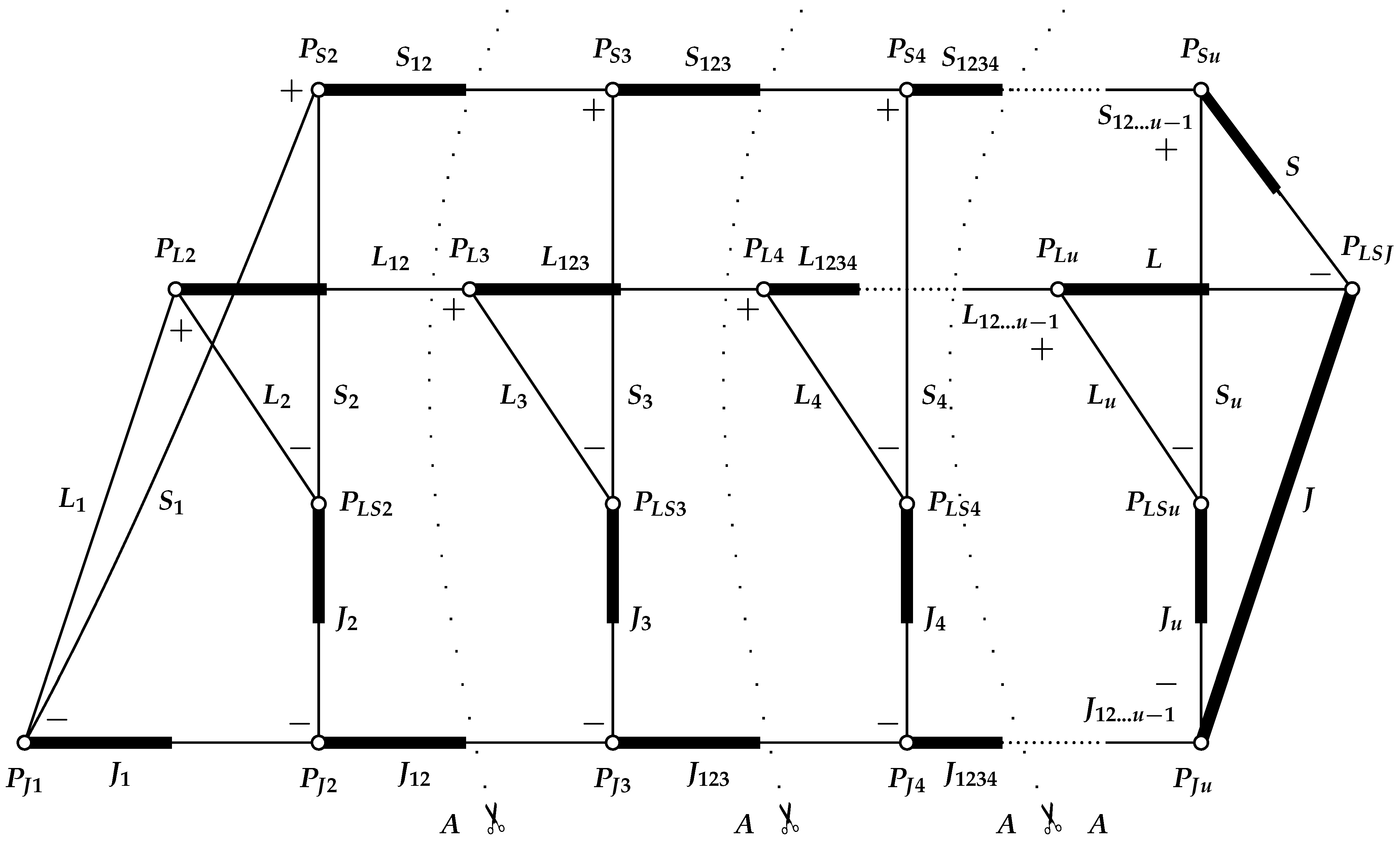
Couple the $L_i$ and $S_i$ momenta of each shell into the intermediate $J_i$ angular momentum, and then sequentially couple the intermediate $J_i$ momentum of the shells into the final J angular momentum. In this case, the $LSJ$-coupling is still valid within each shell. This coupling is called a $JJ$-coupling (see (10) and Table 1 from [8]). At this stage of the transformation, the transformation matrix in Figure 1 must be computed. We can see from Figure 1 that we couple the momenta $L_1$ and $S_1$ of the first shell into $J_1$ at the node ${\mathit{P}}_{\mathit{J}\mathbf{1}}$, we couple $L_2$ and $S_2$ of the second shell into $J_2$ at the node ${\mathit{P}}_{\mathit{L}\mathit{S}\mathbf{2}}$, and so on, until the last shell u, when angular momenta $L_u$ and $S_u$ are coupled into $J_u$ at the node ${\mathit{P}}_{\mathit{LSu}}$. After this, all the intermediate angular momenta of the shells in j space are consistently coupled into the final momentum J of the CSF at the nodes ${\mathit{P}}_{\mathit{J}\mathbf{2}}$, ${\mathit{P}}_{\mathit{J}\mathbf{3}}$, …, and ${\mathit{P}}_{\mathit{Ju}}$.

2.

Perform the transformation within the shell from the $LSJ$-coupling to the $jj$-coupling. As a result, the shell with angular momentum $J_i$ is split into two subshells with angular momenta ${\stackrel{-}{J}}_i$ and ${\stackrel{+}{J}}_i$, respectively. We have already described this transformation in Section 3 and will not return to it here because, in the general case for a CSF with any number of shells, this transformation is performed in the same way as described in Section 3.

3.

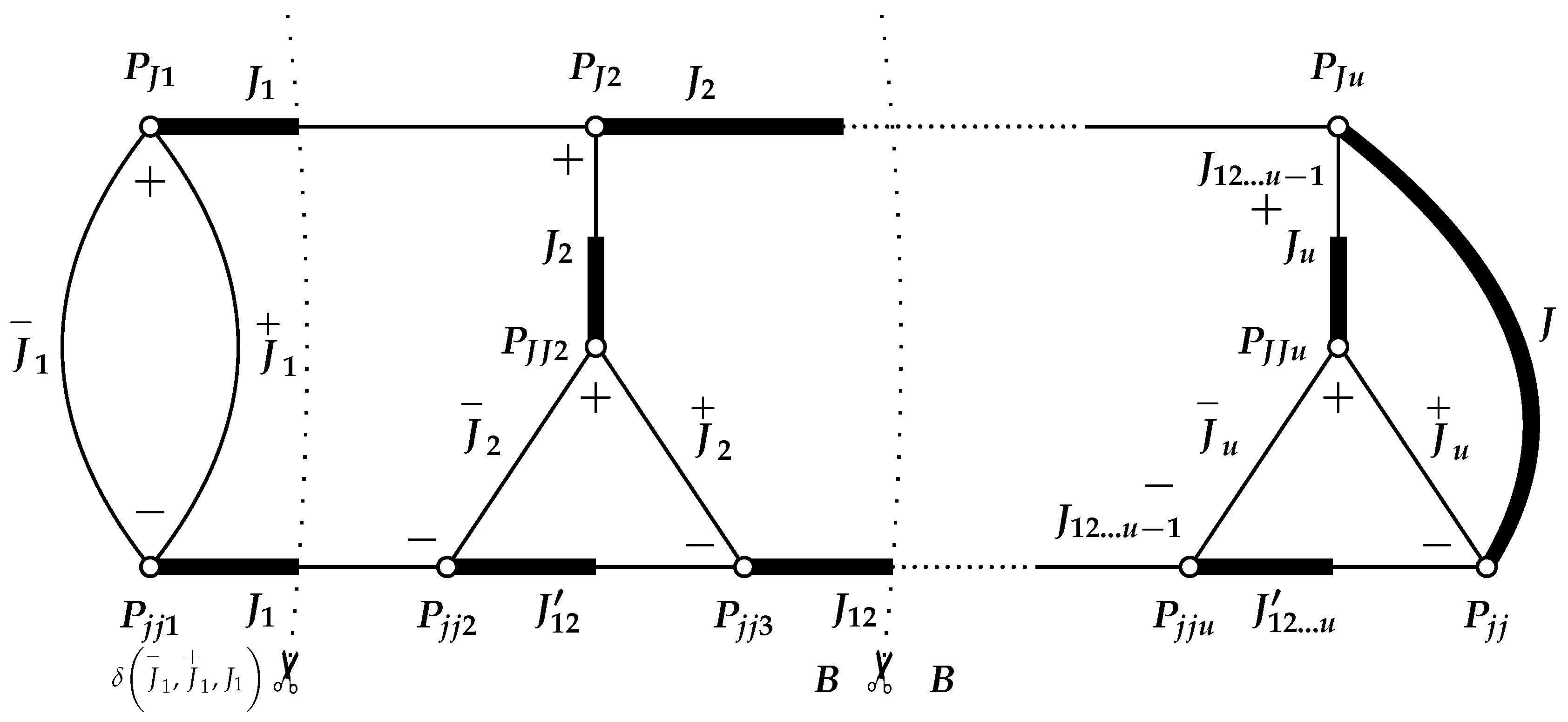
Finally, transform the angular momenta from the $JJ$-coupling scheme into the desired $jj$-coupling scheme, where the subshell angular momenta ${\stackrel{-}{J}}_i$ and ${\stackrel{+}{J}}_i$, already defined in the second stage, are coupled into the shell momentum $J_i$, which is already in the $JJ$-coupling scheme and was obtained in the first stage.

Now let us discuss stages 1 and 3 in more detail:

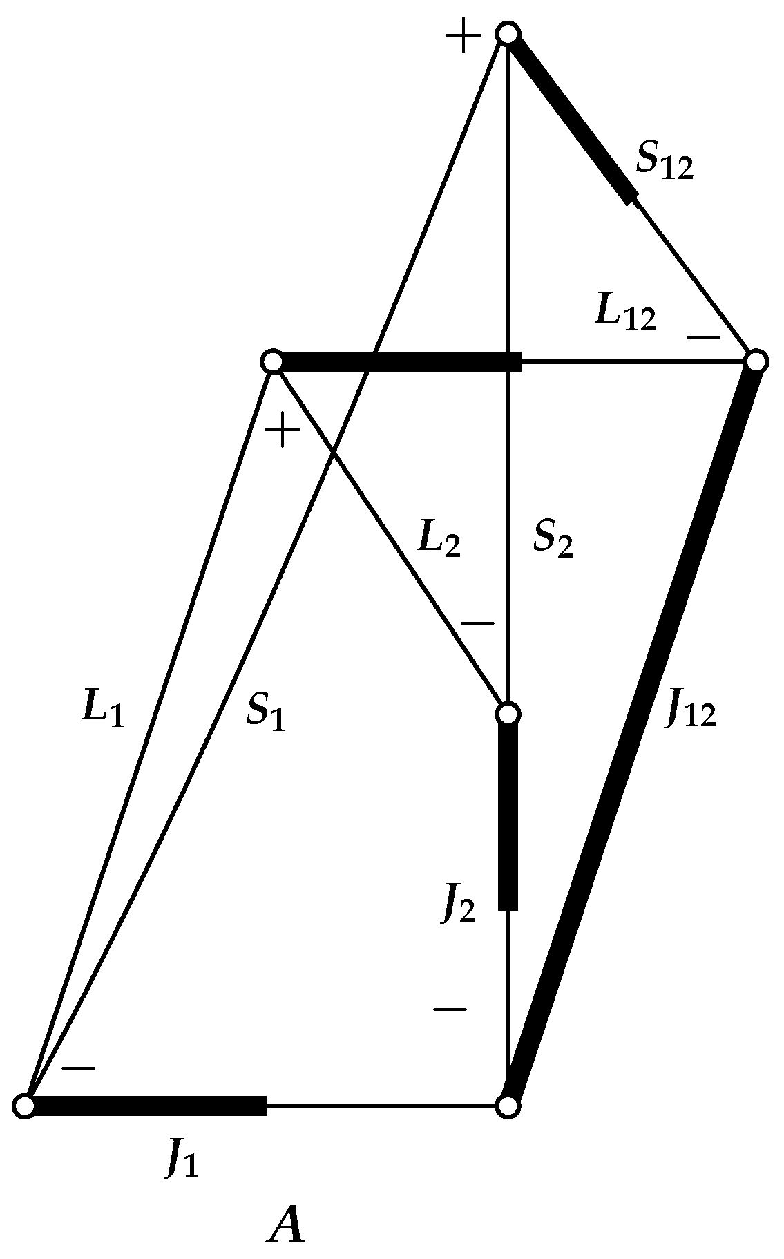
• In the first stage, as we mentioned earlier, we need to compute the transformation matrix shown in Figure 1. It is expressed as the product of Clebsch–Gordan coefficients and shell wave functions, with summation over magnetic quantum numbers. The summation can be performed by directly summing the product. However, it is much more efficient to find an algebraic expression for the transformation matrix that does not depend on the quantum numbers. This expression makes it easier and faster to find the values of the transposition matrix, especially when the CSF has several open shells, especially when it has an $n{f}^w$ open shell.
  Using the momentum theory [18], it is possible to derive this algebraic expression for the transposition matrix shown in Figure 1. This is done using the rules of graphic techniques presented in [18]. With their help, this diagram can be simplified by cutting it over three angular momentum lines: ${\mathit{J}}_{\mathbf{12}}$, ${\mathit{L}}_{\mathbf{12}}$, and ${\mathit{S}}_{\mathbf{12}}$; ${\mathit{J}}_{\mathbf{123}}$, ${\mathit{L}}_{\mathbf{123}}$, and ${\mathit{S}}_{\mathbf{123}}$; ${\mathit{J}}_{\mathbf{1234}}$, ${\mathit{L}}_{\mathbf{1234}}$, and ${\mathit{S}}_{\mathbf{1234}}$; …; ${\mathit{J}}_{\mathbf{12}\dots \mathit{u}-\mathbf{1}}$, ${\mathit{L}}_{\mathbf{12}\dots \mathit{u}-\mathbf{1}}$, and ${\mathit{S}}_{\mathbf{12}\dots \mathit{u}-\mathbf{1}}$. As we can see, there are the same $u-2$ cuts, where u is the number of open layers in CSF. For example, if the CSF consists of three open shells, there will be one such cut, and the diagram shown in Figure 1 can be expressed by two A diagrams shown in Figure 2.
  It should be noted that in the most general case, when there are u open shells, the transformation diagram splits into a product of A diagrams, consisting of $u-1$ A diagrams, all of which are topologically equivalent, with only the line notations differing. Thus, given the algebraic expression of diagram A from Figure 2, it is possible to determine the algebraic expression of the transformation matrix shown in Figure 1. Using the graphical Jucys–Bandzaitis’ method, it is easy to obtain this expression for diagram A, which is

  $$\begin{array}{c}\hfill A=\sqrt{\left[L_{12},S_{12},J_1,J_2\right]}\left\{\begin{array}{ccc}{L}_1& S_1& J_1\\ L_2& S_2& J_2\\ L_{12}& S_{12}& J_{12}\end{array}\right\}.\end{array}$$

  (15)
  Similarly, using other angular momentum graphical methods [16,17,20,21,22], we can obtain the same (Equation (15)) algebraic expression for the transformation matrix shown in Figure 2. For example, by redrawing diagram A accordingly, we can obtain a diagram that is topologically equivalent to diagram (5.3.2) in [20] and proportional to the 9j-coefficient. This is exactly what was done using the Jucys–Bandzaitis’ method [18] to obtain expression (Equation (15)).
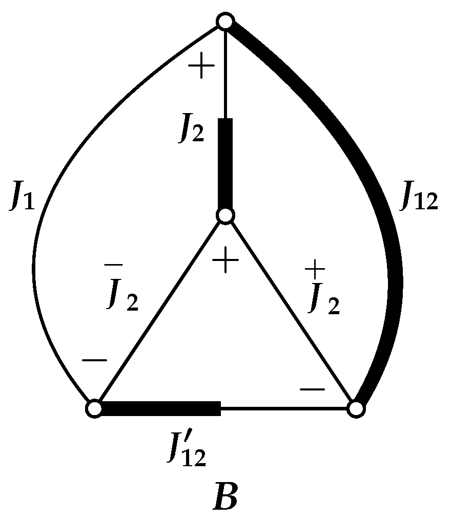
• In this third step, we need to learn how to compute the transposition matrix shown in Figure 3.
  The nodes ${\mathit{P}}_{\mathit{J}\mathbf{1}}$, ${\mathit{P}}_{\mathit{J}\mathbf{2}}$, …, ${\mathit{P}}_{\mathit{ju}}$ in this diagram correspond to the nodes ${\mathit{P}}_{\mathit{J}\mathbf{1}}$, ${\mathit{P}}_{\mathit{J}\mathbf{2}}$, …, ${\mathit{P}}_{\mathit{Ju}}$ in Figure 1. In these diagrams, they correspond to the same shell coupling, which is as it should be. In these diagrams, they correspond to the same shell coupling, as they should. Meanwhile, nodes ${\mathit{P}}_{\mathit{j}\mathit{j}\mathbf{1}}$, ${\mathit{P}}_{\mathit{j}\mathit{j}\mathbf{2}}$, …, ${\mathit{P}}_{\mathit{jju}}$ represent the angular momentum couplings we need, i.e., $jj$-coupling, when shells are divided into subshells. Nodes ${\mathit{P}}_{\mathit{j}\mathit{j}\mathbf{1}}$, …, ${\mathit{P}}_{\mathit{JJu}}$ describe the coupling of subshells into common angular momentum values $J_1$, …, $J_u$, respectively, or, in our case, when analyzing the transformation from $LSJ$-coupling to $jj$-coupling, these nodes distribute the shells’ angular momentum $J_i$ into the angular momenta ${\stackrel{-}{J}}_i$ and ${\stackrel{+}{J}}_i$ of the two corresponding subshells. This transformation diagram can also be simplified using the Jucys–Bandzaitis’ graphical technique [18]. According to it, first we cut the diagram via two lines $J_1$ (at node ${\mathit{P}}_{\mathit{J}\mathbf{1}}$) and $J_1$ (at node ${\mathit{P}}_{\mathit{j}\mathit{j}\mathbf{1}}$). Such line cutting leads to a non-zero value in the transformation matrix only when the values of these two lines coincide. Therefore, for simplicity, they have the same designation in the diagram from Figure 3. Similarly, in the remaining parts of the diagram where it is possible to cut the diagram via two lines, we will use the same principle that the lines will have the same marking. The latter cutting of the lines in the diagram at points ${\mathit{P}}_{\mathit{J}\mathbf{1}}$ and ${\mathit{P}}_{\mathit{j}\mathit{j}\mathbf{1}}$ forms a triangular delta $\delta \left({\stackrel{-}{J}}_1,{\stackrel{+}{J}}_1,J_1\right)$, similar to other graphical methods for angular momentum [16,17,20,21,22] (see, e.g., (4.3.3) from [20]). Continuing to examine the remaining diagram from left to right, we see that the next possible cut in the diagram via two lines is a cut via the $J_2$ (at node ${\mathit{P}}_{\mathit{J}\mathbf{2}}$) and $J_2$ (at node ${\mathit{P}}_{\mathit{j}\mathit{j}\mathbf{2}}$) lines. This part of the diagram, cut according to the graphical technique [18], is represented by diagram B, which is shown in Figure 4.
  There may be additional such diagram cuts, depending on the number of open layers in the CSF. Therefore, we cut the diagram using the same principle until we reach the points ${\mathit{P}}_{\mathit{Ju}}$, ${\mathit{P}}_{\mathit{JJu}}$, and ${\mathit{P}}_{\mathit{jju}}$ in the diagram. Each such cut, with the remaining part of the diagram after the last cut, when the cut is made via the lines $J_{12\dots u-1}$ (at node ${\mathit{P}}_{\mathit{Ju}}$) and $J_{12\dots u-1}$ (at node ${\mathit{P}}_{\mathit{jju}}$), leads to diagram B in Figure 4. Thus, we see that the transformation diagram in Figure 4 decomposes into a product of $u-1$ B diagrams. Using Jucys–Bandzaitis’ graphical technique [18], we find that diagram B has the following algebraic expression:

  $$\begin{array}{c}\hfill B={\left(-1\right)}^{J_1+{\stackrel{-}{J}}_2+{\stackrel{+}{J}}_2+J_{12}}\sqrt{\left[J_2,J_{12}^{\prime }\right]}\left\{\begin{array}{ccc}{\stackrel{-}{J}}_2& {\stackrel{+}{J}}_2& J_2\\ J_{12}& J_1& J_{12}^{\prime }\end{array}\right\}.\end{array}$$

  (16)
  Similarly, using other angular momentum graphical methods [16,17,20,21,22], we can obtain the same (Equation (16)) algebraic expression for the transformation matrix shown in Figure 4. For example, diagram (5.2.3) shown in [20] is topologically equivalent to diagram B shown in Figure 4. Both diagrams correspond to the 6j-coefficient. However, because Jucys–Bandziatis’ technique graphically [18] represents Clebsch–Gordan coefficients, whereas El Bas–Castel [20] represents Wigner 3-j coefficients, there are differences in phase and multipliers between these graphical representations.

Thus, taking into account the considerations presented in Section 3 regarding the transformation from $LSJ$-coupling to $jj$-coupling or from $jj$-coupling to $LSJ$-coupling in the case of a single open shell in the CSF, and what we have discussed above in this section, for any number of open shells in the CSF, we obtain the following algebraic expression for the final transformation from $LSJ$-coupling to $jj$-coupling or from $jj$-coupling to $LSJ$-coupling in the most general case, which allows us to change the coupling scheme for the CSF with an arbitrary number of shells:

$$\begin{array}{c}\hfill 〈(((((({\stackrel{-}{l}}_1^{{\stackrel{-}{w}}_1}{\stackrel{-}{\nu }}_1{\stackrel{-}{J}}_1,{\stackrel{+}{l}}_1^{(w_1-{\stackrel{-}{w}}_1)}{\stackrel{+}{\nu }}_1{\stackrel{+}{J}}_1)J_1,{\stackrel{-}{l}}_2^{{\stackrel{-}{w}}_2}{\stackrel{-}{\nu }}_2{\stackrel{-}{J}}_2)J_{12}^{\prime },{\stackrel{+}{l}}_2^{(w_2-{\stackrel{-}{w}}_2)}{\stackrel{+}{\nu }}_2{\stackrel{+}{J}}_2)J_{12}{\stackrel{-}{l}}_3^{{\stackrel{-}{w}}_3}{\stackrel{-}{\nu }}_3{\stackrel{-}{J}}_3)J_{123}^{\prime },{\stackrel{+}{l}}_3^{(w_3-{\stackrel{-}{w}}_3)}{\stackrel{+}{\nu }}_3{\stackrel{+}{J}}_3)J_{123}\dots )J\\ \hfill |((((l_1^{w_1}{\alpha }_1{L}_1{S}_1,l_2^{w_2}{\alpha }_2{L}_2{S}_2)L_{12}{S}_{12},l_3^{w_3}{\alpha }_3{L}_3{S}_3)L_{123}{S}_{123})\dots )LSJ〉\\ \hfill {\displaystyle =\left[\sum _{J_1}〈({\stackrel{-}{l}}_1^{{\stackrel{-}{w}}_1}{\stackrel{-}{\nu }}_1{\stackrel{-}{J}}_1,{\stackrel{+}{l}}_1^{(w-{\stackrel{-}{w}}_1)}{\stackrel{+}{\nu }}_1{\stackrel{+}{J}}_1)J_1{l}_1^{w_1}{\alpha }_1{L}_1{S}_1{J}_1〉\right]\prod _{i=2}^q{\left(-1\right)}^{{\stackrel{-}{J}}_i+{\stackrel{+}{J}}_i+J_{1\dots i-1}+J_{1\dots i}}\sqrt{\left[J_{12\dots i}^{\prime },J_{1\dots i-1},L_{1\dots i},S_{1\dots i}\right]}}\\ \hfill \times \sum _{J_i}\left[J_i\right]\left\{\begin{array}{ccc}{\stackrel{-}{J}}_i& {\stackrel{+}{J}}_i& J_i\\ J_{1\dots i}& J_{1\dots i-1}& J_{1\dots i}^{\prime }\end{array}\right\}\left\{\begin{array}{ccc}{L}_{1\dots i-1}& S_{1\dots i-1}& J_{1\dots i-1}\\ L_i& S_i& J_i\\ L_{1\dots i}& S_{1\dots i}& J_{1\dots i}\end{array}\right\}〈({\stackrel{-}{l}}_i^{{\stackrel{-}{w}}_i}{\stackrel{-}{\nu }}_i{\stackrel{-}{J}}_i,{\stackrel{+}{l}}_i^{(w-{\stackrel{-}{w}}_i)}{\stackrel{+}{\nu }}_i{\stackrel{+}{J}}_i)J_i{l}_i^{w_i}{\alpha }_i{L}_i{S}_i{J}_i〉.\end{array}$$

(17)

Here we see a u-pair product, where each pair consists of 6j-coefficients, 9j-coefficients and a $jj$–$LS$ transformation matrix for the shell of equal electrons (Equation (12)) that changes the interaction within the shell. The 9j-coefficient comes from the transformation matrix shown in Figure 1 and is graphically represented by diagram A (see Figure 2). The 6j-coefficient comes from the transformation matrix shown in Figure 3 and is graphically represented by diagram B (see Figure 4). The last coefficient is related to the $jj$–$LS$ transformation matrix for the shell of equal electrons, which changes the coupling within the shell, and is described in Section 3. As we can see, another such $jj$–$LS$ transformation matrix for the shell of equal electrons (Equation (12)) appears before the multiplication sign for the first shell because the 6j- and 9j-coefficients appear only when the number of open shells is two or more.

In the case of a single open shell, the expression (Equation (17)) becomes the transformation matrix given in Equations (10) and (11). As we can see, Equation (17) is suitable for both the CSF transformation from $jj$-coupling to $LSJ$-coupling and from $LSJ$-coupling to $jj$-coupling.

In the case of two open shells, the expression is also simple. In this case, Equation (17) is reduced to an expression in which we have one 6j-coefficient and one 9j-coefficient and two $jj$–$LS$ transformation matrices for the shell of equal electrons. This expression is the same as (21) from [12].

5. Implementation of the Methodology in Programs

There are several programs [7,8,23,24] based on the methodology presented in the paper. The Racah VI program [23] is written in the Maple programming language and is designed to perform various manipulations of algebraic formulas within the framework of atomic theory and to perform simple calculations for atoms or ions with one or two open shells in the CSF in terms of $LSJ$-coupling. In this case, the program uses simple formulas (Equation (11), as well as (21) from [12]). This program can also serve as an electronic table of $jj$–$LS$ transformation matrix for the shell of equal electrons, allowing us to quickly and easily obtain the desired values for these coefficients. This is particularly important when searching for a transformation matrix for $n{f}^w$ shell because there are a very large number of these coefficients. For example, in the case of $n{f}^6$, we have 9393 such coefficients, of which 7313 are non-zero.

The Coupling program [8] is written in the Fortran programming language. It is designed to determine the optimal ASF coupling when ASF is obtained using the CI, MCHD, RCI, and MCDF methods. The program is limited to one- and two-shell systems in terms of $LSJ$-coupling, and thus, it is written based on Equation (11) and (21) from [12].

Programs [7,24] are written in the Fortran programming language and are intended for large-scale calculations. Therefore, they use Equation (17). These two programs are compatible with the Atsp [4] and Grasp [5,6] software packages and libraries libang77 [25] and librang90 [26], i.e., they use $jj$–$LS$ transformation matrix for the shell of equal electrons that are compatible with the CFP coefficients [12,15] available in these programs and libraries. We would also like to note that program jj2lsj [7] is one of the few existing programs that integrates the Atsp and Grasp computer packages. With the help of the jj2lsj program, it is possible to convert the ASF expansion coefficients obtained from calculations in relativistic atomic theory with Grasp (from Grasp output files <name>.m or <name>.cm and <name>.c) to expansion coefficients corresponding to non-relativistic atomic theory (to Atsp output files <name>.c and <name>.j), and to convert the ASF from $LSJ$-coupling (from Atsp output files <name>.c and <name>.j) to $jj$-coupling (to file <name>.jj.lbl) with the program coupling [8].

As we can see from the theory described above, these programs [7,24] perform calculations in the following order:

1.

The necessary and complete CSF list in the $LSJ$-coupling scheme based on the existing CSF list in the $jj$-coupling is generated, and this corresponds to the operation of such programs as gencl [27] or lsgen [28].

2.

Transformation matrices are computed using a general expression (Equation (17)), with calculations that are partly reminiscent of spin-angular integration in the Atsp (either in nonh [29] or breit [30] or mltpol [31]) and Grasp (either in genmcp [32] or mcp [33] or rangular [5,6]) packages.

3.

The expansion coefficients $a_{ij}$ from Equation (3) for ASF are found in the $LSJ$-coupling according to Equation (6), which partially corresponds to the calculation of atomic characteristics, such as transition characteristics, using the lstr and lsjtr programs [34].

• Therefore, at first glance, this transformation seems to be a simple task. However, as we can see, the ASF transformation from $jj$-coupling to $LSJ$-coupling splits into three types of tasks, similar to those performed by three different program types in the Atsp or Grasp packages. With this in mind, and considering that a large number of $LS$–$jj$ transformation matrices for the shell of equal electrons are used to transform the $n{f}^w$ shell, the operation of programs [7,24] may sometimes require more computing time.

The most suitable program for transformation of the ASF from $jj$-coupling to $LSJ$-coupling in atomic theory is jj2lsj [7]. The program jj2lsj is maximally optimized in terms of the algorithm. The computational complexity of the jj2lsj algorithm does not depend on the number of open shells because it is based on an algebraic expression whose form is not affected by the number of open shells. The methodology presented in the paper is both attractive and easy to implement in code. The program’s calculation speed depends on the specifics of the task being computed. The program computation time mostly depends on the number of open shells in the CSF and the type of shells in the CSF, i.e., the speed is particularly slowed when an open f shell has occupation numbers 6, 7, or 8. In this case, such a transformation can take longer than when the CSF consists of more open shells but does not include an open f shell. In addition, to speed up calculations performed only for level identification in $LSJ$-coupling, when the program’s default option is used, only a partial ASF transformation is performed, transforming only CSFs with the highest expansion coefficients. The complete ASF transformation is performed only upon the user’s specific request. Naturally, in this case, the program’s operation is extended.

jj2lsj [7] is an open source program. Since it is integrated into the Grasp2018 computer package, it is available on GitHub in the Grasp2018 repositories. The author is not aware of an existing analogous jj2lsj [7] programs that would perform an ASF transformation in the most general case where the CSF consists of any number of open shells.

6. Conclusions

The developed methodology allows us to transform the atomic state function, which consists of any number of configuration state functions, each with any number of open shells, from $jj$-coupling to $LSJ$-coupling, and vice versa. This methodology has been implemented in several programs, including jj2lsj, which is suitable for large-scale calculations. jj2lsj can be used with any software package based on $jj$-coupling that uses CFPs matched to the $LS$-$jj$ transformation matrices for the shell of equal electrons, as proposed in this paper.

References

- Fischer, C.F.; Godefroid, M.; Brage, T.; Jönsson, P.; Gaigalas, G. Advanced multiconfiguration methods for complex atoms: I. Energies and wave functions. J. Phys. B At. Mol. Phys. 2016, 49, 182004. [Google Scholar] [CrossRef]
- Grant, I.P. Relativistic Quantum Theory of Atoms and Molecules: Theory and Computation; Atomic, Optical and Plasma Physics; Springer: New York, NY, USA, 2007. [Google Scholar] [CrossRef]
- Rudzikas, Z. Theoretical Atomic Spectroscopy; Cambridge Monographs on Atomic, Molecular and Chemical Physics; Cambridge University Press: Cambridge, MA, USA, 1997. [Google Scholar] [CrossRef]
- Froese Fischer, C.; Tachiev, G.; Gaigalas, G.; Godefroid, M. An MCHF atomic-structure package for large-scale calculations. Comput. Phys. Commun. 2007, 176, 559–579. [Google Scholar] [CrossRef]
- Jönsson, P.; Gaigalas, G.; Bieroń, J.; Froese Fischer, C.; Grant, I. New version: Grasp2K relativistic atomic structure package. Comput. Phys. Commun. 2013, 184, 2197. [Google Scholar] [CrossRef]
- Fischer, C.F.; Gaigalas, G.; Jönsson, P.; Bieroń, J. GRASP2018—A Fortran 95 version of the General Relativistic Atomic Structure Package. Comput. Phys. Commun. 2019, 237, 184–187. [Google Scholar] [CrossRef]
- Gaigalas, G.; Froese Fischer, C.; Rynkun, P.; Jönsson, P. JJ2LSJ Transformation and Unique Labeling for Energy Levels. Atoms 2017, 5, 6. [Google Scholar] [CrossRef]
- Gaigalas, G. COUPLING: The program for searching optimal coupling scheme in atomic theory. Comput. Phys. Commun. 2021, 261, 107772. [Google Scholar] [CrossRef]
- Froese Fischer, C. The Hartree-Fock Method for Atoms: A Numerical Approach; John Wiley and Sons: New York, NY, USA, 1977. [Google Scholar]
- Froese Fischer, C.; Brage, T.; Jönsson, P. Computational Atomic Structure: An MCHF Approach; Institute of Physics Publishing: Bristol, PA, USA, 1997. [Google Scholar] [CrossRef]
- Cowan, R.D. The Theory of Atomic Structure and Spectra; Los Alamos Series in Basic and Applied Sciences; University of California Press: Berkeley, CA, USA, 1981. [Google Scholar]
- Gaigalas, G.; Žalandauskas, T.; Rudzikas, Z. LS—jj transformation matrices for a shell of equivalent electrons. At. Data Nucl. Data Tables 2003, 84, 99–190. [Google Scholar] [CrossRef]
- Calvert, J.B.; Tuttle, E.R. The jj-LS Transformation Matrices for Three or More Equivalent p or d Electrons. Il Nuovo C. B 1979, 54, 413–425. [Google Scholar] [CrossRef]
- Childs, W.J. Matrix Elements of Hyperfine Structure Operators in the SL and jj Representations for the s, pN, and dN Configurations and the SL–jj Transformation. At. Data Nucl. Data Tables 1997, 67, 1–70. [Google Scholar] [CrossRef]
- Gaigalas, G.; Žalandauskas, T.; Rudzikas, Z. Analytical Expressions for Special Cases of LS-jj Transformation matrices for a Shell of Equivalent Electrons. Lith. J. Phys. 2001, 41, 226. [Google Scholar]
- Jucys, A.; Levinson, I.; Vanagas, V. Mathematical Apparatus of the Angular Momentum Theory; Israel Program for Scientific Translations: Jerusalem, Israel, 1963. [Google Scholar]
- Brink, D.; Satchler, G. Angular Momentum; Clarendon Press: Oxford, UK, 1968. [Google Scholar]
- Jucys, A.; Bandzaitis, A. Theory of Angular Momentum in Quantum Mechanics; Mokslas: Vilnius, Lithuania, 1977. [Google Scholar]
- Jucys, A.; Savukynas, A. Mathematical Foundations of the Atomic Theory; Mokslas: Vilnius, Lithuania, 1973. [Google Scholar]
- El_Baz, E.; Castel, B. Graphical Methods of Spin Algebras in Atomic, Nuclear and Particle Physics; Marcel Dekker, Inc.: New, York, NY, USA, 1972. [Google Scholar]
- Varshalovich, D.; Moskalev, A.; Khersonskii, V. Quantum Theory of Angular Momentum; World Scientific: Singapore, 1988. [Google Scholar] [CrossRef]
- Balcar, E.; Lovesey, S.W. Introduction to the Graphical Theory of Angular Momentum: Case Studies; Springer: Berlin/Heidelberg, Germany, 2009. [Google Scholar] [CrossRef]
- Gaigalas, G.; Fritzsche, S. Maple procedures for the coupling of angular momenta. VI. LS-jj transformations. Comput. Phys. Commun. 2002, 149, 39–60. [Google Scholar] [CrossRef]
- Gaigalas, G.; Žalandauskas, T.; Fritzsche, S. Spectroscopic {LSJ} notation for atomic levels obtained from relativistic calculations. Comput. Phys. Commun. 2004, 157, 239–253. [Google Scholar] [CrossRef]
- Gaigalas, G. A Program Library for Computing Pure Spin-Angular Coefficients for One- and Two-Particle Operators in Non-Relativistic Atomic Theory. Atoms 2026. in preparation. [Google Scholar]
- Gaigalas, G. A program library for computing pure spin-angular coefficients for one- and two-particle operators in relativistic atomic theory. Atoms 2022, 10, 129. [Google Scholar] [CrossRef]
- Fischer, C.F.; Liu, B. A program to generate configuration-state lists. Comput. Phys. Commun. 1991, 64, 406–416. [Google Scholar] [CrossRef]
- Sturesson, L.; Froese Fischer, C. LSGEN: A program to generate configuration state lists of LS coupled basis functions. Comput. Phys. Commun. 1993, 74, 432. [Google Scholar] [CrossRef]
- Hibbert, A.; Froese Fischer, C. A general program for computing angular integrals of the non-relativistic Hamiltonian with non-orthogonal orbitals. Comput. Phys. Commun. 1991, 64, 417–430. [Google Scholar] [CrossRef]
- Hibbert, A.; Glass, R.; Froese Fischer, C. A general program for computing angular integrals of the Breit-Pauli Hamiltonian. Comput. Phys. Commun. 1991, 64, 455–472. [Google Scholar] [CrossRef]
- Fischer, C.F.; Godefroid, M.R.; Hibbert, A. A program for performing angular integrations for transition operators. Comput. Phys. Commun. 1991, 64, 486–500. [Google Scholar] [CrossRef]
- Parpia, F.; Froese Fischer, C.; Grant, I. GRASP92: A package for large-scale relativistic atomic structure calculations. Comput. Phys. Commun. 1996, 94, 249–271. [Google Scholar] [CrossRef]
- Jönsson, P.; He, X.; Froese Fischer, C.; Grant, I. The grasp2K relativistic atomic structure package. Comput. Phys. Commun. 2007, 177, 597–622. [Google Scholar] [CrossRef]
- Fischer, C.F.; Godefroid, M.R. Programs for computing {LS} and {LSJ} transitions from {MCHF} wave functions. Comput. Phys. Commun. 1991, 64, 501–519. [Google Scholar] [CrossRef]
Disclaimer/Publisher’s Note: The statements, opinions and data contained in all publications are solely those of the individual author(s) and contributor(s) and not of MDPI and/or the editor(s). MDPI and/or the editor(s) disclaim responsibility for any injury to people or property resulting from any ideas, methods, instructions or products referred to in the content. |
© 2026 by the author. Licensee MDPI, Basel, Switzerland. This article is an open access article distributed under the terms and conditions of the Creative Commons Attribution (CC BY) license.
Share and Cite
Gaigalas, G. jj to LSJ Transformation for Configuration State Functions with an Arbitrary Number of Open Shells. Atoms 2026, 14, 20. https://doi.org/10.3390/atoms14030020
Gaigalas G. jj to LSJ Transformation for Configuration State Functions with an Arbitrary Number of Open Shells. Atoms. 2026; 14(3):20. https://doi.org/10.3390/atoms14030020
Chicago/Turabian StyleGaigalas, Gediminas. 2026. "jj to LSJ Transformation for Configuration State Functions with an Arbitrary Number of Open Shells" Atoms 14, no. 3: 20. https://doi.org/10.3390/atoms14030020
APA StyleGaigalas, G. (2026). jj to LSJ Transformation for Configuration State Functions with an Arbitrary Number of Open Shells. Atoms, 14(3), 20. https://doi.org/10.3390/atoms14030020