Multiplatform Computing of Transition Probabilities in Os V

Abstract

Osmium is an element of the Periodic Table with an atomic number Z equal to 76. In Tokamaks with divertors made of tungsten ($Z=74$), it is produced in the neutron-induced transmutation of the latter. Therefore one can expect that their sputtering may generate ionic impurities of all possible charge states in the fusion plasma. As a consequence, these could contribute to radiation losses in these controlled nuclear devices. The knowledge of radiative rates in all the spectra of osmium is thus important in this field. In this framework, a multiplatform approach has been used to determine the Os V radiative properties and estimate their accuracy. The transition probabilities have been computed for the 2677 electric dipole (E1) transitions falling in the spectral range from 400 Å to 12,000 Å. Three independent atomic structure models have been considered; one based on the fully relativistic ab initio multiconfiguration Dirac–Hartree–Fock (MCDHF) method and two based on the semi-empirical pseudo-relativistic Hartree–Fock (HFR) method.

1. Introduction

Tungsten (W) will be used as a plasma-facing material in future fusion devices such as ITER [1] and will be bombarded by an intense neutron flux generated by deuterium–tritium fusion reactions. Osmium (Os) will then be produced by transmutation of tungsten by neutron capture [2]. The former element, as an impurity in all stages of ionization, could propagate into the fusion plasma. Thus, all these ions could radiate and this could contribute to radiation losses in the reactor’s energy balance. Their radiative properties are therefore of interest in nuclear fusion.

Concerning the fifth spectrum of osmium (Os V), there is only one publication that is available in the literature. Azarov et al. [3] photographed the osmium spectrum from 225 Å to 2100 Å using the 3 m normal-incidence spectrograph, equipped with a 2400 L/mm grating, of the Physics Department of St. Francis Xavier University. The source was a low-inductance triggered spark. In that work, they classified 703 Os V lines belonging to $(5{\mathrm{d}}^5+5{\mathrm{d}}^{3}6\mathrm{s})-5{\mathrm{d}}^{3}6\mathrm{p}$. In total, 57 levels of the even-parity configurations $(5{\mathrm{d}}^5+5{\mathrm{d}}^{3}6\mathrm{s})$ and 89 levels of the odd-parity configuration $5{\mathrm{d}}^{3}6\mathrm{p}$ were determined in this analysis with the help of a semi-empirical atomic structure model based on orthogonal operator technique. They also published the computed transition probabilities of their 703 classified E1 transitions, but their accuracies were not evaluated. Moreover, extending the data to a larger number of emission lines should be valuable in radiation loss modeling, but the latter is beyond the scope of the present paper.

In this analysis, we present a multiplatform approach to compute the transition probabilities in the spectrum of four times ionized osmium in which their accuracies have been estimated by using three independent atomic structure models. In Section 2, the computational methods and the models are described. The results are given and discussed in Section 3. The conclusions are presented in Section 4.

2. Atomic Structure Computations

Three independent computations have been performed in order to determine the Os V radiative parameters. The semi-empirical HFR method [4] has been employed for two of them, relying on available experimental level energies. Instead, in the third calculation, a purely ab initio relativistic method, namely MCDHF [5], has been considered. The details of the three computations are given in the following subsections.

2.1. The HFR Calculations

The Hartree–Fock method including relativistic corrections (HFR), developed by R. D. Cowan [4], was employed. In this framework, the atomic state functions (ASFs) are expressed as linear combinations of configuration state functions (CSFs). These CSFs are $LSJ$-coupled Slater determinants constructed from non-relativistic one-electron orbitals, ${\varphi }_{nl{m}_l{m}_s}(r,\theta ,\phi ,s_z)$, where $s_z$ denotes the projection of the electron spin along the z-axis [4].

The radial components of the one-electron orbitals were obtained by solving the monoconfigurational HFR radial equations derived from the variational minimization of the configuration-average energy $E_{av}$ for each non-relativistic configuration included in the model. The relativistic mass–velocity and Darwin corrections were incorporated at this stage. Subsequently, the expansion (mixing) coefficients were determined by diagonalizing the multiconfiguration Hamiltonian matrix, augmented by the spin–orbit interaction operator.

The model considered here follows the model HFR+CP(B) used in Tm-like W III [6], which was successful in predicting accurate lifetimes in good agreement with time-resolved laser-induced fluorescence (TR-LIF) measurements. A similar model was also applied more recently in Tm-like Re IV [7].

The ASFs were expanded over the following sets of interacting configurations: $5{\mathrm{d}}^4$ + $5{\mathrm{d}}^{3}n\mathrm{s}(n=6-8)$ + $5{\mathrm{d}}^{2}6{\mathrm{s}}^2$ + $5{\mathrm{d}}^{2}6\mathrm{s}n\mathrm{s}(n=7-8)$ + $5{\mathrm{d}}^{3}6\mathrm{d}$ + $5{\mathrm{d}}^{2}6\mathrm{s}6\mathrm{d}$ + $5\mathrm{d}6{\mathrm{s}}^{2}6\mathrm{d}$ + $5{\mathrm{d}}^{2}6{\mathrm{p}}^2$ for the even parity and $5{\mathrm{d}}^{3}n\mathrm{p}(n=6-8)$ + $5{\mathrm{d}}^{2}6\mathrm{s}n\mathrm{p}(n=6-8)$ + $5\mathrm{d}6{\mathrm{s}}^{2}6\mathrm{p}$ for the odd parity.

As a first step, all Slater integrals entering the Hamiltonian were uniformly reduced by a factor of 0.85, following the common procedure adopted for moderately charged ions to account for the influence of neglected highly excited interacting configurations on the mixing coefficients [4].

Subsequently, a semi-empirical least-squares fitting was carried out. This procedure involved adjusting selected radial Hamiltonian parameters—including configuration-average energies, Slater integrals, and spin–orbit coupling constants—so as to minimize the discrepancies between the calculated eigenvalues of the Hamiltonian and the experimental energy levels reported in the literature [3].

The mean deviations obtained from the fitting were 112 cm⁻¹ for the even parity, considering all 57 experimentally known levels belonging to the $5{\mathrm{d}}^4$ and $5{\mathrm{d}}^{3}6\mathrm{s}$ configurations, and 229 cm⁻¹ for the odd parity, including all 89 known levels of the $5{\mathrm{d}}^{3}6\mathrm{p}$ configuration. These deviations are slightly larger than those reported by Azarov et al. [3], who achieved values of 14.6 and 37.2 cm⁻¹ for the even- and odd-parity levels, respectively. However, it is important to highlight that our calculations incorporate a significantly greater number of interacting configurations. This expanded scope often results in more intricate adjustment processes due to the increased complexity of mixing within the eigenvector compositions. We report the radial parameters for the known electronic configurations, i.e., $5{\mathrm{d}}^4$, $5{\mathrm{d}}^{3}6\mathrm{s}$ and $5{\mathrm{d}}^{3}6\mathrm{p}$, adopted for the calculation of the transition probabilities in Os V in Table 1. For the other configurations, the Slater and spin–orbit parameters were kept fixed, respectively, to 85% and to 100% of their HFR values.

Table 1. Radial parameters (in cm⁻¹) adopted for the known electronic configurations in our HFR model for Os V.

Configuration	Parameter	Ab Initio	Fitted	Ratio
Even Parity
$5{\mathrm{d}}^4$	$E_{av}$	37,599	36,357	/
	$F^2\left(5d5d\right)$	68,736	57,082	0.83
	$F^4\left(5d5d\right)$	45,955	39,602	0.86
	${\zeta }_{5d}$	4315	4113	0.95
$5{\mathrm{d}}^{3}6\mathrm{s}$	$E_{av}$	108,054	103,793	/
	$F^2\left(5d5d\right)$	70,282	57,890	0.82
	$F^4\left(5d5d\right)$	47,111	40,340	0.86
	${\zeta }_{5d}$	4315	4113	0.95
	$G^2\left(5d6s\right)$	22,240	19,024	0.86
$5{\mathrm{d}}^4-5{\mathrm{d}}^{3}6\mathrm{s}$	$R^2(5d5d,5d6s)$	−26,978	−24,382	0.90
Odd Parity
$5{\mathrm{d}}^{3}6\mathrm{p}$	$E_{av}$	184,644	182,094	/
	$F^2\left(5d5d\right)$	70,702	58,172	0.82
	$F^4\left(5d5d\right)$	47,429	40,970	0.86
	${\zeta }_{5d}$	4588	4397	0.96
	${\zeta }_{6p}$	10,317	11,575	1.12
	$F^2\left(5d6p\right)$	30,873	25,419	0.82
	$G^1\left(5d6p\right)$	12,537	9807	0.78
	$G^3\left(5d6p\right)$	10,942	6855	0.63

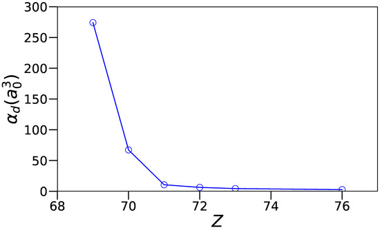
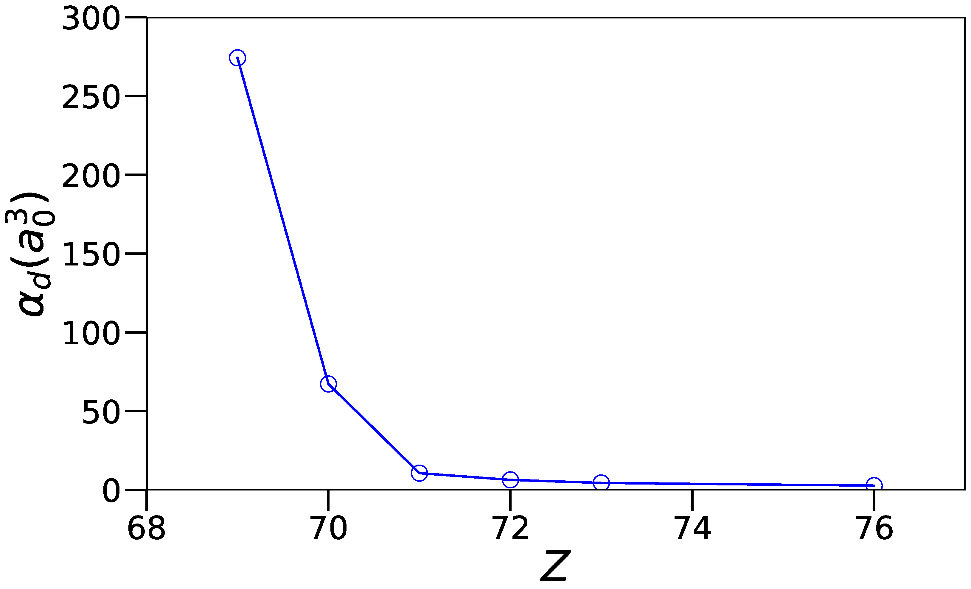
In the determination of the transition probabilities, two different calculations were carried out. In the first one, referred as HFR + CPOL, the core-polarization effects on the transition dipole operator were considered [8,9]. The cut-off radius of the ionic core was taken as the HFR value of the average radius of the outermost core orbital, namely ${⟨5d\left|r\right|5d⟩}_{HFR}=1.530a_0$. Concerning the dipole polarizability of the ionic core, ${\alpha }_d$, a value of ${\alpha }_d=2.70a_0^3$ was extrapolated from the tabulated values reported in Fraga et al. [10] along the Tm-like sequence (see Figure 1). The second calculation, referred to as HFR, neglected these effects.

Figure 1. Trend of the dipole polarizability, ${\alpha }_d$ in $a_0^3$, as a function of the atomic number Z along the thulium ($Z=69$) isoelectronic sequence. The value of ${\alpha }_d=2.70a_0^3$ for Os V ($Z=76$) has been extrapolated from those tabulated in Fraga et al. [10] for $Z=69-73$.

2.2. The MCDHF-RCI Calculations

The second method used in this work was the MCDHF method [5] coded in the GRASP2018 computer package [11] and in its extension GRASPG based on configuration state function generators (CSFGs) [12,13]. The latter are an efficient way of ordering and generating CSFs to save computation time and memory based on the fact that the spin-angular coefficient calculation does not depend on the spin-orbital’s principal quantum numbers [12].

The atomic state function (ASF), $\Psi (\alpha \Pi J{M}_J)$, characterized by the parity $\Pi$, the total angular momentum J, and its magnetic projection $M_J$, is expressed as a linear combination of configuration state functions (CSFs), $\Phi (\gamma \Pi J{M}_J)$. The labels $\alpha$ and $\gamma$ denote specific ASFs and CSFs, respectively.

In the present work, the CSFs are constructed from $jj$-coupled polyelectronic Slater determinants built from one-electron spin-orbitals, ${\varphi }_{n\kappa m}(r,\theta ,\phi )$. The associated large and small radial components are obtained as solutions of the radial integro-differential equations arising in the multiconfiguration Dirac–Hartree–Fock (MCDHF) framework. The relativistic quantum number $\kappa$ is linked to the non-relativistic orbital angular momentum quantum number ℓ and to the total angular momentum j of the electron [5].

The CSF expansions are generated from a selected set of configurations referred to as the multireference (MR), which includes the target configurations as well as others that interact strongly with them. Additional CSFs are produced by allowing single and/or multiple excitations from the occupied orbitals of the MR into an active set of orbitals (AS). In the following, the AS is denoted by a set of $n_{\max }\mathit{\ell }$, where $n_{\max }$ represents the highest principal quantum number considered for a given value of the non-relativistic orbital quantum number ℓ associated with an excited subshell.

In order to represent the known configurations of Os V [3], i.e., $5{\mathrm{d}}^4$, $5{\mathrm{d}}^{3}6\mathrm{s}$ and $5{\mathrm{d}}^{3}6\mathrm{p}$, the following strategy has been considered comparable to the one used for Re IV [7]. Two separate optimizations were carried out, one for each parity.

In the first step, in the even parity, the core 1s-5p and targeted orbitals 5d and 6s were optimized by minimizing an energy functional built from all 81 levels of the MR ($5{\mathrm{d}}^4$ + $5{\mathrm{d}}^{3}6\mathrm{s}$ + $5{\mathrm{d}}^{2}6{\mathrm{s}}^2$) with symmetries $J^{\Pi }=0^e-6^e$ during a self-consistent field (SCF) MCDHF Extended Average Level (EAL) procedure [5,11]. Regarding the odd parity, a similar MCDHF-EAL procedure was followed that optimized all the core and the targeted 5d and 6p orbitals by minimizing all 186 levels of the MR ($5{\mathrm{d}}^{3}6\mathrm{p}$ + $5{\mathrm{d}}^{2}6{\mathrm{s}}^{2}6\mathrm{p}$) with symmetries $J^{\Pi }=1^o-7^o$.

The next steps consisted of including some correlation in the ASF expansions of the MRs of both parities. First, valence correlation was included by considering all the single (S) and double (D) excitations from the MR valence orbitals to the AS $\{7\mathrm{s},6\mathrm{p},6\mathrm{d},5\mathrm{f}\}$ and the AS $\{7\mathrm{s},7\mathrm{p},6\mathrm{d},5\mathrm{f}\}$ in the even and odd parities, respectively. These generated a total of 2529 CSFs in the even parity and 6196 CSFs in the odd parity. Thereafter, CSFs that interacted with those of the MR were selected. This reduced these numbers to 2470 CSFs in the even parity and 6015 CSFs in the odd parity. The first layer of correlation orbitals, namely 7s, 6p, 6d and 5f for the even parity and 6s, 7p, 6d and 5f for the odd parity, were optimized by minimizing an energy functional built on all the levels of the respective MRs in an Extended Optimal Level (EOL) procedure [5,11], with all the other orbitals being kept fixed to the values of the preceding step.

The same procedure was followed to add another three layers of valence–valence (VV) correlation orbitals by considering the following ASs: $\{8\mathrm{s},7\mathrm{p},7\mathrm{d},6\mathrm{f}\}$, $\{9\mathrm{s},8\mathrm{p},8\mathrm{d},7\mathrm{f}\}$ and $\{10\mathrm{s},9\mathrm{p},9\mathrm{d},8\mathrm{f}\}$ for the even parity and $\{8\mathrm{s},8\mathrm{p},7\mathrm{d},6\mathrm{f}\}$, $\{9\mathrm{s},9\mathrm{p},8\mathrm{d},7\mathrm{f}\}$ and $\{10\mathrm{s},10\mathrm{p},9\mathrm{d},8\mathrm{f}\}$ for the odd parity. There, the respective numbers of CSFs before and after the reduction by interaction with the respective MRs, using a Dirac–Coulomb–Breit (DCB) Hamiltonian, were the following: in the even parity, 9244 and 9087 for two layers, 20,226 and 19,919 for three layers and 35,475 and 34,966 for four layers, and in the odd parity, 20,782 and 20,251 for two layers, 43,998 and 42,845 for three layers and 75,844 and 73,797 for four layers.

Finally, core–valence (CV) and core–core (CC) correlation effects were incorporated through a subsequent relativistic configuration interaction (RCI) calculation. In this step, the orbitals optimized in the previous stages were retained, and the Dirac–Coulomb–Breit (DCB) Hamiltonian, supplemented by quantum electrodynamics (QED) corrections, was constructed and diagonalized. For this to be achieved, S and D promotions from the 4f, 5s and 5p core orbitals of the respective even and odd MRs were added to our four-layer VV expansion. In order to keep the size of the problem under control, the following restrictions were activated: only three layers were considered and only one hole was allowed in the core orbitals for the CV correlation, whereas, for the CC correlation, only one correlation layer was allowed with no restriction to the core orbital occupations, but with the additional constraint of doubly occupied correlation orbitals. This generated 2,075,126 CSFs in the even parity and 6,154,289 CSFs in the odd parity. Those numbers were reduced to 1,280,833 and 3,635,854 in, respectively, the even and odd parities after interacting with the CSFs of the respective MRs.

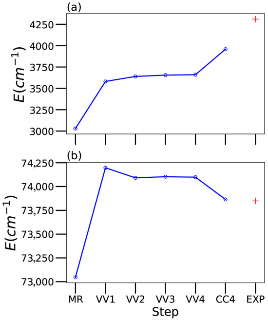
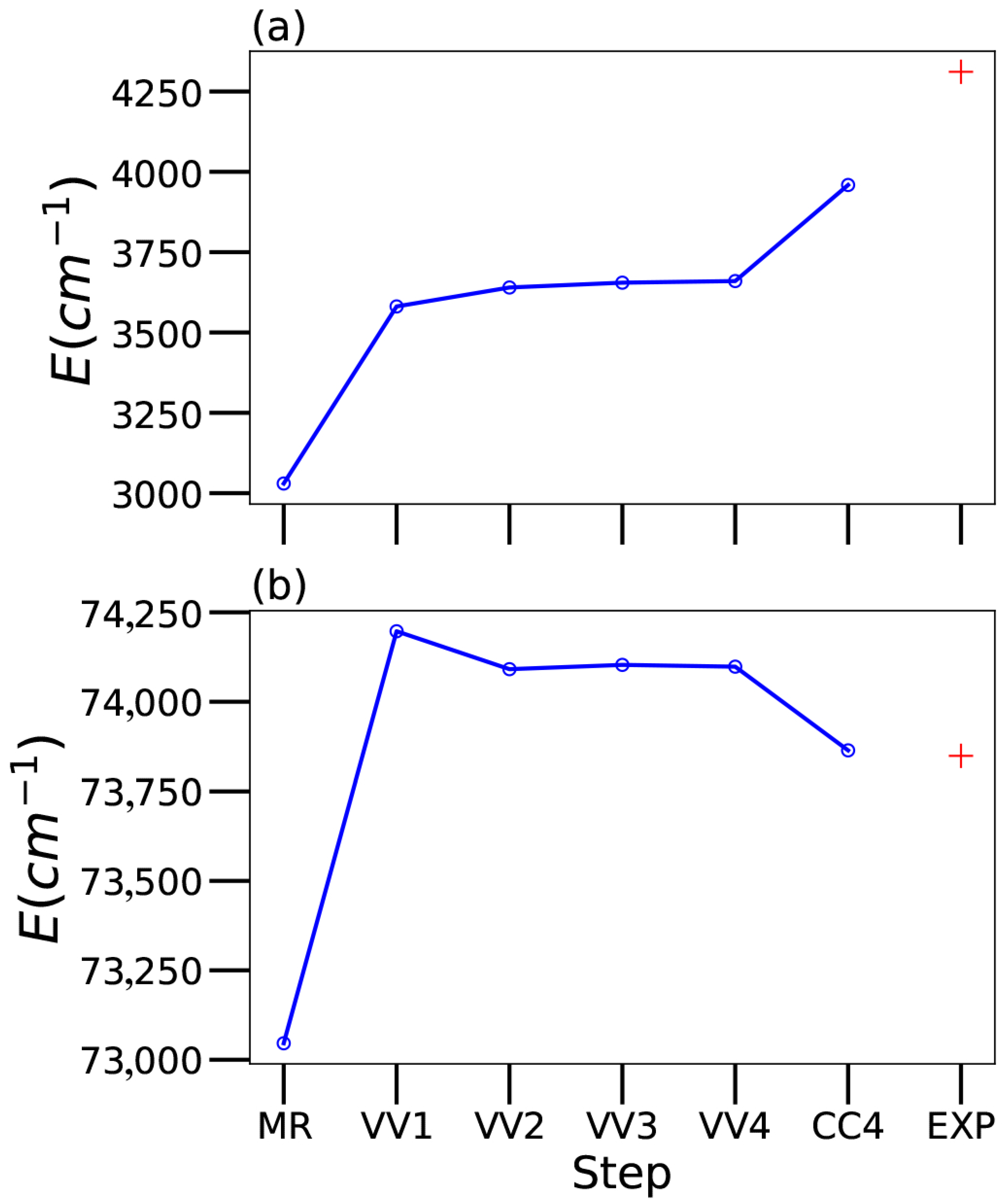
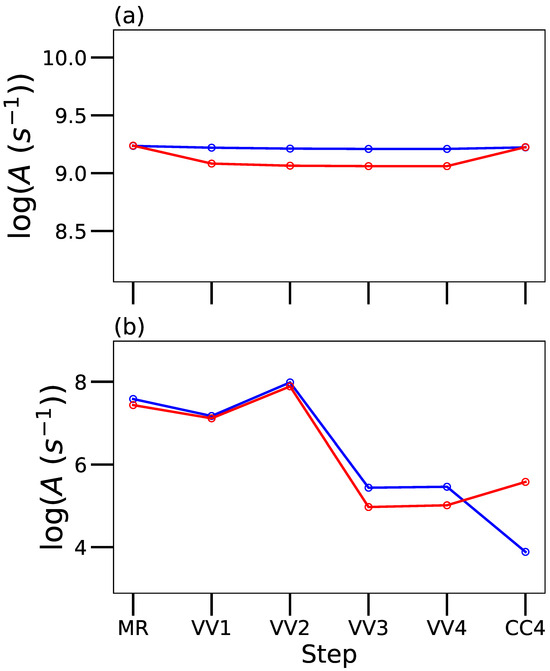
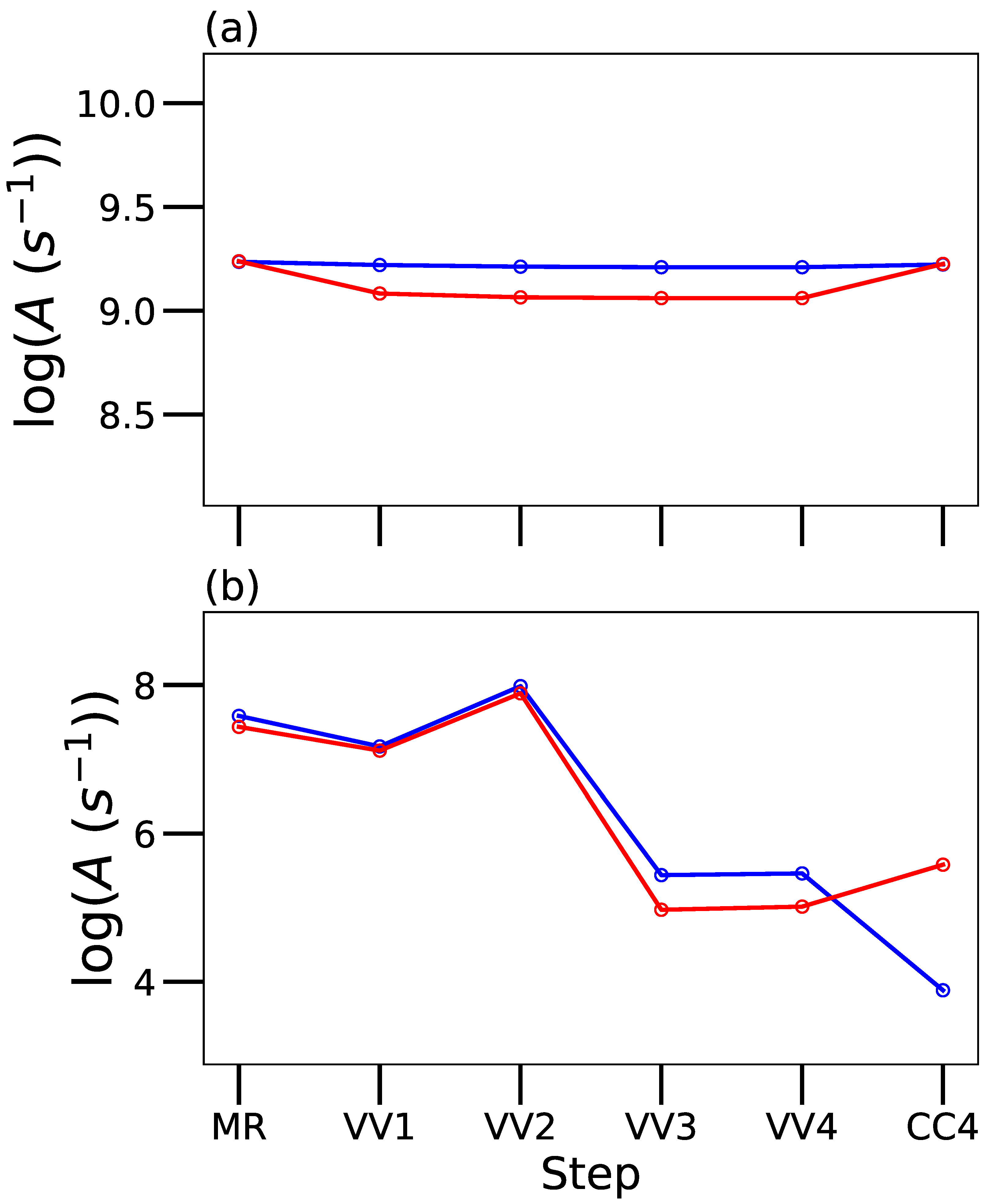
Convergence of the MCDHF-RCI level energies and A-values are illustrated in two examples shown in Figure 2 and Figure 3, respectively, where the different calculation steps are labeled as follows: MR (multireference), VV1 (valence–valence with one correlation layer), VV2 (valence–valence with two correlation layers), etc., up to CC4 (valence–valence, core–valence and core–core with four correlation layers). In Figure 2, one can see that, for both levels, i.e., 5d^{4 5}D₁ at $E=4311.2$ cm⁻¹ [3] (in Panel (a)) and 5d³(⁴F)6s ⁵F₂ at $E=73,848.7$ cm⁻¹ [3] (in Panel (b)), the MCDHF-RCI value converges to the experimental value [3] at the final step, although differently. In Figure 3, the A-values are plotted in a logarithmic scale in the Babushkin (blue line and symbols) and Coulomb (red line and symbols) gauges. In Panel (a), the case of the 5d^{4 5}D₀− 5d³(⁴F)6p ³${\mathrm{D}}_1^o$ transition is shown, where it converges at the final step. A case (the transition 5d^{4 3}P₂− 5d³(²F)6p ³${\mathrm{D}}_1^o$) of clear divergence is presented in Panel (b), where the A-values in both gauges differ by several orders of magnitude at the final step.

Figure 2. Two examples of MCDHF-RCI energy level convergence, i.e., MCDHF-RCI energy versus MCDHF-RCI calculation step, namely MR (multireference), VV1 (valence–valence with one correlation layer), VV2 (valence–valence with 2 correlation layers), etc., up to CC4 (valence–valence, core–valence and core–core with 4 correlation layers). EXP stands for the experimental value of Azarov et al. [3]. Panel (a): 5d^{4 5}D₁ at $E=4311.2$ cm⁻¹ [3]. Panel (b): 5d³(⁴F)6s⁵F₂ at $E=73,848.7$ cm⁻¹ [3]. In both examples, the MCDHF-RCI value converges to the experimental value at the CC4 step, although differently.

Figure 3. Two examples of MCDHF-RCI A-value convergence, i.e., MCDHF-RCI A-value in Babushkin (blue) and Coulomb (red) gauges versus MCDHF-RCI calculation step, namely MR (multireference), VV1 (valence–valence with one correlation layer), VV2 (valence–valence with 2 correlation layers), etc., up to CC4 (valence–valence, core–valence and core–core with 4 correlation layers). Panel (a): 5d^{4 5}D₀− 5d³(⁴F)6p³${\mathrm{D}}_1^o$ transition at $\lambda =705.284$ Å; here it converges at the CC4 step. Panel (b): 5d^{4 3}P₂− 5d³(²F)6p ³${\mathrm{D}}_1^o$ transition at $\lambda =631.706$ Å; here it clearly diverges at the CC4 step.

3. Results and Discussions

Table 2 presents our two sets of calculated energy levels, HFR and MCDHF-RCI, in conjunction with the experimental values of Azarov et al. [3]. Since our focus was on transition probabilities, the table excludes the few unobserved levels that lie between the experimentally established ones. In addition, we include the $LS$-coupling compositions from our HFR model, highlighting the two most significant components. These results indicate that many levels exhibit strong mixing, with purities of 50% or less, most notably in the odd parity. These eigenvector compositions are very similar to those of Azarov et al. [3] and to those obtained in our MCDHF-RCI calculation using the $JJ$-to-$LS$-coupling transformation routine jj2lsj [14]. The latter helps with the level matching between our MCDHF-RCI calculation and the other two sets of levels. In addition, one can see that the mean deviation with respect to the experimental values [3] of our MCDHF-RCI calculation is 3078 cm⁻¹, which represents a relative deviation of 3%.

Table 2. Comparison between experimental, HFR and MCDHF-RCI energy levels in Os V.

i	${\mathit{E}}_{\mathit{Exp}}$ (a)	${\mathit{E}}_{\mathit{HFR}}$ (b)	$\mathbf{\Delta }{\mathit{E}}_{\mathit{HFR}}$ (c)	${\mathit{E}}_{\mathit{RCI}}$ (d)	$\mathbf{\Delta }{\mathit{E}}_{\mathit{RCI}}$ (e)	J	$\mathit{LS}$-Coupling Composition (f)
	(cm−1)	(cm−1)	(cm−1)	(cm−1)	(cm−1)
1	0	0	0	0	0	0	$64\%5{\mathrm{d}}^{4 5}\mathrm{D}+18\%5{\mathrm{d}}^{4 3}\mathrm{P}$
2	4311.2	4280	−31	3959	−352	1	$84\%5{\mathrm{d}}^{4 5}\mathrm{D}+9\%5{\mathrm{d}}^{4 3}\mathrm{P}$
3	8083	8031	−52	7573	−510	2	$92\%5{\mathrm{d}}^{4 5}\mathrm{D}+3\%5{\mathrm{d}}^{4 3}\mathrm{P}$
4	11,018.5	10,930	−89	10,574	−445	3	$87\%5{\mathrm{d}}^{4 5}\mathrm{D}+4\%5{\mathrm{d}}^{4 3}\mathrm{D}$
5	12,966.1	12,856	−110	12,869	−97	4	$69\%5{\mathrm{d}}^{4 5}\mathrm{D}+16\%5{\mathrm{d}}^{4 3}\mathrm{F}$
6	18,364.2	18,452	88	18,824	460	0	$35\%5{\mathrm{d}}^{4 5}\mathrm{D}+32\%5{\mathrm{d}}^{4 3}\mathrm{P}$
7	20,373.8	20,498	124	21,880	1506	4	$57\%5{\mathrm{d}}^{4 3}\mathrm{H}+15\%5{\mathrm{d}}^{4 5}\mathrm{D}$
8	23,942.3	24,090	148	25,462	1520	3	$61\%5{\mathrm{d}}^{4 3}\mathrm{G}+14\%5{\mathrm{d}}^{4 3}\mathrm{F}$
9	24,400.9	24,505	104	25,846	1445	2	$48\%5{\mathrm{d}}^{4 3}\mathrm{F}+19\%5{\mathrm{d}}^{4 3}\mathrm{F}$
10	24,679.7	24,714	34	25,468	788	1	$53\%5{\mathrm{d}}^{4 3}\mathrm{P}+22\%5{\mathrm{d}}^{4 3}\mathrm{P}$
11	25,343.9	25,442	98	27,258	1914	5	$77\%5{\mathrm{d}}^{4 3}\mathrm{H}+23\%5{\mathrm{d}}^{4 3}\mathrm{G}$
12	27,669.2	27,716	47	29,896	2227	6	$75\%5{\mathrm{d}}^{4 3}\mathrm{H}+25\%5{\mathrm{d}}^{4 1}\mathrm{I}$
13	29,844.2	29,965	121	31,419	1575	4	$51\%5{\mathrm{d}}^{4 3}\mathrm{G}+22\%5{\mathrm{d}}^{4 3}\mathrm{H}$
14	30,247.3	30,416	169	31,617	1370	2	$44\%5{\mathrm{d}}^{4 3}\mathrm{P}+38\%5{\mathrm{d}}^{4 3}\mathrm{D}$
15	31,788.2	31,912	124	33,308	1520	4	$37\%5{\mathrm{d}}^{4 3}\mathrm{F}+19\%5{\mathrm{d}}^{4 1}\mathrm{G}$
16	32,171.8	32,433	261	34,025	1853	3	$52\%5{\mathrm{d}}^{4 3}\mathrm{F}+30\%5{\mathrm{d}}^{4 3}\mathrm{D}$
17	34,704.5	34,840	136	36,211	1507	3	$43\%5{\mathrm{d}}^{4 3}\mathrm{D}+26\%5{\mathrm{d}}^{4 3}\mathrm{G}$
18	36,307.1	36,345	38	37,840	1533	2	$22\%5{\mathrm{d}}^{4 1}\mathrm{D}+22\%5{\mathrm{d}}^{4 3}\mathrm{P}$
19	37,015.5	37,028	13	38,840	1825	5	$76\%5{\mathrm{d}}^{4 3}\mathrm{G}+23\%5{\mathrm{d}}^{4 3}\mathrm{H}$
20	38,535.8	38,818	282	40,212	1676	1	$87\%5{\mathrm{d}}^{4 3}\mathrm{D}+7\%5{\mathrm{d}}^{4 3}\mathrm{P}$
21	39,283.5	39,335	52	42,140	2857	6	$75\%5{\mathrm{d}}^{4 1}\mathrm{I}+25\%5{\mathrm{d}}^{4 3}\mathrm{H}$
22	43,779.4	43,880	101	46,099	2320	4	$44\%5{\mathrm{d}}^{4 1}\mathrm{G}+29\%5{\mathrm{d}}^{4 3}\mathrm{F}$
23	43,959.7	44,022	62	46,241	2281	2	$33\%5{\mathrm{d}}^{4 3}\mathrm{P}+26\%5{\mathrm{d}}^{4 3}\mathrm{D}$
24	46,548.9	46,775	226	49,264	2715	3	$62\%5{\mathrm{d}}^{4 1}\mathrm{F}+20\%5{\mathrm{d}}^{4 3}\mathrm{D}$
25	49,999.5	49,915	−85	52,788	2789	2	$57\%5{\mathrm{d}}^{4 3}\mathrm{P}+15\%5{\mathrm{d}}^{4 3}\mathrm{F}$
26	53,794.8	53,442	−353	56,471	2676	4	$64\%5{\mathrm{d}}^{4 3}\mathrm{F}+27\%5{\mathrm{d}}^{4 1}\mathrm{G}$
27	55,042.9	55,146	103	58,016	2973	2	$37\%5{\mathrm{d}}^{4 3}\mathrm{F}+26\%5{\mathrm{d}}^{4 3}\mathrm{F}$
28	55,872	55,855	−17	58,971	3099	3	$63\%5{\mathrm{d}}^{4 3}\mathrm{F}+18\%5{\mathrm{d}}^{4 1}\mathrm{F}$
29	55,987.5	56,001	14	58,986	2999	1	$60\%5{\mathrm{d}}^{4 3}\mathrm{P}+35\%5{\mathrm{d}}^{4 3}\mathrm{P}$
30	59,575.9	59,541	−35	63,443	3867	4	$49\%5{\mathrm{d}}^{4 1}\mathrm{G}+24\%5{\mathrm{d}}^{4 1}\mathrm{G}$
31	71,190.4	71,150	−40	71,302	112	1	$88\%5{\mathrm{d}}^{3}6\mathrm{s}{{(}^4\mathrm{F})}^5\mathrm{F}+6\%5{\mathrm{d}}^{3}6\mathrm{s}{{(}^2\mathrm{D})}^3\mathrm{D}$
32	73,848.7	73,863	14	73,863	14	2	$80\%5{\mathrm{d}}^{3}6\mathrm{s}{{(}^4\mathrm{F})}^5\mathrm{F}+7\%5{\mathrm{d}}^{4 1}\mathrm{D}$
33	78,168.3	78,183	15	78,097	−71	3	$93\%5{\mathrm{d}}^{3}6\mathrm{s}{{(}^4\mathrm{F})}^5\mathrm{F}+2\%5{\mathrm{d}}^{3}6\mathrm{s}{{(}^2\mathrm{D})}^3\mathrm{D}$
34	82,424.4	82,457	33	82,431	7	4	$90\%5{\mathrm{d}}^{3}6\mathrm{s}{{(}^4\mathrm{F})}^5\mathrm{F}+7\%5{\mathrm{d}}^{3}6\mathrm{s}{{(}^2\mathrm{G})}^3\mathrm{G}$
35	85,659.4	85,750	91	86,776	1117	2	$38\%5{\mathrm{d}}^{3}6\mathrm{s}{{(}^4\mathrm{P})}^5\mathrm{P}+21\%5{\mathrm{d}}^{3}6\mathrm{s}{{(}^2\mathrm{P})}^3\mathrm{P}$
36	85,963.9	86,049	85	86,280	316	5	$75\%5{\mathrm{d}}^{3}6\mathrm{s}{{(}^4\mathrm{F})}^5\mathrm{F}+21\%5{\mathrm{d}}^{3}6\mathrm{s}{{(}^2\mathrm{G})}^3\mathrm{G}$
37	87,332.4	87,405	73	88,082	750	1	$76\%5{\mathrm{d}}^{3}6\mathrm{s}{{(}^4\mathrm{P})}^5\mathrm{P}+20\%5{\mathrm{d}}^{3}6\mathrm{s}{{(}^2\mathrm{P})}^3\mathrm{P}$
38	89,238.8	89,265	26	90,456	1217	2	$62\%5{\mathrm{d}}^{3}6\mathrm{s}{{(}^4\mathrm{F})}^3\mathrm{F}+27\%5{\mathrm{d}}^{3}6\mathrm{s}{{(}^4\mathrm{P})}^5\mathrm{P}$
39	92,183.7	92,233	49	93,738	1554	3	$46\%5{\mathrm{d}}^{3}6\mathrm{s}{{(}^2\mathrm{G})}^3\mathrm{G}+44\%5{\mathrm{d}}^{3}6\mathrm{s}{{(}^4\mathrm{F})}^3\mathrm{F}$
40	93,810.8	93,772	−39	95,864	2053	4	$42\%5{\mathrm{d}}^{3}6\mathrm{s}{{(}^2\mathrm{H})}^3\mathrm{H}+31\%5{\mathrm{d}}^{3}6\mathrm{s}{{(}^2\mathrm{G})}^3\mathrm{G}$
41	94,638.7	94,584	−55	95,213	574	3	$90\%5{\mathrm{d}}^{3}6\mathrm{s}{{(}^4\mathrm{P})}^5\mathrm{P}+4\%5{\mathrm{d}}^{3}6\mathrm{s}{{(}^2\mathrm{D})}^3\mathrm{D}$
42	97,477	97,604	127	99,443	1966	5	$47\%5{\mathrm{d}}^{3}6\mathrm{s}{{(}^2\mathrm{H})}^3\mathrm{H}+24\%5{\mathrm{d}}^{3}6\mathrm{s}{{(}^2\mathrm{G})}^3\mathrm{G}$
43	98,874	99,112	238	100,915	2041	4	$40\%5{\mathrm{d}}^{3}6\mathrm{s}{{(}^2\mathrm{G})}^3\mathrm{G}+36\%5{\mathrm{d}}^{3}6\mathrm{s}{{(}^2\mathrm{G})}^1\mathrm{G}$
44	99,046.4	99,039	−7	100,512	1466	3	$46\%5{\mathrm{d}}^{3}6\mathrm{s}{{(}^2\mathrm{G})}^3\mathrm{G}+45\%5{\mathrm{d}}^{3}6\mathrm{s}{{(}^4\mathrm{F})}^3\mathrm{F}$
45	101,269.7	101,515	245	102,576	1306	2	$28\%5{\mathrm{d}}^{3}6\mathrm{s}{{(}^2\mathrm{D})}^3\mathrm{D}+28\%5{\mathrm{d}}^{3}6\mathrm{s}{{(}^4\mathrm{P})}^5\mathrm{P}$
46	102,359.2	102,204	−155	104,201	1842	4	$53\%5{\mathrm{d}}^{3}6\mathrm{s}{{(}^4\mathrm{F})}^3\mathrm{F}+41\%5{\mathrm{d}}^{3}6\mathrm{s}{{(}^2\mathrm{H})}^3\mathrm{H}$
47	104,990.6	105,069	78	107,586	2595	6	$100\%5{\mathrm{d}}^{3}6\mathrm{s}{{(}^2\mathrm{H})}^3\mathrm{H}$
48	107,300.6	107,394	93	109,253	1952	2	$46\%5{\mathrm{d}}^{3}6\mathrm{s}{{(}^4\mathrm{P})}^3\mathrm{P}+15\%5{\mathrm{d}}^{3}6\mathrm{s}{{(}^2\mathrm{D})}^3\mathrm{D}$
49	107,899.1	107,818	−81	110,179	2280	5	$50\%5{\mathrm{d}}^{3}6\mathrm{s}{{(}^2\mathrm{H})}^3\mathrm{H}+28\%5{\mathrm{d}}^{3}6\mathrm{s}{{(}^2\mathrm{G})}^3\mathrm{G}$
50	108,078.7	108,463	384	109,711	1632	3	$83\%5{\mathrm{d}}^{3}6\mathrm{s}{{(}^2\mathrm{D})}^3\mathrm{D}+7\%5{\mathrm{d}}^{3}6\mathrm{s}{{(}^2\mathrm{D})}^3\mathrm{D}$
51	112,647.5	112,611	−37	115,534	2887	5	$70\%5{\mathrm{d}}^{3}6\mathrm{s}{{(}^2\mathrm{H})}^1\mathrm{H}+27\%5{\mathrm{d}}^{3}6\mathrm{s}{{(}^2\mathrm{G})}^3\mathrm{G}$
52	112,937.4	112,961	24	115,711	2774	3	$87\%5{\mathrm{d}}^{3}6\mathrm{s}{{(}^2\mathrm{F})}^3\mathrm{F}+6\%5{\mathrm{d}}^{3}6\mathrm{s}{{(}^2\mathrm{D})}^3\mathrm{D}$
53	113,528.1	113,703	175	116,092	2564	4	$80\%5{\mathrm{d}}^{3}6\mathrm{s}{{(}^2\mathrm{F})}^3\mathrm{F}+9\%5{\mathrm{d}}^{3}6\mathrm{s}{{(}^2\mathrm{G})}^3\mathrm{G}$
54	114,015.2	114,175	160	116,474	2459	2	$42\%5{\mathrm{d}}^{3}6\mathrm{s}{{(}^4\mathrm{P})}^3\mathrm{P}+31\%5{\mathrm{d}}^{3}6\mathrm{s}{{(}^2\mathrm{F})}^3\mathrm{F}$
55	114,903.9	114,912	8	117,174	2270	4	$51\%5{\mathrm{d}}^{3}6\mathrm{s}{{(}^2\mathrm{G})}^1\mathrm{G}+16\%5{\mathrm{d}}^{3}6\mathrm{s}{{(}^4\mathrm{F})}^3\mathrm{F}$
56	120,656.4	120,770	114	124,264	3608	3	$82\%5{\mathrm{d}}^{3}6\mathrm{s}{{(}^2\mathrm{F})}^1\mathrm{F}+10\%5{\mathrm{d}}^{3}6\mathrm{s}{{(}^2\mathrm{D})}^3\mathrm{D}$
57	133,008.9	132,798	−211	136,238	3229	2	$67\%5{\mathrm{d}}^{3}6\mathrm{s}{{(}^2\mathrm{D})}^3\mathrm{D}+19\%5{\mathrm{d}}^{3}6\mathrm{s}{{(}^2\mathrm{D})}^3\mathrm{D}$
58	141,786.5	141,463	−324	144,751	2965	1	$42\%5{\mathrm{d}}^{3}6\mathrm{p}{{(}^4\mathrm{F})}^3{\mathrm{D}}^{\mathrm{o}}+35\%5{\mathrm{d}}^{3}6\mathrm{p}{{(}^4\mathrm{F})}^5{\mathrm{F}}^{\mathrm{o}}$
59	145,171.8	145,482	310	147,879	2707	3	$75\%5{\mathrm{d}}^{3}6\mathrm{p}{{(}^4\mathrm{F})}^5{\mathrm{G}}^{\mathrm{o}}+10\%5{\mathrm{d}}^{3}6\mathrm{p}{{(}^4\mathrm{F})}^3{\mathrm{F}}^{\mathrm{o}}$
60	146,735.2	146,868	133	149,510	2775	2	$33\%5{\mathrm{d}}^{3}6\mathrm{p}{{(}^4\mathrm{F})}^5{\mathrm{F}}^{\mathrm{o}}+33\%5{\mathrm{d}}^{3}6\mathrm{p}{{(}^4\mathrm{F})}^3{\mathrm{D}}^{\mathrm{o}}$
61	150,490.2	150,787	297	153,504	3014	4	$54\%5{\mathrm{d}}^{3}6\mathrm{p}{{(}^4\mathrm{F})}^5{\mathrm{G}}^{\mathrm{o}}+12\%5{\mathrm{d}}^{3}6\mathrm{p}{{(}^4\mathrm{F})}^3{\mathrm{G}}^{\mathrm{o}}$
62	152,747.8	153,266	518	156,166	3418	1	$34\%5{\mathrm{d}}^{3}6\mathrm{p}{{(}^4\mathrm{P})}^5{\mathrm{D}}^{\mathrm{o}}+14\%5{\mathrm{d}}^{3}6\mathrm{p}{{(}^2\mathrm{P})}^3{\mathrm{D}}^{\mathrm{o}}$
63	153,253.8	152,961	−293	156,159	2905	3	$30\%5{\mathrm{d}}^{3}6\mathrm{p}{{(}^4\mathrm{F})}^5{\mathrm{F}}^{\mathrm{o}}+27\%5{\mathrm{d}}^{3}6\mathrm{p}{{(}^4\mathrm{F})}^5{\mathrm{D}}^{\mathrm{o}}$
64	153,509.7	153,650	140	156,866	3356	2	$22\%5{\mathrm{d}}^{3}6\mathrm{p}{{(}^4\mathrm{P})}^5{\mathrm{D}}^{\mathrm{o}}+13\%5{\mathrm{d}}^{3}6\mathrm{p}{{(}^2\mathrm{P})}^3{\mathrm{D}}^{\mathrm{o}}$
65	153,709.2	154,063	354	157,436	3727	5	$20\%5{\mathrm{d}}^{3}6\mathrm{p}{{(}^4\mathrm{F})}^5{\mathrm{G}}^{\mathrm{o}}+13\%5{\mathrm{d}}^{3}6\mathrm{p}{{(}^2\mathrm{G})}^3{\mathrm{G}}^{\mathrm{o}}$
66	157,473.4	157,022	−451	160,910	3437	4	$35\%5{\mathrm{d}}^{3}6\mathrm{p}{{(}^4\mathrm{F})}^5{\mathrm{D}}^{\mathrm{o}}+15\%5{\mathrm{d}}^{3}6\mathrm{p}{{(}^2\mathrm{G})}^3{\mathrm{F}}^{\mathrm{o}}$
67	157,712.2	157,476	−236	160,572	2860	1	$23\%5{\mathrm{d}}^{3}6\mathrm{p}{{(}^4\mathrm{P})}^5{\mathrm{P}}^{\mathrm{o}}+23\%5{\mathrm{d}}^{3}6\mathrm{p}{{(}^4\mathrm{F})}^5{\mathrm{F}}^{\mathrm{o}}$
68	159,602.6	159,334	−269	162,747	3144	1	$35\%5{\mathrm{d}}^{3}6\mathrm{p}{{(}^4\mathrm{F})}^5{\mathrm{D}}^{\mathrm{o}}+17\%5{\mathrm{d}}^{3}6\mathrm{p}{{(}^4\mathrm{P})}^5{\mathrm{P}}^{\mathrm{o}}$
69	159,898	160,134	236	162,918	3020	3	$33\%5{\mathrm{d}}^{3}6\mathrm{p}{{(}^4\mathrm{F})}^3{\mathrm{G}}^{\mathrm{o}}+15\%5{\mathrm{d}}^{3}6\mathrm{p}{{(}^4\mathrm{F})}^5{\mathrm{D}}^{\mathrm{o}}$
70	160,232.9	160,325	92	162,789	2556	2	$36\%5{\mathrm{d}}^{3}6\mathrm{p}{{(}^4\mathrm{F})}^5{\mathrm{F}}^{\mathrm{o}}+30\%5{\mathrm{d}}^{3}6\mathrm{p}{{(}^4\mathrm{F})}^5{\mathrm{D}}^{\mathrm{o}}$
71	161,011.3	161,410	399	164,628	3617	4	$39\%5{\mathrm{d}}^{3}6\mathrm{p}{{(}^2\mathrm{G})}^3{\mathrm{H}}^{\mathrm{o}}+25\%5{\mathrm{d}}^{3}6\mathrm{p}{{(}^4\mathrm{F})}^5{\mathrm{G}}^{\mathrm{o}}$
72	163,004	163,092	88	166,316	3312	3	$19\%5{\mathrm{d}}^{3}6\mathrm{p}{{(}^4\mathrm{P})}^5{\mathrm{D}}^{\mathrm{o}}+14\%5{\mathrm{d}}^{3}6\mathrm{p}{{(}^4\mathrm{F})}^5{\mathrm{F}}^{\mathrm{o}}$
73	163,674.8	163,856	181	167,603	3928	5	$36\%5{\mathrm{d}}^{3}6\mathrm{p}{{(}^4\mathrm{F})}^5{\mathrm{G}}^{\mathrm{o}}+31\%5{\mathrm{d}}^{3}6\mathrm{p}{{(}^2\mathrm{H})}^3{\mathrm{I}}^{\mathrm{o}}$
74	163,890.8	163,766	−125	167,063	3172	2	$46\%5{\mathrm{d}}^{3}6\mathrm{p}{{(}^4\mathrm{P})}^5{\mathrm{P}}^{\mathrm{o}}+18\%5{\mathrm{d}}^{3}6\mathrm{p}{{(}^4\mathrm{P})}^3{\mathrm{P}}^{\mathrm{o}}$
75	164,663.2	164,415	−248	167,635	2972	3	$31\%5{\mathrm{d}}^{3}6\mathrm{p}{{(}^4\mathrm{F})}^5{\mathrm{F}}^{\mathrm{o}}+15\%5{\mathrm{d}}^{3}6\mathrm{p}{{(}^4\mathrm{P})}^5{\mathrm{D}}^{\mathrm{o}}$
76	164,811.1	164,684	−127	168,007	3196	4	$34\%5{\mathrm{d}}^{3}6\mathrm{p}{{(}^4\mathrm{F})}^5{\mathrm{F}}^{\mathrm{o}}+18\%5{\mathrm{d}}^{3}6\mathrm{p}{{(}^2\mathrm{H})}^3{\mathrm{H}}^{\mathrm{o}}$
77	165,257.7	165,116	−142	167,827	2569	1	$40\%5{\mathrm{d}}^{3}6\mathrm{p}{{(}^4\mathrm{F})}^5{\mathrm{D}}^{\mathrm{o}}+21\%5{\mathrm{d}}^{3}6\mathrm{p}{{(}^4\mathrm{F})}^3{\mathrm{D}}^{\mathrm{o}}$
78	167,207.2	166,913	−294	171,316	4109	4	$23\%5{\mathrm{d}}^{3}6\mathrm{p}{{(}^2\mathrm{G})}^3{\mathrm{H}}^{\mathrm{o}}+22\%5{\mathrm{d}}^{3}6\mathrm{p}{{(}^4\mathrm{F})}^5{\mathrm{D}}^{\mathrm{o}}$
79	167,420.9	167,823	402	171,096	3675	1	$27\%5{\mathrm{d}}^{3}6\mathrm{p}{{(}^4\mathrm{P})}^5{\mathrm{D}}^{\mathrm{o}}+21\%5{\mathrm{d}}^{3}6\mathrm{p}{{(}^2\mathrm{P})}^3{\mathrm{D}}^{\mathrm{o}}$
80	167,627	167,896	269	171,020	3393	3	$35\%5{\mathrm{d}}^{3}6\mathrm{p}{{(}^4\mathrm{F})}^3{\mathrm{G}}^{\mathrm{o}}+13\%5{\mathrm{d}}^{3}6\mathrm{p}{{(}^4\mathrm{F})}^5{\mathrm{D}}^{\mathrm{o}}$
81	168,225.4	168,118	−107	171,152	2927	5	$35\%5{\mathrm{d}}^{3}6\mathrm{p}{{(}^4\mathrm{F})}^5{\mathrm{G}}^{\mathrm{o}}+25\%5{\mathrm{d}}^{3}6\mathrm{p}{{(}^4\mathrm{F})}^5{\mathrm{F}}^{\mathrm{o}}$
82	169,095	169,009	−86	171,955	2860	2	$31\%5{\mathrm{d}}^{3}6\mathrm{p}{{(}^4\mathrm{F})}^5{\mathrm{D}}^{\mathrm{o}}+23\%5{\mathrm{d}}^{3}6\mathrm{p}{{(}^4\mathrm{F})}^3{\mathrm{D}}^{\mathrm{o}}$
83	169,759	169,700	−59	172,860	3101	6	$55\%5{\mathrm{d}}^{3}6\mathrm{p}{{(}^4\mathrm{F})}^5{\mathrm{G}}^{\mathrm{o}}+22\%5{\mathrm{d}}^{3}6\mathrm{p}{{(}^2\mathrm{G})}^3{\mathrm{H}}^{\mathrm{o}}$
84	170,217.6	170,252	34	173,481	3263	2	$35\%5{\mathrm{d}}^{3}6\mathrm{p}{{(}^4\mathrm{F})}^3{\mathrm{F}}^{\mathrm{o}}+9\%5{\mathrm{d}}^{3}6\mathrm{p}{{(}^4\mathrm{P})}^5{\mathrm{D}}^{\mathrm{o}}$
85	171,199	171,066	−133	174,325	3126	3	$26\%5{\mathrm{d}}^{3}6\mathrm{p}{{(}^4\mathrm{P})}^5{\mathrm{P}}^{\mathrm{o}}+18\%5{\mathrm{d}}^{3}6\mathrm{p}{{(}^4\mathrm{F})}^3{\mathrm{F}}^{\mathrm{o}}$
86	171,780.3	171,460	−320	175,771	3991	1	$34\%5{\mathrm{d}}^{3}6\mathrm{p}{{(}^2\mathrm{P})}^3{\mathrm{D}}^{\mathrm{o}}+22\%5{\mathrm{d}}^{3}6\mathrm{p}{{(}^4\mathrm{P})}^5{\mathrm{P}}^{\mathrm{o}}$
87	172,485.7	172,239	−247	175,747	3261	3	$16\%5{\mathrm{d}}^{3}6\mathrm{p}{{(}^4\mathrm{P})}^5{\mathrm{P}}^{\mathrm{o}}+13\%5{\mathrm{d}}^{3}6\mathrm{p}{{(}^4\mathrm{F})}^3{\mathrm{D}}^{\mathrm{o}}$
88	172,687.5	172,871	184	175,622	2935	4	$48\%5{\mathrm{d}}^{3}6\mathrm{p}{{(}^4\mathrm{F})}^3{\mathrm{G}}^{\mathrm{o}}+32\%5{\mathrm{d}}^{3}6\mathrm{p}{{(}^4\mathrm{F})}^5{\mathrm{F}}^{\mathrm{o}}$
89	172,725.3	172,712	−13	177,606	4881	6	$34\%5{\mathrm{d}}^{3}6\mathrm{p}{{(}^2\mathrm{H})}^3{\mathrm{H}}^{\mathrm{o}}+27\%5{\mathrm{d}}^{3}6\mathrm{p}{{(}^2\mathrm{H})}^3{\mathrm{I}}^{\mathrm{o}}$
90	173,052.9	173,214	161	176,415	3362	2	$18\%5{\mathrm{d}}^{3}6\mathrm{p}{{(}^4\mathrm{P})}^5{\mathrm{P}}^{\mathrm{o}}+12\%5{\mathrm{d}}^{3}6\mathrm{p}{{(}^4\mathrm{P})}^5{\mathrm{D}}^{\mathrm{o}}$
91	173,239	172,995	−244	177,782	4543	5	$42\%5{\mathrm{d}}^{3}6\mathrm{p}{{(}^2\mathrm{H})}^3{\mathrm{H}}^{\mathrm{o}}+27\%5{\mathrm{d}}^{3}6\mathrm{p}{{(}^2\mathrm{H})}^3{\mathrm{G}}^{\mathrm{o}}$
92	174,500.2	174,622	122	177,954	3454	4	$33\%5{\mathrm{d}}^{3}6\mathrm{p}{{(}^4\mathrm{F})}^3{\mathrm{F}}^{\mathrm{o}}+14\%5{\mathrm{d}}^{3}6\mathrm{p}{{(}^2\mathrm{G})}^3{\mathrm{F}}^{\mathrm{o}}$
93	174,562.9	174,596	33	177,895	3332	3	$24\%5{\mathrm{d}}^{3}6\mathrm{p}{{(}^4\mathrm{P})}^5{\mathrm{D}}^{\mathrm{o}}+19\%5{\mathrm{d}}^{3}6\mathrm{p}{{(}^2\mathrm{G})}^3{\mathrm{F}}^{\mathrm{o}}$
94	175,348.5	175,771	423	178,736	3388	1	$47\%5{\mathrm{d}}^{3}6\mathrm{p}{{(}^4\mathrm{P})}^3{\mathrm{P}}^{\mathrm{o}}+15\%5{\mathrm{d}}^{3}6\mathrm{p}{{(}^2\mathrm{P})}^3{\mathrm{S}}^{\mathrm{o}}$
95	175,382.2	175,670	288	179,196	3814	2	$23\%5{\mathrm{d}}^{3}6\mathrm{p}{{(}^2\mathrm{D})}^3{\mathrm{D}}^{\mathrm{o}}+19\%5{\mathrm{d}}^{3}6\mathrm{p}{{(}^2\mathrm{D})}^3{\mathrm{P}}^{\mathrm{o}}$
96	177,191.4	177,350	159	181,276	4085	4	$46\%5{\mathrm{d}}^{3}6\mathrm{p}{{(}^2\mathrm{G})}^3{\mathrm{G}}^{\mathrm{o}}+18\%5{\mathrm{d}}^{3}6\mathrm{p}{{(}^2\mathrm{G})}^3{\mathrm{F}}^{\mathrm{o}}$
97	177,270.2	177,468	198	181,584	4314	3	$19\%5{\mathrm{d}}^{3}6\mathrm{p}{{(}^2\mathrm{F})}^3{\mathrm{G}}^{\mathrm{o}}+16\%5{\mathrm{d}}^{3}6\mathrm{p}{{(}^2\mathrm{F})}^3{\mathrm{F}}^{\mathrm{o}}$
98	177,548.6	177,581	32	181,460	3911	5	$36\%5{\mathrm{d}}^{3}6\mathrm{p}{{(}^2\mathrm{G})}^3{\mathrm{H}}^{\mathrm{o}}+22\%5{\mathrm{d}}^{3}6\mathrm{p}{{(}^4\mathrm{F})}^5{\mathrm{F}}^{\mathrm{o}}$
99	177,721	177,626	−95	182,216	4495	2	$33\%5{\mathrm{d}}^{3}6\mathrm{p}{{(}^2\mathrm{F})}^3{\mathrm{F}}^{\mathrm{o}}+19\%5{\mathrm{d}}^{3}6\mathrm{p}{{(}^2\mathrm{F})}^1{\mathrm{D}}^{\mathrm{o}}$
100	177,946.2	178,219	273	182,508	4562	5	$28\%5{\mathrm{d}}^{3}6\mathrm{p}{{(}^4\mathrm{F})}^3{\mathrm{G}}^{\mathrm{o}}+26\%5{\mathrm{d}}^{3}6\mathrm{p}{{(}^2\mathrm{G})}^3{\mathrm{G}}^{\mathrm{o}}$
101	178,719.7	178,751	31	183,123	4403	3	$18\%5{\mathrm{d}}^{3}6\mathrm{p}{{(}^2\mathrm{D})}^3{\mathrm{F}}^{\mathrm{o}}+15\%5{\mathrm{d}}^{3}6\mathrm{p}{{(}^2\mathrm{F})}^3{\mathrm{G}}^{\mathrm{o}}$
102	178,784.2	178,960	176	183,393	4609	4	$22\%5{\mathrm{d}}^{3}6\mathrm{p}{{(}^2\mathrm{F})}^3{\mathrm{F}}^{\mathrm{o}}+20\%5{\mathrm{d}}^{3}6\mathrm{p}{{(}^2\mathrm{F})}^3{\mathrm{G}}^{\mathrm{o}}$
103	179,411	179,798	387	183,291	3880	2	$24\%5{\mathrm{d}}^{3}6\mathrm{p}{{(}^2\mathrm{G})}^3{\mathrm{F}}^{\mathrm{o}}+16\%5{\mathrm{d}}^{3}6\mathrm{p}{{(}^2\mathrm{P})}^1{\mathrm{D}}^{\mathrm{o}}$
104	179,935.6	180,302	366	184,036	4100	2	$22\%5{\mathrm{d}}^{3}6\mathrm{p}{{(}^4\mathrm{P})}^3{\mathrm{D}}^{\mathrm{o}}+18\%5{\mathrm{d}}^{3}6\mathrm{p}{{(}^2\mathrm{P})}^3{\mathrm{D}}^{\mathrm{o}}$
105	181,016.2	180,871	−145	185,377	4361	3	$26\%5{\mathrm{d}}^{3}6\mathrm{p}{{(}^2\mathrm{F})}^3{\mathrm{D}}^{\mathrm{o}}+13\%5{\mathrm{d}}^{3}6\mathrm{p}{{(}^2\mathrm{F})}^3{\mathrm{F}}^{\mathrm{o}}$
106	181,029.4	180,957	−72	184,625	3596	4	$46\%5{\mathrm{d}}^{3}6\mathrm{p}{{(}^4\mathrm{P})}^5{\mathrm{D}}^{\mathrm{o}}+10\%5{\mathrm{d}}^{3}6\mathrm{p}{{(}^2\mathrm{H})}^3{\mathrm{H}}^{\mathrm{o}}$
107	181,634.9	181,676	41	185,592	3957	5	$31\%5{\mathrm{d}}^{3}6\mathrm{p}{{(}^2\mathrm{G})}^3{\mathrm{H}}^{\mathrm{o}}+18\%5{\mathrm{d}}^{3}6\mathrm{p}{{(}^4\mathrm{F})}^5{\mathrm{F}}^{\mathrm{o}}$
108	182,382.9	182,417	34	186,447	4064	4	$28\%5{\mathrm{d}}^{3}6\mathrm{p}{{(}^4\mathrm{P})}^5{\mathrm{D}}^{\mathrm{o}}+22\%5{\mathrm{d}}^{3}6\mathrm{p}{{(}^2\mathrm{G})}^1{\mathrm{G}}^{\mathrm{o}}$
109	182,444.2	182,625	181	186,985	4541	6	$30\%5{\mathrm{d}}^{3}6\mathrm{p}{{(}^2\mathrm{H})}^1{\mathrm{I}}^{\mathrm{o}}+26\%5{\mathrm{d}}^{3}6\mathrm{p}{{(}^2\mathrm{G})}^3{\mathrm{H}}^{\mathrm{o}}$
110	184,080.4	183,992	-88	187,642	3562	3	$15\%5{\mathrm{d}}^{3}6\mathrm{p}{{(}^2\mathrm{G})}^1{\mathrm{F}}^{\mathrm{o}}+15\%5{\mathrm{d}}^{3}6\mathrm{p}{{(}^2\mathrm{H})}^3{\mathrm{G}}^{\mathrm{o}}$
111	184,535	184,376	−159	189,172	4637	5	$40\%5{\mathrm{d}}^{3}6\mathrm{p}{{(}^2\mathrm{G})}^1{\mathrm{H}}^{\mathrm{o}}+18\%5{\mathrm{d}}^{3}6\mathrm{p}{{(}^4\mathrm{F})}^3{\mathrm{G}}^{\mathrm{o}}$
112	184,539.4	184,646	107	188,946	4407	3	$25\%5{\mathrm{d}}^{3}6\mathrm{p}{{(}^2\mathrm{G})}^3{\mathrm{G}}^{\mathrm{o}}+21\%5{\mathrm{d}}^{3}6\mathrm{p}{{(}^2\mathrm{G})}^3{\mathrm{F}}^{\mathrm{o}}$
113	184,571	184,857	286	188,862	4291	2	$51\%5{\mathrm{d}}^{3}6\mathrm{p}{{(}^2\mathrm{G})}^3{\mathrm{F}}^{\mathrm{o}}+10\%5{\mathrm{d}}^{3}6\mathrm{p}{{(}^2\mathrm{P})}^3{\mathrm{D}}^{\mathrm{o}}$
114	184,627	184,450	−177	188,624	3997	4	$18\%5{\mathrm{d}}^{3}6\mathrm{p}{{(}^4\mathrm{F})}^3{\mathrm{F}}^{\mathrm{o}}+14\%5{\mathrm{d}}^{3}6\mathrm{p}{{(}^2\mathrm{H})}^1{\mathrm{G}}^{\mathrm{o}}$
115	185,252.5	185,354	102	188,428	3176	2	$48\%5{\mathrm{d}}^{3}6\mathrm{p}{{(}^4\mathrm{P})}^5{\mathrm{S}}^{\mathrm{o}}+19\%5{\mathrm{d}}^{3}6\mathrm{p}{{(}^4\mathrm{P})}^3{\mathrm{P}}^{\mathrm{o}}$
116	186,310	186,431	121	190,769	4459	3	$25\%5{\mathrm{d}}^{3}6\mathrm{p}{{(}^2\mathrm{H})}^3{\mathrm{G}}^{\mathrm{o}}+14\%5{\mathrm{d}}^{3}6\mathrm{p}{{(}^4\mathrm{P})}^5{\mathrm{D}}^{\mathrm{o}}$
117	186,670.3	186,633	−37	190,577	3907	2	$20\%5{\mathrm{d}}^{3}6\mathrm{p}{{(}^2\mathrm{P})}^3{\mathrm{D}}^{\mathrm{o}}+17\%5{\mathrm{d}}^{3}6\mathrm{p}{{(}^2\mathrm{P})}^1{\mathrm{D}}^{\mathrm{o}}$
118	187,662.9	187,496	−167	192,367	4704	6	$46\%5{\mathrm{d}}^{3}6\mathrm{p}{{(}^2\mathrm{H})}^3{\mathrm{H}}^{\mathrm{o}}+30\%5{\mathrm{d}}^{3}6\mathrm{p}{{(}^2\mathrm{H})}^3{\mathrm{I}}^{\mathrm{o}}$
119	187,919.3	188,311	392	191,774	3855	1	$31\%5{\mathrm{d}}^{3}6\mathrm{p}{{(}^4\mathrm{P})}^3{\mathrm{D}}^{\mathrm{o}}+17\%5{\mathrm{d}}^{3}6\mathrm{p}{{(}^2\mathrm{P})}^3{\mathrm{S}}^{\mathrm{o}}$
120	188,832.6	188,812	−21	192,796	3963	3	$40\%5{\mathrm{d}}^{3}6\mathrm{p}{{(}^4\mathrm{P})}^3{\mathrm{D}}^{\mathrm{o}}+17\%5{\mathrm{d}}^{3}6\mathrm{p}{{(}^4\mathrm{F})}^3{\mathrm{D}}^{\mathrm{o}}$
121	189,915.7	190,131	215	195,185	5269	7	$100\%5{\mathrm{d}}^{3}6\mathrm{p}{{(}^2\mathrm{H})}^3{\mathrm{I}}^{\mathrm{o}}$
122	190,406.8	190,443	36	194,294	3887	2	$25\%5{\mathrm{d}}^{3}6\mathrm{p}{{(}^4\mathrm{P})}^3{\mathrm{D}}^{\mathrm{o}}+19\%5{\mathrm{d}}^{3}6\mathrm{p}{{(}^2\mathrm{D})}^3{\mathrm{D}}^{\mathrm{o}}$
123	191,070.2	190,986	−84	195,541	4471	5	$46\%5{\mathrm{d}}^{3}6\mathrm{p}{{(}^2\mathrm{H})}^1{\mathrm{H}}^{\mathrm{o}}+24\%5{\mathrm{d}}^{3}6\mathrm{p}{{(}^2\mathrm{G})}^3{\mathrm{G}}^{\mathrm{o}}$
124	191,618.3	191,942	324	195,485	3867	4	$63\%5{\mathrm{d}}^{3}6\mathrm{p}{{(}^2\mathrm{D})}^3{\mathrm{F}}^{\mathrm{o}}+6\%5{\mathrm{d}}^{3}6\mathrm{p}{{(}^2\mathrm{F})}^3{\mathrm{G}}^{\mathrm{o}}$
125	193,770.2	193,700	−70	198,621	4851	4	$33\%5{\mathrm{d}}^{3}6\mathrm{p}{{(}^2\mathrm{H})}^3{\mathrm{G}}^{\mathrm{o}}+22\%5{\mathrm{d}}^{3}6\mathrm{p}{{(}^2\mathrm{H})}^1{\mathrm{G}}^{\mathrm{o}}$
126	193,807.7	193,845	37	198,187	4379	3	$17\%5{\mathrm{d}}^{3}6\mathrm{p}{{(}^2\mathrm{D})}^3{\mathrm{D}}^{\mathrm{o}}+12\%5{\mathrm{d}}^{3}6\mathrm{p}{{(}^2\mathrm{P})}^3{\mathrm{D}}^{\mathrm{o}}$
127	194,447.3	194,822	375	199,207	4760	2	$19\%5{\mathrm{d}}^{3}6\mathrm{p}{{(}^2\mathrm{P})}^1{\mathrm{D}}^{\mathrm{o}}+14\%5{\mathrm{d}}^{3}6\mathrm{p}{{(}^2\mathrm{F})}^3{\mathrm{F}}^{\mathrm{o}}$
128	194,539.7	194,533	−7	199,159	4619	5	$30\%5{\mathrm{d}}^{3}6\mathrm{p}{{(}^2\mathrm{H})}^3{\mathrm{G}}^{\mathrm{o}}+21\%5{\mathrm{d}}^{3}6\mathrm{p}{{(}^2\mathrm{G})}^1{\mathrm{H}}^{\mathrm{o}}$
129	195,276	195,342	66	199,881	4605	3	$28\%5{\mathrm{d}}^{3}6\mathrm{p}{{(}^2\mathrm{D})}^3{\mathrm{D}}^{\mathrm{o}}+21\%5{\mathrm{d}}^{3}6\mathrm{p}{{(}^2\mathrm{H})}^3{\mathrm{G}}^{\mathrm{o}}$
130	195,415.5	195,651	236	200,183	4768	6	$42\%5{\mathrm{d}}^{3}6\mathrm{p}{{(}^2\mathrm{G})}^3{\mathrm{H}}^{\mathrm{o}}+38\%5{\mathrm{d}}^{3}6\mathrm{p}{{(}^2\mathrm{H})}^1{\mathrm{I}}^{\mathrm{o}}$
131	195,991	196,330	339	200,858	4867	2	$20\%5{\mathrm{d}}^{3}6\mathrm{p}{{(}^2\mathrm{D})}^3{\mathrm{P}}^{\mathrm{o}}+19\%5{\mathrm{d}}^{3}6\mathrm{p}{{(}^2\mathrm{D})}^1{\mathrm{D}}^{\mathrm{o}}$
132	196,051.8	196,340	288	200,437	4385	1	$40\%5{\mathrm{d}}^{3}6\mathrm{p}{{(}^4\mathrm{P})}^3{\mathrm{S}}^{\mathrm{o}}+25\%5{\mathrm{d}}^{3}6\mathrm{p}{{(}^2\mathrm{D})}^3{\mathrm{P}}^{\mathrm{o}}$
133	196,573.8	196,401	−173	200,803	4229	4	$22\%5{\mathrm{d}}^{3}6\mathrm{p}{{(}^2\mathrm{G})}^1{\mathrm{G}}^{\mathrm{o}}+14\%5{\mathrm{d}}^{3}6\mathrm{p}{{(}^2\mathrm{G})}^3{\mathrm{F}}^{\mathrm{o}}$
134	197,023.3	197,015	−8	201,457	4434	3	$22\%5{\mathrm{d}}^{3}6\mathrm{p}{{(}^2\mathrm{F})}^3{\mathrm{F}}^{\mathrm{o}}+14\%5{\mathrm{d}}^{3}6\mathrm{p}{{(}^2\mathrm{P})}^3{\mathrm{D}}^{\mathrm{o}}$
135	199,242.4	199,629	387	204,541	5299	5	$85\%5{\mathrm{d}}^{3}6\mathrm{p}{{(}^2\mathrm{F})}^3{\mathrm{G}}^{\mathrm{o}}+5\%5{\mathrm{d}}^{3}6\mathrm{p}{{(}^2\mathrm{G})}^1{\mathrm{H}}^{\mathrm{o}}$
136	199,726.5	199,764	38	204,731	5005	4	$32\%5{\mathrm{d}}^{3}6\mathrm{p}{{(}^2\mathrm{F})}^3{\mathrm{F}}^{\mathrm{o}}+28\%5{\mathrm{d}}^{3}6\mathrm{p}{{(}^2\mathrm{F})}^3{\mathrm{G}}^{\mathrm{o}}$
137	199,942.5	200,298	356	204,847	4905	2	$48\%5{\mathrm{d}}^{3}6\mathrm{p}{{(}^2\mathrm{F})}^3{\mathrm{D}}^{\mathrm{o}}+7\%5{\mathrm{d}}^{3}6\mathrm{p}{{(}^2\mathrm{F})}^3{\mathrm{F}}^{\mathrm{o}}$
138	200,274.9	200,717	442	204,683	4408	3	$20\%5{\mathrm{d}}^{3}6\mathrm{p}{{(}^2\mathrm{P})}^3{\mathrm{D}}^{\mathrm{o}}+16\%5{\mathrm{d}}^{3}6\mathrm{p}{{(}^2\mathrm{D})}^1{\mathrm{F}}^{\mathrm{o}}$
139	201,739.2	201,579	−160	207,561	5822	4	$48\%5{\mathrm{d}}^{3}6\mathrm{p}{{(}^2\mathrm{F})}^1{\mathrm{G}}^{\mathrm{o}}+25\%5{\mathrm{d}}^{3}6\mathrm{p}{{(}^2\mathrm{H})}^1{\mathrm{G}}^{\mathrm{o}}$
140	202,259.9	201,753	−507	205,562	3302	1	$32\%5{\mathrm{d}}^{3}6\mathrm{p}{{(}^2\mathrm{F})}^3{\mathrm{D}}^{\mathrm{o}}+21\%5{\mathrm{d}}^{3}6\mathrm{p}{{(}^2\mathrm{P})}^1{\mathrm{P}}^{\mathrm{o}}$
141	202,315.6	202,497	181	207,646	5330	3	$42\%5{\mathrm{d}}^{3}6\mathrm{p}{{(}^2\mathrm{F})}^1{\mathrm{F}}^{\mathrm{o}}+26\%5{\mathrm{d}}^{3}6\mathrm{p}{{(}^2\mathrm{F})}^3{\mathrm{D}}^{\mathrm{o}}$
142	204,538.4	204,614	76	206,754	2216	1	$19\%5{\mathrm{d}}^{3}6\mathrm{p}{{(}^2\mathrm{P})}^1{\mathrm{P}}^{\mathrm{o}}+18\%5{\mathrm{d}}^{3}6\mathrm{p}{{(}^2\mathrm{D})}^3{\mathrm{P}}^{\mathrm{o}}$
143	216,482.6	216,244	−239	221,846	5363	3	$50\%5{\mathrm{d}}^{3}6\mathrm{p}{{(}^2\mathrm{D})}^3{\mathrm{D}}^{\mathrm{o}}+25\%5{\mathrm{d}}^{3}6\mathrm{p}{{(}^2\mathrm{D})}^3{\mathrm{F}}^{\mathrm{o}}$
144	218,836.3	218,939	103	224,484	5648	4	$72\%5{\mathrm{d}}^{3}6\mathrm{p}{{(}^2\mathrm{D})}^3{\mathrm{F}}^{\mathrm{o}}+9\%5{\mathrm{d}}^{3}6\mathrm{p}{{(}^2\mathrm{D})}^3{\mathrm{F}}^{\mathrm{o}}$
145	219,944.9	219,608	−337	225,466	5521	2	$43\%5{\mathrm{d}}^{3}6\mathrm{p}{{(}^2\mathrm{D})}^3{\mathrm{P}}^{\mathrm{o}}+15\%5{\mathrm{d}}^{3}6\mathrm{p}{{(}^2\mathrm{D})}^3{\mathrm{D}}^{\mathrm{o}}$
146	221,566.1	221,414	−152	227,538	5972	3	$51\%5{\mathrm{d}}^{3}6\mathrm{p}{{(}^2\mathrm{D})}^1{\mathrm{F}}^{\mathrm{o}}+12\%5{\mathrm{d}}^{3}6\mathrm{p}{{(}^2\mathrm{D})}^1{\mathrm{F}}^{\mathrm{o}}$

(a) Experimental values from Azarov et al. [3]; (b) our HFR calculation; (c) ΔE_HFR = E_HFR − E_Exp; (d) our MCDHF-RCI calculation; (e) ΔE_RCI = E_RCI − E_Exp; and (f) our HFR calculation. At most, only the first two major components are given.

Table 3 reports the transition probabilities, $gA$, with their uncertainty indicators, i.e., the cancellation factor ($CF$) [4] for our two HFR models and $dT$ [15] for our MCDHF model for all 2677 electric dipole (E1) transitions between all 146 known levels published by Azarov et al. [3] in Os V. A sample is shown here, and the complete table is freely available in the Zenodo database at https://zenodo.org/records/18709008, create on 20 February 2026. In this table, the MCDHF-RCI transition probabilities obtained in the present work have been rescaled using Ritz wavelengths derived from the experimental energy levels [3]. For comparison, the weighted Einstein A-coefficients reported by Azarov et al. [3], calculated within a semi-empirical framework based on more restricted configuration interaction (CI) expansions, are also listed. Finally, the uncertainty indicators as defined by the NIST [16] are reported in the $Unc$ columns. They were determined following a standard procedure described by Kramida [17], where our HFR + CPOL calculation was used as a reference. In the following paragraphs, the latter statement will be justified.

Table 3. Transition probabilities for all E1 transitions between all known levels in Os V (sample table *).

$\mathit{\lambda }$ (Å) (a)	i (b)	k (b)	${\mathit{gA}}_{\mathit{HFR}}$ (s−1) (c)	${\mathit{gA}}_{\mathit{HFRCP}}$ (s−1) (d)	$\mathit{CF}$ (e)	${\mathit{Unc}}_{\mathit{HFR}}$ (f)	${\mathit{gA}}_{\mathit{RCI}}$ (s−1) (g)	$\mathit{dT}$ (h)	${\mathit{Unc}}_{\mathit{RCI}}$ (f)	${\mathit{gA}}_{\mathit{AZA}}$ (s−1) (i)	${\mathit{Unc}}_{\mathit{AZA}}$ (f)
463.749	2	145	4.48E+06	2.91E+06	0.00	E	6.37E+06	0.19	E
468.421	3	146	1.16E+04	2.14E+03	0.00	E	4.28E+04	0.10	E
472.006	3	145	1.81E+06	1.24E+06	0.00	E	2.79E+06	0.06	E
474.952	4	146	6.49E+03	3.47E+03	0.00	E	1.43E+06	0.31	E
478.637	4	145	1.14E+06	7.93E+05	0.00	E	2.20E+04	0.57	E
479.386	5	146	5.04E+03	1.87E+03	0.00	E	7.96E+05	0.42	E
479.847	3	143	6.12E+06	4.17E+06	0.00	E	8.71E+06	0.10	E
481.191	4	144	1.33E+06	9.76E+05	0.00	E	3.66E+06	0.27	E
485.743	5	144	1.94E+06	1.46E+06	0.00	E	1.48E+07	0.29	E
486.703	4	143	9.48E+04	7.63E+04	0.00	E	5.51E+05	0.28	E
488.906	1	142	1.71E+07	1.12E+07	0.00	E	3.52E+06	0.21	E
491.361	5	143	2.57E+07	1.72E+07	0.00	E	2.70E+07	0.08	E
494.413	1	140	1.28E+07	8.38E+06	0.00	E	3.95E+06	0.07	E
497.037	7	146	1.49E+07	1.04E+07	0.00	E	1.04E+07	0.15	E
499.433	2	142	2.63E+06	1.71E+06	0.00	E	2.33E+07	0.04	E
503.874	7	144	4.41E+06	3.01E+06	0.00	E	6.84E+06	0.20	E
505.181	2	140	4.08E+07	2.72E+07	0.00	E	2.03E+05	0.48	E
506.012	8	146	3.51E+07	2.29E+07	0.00	E	3.13E+05	0.75	E
507.189	9	146	5.54E+06	2.24E+06	0.00	E	1.25E+06	0.23	E
509.021	3	142	7.87E+05	5.03E+05	0.00	E	6.49E+06	0.10	E
509.921	7	143	2.66E+06	1.75E+06	0.00	E	5.83E+06	0.12	E
510.069	1	132	5.69E+07	3.83E+07	0.00	E	3.99E+07	0.03	E
510.197	8	145	1.91E+07	1.29E+07	0.00	E	2.12E+07	0.00	E
511.166	2	137	8.89E+06	6.17E+06	0.00	E	6.19E+06	0.08	E
511.394	9	145	1.06E+07	6.78E+06	0.00	E	7.35E+06	0.08	E
512.124	10	145	1.71E+07	1.21E+07	0.00	E	5.30E+07	0.18	E
513.099	8	144	1.49E+06	9.34E+05	0.00	E	5.37E+05	0.52	E
514.847	3	141	1.18E+07	8.00E+06	0.00	E	5.88E+06	0.02	E
514.994	3	140	6.92E+06	4.32E+06	0.00	E	6.34E+06	0.35	E
516.816	11	144	3.32E+06	1.87E+06	0.00	E	1.35E+07	0.14	E
519.372	8	143	1.37E+06	7.48E+05	0.00	E	4.72E+06	0.33	E
520.313	3	138	2.85E+06	1.54E+06	0.00	E	1.20E+06	0.28	E
520.612	9	143	4.56E+05	5.29E+05	0.00	E	2.64E+06	0.01	E
521.215	3	137	1.39E+07	9.24E+06	0.00	E	5.53E+06	0.04	E
521.538	2	132	1.08E+08	7.40E+07	0.01	E	5.33E+07	0.06	E
521.589	13	146	1.77E+08	1.15E+08	0.01	E	1.71E+08	0.10	E
521.703	2	131	4.72E+06	2.97E+06	0.00	E	2.70E+06	0.07	E
522.688	14	146	1.11E+07	7.73E+06	0.00	E	2.00E+07	0.22	E
522.747	4	141	4.70E+03	3.06E+04	0.00	E	1.84E+04	0.49	E
524.327	4	139	5.05E+04	3.77E+04	0.00	E	1.37E+06	0.18	E
525.939	2	127	1.68E+07	1.06E+07	0.01	E	1.34E+07	0.16	E
526.932	15	146	1.72E+08	1.12E+08	0.00	E	1.61E+08	0.03	E
527.155	14	145	1.38E+07	7.03E+06	0.00	E	5.28E+06	0.19	E
527.999	16	146	2.60E+05	3.08E+05	0.00	E	4.14E+04	0.62	E
528.124	5	141	3.97E+07	2.77E+07	0.00	E	3.89E+07	0.06	E
528.384	4	138	4.10E+06	2.77E+06	0.00	E	8.14E+05	0.28	E
529.123	13	144	7.97E+07	5.25E+07	0.00	E	8.85E+06	0.32	E
529.268	3	134	1.11E+07	6.86E+06	0.00	E	1.29E+07	0.08	E
529.313	4	137	8.63E+04	3.25E+04	0.00	E	4.45E+06	0.42	E
529.736	5	139	1.90E+08	1.23E+08	0.01	E	5.35E+07	0.04	E
529.919	4	136	5.36E+06	2.90E+06	0.00	E	1.22E+06	0.65	E
532.003	3	132	7.00E+07	4.94E+07	0.01	E	2.95E+07	0.14	E
532.143	1	119	2.16E+07	1.45E+07	0.00	E	6.74E+06	0.07	E
532.175	3	131	1.20E+06	1.06E+06	0.00	E	1.78E+06	0.16	E
532.558	16	145	3.69E+08	2.50E+08	0.02	D	5.65E+08	0.08	E
533.878	5	138	3.51E+06	2.21E+06	0.00	E	5.73E+06	0.04	E
534.208	3	129	2.20E+07	1.41E+07	0.00	E	1.59E+07	0.10	E
534.622	15	144	4.00E+06	3.32E+06	0.00	E	5.29E+07	0.26	E
535.155	17	146	1.01E+07	7.17E+06	0.00	E	1.79E+07	0.12	E
535.445	5	136	1.15E+08	7.34E+07	0.00	E	1.14E+08	0.14	E
535.721	16	144	4.76E+06	4.97E+06	0.00	E	1.31E+05	0.94	E
535.795	13	143	2.33E+07	1.52E+07	0.00	E	9.20E+04	0.69	E
536.583	3	127	2.19E+06	1.50E+06	0.00	E	2.15E+06	0.07	E
536.837	5	135	1.12E+07	1.01E+07	0.00	E	2.81E+06	0.63	E
536.955	14	143	1.00E+08	7.38E+07	0.01	E	1.59E+08	0.00	E
537.131	6	142	1.10E+07	7.16E+06	0.00	E	1.03E+08	0.07	E
537.358	2	122	7.79E+07	5.04E+07	0.01	E	2.90E+07	0.04	E
537.621	4	134	7.48E+06	4.76E+06	0.00	E	8.24E+06	0.22	E
538.431	3	126	5.15E+07	3.17E+07	0.01	E	2.60E+07	0.14	E
538.923	4	133	8.89E+06	6.79E+06	0.00	E	2.92E+05	0.67	E
539.785	18	146	9.76E+06	3.81E+06	0.00	E	1.70E+07	0.48	E
539.839	17	145	4.43E+07	3.13E+07	0.00	E	1.95E+06	0.59	E
540.621	4	131	8.75E+06	5.39E+06	0.00	E	2.33E+06	0.24	E
541.435	15	143	5.71E+08	3.78E+08	0.02	E	7.02E+08	0.08	E
542.562	16	143	3.30E+06	4.13E+06	0.00	E	5.11E+07	0.11	E
542.719	4	129	4.06E+07	2.63E+07	0.00	E	3.55E+07	0.13	E
543.089	17	144	2.07E+07	1.37E+07	0.00	E	2.42E+06	0.97	E
543.309	5	134	4.19E+07	2.84E+07	0.00	E	4.10E+07	0.10	E
543.787	6	140	1.87E+08	1.25E+08	0.01	E	2.13E+06	0.45	E
544.550	18	145	2.97E+08	2.09E+08	0.01	E	1.97E+08	0.08	E
544.638	2	119	5.79E+06	4.76E+06	0.00	E	1.12E+06	0.54	E
544.639	5	133	1.02E+07	7.04E+06	0.00	E	1.64E+07	0.03	E
545.171	4	127	4.03E+06	2.34E+06	0.00	E	1.61E+07	0.14	E
547.078	4	126	4.28E+07	2.66E+07	0.00	E	1.17E+07	0.07	E
547.191	4	125	3.96E+07	2.65E+07	0.00	E	1.79E+07	0.03	E
548.369	2	117	7.39E+06	6.48E+06	0.00	E	7.85E+06	0.25	E
548.475	3	122	5.36E+07	3.59E+07	0.00	E	2.43E+07	0.03	E
548.517	5	129	9.84E+06	6.44E+06	0.00	E	3.45E+06	0.35	E
549.627	7	141	1.92E+05	1.17E+05	0.00	E	3.16E+07	0.07	E
549.993	19	144	1.09E+09	7.19E+08	0.09	E	1.06E+09	0.06	E	1.23E+09	E
550.121	17	143	3.75E+08	2.52E+08	0.02	D	2.99E+08	0.06	E
550.741	5	128	2.02E+08	1.39E+08	0.01	E	1.51E+08	0.01	E
551.240	20	145	2.63E+05	4.97E+04	0.00	E	4.06E+06	0.37	E
551.377	7	139	1.64E+09	1.11E+09	0.05	D	8.57E+08	0.00	E	1.55E+09	E
552.665	2	115	1.68E+07	1.07E+07	0.00	E	2.64E+07	0.12	E
552.970	5	126	2.72E+07	1.90E+07	0.00	E	9.84E+06	0.26	E
553.085	5	125	3.09E+07	1.81E+07	0.00	E	4.52E+07	0.20	E
553.252	3	120	6.14E+08	4.14E+08	0.07	D	2.53E+08	0.01	E
553.710	4	124	7.43E+07	5.24E+07	0.01	E	9.89E+06	0.26	E
554.755	2	113	8.32E+07	5.45E+07	0.01	E	3.70E+07	0.10	E
555.014	18	143	4.34E+08	2.92E+08	0.02	D	4.01E+08	0.07	E
555.131	9	142	7.49E+05	3.42E+05	0.00	E	8.52E+08	0.02	E
555.861	7	138	7.44E+07	5.21E+07	0.00	E	8.37E+07	0.04	E
555.992	10	142	8.50E+07	5.43E+07	0.00	E	7.27E+06	0.26	E
556.061	3	119	5.61E+06	3.74E+06	0.00	E	4.87E+06	0.02	E
557.450	4	122	1.51E+07	1.10E+07	0.00	E	3.08E+05	0.65	E
557.561	7	136	2.65E+08	1.76E+08	0.01	E	1.03E+08	0.02	E
559.070	7	135	1.71E+08	1.19E+08	0.04	E	1.18E+08	0.08	E
559.747	5	124	8.88E+07	5.59E+07	0.00	E	5.28E+07	0.13	E
559.950	3	117	1.57E+08	1.07E+08	0.01	E	1.29E+08	0.05	E
560.622	8	141	1.93E+07	1.12E+07	0.00	E	3.01E+07	0.33	E
561.082	3	116	9.56E+06	7.02E+06	0.00	E	1.04E+07	0.07	E
561.469	5	123	9.67E+04	4.56E+04	0.00	E	5.80E+06	0.07	E
562.067	9	141	9.83E+06	6.14E+06	0.00	E	8.67E+06	0.14	E
562.249	9	140	1.05E+09	7.25E+08	0.03	D	9.33E+07	0.44	E	1.31E+09	E
562.385	4	120	1.01E+09	6.85E+08	0.05	D	4.85E+08	0.01	E
562.440	8	139	2.77E+08	1.85E+08	0.02	E	1.25E+08	0.02	E
562.472	22	146	2.20E+08	1.48E+08	0.01	E	4.21E+08	0.07	E
562.785	6	132	6.77E+07	4.56E+07	0.00	E	2.71E+07	0.10	E
563.043	23	146	5.22E+08	3.80E+08	0.05	D	3.63E+08	0.13	E
563.126	10	140	5.67E+05	2.95E+05	0.00	E	2.85E+06	0.72	E
564.431	3	115	6.36E+07	4.21E+07	0.01	E	6.91E+06	0.00	E
566.093	7	134	9.55E+06	6.81E+06	0.00	E	9.69E+06	0.07	E
566.611	3	113	4.77E+06	3.44E+06	0.00	E	4.38E+07	0.15	E
566.712	3	112	2.42E+07	1.67E+07	0.00	E	7.55E+05	0.46	E
566.912	11	139	1.50E+09	1.02E+09	0.10	D	9.24E+08	0.01	E	1.44E+09	E
567.110	8	138	1.23E+08	8.45E+07	0.00	E	2.06E+08	0.02	E
567.537	7	133	2.39E+08	1.55E+08	0.00	E	1.06E+08	0.13	E
568.181	8	137	7.47E+07	4.96E+07	0.00	E	6.27E+07	0.21	E
568.190	3	110	1.54E+05	7.91E+04	0.00	E	2.93E+06	0.13	E
568.230	23	145	6.63E+07	4.68E+07	0.00	E	1.89E+07	0.13	E
568.589	9	138	7.77E+07	5.23E+07	0.00	E	1.10E+08	0.05	E
568.613	5	120	2.27E+08	1.49E+08	0.00	E	2.34E+08	0.14	E
568.879	8	136	1.79E+08	1.28E+08	0.01	E	8.08E+07	0.18	E
569.302	4	117	2.37E+08	1.60E+08	0.01	E	2.11E+08	0.01	E	3.60E+08	E
569.397	2	104	1.67E+08	1.11E+08	0.03	E	9.34E+07	0.07	E
569.666	9	137	1.05E+08	6.75E+07	0.00	E	9.85E+07	0.15	E
570.293	1	94	6.99E+07	5.01E+07	0.01	E	8.88E+06	0.35	E
570.478	4	116	3.01E+07	2.00E+07	0.00	E	1.44E+07	0.21	E
570.572	10	137	5.58E+08	3.86E+08	0.02	D	1.86E+08	0.12	E

(a) Ritz wavelength determined using the experimental levels of Azarov et al. [3]. Wavelengths larger than 2000 Å are given in air. (b) Lower and upper level indices, respectively, i and k, given in the first column of Table 2. (c) Our HFR calculation. (d) Our HFR + CPOL calculation. (e) HFR cancellation factor as defined in Cowan [4]. (f) Uncertainty indicator as defined by the NIST [16] evaluated with respect to our HFR + CPOL gA-values following the procedure by Kramida [17]. (g) Our MCDHF-RCI calculation (given in the Babushkin gauge and corrected from the Ritz wavelength). (h) MCDHF-RCI uncertainty indicator as defined in Ekman et al. [15]. (i) Calculation by Azarov et al. [3]. (*) This is a sample table. The complete table is available in its electronic form in the Zenodo database through the following link: https://zenodo.org/records/18709008.

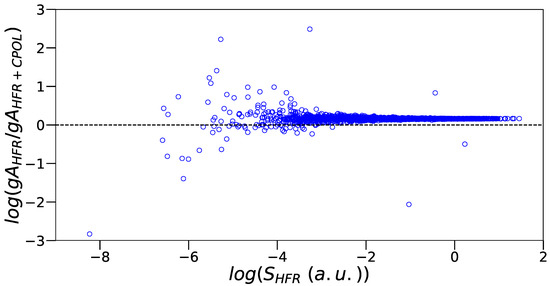
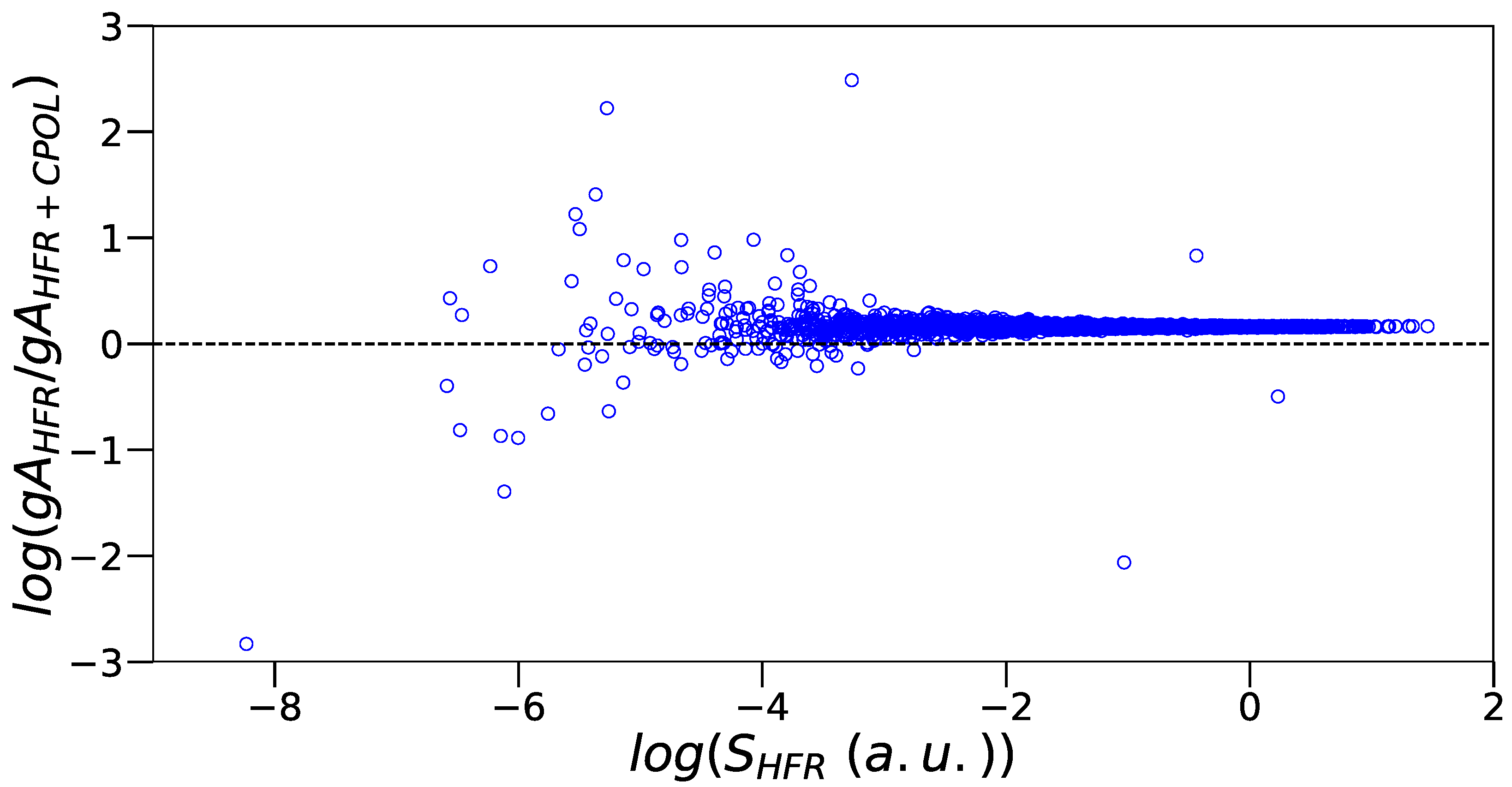
Figure 4 shows the logarithm of the ratio of the weighted transition probabilities determined by our HFR and HFR + CPOL models, namely $log(g{A}_{HFR}/g{A}_{HFR+CPOL})$, as a function of the logarithm of the HFR line strength, i.e., $log\left(S_{HFR}(a.u.)\right)$. This is the standard plot suggested by Kramida [17] where a less accurate data set, here HFR, is compared to a more accurate one, here HFR + CPOL, in order to evaluate its uncertainty. This is actually so because our HFR model neglects the core-polarization effects that systematically decrease the radiative decay rates and therefore systematically increase the level lifetimes. The importance of these effects has been demonstrated by comparing HFR + CPOL lifetimes with precise time-resolved laser-induced fluorescence measurements, notably in W III [6] (an ion belonging to the same isoelectronic sequence). From the figure, one can see that this is indeed the case; $g{A}_{HFR+CPOL}$ values are systematically shorter than those of HFR for the strongest lines ($S_{HFR}>10$ a.u.), and this is reflected in the average of the ratios (1.46). For these lines, there is also a statistical error affecting the HFR rates determined by the standard deviation of the corresponding rates (0.01). Both uncertainties (systematic and statistical) are taken into account in the uncertainty indicators $Un{c}_{HFR}$ reported in Table 3.

Figure 4. Comparison between the transition probabilities determined by our HFR model, $g{A}_{HFR}$, and those obtained by our HFR + CPOL calculation, $g{A}_{HFR+CPOL}$. Their ratios are plotted versus the corresponding HFR line strengths, $S_{HFR}$, both in the logarithmic scale. The straight line of equality is also shown. The uncertainties on our HFR rates as defined by the NIST [16] have been deduced from this plot following the procedure described by Kramida [17]. For the strongest transitions, namely $S_{HFR}>10$a.u., the average and the standard deviation of these ratios are 1.46 and 0.01 respectively.

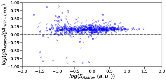
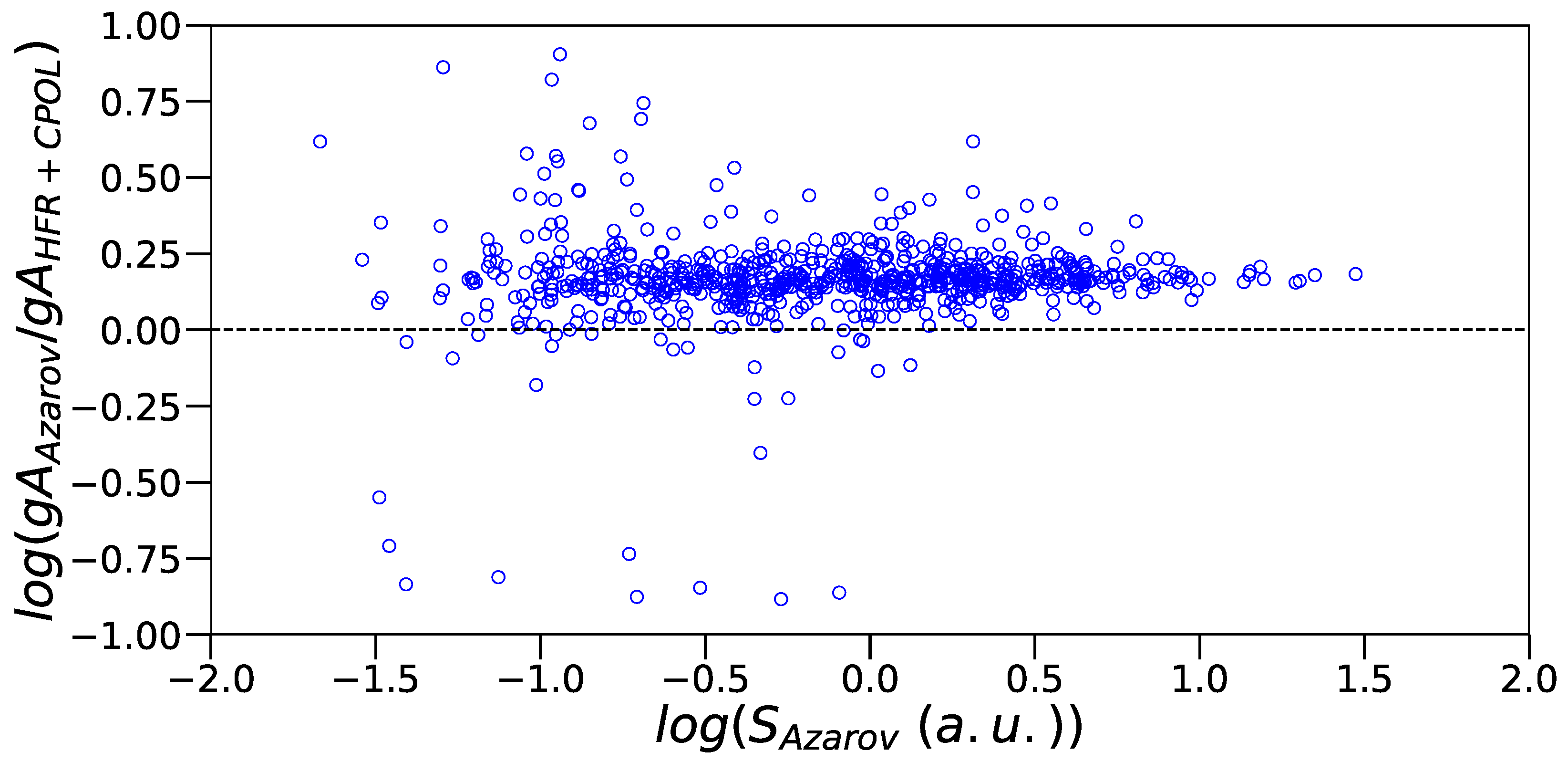
Concerning the transition probabilities computed by Azarov et al. [3] for 524 transitions, they are affected by a similar systematic uncertainty to our HFR model due to the neglect of core-polarization effects in their model, especially in their transition dipole integrals. Indeed, this is illustrated in Figure 5, used to evaluate their uncertainty indicators $Un{c}_{AZA}$ (see Table 3), where, for the strongest lines ($S_{Azarov}>10$ a.u.), the average of the ratios, $g{A}_{Azarov/g{A}_{HFR+CPOL}}$, is equal to 1.50, showing a systematic uncertainty of 50%, similar to HFR. The corresponding statistical uncertainty is 5%, as reflected in the standard deviation of the ratios (0.05).

Figure 5. Comparison between the transition probabilities determined by Azarov et al. [3], $g{A}_{Azarov}$, and those obtained by our HFR + CPOL calculation, $g{A}_{HFR+CPOL}$. Their ratios are plotted versus the corresponding line strengths, $S_{Azarov}$, deduced from Azarov et al. [3]. A-values are both in the logarithmic scale. The straight line of equality is also shown. The uncertainties in the rates of Azarov et al. [3] as defined by the NIST [16] have been deduced from this plot following the procedure described by Kramida [17]. For the strongest transitions, namely $S_{Azarov}>10$a.u., the average and the standard deviation of these ratios are 1.50 and 0.05 respectively.

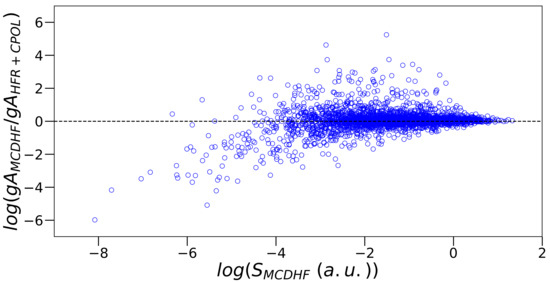
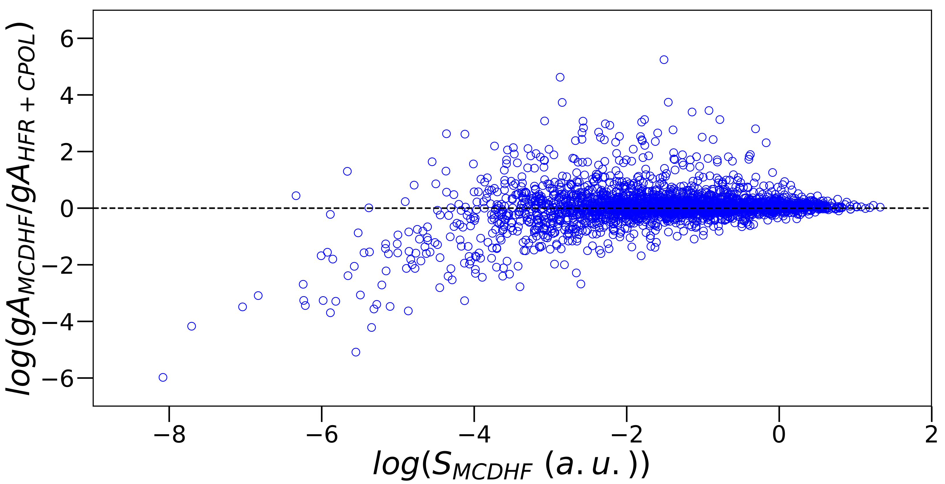
Regarding our MCDHF-RCI model, it includes part of the core–valence and core–core effects by explicitly promoting up to two electrons from the upper part of the core orbitals (4f, 5s and 5p) to correlation orbitals, and therefore it is expected that these will reduce the systematic uncertainty seen in the HFR and Azarov [3] models that both neglect core-polarization effects. In Figure 6, the same kind of plot as in Figure 4 and Figure 5 is presented for our MCDHF-RCI transition probabilities, $g{A}_{MCDHF}$, with respect to our HFR + CPOL values that are used as a reference. As a matter of fact, the average and the standard deviation of the ratios, $g{A}_{MCDHF}/g{A}_{HFR+CPOL}$, are 1.09 and 0.09 respectively, considering only the strongest transitions with $S_{MCDHF}>10$ a.u; thus their systematic uncertainty is reduced to 9%, which is included in the corresponding $Un{c}_{RCI}$ uncertainty indicators in Table 3.

Figure 6. Comparison between the transition probabilities determined by our MCDHF-RCI model, $g{A}_{MCDHF}$, and those obtained by our HFR + CPOL calculation, $g{A}_{HFR+CPOL}$. Their ratios are plotted versus the corresponding MCDHF-RCI line strengths, $S_{MCDHF}$, both in the logarithmic scale. The straight line of equality is also shown. The uncertainties in our MCDHF-RCI rates as defined by the NIST [16] have been deduced from this plot following the procedure described by Kramida [17]. For the strongest transitions, namely $S_{MCDHF}>10$a.u., the average and the standard deviation of these ratios are 1.09 and 0.09 respectively.

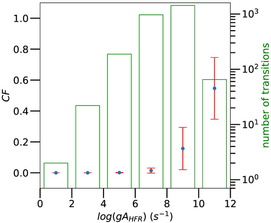
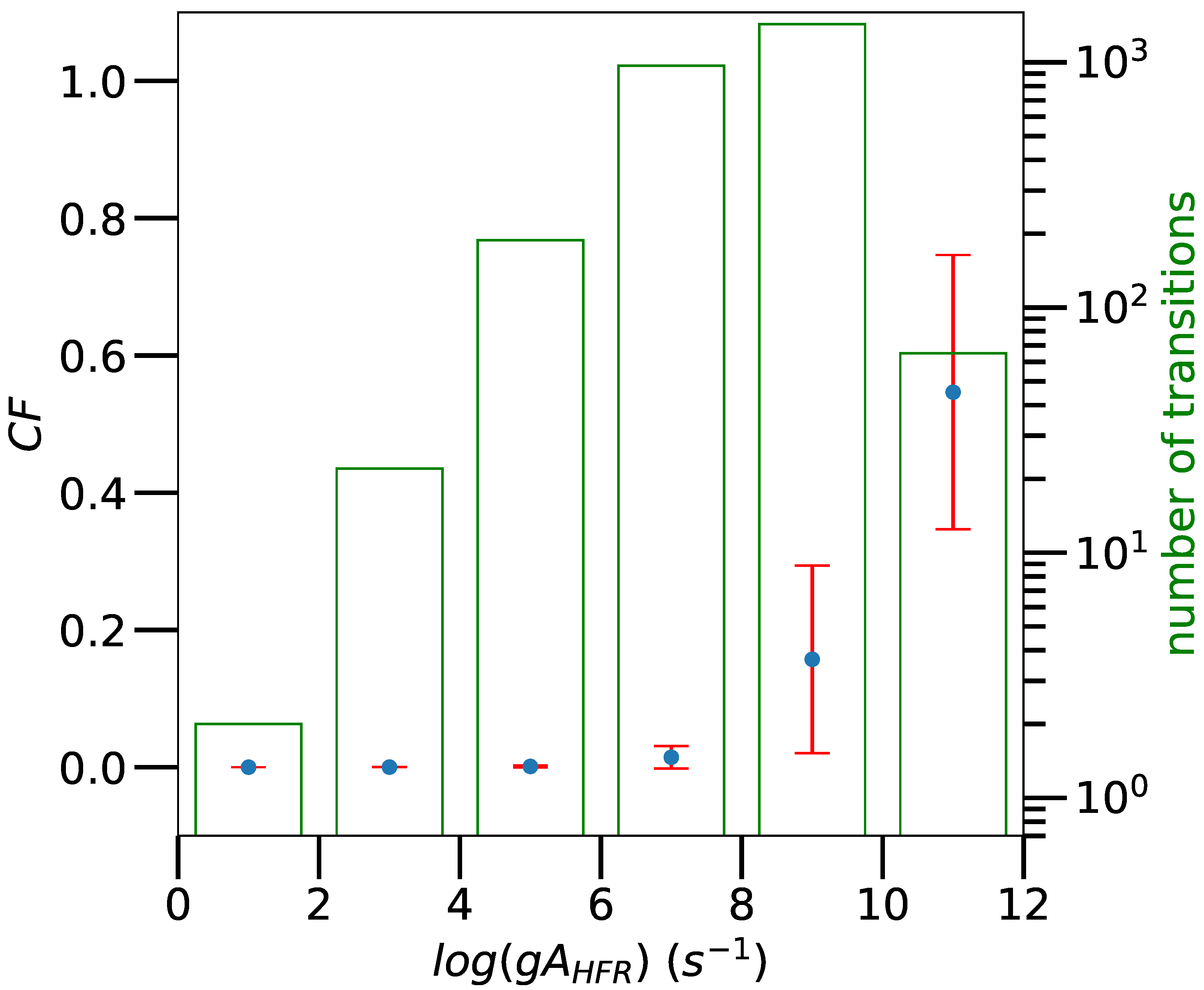
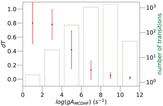
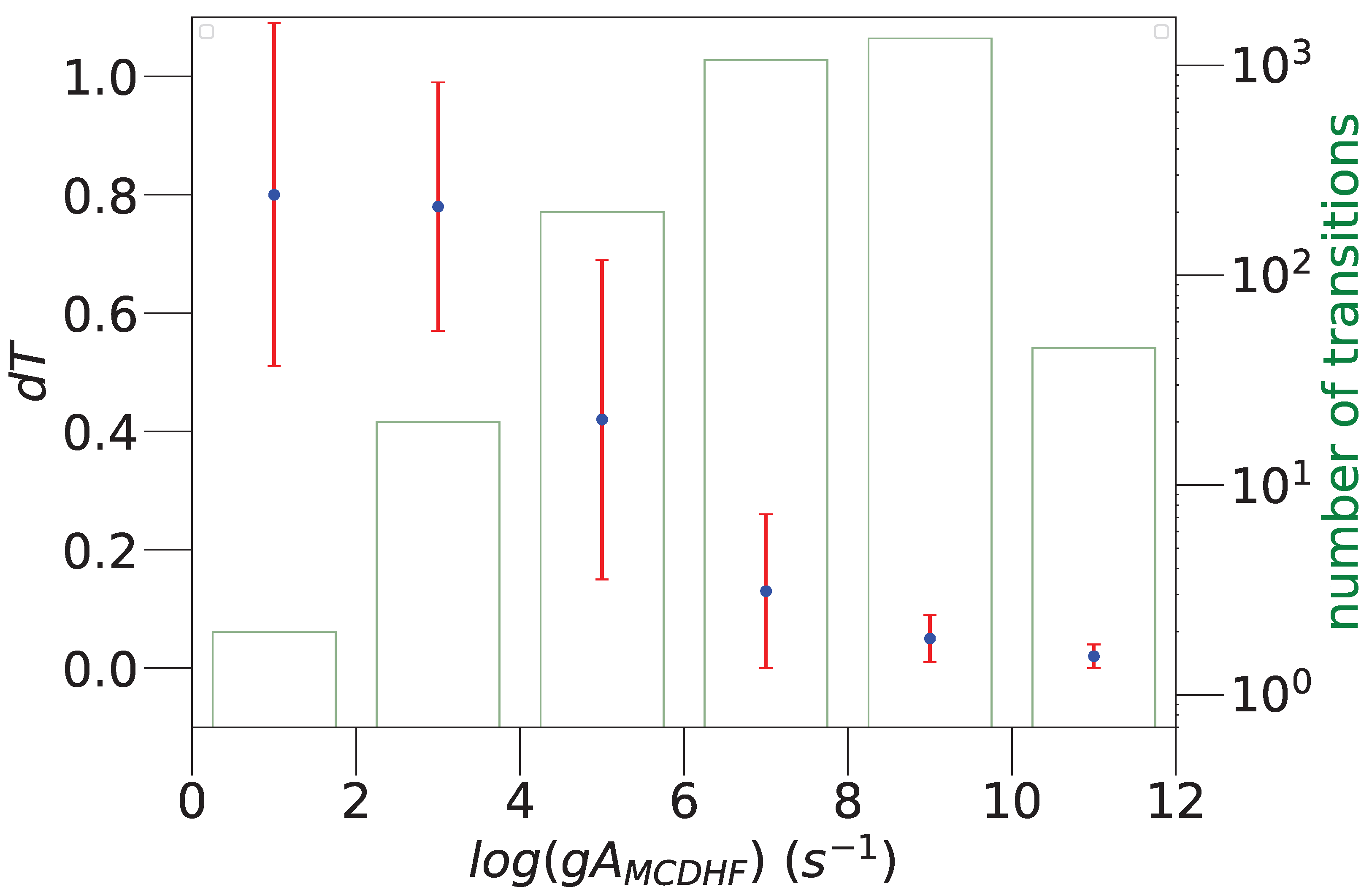
In addition, the cancellation factor $CF$ [4] for our HFR rates and the uncertainty indicator $dT$ [15] measuring the gauge agreement of our MCDHF-RCI rates are plotted versus their corresponding weighted transition probabilities in Figure 7 and Figure 8 respectively. Both figures show that most of the weak transitions (with $gA<{10}^8$ s⁻¹) are affected by either strong cancellation effects ($CF<0.05$) rendering their transition probabilities even weaker [4] or by poor gauge agreements ($dT>0.2$). These explain most of the dispersions seen for these weak lines in Figure 4, Figure 5 and Figure 6 as they are model-sensitive.

Figure 7. Cancellation factors [4], $CF$, as a function of our HFR weighted transition probability, $g{A}_{HFR}$, for Os V transitions. Each point is a mean value in each $gA$-value bin and the corresponding error bar represents the standard deviation. The numbers of transitions are also given in each bin as a histogram.

Figure 8. Uncertainty indicator [15], $dT$, as a function of our MCDHF-RCI weighted transition probability, $g{A}_{MCDHF}$, for Os V transitions. Each point is a mean value in each $gA$-value bin and the corresponding error bar represents the standard deviation. The numbers of transitions are also given in each bin as a histogram.

Finally, from Table 3, one can see that out of the 2677 HFR rates 856 have an uncertainty indicator $Un{c}_{HFR}$ ranked D (≤50%) and 1821 have a rank of E (>50%). Concerning our 2677 MCDHF transition probabilities, the corresponding statistics of the uncertainty indicator $Un{c}_{RCI}$ are one of rank A (≤3%) , one of rank B+ (≤7%), two of rank B (≤10%), five of rank C+ (≤18%), nine of rank D+ (≤40%), 15 of rank D (≤50%) and 2644 of rank E (>50%). Finally, all the $gA$-values computed by Azarov et al. [3] for 730 E1 transitions that classified their 703 observed lines have an uncertainty indicator $Un{c}_{AZA}$ ranked E (>50%).

4. Conclusions

The Einstein coefficients for the spontaneous emission process have been computed for the 2677 electric dipole transitions in Os V falling in the spectral range between 400 Å and 12,000 Å. The present study considerably extends the radiative data available compared to those previously determined by Azarov et al. [3] for 703 lines. A multiplatform approach as well as comparisons with the calculations published in Ref. [3] have been employed in order to evaluate the accuracy of the calculated transition probabilities, as no experimental values are available in the literature. The former consisted of building three independent models, two based on the HFR method [4], i.e., a HFR model that neglected the core-polarization effects and a HFR + CPOL model that included them and is equivalent to the HFR+CP(B) model used in W III [6] (where those effects were successfully tested through a comparison with TR-LIF measurements) and to the one built for Re IV [7] belonging to the same isoelectronic sequence, and one based on the MCDHF method [5,11] using the strategy adopted in Re IV [7]. The comparison between, on one side, our HFR $gA$-values and the ones computed by Azarov et al. [3] and, on the other side, our HFR + CPOL values showed a systematic discrepancy of ∼50% due to the lack of core-polarization effects in the former. Concerning our MCDHF transition probabilities, as their values take into account part of those effects, this systematic discrepancy is reduced to 9%. As these systematic errors will be added to the statistical ones, this justifies the choice of our HFR + CPOL rates to be used as a reference to evaluate the uncertainty indicators, $Unc$, [16] of the other three $gA$-value sets using the procedure described by Kramida [17]. They are determined for the first time in Os V. Therefore, we recommend our HFR + CPOL transition probabilities in expectation of an experimental benchmarking.

References

- Linsmeier, C.; Rieth, M.; Aktaa, J.; Chikada, T.; Hoffmann, A.; Houden, A.; Kurishita, H.; Jin, X.; Li, M.; Litnovsky, A.; et al. Development of advanced high heat flux and plasma-facing materials. Nucl. Fusion 2017, 57, 092007. [Google Scholar] [CrossRef] [Scilit]
- Gilbert, M.R.; Sublet, J.C. Neutron-induced transmutation effects in W and W-alloys in a fusion environment. Nucl. Fusion 2011, 51, 043005. [Google Scholar] [CrossRef] [Scilit]
- Azarov, V.I.; Raassen, A.J.J.; Joshi, Y.N.; Uylings, P.H.M.; Ryabtsev, A.N. Analysis of the Spectrum of the (5d4 + 5d36s) − 5d36p System of Four Times Ionized Osmium (Os V). Phys. Scr. 1997, 56, 325. [Google Scholar] [CrossRef] [Scilit]
- Cowan, R.D. The Theory of Atomic Structure and Spectra; University of California Press: Berkeley, CA, USA, 1981. [Google Scholar]
- Grant, I.P. Relativistic Quantum Theory of Atoms and Molecules. Theory and Computation; Springer: New York, NY, USA, 2007. [Google Scholar]
- Palmeri, P.; Quinet, P.; Fivet, V.; Biémont, E.; Nilsson, H.; Engström, L.; Lundberg, H. Lifetime measurements and calculated transition probabilities in W III. Phys. Scr. 2008, 78, 015304. [Google Scholar] [CrossRef] [Scilit]
- Brasseur, M.; Gamrath, S.; Quinet, P. Radiative decay rates for electric dipole transitions in doubly-, trebly- and quadruply-charged rhenium ions (Re III—V) of interest to nuclear fusion research and astrophysical spectra analyses. At. Data Nucl. Data Tables 2024, 157, 101636. [Google Scholar] [CrossRef] [Scilit]
- Quinet, P.; Palmeri, P.; Biémont, E.; McCurdy, M.M.; Rieger, G.; Pinnington, E.H.; Wickliffe, M.E.; Lawler, J.E. Experimental and Theoretical Radiative Lifetimes, Branching Fractions and Oscillator Strengths in Lu II. Mon. Not. R. Astron. Soc. 1999, 307, 934. [Google Scholar] [CrossRef] [Scilit]
- Quinet, P.; Palmeri, P.; Biémont, E.; Li, Z.S.; Svanberg, S. Radiative Lifetime Measurements and Transition probability Calculations in Lanthanide Ions. J. Alloys Compd. 2002, 344, 255. [Google Scholar] [CrossRef] [Scilit]
- Fraga, S.; Karwowski, J.; Saxena, K.M.S. Handbook of Atomic Data; Elsevier: Amsterdam, The Netherlands, 1976. [Google Scholar]
- Froese Fischer, C.; Gaigalas, G.; Jönsson, P.; Bieroń, J. GRASP2018-A Fortran 95 version of the General Relativistic Atomic Structure Package. Comput. Phys. Commun. 2019, 237, 184. [Google Scholar] [CrossRef] [Scilit]
- Li, Y.T.; Wang, K.; Si, R.; Godefroid, M.; Gaigalas, G.; Chen, C.Y.; Jönsson, P. Reducing the computational load—Atomic multiconfiguration calculations based on configuration state function generators. Comput. Phys. Commun. 2023, 283, 108562. [Google Scholar] [CrossRef] [Scilit]
- Si, R.; Li, Y.; Wang, K.; Chen, C.; Gaigalas, G.; Godefroid, M.; Jönsson, P. Graspg—An extension to Grasp2018 based on configuration state function generators. Comput. Phys. Commun. 2025, 312, 109604. [Google Scholar] [CrossRef] [Scilit]
- Gaigalas, G.; Froese Fischer, C.; Rynkun, P.; Jönsson, P. JJ2LSJ Transformation and Unique Labeling for Energy Levels. Atoms 2017, 5, 6. [Google Scholar] [CrossRef] [Scilit]
- Ekman, J.; Godefroid, M.; Hartman, H. Validation and implementation of uncertainty estimates of calculated transition rates. Atoms 2014, 2, 215. [Google Scholar] [CrossRef] [Scilit]
- Kramida, A.; Ralchenko, Y.; Reader, J.; NIST ASD Team. NIST Atomic Spectra Database (Ver. 5.12); National Institute of Standards and Technology: Gaithersburg, MD, USA, 2024. Available online: https://physics.nist.gov/asd (accessed on 13 February 2026). [CrossRef] [Scilit]
- Kramida, A. Critical Evaluation of Data on Atomic Energy Levels, Wavelengths, and Transition Probabilities. Fusion Sci. Technol. 2013, 63, 313. [Google Scholar] [CrossRef] [Scilit]
Disclaimer/Publisher’s Note: The statements, opinions and data contained in all publications are solely those of the individual author(s) and contributor(s) and not of MDPI and/or the editor(s). MDPI and/or the editor(s) disclaim responsibility for any injury to people or property resulting from any ideas, methods, instructions or products referred to in the content. |
© 2026 by the authors. Licensee MDPI, Basel, Switzerland. This article is an open access article distributed under the terms and conditions of the Creative Commons Attribution (CC BY) license.