


Abstract
We propose a method to measure the time delay of the Five-hundred-meter Aperture Spherical radio Telescope (FAST) using baseband data and periodic noise injection. By applying a sliding time window and calculating the average standard deviation ratio over 1000 noise cycles, high-precision measurement of the noise-induced time delay is achieved. The proposed method offers several advantages, including a short recording duration, high measurement accuracy, and strong immunity to electromagnetic interference. It enables effective monitoring of hardware state changes in the signal chain, and provides technical support for the future participation of the FAST in radio interferometry.
1. Introduction
The Five-hundred-meter Aperture Spherical radio Telescope (FAST), a major piece of national science and technology infrastructure completed during China’s 11th Five-Year Plan, is currently the most sensitive single-dish radio telescope in the world. Since routine operations began in January 2020, the FAST has delivered a series of ground-breaking results in frontier areas such as pulsars, fast radio bursts, neutral hydrogen, and gravitational waves (through pulsar timing array) [1,2,3,4,5,6,7], significantly advancing radio astronomy in China. Precise flux density calibration is essential to these achievements, and the noise diode mounted at the receiver front end serves as the primary calibration device.
During calibration, switching on the noise diode superimposes a known noise power spectrum onto the sky signal. Using the frequency-dependent noise-temperature relation determined in the laboratory, the standard “on-off” procedure converts the receiver output into an equivalent noise temperature, thereby establishing the flux density scale. For this conversion to be accurate, the exact timing of the noise injection must be known. In practice, however, radio-frequency signals travel from the reflector through the feed and amplifiers and are then transported by optical fibers to the digital backend.
The speed of light in fiber is only about 0.7 times that in a vacuum [8], so a 2 km fiber already introduces a delay of approximately 10 s.
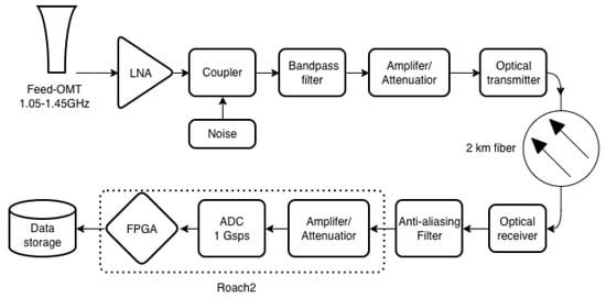
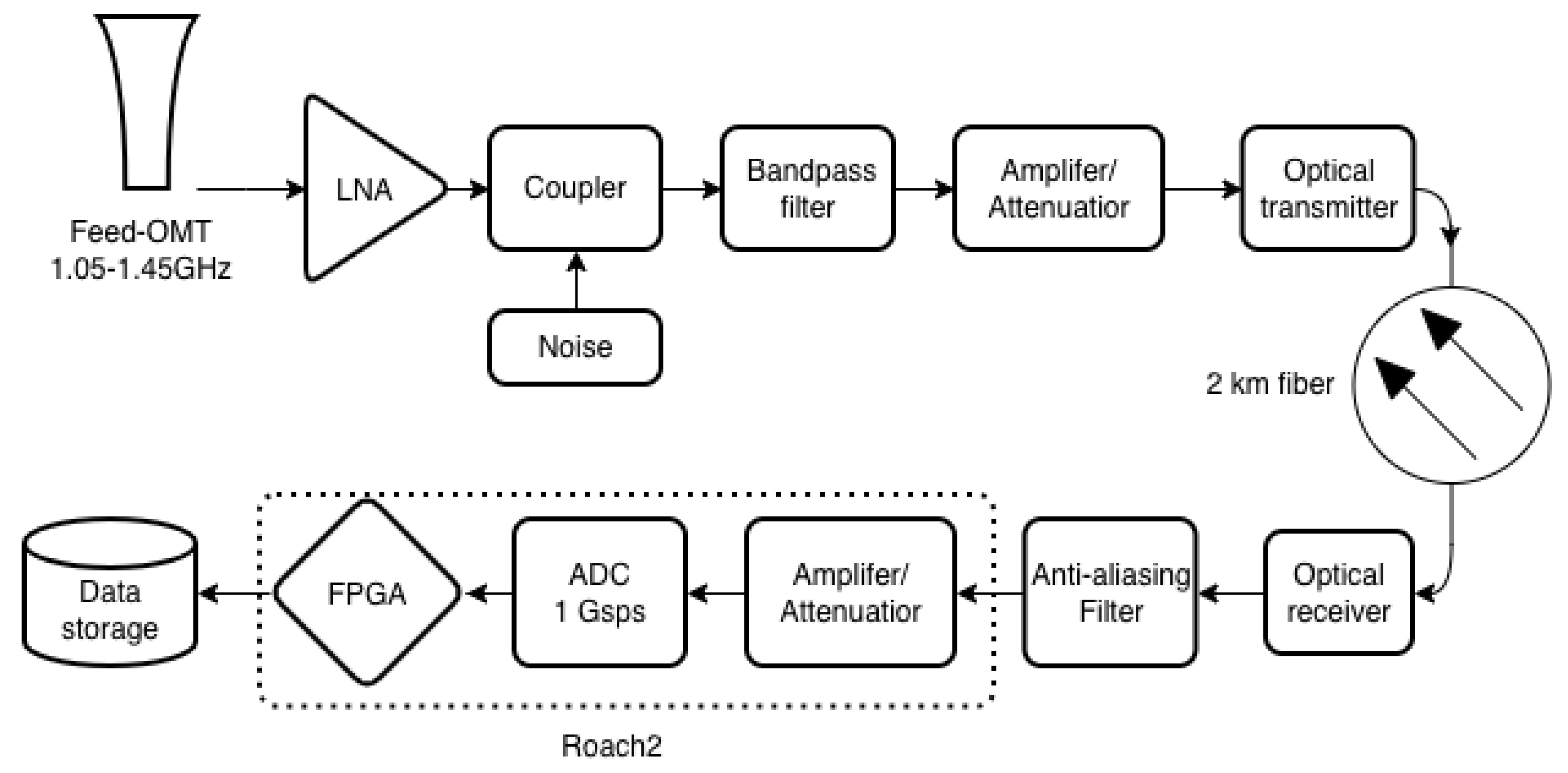
Figure 1 shows a simplified block diagram of the FAST 19-beam receiver signal chain. The signal chain consists of the feed-OMT (Ortho-Mode Transducer), low-noise amplifier (LNA), bandpass filter, amplifiers and attenuators, optical transmitter, 2 km optical fiber link, optical receiver, anti-aliasing filter, Analog-to-Digital Converter (ADC), and Field-Programmable Gate Array (FPGA) module. Since the 19-beam observation frequency (1.05–1.45 GHz) falls in the fourth Nyquist zone with a 1 GHz sampling rate, this signal chain does not employ conventional local oscillators or mixers. The data processed by the ROACH2 (Reconfigurable Open Architecture Computing Hardware, Digicom Electronics, Santa Clara, CA, USA) can be stored as either non-channelized power spectral data or baseband data.
Figure 1.
Simplified block diagram of the FAST 19-beam receiver signal chain. Arrows indicate the direction of signal flow through the chain.
In the FAST configuration, the calibration noise is coupled into the signal path downstream of the LNA through a directional coupler. The timing of the injected-noise switching and the ADC sampling is derived from the same hydrogen maser. The injected-noise source is switched between the ON and OFF states under the control of the 1 PPS signal, while the ROACH2 ADC sampling clock is referenced to the 10 MHz signal. However, both the noise-diode control command and the corresponding status feedback signal are transmitted over 2 km fibers, resulting in a total two-way propagation delay of approximately 20 s.
This delay is not negligible. In the FAST’s high-time-resolution pulsar observing mode, the sampling interval is about 49 s. A 20 s shift therefore amounts to 40% of the sampling period—large enough to systematically bias flux density calibration.
A common empirical approach to estimate this delay is to scan over a set of trial delay compensations and compute the on–off power ratio for each; the compensation that maximizes the ratio is taken as a coarse delay. This method exhibits three notable drawbacks. First, the measurement accuracy is limited to the microsecond level. Second, a single delay measurement takes about ten minutes, and a complete scan can require several hours, making the procedure feasible only during telescope maintenance periods. Third, it is susceptible to electromagnetic interference (EMI), because interference that fluctuates on timescales much shorter than the observation window can distort the power spectrum and further degrade accuracy.
An alternative technique employs loop-back fibers and a pulse-per-second (PPS) signal to calibrate the fiber delay [9,10]. The delay is obtained from the time difference between the transmitted and received PPS timestamps. However, this method isolates only the contribution of the optical fibers and cannot measure delays introduced by other components such as photoelectric conversion modules and coaxial cables.
Phase calibration (pcal) signals offer another possibility: injecting a comb-like spectrum can precisely correct the delay of the entire signal chain [11,12,13]. Nevertheless, this approach requires an additional narrow-pulse generation module at the receiver front end and dedicated software for signal extraction and processing, which limits its applicability to specific observing modes.
In contrast, baseband data—the raw, un-averaged voltage samples from the ADC—retain the full timing information at the sampling resolution. Because no time averaging is applied, the temporal precision of baseband data equals the sampling period of the ADC. Motivated by this advantage, we propose a method that combines baseband recordings with periodic noise injection to measure the transmission-path time delay with high precision. The method requires only short data captures, does not interfere with normal observations, and exhibits strong immunity to EMI.
2. Basic Principle
Our method builds on a simple property of zero-mean baseband noise: the average power is proportional to the voltage variance [14,15]:
where is the sample variance of the baseband voltage, R is the characteristic impedance (typically 50 ), k is the Boltzmann constant, B is the equivalent noise bandwidth, and T is the total system noise temperature. When the antenna points to the cold sky, , where is the antenna system temperature and is the injected noise temperature.
Equation (1) implies that the variance of the baseband voltage can directly reflect changes in noise power. If a periodic noise source is injected, the total power—and hence the variance—rises and falls in sync with the modulation. We exploit this to locate the exact moment the noise state changes.
The FAST currently uses a 19-beam receiver with a system temperature of approximately 20 K [16]. The noise diodes of this receiver can be set to 10 K or 1 K noise temperature. For the periodic noise injection experiment, the 10 K noise source is selected. When the noise diode is switched on, the total temperature is , and the corresponding sample variance is . When the noise diode is off, the total temperature is , and the variance is .
Consider a time window with a length equal to the injection period , and compute the ratio of the variances from the first and second halves of the window. When the window is perfectly aligned with the noise injection—i.e., the first half contains only signals with injected noise and the second half contains only signals without injected noise—the variance ratio is . Conversely, if the first half contains no injected noise and the second half contains injected noise, the ratio is . By sliding this time window, the variance ratio can be varied between the extreme values of 1.5 and 2/3. The sliding time offset at which the maximum is reached corresponds to the time delay of the noise diode.
Due to the finite response time of the noise diode, the variance ratio does not exhibit a sharp spike within the response period. Therefore, we aim to achieve a timing accuracy of approximately 100 ns, which is comparable to the typical response time of the noise diode.
3. Method Procedure
The specific implementation steps of this method include five key components:
3.1. Selection and Injection of Periodic Noise
The variance ratio ranges between and . Choosing the stronger 10 K noise yields a range of , whereas the weaker 1 K noise gives . To clearly observe the variation in the ratio, the 10 K noise injection is preferred.
Furthermore, an appropriate noise injection period must be chosen. When computing the average standard deviation ratio (for computational convenience, the standard deviation is used instead of the variance), data from multiple periods are averaged. If the period is too large, the total measurement and data processing time increases; if too small, the calculated time delay may need to be corrected by integer multiples of the period. Considering that the round-trip fiber length is about 4 km, contributing roughly 20 s of delay, and the delay from other devices is typically less than 10 s, a noise period of 30–50 s is appropriate.
To determine the noise diode state, the first two cycles are set to the “off” state.
3.2. Acquisition and Preprocessing of Baseband Voltage Signals
Using the existing ROACH2 digital backend of the FAST [17], voltage signals are continuously recorded. ROACH2 employs eight-bit sampling, and the two polarization channels are interleaved. The signals of the same polarization must be extracted. The total recording length is generally set to 1000 noise cycles.
The standard deviation is calculated for every 200 samples, and the distribution over the first 10 cycles is plotted. The clear periodic fluctuation of the standard deviation confirms that the noise diode is correctly activated.
3.3. Calculation of the Average Standard Deviation Ratio
After discarding the first two cycles, the standard deviation of the first half and the second half of each cycle is computed, and their ratio is taken for each cycle. The average standard deviation ratio is then obtained by averaging the ratios over 1000 cycles. The time window is slid with a step size of four samples until the total sliding time reaches one full noise cycle. For each sliding step, the average ratio over 1000 cycles is calculated.
3.4. Analysis and Delay Extraction from the Ratio Curve
The average standard deviation ratio is plotted as a function of the sliding time offset. The extreme value of this curve determines the corresponding sliding time. Since the FAST’s noise injection sequence is “on” followed by “off”, the sliding time corresponding to the maximum value represents the noise time delay.
3.5. Recording and Analysis of Multi-Beam Delay Results
For the 19-beam receiver of the FAST, the noise time delay of each beam is measured. By comparing the delays obtained on different dates, the long-term variation in the noise time delay for each beam can be monitored.
4. Measurement Experiment
On 11 February 2026, during a routine source change in FAST observations, 1 s of baseband data from the 19-beam receiver was recorded using the ROACH2 digital backend. The 10 K high-level noise was selected, with a noise period of 50 s, and the noise diode was set to the off state for the first 100 s.
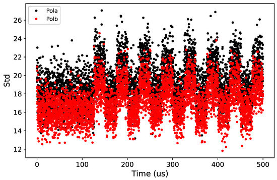
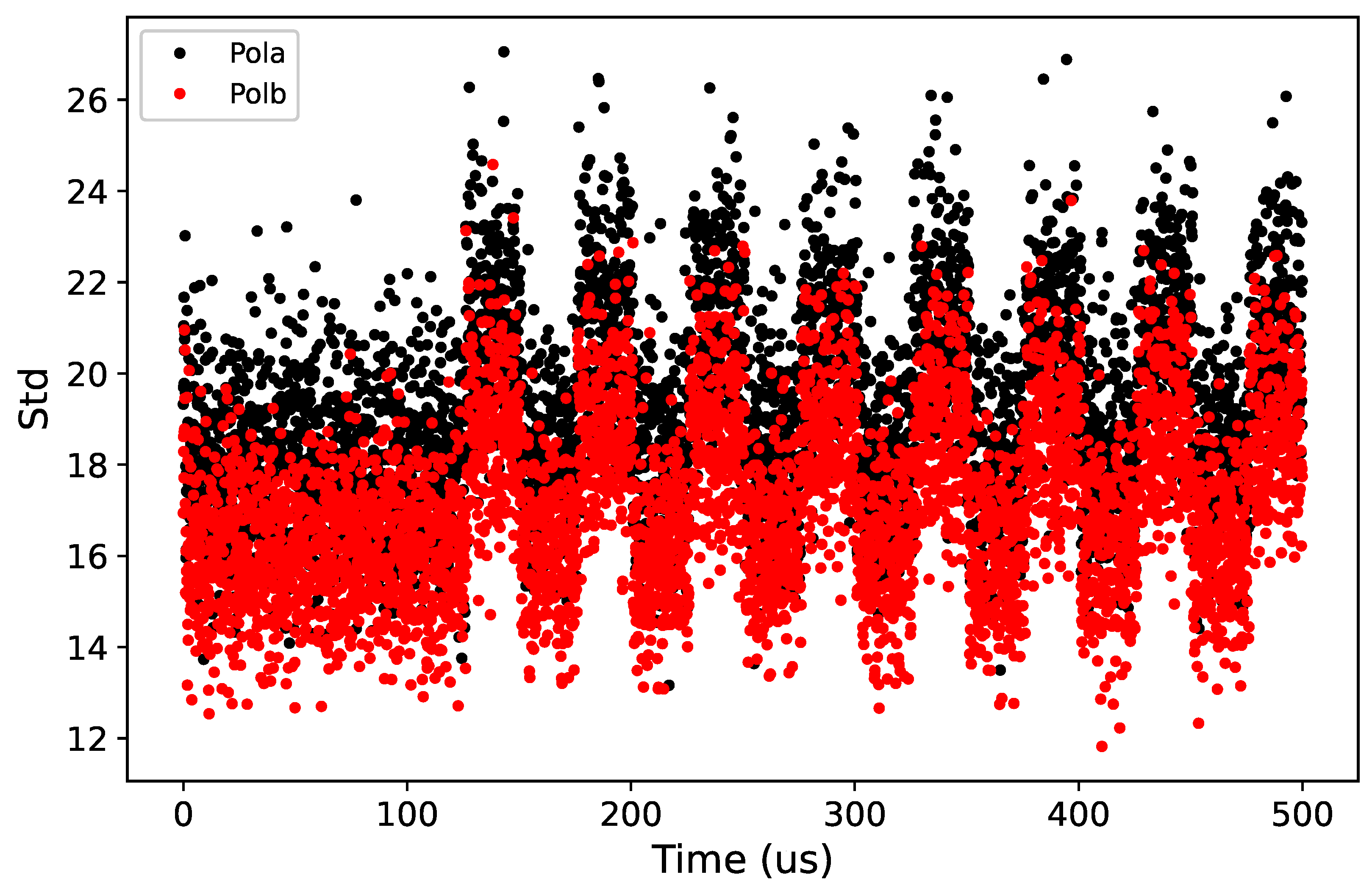
First, the standard deviation distribution for the first 10 cycles (500 s) was plotted (Figure 2). It can be seen that after about 120 s, the standard deviation exhibits periodic variations, confirming the activation of the noise diode.
Figure 2.
Standard deviation of beam M01 during the first 500 s. Red and black colors represent different polarizations.
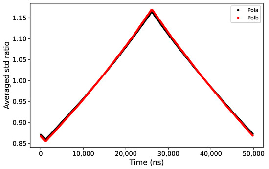
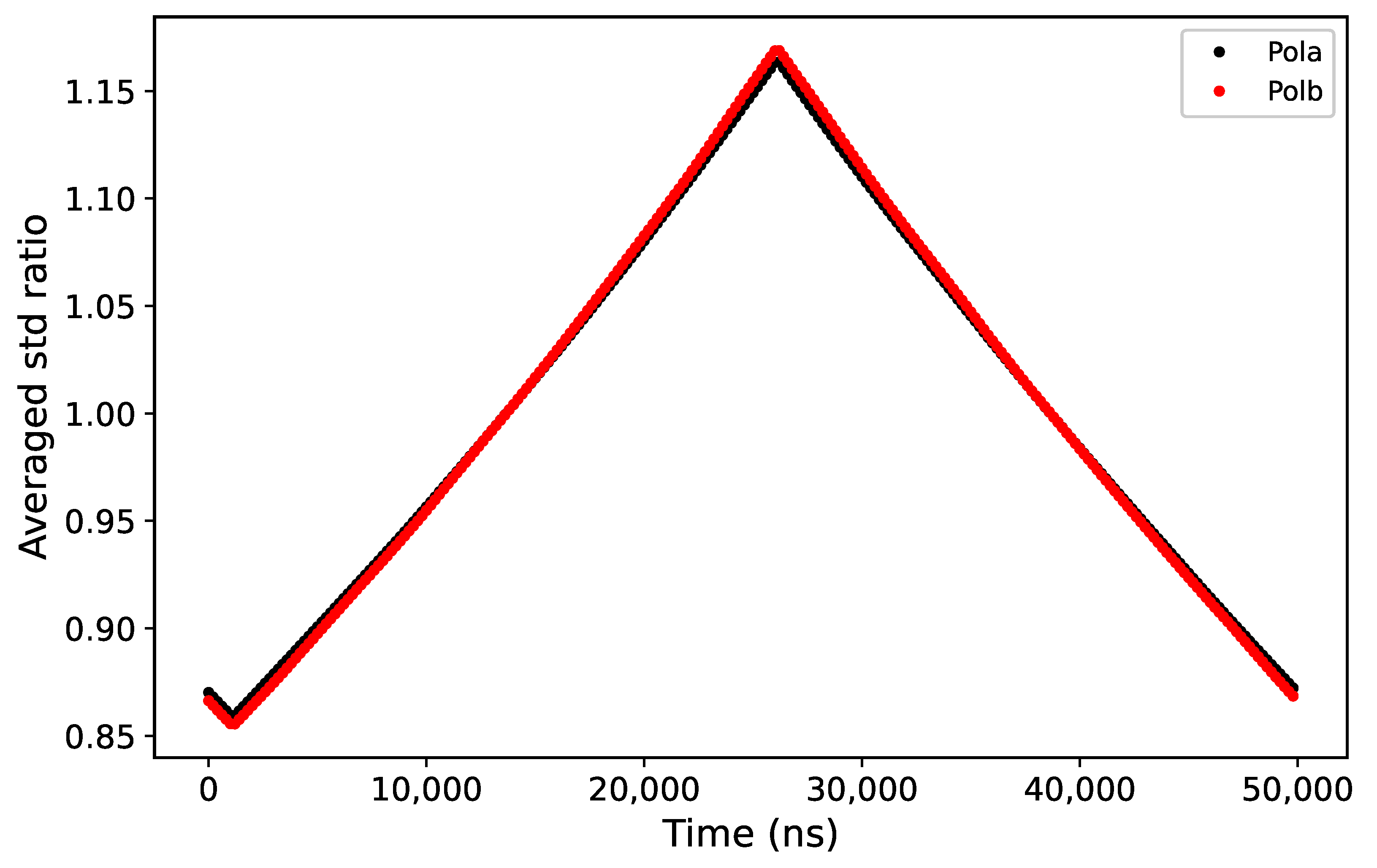
Using a sliding step of 200 ns, the average standard deviation ratio over 1000 cycles was plotted against the sliding time (Figure 3). The range of the maximum was determined, showing that the noise delay for beam M01 is approximately 26 s, while the minimum appears around 1 s.
Figure 3.
Average standard deviation ratio vs. sliding time with a step of 200 ns over 0–50 s. Red and black represent different polarizations.
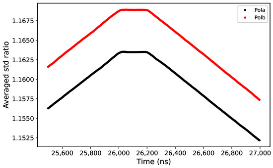
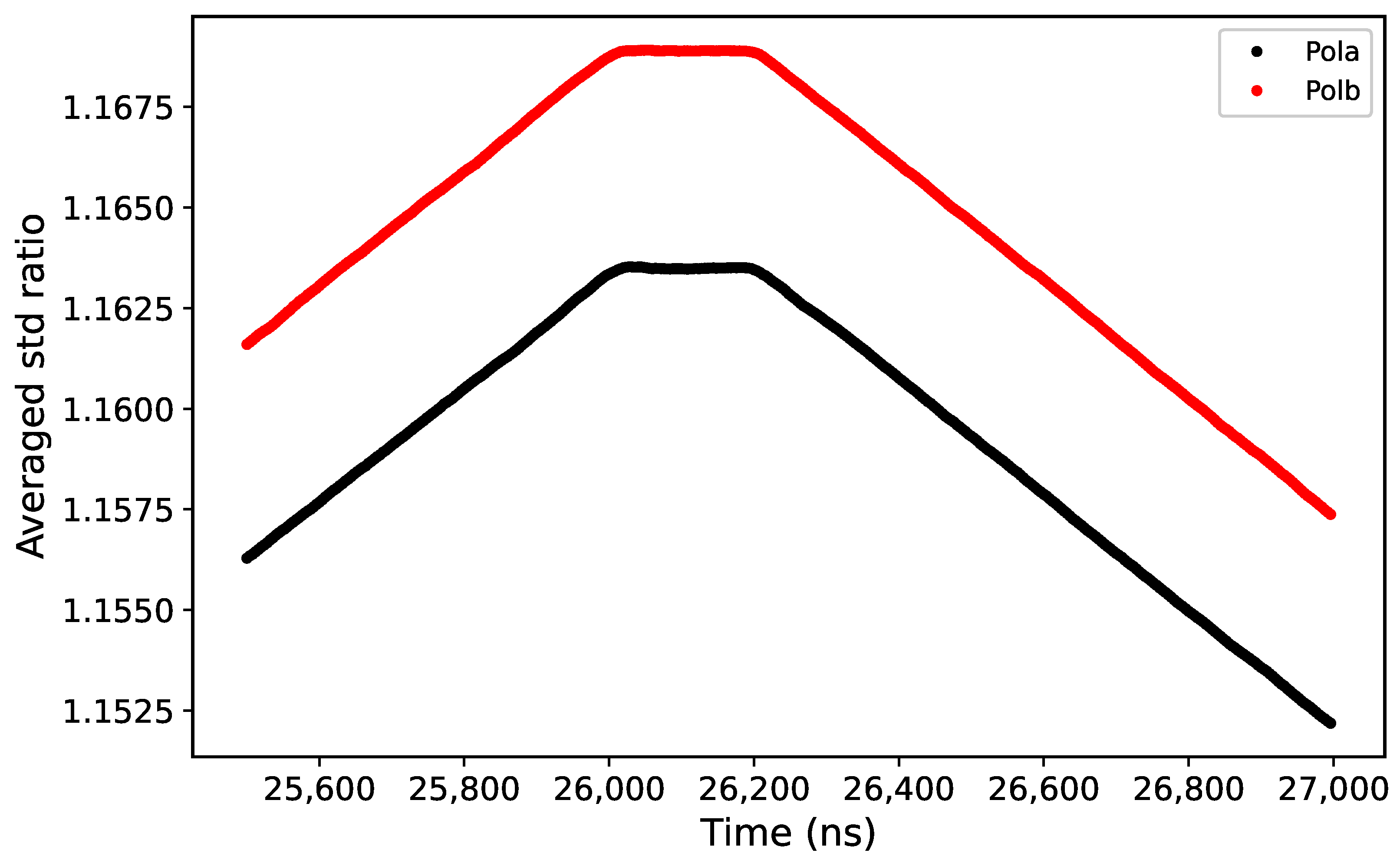
To precisely determine the maximum, the sliding step was reduced to 4 ns, and the sliding time range was restricted to 25.5–27 s. The resulting curve is shown in Figure 4.
Figure 4.
Average standard deviation ratio vs. sliding time with a step of 4 ns over 25.5–27 s. Red and black represent different polarizations.
In Figure 4, the average standard deviation ratio first increases linearly, reaches a plateau near 26 s, and begins to decrease around 26.2 s. A first-order polynomial was fitted to the straight lines on both sides of the plateau, and the intersection point of the two fitted lines yields the noise time delay for beam M01: 26.112 s for polarization A and 26.108 s for polarization B. Similarly, a first-order polynomial was fitted to the central plateau, and its intersection with the side fits defines the plateau’s time range (Figure 4): 26.010–26.214 s for polarization A and 26.008–26.208 s for polarization B.
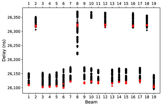
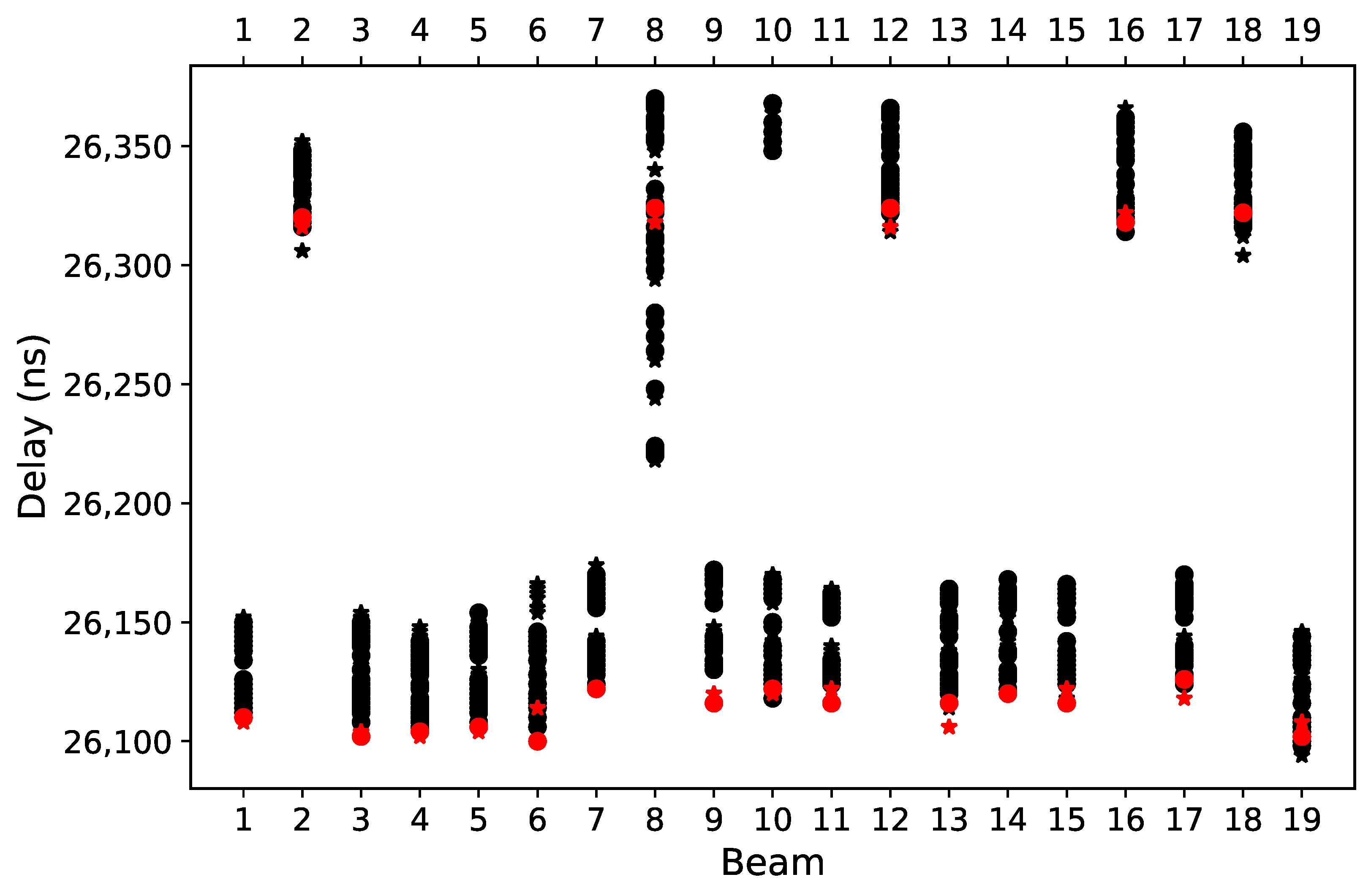
The same procedure was applied to all 19 beams. Figure 5 compares the noise time delays measured in this experiment (red) with historical results (black).
Figure 5.
Comparison of noise time delays for different beams. Circles and stars represent different polarizations; red indicates the current measurement.
All data processing and analysis were performed using Python (version 3.12.4, Python Software Foundation, Wilmington, DE, USA), along with the following key libraries: NumPy (v2.1.2) and Matplotlib (v3.9.2).
5. Results, Analysis and Discussion
In Figure 3, the extreme values of the average standard deviation ratio are 0.855 and 1.169, corresponding to a noise temperature of 10 K and an average system temperature of about 27 K, which is slightly higher than the nominal 20 K of the 19-beam receiver. This is because the average system temperature here includes electromagnetic interference from satellites.
In Figure 4, the extreme values for the two polarizations of beam M01 are 1.163 and 1.169. The small difference is attributed to a level difference in the analog signals.
The smoothness of the average standard deviation ratio curve in Figure 4 indicates that EMI had minimal impact on the results during these 1000 cycles.
The plateau observed in Figure 4 is primarily caused by the response time of the noise diode. The plateau duration encompasses twice the diode response time, which is estimated to be approximately 100 ns for the 19-beam receiver. The well-defined plateau also demonstrates that the target timing accuracy of 100 ns is fully satisfied by the experiment.
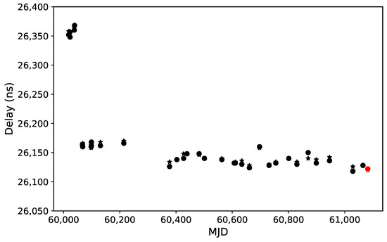
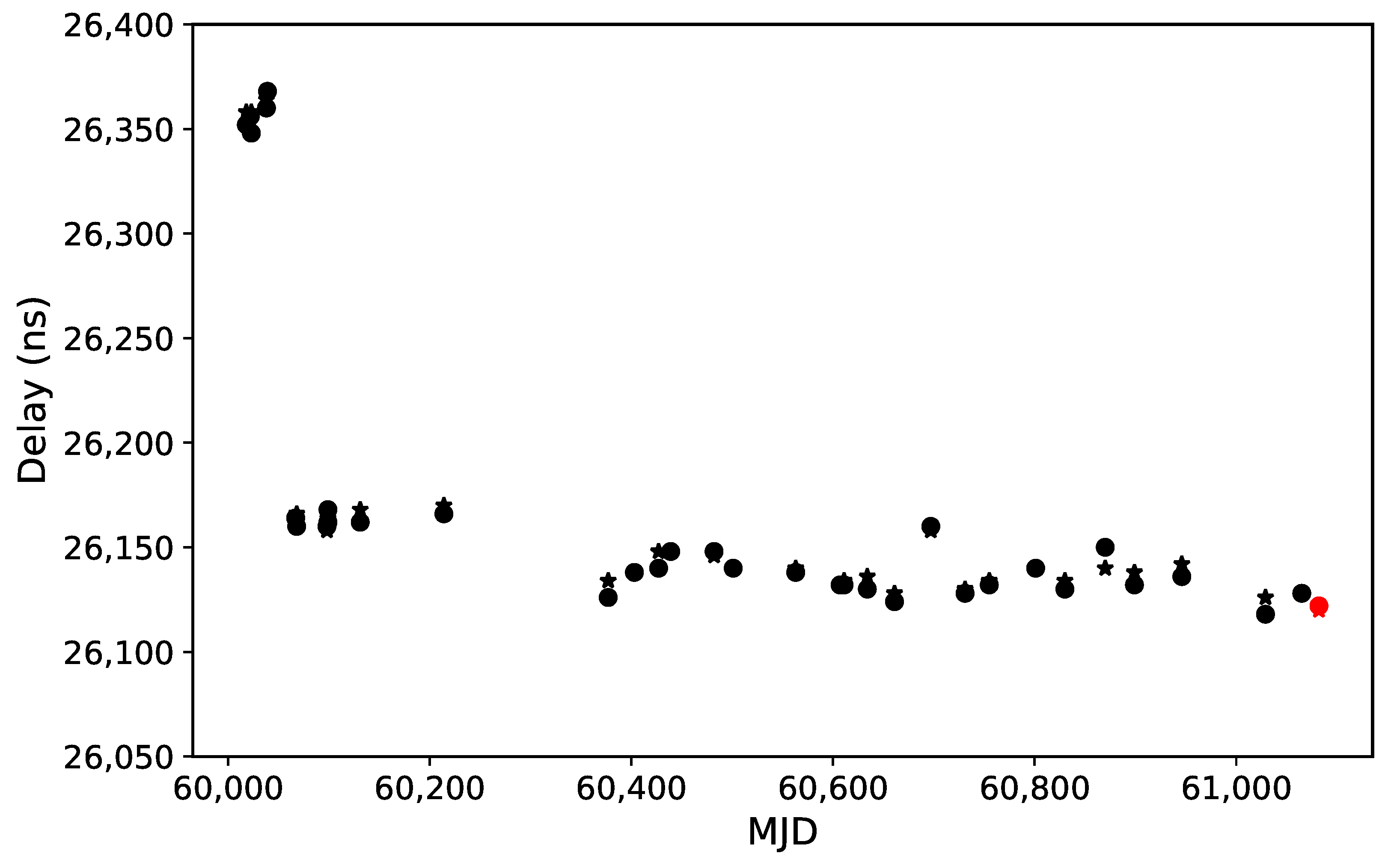
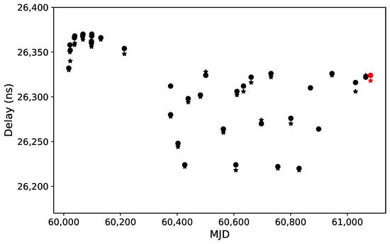
In Figure 5, the noise time delays of different beams cluster around 26.1 s or 26.3 s, due to inherent delay differences among devices of the same model [14]. In April 2023 (near MJD 60045), some components of the same model in beam 10 were replaced. As a result, its measured noise time delay jumped from about 26.3 s to about 26.1 s (Figure 6).
Figure 6.
Noise time delay distribution for beam 10 on different dates. Circles and stars represent different polarizations; red indicates the current measurement, while black represents historical records.
Furthermore, due to a reduction in fiber length in March 2024 (near MJD 60370), the noise time delays of most beams decreased by about 20 ns. Under stable fiber length conditions, the noise time delay generally fluctuates within a range of about 20 ns (Figure 6).
However, beam 8 exhibits a significantly larger fluctuation range (Figure 5). Under unchanged fiber conditions, its noise time delay fluctuates within about 100 ns (Figure 7), suggesting that the components in the signal chain of beam 8 have poorer stability compared to other beams.
Figure 7.
Noise time delay distribution for beam 8 on different dates. Circles and stars represent different polarizations; red indicates the current measurement, while black represents historical records.
6. Conclusions
This paper presents a method for measuring the time delay of the FAST using baseband data and periodic noise injection. The method exploits the proportional relationship between power and voltage variance, where the periodic noise drives variance fluctuations. By combining a sliding time window with the average standard deviation ratio over many cycles, high-precision time delay measurement is achieved. The method requires only a short data recording time, does not interfere with normal observations, produces a smooth average ratio curve over multiple cycles, and exhibits strong immunity to electromagnetic interference. By comparing the evolution of noise time delays, changes in components along the signal chain can be effectively monitored.
Author Contributions
Conceptualization, Y.Z.; methodology, R.-R.C. and Y.Z.; investigation, R.-R.C.; data curation, R.-R.C.; writing—original draft preparation, R.-R.C.; writing—review and editing, Y.Z.; visualization, R.-R.C.; supervision, H.-Y.Z.; project administration, H.-Y.Z. All authors have read and agreed to the published version of the manuscript.
Funding
This research was funded by the National Key Research and Development Program of China, grant numbers 2024YFA1611502, 2024YFA1611504, and 2022YFA1602904.
Data Availability Statement
The baseband data presented in this study are classified as engineering data under the FAST Data Policy and are therefore not open to the public.
Acknowledgments
This work made use of the data from FAST (Five-hundred-meter Aperture Spherical radio Telescope). FAST is a Chinese national mega-science facility, operated by National Astronomical Observatories, Chinese Academy of Sciences. The authors would like to express their gratitude to the FAST operational team for their technical support.
Conflicts of Interest
The authors declare no conflicts of interest. The funders had no role in the design of the study; in the collection, analyses, or interpretation of data; in the writing of the manuscript; or in the decision to publish the results.
References
- Nan, R.D. Five hundred meter aperture spherical radio telescope (FAST). Sci. China Ser. G Phys. Mech. Astron. 2006, 49, 129–148. [Google Scholar] [CrossRef] [Scilit]
- Ching, T.C.; Li, D.; Heiles, C.; Li, Z.-Y.; Qian, L.; Yue, Y.L.; Tang, J.; Jiao, S.H. An early transition to magnetic supercriticality in star formation. Nature 2022, 601, 49–52. [Google Scholar] [CrossRef] [Scilit] [PubMed]
- Han, J.L.; Wang, C.; Wang, P.F.; Wang, T.; Zhou, D.J.; Sun, J.-H.; Yan, Y.; Su, W.-Q.; Jing, W.-C.; Chen, X.; et al. The FAST galactic plane pulsar snapshot survey: I. Project design and pulsar discoveries. Res. Astron. Astrophys. 2021, 21, 107. [Google Scholar] [CrossRef] [Scilit]
- Feng, Y.; Li, D.; Yang, Y.P.; Zhang, Y.; Zhu, W.; Zhang, B.; Lu, W.; Wang, P.; Dai, S.; Lynch, R.S.; et al. Frequency-dependent polarization of repeating fast radio bursts—Implications for their origin. Science 2022, 375, 1266–1270. [Google Scholar] [CrossRef] [Scilit] [PubMed]
- Niu, C.H.; Aggarwal, K.; Li, D.; Zhang, X.; Chatterjee, S.; Tsai, C.-W.; Yu, W.; Law, C.J.; Burke-Spolaor, S.; Cordes, J.M.; et al. A repeating fast radio burst associated with a persistent radio source. Nature 2022, 606, 873–877. [Google Scholar] [CrossRef] [Scilit] [PubMed]
- Xu, C.K.; Cheng, C.; Appleton, P.N.; Duc, P.-A.; Gao, Y.; Tang, N.-Y.; Yun, M.; Dai, Y.S.; Huang, J.-S.; Lisenfeld, U.; et al. A 0.6 Mpc H I structure associated with Stephan’s Quintet. Nature 2022, 610, 461–466. [Google Scholar] [CrossRef] [Scilit] [PubMed]
- Pan, Z.C.; Lu, J.G.; Jiang, P.; Han, J.L.; Chen, H.-L.; Han, Z.W.; Liu, K.; Qian, L.; Xu, R.X.; Zhang, B.; et al. A binary pulsar in a 53-minute orbit. Nature 2023, 620, 961–964. [Google Scholar] [CrossRef] [Scilit] [PubMed]
- Saleh, B.E.A.; Teich, M.C. Fundamentals of Photonics, 3rd ed.; Wiley: Hoboken, NJ, USA, 2019. [Google Scholar]
- Siccardi, M.; Rovera, D.; Romisch, S. Delay measurements of PPS signals in timing systems. In Proceedings of the 2016 IEEE International Frequency Control Symposium (IFCS), New Orleans, LA, USA, 9–12 May 2016; pp. 1–6. [Google Scholar]
- Rost, M.; Fujieda, M.; Piester, D. Time transfer through optical fibers (TTTOF): Progress on calibrated clock comparisons. In Proceedings of the 24th European Frequency and Time Forum, Noordwijk, The Netherlands, 13–16 April 2010; pp. 1–8. [Google Scholar]
- Jacobs, C.S. Phase Calibration Tone Processing with the Block II VLBI Correlator; TMO Progress Report 42-134; NASA Jet Propulsion Laboratory: Pasadena, CA, USA, 1998. [Google Scholar]
- Chang, J.; Wang, J.Q.; Jiang, Y.C.; Shu, F.C. Method and application of measuring absolute link delay by pcal. Astron. Tech. Instrum. 2022, 19, 297–304. (In Chinese) [Google Scholar]
- Yang, Y.; Zheng, W.M. Software realization method of extracting VLBI phase calibration signal. Ann. Shanghai Obs. Acad. Sin. 2006, 27, 107–117. (In Chinese) [Google Scholar]
- Nyquist, H. Thermal agitation of electric charge in conductors. Phys. Rev. 1928, 32, 110–113. [Google Scholar] [CrossRef] [Scilit]
- Thompson, A.R.; Moran, J.M.; Swenson, G.W., Jr. Interferometry and Synthesis in Radio Astronomy, 3rd ed.; Wiley: Hoboken, NJ, USA, 2017. [Google Scholar]
- Jiang, P.; Tang, N.-Y.; Hou, L.-G.; Liu, M.-T.; Krčo, M.; Qian, L.; Sun, J.-H.; Ching, T.-C.; Liu, B.; Duan, Y.; et al. The fundamental performance of FAST with 19-beam receiver at L band. Res. Astron. Astrophys. 2020, 20, 64. [Google Scholar] [CrossRef] [Scilit]
- Li, J.Y.; Zhu, R.; Guo, S.; Rui, P.; Xu, Z. Development and performance validation of a versatile VLBI digital backend using ROACH2 platform. Publ. Astron. Soc. Pac. 2025, 137, 035001. [Google Scholar] [CrossRef] [Scilit]
Disclaimer/Publisher’s Note: The statements, opinions and data contained in all publications are solely those of the individual author(s) and contributor(s) and not of MDPI and/or the editor(s). MDPI and/or the editor(s) disclaim responsibility for any injury to people or property resulting from any ideas, methods, instructions or products referred to in the content. |
© 2026 by the authors. Licensee MDPI, Basel, Switzerland. This article is an open access article distributed under the terms and conditions of the Creative Commons Attribution (CC BY) license.