


Abstract
In this article, we derive the components of the entropy covector field for a relativistic kinetic gas composed of collisionless, spinless, massive, and uncharged particles following bound orbits in a curved spacetime background. By assuming a dependence on the inclination angle of the particle orbits, we consider two distinct models that describe a rotating and a non-rotating relativistic kinetic gas around a Schwarzschild black hole. We analyze the behavior of key macroscopic observables (including the anisotropy parameter and the kinetic temperature) which are constructed from the particle density, energy density, and principal pressures. We aim to characterize and compare the morphology of the resulting configurations, thereby extending and complementing a previous work. The results reveal significant differences between the rotating and non-rotating cases, particularly in the asymptotic behavior of the anisotropy parameter, kinetic temperature, and average pressure, highlighting the role of angular momentum in shaping the macroscopic properties of collisionless gases in strong gravitational fields.
1. Introduction
Kinetic theory is based on the principles of statistical mechanics and explains the macroscopic properties of the gas (such as pressure, temperature, entropy, particle density, etc.) from microscopic laws of physics. This theory can be treated through one of the key concepts, namely, the characterization of the state of the gas through the one-particle distribution function (DF) [1]. The DF is a time-dependent function defined on the one-particle phase space of the theory, whose time evolution is determined by Boltzmann’s equation [2,3,4]. The DF represents the averaged number of particles contained inside the volume element as at the nonrelativistic level.
Recent event horizon-scale images of and obtained by the Event Horizon Telescope Collaboration have established the presence of hot plasma in the immediate vicinity of supermassive black holes [5,6,7,8]. While the observed dynamics involve several physical ingredients, including magnetic fields, radiative processes, and plasma interactions, the gravitational field remains the fundamental mechanism governing particle motion. Motivated by these observations, it is natural to investigate simplified kinetic models in which particles move under the sole influence of gravity. Such models are particularly relevant in regimes where the mean free path is much larger than the characteristic size of the system, so that collision effects can be neglected and the matter content can be described as a collisionless Vlasov gas [9]. Although this approximation does not capture all the complexity of the plasma observed by the EHT, it provides a useful first step in understanding the kinetic structure of matter distributions around black holes and establishes a framework upon which additional physical effects can be incorporated.
This article studies the behavior of a relativistic kinetic gas in a strong gravitational field. In particular, we consider kinetic gas clouds orbiting black holes, and we explore different scenarios describing such configurations. We consider the case in which collisions between the gas particles, as well as effects of the self-gravity of the gas and the electromagnetic field, can be neglected as a starting point. This leads to the problem of solving the relativistic collisionless Boltzmann equation for the one-particle distribution function on a fixed spacetime background. Restricting ourselves to a spherically symmetric Schwarzschild black hole and choosing a DF depending solely on integrals of motion, the collisionless Boltzmann equation is solved automatically. From this one-particle DF of a simple gas, one can construct physical observables, through momentum averaging, that contain information about the particle, energy, and entropy densities; mean particle four-velocity; heat flow; pressure tensor; and the kinetic temperature. Our aim is to obtain an analytic understanding of what happens in these kinetic gas configurations for bounded trajectories. Since almost all the work on this problem deals with accretion rate and other phenomena, here we explore and complete this study of entropy and some other macroscopic observables for gas trajectories that are always trapped by this effective potential of the black hole. Furthermore, it is a starting point for generalizing bounded trajectories to more complex curved backgrounds and integrating other effects such as self-gravity of the gas, electromagnetic effects, etc.
For the development of this research, we assume a particular ansatz for the one-particle DF that describes a collisionless kinetic gas around a non-rotating black hole, motivated by the inclination angle of the particle’s orbits [10,11,12] and the generalized polytropic ansatz [13,14]. The dependence on the inclination angle allows us to consider two configurations of a relativistic kinetic gas: one with total angular momentum (rotating model) and another with zero angular momentum (non-rotating model). Since we are working with a collisionless gas, it is not possible to establish thermal equilibrium in any sense. Consequently, the DF, which is a solution of the Liouville vector field, can be written as a function that depends solely on the system’s constants of motion. In recent years, kinetic solutions have been developed for the stationary accretion of collisionless relativistic gases in Kerr [15,16] and Kerr–Newman [17] geometries. These studies focus on particles arriving from infinity and being captured by the black hole, so the relevant dynamics are dominated by unbounded trajectories characterized by specific energies above the maximum of the effective potential. From distribution functions defined by motional constants, particle currents, energy-momentum tensors, and accretion rates of mass, energy, and angular momentum have been calculated. The results indicate that the black hole spin introduces appreciable corrections to the absorption dynamics, while the electric charge produces a further decrease in accretion rates. Unlike the scenarios considered in [15,16,17], where the physics is dominated by particles following unbounded trajectories and being captured from infinity, in this work we focus on developing bounded trajectory configurations for entropy and some associated macroscopic observables, such as kinetic temperature and anisotropy in the principal pressures.
The main purpose of this article is to study and characterize the morphology of a collisionless relativistic kinetic gas around a Schwarzschild black hole through the analysis of macroscopic observables derived from a distribution function that depends on the constants of motion (energy, total angular momentum, and azimuthal angular momentum), with special emphasis on the comparison between configurations with total angular momentum (rotating model) and without it (non-rotating model). As novel contributions, we present for the first time a complete analysis of the entropy flux covector field and the invariant entropy density for both models, revealing that the inclusion of angular momentum systematically reduces the entropy density throughout the entire radial domain, with a nontrivial entropic contrast that exhibits a minimum at intermediate radii and monotonic growth toward large distances. Furthermore, we show that the anisotropy parameter in the rotating model not only can cross zero and become positive (a feature absent in the non-rotating case) but also tends asymptotically to a constant positive value that depends exclusively on the parameter s, indicating a persistent residual anisotropy even at large distances from the black hole. The kinetic temperature also exhibits contrasting sensitivities between both models, and with different behaviors depending of the values of parameters of the model. Finally, we provide a systematic comparison with a hydrodynamic description (the Polish doughnut model), showing that while the particle density and average pressure exhibit morphological agreement with the average pressure being remarkably robust across all models the temperature profiles display no correlation between the kinetic and fluid descriptions, a result that highlights the distinctive signatures of collisionless dynamics and the importance of choosing the appropriate model depending on the physical regime of interest.
In Section 2 we summarize the principal properties of a Schwarzschild exterior spacetime, and from the DF, we recall the principal ideas of the collisionless Boltzmann equation for the construction of the spacetime observables such as the particle current density covector field, the energy-momentum-stress tensor field (whose expressions were derived in the paper [12]), and the entropy flux covector field, analyzed in Section 3. From these fields we can obtain the particle, energy, and entropy densities, as well as their respective velocities. We present an illustrative example of local thermodynamic equilibrium using a Maxwell-Jüttner DF [18,19]. In addition, from the energy-momentum stress tensor, we can also obtain the pressure tensor, from which, using the principal pressures, we analyze the anisotropy parameter in Section 4, as well as the kinetic temperature in Section 5, to complete the description of the morphology of a relativistic kinetic gas. Contrary to previous studies such as [20,21,22], in which the authors work with unbounded trajectories, this one focuses on describing the steady state of a collisionless relativistic kinetic gas that is bounded by the gravitational potential of the black hole and follows geodesic trajectories around it.
Throughout the article, we present the results and the analysis of the morphology of the resulting configurations through the behavior of the macroscopic quantities explored. We compare the resulting behavior of spacetime observables between models with and without total angular momentum and develop gas configurations. In the paper [12] we derive the expressions for the principal fields used here; however, we add the analysis of the entropy, kinetic temperature, and the anisotropy parameter to complete the description of the morphology of a relativistic kinetic gas. In Section 6, we provide some qualitative comments comparing our kinetic results with those obtained from a hydrodynamic description, such as the Polish doughnut model [23], highlighting the distinctive signatures of collisionless dynamics. Finally, in Section 7 we state our conclusions. We use the signature convention for the spacetime metric and geometrized units in which Newton’s constant and the speed of light are one, i.e., .
2. Preliminaries of Spacetime Observables
Let be a four-dimensional spacetime manifold, and let denote its cotangent bundle. A point in is written as , where and is a covector at x. For a gas composed of identical massive particles of rest mass m, the physical one-particle phase space is the future mass shell
The fiber of over a spacetime point x is the future mass hyperboloid
A one-particle distribution function is then a non-negative function . The spacetime observables considered in this work are obtained by integrating suitable momentum moments of f over . From this one-particle DF, one can construct physical observables which are the most important -smooth tensor fields on . Those observables are the particle current density covector field J, the energy-momentum-stress tensor field T, and the entropy flux covector field S. One can write these spacetime observables defined by the one-particle DF of a simple gas in terms of adapted local coordinates as follows:
Here, is the Lorentz-invariant volume element given by:
in terms of an orthonormal basis of covector fields on . is the Boltzmann constant, and A refers to an arbitrary positive constant of inverse units to those of the DF that ensures that the product is dimensionless. Other observables can be obtained from the one-particle DF, including higher-order ones, but for the purposes of this article, the fields mentioned above are the only ones necessary. From these relevant fields (3)–(5), one can obtain information about the particle, energy, and entropy densities; mean particle four-velocity; heat flow; pressure tensor; and the kinetic temperature.
The invariant particle density n can be understood as the number of particles per unit volume measured by an observer who is comoving with the mean particle flow . Let be the timelike eigenvector of the energy-momentum-stress tensor (4) in which
this tensor can be diagonalized [24] and admits the following decomposition,
where and are perpendicular to . From decomposition of the tensor T one recognizes, on one hand, the energy density , which is defined as the negative of the eigenvalue corresponding to the timelike eigenvector of the energy-momentum-stress tensor, and on the other hand, the principal components of the pressure tensor , which are defined as the eigenvalues belonging to the spacelike eigenvectors of the tensor field T.
The entropy velocity represents the four-velocity of an observer comoving with the entropy flow, namely, an observer for whom the spatial components of the entropy flux vanish locally. By contracting the entropy current density (5) with the entropy velocity one obtains an entropy density
Thus, in analogy with the invariant particle density n, provides an observer-independent entropy density associated with the entropy flux. This quantity is of special interest for thermodynamic considerations. It is important to emphasize that is not necessarily the same as the mean particle velocity or the energy-frame velocity . These velocities coincide in local thermodynamic equilibrium, but they may differ for a generic collisionless distribution function, where particle number, energy, and entropy can be transported with different effective fluxes. Taking the divergence of (3) and (4), one can show that [25]
in which L denotes the Liouville vector field. These divergences vanish if the Liouville equation is satisfied; in this case
are divergence-free. Moreover, the divergence of the covector field (5) is
which again vanishes if f satisfies the Liouville equation. When collisions are included, one has
as a consequence of Boltzmann’s H-theorem [26]. The divergence free entropy flux implies that the entropy density is constant in time. When, or its equivalent, local thermodynamical equilibrium does not always describe the gas.
As an illustrative example, we consider a gas configuration that is described by a Maxwell-Jüttner distribution function [18,19] that determines a fluid in local equilibrium. We write the one-particle distribution function as
where a is a positive function and is a future-directed timelike vector field on . The resulting macroscopic observables for a perfect fluid are
where e is the energy per particle and is the ratio between the particle rest mass m and the thermal energy (see, for example, ref. [25]). For the distribution function (19) the resulting entropy flux covector field is given by
hence, , where is an entropy per particle given by
which satisfies the Gibbs relation (see for example [27] and references therein)
In the following section, we derive the explicit expression for the entropy covector field for a relativistic kinetic gas consisting of identical, uncharged, and spinless massive particles that follow bound orbits in the potential generated by the spherically symmetric curved spacetime background for a given model based on the inclination angle of the orbits and the polytropic ansatz.
The dependence on the inclination angle allows us to consider two configurations of a relativistic kinetic gas: one with total angular momentum (rotating model) and another with zero angular momentum (non-rotating model). We analyze and compare the results obtained for both models. Since we are working with a collisionless gas, it is not possible to establish thermal equilibrium in any sense. Consequently, the distribution function, which is a solution of the Liouville vector field, can be written as a function that depends only on the constants of motion. In the following Section 3, we will adopt a distribution function model for this collisionless gas, which allows us to describe the behavior of the macroscopic observables of interest that will be explored later in Section 4 and Section 5.
3. Profiles of the Invariant Entropy Density
Our system consists of a relativistic collisionless kinetic gas around a non-rotating black hole, in which the collisionless Boltzmann equation is given by
and is satisfied by any one-particle DF depending only on integrals of motion. These conserved quantities associated with the spacetime manifold are the mass of the particles m, the energy E, the angular momentum of the gas particles , and the azimuthal angular momentum . For the configurations considered here, the DF takes the form
Based on this, we assume an ansatz for the one-particle DF, motivated by the generalized polytropic ansatz for the dependence of the energy function and the inclination angle of the particle’s orbits [10,11,12,13,14]. The dependence of the DF on the inclination angles allows us to distinguish between configurations with and without total angular momentum, that is, a kinetic gas rotating (or not) around a Schwarzschild black hole.
As mentioned above and using the models presented in previous works [11,12,27], we assume that the one-particle DF factorizes as a product of an energy function and an inclination angle function
We also define the radial effective potential associated with the Schwarzschild spacetime as
with .
In order to simplify further calculations, we introduce the following convenient dimensionless parametrizations:
In terms of the parametrizations (30), the energy dependent function is given by
where , , and are constants. The parameter is an energy cutoff that provides an upper bound for the energy. When the configurations have finite extent (see [12] for details). The notation refers to the positive part of the quantity , that is, if and otherwise.
From the function, , which depends on the inclination angle i defined by , we assume two models: one that describes a non-rotating gas (even-i) and the other that describes a rotating gas (rot-), defined as follows
where is a dimensionless inclination parameter controlling the concentration of the distribution with respect to the orbital inclination. Here the parameter k from the energy polytropic ansatz and the parameter s from the inclination angle models are related to each other by the condition in order to guarantee a finite total number of particles, energy, and angular momentum [27]. We also have introduced the angle defined by . For the bound orbits, the (dimensionless) parameter space has domain , where is the minimum energy at dimensionless radius ; see [11,12,27]. is the critical value for the total angular momentum, and is the maximum angular momentum permitted at dimensionless energy and radius (see [28,29] and references therein). The explicit representations of these functions are
and
Using the one-particle DF as in (28) and rewriting the Lorentz-invariant volume form (6) in terms of the dimensionless parameter space , the entropy density covector field (5) yields the following:
where . Here, we have used the expansion of the covector field p in terms of an orthonormal basis with components,
and the signs determine the corresponding signs of and , and the orthonormal basis of vector fields are given by .
The resulting nonvanishing components of the entropy flux covector field (36) for the non-rotating (32) and rotating (33) models are given by
where we have introduced the shorthand notation b and B, which are given by
and the explicit expressions for the angular functions , , , and are provided in the Appendix A.
The invariant entropy density (11) for the even model (32) is given by
while for the rotating model (33), it yields
These macroscopic observables depend on the amplitude parameter through the function (31); consequently, it is necessary to eliminate this dependence. While previous works [28,29] fixed this parameter at infinity of the configuration, in the present study, we absorb this dependence into the total particle number of the gas configurations, , which is a conserved quantity, following the approach of [12,27]. Since F depends only on conserved quantities, can be expressed in terms of action-angle variables, leading to a more convenient form for numerical evaluation. Furthermore, switching to variables analogous to the semi-latus rectum p and eccentricity e simplifies the numerical integration by mapping the system onto a simpler integration domain [30,31]. This yields
which is computed numerically using [32]. For more details of this result, we refer to [11,12,27]. However, this is not the only dependence involved; the constants A and also appear within the logarithmic functions accompanying . To decouple these constants, we introduce a rescaling such that in all subsequent results. This simplification is justified as the constants within the logarithmic argument do not alter the functional behavior or shape of the observables; they merely introduce a vertical shift of to the resulting plots. We start the analysis for the normalized profile of invariant entropy density for the models (even-rot) which is given by
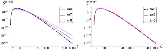
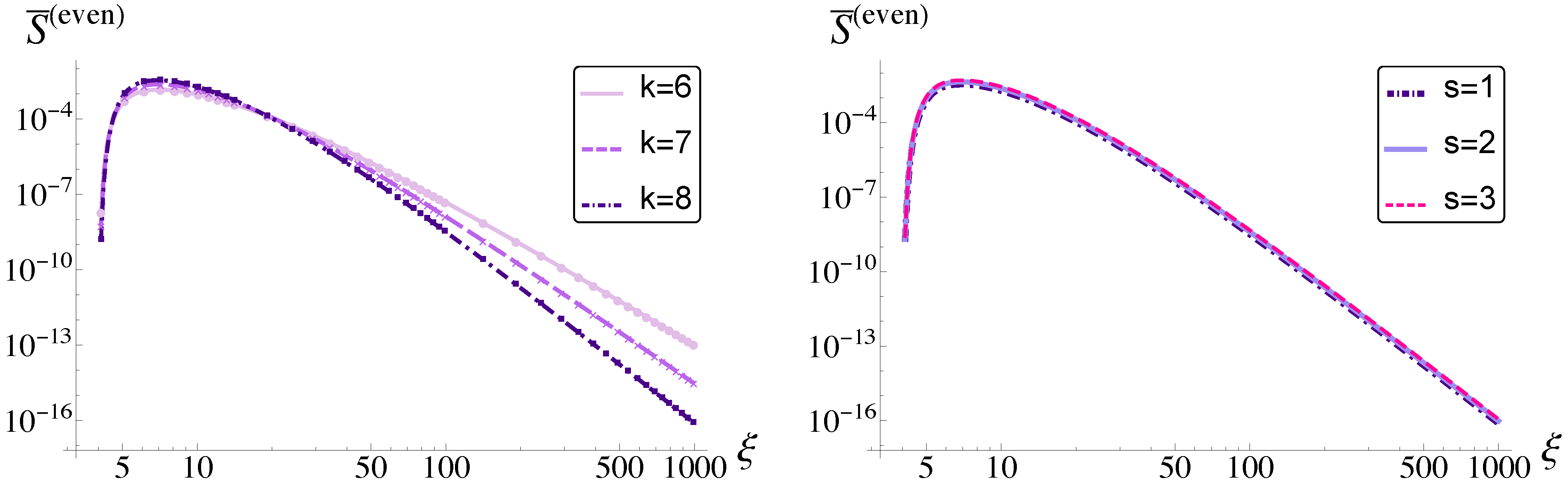
for different choices of the parameter space. The Figure 1 (left and right) shows the behavior of the normalized entropy density as a function of the dimensionless areal radius for a non-rotating kinetic gas. We observe from this plot that for larger values of the parameter k while keeping constant the parameter s, the configuration reaches maximum levels of entropy density at radii near the BH due to the polytropic ansatz contribution to the DF; increasing the parameter k favors more tightly bound, lower-energy particle trajectories, leading to a stronger concentration of particles and entropy density in the deeper regions of the gravitational potential, while simultaneously producing a steeper decay of the profiles at large radii. This behavior is observed in other related works [12]. In contrast, by varying s and keeping k constant, one finds that as s increases, the entropy density is more concentrated at radii nearer to the black hole. Since s controls the dependence of the DF on the inclination angle of the particle orbits, increasing s restricts the orbital population to a narrower range of inclinations. This produces a stronger concentration of entropy density around the preferred orbital region. As a result, the gas configuration becomes progressively more localized near the black hole. Similar behavior was observed previously for the particle density profiles, where increasing s led to more concentrated and disk-like configurations [12].
Figure 1.
Log-log plot showing the behavior of the normalized entropy density as a function of the dimensionless areal radius in the equatorial plane () in the non-rotating model. (Left panel): plot for different parameter values of and . (Right panel): plot for different parameter values of and .
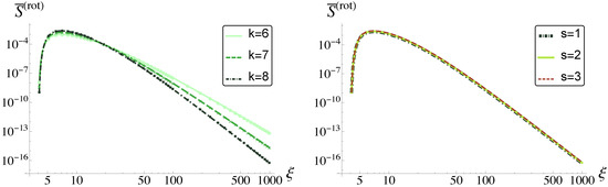
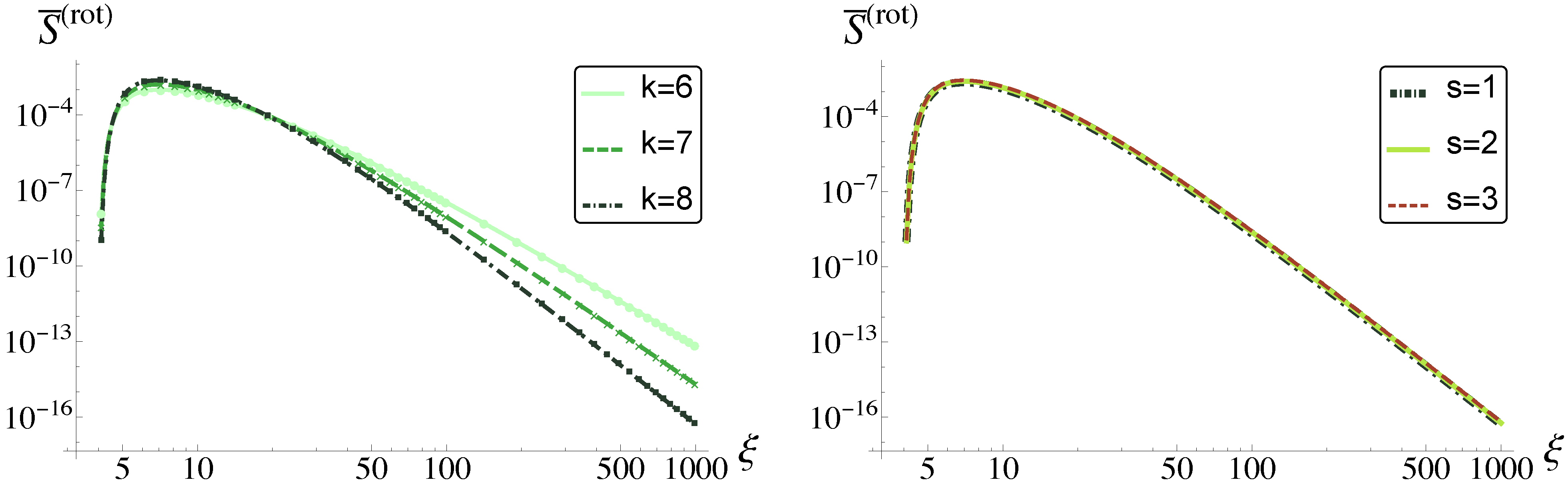
The behavior of S when varying the parameters k and s for a rotating gas is the same as for the non-rotating gas, as shown in Figure 2 (left and right). The physical origin of these trends is analogous to that of the non-rotating case, since the same energy-dependent polytropic factor controls the population of bound trajectories. Similarly, increasing s modifies the inclination-angle dependence of the DF.
Figure 2.
Log-log plot showing the behavior of the normalized entropy density as a function of the dimensionless areal radius in the equatorial plane () in the rotating model. (Left panel): plot for different parameter values of and . (Right panel): plot for different parameter values of and .
However, in the rotating model the invariant entropy density is not determined only by the temporal component of the entropy flux. In the rotating model, the invariant entropy density depends on both the temporal () and azimuthal contribution (). For the parameter values explored here, this contribution does not qualitatively alter the radial profile, which remains close to the non-rotating case. Nevertheless, it encodes the effect of the non-zero total angular momentum and produces a small but systematic reduction of the entropy density relative to the non-rotating model.
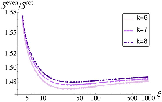
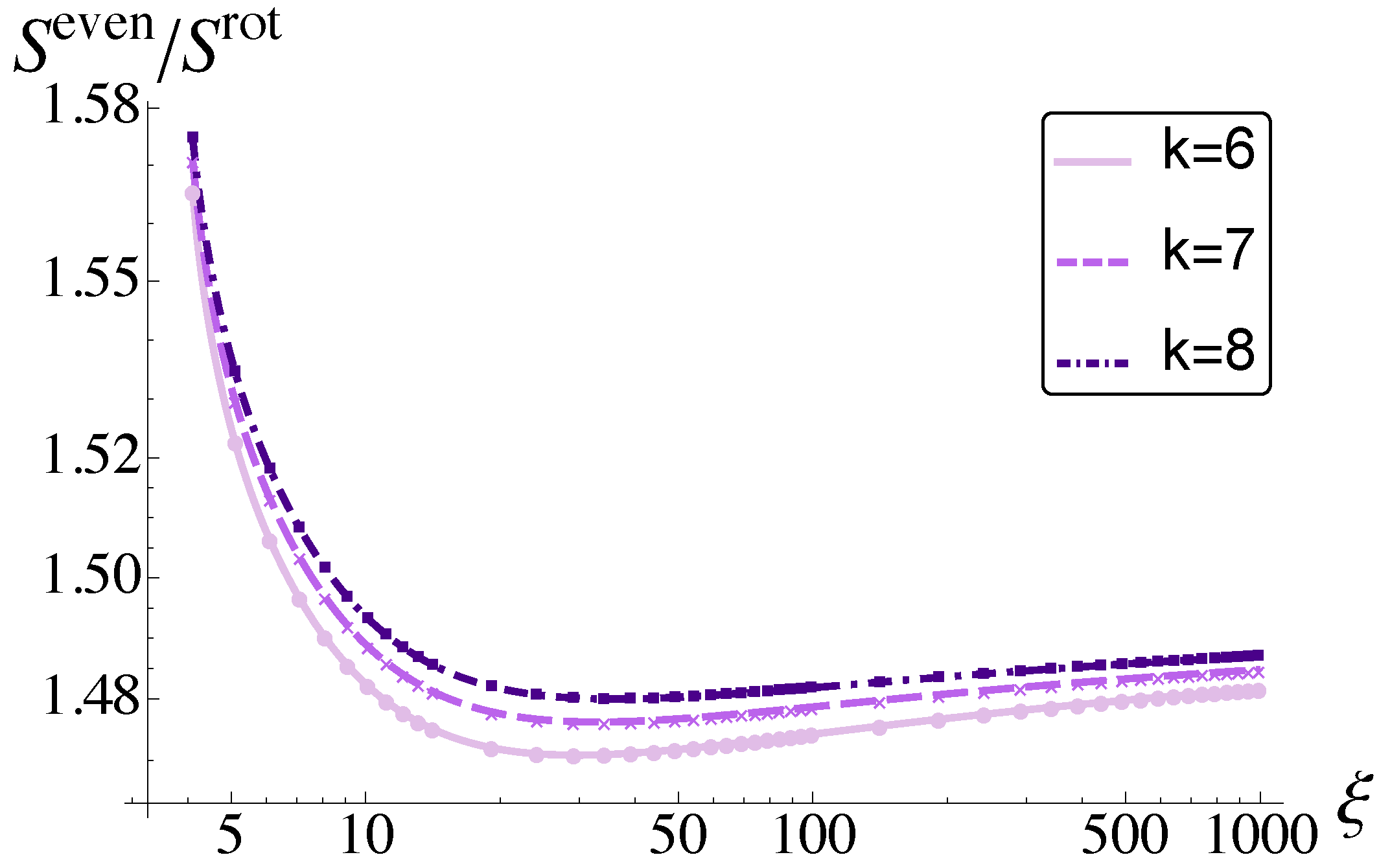
Comparing the entropy between the two models through the ratio , (as shown in Figure 3), we can make significant distinctions between the models, given different values of k and for different regions around the BH. The largest differences occur close to the black hole, where the effects of rotation on the orbital structure of the gas are expected to be more significant. For all explored values of the polytropic index parameter k, . This behavior is expected, as (43) yields a result from the difference between the two non-vanishing components of the entropy flux covector, while is directly proportional to the only non-vanishing term of the entropy flux for the non-rotating gas. Though the ratio of the entropy between the two models of gas always remains above the unity, the effect of the non-zero total angular momentum induced by the inclination angle model (33) implies a reduction in entropy density for this model. Also, for any value of k (on the equatorial plane), the ratio presents a minimum for radii closer to the BH. In this region, we expect that the entropy flux distributes in a less efficient way for the rotating gas than for its non-rotating counterpart. This suggests the system presents a greater sensitivity to rotational anisotropy due to the asymmetry in the total angular momentum induced by the rot inclination angle model1. Beyond this region, the ratio increases toward larger radii. This may indicate that the entropy reduction induced by the rotation of the configuration of gas is not exclusively an effect of the strong-gravity of the background, but rather a consequence of the behavior of the system due to phase-space mixing.
Figure 3.
Logarithmic plot of the relative difference with the normalized entropy density as a function of the dimensionless area radius in the equatorial plane () for and . The relative difference between the even and rotating models for different parameter space choices reveals a relativistic effect on the entropy density profiles invariant between the non-rotating and rotating models. The maximum relative difference occurs at the inner radius of the disk, while for intermediate radii it decreases to a minimum and then increases monotonically for large radii.
4. Principal Pressures and Anisotropy Parameter Behavior
As mentioned previously in Section 2, from the energy-momentum-stress tensor (4) we can obtain the principal pressures of the system, which are macroscopic observables of interest since they provide information about the gas’ behavior in terms of the velocity dispersion. Furthermore, the relationship between these principal pressures allows us to define an anisotropy parameter that quantifies how the random motions differ from the radial to the tangential direction, thus allowing us to infer a bias in the radial or tangential contributions over the kinetic gas.
The components of the pressure tensor for the non-rotating model are summarized as follows:
and the associated components for the rotating model are:
First, we will focus on the behavior of principal pressures, in which one can introduce the average pressure as follows
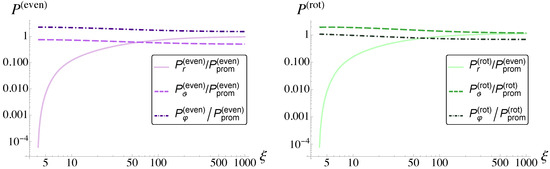
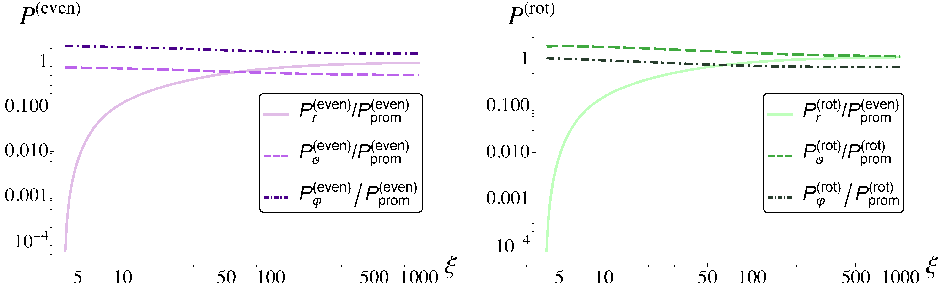
for both models (even) or (rot) correspondingly. Figure 4 shows the principal pressures (46) and (47) as functions of the dimensionless coordinate on the equatorial plane for the non-rotating and rotating models (left and right). We observe that in both models these pressures are different from each other in the region with radii near the BH, while for larger radii, the principal pressures on the radial and polar directions are always equal to each other.
Figure 4.
Log–log plot showing the behavior of the principal pressures (normalized by the average pressure ) as a function of the dimensionless radius in the equatorial plane (). For both panels (left and right), the parameter values are . (Left panel): plot for the non-rotating gas model. (Right panel): plot for the rotating gas model. Note that in these cases the three pressures are different from each other, with the radial pressure converging to polar pressure for large in both cases.
This behavior reflects the orbital nature of the particle motion. Near the black hole, particles in bound trajectories spend most of their time revolving around the central object, leading to larger tangential velocity dispersions and consequently larger angular pressures than radial pressure. As the radius increases, the gravitational influence weakens and the velocity dispersions become more similar in all directions, causing the principal pressures to approach a common value. This follows from the fact that the explicit expressions of (46) and (47) are different from each other; however, for large values of , the results agree with the non-relativistic limit discussed for similar models in [33]. On the other hand, the polar and azimuthal pressures are related by a factor depending on the s-parameter in the non-rotating case, while for the rotating case these principal pressures are related by an expression with a complex dependence on the polar angle; see Equations (36)–(39) and (42)–(46) in [12]. The behavior on the equatorial plane is shown in figures for both models for different values of the parameters .
Second, following the steps of the classic stellar-dynamical framework provided by Binney & Tremaine [10,34], anisotropy quantifies how a system’s random stellar motions differ between the radial direction (toward or away from the center) and the tangential directions (around the center). One commonly used definition is
where and are the one-dimensional velocity dispersions in the radial and combined tangential directions, respectively. When the stars orbits have no preferred direction, they are perfectly isotropic; positive indicates radially biased orbits (more radial excursions), while negative signals tangentially biased orbits (more circular motion).
To further explore the structure of these models with total (or zero) angular momentum, we introduce the anisotropy parameter as defined in [33] and in analogy to [10], as follows:
where the symbol ⊥ denotes the total contribution in the perpendicular motion associated with angular and azimuthal components and ‖ refers to the contribution in the radial motion. These are associated with the radial or tangential components of the pressure tensor.
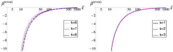
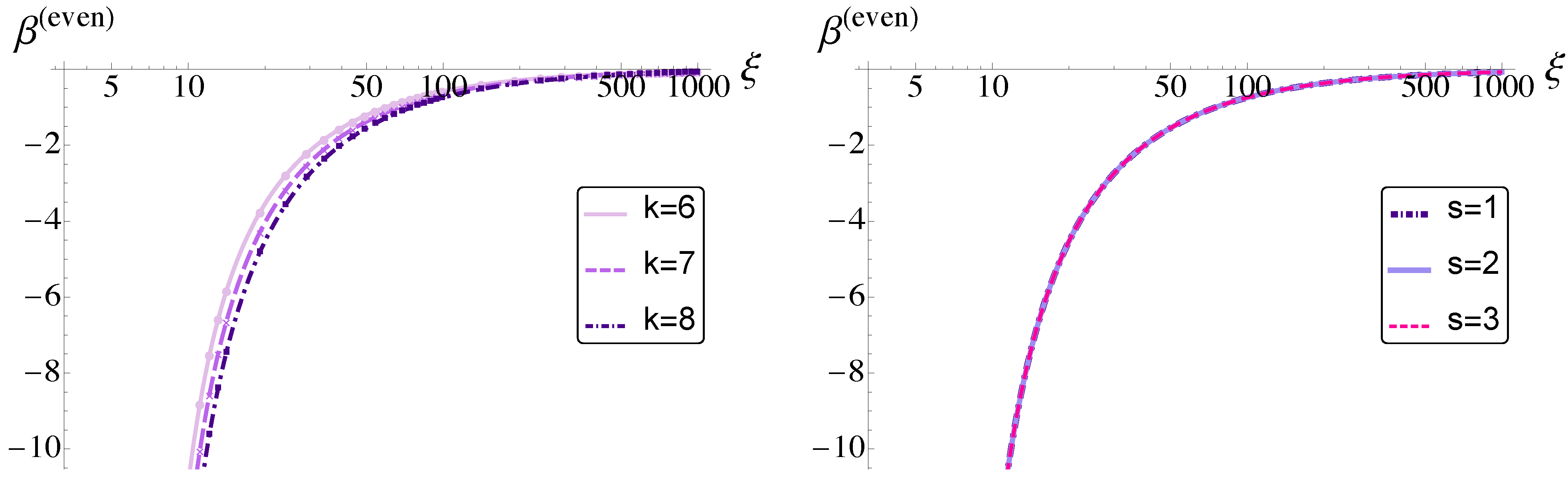
Figure 5 shows the behavior of the anisotropy parameter as a function of the dimensionless radius in the equatorial plane for the non-rotating gas model (zero angular momentum). In the left panel, it is observed that the anisotropy parameter exhibits a significant dependence on the value of k, especially in the intermediate region. For a fixed , the anisotropy decreases as k increases, indicating that, even in the absence of rotation, the choice of the parameter k modifies the structure of macroscopic observables in the non-collisional regime. In the right panel, unlike the case discussed before, the anisotropy parameter is practically independent of the value of s, exhibiting universal behavior for every . This suggests that, within the same non-rotating model, the distribution function is insensitive to the internal parameterization of s, while it does respond to variations in k.
Figure 5.
Log plot showing the behavior of the anisotropy parameter for the even model as a function of the dimensionless radius in the equatorial plane (). (Left panel): plot for the non-rotating gas model with parameter values and different k values. (Right panel): plot for the non-rotating gas model with parameter values and different s values.
We also observe that in both configurations of non-rotating gas, the anisotropy parameter exhibits negative values across the entire range of considered, indicating a preferential direction in the gas velocity distribution. This behavior is consistent with the non-collisional nature of the system, where the distribution function, depending solely on the motion constants, can generate systematic deviations from an isotropic distribution. Furthermore, it is observed that for large radii, the anisotropy parameter tends asymptotically to zero in all cases. This limit indicates that, at sufficient distances from the center, the gas recovers isotropic behavior regardless of the values of the parameters k and s. This trend is expected, since in external regions the gravitational field weakens and the particle trajectories become increasingly rectilinear and less influenced by the central geometry, leading to a more isotropic velocity distribution.
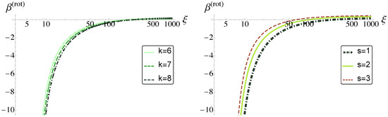
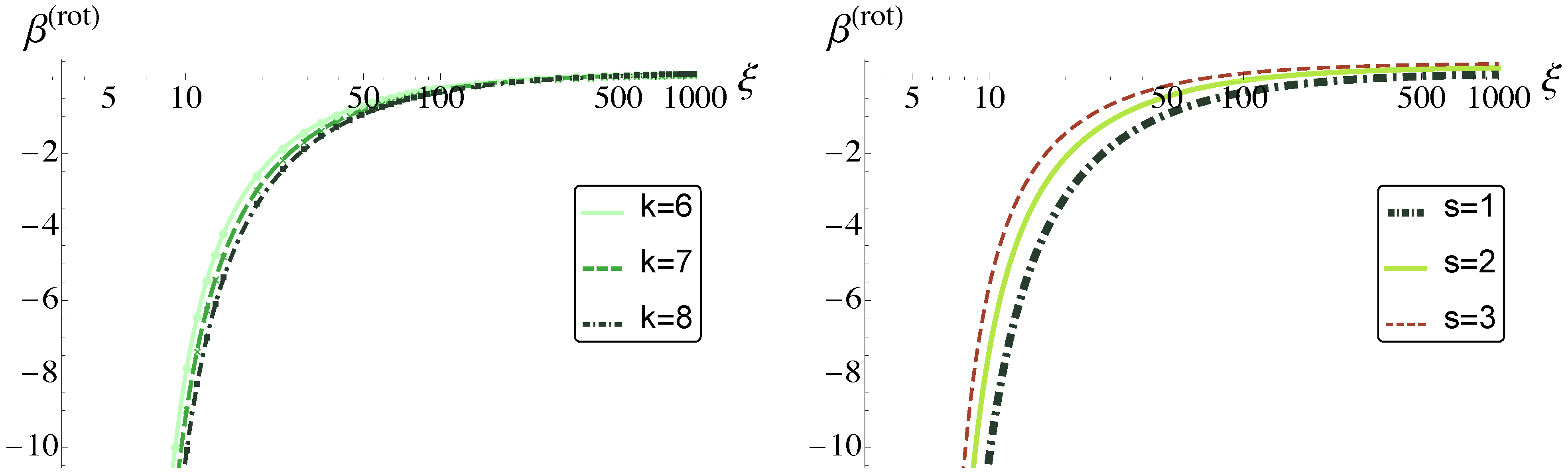
Figure 6 shows the behavior of the anisotropy parameter as a function of the dimensionless radius in the equatorial plane for the rotating gas model (non-zero total angular momentum). In the left panel, it can be seen that the anisotropy parameter exhibits a clear dependence on the value of k, particularly in the intermediate region. For a fixed , the anisotropy decreases as k increases, indicating that, in the rotating case, the choice of the parameter k significantly influences the macroscopic observables in the non-collisional regime. In the right panel, unlike the previous panel, the anisotropy parameter shows a moderate dependence on the value of s, especially for intermediate and large . As s increases, the anisotropy becomes slightly less negative, suggesting that the internal parameterization s does have an effect in the rotating model, unlike what was observed in the non-rotating case.
Figure 6.
Log plot showing the behavior of the anisotropy parameter for the rotating model as a function of the dimensionless radius in the equatorial plane (). (Left panel): plot for the rotating gas model with parameter values and different values of k. (Right panel): plot for the rotating gas model with parameter values and different values of s.
In contrast to the non-rotating model, in the rotating configuration the anisotropy parameter is not exclusively negative. As shown in Figure 6, for certain combinations of parameters and sufficiently large radii, the anisotropy parameter crosses zero and becomes positive. This indicates that the preferential direction in the gas velocity distribution can reverse in the presence of a total non-zero angular momentum, a feature that is absent in the non-rotating case. Furthermore, for large radii, the anisotropy parameter does not tend to zero but rather approaches a constant positive asymptotic value. This asymptotic limit depends on the parameter s (which increases with s), while it remains independent of k. In particular, positive values of the anisotropy parameter indicate that the radial velocity dispersion exceeds the tangential one, whereas negative values correspond to tangentially dominated motion. Therefore, the appearance of positive anisotropy in the rotating model suggests that the non-zero total angular momentum modifies the orbital population in such a way that radial motions become comparatively more important in some regions of the configuration.
A qualitative comparison between both models reveals several differences when contrasting the rotating case (Figure 6) with the non-rotating one (Figure 5). In the non-rotating model, the anisotropy was practically insensitive to variations in s and asymptotically vanished at large radii, indicating full isotropization. In contrast, the rotating model exhibits a clear dependence on s, particularly in the intermediate and large regions, and approaches a positive constant value scaled by s. The dependence on k, on the other hand, is present in both models, though with subtle differences in magnitude. Most notably, the rotating model allows the anisotropy parameter to become positive for certain parameter combinations and maintains a finite asymptotic anisotropy, whereas the non-rotating model remains strictly negative throughout the entire domain and fully isotropizes at infinity. These observations suggest that the presence of total non-zero angular momentum introduces a richer parametric structure in the description of the anisotropy, affecting not only the sign and magnitude of the macroscopic observables but also their asymptotic behavior.
To further enrich the discussion, in the next section we will introduce another macroscopic observable of interest: the kinetic temperature. In contrast to the thermal temperature discussed in Section 2, this kinetic temperature can be constructed directly from the particle density and principal pressures presented above.
5. Kinetic Temperature Behavior
Since we are studying the properties and behavior of the macroscopic observables of a non-collisional gas, we cannot speak of or refer to a thermal temperature of the gas in any sense. Such a thermal temperature is established for gases in thermodynamic equilibrium, which are a response to the frequent collisions between the individual particles of the system [35]. However, we are free to introduce a kinetic temperature through the ideal gas law, such that
with being the Boltzmann constant, the particle density (7), and the average pressure (48). Similar analyses of this macroscopic observable can be found in [27] for the relativistic regime and in [33] for the non-relativistic case. Figure 7 show the behavior of the kinetic temperature as a function of the dimensionless radius for the non-rotating gas model, while Figure 8 correspond to the rotating case.
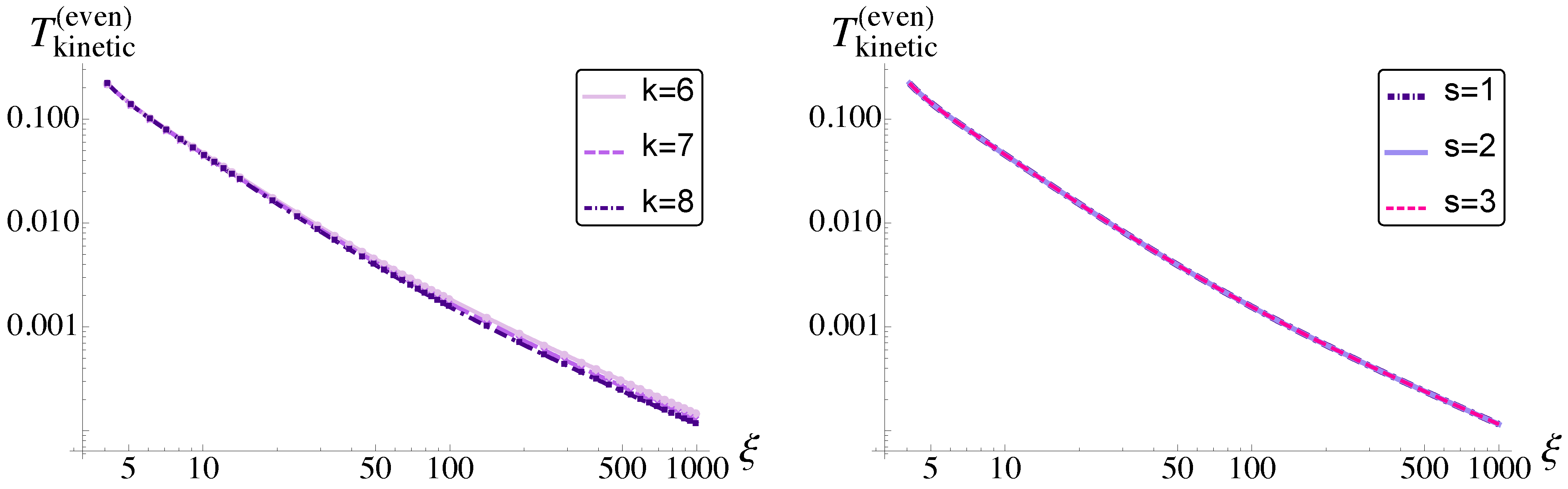
Figure 7.
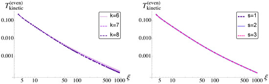
Log-log plot showing the behavior of the kinetic temperature for the non-rotating model as a function of the dimensionless radius in the equatorial plane (). (Left panel): plot for the non-rotating gas model with parameter values and . (Right panel): plot for the non-rotating gas model with parameter values and .
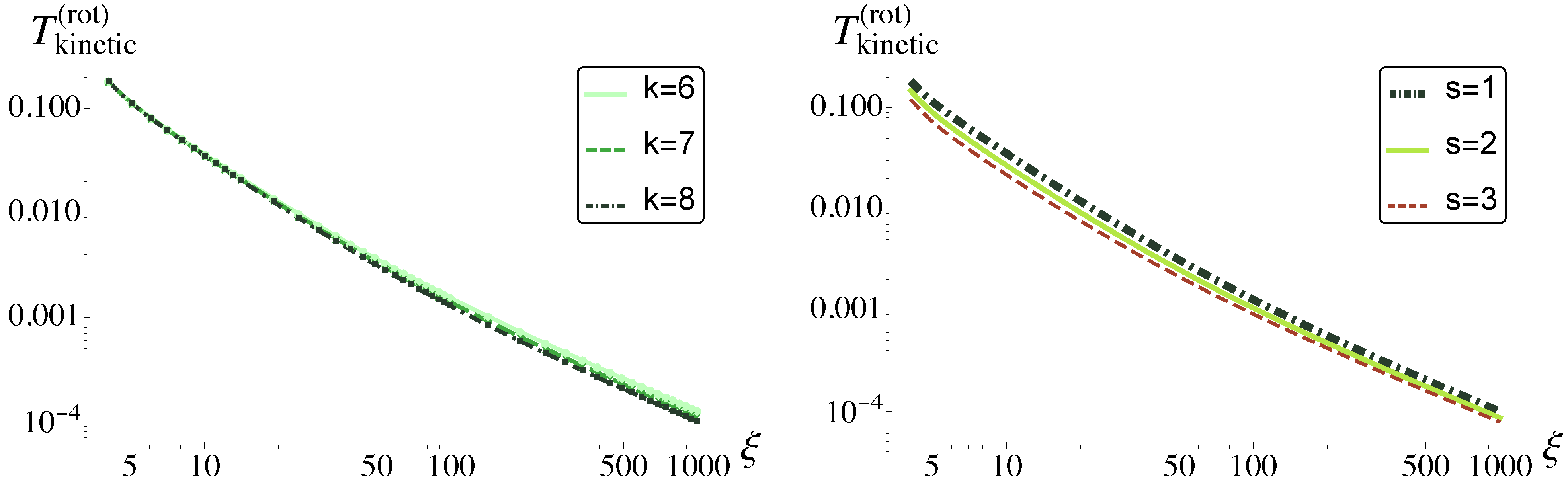
Figure 8.
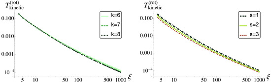
Log-log plot showing the behavior of the kinetic temperature for the rotating model as a function of the dimensionless radius in the equatorial plane (). (Left panel): plot for the rotating gas model with parameter values and . (Right panel): plot for the rotating gas model with parameter values and .
For the non-rotating model, the left panel of Figure 7 displays the kinetic temperature for fixed and varying . We observe a clear dependence on the parameter k: at a given radius , the temperature decreases as k increases. This sensitivity indicates that, even in the absence of angular momentum, the choice of k significantly affects the macroscopic thermal state of the gas. In contrast, the right panel of Figure 7 shows the kinetic temperature for fixed and varying . Here, the curves are practically indistinguishable for all , demonstrating that the temperature is insensitive to the internal parameter s in the non-rotating configuration. This behavior mirrors that observed for the anisotropy parameter, reinforcing the idea that s plays a minor role in the non-rotating regime.
For the rotating model, the situation is relatively different. The left panel of Figure 8 presents the kinetic temperature for fixed and varying . In this case, the dependence on k is weak; the curves almost overlap, with only marginal differences appearing at large (e.g., for , the value for is slightly lower than for and ). This suggests that in the presence of angular momentum, the kinetic temperature becomes nearly independent of k, unlike the non-rotating case. On the other hand, in the right panel, Figure 8 shows the temperature for fixed and varying . Here, the curves are again very similar, but a subtle dependence on s can be detected at the largest radii (e.g., at and yields a slightly higher value than or ). Thus, in the rotating model, the kinetic temperature exhibits a weak but non-zero sensitivity to both k and s, with the dependence on s becoming more noticeable in the asymptotic region. This contrasts with the non-rotating model, where only k has a significant effect, and highlights the richer parametric structure introduced by angular momentum.
An important implication arises from the behavior of the profiles shown in this article at larger radii. Since the Schwarzschild exterior is asymptotically flat, as , and the local orthonormal frame approaches the corresponding flat-spacetime frame. Therefore, the relativistic corrections associated with the Schwarzschild geometry disappear asymptotically. This limit, however, should not be interpreted as convergence toward a homogeneous gas in Minkowski spacetime. The configurations considered here are localized collisionless steady states made of particles on bound geodesics and normalized to have finite total particle number. When , the energy cutoff gives rise to configurations with finite radial extent. In the limiting case , the support may extend to arbitrarily large radii, but the local macroscopic observables decay as , consistently with the finite-mass conditions imposed on the DF [27,33]. Thus, the flat-spacetime limit is recovered in the sense that the background geometry and the local momentum parametrization approach their special-relativistic form, while the localized particle density, entropy density, pressure components, and average pressure vanish asymptotically. Dimensionless ratios constructed from these quantities, such as the anisotropy parameter, may nevertheless approach finite limits because the dominant radial decay cancels between numerator and denominator.
Finally, a natural question is how these results would contrast with those obtained from a hydrodynamic description, where frequent collisions enforce local thermodynamic equilibrium. In such a regime, anisotropies are rapidly erased, pressures become isotropic, and the temperature follows a different radial profile, typically governed by an equation of state. Moreover, the effects of angular momentum in a collisional fluid are transmitted through collective motions rather than through the distribution function itself. Comparing both approaches highlights the distinctive signatures of collisionless dynamics: persistent anisotropies, sensitivity to the parameters, k and s. The following discussion in Section 6 outlines some qualitative points of contrast, helping to contextualize the kinetic results and to underscore the importance of the appropriate model choice depending on the physical regime of interest.
6. Qualitative Comparison with a Hydrodynamic Model
To characterize the macroscopic behavior of the kinetic model proposed in this article, we compare its predictions with those of a relativistic fluid model, such as the Polish doughnut model [23]. For this hydrodynamic model, we assume an adiabatic fluid in local thermodynamic equilibrium that obeys the ideal gas equation . The polytropic equation of state is given by where K is a constant and is the adiabatic index subject to . This adiabatic index is related to the polytropic index k by (see [10] and (31)). Here, the particle density n, temperature T, and pressure P are related to the specific enthalpy h, (see for example Appendix E in [27] for more details) by
where is the average rest mass per particle.
For a polytropic flow, the specific entropy per baryon remains constant throughout the fluid if the polytropic index coincides with the gas adiabatic index, which is precisely our assumption. Using the first law of thermodynamics and the previous relations, one can derive an expression for the entropy. For a relativistic ideal gas, the specific entropy s is related to K and by
For a Polish doughnut with a polytropic equation of state, the entropy is uniform throughout the torus (isoentropic flow). This implies , which is consistent with the barotropic fluid assumption. In its original and simplest formulation, the Polish doughnut model assumes that the disc matter can be described by the energy-momentum stress tensor of a perfect fluid. In such a fluid, the pressure is isotropic, meaning it is the same in all directions (radial, azimuthal, and vertical). Consequently, there is no intrinsic anisotropy parameter (as in the kinetic model), as the system is, by definition, isotropic in the fluid’s rest frame. This assumption greatly simplifies the equilibrium equations (the relativistic Euler equation) and allows for the construction of analytical solutions for the shape and structure of the torus [23].
Furthermore, to perform a graphical qualitative comparison, we adjust the adiabatic index with the polytropic index k, so that the fluid and kinetic configurations are described with the same adiabatic index
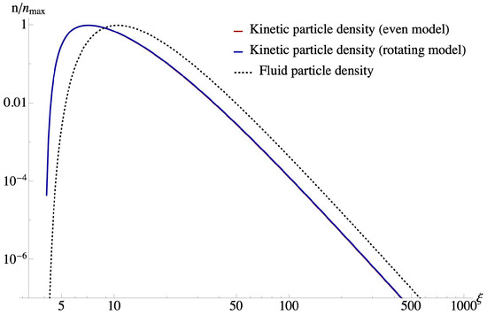
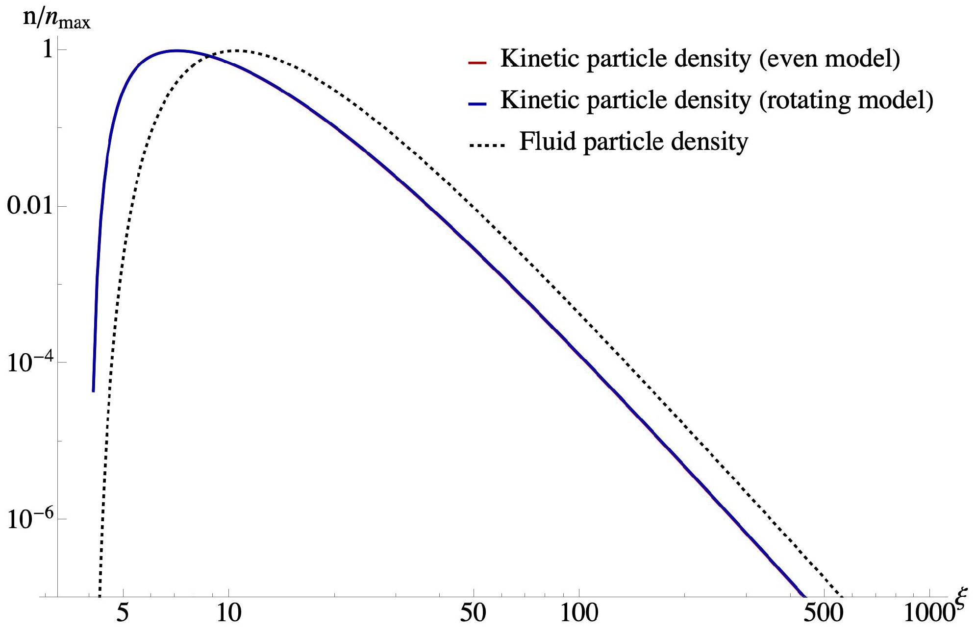
The Figure 9 compares the normalized particle density profiles obtained from the kinetic and fluid dynamic models. A clear difference between the two descriptions lies in the radial position of the density maximum. For all values of the parameters considered, the kinetic model predicts a peak located closer to the central object than the corresponding fluid model. Even so, both models show the same general radial behavior: the density increases from the lower limit to a maximum and then decreases as the radius increases. On the other hand, the rotating and non-rotating kinetic models produce almost identical normalized density profiles, with no visible differences between them. This general behavior is consistent with the results reported in [12], where it was also observed that the normalized density profiles exhibited the same qualitative trends for a different family of kinetic models.
Figure 9.
Normalized particle-density profiles as functions of the radial coordinate for the fluid and kinetic descriptions. The dotted curve represents the fluid model with , while the solid curves correspond to the rotating and non-rotating kinetic solutions evaluated with .
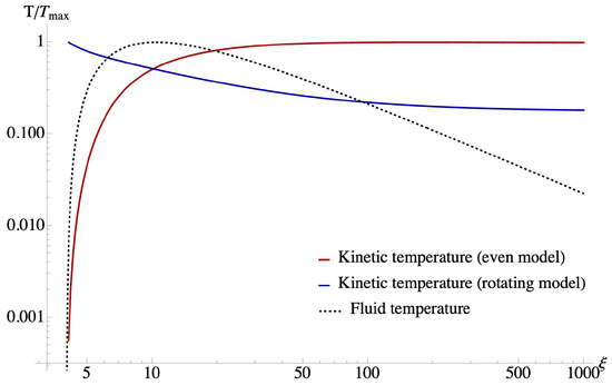
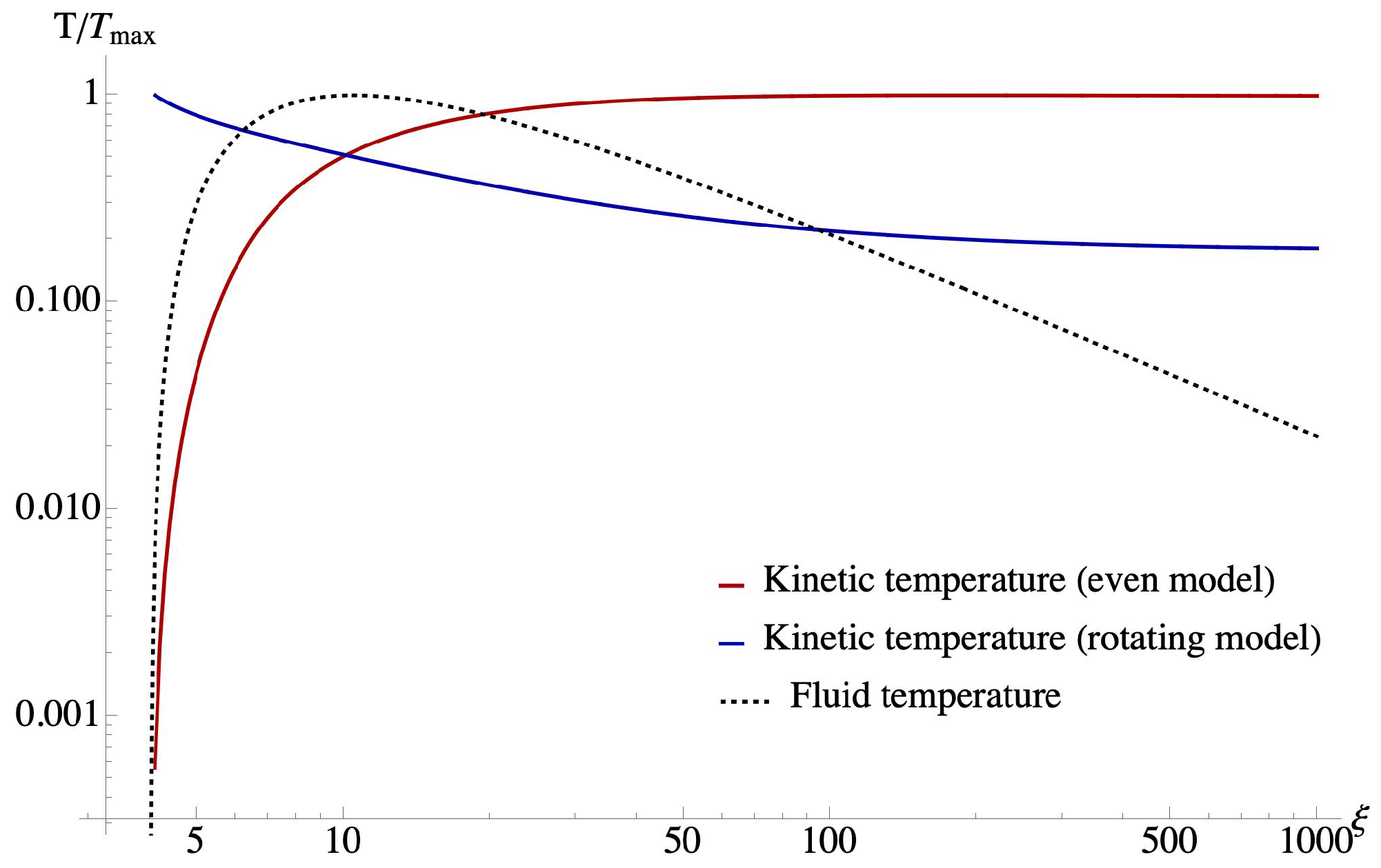
Figure 10 shows that the relationship between kinetic and fluid temperatures is markedly different from that found for particle density. Unlike density profiles, temperature distributions do not follow the same radial behavior. The locations of their maxima differ, and changes in kinetic temperature are not accompanied by similar variations in fluid temperature. As a result, the two models predict distinct temperature profiles across the radial domain. An additional feature of current kinetic models is that, as the radial coordinate increases, both kinetic temperature profiles approach constant asymptotic values, while the fluid temperature continues to decrease. This asymptotic behavior was not observed in previously analyzed kinetic models, highlighting a qualitative difference between the two families of collisionless gas models.
Figure 10.
Radial dependence of the normalized temperature predicted by the fluid and kinetic descriptions. The dotted curve corresponds to the fluid solution computed with an adiabatic index , whereas the solid curves represent the rotating and non-rotating kinetic models for .
In the collisionless kinetic models studied previously [11,12,22,27,33], and in the present work, temperature is interpreted as a measure of the local velocity dispersion and not as a thermodynamic temperature. Its radial dependence arises because the set of bound orbits traversed by each position changes with the radius, modifying the momenta of the distribution and, therefore, the local kinetic pressures and temperatures. The kinetic temperatures introduced in the Vlasov models must be interpreted with care, since, unlike a thermodynamic temperature, they are defined by appropriate momenta of the distribution function and, therefore, quantify the local velocity dispersion of the particle distribution. In stationary configurations composed of bounded geodesics, the set of trajectories that contribute to the distribution generally varies with position, naturally giving rise to radial profiles for the kinetic temperatures. Consequently, a spatially varying kinetic temperature does not necessarily imply local thermal equilibrium or the existence of heat transport in the usual thermodynamic sense. Although relativistic kinetic theory provides a well-established description of heat flow and other dissipative processes in collisional gases near equilibrium [36], collisionless accretion corresponds to the opposite regime, where collisions are negligible and energy transport must be analyzed directly from the momenta of the distribution function.
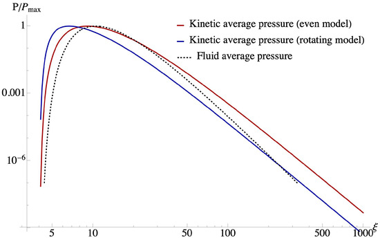
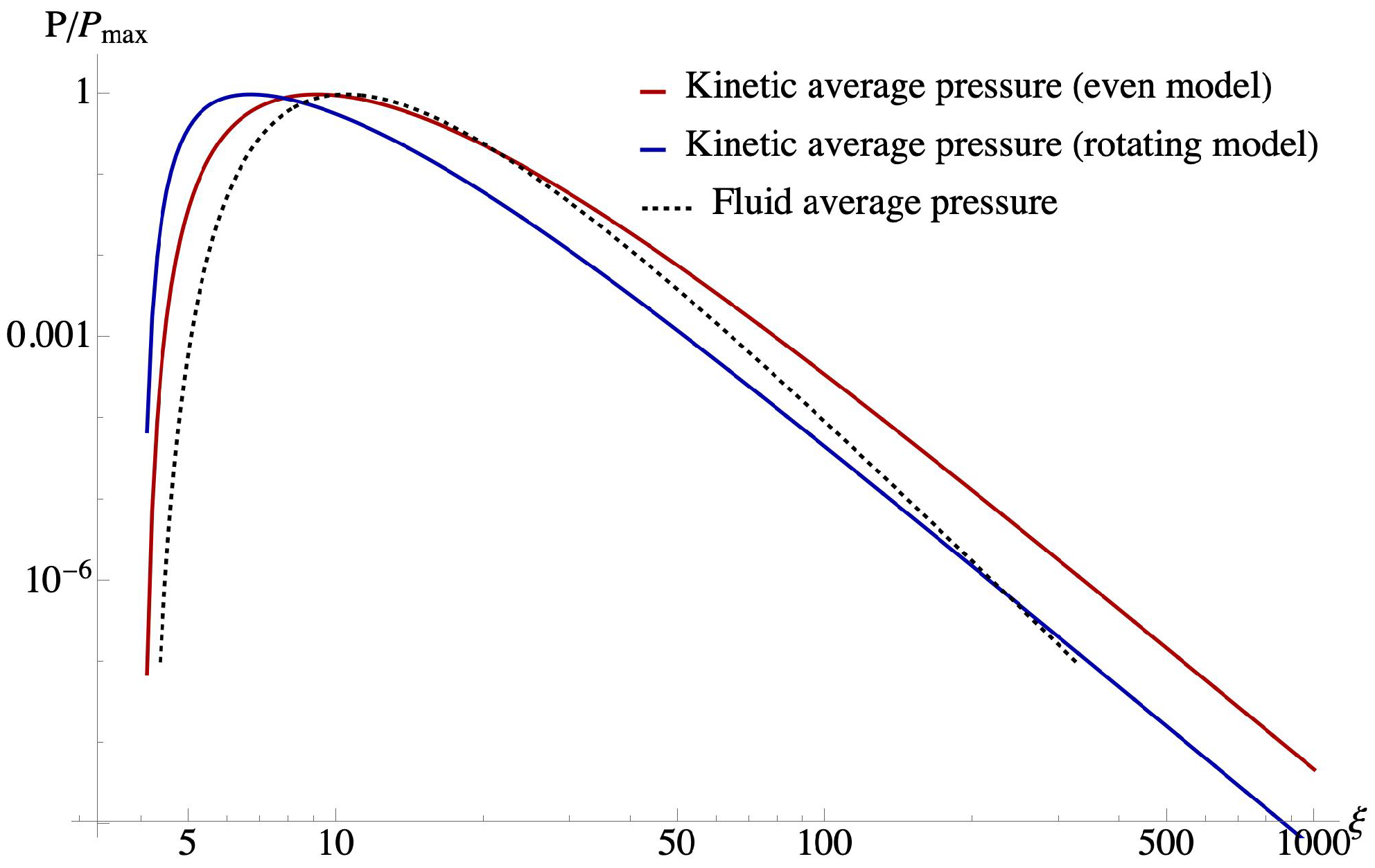
Figure 11 shows the behavior of the average pressure as a function of the dimensionless radius for the three cases under consideration: the kinetic even (non-rotating) model, the kinetic rotating model, and the fluid (hydrodynamic) model. All three curves exhibit virtually identical behavior across the entire radial domain. For small radii the pressure increases, while in the intermediate region it reaches a maximum. Beyond large radii, the pressure decreases sharply, approaching zero. The striking agreement between the kinetic models and the fluid description indicates that, despite the fundamentally different underlying dynamics between collisionless and collisional systems, the average pressure is an observable that remains insensitive to both the presence of angular momentum and the detailed kinetic parameters. This suggests that the average pressure is primarily determined by the overall density distribution and gravitational potential, rather than by the specific microscopic state of the gas.
Figure 11.
Normalized radial profiles of the average pressure for the fluid and kinetic models. The dotted curve represents the fluid solution with an adiabatic index , whereas the solid curves correspond to the rotating and non-rotating kinetic configurations computed with .
Based on the results shown so far, the next section presents the conclusions derived from this study.
7. Conclusions
In this article, we have studied the morphological properties of a collisionless relativistic kinetic gas around a Schwarzschild black hole, described by a one-particle distribution function that depends on the constants of motion through an ansatz motivated by the inclination angle of bound orbits and a generalized polytropic energy dependence [11,12]. By considering two distinct models for the angular dependence, the even model describing a non-rotating gas and the rot model describing a rotating one, we have analyzed and compared the behavior of key macroscopic observables, including the entropy density, the anisotropy parameter, the kinetic temperature, and the average pressure.
We have derived explicit expressions for the components of the entropy covector field for both models, including the angular integrals provided in Appendix A that determine their dependence on the polar angle. The normalized invariant entropy density, defined in Equation (45) and shown in Figure 1 and Figure 2, reveals that configurations with larger values of the polytropic parameter k exhibit higher entropy density levels, while increasing the angular parameter s concentrates the entropy more sharply. A novel result is the entropic contrast between models presented in Figure 3: the ratio is strictly greater than unity throughout the entire radial domain, demonstrating that the presence of angular momentum systematically reduces the invariant entropy density. This ratio exhibits a minimum at intermediate radii () and increases monotonically toward large distances, indicating that the entropy suppression induced by rotation persists even in the asymptotic region and is not merely a strong-field effect.
The anisotropy parameter, defined from the principal pressures, shows markedly different behavior between the two models, as illustrated in Figure 5 and Figure 6. In the non-rotating case, it is always negative, insensitive to variations in s, and tends asymptotically to zero at large radii, indicating complete isotropization far from the black hole. In contrast, the rotating model exhibits a clear dependence on both parameters: it decreases with increasing k and shows a moderate sensitivity to s, particularly at intermediate and large . Most notably, the anisotropy parameter in the rotating model can cross zero and become positive for certain parameter combinations, and it approaches a constant positive asymptotic value that depends exclusively on s while remaining independent of k. This constitutes a key finding: rotation introduces a persistent residual anisotropy that does not vanish even at large distances, fundamentally distinguishing rotating from non-rotating collisionless gases.
The kinetic temperature, constructed from the ideal gas law using the average pressure and the particle density, exhibits contrasting parametric sensitivities, as shown in Figure 7 and Figure 8. In the non-rotating model, it depends significantly on k but is practically insensitive to s, mirroring the behavior of the anisotropy parameter. In the rotating model, however, the temperature shows weak sensitivity to both parameters, with a subtle dependence on s becoming noticeable only at the largest radii. This indicates that angular momentum affects the anisotropy and modulates the thermal response of the gas, smoothing out the parametric dependence observed in the non-rotating case.
Finally, we have performed a systematic qualitative comparison between our kinetic models and a relativistic fluid description, specifically the Polish doughnut model [23] with an adiabatic index matched to the kinetic polytropic parameter via Equation (54). The results, summarized in Figure 9, Figure 10 and Figure 11, provide a clear qualitative picture of the similarities and differences between the two descriptions. The particle density profiles show global morphological agreement between kinetic and fluid models, both increasing from large radii to a maximum and then decreasing inward; however, the radial position of the maximum is systematically shifted between the two descriptions, a discrepancy that persists regardless of the choice of parameters k and s. The kinetic temperature displays no correlation with the fluid temperature: the radial variations, maxima locations, and overall profile shapes are qualitatively different. Remarkably, the average pressure exhibits a similar behavior across all models (kinetic non-rotating, kinetic rotating, and fluid) throughout the entire radial domain.
In summary, this work provides a comprehensive characterization of the macroscopic observables of collisionless relativistic kinetic gases around Schwarzschild black holes, revealing how the inclusion of angular momentum qualitatively modifies the entropy, anisotropy, and temperature profiles. The anisotropy in the rotating model, the construction of the entropy flux covector, and the contrasting behavior of the kinetic temperature compared to fluid descriptions constitute original contributions that extend previous studies. These findings highlight the importance of a kinetic treatment for collisionless systems in strong gravitational fields and open the door to further investigations, such as the inclusion of weak collisions, self-gravity effects, or extensions to other spacetime backgrounds admitting bound orbits.
Author Contributions
Conceptualization, C.E.G. and R.J.R.R.; Methodology, C.E.G., D.M.M. and R.J.R.R.; Software, C.E.G., D.M.M. and R.J.R.R.; Validation, C.E.G., D.M.M. and R.J.R.R.; Formal analysis, C.E.G., D.M.M. and R.J.R.R.; Investigation, C.E.G., D.M.M. and R.J.R.R.; Resources, C.E.G. and R.J.R.R.; Writing—original draft, C.E.G., D.M.M. and R.J.R.R.; Writing—review and editing, C.E.G., D.M.M. and R.J.R.R.; Supervision, C.E.G.; project administration, C.E.G. All authors have read and agreed to the published version of the manuscript.
Funding
This research received no external funding.
Data Availability Statement
The original contributions presented in this study are included in the article. Further inquiries can be directed to the corresponding author.
Acknowledgments
We thank Olivier Sarbach for fruitful comments and discussions throughout this work. C. Gabarrete acknowledges support from SECIHTI through the project Hyperbolic and causal evolution for first-order dissipative relativistic plasmas in gradients: microscopic foundation and applications (CBF-2025-G-1626). The analytical expressions for the angle integrals in Equations (A4) and (A6) were initially proposed using artificial intelligence tools, as they could not be evaluated via conventional analytical methods. These expressions were subsequently verified through numerical integration in Wolfram Mathematica 14.2 [32], showing convergence to three significant figures. For the purposes of this work, this level of precision is considered sufficient. The authors confirm the validity of the results presented and assume full responsibility for the work.
Conflicts of Interest
The authors declare no conflicts of interest.
Appendix A. Performing Angular Integrals in Kinetic Models
The functions that appear in the components of the entropy flux covector field, which determines the angular dependence of the macroscopic observables in the non-rotating or rotating models explored in this article, are defined as follows:
Here is the generalized hypergeometric function and denotes the digamma function (see [37]) defined by
Note
| 1 | The behavior described for the equatorial plane () persists throughout almost the entire configuration for all . However, as the polar angle approaches the poles ( or ), the behavior changes: the ratio between the non-rotating (32) and rotating (33) configurations reaches a maximum because the non-rotating distribution function tends to zero at the poles, allowing the rotating contribution to become dominant. |
References
- Cercignani, C.; Kremer, G. The Relativistic Boltzmann Equation: Theory and Applications; Birkhäuser: Basel, Switzerland, 2002. [Google Scholar]
- Sarbach, O.; Zannias, T. Relativistic kinetic theory: An Introduction. AIP Conf. Proc. 2013, 1548, 134–155. [Google Scholar] [CrossRef] [Scilit]
- Sarbach, O.; Zannias, T. Tangent bundle formulation of a charged gas. AIP Conf. Proc. 2014, 1577, 192–207. [Google Scholar] [CrossRef] [Scilit]
- Sarbach, O.; Zannias, T. The geometry of the tangent bundle and the relativistic kinetic theory of gases. Class. Quantum Gravity 2014, 31, 085013. [Google Scholar] [CrossRef] [Scilit]
- Akiyama, K. et al. [Event Horizon Telescope Collaboration] First M87 Event Horizon Telescope Results. I. The Shadow of the Supermassive Black Hole. Astrophys. J. Lett. 2019, 875, L1. [Google Scholar] [CrossRef] [Scilit]
- Akiyama, K. et al. [Event Horizon Telescope Collaboration] First M87 Event Horizon Telescope Results. IV. Imaging the Central Supermassive Black Hole. Astrophys. J. Lett. 2019, 875, 52. [Google Scholar] [CrossRef] [Scilit]
- Akiyama, K. et al. [Event Horizon Telescope Collaboration] First Sagittarius A* Event Horizon Telescope Results. I. The Shadow of the Supermassive Black Hole in the Center of the Milky Way. Astrophys. J. Lett. 2022, 930, L12. [Google Scholar] [CrossRef] [Scilit]
- Akiyama, K. et al. [Event Horizon Telescope Collaboration] First Sagittarius A* Event Horizon Telescope Results. III. Imaging of the Galactic Center Supermassive Black Hole. Astrophys. J. Lett. 2022, 930, 64. [Google Scholar] [CrossRef] [Scilit]
- Kunz, M.; Stone, J.; Quataert, E. Magnetorotational Turbulence and Dynamo in a Collisionless Plasma. Phys. Rev. Lett. 2016, 117, 235101. [Google Scholar] [CrossRef] [Scilit] [PubMed]
- Binney, J.; Tremaine, S. Galactic Dynamics, 2nd ed.; Princeton University Press: Princeton, NJ, USA, 2008. [Google Scholar]
- Gabarrete, C.; Sarbach, O. Kinetic gas disks surrounding Schwarzschild black holes. Acta Phys. Pol. B Proc. Suppl. 2022, 15, 1-A10. [Google Scholar] [CrossRef] [Scilit]
- Gabarrete, C.; Raudales, R. Rotating kinetic gas disk morphology surrounding a Schwarzschild black hole. Class. Quantum Gravity 2026, 43, 095012. [Google Scholar] [CrossRef] [Scilit]
- Ames, E.; Andréasson, H.; Logg, A. On Axisymmetric and Stationary Solutions of the Self-Gravitating Vlasov System. Class. Quantum Gravity 2016, 32, 155008. [Google Scholar] [CrossRef] [Scilit]
- Ames, E.; Andréasson, H.; Logg, A. Cosmic String and Black Hole Limits of Toroidal Vlasov Bodies in General Relativity. Phys. Rev. D 2019, 99, 024012. [Google Scholar] [CrossRef] [Scilit]
- Mach, P.; Momennia, M.; Sarbach, O. Bondi-type accretion onto a Kerr black hole in the kinetic regime. Phys. Rev. D 2026, 113, L041505. [Google Scholar] [CrossRef] [Scilit]
- Mach, P.; Momennia, M.; Sarbach, O. Accretion of a Vlasov gas by a Kerr black hole. Phys. Rev. D 2026, 113, 044068. [Google Scholar] [CrossRef] [Scilit]
- Liu, Y. A discussion on the symmetry of relativistic Vlasov gas and its accretion in Kerr-Newman black hole. arXiv 2025, arXiv:2506.08341. [Google Scholar] [CrossRef] [Scilit]
- Jüttner, F. Maxwell’s law of speed distribution in the theory of relativity. Ann. Phys. 1911, 34, 856–882. [Google Scholar]
- Jüttner, F. The dynamics of an inert gas in the theory of relativity. Ann. Phys. 1911, 35, 145–161. [Google Scholar]
- Mach, P.; Odrzywołek, A. Accretion of the relativistic Vlasov gas onto a moving Schwarzschild black hole: Exact solutions. Phys. Rev. D 2021, 103, 024044. [Google Scholar] [CrossRef] [Scilit]
- Mach, P.; Odrzywołek, A. Accretion of Dark Matter onto a Moving Schwarzschild Black Hole: An Exact Solution. Phys. Rev. Lett. 2021, 126, 101104. [Google Scholar] [CrossRef] [Scilit] [PubMed]
- Gamboa, A.; Gabarrete, C.; Domínguez-Fernández, P.; Núñez, D.; Sarbach, O. Accretion of a Vlasov gas onto a black hole from a sphere of finite radius and the role of angular momentum. Phys. Rev. D 2021, 104, 083001. [Google Scholar] [CrossRef] [Scilit]
- Rezzolla, L.; Zanotti, O. Relativistic Hydrodynamics; Oxford University Press: Oxford, UK, 2013. [Google Scholar]
- Synge, J. Relativity: The Special Theory; Elsevier Science: Amsterdam, The Netherlands, 1956. [Google Scholar]
- Acuña-Cárdenas, R.; Gabarrete, C.; Sarbach, O. An introduction to the relativistic kinetic theory on curved spacetimes. Gen. Relativ. Gravit. 2022, 54, 23. [Google Scholar] [CrossRef] [Scilit]
- Israel, W. Relativistic Kinetic Theory of a Simple Gas. J. Math. Phys. 1963, 4, 1163–1181. [Google Scholar] [CrossRef] [Scilit]
- Gabarrete, C.; Sarbach, O. Axisymmetric, stationary collisionless gas configurations surrounding Schwarzschild black holes. Class. Quantum Gravity 2023, 40, 055012. [Google Scholar] [CrossRef] [Scilit]
- Rioseco, P.; Sarbach, O. Accretion of a relativistic, collisionless kinetic gas into a Schwarzschild black hole. Class. Quantum Gravity 2017, 34, 095007. [Google Scholar] [CrossRef] [Scilit]
- Rioseco, P.; Sarbach, O. Spherical steady-state accretion of a relativistic collisionless gas into a Schwarzschild black hole. J. Phys. Conf. Ser. 2017, 831, 012009. [Google Scholar] [CrossRef] [Scilit]
- Rioseco, P.; Sarbach, O. Phase space mixing in the equatorial plane of a Kerr black hole. Phys. Rev. D 2018, 98, 124024. [Google Scholar] [CrossRef] [Scilit]
- Rioseco, P.; Sarbach, O. Phase Space Mixing of a Vlasov Gas in the Exterior of a Kerr Black Hole. Commun. Math. Phys. 2024, 405, 105. [Google Scholar] [CrossRef] [Scilit]
- Wolfram Research, Inc. Mathematica, Version 14.2; Wolfram Research, Inc.: Champaign, IL, USA, 2024; License number 8807-2525.
- Gabarrete, C.; Sarbach, O. Axisymmetric, stationary collisionless gas clouds trapped in a Newtonian potential. Class. Quantum Gravity 2023, 40, 055013. [Google Scholar] [CrossRef] [Scilit]
- Chemin, L. A mass-velocity anisotropy relation in galactic stellar disks. Astron. Astrophys. 2018, 618, 19. [Google Scholar] [CrossRef] [Scilit]
- Israel, W. Event Horizons in Static Vacuum Space-Times. Phys. Rev. 1967, 164, 1776–1779. [Google Scholar] [CrossRef] [Scilit]
- Gabarrete, C.; García-Perciante, A.L.; Sarbach, O. Kinetic theory for a relativistic charged gas: Mathematical foundations of the hydrodynamic limit and first-order results within the projection method. J. Non-Equilib. Thermodyn. 2026, 51, 459–492. [Google Scholar] [CrossRef] [Scilit]
- Digital Library of Mathematical Functions, National Institute of Standards and Technology (NIST). Available online: https://dlmf.nist.gov/ (accessed on 15 April 2026).
Disclaimer/Publisher’s Note: The statements, opinions and data contained in all publications are solely those of the individual author(s) and contributor(s) and not of MDPI and/or the editor(s). MDPI and/or the editor(s) disclaim responsibility for any injury to people or property resulting from any ideas, methods, instructions or products referred to in the content. |
© 2026 by the authors. Licensee MDPI, Basel, Switzerland. This article is an open access article distributed under the terms and conditions of the Creative Commons Attribution (CC BY) license.