Real-Time Vehicle Detection Framework Based on the Fusion of LiDAR and Camera

Abstract

Vehicle detection is essential for driverless systems. However, the current single sensor detection mode is no longer sufficient in complex and changing traffic environments. Therefore, this paper combines camera and light detection and ranging (LiDAR) to build a vehicle-detection framework that has the characteristics of multi adaptability, high real-time capacity, and robustness. First, a multi-adaptive high-precision depth-completion method was proposed to convert the 2D LiDAR sparse depth map into a dense depth map, so that the two sensors are aligned with each other at the data level. Then, the You Only Look Once Version 3 (YOLOv3) real-time object detection model was used to detect the color image and the dense depth map. Finally, a decision-level fusion method based on bounding box fusion and improved Dempster–Shafer (D–S) evidence theory was proposed to merge the two results of the previous step and obtain the final vehicle position and distance information, which not only improves the detection accuracy but also improves the robustness of the whole framework. We evaluated our method using the KITTI dataset and the Waymo Open Dataset, and the results show the effectiveness of the proposed depth completion method and multi-sensor fusion strategy.

1. Introduction

Autonomous vehicles can improve the efficiency and safety of transportation systems, and have become the main topic of future traffic development. In the study of autonomous vehicles, vehicle detection is the key to ensure safe driving of autonomous vehicles. Autonomous vehicles are usually equipped with many different sensors to sense environmental information, such as camera, light detection and ranging (LiDAR), radar, ultrasonic radar, and so on. Among the above sensors, the camera and LiDAR have become the most commonly used sensors in the object detection field due to their superior performance.

The camera is widely used because of its high resolution. There has been a lot of literature on image-based object detection. In recent years, with the continuous development of deep learning, many scholars have introduced convolutional neural networks (CNNs) into the field of object detection and achieved excellent results. We usually divide the methods of object detection based on deep learning into two categories, the two-stage method and the one-stage method. The two-stage object detection method is also called the region-based object detection method. The classic models include regions with CNN features (R-CNN) [1], spatial pyramid pooling network (SSP-Net) [2], fast R-CNN [3], faster R-CNN [4], multi-scale CNN (MS-CNN) [5] and subcategory-aware CNN (SubCNN) [6]. Deep learning combined with images can achieve not only 2D object detection but also 3D object detection. Methods such as 3D Object Proposals(3DOP) [7] and Mono3D [8] use color images combined with CNN to achieve 3D object detection with excellent results.

Although the above methods have high detection precision, the detection speed is slow and can not meet the real-time requirements. The one-stage object detection method emerged to improve the detection speed. It obtains the prediction results directly from the image without the need to generate a region proposal. Although the detection precision is reduced, the entire process requires only one step, which dramatically shortens the detection time and realizes real-time detection. The representative models are Single Shot Multi-Box Detector (SSD) [9], RetinaNet [10], and You Only Look Once (YOLO) [11].

LiDAR has become the mainstream sensor for object detection and tracking because of its long detection range, accurate range information and night-vision capability. Zhou et al. [12] used VoxelNet to encode the point cloud into a descriptive volumetric representation and then achieved accurate object detection in 3D point clouds through the Regional Proposal Network (RPN). Asvadi et al. [13] combined voxels with planes to form a 3D perception system that can be used for ground modelling and obstacle detection in urban environments. As the cost of the LiDAR decreases, multiple LiDARs are combined to achieve multi-object detection and tracking. Five LiDARs were used by [14] to detect an object through 3D grid-based clustering techniques and then used the Interactive Multiple Model-Unscented Kalman Filter-Joint Probabilistic Data Association Filter (IMM-UKF-JPDAF) method to achieve object tracking.

Although LiDAR and cameras can detect the object alone, each sensor has its limitations [15]. LiDAR is susceptible to severe weather such as rain, snow, and fog. Additionally, the resolution of LiDAR is quite limited compared to a camera. However, cameras are affected by light, detection distance, and other factors. Therefore, two kinds of sensors need to work together to complete the object detection task in the complex and changeable traffic environment.

Object detection methods based on the fusion of camera and LiDAR can usually be divided into early fusion (data-level fusion, feature-level fusion) and decision-level fusion (late fusion) according to the different stages of fusion [16].

The early fusion method is to first fuse the original data or the features of the original data, and then perform the detection. The most direct way is to input the dense depth map and color image into a CNN network for training to achieve object detection [17]. Chen et al. [18] further designed a detection network that can be divided into two sub-networks. It used the feature-level fusion structure to realize the interaction of the middle layer and predicted the 3D bounding box of the object through a multi-view LiDAR point cloud and color image. In addition to the one-step fusion structure, the two-step feature-level fusion structure is also widely used [19,20], which first used LiDAR clustering to obtain regions of interest and then corresponding image portions of these candidate regions were further detected by CNN.

Although the early fusion method is easy to implement, it has the problem of weak anti-interference performance. The decision-level fusion method was introduced to solve this problem. The decision-level fusion method fuses the final processing results of each sensor. This method can not only avoid system failure caused by conflicting sensor information but also run normally when a sensor fails.

Silva et al. [21] used a geometric model to align the output of the LiDAR and camera and then used Gaussian process regression to complete the depth completion so that the two sensors had the same resolution. Finally, free space detection was used to verify that the algorithm had an apparent auxiliary effect on the subsequent sensing steps. However, the depth completion method with only a single image-guided mode has an over-dependence on image sensor. As a result, the image areas with similar colors but long distance will be supplemented with similar characteristic of depth. Premebida et al. [22] combined LiDAR and camera for pedestrian detection. First, pedestrians were detected by a deformable part detector (DPM) in the dense depth map and image and then re-scored by a support vector machine (SVM); then, the fusion detection was realized. Nevertheless, the generation of its dense depth map only depends on the LiDAR distance information, so the guidance information is too single to fill the unknown pixels accurately. In addition, the detection process uses traditional machine learning methods with poor results. Kang et al. [23] designed a complete CNN framework that fuses LiDAR and color images to achieve multi-target detection. The CNN framework consisted of independent unary classifiers and the fusion CNN, but with a high complexity. Although it achieves good detection accuracy, it requires a huge amount of calculation and cannot guarantee real-time performance. Chavez-Garcia et al. [24] chose Yager’s improved D-S evidence theory as the decision-level fusion method to improve the detection and tracking of moving objects. However, the method does not solve the conflict problem in a real sense, which will reduce the anti-interference performance of the system.

Therefore, there are two main problems in the existing decision-level fusion framework. One is that the processing speed is too slow to meet the real-time requirements. Secondly, the advantages of LiDAR cannot be fully utilized, which leads to the problem that the detection precision is still very low at night, and the distance of the vehicle is not obtained.

Aiming at the above problems, this paper proposes a real-time decision-level fusion framework that considers both day and night and combines camera and LiDAR. The framework first proposes a multi-adaptive and high-precision completion method, which improves the adaptability to the detection environment and makes the preliminary fusion of the two-sensor data, laying a good foundation for subsequent steps. Then, the system realized fast and accurate object detection through the selected YOLOv3 [25] real-time object detection model and the proposed decision-level fusion strategy. The framework not only gets higher detection precision during daytime driving but also obtains the distance between the front vehicle and the detecting vehicle. Moreover, when driving at night, the object can be detected effectively when the camera is not working properly.

The organization of this paper is as follows. In Section 2, a vehicle detection framework including depth completion, vehicle detection, and decision-level fusion is proposed. Experimental results and discussion are described in Section 3, and Section 4 contains conclusions and future work.

2. Methodology

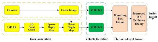
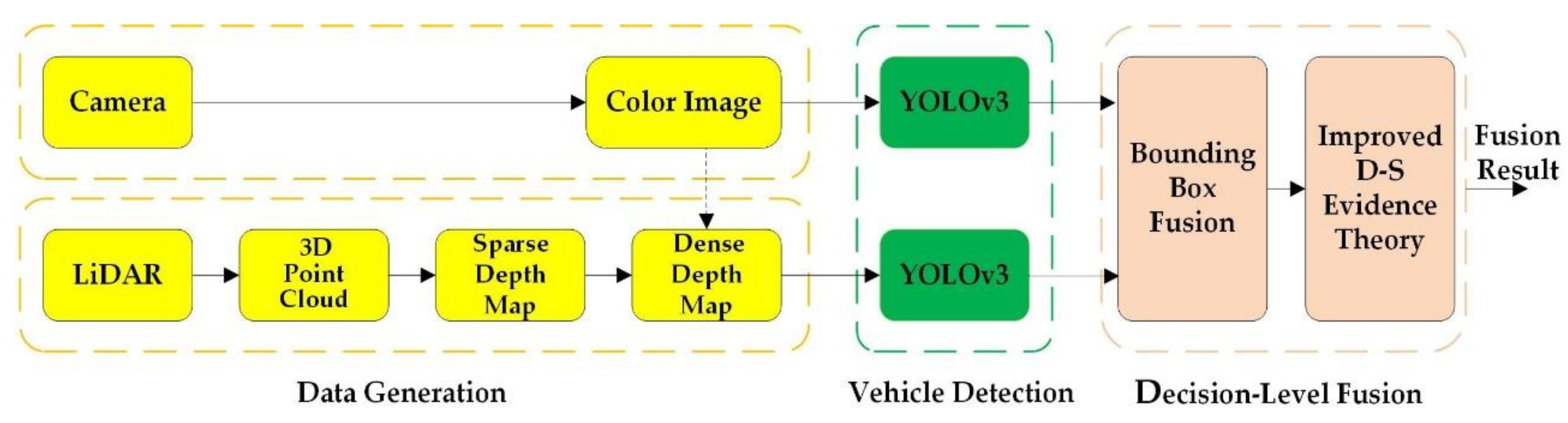
The framework consists of three parts, data generation, vehicle detection, and decision-level fusion. The overall structure of the framework is shown in Figure 1.

Figure 1. The structure of the framework.

First, the 3D LiDAR point cloud was transformed into a 2D sparse depth map by the joint calibration of camera and LiDAR, and then it was converted into a dense depth map by depth completion so that the laser data and image have the same resolution and are aligned with each other in space and time. Then the color image and dense depth map were input into the YOLOv3 detection network and the bounding box and confidence score of each detected vehicle were obtained. Finally, bounding box fusion and the improved Dempster–Shafer (D–S) evidence theory were proposed to obtain the final detection results.

2.1. Depth Completion

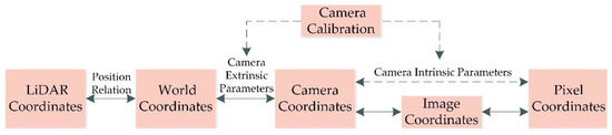
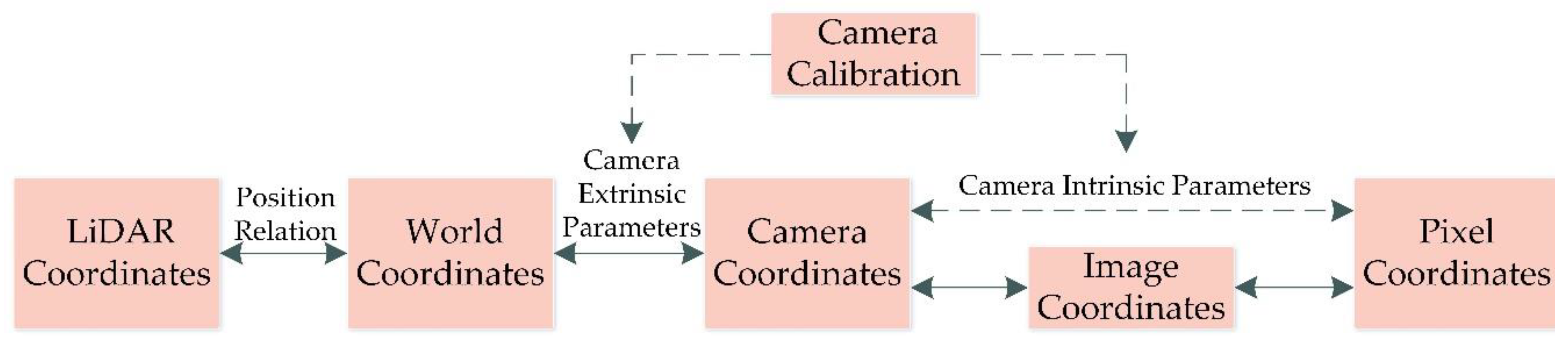
Before the depth completion, a pre-processing operation is required to convert the 3D LiDAR point cloud into a 2D sparse depth map. In pre-processing, the precise calibration, joint calibration, and synchronization of the LiDAR and camera are needed so that each 3D LiDAR point cloud can be projected accurately onto the 2D image plane to form the sparse depth map. The coordinate conversion relationship between the sensors is shown in Figure 2.

Figure 2. The coordinate conversion between the image and the light detection and ranging (LiDAR).

After the pre-processing work is completed, the sparse depth map is transformed into a dense depth map through the depth completion framework so that the resolution of LiDAR data and image is the same. The depth-completion method can be divided into two types, guided depth completion [22,26,27,28,29] and non-guided depth completion [21,30].

In the daytime, the camera can capture a clear, high-resolution image. Obviously, the image at this time is very useful for guiding depth completion because it can help to distinguish object boundaries and continuous smooth surfaces. However, at night, the sharpness of the image is greatly reduced. At this time, the image guidance will not help the result of the depth completion but will cause it to go in the wrong direction. Therefore, using only LiDAR data for depth completion will result in better outcomes. However, the commonly used depth completion methods have only a single completion mode, resulting in low image quality after completion. Low-quality images lose a lot of detailed features, which create difficulties for the later detection stages and will cause a large number of false detections and missed detections, which is not practical.

Therefore, this paper proposes a depth completion method that can switch between different completion modes according to day or night. Thus, this paper introduces the anisotropic diffusion tensor [31] and the proportionality coefficient, which can not only make the details of the dense depth map clearer but also switch between completion methods that require image guidance according to whether the image is clear or not.

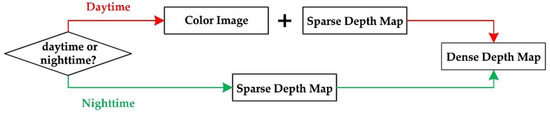
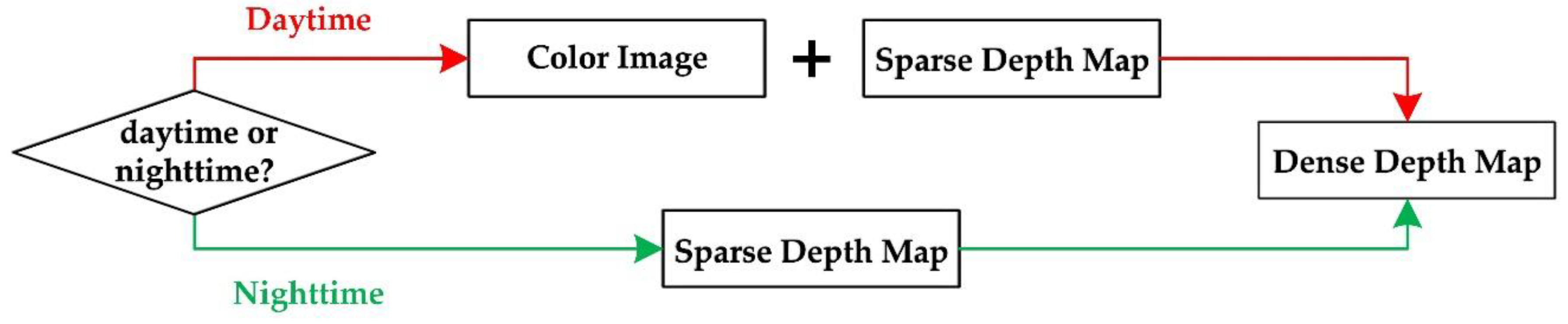
This method first judges whether the image is positively guiding the completion of the sparse depth map based on whether the acquired image is day or night. Here, there are many methods of day-night image classification, such as Bayesian classifier [32], SVM classifier, and CNN. When it is daytime, image-guided depth completion is used, and at night, only LiDAR data is used for completion. The specific flowchart is shown in Figure 3.

Figure 3. Depth completion flowchart.

Our completion method is mainly based on three hypotheses. One is that pixels with similar distances have similar depth values. The other is that similar color regions have similar depth values. The third is that changes in texture edges correspond to the mutation of depth values.

For all pixels with unknown depth, its depth value $D_p$ can be obtained using Equation (1):

$$D_p=\frac{1}{W_P}{\displaystyle \sum _{q\in \Omega }{D}_q{G}_{{\sigma }_D}(a\parallel p-q\parallel )G_{{\sigma }_I}(b\parallel I_p-I_q\parallel )G_{{\sigma }_T}(c\parallel T_p-T_q\parallel )}$$

(1)

$W_p$ is the normalization factor,

$$W_p={\displaystyle \sum _{q\in \Omega }{G}_{{\sigma }_D}(a\parallel p-q\parallel )G_{{\sigma }_I}(b\parallel I_p-I_q\parallel )G_{{\sigma }_T}(c\parallel T_p-T_q\parallel )}.$$

(2)

where p and q represent the position coordinates of the pixel, G represents the Gaussian function, I represents the pixel value of the image, D represents the depth value corresponding to the image, Ω represents the kernel of the Gaussian function and T represents anisotropic diffusion tensor.${\sigma }_I$, ${\sigma }_D$ and ${\sigma }_T$ are the $\sigma$ values of the Gaussian function of the color, distance, and anisotropic diffusion tensor, respectively. For the Gaussian function, the excessively large size of the convolution kernel results in fuzzy completion images. If the convolution kernel is set too small, the depth of unknown pixels around the sparse surroundings cannot be filled. In addition, the smoothness of the weight distribution depends on the size of σ. The larger the σ value, the smoother the weight distribution is. Therefore, after parameter tuning, the convolution kernel size is set between 5 and 15, when ${\sigma }_I={\sigma }_D={\sigma }_T=5~10$, and convolution kernel size is usually set to 9, σ is usually set to 7. The following details the anisotropic diffusion tensor and proportional coefficient.

(1) Anisotropic diffusion tensor

The anisotropic diffusion tensor is directly calculated from the color image, but it has a strong indication for the dense depth map formation because most texture edges correspond to depth value mutations. We use the anisotropic diffusion tensor to emphasize mutated regions of depth values and produce more accurate completion results.

Therefore, we include an anisotropic diffusion tensor T, which is calculated using the following equation:

$$T=\exp (-\beta {\left|\nabla I_H\right|}^{\gamma })n{n}^T+n^{\perp }{n}^{\perp T}$$

(3)

where $\nabla I_H$ is the image gradient and n is the normalized direction (unit vector) of the image gradient, $n=\nabla I_H/|\nabla I_H|$. $n^{\perp }$. is the normal vector of the image gradient. $\beta$ and γ can adjust the magnitude and sharpness of the tensor.

(2) Proportional coefficient

a, b and c are the proportional coefficients of distance variation, color variation, and anisotropic diffusion tensor variation, respectively. In the daytime, the value of the three coefficients can be adjusted to enlarge the details of the guide image so that the contour of the dense map is more evident. After parameter tuning, when $a=1,b=c=10~20$, the error of the dense depth map is the smallest, and the effect is the best, usually we set b and c are 15.

At night, we set a is 1, b and c are 0, the $G_{{\sigma }_I}\left(b\parallel I_P-I_p\parallel \right)G_{{\sigma }_T}\left(c\parallel T_p-T_q\parallel \right)$ value is constant. At this time, only the distance information is valid for the completion process. The entire equation is degraded to rely solely on LiDAR for depth completion, which enables switching between modes. However, if we only rely on the distance information for completion, the quality of the completion map is greatly affected, so we use the pre-processing operation of expansion and close operation to improve image sharpness.

2.2. Vehicle Detection

Because the YOLOv3 object detection model has not only breakneck detection speed but also excellent detection precision, this paper chooses YOLOv3 for vehicle detection. YOLOv3 is trained on two training sets (color image and dense depth map), and two trained models are finally obtained.

YOLO is a state-of-the-art real-time object detection model. YOLO has evolved through three iterations. YOLOv1 and YOLOv2 [33] are the first two-generation models of YOLO. They can process images at the rate of 45 frames per second (FPS), but they have the disadvantage of low detection precision. However, SSD, which belongs to the one-stage object detection model, not only has the same detection speed but also has better detection ability for small objects.

However, the emergence of YOLOv3 compensates for the imperfect detection ability of the previous two generations for small objects and maintains its speed advantage. YOLOv3 has a mean Average Precision (mAP) value of 57.9% on the COCO dataset, which is slightly higher than SSD and RetinaNet, but it is 2–4 times faster than them, 100 times faster than Fast R-CNN and 1000 times faster than R-CNN [24].

2.3. Decision-Level Fusion

In this section, based on the detection results of the dense depth map and the color image in YOLOv3, the obtained bounding box information and the corresponding confidence score are fused to obtain the final detection result.

2.3.1. Bounding Box Fusion

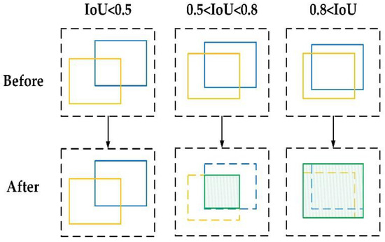
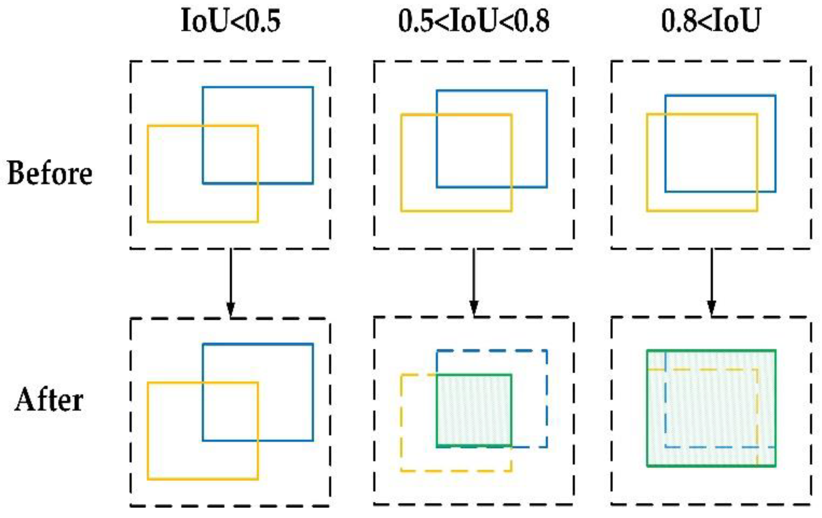
We choose different fusion strategies by judging the Intersection over Union (IoU) size of the bounding boxes in the dense depth map and color image. When IoU is less than 0.5, it is considered two independent detection objects without fusion. When IoU is between 0.5 and 0.8, and two bounding boxes have fewer overlaps, then the overlapping area is used as the final target area. When IoU is between 0.8 and 1, the two bounding boxes basically coincide. At this time, all the model boundaries are considered valid. We use the extended area of the bounding boxes as the new detection area. The effect is shown in Figure 4.

Figure 4. Bounding box fusion. The yellow area represents the bounding box detected by the dense depth map, and the blue area represents the bounding box detected by the color image, and the green area is the final detection result after fusion.

2.3.2. Confidence Score Fusion

For the fused bounding box, we take the corresponding confidence score of the original bounding box as a benchmark and obtain a new confidence score using improved D–S evidence theory.

D–S evidence theory is a no-exact reasoning theory introduced by Dempster and developed by Shafer. It is one of the most used methods for multi-sensor information fusion and is very suitable for decision-level fusion [34,35]. The specific flow of the algorithm is as follows:

Let $\mathsf{\Theta }$ be an identification framework, it is a set of mutually exclusive propositions, and the following formula holds:

$$m(\varnothing )=0,$$

(4)

$${\displaystyle \sum _{A\subseteq \theta }m(A)=1}.$$

(5)

$m{:2}^{\theta }\to \left[0,1\right]$, where $2^{\theta }$ is a set of all subsets of $\mathsf{\Theta }$ and $m\left(A\right)$ is the basic probability assignment (BPA) of A, also known as a mass function. The belief function (Bel) and the plausibility function (Pl) are defined as:

$$Bel(A)={\displaystyle \sum _{B\subseteq A}m(B),\forall A\subseteq \mathsf{\Theta }}$$

(6)

$$Pl(A)={\displaystyle \sum _{B\cap A\ne \varnothing }m(B)}$$

(7)

Suppose there are two evidences $E_1$ and $E_2$ under the identification framework $\mathsf{\Theta }$. The BPA and the focal elements of $E_1$ are $m_1$ and $A_1{,A}_2,\cdots {,A}_k$, respectively. The BPA and the focal elements of $E_2$ are $m_2$ and $B_1{,B}_2,\cdots {,B}_k$, respectively.

According to Dempster’s combination rule of Equation (8), the above evidence can be fused:

$$m(A)=m_1\oplus m_2=\{\begin{array}{ll}0& A=\varnothing \\ \frac{{\displaystyle \sum _{A_i\cap B_j=A}{m}_1(A_i)m_2(B_j)}}{1-k}& \forall A\subseteq \mathsf{\Theta },A\ne \varnothing \end{array}$$

(8)

where $k={\displaystyle \sum _{A_i\cap B_j=\varnothing }{m}_1(A_i)m_2(B_j)}$ reflects the degree of conflict of evidence.

But when Dempster’s combination rules are used to combine high-conflict evidence, it may lead to a wrong conclusion. At present, there are two ways to improve it. One is to modify the combination rules and the other is to modify the evidence before the improvement. Modifying the combination rule will destroy the excellent properties of the commutative law and the associative law of the Dempster rule. Therefore, this paper chooses to modify the evidence to solve this problem.

First, we introduce the distance between two evidences [36] to consider the degree of conflict between them. The distance between $m_1$ and $m_2$ is defined as follows:

$$d(m_1,m_2)=\sqrt{\frac{1}{2}{(\overrightarrow{m_1}-\overrightarrow{m_2})}^{T}D(\overrightarrow{m_1}-\overrightarrow{m_2})}.$$

(9)

where D is called the Jaccard coefficient and the size is a matrix of $2^{\theta }\times 2^{\theta }$, the value of each element is:

$$D(A,B)=\frac{|A\cap B|}{|A\cup B|} (A,B\in 2^{\theta }).$$

(10)

For n evidences, the distance matrix can be used to represent the distance between each two evidences:

$$D_{n\times n}=\left[\begin{array}{cccc}0& d(m_1,m_2)& \cdots & d(m_1,m_n)\\ d(m_2,m_1)& 0& \cdots & d(m_2,m_n)\\ ⋮& ⋮& ⋮& ⋮\\ d(m_n,m_1)& d(m_n,m_2)& \cdots & 0\end{array}\right]$$

(11)

The similarity $Sim$ [37] between the evidences can be obtained by the distance between the evidences, that is ${Sim(m}_i{,m}_j)=1-{d(m}_i{,m}_j)$, and the similarity matrix SM between the evidences is obtained by the same reasoning.

$$SM=\left[\begin{array}{cccc}1& Sim(m_1,m_2)& \cdots & Sim(m_1,m_n)\\ Sim(m_2,m_1)& 1& \cdots & Sim(m_2,m_n)\\ ⋮& ⋮& ⋮& ⋮\\ Sim(m_n,m_1)& Sim(m_n,m_2)& \cdots & 1\end{array}\right]$$

(12)

The degree of support for each evidence by other evidence can be defined as:

$$\mathrm{Crd}(m_i)={\displaystyle \sum _{\begin{array}{l}j=1\\ j\ne i\end{array}}^{n}Sim(m_i,m_j)}$$

(13)

Then the trust factor (weight) ${\omega }_i$ of the ith evidence $E_i$ can be obtained as:

$${\omega }_i=\frac{\mathrm{Crd}(m_i)}{{\displaystyle \sum _{i=1}^n\mathrm{Crd}(m_i)}}$$

(14)

After weighted averaging of the evidence, the expected evidence is obtained as:

$$M={\displaystyle \sum _{i=1}^n{\omega }_i}{m}_i$$

(15)

Finally, using D–S evidence theory, the result of n-1 iterative combinations of the expected evidence M are regarded as the synthesis result of n evidences.

3. Experimental Results and Discussion

We evaluated our method using the KITTI dataset [38] and the Waymo Open Dataset [39]. The KITTI dataset is the largest computer vision evaluation dataset for autonomous driving scenarios in the world. The data acquisition vehicle is equipped with a color camera and a Velodyne HDL-64E LiDAR. The Waymo Open Dataset is currently one of the largest and most diverse autonomous driving datasets in the world, with data from five LiDARs and five cameras. Our test platform is configured with an Intel Xeon E5-2670 CPU and an NVIDIA GeForce GTX 1080Ti GPU.

3.1. Depth Completion Experiment

The KITTI dataset provides calibration data for the camera and LiDAR, including rigid transformation matrix Tr_velo_to_cam from the LiDAR coordinate system to the camera coordinate system, camera internal parameter matrix P, and camera correction matrix R0_rect. Using Equation (16), we can project the LiDAR point cloud onto the camera plane to form a sparse depth map. In this process, points projected outside the image boundary need to be discarded. u and v are camera image coordinates, and x, y, z are 3D LiDAR coordinates.

$$\left[\begin{array}{l}u\\ v\\ 1\end{array}\right]=P•R0\_\mathrm{rect}•Tr\_\mathrm{velo}\_\mathrm{to}\_\mathrm{cam}•\left[\begin{array}{l}x\\ y\\ z\\ 1\end{array}\right]$$

(16)

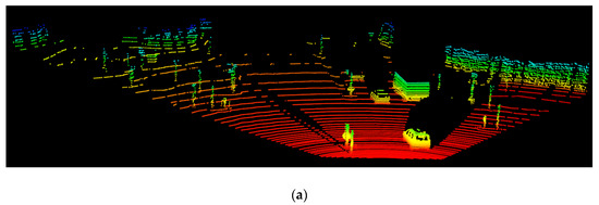
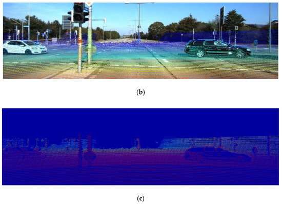
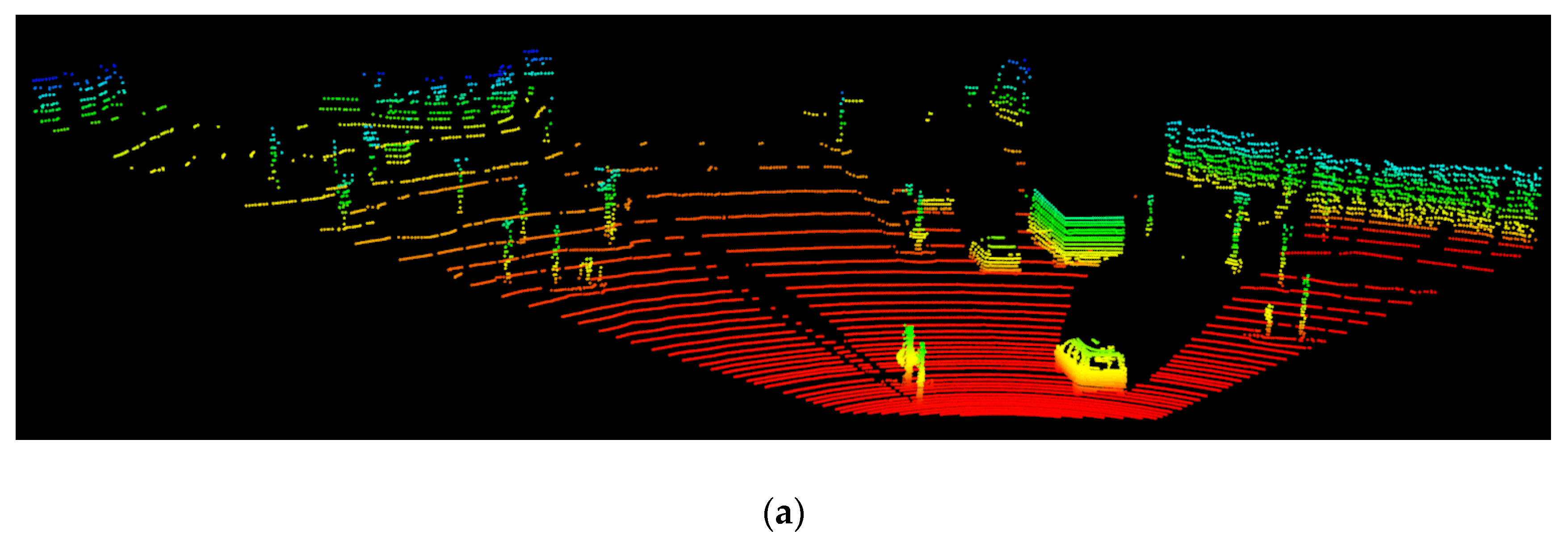
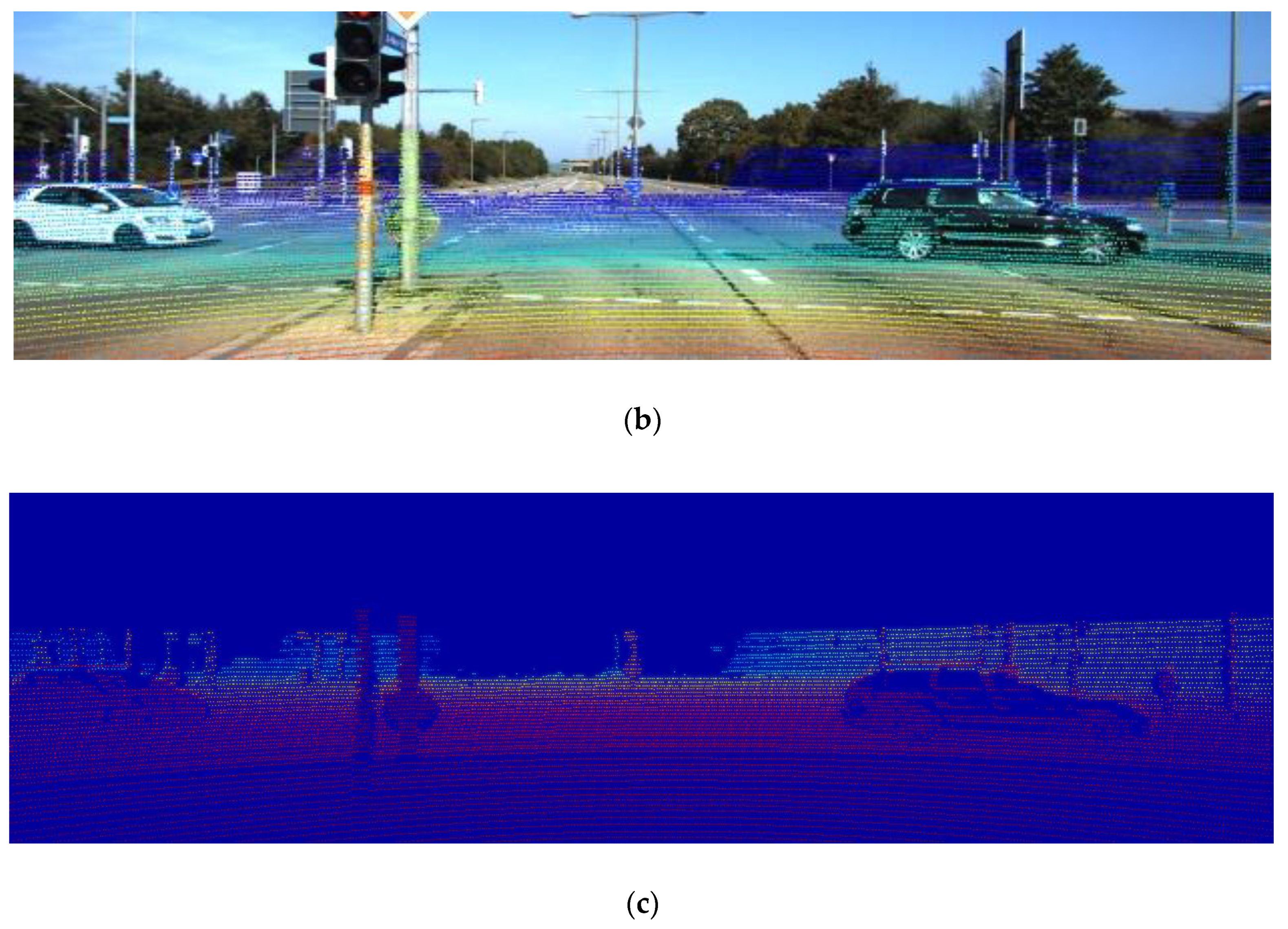
The conversion result of the sparse depth map is shown in Figure 5. In the fusion image, we can see that LiDAR points are well aligned with image pixels at the pillar. However the generated depth map is too sparse to obtain useful information directly.

Figure 5. The Conversion of 3D LiDAR point cloud to 2D sparse depth map. (a) 3D LiDAR point cloud image (only the areas that overlap with the image perspective are displayed, colored by height value); (b) fusion of image and LiDAR point cloud; (c) 2D sparse depth map (colored by depth).

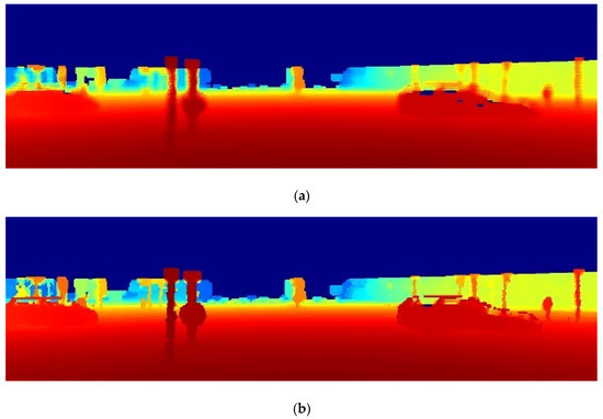
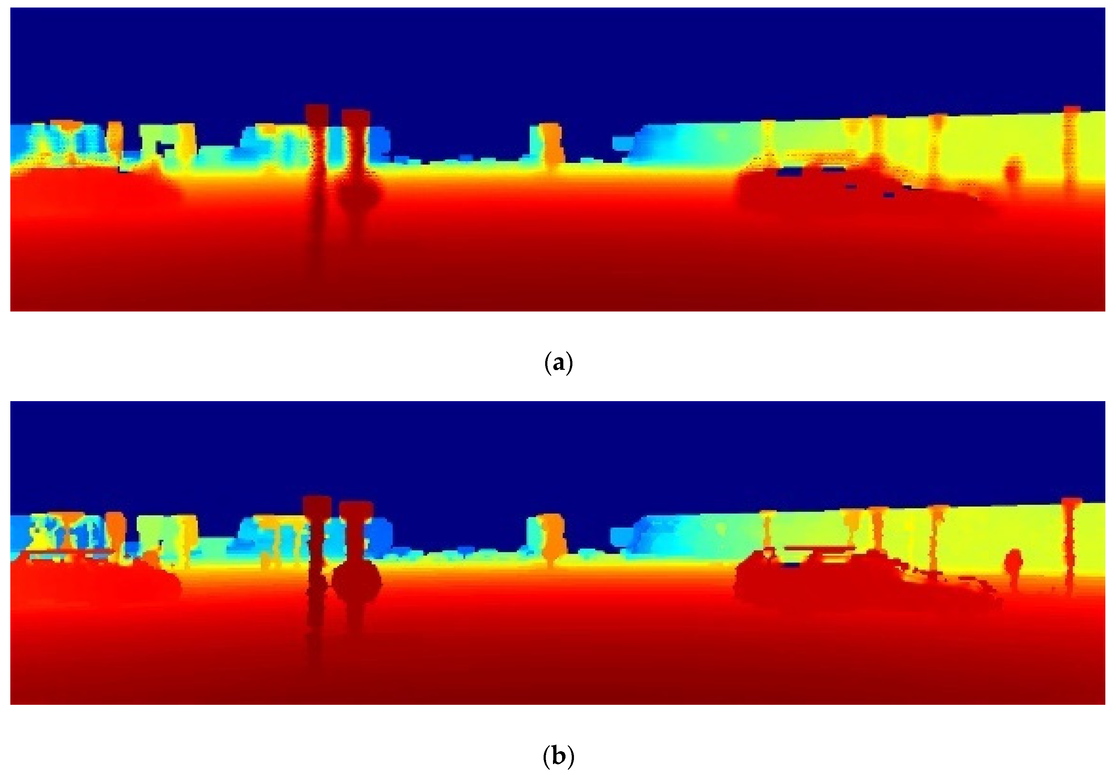
We undertook two kinds of processing of the LiDAR data at the same time and conducted experiments separately. When using only LiDAR data for completion, the results are shown in Figure 6. The contour edges of the image are more apparent after preprocessing.

Figure 6. Non-guided depth completion map. (a) Dense depth map without preprocessing; (b) dense depth map with preprocessing.

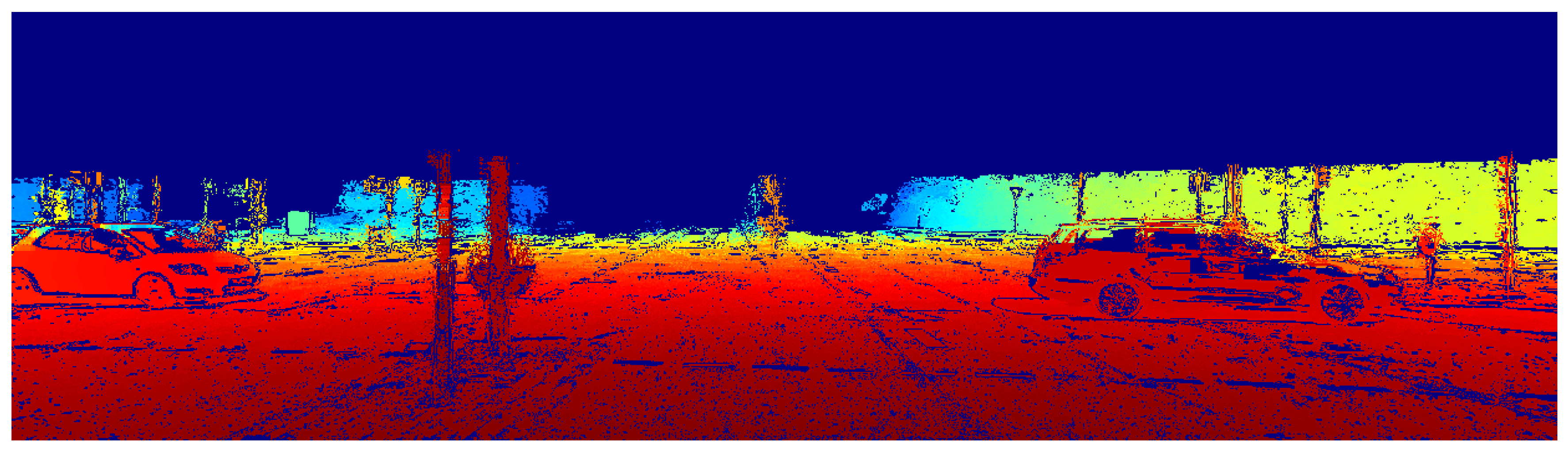
When the image is used for depth completion, the result is shown in Figure 7. The edge contour of the dense map is made more explicit by enlarging the edge information of the guide image. The basic outline of the vehicle can be seen clearly from the figure.

Figure 7. Guided depth completion map.

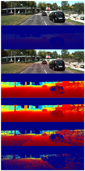
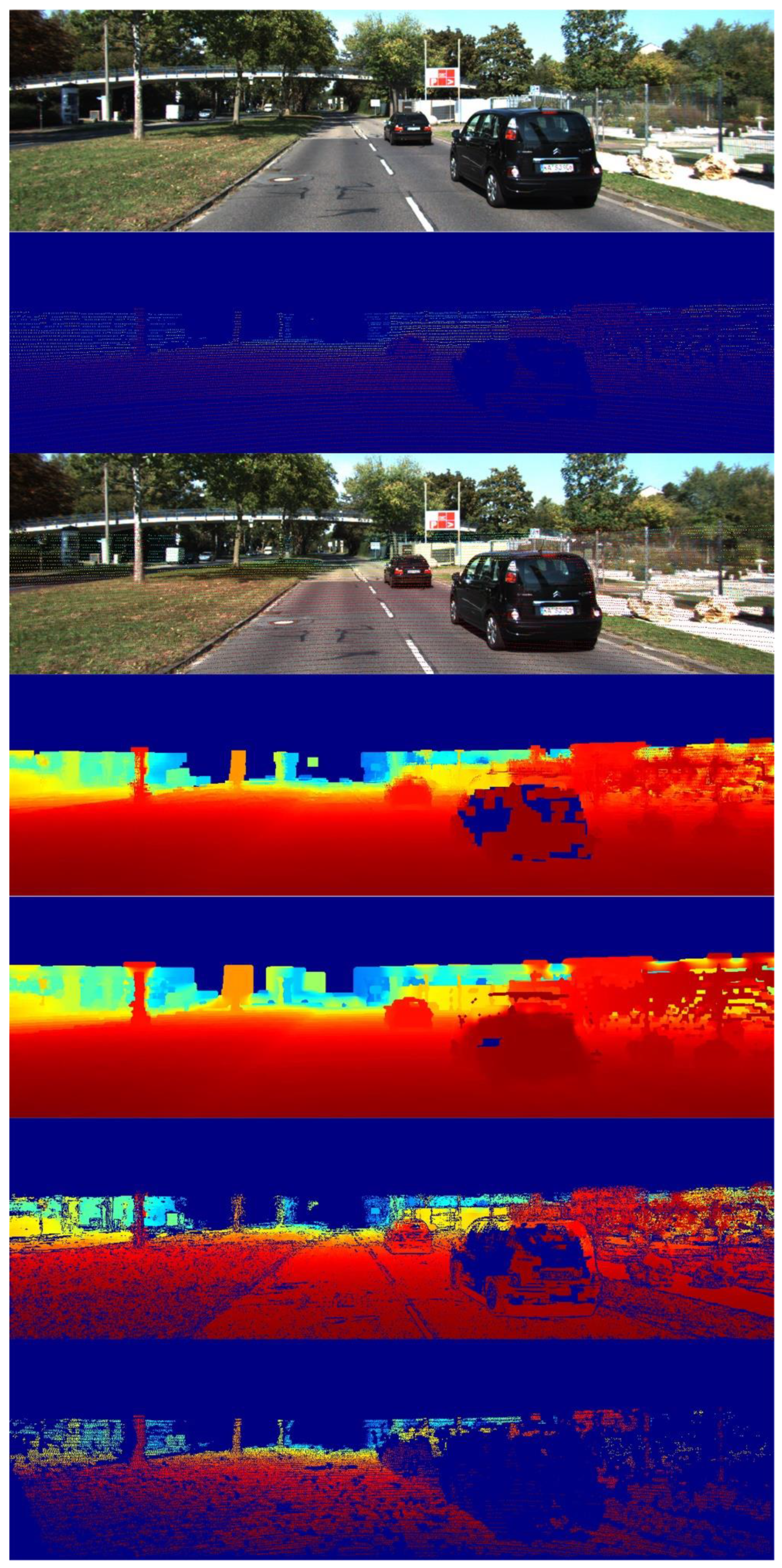
A full example of depth completion is shown in Figure 8. We visually compared our algorithm with the most commonly used joint bilateral upsampling (JBU) method and ground truth. It can be seen from the figure that depth completion significantly improves the resolution of LiDAR data and makes up for its low resolution. The completion map using the JBU method is blurred and the image quality is poor. In the non-guided depth completion map, the edges of objects are clear, and each object can be identified easily. The guided depth completion map is rich in detail, and the outline of the object in the map is clear and recognizable.

Figure 8. Comparison of depth completion methods. The images from top to bottom are the color image, sparse depth map, alignment effect map, dense depth map using JBU, Non-Guided depth completion map, Guided depth completion map, and ground truth.

To objectively evaluate the quality of the completion map, we introduce the root mean square error (RMSE), mean absolute error (MAE), inverse root mean square error (iRMSE) and inverse mean absolute error (iMAE):

$$RMSE=\sqrt{\frac{{\displaystyle \sum _{m=1}^M{\displaystyle \sum _{n=1}^N{[R(m,n)-I(m,n)]}^2}}}{MN}}$$

(17)

$$MAE=\frac{1}{MN}{\displaystyle \sum _{m=1}^M{\displaystyle \sum _{n=1}^N|R(m,n)-I(m,n)|}}$$

(18)

$$iRMSE=\sqrt{\frac{{\displaystyle \sum _{m=1}^M{\displaystyle \sum _{n=1}^N{[\frac{1}{R(m,n)}-\frac{1}{I(m,n)}]}^2}}}{MN}}$$

(19)

$$iMAE=\frac{1}{MN}{\displaystyle \sum _{m=1}^M{\displaystyle \sum _{n=1}^N|\frac{1}{R(m,n)}-\frac{1}{I(m,n)}|}}$$

(20)

where R(m, n) and I(m, n) represent the reference image and the target image, respectively. The reference image has true depth value, and M and N represent the size of the image.

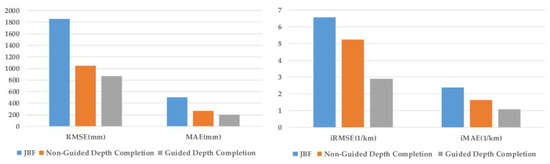
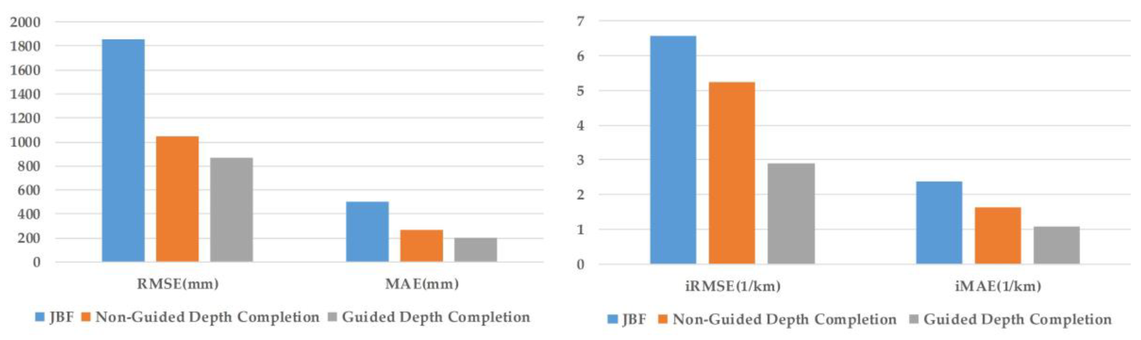
We experimented with 1000 groups of data with ground truth in the KITTI depth completion dataset and averaged all the errors. The results are shown in Table 1 and Figure 9. It is evident that our proposed method has a minimal error.

Table 1. Error comparison of completion results.

Method	RMSE (mm)	MAE (mm)	iRMSE (1/km)	iMAE (1/km)
Joint bilateral upsampling (JBU)	1856.83	501.64	6.58	2.38
Non-guided depth completion	1046.21	266.50	5.23	1.63
Guided depth completion	865.62	200.7	2.91	1.09

Figure 9. Error comparison of completion results.

3.2. Vehicle Detection and Fusion Experiment

The KITTI object detection dataset contains 7481 frames of training data and 7518 frames of test data. Each frame contains a synchronized color image and LiDAR datapoint. There are nine classes of label information in the dataset, including ‘Car’, ‘Van’, ‘Truck’, ‘Pedestrian’, ‘Person sitting’, ‘Cyclist’, ‘Tram’, ‘Misc’, and ‘Don’t Care’. We merged the classes ‘Car’, ‘Van’, ‘Tram’, and ‘Truck’ into the new class ‘vehicle’, and only detected vehicles. Since the ground truth of the testing set has not yet been released. We divided 7481 frames of the training set randomly into two parts, 3741 framed for training and 3740 frames for testing.

Since the KITTI dataset only has daytime driving data, to test the night driving data, this paper further introduces the Waymo Open Dataset, which contains high-resolution images and LiDAR data of 1000 fragments under various conditions. We validated the method using its 64-layer mid-range LiDAR data and the images of the front camera in its night environment. We trained color image, guided depth completion map (daytime), and non-guided depth completion map (nighttime) in YOLOv3, and fused the results of the color image and depth completion map. Mini-batch gradient descent (MBGD) is used to optimize our network. We trained network for about 180 epochs. Throughout the training process, the network with $1242\times 375$ input was trained with a batch size of 8. The initial value of leaning rate was ${10}^{-3}$, which changed to ${10}^{-4}$ after 100 epochs, and ${10}^{-5}$ after 40 epochs. The momentum and weight decay were configured as 0.9 and 0.0005.

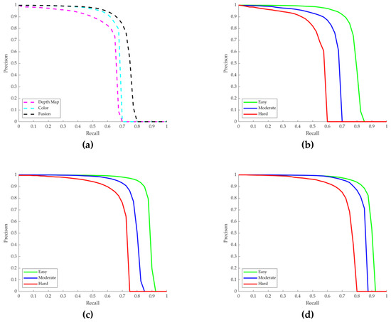
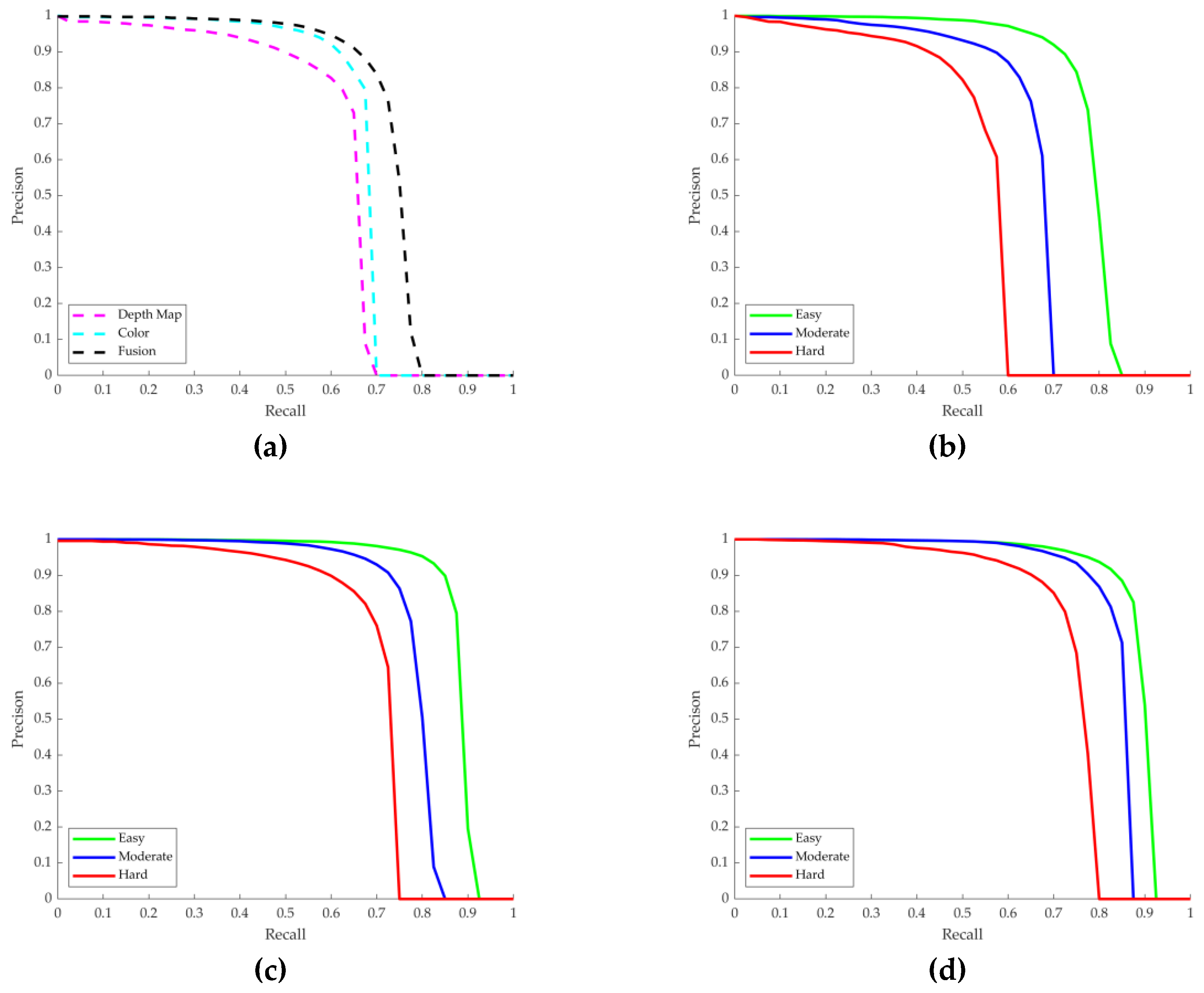
We were consistent with the evaluation method of the KITTI dataset, using average precision (AP) and IoU [40] to evaluate the detection performance. When the IoU overlap threshold was greater than 0.7, the detection was considered successful. According to the size of bounding box height, occlusion level, and truncation, the KITTI dataset is divided into three different levels, easy, moderate, and hard. Figure 10 shows the precision-recall (P-R) curves for day detection, night detection, and the fusion result. Table 2 shows the AP of the day detection results, and Table 3 shows the AP of the night detection results.

Figure 10. Precision-recall (P-R) curve. (a) Night experiment results; (b) dense depth map detection results in the daytime; (c) color image detection results in the daytime; (d) daytime fusion results.

Table 2. Performance evaluation of every detector during the day.

Method	Easy	Moderate	Hard
Guided Depth Completion	75.13%	62.34%	51.26%
color	82.17%	77.53%	68.47%
Fusion	85.62%	80.16%	70.19%

Table 3. Performance evaluation of each detector at night.

	Color	Non-Guided Depth Completion	Fusion
AP	65.47%	60.13%	69.02%

As can be seen from the chart, both day and night, dense depth maps and color images can get excellent detection precision, and after fusion, the precision is improved. Compared with the results of daytime image detection, the results of daytime fusion detection are 3.45, 2.63, and 1.72% higher in easy, moderate, and hard, respectively. Compared with the results of night image detection, the results of night fusion detection increased AP by 3.55%.

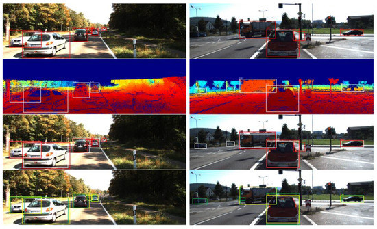
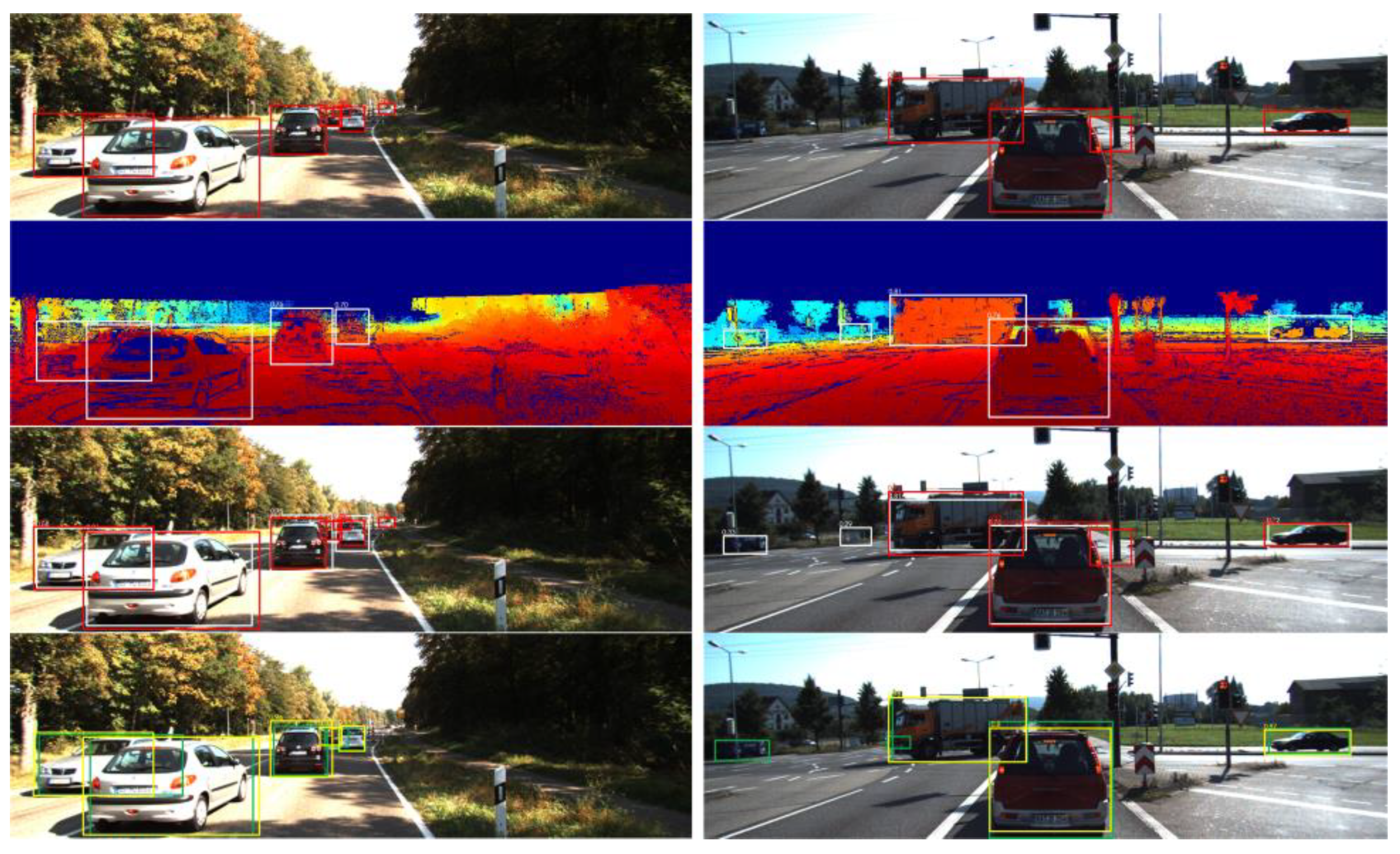
An example of the fusion detection process is shown in Figure 11, Figure 12, Figure 13 and Figure 14. Good detection results can be obtained by color image and dense depth image alone. After fusion, the detection advantages of both are considered comprehensively; more accurate results are obtained.

Figure 11. Fusion detection process. The images from top to bottom are: detection results of color images (red), detection results of dense depth maps (white), fusion process of the former two, fusion results (yellow), and ground truth(green).

Figure 12. Distance calculation area selection. The shadow area is not involved in the calculation.

Figure 13. Final test results.

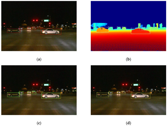
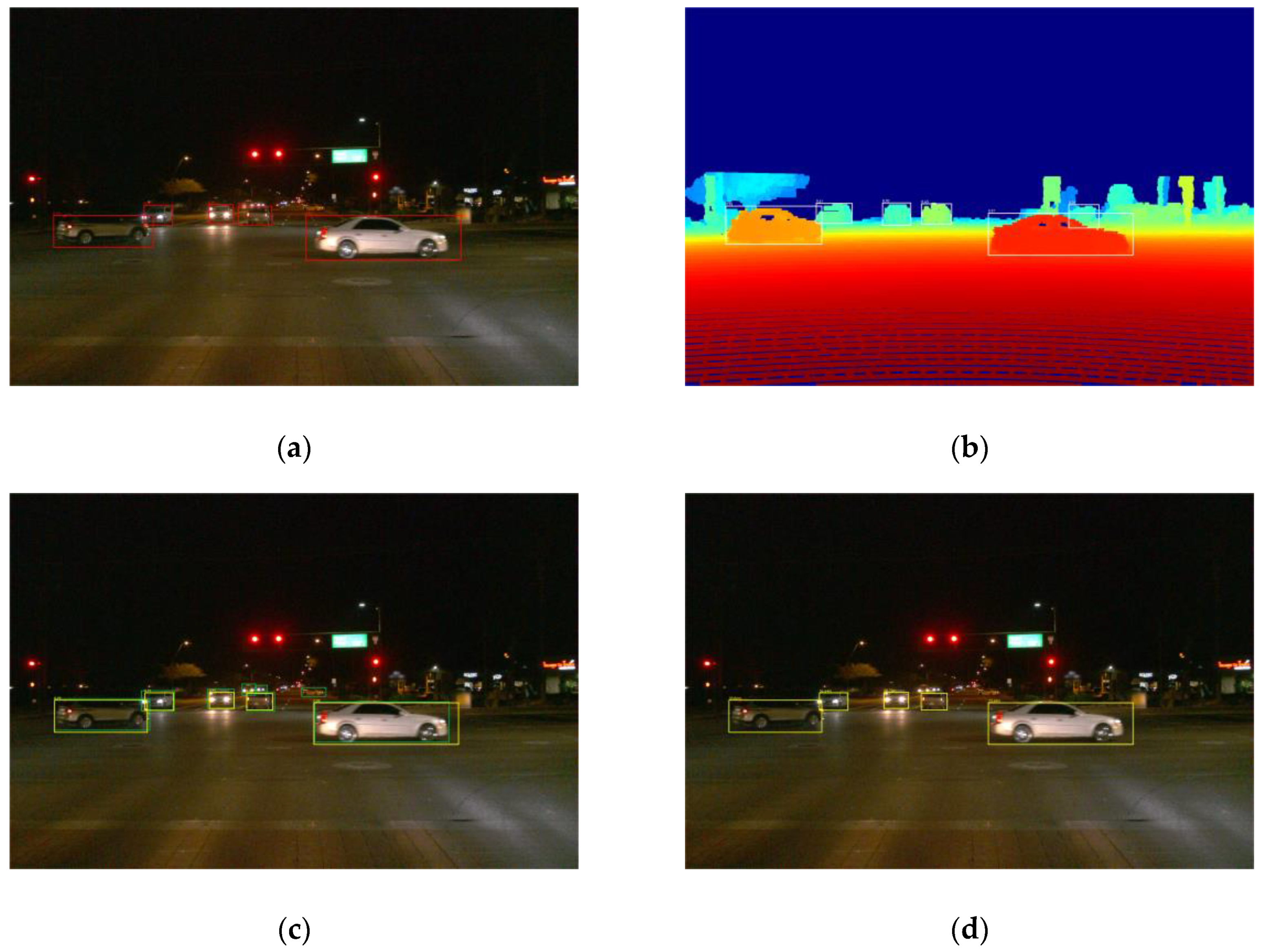
Figure 14. Detection process at night. (a) detection results of color images (red); (b) detection results of dense depth maps (white); (c) fusion results (yellow) and ground truth(green); (d) distance detection results.

The distance information of the vehicle can be obtained through the final bounding box and the dense depth map. We first removed the overlapped area between the bounding boxes to filter out other vehicle information. An example is shown in Figure 12.

However, the remaining bounding box still contains some background information and invalid points. Therefore, we should first remove the invalid points with a depth value of 0. Then we should remove the points with a maximum depth value of 30% and a minimum depth value of 10% of the remaining part, and average the depth value of the final remaining part to get the distance from LiDAR to the preceding vehicle. Then, we subtract the distance between LiDAR and the vehicle front-body by 2.89 m to obtain the final vehicle distance. Figure 13 shows the final calculation results.

Similarly, an example of the night detection process is shown in Figure 14. The detection result is more accurate after fusion and the distance information of the vehicle is obtained.

To further evaluate the effectiveness of the proposed algorithm, we compared our method with state-of-the-art object detection methods. The results are shown in Table 4.

Table 4. Comparisons to previously published results.

Method	KITTI			Waymo	Time	Environment
	Easy	Moderate	Hard	Night
Faster R-CNN [4]	87.90%	79.11%	70.19%	68.37%	2s	GPU@3.5Ghz
MV3D [18]	89.80%	79.76%	78.61%	/	0.24s	GPU@2.5Ghz
3DVP	81.46%	75.77%	65.38%	63.84%	40s	GPU@3.5Ghz
3DOP [7]	90.09%	88.34%	78.39%	77.42%	3s	GPU@2.5Ghz
MS-CNN [5]	90.03%	89.02%	76.11%	73.57%	0.4s	GPU@2.5Ghz
Yolov2 [32]	74.35%	62.65%	53.23%	56.45%	0.03s	GPU@3.5Ghz
Yolov3 [24]	82.17%	77.53%	68.47%	65.47%	0.04s	GPU@2.5Ghz
R-SSD [41]	88.13%	82.37%	71.73%	/	0.08s	GPU@2.5Ghz
SubCat	81.45%	75.46%	59.71%	/	0.7s	GPU@3.5Ghz
Mono3D [8]	90.27%	87.86%	78.09%	77.51%	4.2s	GPU@2.5Ghz
SubCNN [6]	90.75%	88.86%	79.24%	/	2s	GPU@3.5Ghz
Fusion	85.62%	80.46%	70.19%	69.02%	0.057s	GPU@2.5Ghz

For daytime detection, in terms of precision, ranking with moderate difficulty, our method ranks fifth out of 10 methods, and it has reached a high detection precision and fully meets the requirements of practical application.

In terms of speed, our method has a breakneck detection speed of 0.057 s, only 0.027 s slower than YOLOv2, but the average AP is 15.35% higher. Compared with Faster R-CNN with similar AP, our method is 35 times faster. Compared with R-SSD with similar performance, our method has a stronger anti-interference ability. Compared with MS-CNN, SubCNN, 3DOP, and Mono3D methods with high AP, our method is 7×, 35×, 53×, and 73× faster, respectively.

For nighttime detection, the method in this paper still has excellent performance, ranking third in detection precision and third in detection speed among all the compared methods.

In conclusion, compared with other models, our method achieves advanced detection precision, has fast detection speed, and has a strong anti-jamming ability, so it is fully capable of autonomous vehicle detection tasks.

4. Conclusions

This paper proposes a multi-adaptive real-time decision-level fusion framework combining LiDAR and camera. The framework consists of three parts, multi-adaptive completion, real-time detection, and decision-level fusion. The three parts are complementary. First, a multi-adaptive high-precision depth completion method is proposed, which improves the quality of the dense depth map. Then, we chose the YOLOv3 object detection model to ensure real-time performance. Finally, the bounding box fusion method and improved D–S evidence theory were designed to fit the application environment of this framework better. These decision-level fusion methods combine the detection results of the two sensors to achieve complementary advantages.

The experimental results show that the depth completion algorithm proposed in this paper is beneficial for vehicle detection, and the average detection accuracy is improved by 2.84% through the decision-level fusion scheme. The processing time of each frame of data only needs 0.057s, which is much shorter than the response time of 0.2s for human drivers, and fully meets the real-time requirements.

Although our depth completion algorithm is designed for vehicle detection, it can also be applied to popular research fields such as Simultaneous Localization and Mapping(SLAM), 3D object detection, and optical flow. The proposed decision-level fusion method is also universal in the field of sensor fusion.

References

- Ross, G.; Jeff, D.; Trevor, D.; Jitendra, M. Rich Feature Hierarchies for Accurate Object Detection and Semantic Segmentation. In Proceedings of the IEEE Conference on Computer Vision and Pattern Recognition (CVPR), Columbus, OH, USA, 24–27 June 2014; pp. 580–587. [Google Scholar]
- He, K.; Zhang, X.; Ren, S.; Sun, J. Spatial pyramid pooling in deep convolutional networks for visual recognition. IEEE Trans. Pattern Anal. Mach. Intell. 2015, 37, 1904–1916. [Google Scholar] [CrossRef] [Scilit] [PubMed]
- Ross, G. Fast R-CNN. In Proceedings of the 2015 IEEE International Conference on Computer Vision (ICCV), Santiago, Chile, 7–13 December 2015; pp. 1440–1448. [Google Scholar]
- Ren, S.; He, K.; Girshick, R.; Sun, J. Faster R-CNN: Towards Real-Time Object Detection with Region Proposal Networks. IEEE Trans Patt. Anal. Mach. Intell. 2017, 39, 1137–1149. [Google Scholar] [CrossRef] [Scilit] [PubMed]
- Cai, Z.; Fan, Q.; Feris, R.S.; Vasconcelos, N. A unified multi-scale deep convolutional neural network for fast object detection. In Proceedings of the EUropean Conference on Computer Vision, Amsterdam, The Netherlands, 8–16 October 2016; pp. 354–370. [Google Scholar]
- Xiang, Y.; Choi, W.; Lin, Y.; Savarese, S. Subcategory-aware convolutional neural networks for object detection. In Proceedings of the IEEE Winter Conference on Applications Computer Vision (WACV), Santa Rosa, CA, USA, 27–29 March 2017; pp. 924–933. [Google Scholar]
- Chen, X.; Kundu, K.; Zhu, Y.; Berneshawi, A.; Ma, H.; Fidler, S.; Urtasun, R. 3D Object Proposals for Accurate Object Class Detection. In Proceedings of the 29th Annual Conference on Neural Information Processing Systems (NIPS), Montreal, QC, Canada, 7–12 December 2015; pp. 424–432. [Google Scholar]
- Chen, X.; Kundu, K.; Zhang, Z.; Ma, H.; Fidler, S.; Urtasun, R. Monocular 3d Object Detection for Autonomous Driving. In Proceedings of the IEEE Conference on Computer Vision and Pattern Recognition (CVPR), Las Vegas, NV, USA, 26 June–1 July 2016; pp. 2147–2156. [Google Scholar]
- Liu, W.; Anguelov, D.; Erhan, D.; Szegedy, C.; Reed, S.; Fu, C.Y.; Berg, A.C. SSD: Single Shot MultiBox Detector. In Proceedings of the 14th European Conference ECCV 2016, Amsterdam, The Netherlands, 11–14 October 2016; pp. 21–37. [Google Scholar]
- Lin, T.-Y.; Goyal, P.; Girshick, R.; He, K.; Dollar, P. Focal Loss for Dense Object Detection. In Proceedings of the IEEE International Conference on Computer Vision, Venice, Italy, 22–29 October 2017; pp. 2999–3007. [Google Scholar]
- Redmon, J.; Divvala, S.; Girshick, R.; Farhadi, A. You only look once: Unified, real-time object detection. In Proceedings of the IEEE Conference on Computer Vision and Pattern Recognition, Las Vegas, NV, USA, 27–30 June 2016; pp. 779–788. [Google Scholar]
- Zhou, Y.; Tuzel, O. VoxelNet: End-to-End Learning for Point Cloud Based 3D Object Detection. In Proceedings of the IEEE Conference on Computer Vision and Pattern Recognition (CVPR), Salt Lake City, UT, USA, 18–22 June 2018; pp. 4490–4499. [Google Scholar]
- Asvadi, A.; Premebida, C.; Peixoto, P.; Nunes, U. 3D Lidar-based static and moving obstacle detection in driving environments: An approach based on voxels and multi-region ground planes. Robot. Auton. Syst. 2016, 83, 299–311. [Google Scholar] [CrossRef] [Scilit]
- Sualeh, M.; Kim, G.W. Dynamic multi-lidar based multiple object detection and tracking. Sensors 2019, 19, 1474. [Google Scholar] [CrossRef] [Scilit]
- Brummelen, J.V.; O’Brien, M. Autonomous vehicle perception: The technology of today and tomorrow. Transp. Res. C. 2018, 89, 384–406. [Google Scholar] [CrossRef] [Scilit]
- Garcia, F.; Martin, D.; De La Escalera, A.; Armingol, J.M. Sensor fusion methodology for vehicle detection. IEEE Intell. Transp. Syst. Mag. 2017, 9, 123–133. [Google Scholar] [CrossRef] [Scilit]
- Gao, H.; Cheng, B.; Wang, J.; Li, K.; Zhao, J.; Li, D. Object classification using cnn-based fusion of vision and lidar in autonomous vehicle environment. IEEE Trans. Ind. Inf. 2018, 14, 4224–4231. [Google Scholar] [CrossRef] [Scilit]
- Chen, X.; Ma, H.; Wan, J.; Li, B.; Xia, T. Multi-view 3D Object Detection Network for Autonomous Driving. In Proceedings of the 2017 IEEE Conference on Computer Vision and Pattern Recognition (CVPR), Honolulu, HI, USA, 21–26 July 2017. [Google Scholar]
- Matti, D.; Ekenel, H.K.; Thiran, J.-P. Combining LiDAR Space Clustering and Convolutional Neural Networks for Pedestrian Detection. In Proceedings of the 14th IEEE International Conference on Advanced Video and Signal Based Surveillance (AVSS), Lecce, Italy, 29 August–1 September 2017. [Google Scholar]
- Wang, H.; Lou, X.; Cai, Y.; Li, Y.; Chen, L. Real-Time Vehicle Detection Algorithm Based on Vision and Lidar Point Cloud Fusion. J. Sens. 2019, 2019, 8473980. [Google Scholar] [CrossRef] [Scilit]
- De Silva, V.; Roche, J.; Kondoz, A. Robust fusion of LiDAR and wide-angle camera data for autonomous mobile robots. Sensors 2018, 18, 2730. [Google Scholar] [CrossRef] [Scilit]
- Premebida, C.; Carreira, J.; Batista, J.; Nunes, U. Pedestrian detection combining RGB and dense LIDAR data. In Proceedings of the IEEE/RSJ International Conference on Intelligent Robots and Systems, Chicago, IL, USA, 14–18 September 2014; pp. 4112–4117. [Google Scholar]
- Oh, S.I.; Kang, H.B. Object Detection and Classification by Decision-Level Fusion for Intelligent Vehicle Systems. Sensors 2017, 17, 207. [Google Scholar] [CrossRef] [Scilit]
- Chavez-Garcia, R.O.; Aycard, O. Multiple sensor fusion and classification for moving object detection and tracking. IEEE Trans. Intell. Transp. Syst. 2016, 17, 525–534. [Google Scholar] [CrossRef] [Scilit]
- Redmon, J.; Farhadi, A. YOLOv3: An Incremental Improvement. arXiv 2018, arXiv:1804.02767. [Google Scholar]
- Liu, W.; Jia, S.; Li, P.; Chen, X. An MRF-Based Depth Upsampling: Upsample the Depth Map With Its Own Property. IEEE Signal Process. Lett. 2015, 22, 1708–1712. [Google Scholar] [CrossRef] [Scilit]
- Kopf, J.; Cohen, M.F.; Lischinski, D.; Uyttendaele, M. Joint bilateral upsampling. Acm Trans. Graph. 2007, 26, 96. [Google Scholar] [CrossRef]
- Yang, Q.; Yang, R.; Davis, J.; Nistér, D. Spatial-Depth Super Resolution for Range Images. In Proceedings of the 2007 IEEE Computer Society Conference on Computer Vision and Pattern Recognition (CVPR), Minneapolis, MN, USA, 18–23 June 2007; pp. 1–8. [Google Scholar]
- Premebida, C.; Garrote, L.; Asvadi, A.; Ribeiro, P.; Nunes, U. High-resolution LIDAR-based Depth Mapping using Bilateral Filter. In Proceedings of the IEEE international conference on intelligent transportation systems (ITSC), Rio de Janeiro, Brazil, 1–4 November 2016; pp. 2469–2474. [Google Scholar]
- Ashraf, I.; Hur, S.; Park, Y. An Investigation of Interpolation Techniques to Generate 2D Intensity Image From LIDAR Data. IEEE Access 2017, 5, 8250–8260. [Google Scholar] [CrossRef] [Scilit]
- Ferstl, D.; Reinbacher, C.; Ranftl, R.; Ruether, M.; Bischof, H. Image guided depth upsampling using anisotropic total generalized variation. In Proceedings of the IEEE International Conference on Computer Vision (ICCV), Sydney, Australia, 1–8 December 2013; pp. 993–1000. [Google Scholar]
- Hsieh, H.Y.; Chen, N. Recognising daytime and nighttime driving images using Bayes classifier. IET Intell. Transp. Syst. 2012, 6, 482–493. [Google Scholar] [CrossRef] [Scilit]
- Redmon, J.; Farhadi, A. YOLO9000: Better, faster, stronger. arXiv 2016, arXiv:1612.08242. [Google Scholar]
- Tang, H.; Su, Y.; Wang, J. Evidence theory and differential evolution based uncertainty quantification for buckling load of semi-rigid jointed frames. Sadhana 2015, 40, 1611–1627. [Google Scholar] [CrossRef] [Scilit]
- Wang, J.; Liu, F. Temporal evidence combination method for multi-sensor target recognition based on DS theory and IFS. J. Syst. Eng. Electron. 2017, 28, 1114–1125. [Google Scholar]
- Jousselme, A.-L.; Grenier, D.; Bossé, É. A new distance between two bodies of evidence. Inf. Fusion 2001, 2, 91–101. [Google Scholar] [CrossRef] [Scilit]
- Han, D.; Deng, Y.; Liu, Q. Combining belief functions based on distance of evidence. Decis. Support Syst. 2005, 38, 489–493. [Google Scholar]
- Geiger, A.; Lenz, P.; Urtasun, R. Are we ready for autonomous driving? The KITTI vision benchmark suite. In Proceedings of the 2012 IEEE Conference on CVPR, Providence, RI, USA, 16–21 June 2012; pp. 3354–3361. [Google Scholar]
- Sun, P.; Kretzschmar, H.; Dotiwalla, X.; Chouard, A.; Patnaik, V.; Tsui, P.; Guo, J.; Zhou, Y.; Chai, Y.; Caine, B.; et al. Scalability in Perception for Autonomous Driving: Waymo Open Dataset. arXiv 2019, arXiv:1912.04838. [Google Scholar]
- Everingham, M.; Van Gool, L.; Williams, C.K.; Winn, J.; Zisserman, A. The pascal visual object classes (voc) challenge. Int. J. Comput. Vis. 2010, 88, 303–338. [Google Scholar] [CrossRef] [Scilit]
- Jeong, J.; Park, H.; Kwak, N. Enhancement of SSD by concatenating feature maps for object detection. arXiv 2017, arXiv:1705.09587v1. [Google Scholar]
© 2020 by the authors. Licensee MDPI, Basel, Switzerland. This article is an open access article distributed under the terms and conditions of the Creative Commons Attribution (CC BY) license (http://creativecommons.org/licenses/by/4.0/).