Real-Time Vehicle Detection Framework Based on the Fusion of LiDAR and Camera


Abstract
1. Introduction
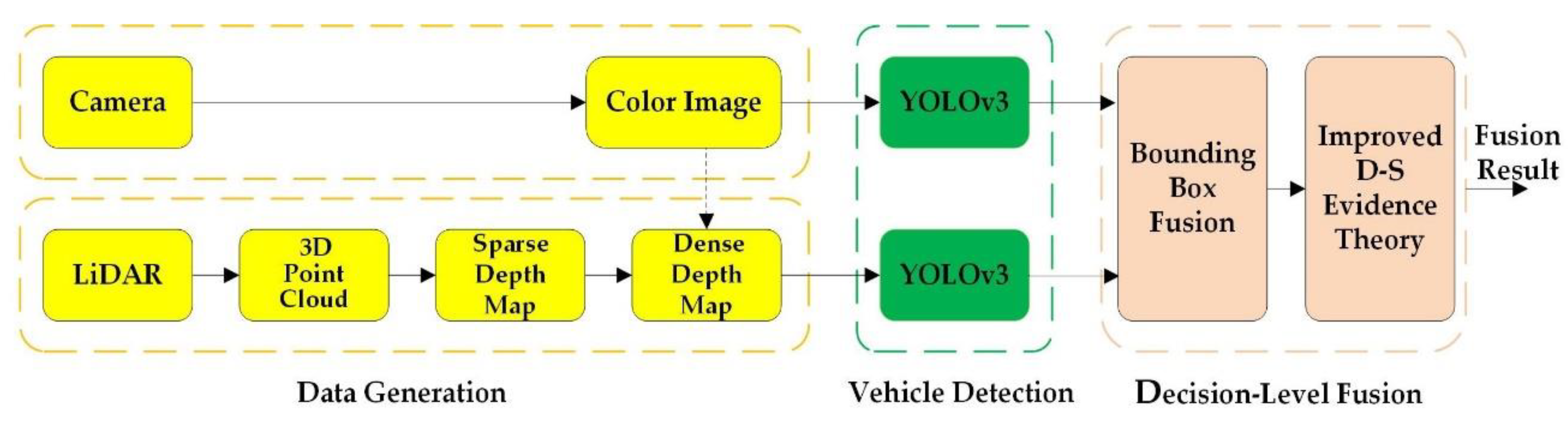
2. Methodology
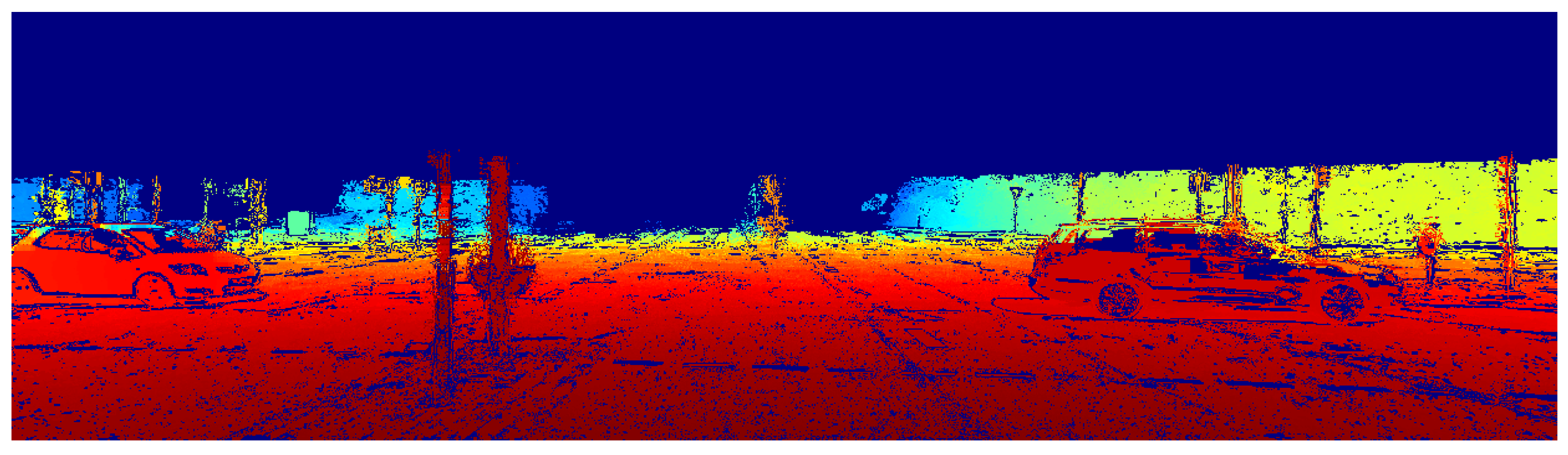
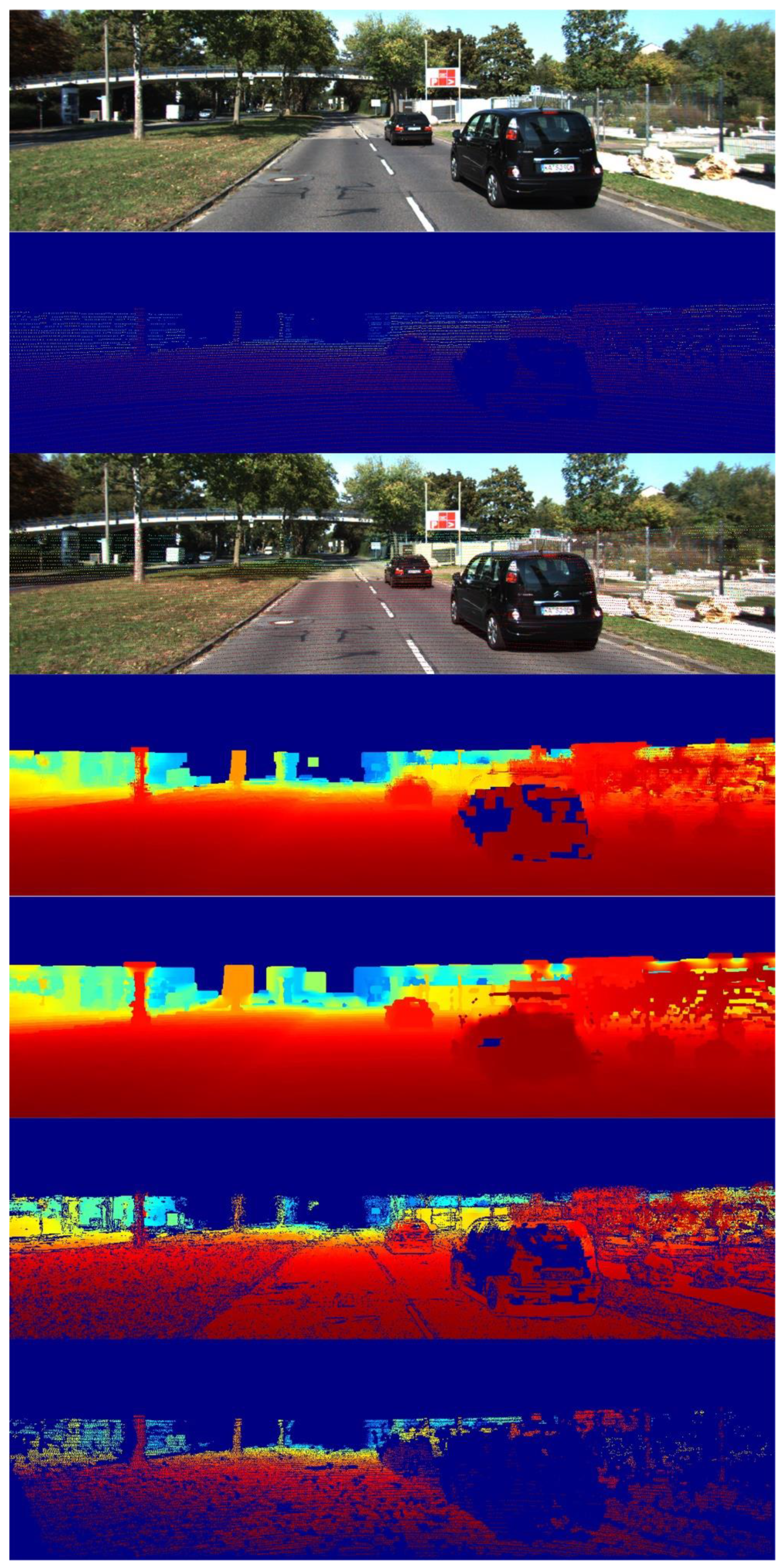
2.1. Depth Completion
2.2. Vehicle Detection
2.3. Decision-Level Fusion
2.3.1. Bounding Box Fusion
2.3.2. Confidence Score Fusion
3. Experimental Results and Discussion
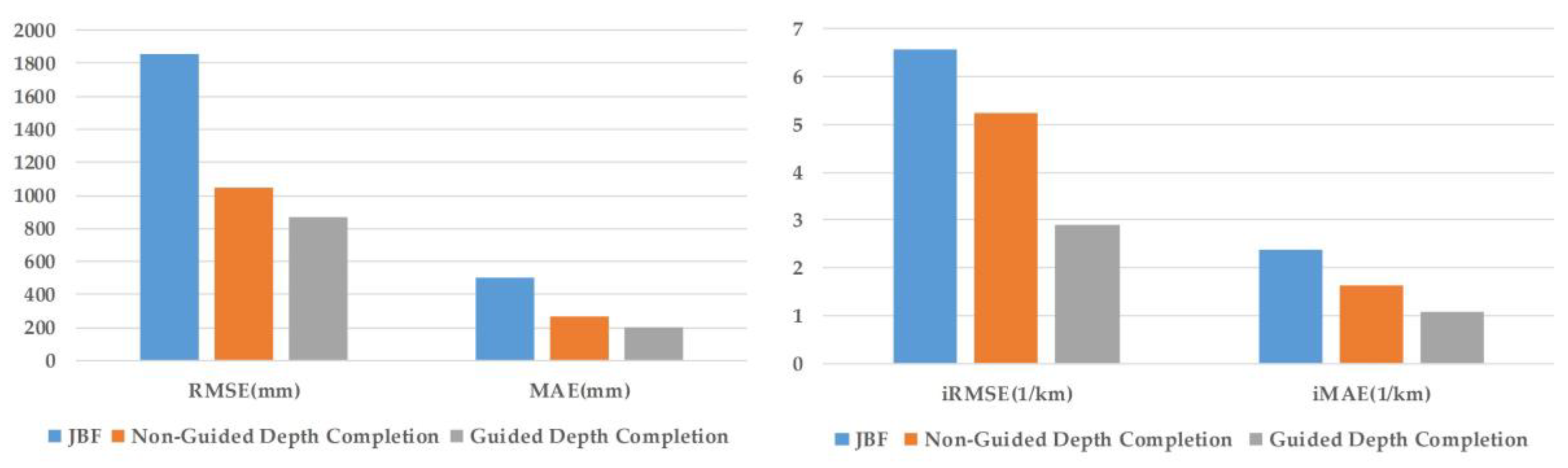
3.1. Depth Completion Experiment
3.2. Vehicle Detection and Fusion Experiment
4. Conclusions
Author Contributions
Funding
Conflicts of Interest
References
- Ross, G.; Jeff, D.; Trevor, D.; Jitendra, M. Rich Feature Hierarchies for Accurate Object Detection and Semantic Segmentation. In Proceedings of the IEEE Conference on Computer Vision and Pattern Recognition (CVPR), Columbus, OH, USA, 24–27 June 2014; pp. 580–587. [Google Scholar]
- He, K.; Zhang, X.; Ren, S.; Sun, J. Spatial pyramid pooling in deep convolutional networks for visual recognition. IEEE Trans. Pattern Anal. Mach. Intell. 2015, 37, 1904–1916. [Google Scholar] [CrossRef] [PubMed]
- Ross, G. Fast R-CNN. In Proceedings of the 2015 IEEE International Conference on Computer Vision (ICCV), Santiago, Chile, 7–13 December 2015; pp. 1440–1448. [Google Scholar]
- Ren, S.; He, K.; Girshick, R.; Sun, J. Faster R-CNN: Towards Real-Time Object Detection with Region Proposal Networks. IEEE Trans Patt. Anal. Mach. Intell. 2017, 39, 1137–1149. [Google Scholar] [CrossRef] [PubMed]
- Cai, Z.; Fan, Q.; Feris, R.S.; Vasconcelos, N. A unified multi-scale deep convolutional neural network for fast object detection. In Proceedings of the EUropean Conference on Computer Vision, Amsterdam, The Netherlands, 8–16 October 2016; pp. 354–370. [Google Scholar]
- Xiang, Y.; Choi, W.; Lin, Y.; Savarese, S. Subcategory-aware convolutional neural networks for object detection. In Proceedings of the IEEE Winter Conference on Applications Computer Vision (WACV), Santa Rosa, CA, USA, 27–29 March 2017; pp. 924–933. [Google Scholar]
- Chen, X.; Kundu, K.; Zhu, Y.; Berneshawi, A.; Ma, H.; Fidler, S.; Urtasun, R. 3D Object Proposals for Accurate Object Class Detection. In Proceedings of the 29th Annual Conference on Neural Information Processing Systems (NIPS), Montreal, QC, Canada, 7–12 December 2015; pp. 424–432. [Google Scholar]
- Chen, X.; Kundu, K.; Zhang, Z.; Ma, H.; Fidler, S.; Urtasun, R. Monocular 3d Object Detection for Autonomous Driving. In Proceedings of the IEEE Conference on Computer Vision and Pattern Recognition (CVPR), Las Vegas, NV, USA, 26 June–1 July 2016; pp. 2147–2156. [Google Scholar]
- Liu, W.; Anguelov, D.; Erhan, D.; Szegedy, C.; Reed, S.; Fu, C.Y.; Berg, A.C. SSD: Single Shot MultiBox Detector. In Proceedings of the 14th European Conference ECCV 2016, Amsterdam, The Netherlands, 11–14 October 2016; pp. 21–37. [Google Scholar]
- Lin, T.-Y.; Goyal, P.; Girshick, R.; He, K.; Dollar, P. Focal Loss for Dense Object Detection. In Proceedings of the IEEE International Conference on Computer Vision, Venice, Italy, 22–29 October 2017; pp. 2999–3007. [Google Scholar]
- Redmon, J.; Divvala, S.; Girshick, R.; Farhadi, A. You only look once: Unified, real-time object detection. In Proceedings of the IEEE Conference on Computer Vision and Pattern Recognition, Las Vegas, NV, USA, 27–30 June 2016; pp. 779–788. [Google Scholar]
- Zhou, Y.; Tuzel, O. VoxelNet: End-to-End Learning for Point Cloud Based 3D Object Detection. In Proceedings of the IEEE Conference on Computer Vision and Pattern Recognition (CVPR), Salt Lake City, UT, USA, 18–22 June 2018; pp. 4490–4499. [Google Scholar]
- Asvadi, A.; Premebida, C.; Peixoto, P.; Nunes, U. 3D Lidar-based static and moving obstacle detection in driving environments: An approach based on voxels and multi-region ground planes. Robot. Auton. Syst. 2016, 83, 299–311. [Google Scholar] [CrossRef]
- Sualeh, M.; Kim, G.W. Dynamic multi-lidar based multiple object detection and tracking. Sensors 2019, 19, 1474. [Google Scholar] [CrossRef]
- Brummelen, J.V.; O’Brien, M. Autonomous vehicle perception: The technology of today and tomorrow. Transp. Res. C. 2018, 89, 384–406. [Google Scholar] [CrossRef]
- Garcia, F.; Martin, D.; De La Escalera, A.; Armingol, J.M. Sensor fusion methodology for vehicle detection. IEEE Intell. Transp. Syst. Mag. 2017, 9, 123–133. [Google Scholar] [CrossRef]
- Gao, H.; Cheng, B.; Wang, J.; Li, K.; Zhao, J.; Li, D. Object classification using cnn-based fusion of vision and lidar in autonomous vehicle environment. IEEE Trans. Ind. Inf. 2018, 14, 4224–4231. [Google Scholar] [CrossRef]
- Chen, X.; Ma, H.; Wan, J.; Li, B.; Xia, T. Multi-view 3D Object Detection Network for Autonomous Driving. In Proceedings of the 2017 IEEE Conference on Computer Vision and Pattern Recognition (CVPR), Honolulu, HI, USA, 21–26 July 2017. [Google Scholar]
- Matti, D.; Ekenel, H.K.; Thiran, J.-P. Combining LiDAR Space Clustering and Convolutional Neural Networks for Pedestrian Detection. In Proceedings of the 14th IEEE International Conference on Advanced Video and Signal Based Surveillance (AVSS), Lecce, Italy, 29 August–1 September 2017. [Google Scholar]
- Wang, H.; Lou, X.; Cai, Y.; Li, Y.; Chen, L. Real-Time Vehicle Detection Algorithm Based on Vision and Lidar Point Cloud Fusion. J. Sens. 2019, 2019, 8473980. [Google Scholar] [CrossRef]
- De Silva, V.; Roche, J.; Kondoz, A. Robust fusion of LiDAR and wide-angle camera data for autonomous mobile robots. Sensors 2018, 18, 2730. [Google Scholar] [CrossRef]
- Premebida, C.; Carreira, J.; Batista, J.; Nunes, U. Pedestrian detection combining RGB and dense LIDAR data. In Proceedings of the IEEE/RSJ International Conference on Intelligent Robots and Systems, Chicago, IL, USA, 14–18 September 2014; pp. 4112–4117. [Google Scholar]
- Oh, S.I.; Kang, H.B. Object Detection and Classification by Decision-Level Fusion for Intelligent Vehicle Systems. Sensors 2017, 17, 207. [Google Scholar] [CrossRef]
- Chavez-Garcia, R.O.; Aycard, O. Multiple sensor fusion and classification for moving object detection and tracking. IEEE Trans. Intell. Transp. Syst. 2016, 17, 525–534. [Google Scholar] [CrossRef]
- Redmon, J.; Farhadi, A. YOLOv3: An Incremental Improvement. arXiv 2018, arXiv:1804.02767. [Google Scholar]
- Liu, W.; Jia, S.; Li, P.; Chen, X. An MRF-Based Depth Upsampling: Upsample the Depth Map With Its Own Property. IEEE Signal Process. Lett. 2015, 22, 1708–1712. [Google Scholar] [CrossRef]
- Kopf, J.; Cohen, M.F.; Lischinski, D.; Uyttendaele, M. Joint bilateral upsampling. Acm Trans. Graph. 2007, 26, 96. [Google Scholar] [CrossRef]
- Yang, Q.; Yang, R.; Davis, J.; Nistér, D. Spatial-Depth Super Resolution for Range Images. In Proceedings of the 2007 IEEE Computer Society Conference on Computer Vision and Pattern Recognition (CVPR), Minneapolis, MN, USA, 18–23 June 2007; pp. 1–8. [Google Scholar]
- Premebida, C.; Garrote, L.; Asvadi, A.; Ribeiro, P.; Nunes, U. High-resolution LIDAR-based Depth Mapping using Bilateral Filter. In Proceedings of the IEEE international conference on intelligent transportation systems (ITSC), Rio de Janeiro, Brazil, 1–4 November 2016; pp. 2469–2474. [Google Scholar]
- Ashraf, I.; Hur, S.; Park, Y. An Investigation of Interpolation Techniques to Generate 2D Intensity Image From LIDAR Data. IEEE Access 2017, 5, 8250–8260. [Google Scholar] [CrossRef]
- Ferstl, D.; Reinbacher, C.; Ranftl, R.; Ruether, M.; Bischof, H. Image guided depth upsampling using anisotropic total generalized variation. In Proceedings of the IEEE International Conference on Computer Vision (ICCV), Sydney, Australia, 1–8 December 2013; pp. 993–1000. [Google Scholar]
- Hsieh, H.Y.; Chen, N. Recognising daytime and nighttime driving images using Bayes classifier. IET Intell. Transp. Syst. 2012, 6, 482–493. [Google Scholar] [CrossRef]
- Redmon, J.; Farhadi, A. YOLO9000: Better, faster, stronger. arXiv 2016, arXiv:1612.08242. [Google Scholar]
- Tang, H.; Su, Y.; Wang, J. Evidence theory and differential evolution based uncertainty quantification for buckling load of semi-rigid jointed frames. Sadhana 2015, 40, 1611–1627. [Google Scholar] [CrossRef]
- Wang, J.; Liu, F. Temporal evidence combination method for multi-sensor target recognition based on DS theory and IFS. J. Syst. Eng. Electron. 2017, 28, 1114–1125. [Google Scholar]
- Jousselme, A.-L.; Grenier, D.; Bossé, É. A new distance between two bodies of evidence. Inf. Fusion 2001, 2, 91–101. [Google Scholar] [CrossRef]
- Han, D.; Deng, Y.; Liu, Q. Combining belief functions based on distance of evidence. Decis. Support Syst. 2005, 38, 489–493. [Google Scholar]
- Geiger, A.; Lenz, P.; Urtasun, R. Are we ready for autonomous driving? The KITTI vision benchmark suite. In Proceedings of the 2012 IEEE Conference on CVPR, Providence, RI, USA, 16–21 June 2012; pp. 3354–3361. [Google Scholar]
- Sun, P.; Kretzschmar, H.; Dotiwalla, X.; Chouard, A.; Patnaik, V.; Tsui, P.; Guo, J.; Zhou, Y.; Chai, Y.; Caine, B.; et al. Scalability in Perception for Autonomous Driving: Waymo Open Dataset. arXiv 2019, arXiv:1912.04838. [Google Scholar]
- Everingham, M.; Van Gool, L.; Williams, C.K.; Winn, J.; Zisserman, A. The pascal visual object classes (voc) challenge. Int. J. Comput. Vis. 2010, 88, 303–338. [Google Scholar] [CrossRef]
- Jeong, J.; Park, H.; Kwak, N. Enhancement of SSD by concatenating feature maps for object detection. arXiv 2017, arXiv:1705.09587v1. [Google Scholar]


| Method | RMSE (mm) | MAE (mm) | iRMSE (1/km) | iMAE (1/km) |
|---|---|---|---|---|
| Joint bilateral upsampling (JBU) | 1856.83 | 501.64 | 6.58 | 2.38 |
| Non-guided depth completion | 1046.21 | 266.50 | 5.23 | 1.63 |
| Guided depth completion | 865.62 | 200.7 | 2.91 | 1.09 |
| Method | Easy | Moderate | Hard |
|---|---|---|---|
| Guided Depth Completion | 75.13% | 62.34% | 51.26% |
| color | 82.17% | 77.53% | 68.47% |
| Fusion | 85.62% | 80.16% | 70.19% |
| Color | Non-Guided Depth Completion | Fusion | |
|---|---|---|---|
| AP | 65.47% | 60.13% | 69.02% |
| Method | KITTI | Waymo | Time | Environment | ||
|---|---|---|---|---|---|---|
| Easy | Moderate | Hard | Night | |||
| Faster R-CNN [4] | 87.90% | 79.11% | 70.19% | 68.37% | 2s | GPU@3.5Ghz |
| MV3D [18] | 89.80% | 79.76% | 78.61% | / | 0.24s | GPU@2.5Ghz |
| 3DVP | 81.46% | 75.77% | 65.38% | 63.84% | 40s | GPU@3.5Ghz |
| 3DOP [7] | 90.09% | 88.34% | 78.39% | 77.42% | 3s | GPU@2.5Ghz |
| MS-CNN [5] | 90.03% | 89.02% | 76.11% | 73.57% | 0.4s | GPU@2.5Ghz |
| Yolov2 [32] | 74.35% | 62.65% | 53.23% | 56.45% | 0.03s | GPU@3.5Ghz |
| Yolov3 [24] | 82.17% | 77.53% | 68.47% | 65.47% | 0.04s | GPU@2.5Ghz |
| R-SSD [41] | 88.13% | 82.37% | 71.73% | / | 0.08s | GPU@2.5Ghz |
| SubCat | 81.45% | 75.46% | 59.71% | / | 0.7s | GPU@3.5Ghz |
| Mono3D [8] | 90.27% | 87.86% | 78.09% | 77.51% | 4.2s | GPU@2.5Ghz |
| SubCNN [6] | 90.75% | 88.86% | 79.24% | / | 2s | GPU@3.5Ghz |
| Fusion | 85.62% | 80.46% | 70.19% | 69.02% | 0.057s | GPU@2.5Ghz |
© 2020 by the authors. Licensee MDPI, Basel, Switzerland. This article is an open access article distributed under the terms and conditions of the Creative Commons Attribution (CC BY) license (http://creativecommons.org/licenses/by/4.0/).
Share and Cite
Guan, L.; Chen, Y.; Wang, G.; Lei, X. Real-Time Vehicle Detection Framework Based on the Fusion of LiDAR and Camera. Electronics 2020, 9, 451. https://doi.org/10.3390/electronics9030451
Guan L, Chen Y, Wang G, Lei X. Real-Time Vehicle Detection Framework Based on the Fusion of LiDAR and Camera. Electronics. 2020; 9(3):451. https://doi.org/10.3390/electronics9030451
Chicago/Turabian StyleGuan, Limin, Yi Chen, Guiping Wang, and Xu Lei. 2020. "Real-Time Vehicle Detection Framework Based on the Fusion of LiDAR and Camera" Electronics 9, no. 3: 451. https://doi.org/10.3390/electronics9030451
APA StyleGuan, L., Chen, Y., Wang, G., & Lei, X. (2020). Real-Time Vehicle Detection Framework Based on the Fusion of LiDAR and Camera. Electronics, 9(3), 451. https://doi.org/10.3390/electronics9030451