Regional Short-Term PV Power Forecasting Based on Graph Convolution and Transformer Networks

Abstract

Accurate short-term photovoltaic (PV) power forecasting is essential for power system scheduling and market operations. Existing studies have shown the value of numerical weather prediction (NWP), graph-based spatial modeling, and temporal sequence learning, but the boundary of their contributions remains fragmented across many practical forecasting frameworks. In particular, adjacent multi-point NWP information is often not explicitly organized according to its spatial relationships, while historical similar-day power is rarely integrated with graph-structured meteorological features in a unified model. To address this gap, this study develops a short-term PV power forecasting framework that combines multi-point NWP graph construction with similar-day-guided Transformer fusion. First, predicted irradiance from the target site and neighboring NWP points is organized as a graph, and a Graph Convolutional Network (GCN) is used to extract local spatial meteorological features. Second, similar days are identified through a two-stage selection strategy based on Euclidean distance and Pearson correlation, and the corresponding historical power sequences are aggregated as temporal guidance. Finally, the graph-extracted NWP features, similar-day power, and predicted humidity are fused by a Transformer-based temporal modeling module to generate day-ahead PV power forecasts. Experimental results show that the proposed framework outperforms TCN-Transformer, Transformer, GCN, LSTM, and BP on the studied dataset, and maintains favorable performance on additional PV stations. These results indicate that the joint integration of graph-structured multi-point NWP information and historical similar-day power is effective for short-term PV power forecasting.

1. Introduction

1.1. Background and Motivation

The rapid growth of photovoltaic (PV) generation has increased the need for accurate short-term forecasting in power system dispatch, reserve allocation, and electricity market operations. According to the International Energy Agency (IEA), renewable energy is expected to continue expanding substantially in the coming years, with PV playing an increasingly important role in the future electricity mix [1]. The increasing penetration of PV generation also amplifies the operational challenges caused by output uncertainty.

However, PV power output is highly sensitive to meteorological conditions, especially solar irradiance, cloud evolution, temperature, and humidity. As a result, PV generation exhibits significant intermittency and fluctuation, which may adversely affect grid security, scheduling efficiency, and market decision-making [2,3]. As PV power generation continues to develop and expand in scale, these issues are expected to become increasingly severe. In view of this, PV power forecasting has emerged as an effective measure to address these challenges. By accurately forecasting future PV generation, grid operators can proactively plan scheduling, allocate conventional energy generation and energy storage resources more effectively, and ensure the balance of power supply and demand [4].

1.2. Literature Review

In recent years, photovoltaic (PV) power forecasting has attracted extensive attention, and a large body of research has been developed across different forecasting horizons. In general, PV forecasting can be divided into ultra-short-term (15 min to 4 h), short-term (4 h to 3 days), and medium- to long-term (3 days to 1 month). Among them, ultra-short-term forecasting mainly supports real-time dispatch, whereas medium- to long-term forecasting is more relevant to planning and investment decisions [5]. Compared with these two forecasting horizons, short-term forecasting is more directly associated with day-ahead scheduling and operational optimization, such as generation planning and reserve arrangement. Therefore, improving short-term PV forecasting accuracy is of practical importance for mitigating PV output uncertainty and enhancing power system reliability [6].

For short-term PV forecasting, future meteorological information is indispensable because the forecasting horizon is sufficiently long that the direct temporal dependence of historical PV power becomes relatively weaker than that in ultra-short-term forecasting. Numerical Weather Prediction (NWP) provides key exogenous variables for the forecast day, including solar irradiance, cloud cover, temperature, and humidity, all of which strongly affect PV output. For this reason, many short-term PV forecasting studies have incorporated NWP data into their models [7,8]. For instance, Ref. [9] showed that combining power data with NWP information can alleviate forecasting errors caused by incomplete historical power data, while Ref. [10] compared several models using day-ahead NWP data from 23 PV sites in Finland and confirmed that meteorological inputs substantially influence forecasting performance. Similarly, Ref. [11] proposed an improved PV forecasting model based on Long Short-Term Memory and self-attention, demonstrating that effective use of weather forecast data can noticeably improve prediction accuracy. Taken together, these studies consistently indicate that NWP is a necessary information source for short-term PV forecasting. However, their common limitation is that they mostly rely on raw NWP data from a single prediction source. Since NWP itself inevitably contains forecast errors, the use of only one source may directly propagate these errors into the final PV forecasting results [12].

To reduce the influence of NWP uncertainty, another line of research has focused on NWP correction [13,14]. Existing methods mainly fall into two categories: statistical post-processing based on historical forecast errors, and mapping-based correction that links raw NWP outputs with observed meteorological measurements. These methods are valuable because they attempt to improve the quality of meteorological inputs before power forecasting is performed. Nevertheless, their improvement is often limited by the fact that they mainly model the temporal deviation of NWP data at a single location. In other words, although they can partially reduce local forecast bias, they do not explicitly describe the spatial consistency or interaction among neighboring meteorological prediction points. As a result, their ability to represent complex and rapidly changing regional weather conditions remains limited.

Recognizing this limitation, some studies have attempted to introduce multi-source NWP information into forecasting models so as to reduce dependence on a single prediction source. For instance, Refs. [15,16] employed ensemble predictions from 20 and 51 different NWP sources, respectively, to improve short-term wind power forecasting. Likewise, Ref. [17] fed multi-point NWP data into a Convolutional Neural Network to enrich meteorological inputs by exploiting the spatial relevance among wind farms. These studies suggest that increasing the diversity of meteorological inputs is beneficial, especially when the uncertainty of a single NWP source is high. However, in most cases, multi-source or multi-point NWP data are still treated as ordinary multidimensional inputs connected through predefined rules. This means that the spatial organization of meteorological fields is only weakly represented, and the intrinsic correlations among NWP points are not explicitly modeled. In contrast, Ref. [18] showed that Ensemble NWP combined with bias correction can significantly reduce PV forecast errors, which further implies that the way meteorological information is organized and corrected is critical to forecasting performance. Therefore, the key issue is not only how many NWP sources are used, but also whether the spatial relationship among them is effectively represented.

Graph Convolutional Networks (GCNs) provide a promising way to address this issue because they are well suited for modeling graph-structured data and non-Euclidean spatial relationships [19]. Existing studies [20,21,22,23,24] have mainly constructed graphs using spatial correlations among PV stations or historical power series within the same region, and these methods have generally achieved better forecasting performance than conventional models. Their success indicates that explicitly encoding spatial dependence is beneficial for renewable energy forecasting. However, most of these graph-based studies focus on the correlation structure among PV stations themselves, rather than among adjacent NWP points. As a result, they do not directly address how the spatial relationships embedded in meteorological forecast sources can be exploited for short-term PV forecasting. This issue is particularly important because neighboring NWP points may contain complementary meteorological information that cannot be sufficiently represented by station-level graph construction alone. Therefore, constructing a graph directly from multi-point NWP data offers a more natural way to characterize local meteorological spatial correlations around the target PV station.

Nevertheless, spatial meteorological representation alone is still insufficient for accurate short-term PV forecasting. In addition to spatial dependence among NWP points, PV generation also exhibits strong temporal regularity under similar weather conditions. For this reason, historical similar-day power has been widely regarded as valuable prior information, as it can preserve realistic generation patterns that are difficult to infer from meteorological variables alone. Meanwhile, Transformer-based models have shown strong capability in long-sequence modeling and heterogeneous feature fusion [25,26], and have gradually been applied to PV forecasting to improve multimodal data integration and long-term dependency extraction [27,28,29]. These studies suggest that the Transformer is well suited for capturing the temporal dependencies hidden in historical and forecast-related features. However, most existing studies either emphasize spatial modeling or focus mainly on temporal sequence learning, and few have explicitly considered how graph-extracted multi-point NWP features and historical similar-day power can be jointly integrated within a unified framework. This gap motivates the present study, in which a GCN is used to extract spatial information from adjacent NWP points, while similar-day power and a Transformer are introduced to complement this spatial representation with realistic historical patterns and long-range temporal dependencies.

1.3. Contributions

In summary, existing studies have demonstrated the importance of NWP inputs, spatial dependence modeling, and temporal feature extraction in PV power forecasting. However, for short-term PV forecasting, two issues remain insufficiently addressed. First, the spatial relationships among adjacent NWP points are seldom explicitly modeled, even though such information may help describe local meteorological variations around the target PV station. Second, historical similar-day power, which contains realistic generation patterns under comparable weather conditions, is rarely integrated with graph-structured multi-point NWP information within a unified forecasting framework. To address these issues, this study develops a short-term PV power forecasting framework based on multi-point NWP data, GCN-based spatial feature extraction, and Transformer-based temporal fusion.

The main contributions of this study are summarized as follows:

(1)

A graph representation is constructed for adjacent multi-point NWP irradiance data, allowing local spatial correlations among neighboring prediction points to be explicitly encoded before temporal forecasting.

(2)

Historical similar-day power is introduced together with predicted meteorological information for the target day, so that the model can use both realistic historical generation patterns and future weather-related inputs in short-term PV forecasting.

(3)

A unified GCN-Transformer forecasting framework is developed to combine graph-extracted multi-point NWP features, historical similar-day power, and predicted meteorological data, thereby enabling joint modeling of spatial meteorological dependence and temporal generation patterns.

The remainder of this paper is organized as follows. Section 2 introduces the principles and methods of the PV power forecasting model. Section 3 provides a detailed description of the experimental setup. Section 4 presents an analysis of the experimental results. Section 5 offers a discussion, and finally, Section 6 concludes the paper with a summary and outlook.

2. Methodology

2.1. The Framework of the Proposed Research

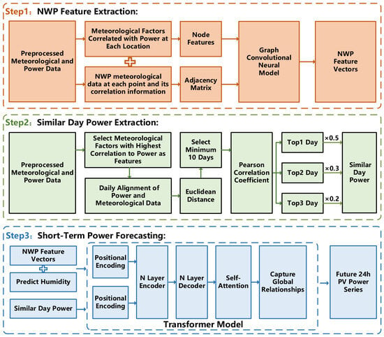
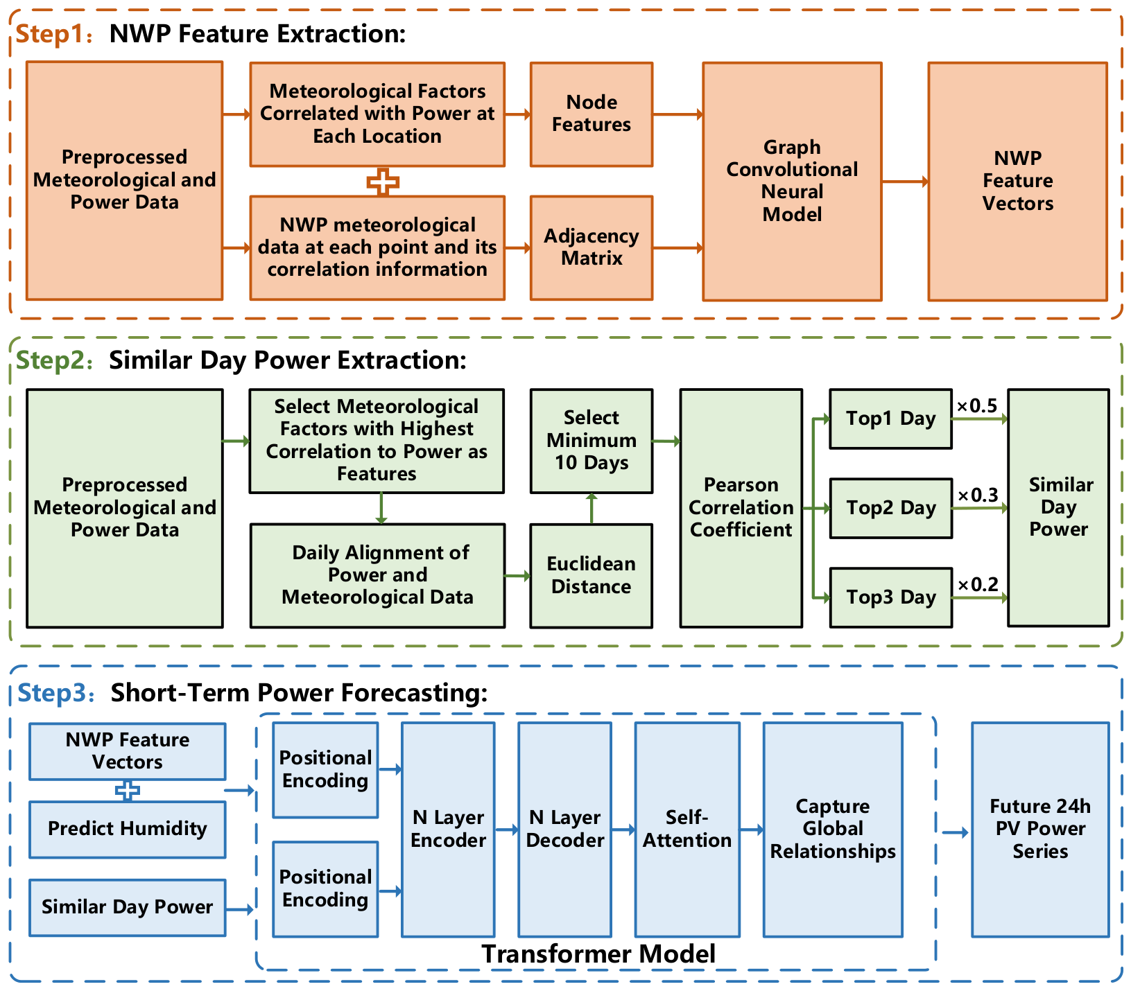
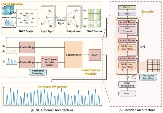
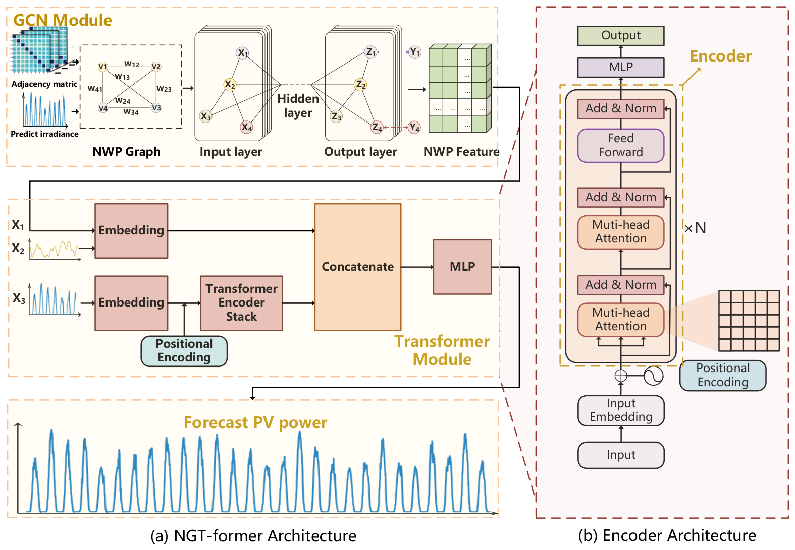
This paper proposes a short-term PV power forecasting model based on NWP and GCN-Transformer (NGT-former), with the overall technical framework shown in Figure 1.

Figure 1. The framework of the proposed method.

(1)

First, NWP data for the target PV power station and its surrounding four prediction locations are collected. The most relevant meteorological data that correlate strongly with power generation are identified. A graph network is constructed using the meteorological data from different NWP locations and their correlation information. GCN is used to encode spatial relationships and extract feature vectors from the NWP data.

(2)

The dataset is divided into training and test sets in a certain proportion. In all datasets, based on the predicted irradiance data of the target day and historical days, the most similar days in the training set are selected using a two-stage extraction method. The historical power data of these similar days are weighted and averaged, then added to the input data as new historical power data.

(3)

The output feature vectors from the GCN model, historical similar-day power, and the predicted humidity data for the target day are input into the Transformer model. This introduces dual data streams: the exogenous future variables data stream (NWP feature vectors, predicted humidity) and the historical similar-day power data stream. Through the self-attention mechanism of the Transformer, global dependencies between the inputs and outputs are extracted, ultimately yielding the PV power forecast for the target day.

2.2. Correlation Analysis

The Pearson correlation coefficient is a measure of the linear relationship between two variables. It returns a value between −1 and +1, where +1 indicates perfect positive correlation, −1 indicates perfect negative correlation, and 0 indicates no linear relationship. For two sets of data, the Pearson correlation coefficient is calculated using the following formula:

$$r_{AB}={\displaystyle \frac{{\displaystyle \sum _{i=1}^n}(A_i-\overline{A})(B_i-\overline{B})}{\sqrt{{\displaystyle \sum _{i=1}^n}{(A_i-\overline{A})}^2}\sqrt{{\displaystyle \sum _{i=1}^n}{(B_i-\overline{B})}^2}}}$$

(1)

Here, $\overline{A}$ and $\overline{B}$ represent the average values of series A and B, respectively.

In this research, the Pearson correlation coefficient was calculated to determine the relationship between each predicted meteorological variable at different points and the PV power output of the target station, as shown in Table 1.

Table 1. Pearson correlation coefficient between meteorological data and PV power.

Point	Irradiance	Humidity	Cloud Cover	Wind Speed	Wind Direction	Air Pressure
1	0.9118	−0.4008	−0.1052	−0.1020	−0.0782	−0.0304
2	0.9116	−0.4002	−0.1053	−0.1121	−0.0789	−0.0386
3	0.9122	−0.3988	−0.1120	−0.1012	−0.0812	−0.0313
4	0.9120	−0.4016	−0.1010	−0.0986	−0.0712	−0.0295

The correlation analysis shows that predicted irradiance at all four NWP points has a strong linear relationship with the PV power output of the target station. Predicted humidity also exhibits a certain degree of correlation with PV power, whereas other meteorological variables show relatively weak or negligible correlations. Therefore, to better account for the influence of meteorological conditions on PV power generation, predicted humidity is included as an additional input variable in power forecasting models.

2.3. Spatial and Temporal Correlation Between Adjacent NWP Points

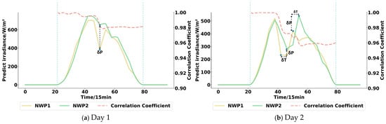
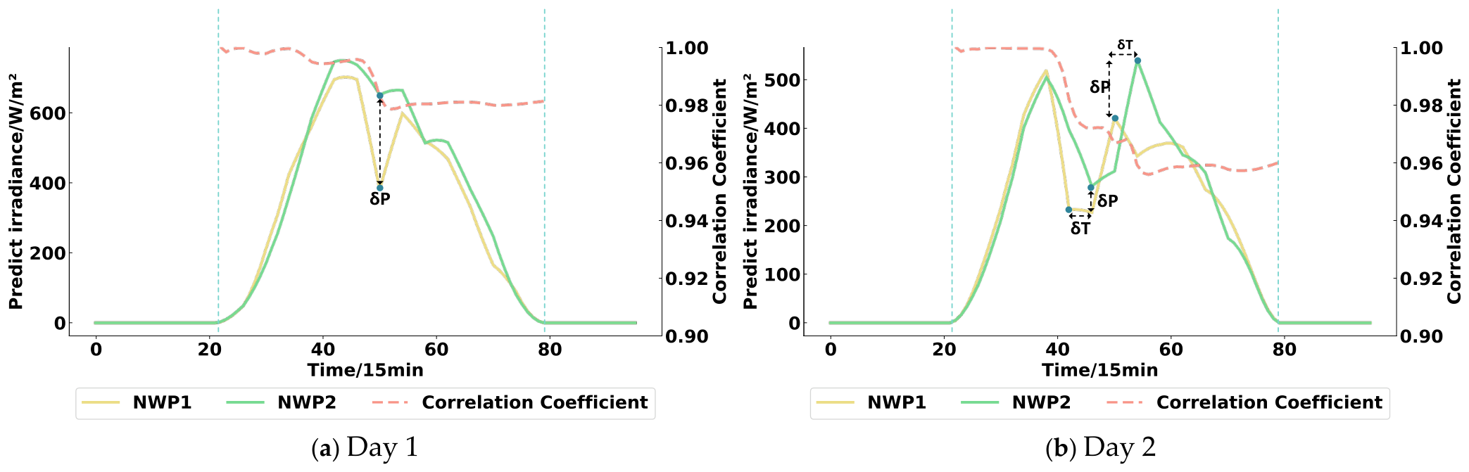
In a local region, predicted irradiance series from adjacent NWP points often show similar overall evolution because the underlying meteorological field is spatially continuous. This property is referred to here as spatial similarity. At the same time, due to cloud movement and local meteorological variation, neighboring irradiance series may also exhibit time shifts and peak differences. In this study, these lagged and amplitude-related differences are described as temporal correlation. A related concept has also been discussed in previous studies on adjacent PV stations, where the spatiotemporal association among neighboring stations was used to describe the similarity and temporal interaction of PV-related signals under shared meteorological conditions [30]. Although that definition was proposed for adjacent PV stations rather than adjacent NWP points, it provides useful support for the present study. Figure 2 illustrates this phenomenon using irradiance sequences from two adjacent NWP points. It can be observed that the predicted irradiance at these two points exhibits similar temporal variation patterns; the Pearson coefficient is high when the PV output is not zero. However, dynamic cloud changes lead to peak differences (δP) and time lags (δT) between the irradiance predictions, visually demonstrating the interplay of temporal and spatial correlations. By capturing the spatiotemporal correlations of meteorological data between adjacent NWP points, it is possible to enhance the model’s responsiveness to complex weather changes. Additionally, this understanding can facilitate the optimal allocation of resources for PV power stations based on specific regional weather patterns and these spatiotemporal relationships, thereby promoting the effective utilization of renewable energy and ensuring the stable operation of the power grid.

Figure 2. Spatial and temporal correlation of predicted irradiance at adjacent NWP points.

2.4. Two-Stage Similar-Day PV Power Selection

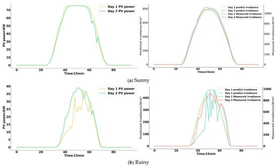
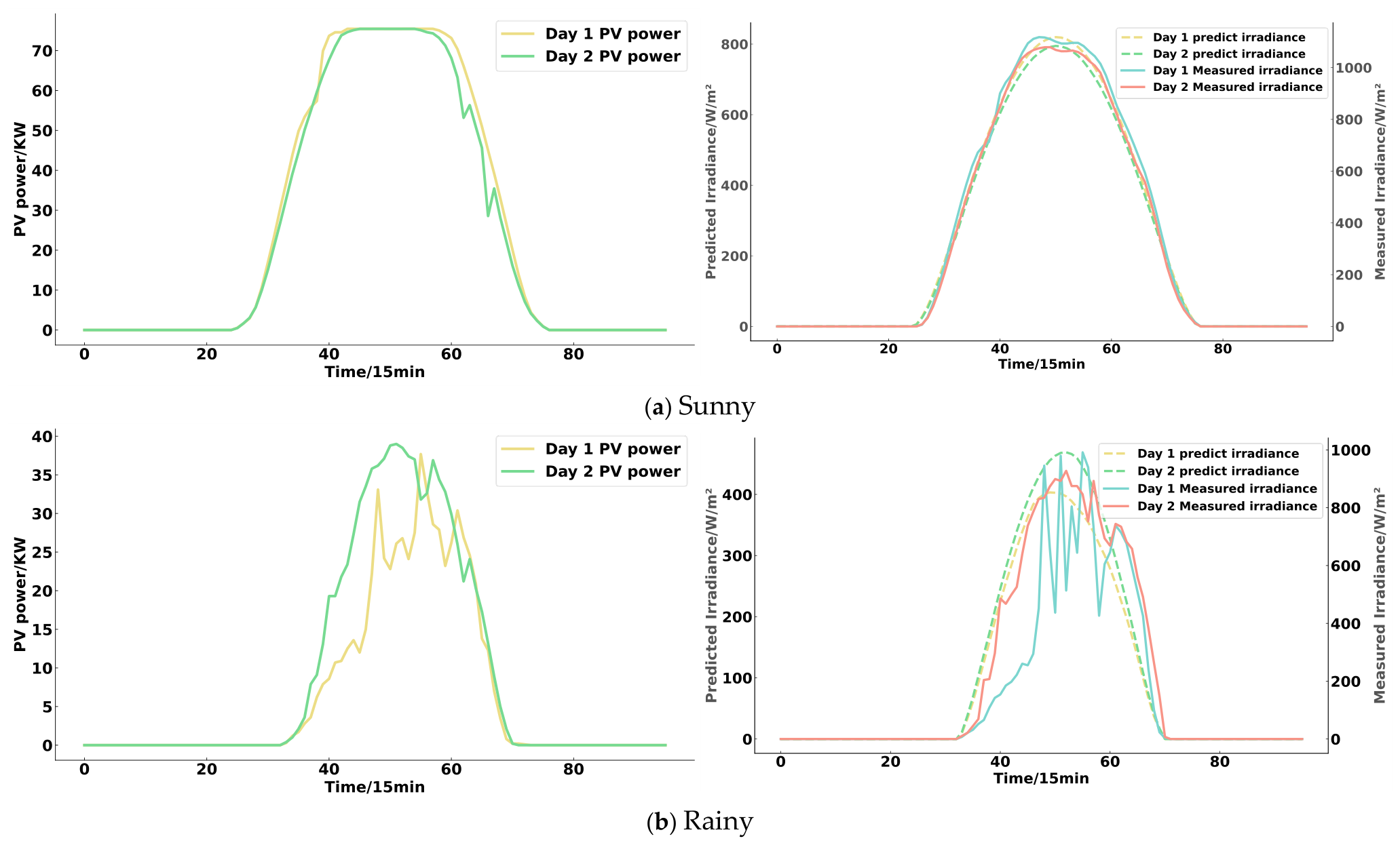
Due to natural factors such as seasonal changes, the alternation of day and night, and various weather types, solar radiation intensity exhibits certain periodicity and uncertainty. Under clear sky conditions, solar radiation intensity follows a more regular pattern with high similarity; however, under cloudy or rainy conditions, solar radiation is heavily influenced by cloud cover, resulting in less regularity and lower similarity. Figure 3 illustrates two days with similar predicted irradiance under both clear and rainy weather conditions. It has been observed that when the predicted irradiance is similar, the measured irradiance also shows a certain degree of similarity, which in turn leads to a certain level of similarity in the actual power output.

Figure 3. Predicted irradiance and PV power under similar weather conditions.

Based on these observations, this research identifies historical days with highly similar predicted irradiance to the target forecast day to retrieve the corresponding measured power outputs for these similar days. These similar-day power outputs are incorporated as inputs to the power forecasting model to capture the actual power generation patterns of these similar days, thereby improving the accuracy of PV power forecasting [31,32].

The selection of similar days is based on the similarity of meteorological data characteristics between historical days and the target forecast day. There are numerous factors influencing PV power, with varying degrees of impact on the output. By selecting the most relevant factors, we can more accurately capture the relationship between power generation and its influencing factors. According to the correlation analysis results, the predicted irradiance at each point shows the most significant relationship with PV power. Therefore, in this research, predicted irradiance is chosen as the feature for selecting similar days.

Since the objective of this research is short-term PV power forecasting, similar days are selected based on the entire power output sequence of the target day. First, the Euclidean distance and Pearson correlation coefficient between the predicted irradiance of the target day and all candidate days are computed. Euclidean distance is a commonly used distance metric to measure the straight-line distance between two points. By using Euclidean distance, we can identify the day with predicted irradiance values most similar to the target day. Let the two sets of predicted irradiance data be $A=(A_1,A_2,\dots ,A_n)$ and $B=(B_1,B_2,\dots ,B_n)$. The Euclidean distance between them is calculated as:

$$d(A,B)=\sqrt{\sum _{i=1}^n{(A_i-B_i)}^2}$$

(2)

where n is the number of data points in a day. The smaller the Euclidean distance, the closer the two sets of data are.

The Pearson correlation coefficient can be used to evaluate the trend similarity between the irradiance sequence of a historical day and that of the target forecast day. Even when the absolute irradiance values differ, two days may still exhibit similar power generation behavior if their variation trends are consistent. This is particularly important under cloudy or rainy conditions, where irradiance fluctuations are more irregular and Euclidean distance alone may not be sufficient to identify truly similar days. Therefore, Euclidean distance and Pearson correlation were jointly employed in this study to balance numerical similarity and trend similarity, thereby improving the reliability of similar-day selection, which is also consistent with previous similar-day PV forecasting studies [33].

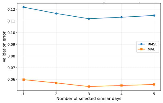
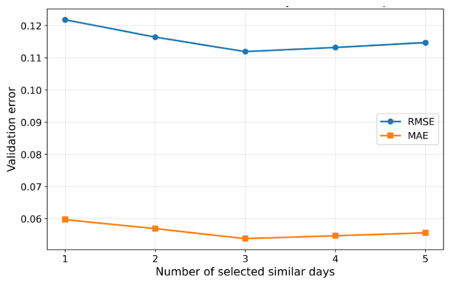
To determine the appropriate number of similar days used in the PV power forecasting model: Firstly, the 10 closest candidate days were selected according to Euclidean distance; the initial candidate size was fixed at 10 to provide a balance between recall and computational cost. A smaller candidate pool may prematurely exclude days with similar trend patterns but moderate value deviations, whereas a much larger candidate pool may introduce many weakly related samples into the second-stage correlation screening. Then the top m days were retained based on the Pearson correlation, where m was set from 1 to 5. The corresponding error results are shown in Figure 4. It can be observed that the error decreases as the number of selected similar days increases from 1 to 3, and then gradually increases when more similar days are included. This indicates that selecting too few similar days makes the model more sensitive to the randomness of individual historical samples, whereas selecting too many similar days may introduce less representative samples and increase redundant information. Therefore, m = 3 was adopted in this study, since it achieved the lowest validation error among the compared settings while maintaining a reasonable computational cost.

Figure 4. Effect of the number of selected similar days on validation performance.

After determining that three similar days should be retained, their historical power sequences were combined using a fixed rank-based weighting strategy. Although the selected similar days vary across forecast dates, their roles remain stable after similarity ranking: the first-ranked similar day provides the most representative information, while the second- and third-ranked similar days serve as supplementary references. Therefore, the weights were assigned according to similarity rank rather than the identity of a specific historical day. A fixed weighting strategy was adopted instead of day-specific dynamic weights because dynamic weights could introduce additional sample-wise fluctuations and reduce the stability of the similar-day input. In this study, the fixed weights were not empirically assigned but derived from the present dataset based on the overall similarity statistics of the training set. Specifically, the Pearson similarity coefficients of the first-, second-, and third-ranked similar days were collected over the entire training set and then normalized to obtain the final weights. As a result, the fixed weights used in this paper were 0.5, 0.3, and 0.2, respectively.

2.5. GCN-Transformer Model

2.5.1. GCN Model

Due to the influence of weather processes, geographic location, and the spatial topology of meteorological stations, meteorological conditions differ across locations. Therefore, incorporating the spatial correlations of multi-point NWP data into the PV power forecasting model is crucial. However, traditional CNN models face limitations when dealing with non-Euclidean spatial data and cannot directly capture spatial relationships between different geographic locations. GCN, on the other hand, is effective at learning and representing graph-structured data by aggregating information from nodes and their neighbors through graph convolution operations [19,21,22]. Specifically, by utilizing the dependencies between nodes on the graph, GCN can capture the spatial correlations between multi-point NWP data and extract local structural features. Figure 5a illustrates the structure of the GCN model. Based on the correlation analysis results, predicted irradiance shows the strongest correlation with PV power among the considered meteorological variables. Therefore, predicted irradiance from the four NWP points is used as the node feature in the GCN module. Predicted humidity is not discarded; instead, it is introduced as an auxiliary exogenous variable in the Transformer branch. This design keeps the graph representation compact while still preserving additional meteorological information for temporal fusion.

Figure 5. NGT-former model framework.

To enable the GCN to process NWP data, graph modeling is conducted by analyzing the correlations of predicted irradiance across multiple NWP points within the region. NWP points in the region are represented as nodes, and the correlations between them are represented as weighted edges. The predicted irradiance at time t in the region can be represented as a spatiotemporal graph:

$${\dot{G}}_t=<V_t,E>$$

(3)

$$V_t=\left\{v_{i,t}\right\}(i=1,2,3,\dots ,n)$$

(4)

$$E=\left\{w_{ij}\right\}(i,j=1,2,3,\dots ,n)$$

(5)

where $V_t=\left\{v_{i,t}\right\}$ represents the set of NWP predicted irradiance data for all nodes in the spatiotemporal graph at time t; $E=\left\{w_{i,j}\right\}$ is the weighted adjacency matrix of the spatiotemporal graph; $w_{ij}$ is the weight coefficient between node v_i and node v_j.

Nodes v_i and v_j can only be connected if they have a high correlation. The weight coefficient between the nodes can be expressed as:

$$w_{i,j}=\left\{\begin{array}{cc}{e}^{-(v_i,v_j)},\hfill & r_{ij}>k\hfill \\ 0 ,\hfill & r_{ij}⩽k\hfill \end{array}\right.$$

(6)

where r_ij represents the correlation coefficient between two nodes, and (v_i, v_j) represents the Euclidean distance between the nodes. k is used to determine whether an edge should be retained according to the correlation between two NWP points. In this study, the pairwise Pearson correlation coefficients among the four NWP irradiance series were first calculated on the training set, and their median value was taken as a statistical reference for threshold selection. Several nearby candidate thresholds were further evaluated on the validation set. The final threshold was selected by jointly considering forecasting accuracy and graph sparsity, thereby filtering out weak correlations while preserving the main spatial dependencies among adjacent NWP points. After the threshold k was selected using the training and validation sets, it was kept fixed throughout the experiments. If r_ij > k, it indicates a high correlation between the two NWP points, and nodes v_i and v_j can be connected by an edge. If r_ij ≤ k, it means there is no connection between the nodes. It is worth noting that the adjacency matrix changes daily; therefore, it is a dynamic adjacency matrix.

The GCN is used to extract spatial features of each node in the NWP point-line topological graph. At the same time, the normalized Laplacian matrix is applied in the spectral domain, and the NWP graph structure is defined as:

$$L^2=I-D^{-{\displaystyle \frac{1}{2}}}E{D}^{{\displaystyle \frac{1}{2}}}$$

(7)

where $I$ represents the identity matrix, $E=\left\{w_{i,j}\right\}$ is the weighted adjacency matrix of the NWP predicted irradiance graph structure, $D=\left\{d_{i,i}\right\}\in R^{N\times N}$ is the degree matrix of the NWP predicted irradiance graph structure, where $d_{i,i}={\displaystyle \sum _j}{w}_{ij}$.

The normalized Laplacian matrix can be decomposed as $L=U\Lambda U^{\mathrm{T}}$, where $U\in {ℝ}^{N\times N}$ is the matrix composed of eigenvectors of $L$, $\Lambda =\left[{\lambda }_1,{\lambda }_2,\dots ,\lambda n\right]$ is the diagonal matrix composed of the eigenvalues of $L$. By simplifying the graph convolution operation, the graph convolution formula can be expressed as:

$$(X_m\ast \mathit{g})=\mathit{U}(({\mathit{U}}^{\mathrm{T}}\mathit{g})\odot ({\mathit{U}}^{\mathrm{T}}{\mathit{X}}_m))$$

(8)

where $X_m$ represents the input to the GCN module, $\mathit{g}$ is the convolution kernel, and $\odot$ denotes the Hadamard product. Using ${\mathit{g}}_{\theta }=U^{\mathrm{T}}\mathit{g}$ as the convolution kernel and $\theta \in {ℝ}^{N\times N}$, the graph convolution formula is expressed as:

$$(X_m\ast g)=U{g}_{\theta }{U}^{\mathrm{T}}{X}_m$$

(9)

Due to the high computational complexity of graph convolution, Chebyshev polynomials are used to approximate the convolution kernel to improve the efficiency of spatial feature extraction. The convolution kernel can be expressed as:

$${\mathit{g}}_{\theta }={\mathit{g}}_{\theta }(\Lambda )\approx \sum _{H=0}^{H-1}{\mathit{\theta }}_H{\mathit{T}}_H(\tilde{\Lambda })$$

(10)

where $\tilde{\Lambda }$ represents the scaled eigenvalue matrix of $\Lambda$, and $\tilde{\Lambda }={\displaystyle \frac{2\Lambda }{{\lambda }_{\max }}}-I$, where ${\lambda }_{\max }$ is the maximum eigenvalue of matrix $L$, ${\mathit{\theta }}_H$ represents the coefficient vector of the corresponding Chebyshev polynomial, and $T_H\left(\begin{array}{c}x\end{array}\right)$ represents the Chebyshev polynomial, which can be expressed as:

$$T_H(x)=2x{T}_{H-1}(x)-T_{H-2}(x)$$

(11)

where $T_0(x)=1,T_1(x)=x$, where H denotes the order of the Chebyshev polynomial.

By introducing the Chebyshev polynomial, the graph convolution formula can be transformed into:

$$g\ast x=\sum _{H=0}^{H-1}{\mathit{\theta }}_H{\mathit{T}}_H(\tilde{\mathit{L}})x$$

(12)

where $\tilde{\mathit{L}}={\displaystyle \frac{2\mathit{L}}{{\lambda }_{\max }}}-\mathit{I}=\mathit{U}\tilde{\mathit{L}}{\mathit{U}}^{\mathrm{T}}$.

By inputting the graph node information and the weighted adjacency matrix $E=\left\{w_{i,j}\right\}$ into the GCN module, the spatial convolution operation extracts the NWP feature vector.

2.5.2. Transformer Model

The Transformer model, proposed by Google in 2017, was initially applied to machine translation and is entirely based on the attention mechanism to model the global dependencies between the source and target language sequences. Unlike the standard encoder–decoder architecture commonly used in sequence generation tasks [34], the proposed model employs only the encoder part of the Transformer for continuous PV power regression. The encoder structure based on the Transformer model is shown in Figure 5b. The encoder is composed of several basic Transformer blocks (represented by the light-colored boxes in Figure 5b). The “N×” indicates that the blocks are stacked N times. Each Transformer block receives a sequence of vectors as input and outputs a sequence of vectors of the same length. In this Transformer model, the input sequence consists of NWP feature vectors, historical similar-day power, and predicted humidity, and the output sequence is the future 24 h PV power sequence. Specifically, the Transformer encoder first maps the input sequence into an embedding space and incorporates positional encoding. The embedded sequence is then passed through the stacked encoder blocks to capture long-range temporal dependencies within the historical similar-day power data. The output of the encoder is subsequently sent to the regression head. In the proposed framework, this encoded temporal representation is further fused with the meteorological feature branch before the final prediction is generated. In this way, the model combines the temporal regularity contained in historical similar-day power with the future meteorological information extracted from adjacent NWP points. The embedding layers used in the model serve as projections from the original input space to a higher-dimensional feature space and consist of a linear transformation followed by a nonlinear activation function. Through this design, the model includes three main components: the embedding layers, the Transformer encoder stack, and the final MLP-based regression module. This structure enables effective fusion of heterogeneous inputs and supports accurate short-term PV power forecasting.

The main model architecture is shown in Figure 5a. This study introduces a dual data stream mechanism to deeply integrate the characteristics of historical data streams with those of future exogenous data streams. Specifically, the model receives two main parts of input data: one is the historical similar-day power (X3), which is linearly transformed and activated into a high-dimensional space, followed by adding positional encoding to preserve the position information in the sequence; the other is the NWP feature data (X1) and predicted humidity data (X2), which are also embedded through a linear layer and activation function. The embedded historical similar-day power, predicted humidity, and NWP feature data are processed by the Transformer encoder. The historical similar-day power data are enhanced with positional encoding before entering the Transformer encoder layer, while the NWP feature data and predicted humidity directly enter another Transformer encoder layer. After processing through their respective Transformer encoders, the two parts of the information are concatenated together and input into a multi-layer perceptron module. Through the self-attention mechanism of the Transformer, the model identifies the contextual relationships in the spatiotemporal data, extracts the global dependencies between the input and output, and ultimately generates the PV power forecast for the target day.

3. Case Study

3.1. Dataset Description

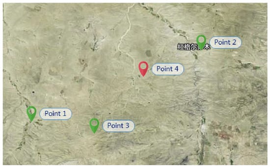
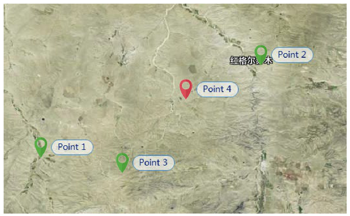
The data used in this research come from an actual PV power station located in north China. The data include PV power data, NWP data, and observed meteorological data. The time range of the data is from May 1, 2023, to August 31, 2024, with a time resolution of 15 min. There are three PV power stations surrounding the target PV station. NWP data for these four PV stations are provided by the same manufacturer. The target PV station is located at Point 4, and the specific distribution is shown in Figure 6.

Figure 6. Geographical location information of PV power stations and NWP points.

3.2. Experimental Design

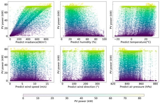
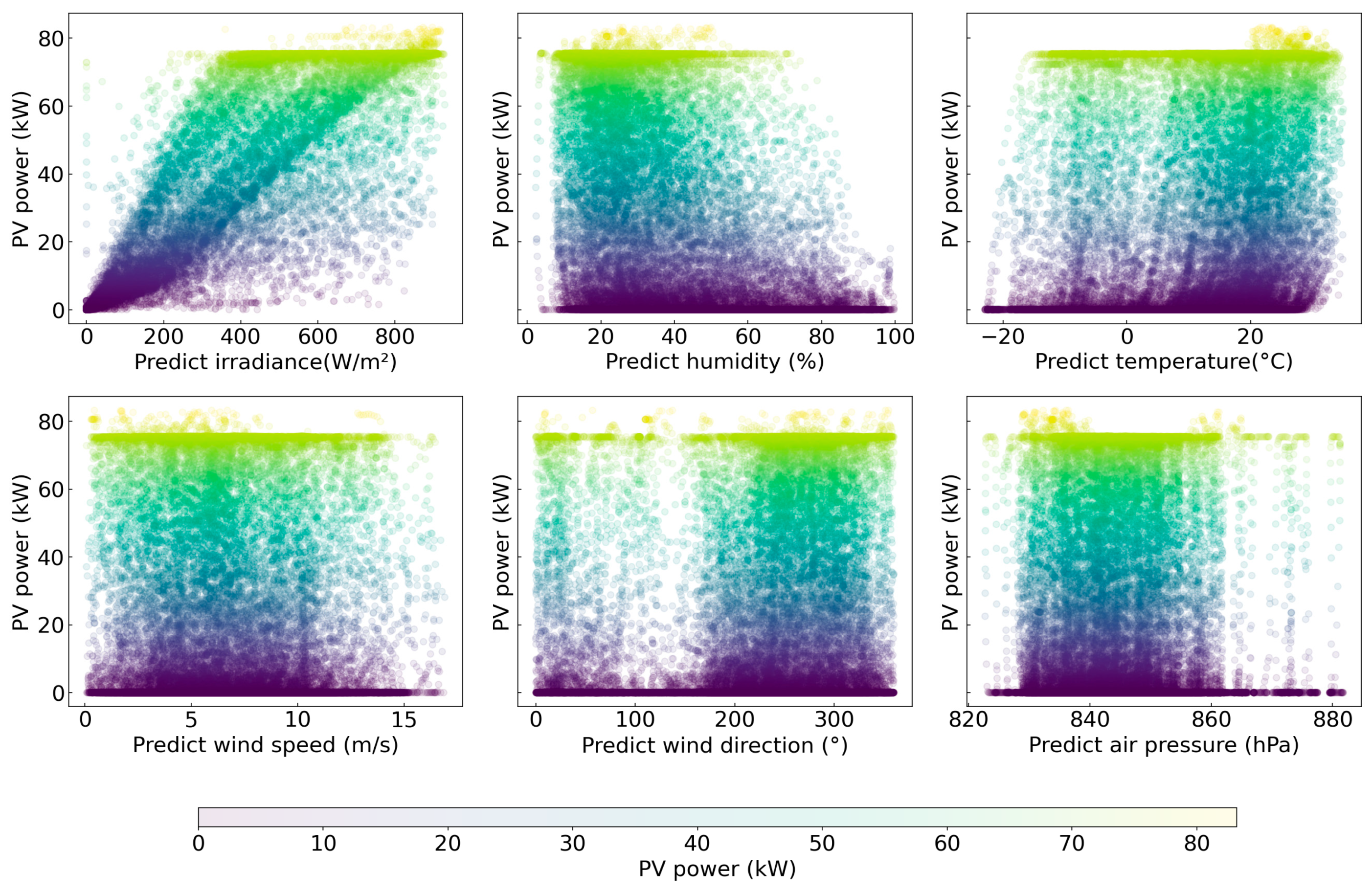
The entire dataset is divided into three parts: the training set (from 1 May 2023 to 31 May 2024), the validation set (from 1 June 2024 to 30 June 2024), and the test set (from 1 July 2024 to 31 August 2024). All data have been normalized. The scatter plots of the predicted meteorological data and PV power data at position 4 are shown in Figure 7.

Figure 7. Relationship between meteorological data and PV power data at position 4.

All the models constructed in this paper were implemented on a Windows 11 operating system with a GeForce RTX 4090 GPU. The programming language used was Python 3.9, with Spyder as the integrated development environment (IDE). The libraries and toolkits employed include PyTorch 2.0.1, Numpy 1.24.3, Pandas 2.0.3, Matplotlib 3.7.2, and others.

This paper uses the Root Mean Square Error (RMSE) and Mean Absolute Error (MAE) as error evaluation metrics for the forecasting results. The mathematical formulas for these error metrics are as follows:

$$RMSE=\sqrt{{\displaystyle \frac{{\displaystyle \sum _{i=1}^n}{(y_i-{\hat{y}}_i)}^2}{n}}}$$

(13)

$$MAE={\displaystyle \frac{{\displaystyle \sum _{i=1}^n}|y_i-{\hat{y}}_i|}{n}}$$

(14)

In the formula, $y$ is the actual value, and $\hat{y}$ is the forecast value. n represents the number of samples.

To evaluate the performance of the proposed model, five benchmark models were selected, as shown in Table 2.

Table 2. Comparison of various models. √ indicates that the feature is extracted, while × indicates that the feature is not extracted.

Method	Model	Model Input	Spatial Features	Temporal Features	Model Settings
Method 1	NGT-former	4-point NWP information	√	√	GCN (24,12) + Transformer (4 layers, 4 heads, 512 embed dim, 512 FFN dim), lr = 1 × 10−4
		Similar-day PV power
		Predicted humidity
Method 2	TCN- Transformer	4-point NWP information	×	√	TCN (3 layers, kernel size = 3, hidden channels = 64) + Transformer (4 layers, 4 heads, 512 embed dim, 512 FFN dim), lr = 1 × 10−4
		Similar-day PV power
		Predicted humidity
Model 3	Transformer	4-point NWP information	×	√	4 layers, 4 heads, 512 embed dim, 512 FFN dim, dropout = 0.5, lr = 1 × 10−4
		Similar-day PV power
		Predicted humidity
Method 4	GCN	4-point NWP information	√	×	3 layers, hidden channels =48, 24 and 12, dropout = 0.5, mean pooling, lr = 1 × 10−3
Method 5	LSTM	4-point NWP information	×	×	3 layers, hidden size =256, 128, dropout = 0.5, lr = 1 × 10−3
		Similar-day PV power
		Predicted humidity
Method 6	BP	4-point NWP information	×	×	hidden layers =3, neurons =256,128 and 64, ReLU, lr = 1 × 10−3

These benchmark models were introduced from different perspectives to examine the respective contributions of spatial modeling and temporal feature extraction in the proposed framework. Specifically, Method 3 (Transformer) was used to verify the contribution of explicit spatial information extraction, since it uses the same multi-point NWP information, similar-day PV power, and predicted humidity as inputs, but does not employ graph-based spatial modeling. Method 4 (GCN) was used to evaluate the contribution of temporal modeling, because it captures spatial correlations among multi-point NWP data but does not model temporal dependencies in historical similar-day power.

In addition, Method 2 (TCN-Transformer) was introduced as a stronger temporal baseline. Compared with the vanilla Transformer, it enhances sequence modeling through temporal convolution and therefore provides a more competitive benchmark to test whether the performance gain of the proposed method comes only from stronger temporal feature extraction. Methods 5 and 6, namely LSTM and BP, were included as representative conventional forecasting models. LSTM is a widely used deep-learning model for time-series forecasting, while BP serves as a shallow neural-network baseline for reference. Through these comparisons, the effectiveness of the proposed framework can be evaluated more comprehensively from the perspectives of spatial modeling capability, temporal modeling capability, and overall forecasting performance.

For a fair comparison, all deep-learning models were trained under the same general training settings. Specifically, the batch size was set to 64 and the maximum number of training epochs was set to 200. Other common training strategies, including optimizer setting and early stopping, were also kept consistent across models unless otherwise specified.

4. Experimental Results

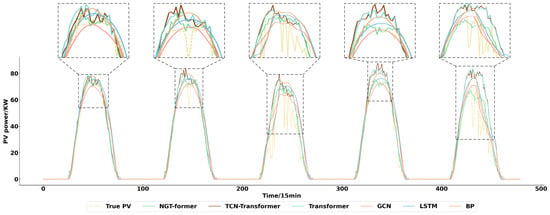
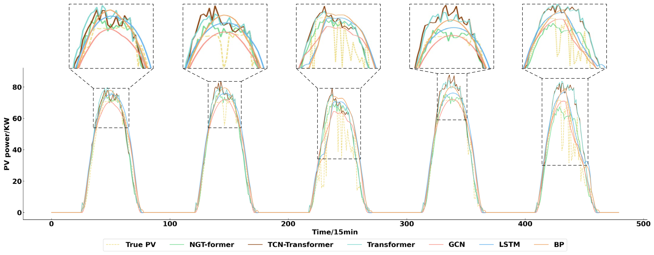
Figure 8 shows the forecasting results of each model over a continuous time period selected from the test set. This segment is presented for qualitative comparison of how different models track the temporal variation in PV power under consecutive operating conditions, while the quantitative evaluation reported in this paper is based on the full test set. The average accuracy of each model is shown in Table 3.

Figure 8. Short-term PV power forecasting results of each model.

Table 3. Comparison of forecasting errors of each model.

Model	RMSE	MAE
NGT-former	0.1115	0.0533
TCN-Transformer	0.1288	0.0593
Transformer	0.1339	0.0619
GCN	0.1409	0.0794
LSTM	0.1666	0.0966
BP	0.1695	0.1015

The experimental results show that the proposed NGT-former achieved the lowest RMSE and MAE among all compared models. Specifically, its RMSE is 13.43%, 16.73%, 20.87%, 33.07%, and 34.22% lower than those of TCN-Transformer, Transformer, GCN, LSTM, and BP, respectively, while the MAE shows a similar trend. This superior performance can be attributed to the joint modeling of spatial and temporal information. Through the GCN module, NGT-former explicitly captures the local spatial correlations among multi-point predicted irradiance series, which helps reduce the uncertainty associated with meteorological inputs. At the same time, by introducing historical similar-day power and the Transformer-based temporal fusion module, the model is able to extract long-range temporal dependencies and integrate heterogeneous inputs more effectively.

Among the benchmark models, TCN-Transformer achieves the second-best performance, indicating that enhanced temporal feature extraction can improve PV forecasting accuracy. However, it still does not explicitly model the spatial relationships among adjacent NWP points. The original Transformer also uses predicted irradiance from four NWP points, but these inputs are directly concatenated along the feature dimension and fed into the model without explicit graph-based spatial representation. As a result, although it can utilize multi-point meteorological information, it cannot fully capture the structured spatial dependencies among adjacent prediction points. In contrast, GCN captures spatial correlations among multi-point irradiance data, but it does not model temporal dependencies in historical power sequences, making it more sensitive to irradiance prediction errors. LSTM has weaker long-sequence modeling capability than Transformer-based models, resulting in relatively lower accuracy. BP, which only learns a direct nonlinear mapping between inputs and outputs, performs worst because of its limited representation ability.

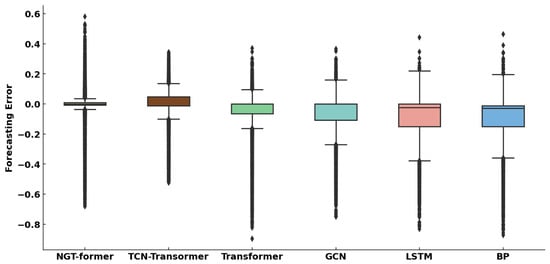
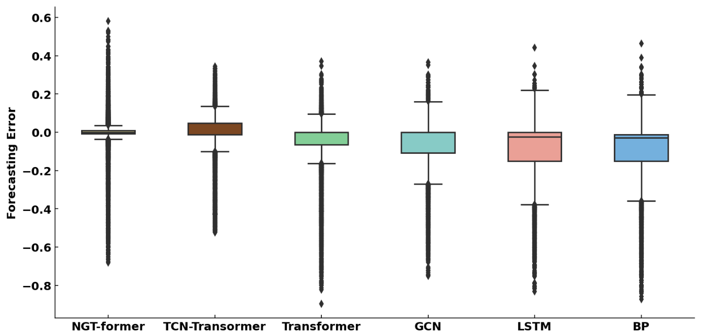
We use a box plot to show the distribution of forecasting errors for different models. From Figure 9, it can be observed that the NGT-former model has the lowest median error and a more concentrated overall error distribution, although outliers are still present. This indicates that the proposed model achieves better overall accuracy and stability than the compared methods on the dataset studied. By contrast, the error distributions of TCN-Transformer, Transformer, GCN, LSTM, and BP are generally more dispersed, with higher median errors and wider error ranges. These results suggest that models without joint spatial–temporal modeling are less effective in capturing the complex variation characteristics of PV power. Overall, the results in Figure 9 further support that integrating graph-structured multi-point NWP information with historical similar-day power helps improve the accuracy and robustness of short-term PV power forecasting.

Figure 9. Forecasting error distribution of each model.

5. Discussion

5.1. Performance Analysis of Models Under Different Weather Conditions

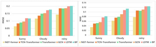
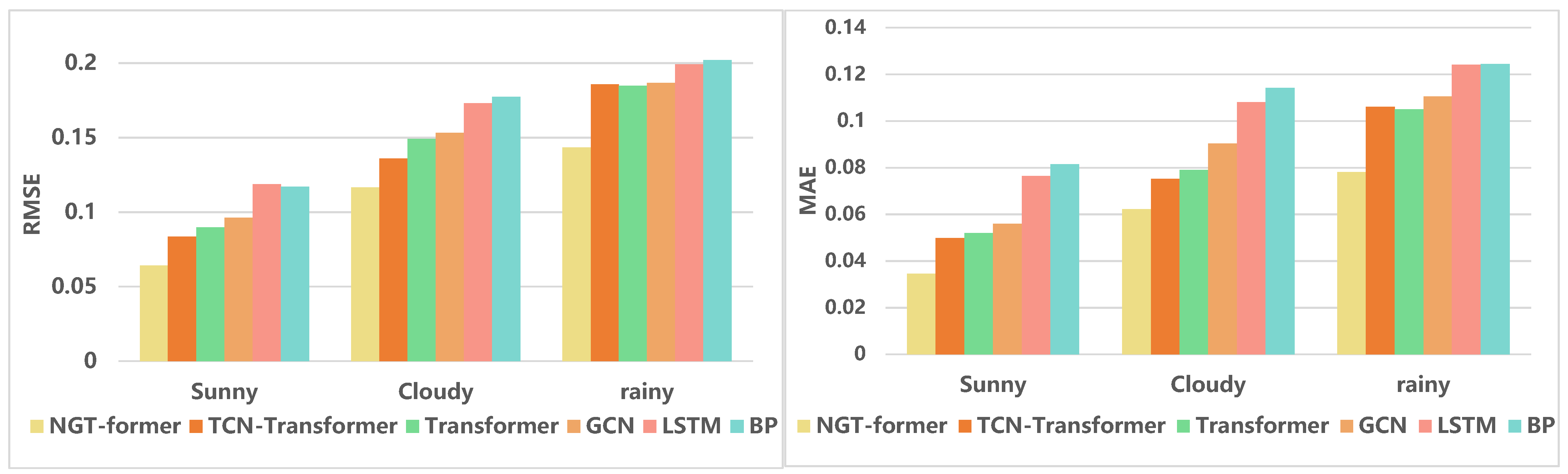
To further analyze the model performance under different weather conditions, the days in the test set were first classified into three weather types, namely sunny, cloudy, and rainy. The weather-type classification was carried out following the method reported in [35], which proposed a weather-state pattern recognition model for short-term PV power forecasting based on solar irradiance feature extraction and support vector machine (SVM) classification. Based on this classification, Table 4 reports the average forecasting errors of the compared models under the three weather types, and Figure 10 presents the corresponding error comparison.

Table 4. Comparison of the RMSE/MAE of each model under sunny, cloudy, and rainy conditions.

Model	RMSE			MAE
	Sunny	Cloudy	Rainy	Sunny	Cloudy	Rainy
NGT-former	0.06427	0.11651	0.14335	0.03460	0.0623	0.0781
TCN-Transformer	0.08351	0.13584	0.18578	0.04991	0.07524	0.10612
Transformer	0.08985	0.14909	0.18490	0.05202	0.07917	0.10506
GCN	0.09623	0.15330	0.18666	0.05595	0.09033	0.11055
LSTM	0.11885	0.17317	0.19902	0.07651	0.10811	0.12409
BP	0.11700	0.17729	0.20206	0.08159	0.11416	0.12452

Figure 10. Comparison of the forecasting errors of each model under different weather conditions.

It can be observed that NGT-former consistently achieves the lowest RMSE and MAE across all three weather types. Under sunny conditions, the forecasting errors of all models are relatively small because the irradiance profile is smoother and more regular. Even in this case, NGT-former still performs best, followed by TCN-Transformer and Transformer. Under cloudy and rainy conditions, however, the errors of all models increase due to stronger irradiance fluctuations and higher meteorological uncertainty. Compared with the benchmark models, the performance advantage of NGT-former becomes more evident in these more complex scenarios. This suggests that explicitly modeling the spatial correlations among adjacent NWP points, together with temporal fusion of historical similar-day power and forecast-related inputs, is beneficial for improving short-term PV forecasting accuracy under variable weather conditions. In general, the proposed model shows not only high accuracy under stable weather conditions, but also stronger robustness under cloudy and rainy conditions than the compared methods.

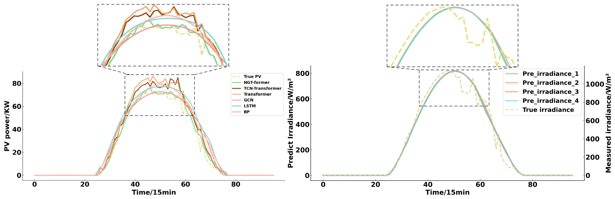
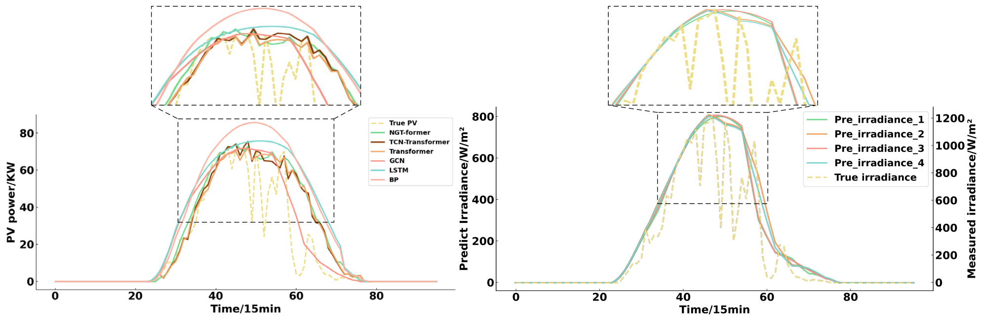
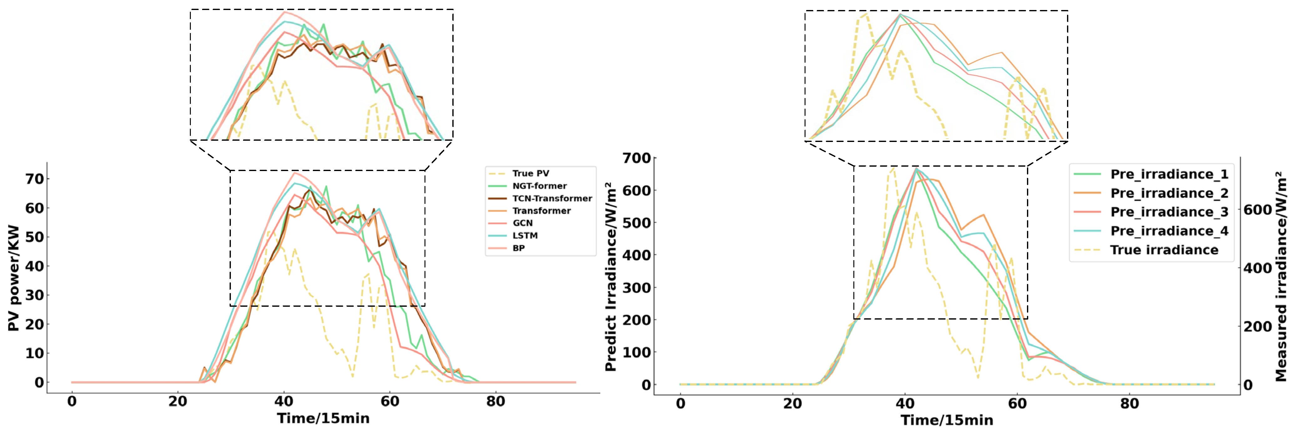
To further analyze the forecasting results of each model under different weather types, we present the specific forecasting results of each model on certain dates under sunny, cloudy, and rainy weather conditions. By combining the predicted irradiance data from four locations and the measured irradiance data from the target PV station, we discuss the performance of each model. The RMSE for each model on specific dates is shown in Table 5.

Table 5. RMSE of each model on the three days listed.

Model	Sunny	Cloudy	Rainy
NGT-former	0.03881	0.12270	0.17503
TCN-Transformer	0.05524	0.14658	0.21365
Transformer	0.06034	0.15867	0.22005
GCN	0.07953	0.16367	0.19848
LSTM	0.07287	0.21497	0.23337
BP	0.06997	0.22856	0.23130

As shown in Figure 11, under sunny weather conditions, the predicted irradiance series from the four NWP points is relatively smooth and stable, with no significant fluctuations. For Transformer, TCN-Transformer, LSTM, and BP, the predicted irradiance from the four NWP points is used as input through direct feature concatenation. As a result, the forecasting curves of these models generally follow the overall shape of the irradiance sequence. Among them, TCN-Transformer and Transformer perform better than LSTM and BP, indicating that stronger temporal modeling is beneficial for capturing the regular variation in PV power under relatively stable weather conditions. In particular, TCN-Transformer achieves better accuracy than the vanilla Transformer, suggesting that temporal convolution helps improve the extraction of local temporal patterns. However, since these models do not explicitly represent the spatial relationships among adjacent NWP points, their ability to utilize multi-point meteorological information remains limited. By contrast, the GCN model explicitly models the correlations among the four NWP points through graph construction, which helps improve the representation of spatial meteorological dependence. Nevertheless, because the GCN in this study does not explicitly model long-range temporal dependence in historical power data, its forecasting curve remains relatively smooth and still fails to capture some local variations in the actual PV power sequence. The proposed NGT-former further combines graph-based spatial feature extraction with Transformer-based temporal fusion. Therefore, it can make better use of both multi-point meteorological interactions and temporal information from historical similar-day power, leading to forecasting results that are closer to the actual power curve and better overall accuracy.

Figure 11. Forecasting results for a certain day under sunny weather.

As shown in Figure 12 and Figure 13, similar patterns can also be observed under cloudy and rainy conditions. When weather changes become more complex and the irradiance sequence alone cannot fully reflect the resulting PV power fluctuations, the limitation of models without joint spatial–temporal modeling becomes more evident. In these cases, NGT-former still provides predictions that are closer to the actual power variations, while TCN-Transformer and Transformer remain better than LSTM and BP, but are still less capable than the proposed model in describing the changing details of the PV power curve.

Figure 12. Forecasting results for a certain day under cloudy weather.

Figure 13. Forecasting results for a certain day under rainy weather.

5.2. Performance Comparison of Various Models at Different Time Scales

This research also compares the distribution of forecasting errors of each model under different forecasting time scales by calculating the daily RMSE for each method. Figure 14 presents the violin plots of the forecasting errors for each model.

Figure 14. Distribution of forecasting errors of each model at different forecasting time scales.

The results show that forecasting accuracy decreases for all models as the forecasting horizon becomes longer, although the extent of degradation differs across models. In comparison, NGT-former, TCN-Transformer, and Transformer exhibit a relatively smaller decline in accuracy, whereas GCN, LSTM, and BP show a more pronounced deterioration. This difference can be attributed to the stronger capability of Transformer-based architectures to capture long-range temporal dependencies, which has been widely reported in previous studies on time-series forecasting and PV power prediction [36,37].

By contrast, the GCN model relies mainly on predicted irradiance as input and does not explicitly model temporal dependencies in historical power data. As the forecasting horizon increases, the uncertainty of meteorological prediction generally accumulates, especially under rapidly changing weather conditions, which may further propagate into PV power forecasting and lead to larger forecasting errors [14,38]. This helps explain why the GCN model shows larger forecasting errors at 32 h and 48 h horizons. LSTM and BP also perform less favorably at longer horizons, partly because of their more limited ability to extract informative features from heterogeneous inputs and to model complex long-term dependencies.

Although NGT-former also uses multi-point NWP inputs, it further combines graph-based spatial features with historical similar-day power for temporal fusion. Existing studies have shown that the joint modeling of spatial and temporal dependencies is beneficial for renewable energy forecasting, because it allows both regional meteorological variation and temporal evolution patterns to be better represented [21,36]. Therefore, the improved performance of NGT-former at longer forecasting horizons can be understood as the result of jointly exploiting spatial correlations among adjacent NWP points and temporal information contained in historical similar-day power. Overall, the proposed method shows a clear advantage in modeling long-term temporal dependence and maintains better forecasting performance in most cases, although accuracy still decreases under some extreme weather scenarios.

5.3. Performance Comparison of Different Models Under Varying NWP Quantities

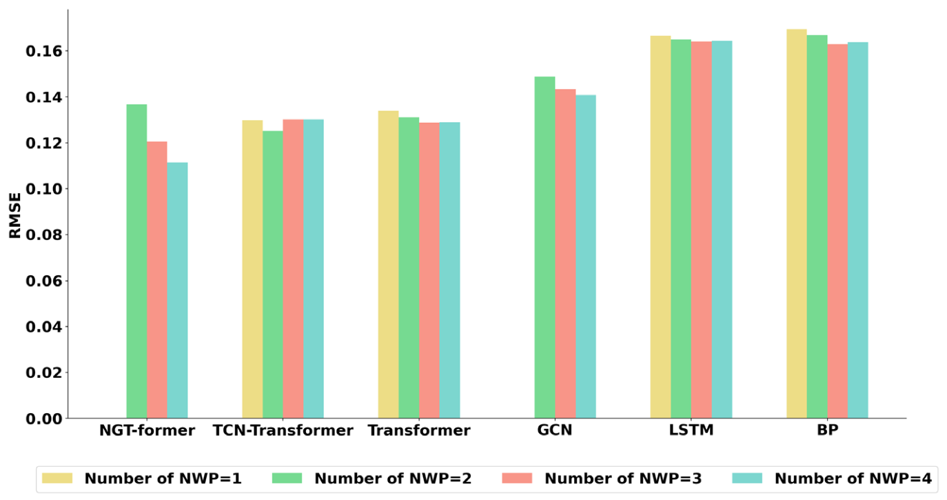
To more objectively evaluate the impact of variations in the number of NWP inputs on model forecasting performance, multiple different location combinations were constructed for each NWP input quantity, and the average forecasting error across these combinations was used as the evaluation result of model performance under that NWP input quantity, as shown in Figure 15.

Figure 15. Comparison of prediction errors across models with different NWP quantities.

Since NGT-former and GCN cannot operate with a single node, results for these two models are not included when the NWP quantity is set to 1. Experimental results demonstrate that the forecasting errors of NGT-former and GCN significantly decrease with an increase in the number of NWP inputs. This is because the growing number of NWP inputs allows the GCN module to construct richer graph information, enabling the model to represent and exploit spatial correlations among multiple input points more effectively, as also reported in previous graph-based forecasting studies [39,40].

By contrast, the effects of increasing the number of NWP inputs on TCN-Transformer, Transformer, LSTM, and BP are relatively limited and less consistent. For these models, multi-point NWP information is mainly introduced through direct feature concatenation rather than explicit spatial modeling. As a result, increasing the number of NWP inputs can provide additional meteorological information, but the performance gain is generally smaller than that of graph-based models. In particular, Transformer shows a gradual improvement as more NWP inputs are included, whereas TCN-Transformer achieves its best performance at an intermediate NWP quantity and then remains relatively stable. For LSTM and BP, the forecasting error decreases only slightly as the number of NWP inputs increases, and the improvement becomes marginal when the NWP quantity reaches 4.

Overall, these results suggest that simply increasing the number of NWP inputs does not necessarily lead to substantial performance improvement for models without explicit spatial representation. In contrast, graph-based models such as NGT-former and GCN can make more effective use of additional NWP points by modeling the spatial correlations among them, thereby obtaining more significant accuracy gains.

5.4. Generalization Test of the Proposed Model

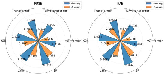
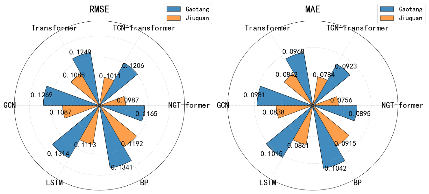
To further evaluate the performance of the proposed model on other PV stations, additional validation was conducted using PV plants located in Gaotang, Shandong Province, and Jiuquan, Gansu Province. For the Gaotang case, three neighboring PV stations were available around the target station. However, the NWP data for these four stations were provided by different vendors. The common data period shared by the four stations in this region was from 1 January 2024 to 31 May 2025, with a temporal resolution of 15 min. For the Jiuquan case, two neighboring PV stations were available around the target station, and the NWP data were also obtained from different vendors. The common data period in this region was from 1 June 2024 to 31 December 2024, with a temporal resolution of 15 min. For both cases, all available data were divided into training and test sets at a ratio of 8:2. Methods 1–6 were then applied to perform short-term PV power forecasting for the two target stations, and the corresponding forecasting errors are presented in Figure 16.

Figure 16. Comparison of RMSE and MAE of different models at the Gaotang and Jiuquan PV stations.

It can be observed that NGT-former achieves the lowest RMSE and MAE in both regions, indicating that the proposed method maintains its performance advantage at additional stations outside the main study case. TCN-Transformer ranks second in most cases, while Transformer, GCN, LSTM, and BP show relatively larger errors. In particular, although the NWP data in these two regions are obtained from different vendors, the proposed model still performs consistently well, suggesting that the graph-based modeling of multi-point NWP information and the fusion of similar-day power provide certain cross-station applicability. Overall, these results further support the effectiveness and generalization capability of the proposed framework for short-term PV power forecasting.

6. Conclusions and Outlook

In this work, we propose a short-term PV power forecasting method based on multi-source NWP data and a GCN-Transformer model. First, we construct a graph network using the geographical information and correlation between the predicted irradiance data from four locations near the target PV station, employing GCN to fully extract spatial features between NWP nodes. Then, we extract the historical similar-day power based on the correlation between the predicted irradiance of the predicted day and that of historical days. Next, the Transformer model is used to fuse the NWP feature vectors, historical similar-day power, and predicted humidity data to forecast the PV power for the target day. Experimental results on the main case study show that the proposed NGT-former achieved lower forecasting errors than the compared benchmark models. In addition, comparative analyses under different weather conditions and forecasting horizons, together with the discussion of the number of NWP inputs and the additional validation results on external PV stations, further demonstrate the effectiveness and robustness of the proposed framework.

The findings of this study are meaningful for practical PV forecasting applications. By combining multi-point NWP information with historical similar-day power, the proposed framework improves the representation of both local meteorological variations and realistic generation patterns. This is beneficial for enhancing day-ahead PV forecasting accuracy and can provide useful support for power system scheduling, reserve arrangement, and market operation.

Despite this, the model proposed in this paper still has room for improvement in terms of accurate short-term PV power forecasting. First, future studies may further explore the intrinsic relationships among the number of NWP points, their geographical distribution, and their spatiotemporal correlations, so as to better understand the role of multi-point NWP information in PV power forecasting. Second, more expressive spatiotemporal graph representations may be developed, and historical similar-day power may be more deeply integrated with graph-based modeling. Third, the current NGT-former uses only predicted irradiance as the input of the GCN module, while predicted humidity, historical similar-day power, and GCN-extracted features are fused in the Transformer module. In future work, additional heterogeneous information may be introduced to capture longer-range dependencies in both graph node features and temporal sequences, although the associated computational cost should also be considered.

References

- IEA. Renewables 2025; IEA: Paris, France, 2025; Available online: https://www.iea.org/reports/renewables-2025 (accessed on 18 September 2025).
- Zhan, Y.; Wang, X.; Xu, Y.; Li, W. A hybrid TCN-LSTM-attention framework for multi-scenario short-term photovoltaic power forecasting incorporating physics-informed neural network strategy. Energy 2026, 344, 139968. [Google Scholar]
- Lari, A.; Sanfilippo, A.; Bachour, D.; Perez-Astudillo, D. Using machine learning algorithms to forecast solar energy power output. Electronics 2025, 14, 866. [Google Scholar] [CrossRef] [Scilit]
- Liu, H.; Du, C.; Guo, R.; Luo, Y.; Cui, Y.; Zi, J.; He, L.; Cao, Y. Short-term PV power forecasting with temporal-attention lstm and successive-halving hyperparameter search. Electronics 2026, 15, 1019. [Google Scholar]
- Lv, C.; Fan, H.; Zhang, Z.; Fan, M.; Run, W.; Yang, L.; Yang, Y.; Liu, D. Ultra-short-term power prediction for distributed photovoltaics based on time-series LLMs. Electronics 2025, 14, 4519. [Google Scholar] [CrossRef] [Scilit]
- Yang, K.; Jiang, C.; Min, Y. Multi-step short-term forecasting of photovoltaic power utilizing autoformer with prophet. Electronics 2026, 15, 1370. [Google Scholar]
- Chen, Y.; Li, X.; Zhao, S. A novel photovoltaic power prediction method based on a long short-term memory network optimized by an improved sparrow search algorithm. Electronics 2024, 13, 993. [Google Scholar] [CrossRef] [Scilit]
- Aravena-Cifuentes, A.; Nuñez-Gonzalez, J.; Graña, M.; Altamiranda, J. Comparative analysis of traditional statistical models and deep learning architectures for photovoltaic energy forecasting using meteorological data. Electronics 2025, 14, 4263. [Google Scholar] [CrossRef] [Scilit]
- Eseye, A.; Zhang, J.; Zheng, D. Short-term photovoltaic solar power forecasting using a hybrid Wavelet-PSO SVM model based on SCADA and meteorological information. Renew. Energy 2018, 118, 357–367. [Google Scholar]
- Böök, H.; Lindfors, A. Site-Specific Adjustment Of A nwp-based photovoltaic production forecast. Sol. Energy 2020, 211, 779–788. [Google Scholar]
- Hu, Z.; Gao, Y.; Ji, S.; Mae, M.; Imaizumi, T. Improved multistep ahead photovoltaic power prediction model based on LSTM and self-attention with weather forecast data. Appl. Energy 2024, 359, 122709. [Google Scholar] [CrossRef] [Scilit]
- Yin, W.; Han, Y.; Zhou, H.; Ma, M.; Li, L.; Zhu, H. A novel noniterative correction method for short-term photovoltaic power forecasting. Renew. Energy 2020, 159, 23–32. [Google Scholar] [CrossRef] [Scilit]
- Dou, W.; Wang, K.; Shan, S.; Zhang, K.; Wei, H.; Sreeram, V. A hybrid correction framework using disentangled seasonal-trend representations and MoE for NWP solar irradiance forecast. Appl. Energy 2025, 397, 126295. [Google Scholar] [CrossRef] [Scilit]
- Dou, W.; Wang, K.; Shan, S.; Li, C.; Zhang, K.; Wei, H.; Sreeram, V. A correction framework for day-ahead NWP solar irradiance forecast based on sparsely activated multivariate-shapelets information aggregation. Renew. Energy 2025, 244, 122638. [Google Scholar] [CrossRef] [Scilit]
- Wu, Y.; Su, P.; Wu, T.; Hong, J.; Hassan, M. Probabilistic wind-power forecasting using weather ensemble models. IEEE Trans. Ind. Appl. 2018, 54, 5609–5620. [Google Scholar] [CrossRef] [Scilit]
- Taylor, J.; Mcsharry, P.; Buizza, R. Wind power density forecasting using ensemble predictions and time series models. IEEE Trans. Energy Convers. 2009, 24, 775–782. [Google Scholar] [CrossRef] [Scilit]
- Chen, G.; Shan, J.; Li, D.; Wang, C.; Li, C.; Zhou, Z. Research on wind power prediction method based on convolutional neural network and genetic algorithm. In Proceedings of the 2019 IEEE Innovative Smart Grid Technologies- Asia (ISGT Asia), Chengdu, China, 21–24 May 2019; pp. 3573–3578. [Google Scholar]
- Mayer, M.; Yang, D.; Markovics, D. The complexity and dimensionality of making deterministic photovoltaic power forecasts from ensemble numerical weather prediction. Energy Convers. Manag. 2025, 344, 120303. [Google Scholar] [CrossRef] [Scilit]
- Wang, F.; Chen, P.; Zhen, Z.; Yin, R.; Cao, C.; Zhang, Y.; Duić, N. Dynamic spatiotemporal correlation and hierarchical directed graph structure based ultra-short-term wind farm cluster power forecasting method. Appl. Energy 2022, 323, 119579. [Google Scholar] [CrossRef] [Scilit]
- Zhen, H.; Niu, D.; Wang, K.; Shi, Y.; Ji, Z.; Xu, X. Photovoltaic power forecasting based on GA improved bi-LSTM in microgrid without meteorological information. Energy 2021, 231, 120908. [Google Scholar] [CrossRef] [Scilit]
- Zhang, M.; Zhen, Z.; Liu, N.; Zhao, H.; Sun, Y.; Feng, C. Optimal graph structure based short-term solar PV power forecasting method considering surrounding spatio-temporal correlations. IEEE Trans. Ind. Appl. 2022, 59, 345–357. [Google Scholar] [CrossRef] [Scilit]
- Simeunović, J.; Schubnel, B.; Alet, P.; Carrillo, R. Spatiotemporal graph neural networks for multi-site PV power forecasting. IEEE Trans. Sustain. Energy 2022, 13, 1210–1220. [Google Scholar] [CrossRef] [Scilit]
- Yang, G.; Xiao, J.; Zhang, C.; Yang, D.; Li, C. A real-time photovoltaic power estimation framework based on multi-scale spatio-temporal graph fusion. Electronics 2025, 14, 4492. [Google Scholar] [CrossRef] [Scilit]
- Jiao, X.; Li, X.; Lin, D.; Xiao, W. A graph neural network based deep learning predictor for spatio-temporal group solar irradiance forecasting. IEEE Trans. Ind. Inf. 2022, 18, 6142–6149. [Google Scholar] [CrossRef] [Scilit]
- Niu, Z.; Zhong, G.; Yu, H. A review on the attention mechanism of deep learning. Neurocomputing 2021, 452, 48–62. [Google Scholar] [CrossRef] [Scilit]
- Gawusu, S.; Zhang, X. Transformer-based deep learning for multi-horizon global power generation forecasting. Energy Convers. Manag. 2026, 354, 121284. [Google Scholar] [CrossRef] [Scilit]
- Gao, J.; Cao, Q.; Chu, Y.; Zhang, D.; Chen, Y. Enhancing photovoltaic power forecasting with cross-variable linear integrated enhanced transformer. Energy Convers. Manag. 2026, 30, 101720. [Google Scholar] [CrossRef] [Scilit]
- Moon, J. A Multi-step-ahead photovoltaic power forecasting approach using one-dimensional convolutional neural networks and transformer. Electronics 2024, 13, 2007. [Google Scholar] [CrossRef] [Scilit]
- Liu, Y.; Yang, M. Ultra-short-term power forecasting for photovoltaic cluster based on dynamic clustering of photovoltaic stations and optimized Ns-transformer combined model. Energy Rep. 2025, 14, 5656–5684. [Google Scholar]
- Wang, F.; Lu, X.; Mei, S.; Su, Y.; Zhen, Z.; Zou, Z.; Zhang, X.; Yin, R.; Duic, N.; Shafie-khah, M.; et al. A satellite image data based ultra-short-term solar PV power forecasting method considering cloud information from neighboring plant. Energy 2022, 238, 121946. [Google Scholar] [CrossRef] [Scilit]
- Liu, X.; Liu, Y.; Kong, X.; Ma, L.; Besheer, A.; Lee, K. Deep neural network for forecasting of photovoltaic power based on wavelet packet decomposition with similar day analysis. Energy 2023, 271, 126963. [Google Scholar] [CrossRef] [Scilit]
- Hu, W.; Zhang, X.; Zhu, L.; Li, Z. Short-term photovoltaic power prediction based on similar days and improved SOA-DBN model. IEEE Access 2021, 9, 1958–1971. [Google Scholar] [CrossRef] [Scilit]
- Yang, X.; Wang, S.; Peng, Y.; Chen, J.; Meng, L. Short-term photovoltaic power prediction with similar-day integrated by BP-AdaBoost based on the Grey-Markov model. Electr. Power Syst. Res 2023, 215, 108966. [Google Scholar] [CrossRef] [Scilit]
- Wang, J.; Hu, W.; Xuan, L.; He, G.; Zhong, C.; Guo, G. TransPVP: A Transformer-Based Method for Ultra-Short-Term Photovoltaic Power Forecasting. Energies 2024, 17, 4426. [Google Scholar] [CrossRef] [Scilit]
- Wang, F.; Zhen, Z.; Mi, Z.; Sun, H.; Su, S.; Yang, G. Solar irradiance feature extraction and support vector machines based weather status pattern recognition model for short-term photovoltaic power forecasting. Energy Build 2015, 86, 427–438. [Google Scholar] [CrossRef] [Scilit]
- Kim, J.; Obregon, J.; Park, H.; Jung, J. Multi-step photovoltaic power forecasting using transformer and recurrent neural networks. Renew. Sustain. Energy Rev. 2024, 200, 114479. [Google Scholar] [CrossRef] [Scilit]
- Hussan, U.; Wang, H.; Peng, J.; Jiang, H.; Rasheed, H. Transformer-based renewable energy forecasting: A comprehensive review. Renew. Sustain. Energy Rev. 2026, 226, 116356. [Google Scholar] [CrossRef] [Scilit]
- Polasek, T.; Čadík, M. Predicting photovoltaic power production using high-uncertainty weather forecasts. Appl. Energy 2023, 339, 120989. [Google Scholar] [CrossRef] [Scilit]
- Verdone, A.; Panella, M.; De Santis, E.; Rizzi, A. A review of solar and wind energy forecasting: From single-site to multi-site paradigm. Appl. Energy 2025, 392, 126016. [Google Scholar] [CrossRef] [Scilit]
- Yang, Y.; Liu, Y.; Zhang, Y.; Shu, S.; Zheng, J. DEST-GNN: A double-explored spatio-temporal graph neural network for multi-site intra-hour PV power forecasting. Appl. Energy 2025, 378, 124744. [Google Scholar] [CrossRef] [Scilit]
Disclaimer/Publisher’s Note: The statements, opinions and data contained in all publications are solely those of the individual author(s) and contributor(s) and not of MDPI and/or the editor(s). MDPI and/or the editor(s) disclaim responsibility for any injury to people or property resulting from any ideas, methods, instructions or products referred to in the content. |
© 2026 by the authors. Licensee MDPI, Basel, Switzerland. This article is an open access article distributed under the terms and conditions of the Creative Commons Attribution (CC BY) license.