


Abstract
With the shift of oil and gas exploitation to deep seas, the 35 kV high-voltage electric slip ring in Single-Point Mooring (SPM) systems faces critical challenges of insulation failure and thermal failure, threatening operational safety. This study aims to investigate its insulation strength and temperature rise characteristics. A three-dimensional electric field model and a magnetic–thermal coupling model considering the skin effect were established using the finite element method (FEM). Simulations were conducted under four high-voltage configurations and various high-current operating conditions, followed by AC breakdown tests and high-current temperature rise experiments for validation. The results show that the maximum electric field (up to 19.53 kV/mm) concentrates at the inlet polytetrafluoroethylene (PTFE) bushing, which is the insulation weak point. The maximum temperature rise at the center ring can be predicted by a power-law model. Moreover, simulation results agree well with experimental data, confirming the reliability of the computational studies. This work provides a theoretical and experimental basis for the optimal design and safe operation of high-voltage slip rings in offshore SPM systems.
1. Introduction
With the depletion of onshore and shallow-sea oil and gas resources, the development of deep-sea oil and gas has become important to meet the growing global energy demand. Submarine oil and gas resources account for 1/3 of the world’s total oil and gas reserves, and the number of deep-sea and ultra-deep-sea oilfields has exceeded six times that of shallow-sea oilfields, driving the gradual shift of oil and gas exploitation activities toward deep-sea areas and the formation of large-scale oilfield clusters [1]. As a core component of deep-sea oil and gas exploitation systems, Floating Production Storage and Offloading (FPSO) relies on the Single-Point Mooring (SPM) system to achieve reliable power transmission and fluid transfer with subsea facilities. To address the requirements of longer transmission distances and larger processing capacities in deep-sea operations, the SPM system is developing toward high voltage and high power. For instance, 35 kV high-voltage SPM has been widely adopted due to its significant advantage in reducing power loss compared to the traditional 10 kV mode. However, the increase in voltage and power brings prominent challenges, including (1) insulation failure caused by uneven electric field distribution [2] and (2) thermal failure induced by high current load [3], potentially leading to platform shutdowns and huge economic losses. Therefore, investigating the insulation performance and temperature rise characteristics of 35 kV high-voltage slip rings is of great engineering significance for ensuring the safe operation of deep-sea oil and gas exploitation platforms.
Existing studies on the reliability of SPM systems primarily focus on insulation failures caused by defective contact between brushes and collector rings, as well as uneven current distribution in electrical slip rings. For instance, Wang et al. analyzed key parameters such as contact statics and main loop resistance of slip rings and verified the reliability of self-designed slip rings through dynamic and static continuous high-current engineering tests [4]. Feng et al. conducted tests on the contact current distribution of electrical slip rings at different angles and confirmed the uneven current transmission among various contacts [5]. Additionally, our team conducted preliminary simulation on the electric field inside a 35 kV slip ring prototype [6]. However, there remains a research gap in two critical aspects: first, studies on insulation failures induced by uneven electric field distribution in SPM systems are relatively scarce, and the precise location of high-electric field regions have not been fully clarified. Second, research on the temperature distribution inside SPM slip rings and the effects of current load, heat dissipation and ambient environment is still insufficient.
To fill the aforementioned research gaps, this paper conducts a comprehensive computational and experimental analysis on the insulation strength and temperature rise of a 35 kV electric-slip ring prototype for offshore SPM systems. The main work includes three key parts: First, a three-dimensional electric field simulation model of the slip ring is established based on the finite element method (FEM) using COMSOL 5.3 software. Second, a coupled magnetic–thermal simulation model considering the skin effect is developed to analyze the temperature rise characteristics of the slip ring, which is also used to investigate the effects of current load, convective heat transfer coefficient, and ambient temperature on temperature rise. A power-law prediction model for temperature rise is also established via multivariable linear regression. Third, experimental validations, including an AC breakdown test and temperature-rising test, are performed to verify the reliability of the simulation results. The results show good agreement between simulation and experiment, providing a reliable basis for the optimal design and safe operation of 35 kV high-voltage slip rings in SPM systems.
2. Methods of Electric and Thermal Simulation
2.1. Structure of the 35 kV Slip Ring Prototype Device
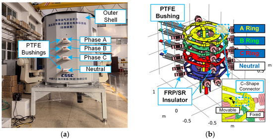
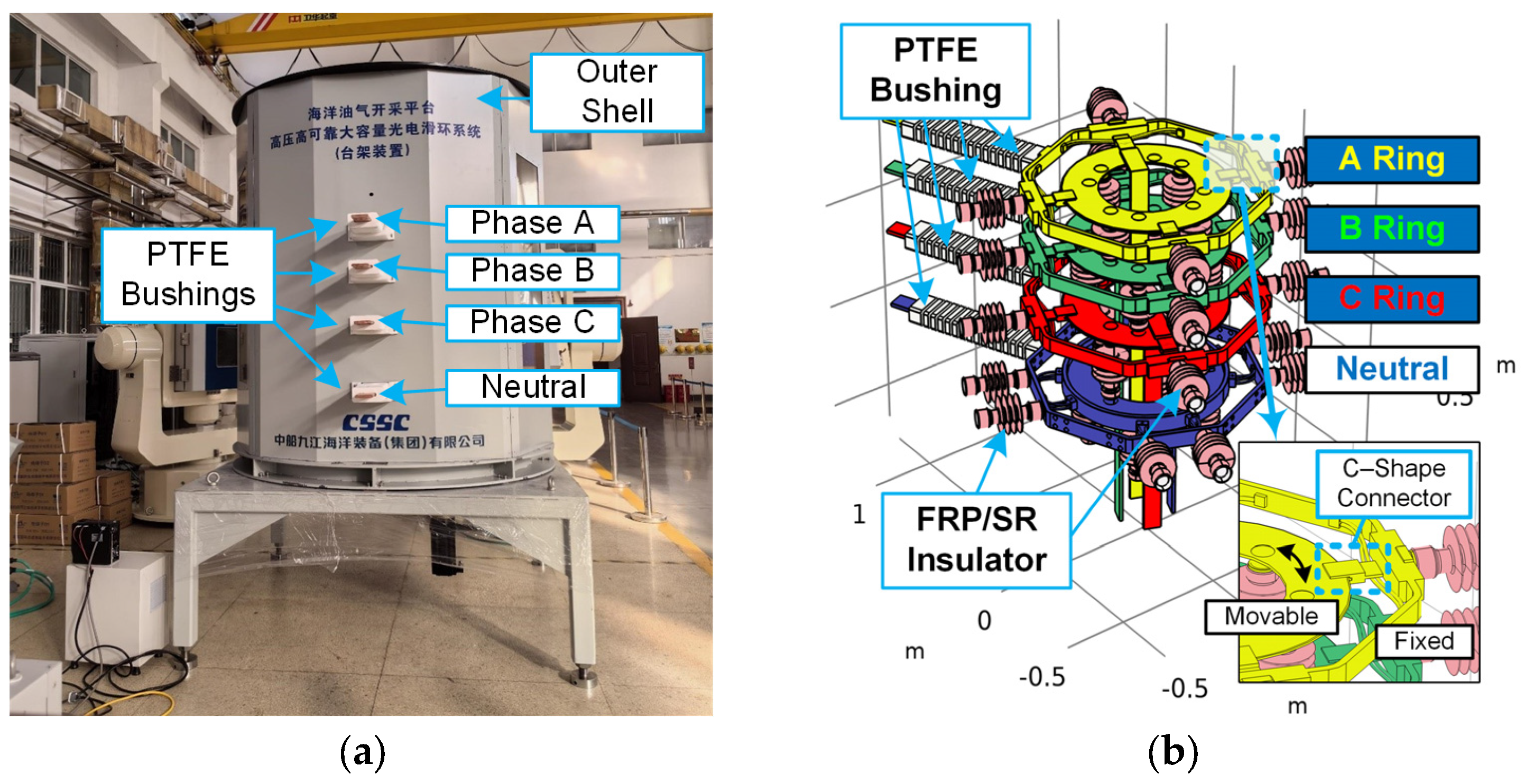
A prototype device of the 35 kV electric slip ring is shown in Figure 1a. With a rated voltage of 35 kV and rated current of 640 A, the device has a polygonal prism structure featuring a circumcircle diameter of 1930 mm and overall height of 2400 mm. Utilizing the three-phase, four-wire AC power configuration, the prototype sequentially integrates four slip rings from top to bottom, i.e., A-phase, B-phase, C-phase, and neutral point. Copper busbars with a cross-sectional area of 80 × 15 mm are installed on both the lateral surfaces and central underside for power input and output.
Figure 1.
Actual device (a) and internal structure (b) of 35 kV electric slip ring.
As shown in Figure 1a, the insulation system employs four PTFE bushings to insulate the horizontal busbar and the outer shell. Moreover, several composite support insulators, consisting of epoxy resin core rods and silicone rubber sheaths, are utilized to isolate different voltages between adjacent slip rings as well as ring grounded electrodes. The interphase spacing between slip rings progressively increases from top to bottom as 180 mm, 240 mm, and 300 mm respectively, while the clearance between slip rings and the grounded enclosure measures 300 mm. As shown in Figure 1b, four C-shape connectors are used in each slip ring as the sliding electrical contact between the fixed outer frame and the rotatable inner rings.
2.2. Calculation Model of Electric Field
2.2.1. Maxwell Equations of Quasi-Static Electric Field
The electric field in a certain domain is determined by the Maxwell equations [7], which can be expressed as follows:
where D is the electric flux density in C/m2, the bold formatting indicates that the variable is a vector, which has both magnitude and spatial direction; B is the magnetic flux density in T; E is the electric field in V/m; H is the magnetic field in A/m; ρ is the electric charge density in C/m3; and J is the electric current density in A/m2.
The relationship between flux/current variables (D, B and J) and field variables (E and H) can be determined by the material equations (i.e., constitutive equations):
where ε0 = 8.854 × 10⁻¹² F/m is the vacuum permittivity of the electric field and εr is the relative permittivity; μ0 = 4π × 10−7 H/m is the vacuum permeability of magnetic field and μr is the relative permeability of insulation materials; and σ is the electric conductivity in S/m.
Since the insulation structure of the slip ring prototype (<2 m) is much smaller than the wavelength of a 50 Hz electromagnetic field (6000 km), the electro-quasi-static (EQS) assumption can be used in the electric field analysis; i.e., the electric curl field induced by the time derivative of the magnetic field can be neglected. Therefore, the Equations in (1) and (2) can be rearranged to the following equations:
Considering that the insulation performance of the slip ring prototype is mainly correlated to the electric field E, and the Helmholtz Theorem indicates that a vector is determined if the curl and divergence of this vector is specified under certain boundary conditions, Equation (3) can be further simplified to determine the quasi-static E field as follows:
In Equation (4), the 3rd line indicates that the curl of the electric field is zero; this implies that the vector-form electric field E is conservative (i.e., irrotational). This means that the electric field is equivalent to the gradient of a scalar-form field. Here, the electric potential V is used as this scalar field, and V and E have the following relationship:
Taking into consideration the 1st and 2nd equations in (4) and Equation (5), the electric potential V in the insulation system of the slip ring prototype can be determined by
It should be noted that the proposed model employs a macroscopic electro-quasi-static approach to solve the Laplacian background field. While space-charge accumulation is a critical micro-mechanism for partial-discharge (PD) inception at gas–solid interfaces, it is not incorporated in this study, as the primary objective is to identify macroscopic geometric weak points and guide structural optimization during the prototype development stage.
2.2.2. Simplification of V-Field Equation Under AC 50 Hz Voltage
Since the slip ring is operated at 50 Hz power frequency, Equation (6) can be transferred into the frequency domain using the Fourier transform, which can be expressed as
where is the phasor of the electric potential, and ω = 100π rad/s is the angular frequency of the 50 Hz sinusoidal voltage waveform. Equation (7) is the Laplace equation of frequency-domain electric potential, considering both the permittivity and conductivity of the dielectric materials.
Although it appears to be complex, this expression can be further simplified based on the properties of insulation materials. As shown in Table 1, the permittivity term (ωε0εr) is 3 to 5 orders of magnitude higher than the conductivity term in the dielectric materials of 50 Hz slip ring prototype. Thus, the contribution of electrical conductivity to the potential distribution can be neglected, and Equation (7) can be transformed to
Table 1.
Comparison between dielectric and conductive properties of electrical insulation material in slip ring prototype.
Considering that ω and ε0 are constant, and the relative permittivity in the problem domain can be varied due to the spatial transition of different insulation materials, Equation (8) can be further simplified to
Obviously, Equation (9) has a similar form to the Laplace equation of the electro-static field, indicating that the electric field distribution under AC 50 Hz voltage excitation can be calculated using the electro-static model.
2.2.3. Boundary Conditions of Electric Field
During the simulation of an electric field, there are mainly two types of boundary conditions, i.e., the potential boundary at the conductor’s surface and the continuity conditions at the dielectric interface. Details of these boundary conditions are described below.
- (1)
- Potential boundary at the conductor’s surface
The potential boundary condition, also known as the Dirichlet boundary condition, is one of the most widely used boundary conditions in electric field simulation. It is defined by specifying the exact electric potential value (V) at every point on a given boundary, including the high-voltage conductors (V ≠ 0) and grounded conductors (V = 0).
- (2)
- Continuity conditions at the dielectric interface
Continuity conditions at the dielectric interface are essential constraints that govern the behavior of electric field quantities across the boundary between two different insulating materials. These conditions are derived from Maxwell’s equations and ensure the physical consistency of the electric field distribution at the interface. There are three core aspects with distinct mathematical expressions:
First, the electric potential is continuous at the interface, meaning there is no abrupt change in potential when crossing from one dielectric to another:
Second, the normal component of the electric-displacement vector () is continuous in the absence of free surface charges, which accounts for the continuity equation at the normal direction of dielectric interfaces:
Third, the tangential component of the electric field strength Et,
is continuous, preventing the accumulation of electric field energy along the interface. Therefore, the tangential continuity equation can be determined as
In high-voltage engineering applications, these conditions are particularly relevant for structures with multiple dielectric materials, such as gas–solid interfaces. Accurately implementing these continuity conditions in finite element models is vital for capturing the electric field distortion at material interfaces, which is a key factor in assessing insulation performance and identifying potential breakdown risks.
2.2.4. FEM Calculation in Electric Field
As described in Section 3.2.1, the electric field of the insulation structure is evaluated according to the calculation results of the electro-static field, which is conducted by the COMSOL software using the finite element method (FEM). The specifications of the FEM calculation are as follows
Geometrical Structure
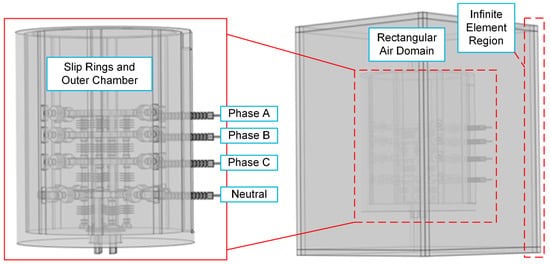
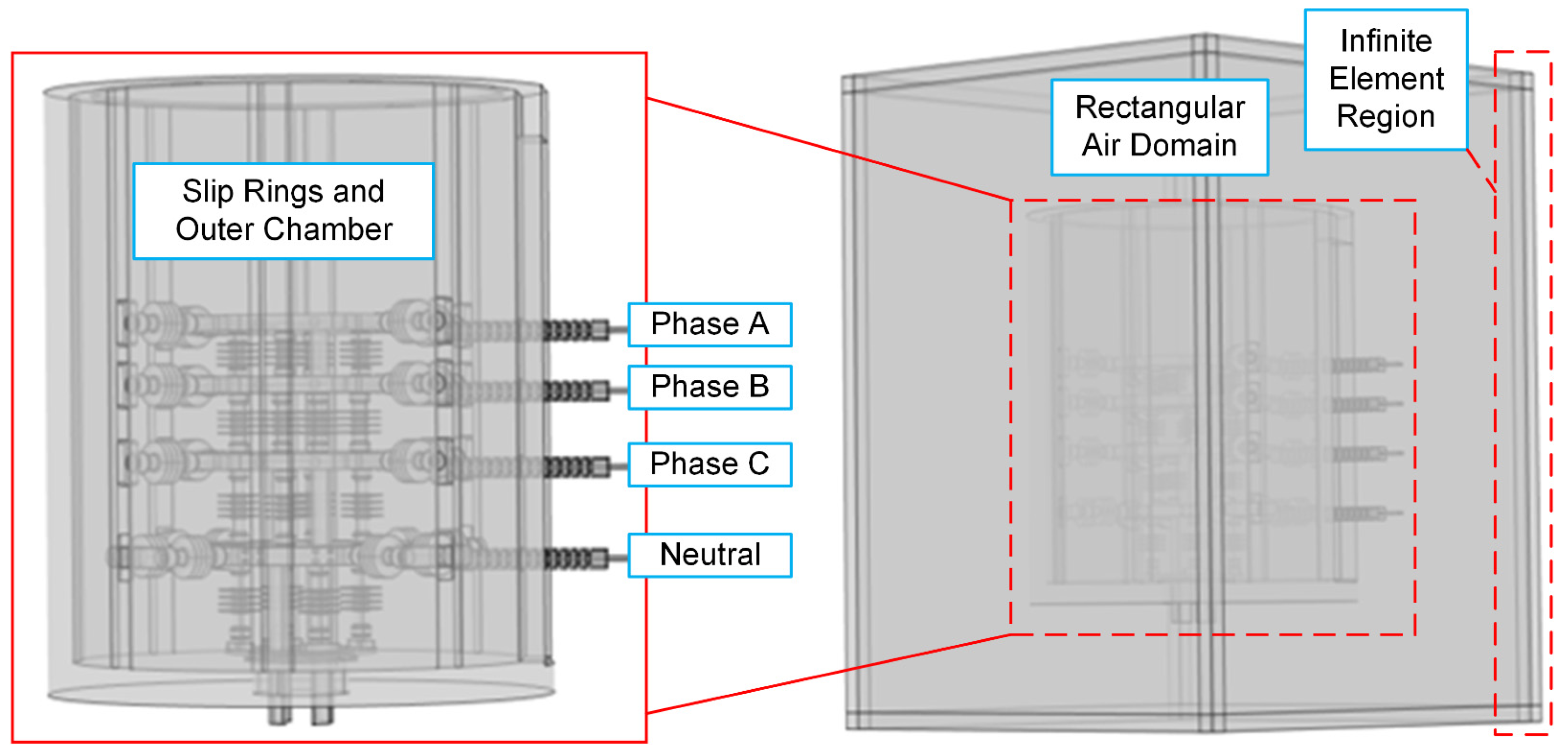
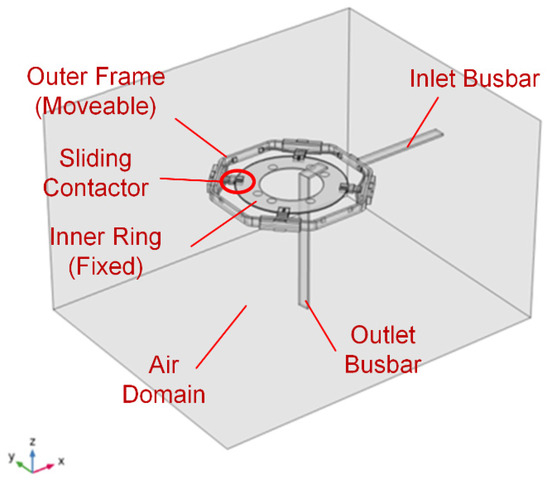
A three-dimensional geometrical structure was constructed using CREO v4 CAD software and converted to STP format. During the model construction process, some tiny structures (connecting bolts, assembly holes, etc.) were removed and the outer shell was simplified to a hollow cylinder. These simplifications do not significantly affect the electric field, but can effectively reduce the memory cost and calculation time. The STP file was then imported to COMSOL software for further calculation, and a rectangular box was built to wrap the slip ring prototype, as illustrated in Figure 2.
Figure 2.
Geometrical model for electric field calculation in COMSOL software.
Another important setting of geometrical structure is the application of an infinite element region on the exterior shell of the rectangular air domain. In COMSOL software, the Neumann boundary condition (named as “Zero Charge” in COMSOL software) is conventionally employed on the exterior boundaries of the calculation region, which sets the normal component of the electric field to 0. This may induce deviation between the actual and simulated values of the electric field and cause calculation errors. Generally, this boundary error is relieved by covering a very large air domain (e.g., 10 times larger than the studied device) on the outer area of calculation, which, however, leads to extremely high computation cost in three-dimensional, large-size problems.
Here, the infinite element technique is used to balance the precision and cost, which adds some rectangular “infinite element regions” outside the exterior boundary. Inside the infinite element region, special basis functions (e.g., exponential decay functions) are used in the FEM to mathematically describe the behavior of the infinite region, avoiding the need to simulate the entire infinite space.
Material Definition
According to Equation (9), the relative permittivity εr of the conducting and dielectric material is required for the calculation of the electric field. The permittivity of the materials used in the COMSOL simulation is listed in Table 2, which is based on the simulation and experimental data in the previous literature. It should be noted that due to the similarity of the epoxy core rod and silicone sheath in the insulator, their permittivity was set to the identical value of 4.0.
Table 2.
Dielectric parameters of electrical insulation material in slip ring prototype.
For the metallic conductors, strict Dirichlet potential boundary conditions were explicitly applied to all exterior surfaces enveloping the conductors. However, considering the extreme multi-scale nature of the 3D CAD model (ranging from a 2.4 m overall height to sub-millimeter local features), manually selecting all continuous surfaces can occasionally miss tiny, hidden internal faces or imperfect Boolean intersections. To address this, an additional numerical “fail-safe” was implemented by setting the relative permittivity of the bulk metal domains to an extremely large value (ϵr = 1.0 × 10⁶). This dual approach mathematically enforces ∇V ≈ 0 within the bulk volume, ensuring the conductors behave as strict equipotential bodies without introducing non-physical field distortions at the dielectric interfaces.
Boundary Conditions (Voltage Application)
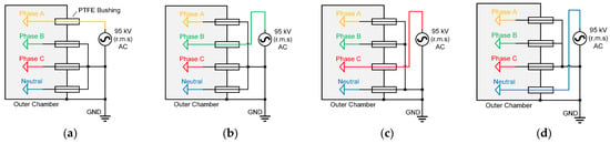
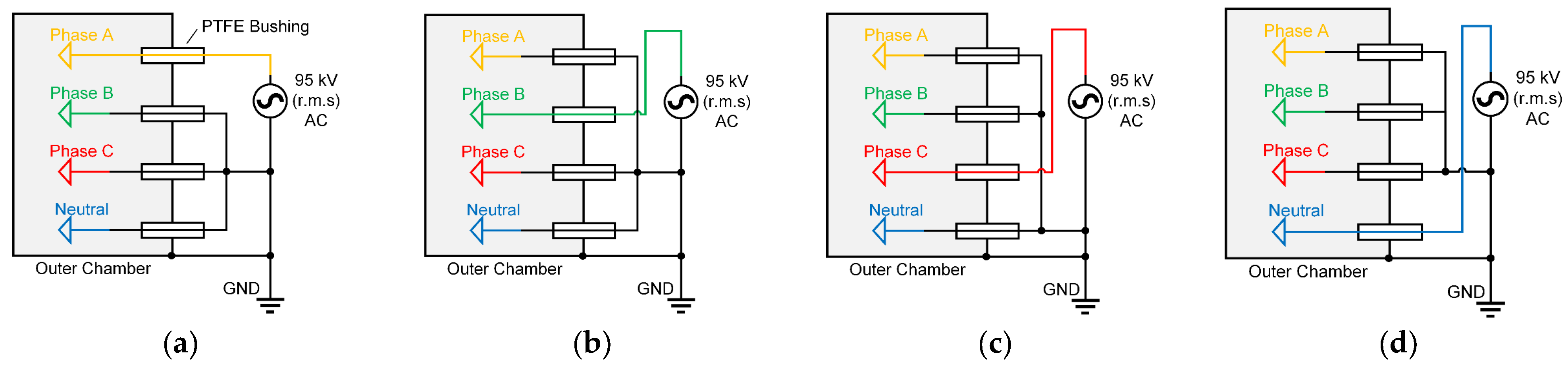
To simulate the electric field distribution, firstly, the Dirichlet boundary condition (i.e., potential value on the conductors) should be determined. According to the standard of high-voltage connecting and switching devices [8], the insulation test of AC high voltage is conducted by applying 95 kV (r.m.s.) high voltage (HV) on one of the metal conductors (phase A, phase B, phase C or neutral conductor N). Since the insulation performance is determined by the peak value (NOT r.m.s.) of the test voltage, the applied potential on the HV conductor is . Despite the HV conductors, other conductors and the outer chamber are grounded (zero potential) during the simulation. Therefore, a total of 4 configurations of HV tests are simulated in this study, as shown in Figure 3.
Figure 3.
Conceptual illustration of high voltage and grounding application in the electrical insulation tests, including the test on (a) phase A, (b) phase B, (c) phase C and (d) neutral conductor.
It should be noted that since the applied peak voltage (134.3 kV) is nearly triple the peak line-to-line voltage during actual 35 kV operation (~49.5 kV), the test environment generates a significantly higher voltage gradient, enabling strict conditions during type tests. Furthermore, given the large interphase spacing (180–300 mm), voltage variations from self- and mutual-induction are negligible. Thus, validating the insulation under these stringent conditions ensures an ample safety margin for actual three-phase field superposition.
FEM Meshing and Solving Method
In the FEM simulation of the electric field, tetrahedral, second-order calculation elements were employed in the domains of the metal conductor, solid insulation and air, and the rectangular, hexahedral elements were utilized in the infinite element regions. A “Finer”-mesh-size configuration is implemented on the whole model in COMSOL, where the tetrahedral element size ranges from a 220 mm maximum to 16 mm minimum. To further increase the calculation accuracy, the “extra-fine”-mesh-size configuration with local refinement was used on the high-field regions, such as the edges of the conductive rings, insulators, and bushings. In these mesh-refined regions, the maximum element size was restricted to within 5 mm, while the minimum size was set to 0.2 mm. The above meshing approach aims to balance computational efficiency and the accuracy of simulation results, which, however, still generate about 40 million FEM elements and are difficult to calculate on PCs. In this study, an FEM workstation (64-core AMD CPU and 256 GB RAM) is utilized, and one round of simulation can be conducted in 1~2 h.
2.3. Calculation Model of Temperature Rise
2.3.1. Heat Source from Ohmic Heating Considering Skin Effect
To calculate the temperature distribution inside the slip ring structure, firstly, the heat source must be assessed. The skin effect describes alternating current (AC) concentrating on a conductor’s surface, with current density decaying exponentially inward. Governed by Maxwell’s equations, it arises from electromagnetic induction and energy loss. When AC flows, it generates a time-varying self-induced magnetic field (Ampère’s law), which induces a closed-loop electric field opposing the original current (Faraday’s and Lenz’s laws), creating eddy currents. Surface eddy currents repel the original current outward, while deeper, weaker eddy currents have a negligible effect. Eddy currents dissipate Joule heat via the conductor’s resistivity, further driving the exponential current decay with depth—critical for calculating slip ring temperature distributions [7].
Quantitatively, the current density J at a depth d from the conductor surface follows the exponential law:
where J0 is the current density at the surface, and δ (skin depth) is the depth at which the current density decreases to 1/e (≈37%) of its surface value. The skin depth is determined by the conductor’s properties and the frequency f of the AC:
where ω = 2πf is the angular frequency of the AC, and μ (magnetic permeability) and σ (electrical conductivity) are material-dependent parameters.
From the above introduction on skin effect, it can be seen that higher frequencies, higher magnetic permeability, or higher electrical conductivity result in a smaller skin depth, intensifying the current concentration on the surface as well as the Joule heating. For instance, the copper conductors used in the slip ring system have a conductivity of σ = 5.8 × 10⁷ S/m and magnetic permeability μ similar to the permeability of vacuum (i.e., μ = μ0 = 4π × 10−7 H/m), and the conductors work under 50 Hz AC, Therefore, the skin depth can be calculated as δ = 9.3 mm, which is at the same order of magnitude of the conductors and indicates that the skin effect of the conductors cannot be neglected.
2.3.2. Heat Transfer Involving Joule Heating and Thermal Conduction
For steady-state heat transfer (where temperature does not change with time), the governing equation is based on the balancing between heat generation and dissipation [9]. Specifically, the volumetric heat generation rate qsrc (W/m3) at any spatial position is always canceled out by the volumetric heat dissipation rate (i.e., the divergence of the heat flux qdis (W/m2), which can be expressed as
As for the heat source qsrc, it is generated from internal sources (e.g., Joule heating of flowing current). Here, the heat source can be calculated by the current density J (considering skin-effect as discussed in Section 2.3.1) and electric conductivity σ using Ohm’s law:
In engineering heat transfer simulations, the core objective is to solve the spatially varying temperature field T (K). Therefore, the dissipated heat flux is not directly solved but computed via the following expression:
where k is the thermal conductivity of the material, W·m−1·K−1. Using the Laplace operator , the PDE expression of heat transfer inside the simulation domain (i.e., copper conductor) in (12) is converted to the following:
2.3.3. Boundary Conditions Involving Convection and Radiation
Boundary conditions define heat exchange between the simulated domain and its surroundings, directly linking to ambient temperatures. This research mainly focuses on the heat transfer at the surface of solid materials, which can be classified into two pathways—convection and radiation.
Convective Heat Transfer
Convective heat transfer is a common heat transfer mode involving fluid (gas/liquid) and solid surfaces, combining fluid macro-motion (natural convection driven by density gradients or forced convection by external forces like fans) and molecular thermal conduction. As for the convection process of the slip ring system, the heat dissipation medium (air) has low density (1.29 kg/m3), large flow space (2 m), low flow speed during natural convection (0.1 m/s) and low viscosity (1.79 × 10⁻⁵ Pa·s). This will lead to a high Reynolds number (~14,400), indicating significant turbulent effect, and increase the computational cost and instability to directly solve the fluid–thermal behavior at the solid–fluid interface. Therefore, we use Newton’s law to simplify the thermal-simulation process, and use a single variable h to characterize the convective outward heat flux qc:
where h is the convective heat transfer coefficient h (W·m−2·K−1), Ts is the temperature at the solid–fluid boundaries, and T∞ is the air’s temperature at infinite distance (usually identical to the ambient temperature).
Considering that at steady state, qc is canceled out by the conductive heat dissipation qdis at the solid-air interface, the convective boundary condition can be written as
In this equation, n is the outward normal vector of the solid material’s surface. Equation (17) determines the Neumann boundary condition of convective cooling using a simple mathematical form, and can be easily realized by FEM simulation packages.
Radiative Heat Transfer
Thermal radiation induced by outward infrared light is another important heat transfer pathway. Based on the gray-body approximation, the radiative outward heat flux qr is given by
This incorporates emissivity εrad (ranges from 0 to 1), the Stefan–Boltzmann constant σrad = 5.67 × 10⁻⁸ W·m−2·K−4, and ambient temperature T∞. Under steady-state, a similar Neumann boundary condition of thermal radiation can be determined as
In summary, the Neumann boundary condition of outward thermal flux can be determined by the combination of equations.
2.3.4. FEM Calculation of Temperature Rise
Geometrical Structure
In general, the original slip ring shown in Figure 2 is difficult to conduct the magnetic–thermal FEM simulation for. Simplification of the simulation model is critical. In this study, the simplification of the SPM model is conducted under the following considerations:
- (1)
- The metal enclosure is excluded from the thermal simulation based on two considerations: First, the enclosure is not part of the active electrical circuit and thus lacks direct Ohmic heating. Second, the section of the enclosure surrounding the high-current busbars is constructed from non-magnetic stainless steel (e.g., 316 L austenitic stainless steel) with low-eddy-current-loss characteristics. This material selection significantly suppresses inductive heating caused by the alternating magnetic fields of the busbars, rendering the enclosure’s heat generation negligible compared to the primary copper conductors.
- (2)
- The thermal conductivity of copper conductor (385~401 W·m−1·K−1) is much higher than polymer insulation (0.2~0.5 W·m−1·K−1). Therefore, the insulators can be neglected during the simulation because the heat dissipation is dominated by convection and radiation from the large exposed copper surfaces. Although insulators provide local thermal resistance at contact regions, the high thermal conductivity of copper ensures efficient internal heat distribution, preventing significant localized temperature pooling. Thus, this simplification has a negligible impact on the predicted peak temperatures and overall steady-state distribution.
- (3)
- The distance between different conductors (240~300 mm) is much larger than the geometrical size of the conductors (15–30 mm). According to the analytical formula [10,11], the proximity effect factor yp for this configuration is less than 2%, suggesting that magnetic coupling between phases has a minimal impact on the overall current density distribution compared to the self-induced skin effect. Therefore, the proximity effect can also be neglected, which means a single conductor can be used to simulate the temperature rise.
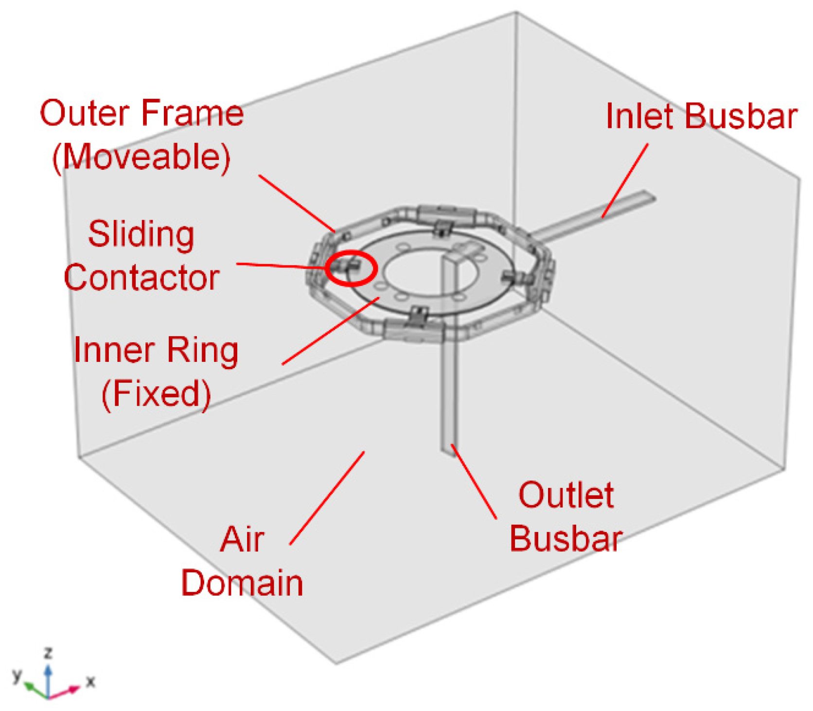
The simplified model shown in Figure 4 contains one of the copper conductors (phase A ring) and a certain range of adjacent air, which reduces the size and complexity of the FEM simulation.
Figure 4.
Structure of the simplified model (i.e., phase A ring) for magnetic–thermal simulation.
Material Definition
There are 2 main materials in the simulation model, air and copper, whose properties are shown in Table 3. Considering the large fluctuations in the operating temperature, the resistance–temperature effect of the copper conductor should be considered. Therefore, the electrical conductivity of the copper material is replaced by the following formula, representing the linear electrical conductivity.
where σ represents the electrical conductivity (S·m−1) of the conductor at temperature T (in Kelvin); ρ0 = 1.72 × 10⁻⁸ Ω·m is the resistivity of the conductor at the reference temperature Tref = 298.15 K (20 °C); and α is the temperature coefficient of resistance, whose typical value for copper conductors is α = 0.0039 K−1.
Table 3.
Material parameters related to thermal simulation in slip ring prototype.
Physical Model and Boundary Conditions
As discussed before, the simulation of the temperature rise in this slip ring device is to calculate the conductor’s temperature under the excitation of a certain current when the heating and cooling processes reach equilibrium. The heat source in this problem comes from the Joule heat, and the main cooling method is air convection and thermal radiation on the surface of the conductor. Due to the self-induction effect under AC, there is a “skin effect” in the conductor, in which the current density concentrates on the conductor’s surface.
From the above viewpoints, this simulation problem can be constructed as a coupled simulation of current and thermal fields. The current field simulation determines the spatial distribution of current density (and thus the resistance value) under a 50 Hz magnetic field. Thermal simulation determines the temperature distribution under Joule heating, convection cooling and infrared radiation. Coupling between current and thermal field is mainly represented by Equation (20), i.e., the temperature dependency of copper resistance.
The aforementioned simulation problem is analyzed using COMSOL software. A 50 Hz AC ranging from 160 A r.m.s to 1120 A r.m.s. flows in through the right port of the inlet busbar and out through the lower port of the outlet busbar in Figure 4. A certain area of the rectangular air domain is set around the conductor to provide a carrier for the simulation of the magnetic field distribution. For the heat dissipation through convective cooling, the heat transfer coefficient h on the surface of the copper conductor is used to replace the direct simulation of turbulent flow, whose effect on temperature rise will be discussed in the following paragraphs. As for the thermal radiation effect, since the conductors are smoothly polished copper, their infrared emissivity εrad is set to 0.05.
FEM Meshing and Problem Solving
For the problem of significant size difference between the overall structure and detailed parts, the locally refined adaptive-mesh-setting method is adopted. Specifically, the overall meshing adopts a “Finer” setting, in which the characteristic size of the tetrahedral mesh dynamically varies between 25 and 200 mm. For refined areas such as the surface of the conductor, the maximum mesh size is reduced to 1 mm to precisely calculate the current density and temperature distribution. The simplified simulation model after the self-adaptive meshing contains about 370,000 tetrahedral elements.
To solve this FEM problem, the generalized conjugate residual with deflated restarting (GCRO-DR) solver is utilized. Specifically, on the simulation workstation (AMD Ryzen 64-core CPU, 256 GB RAM, 16 TB hard drive), a single simulation takes about 12 min, providing an efficient analysis method for the optimization design of slide rings.
3. Calculation Results of Electric Field and Temperature Rise
3.1. Simulation of Electric Field Distribution
The three-dimensional electric field distribution under the power–frequency withstand voltage test (95 kV r.m.s., 134.3 kV peak) was calculated for four configurations: high voltage applied to phase A, phase B, phase C, and the neutral point, respectively, with all other conductors and the enclosure grounded.
3.1.1. Electric Field Distribution Under Excitation of Phase A Ring
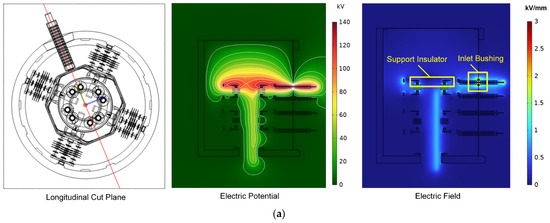
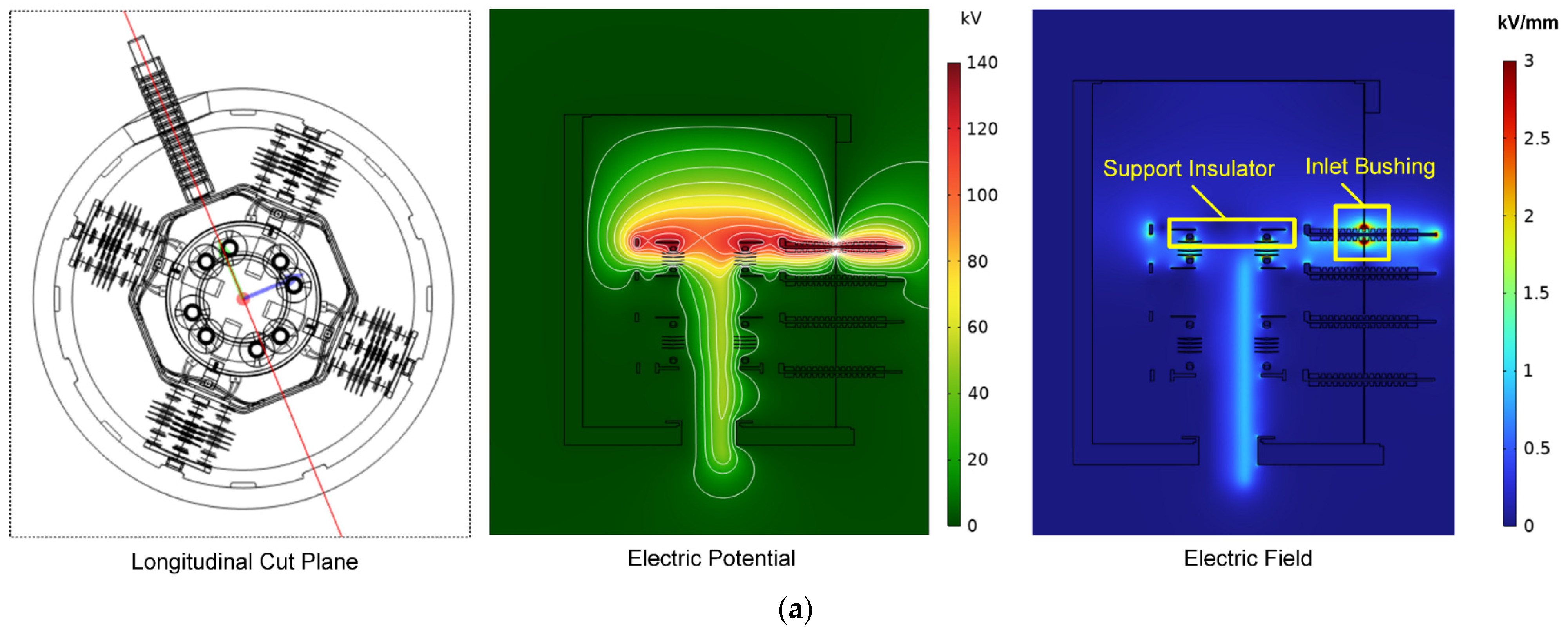
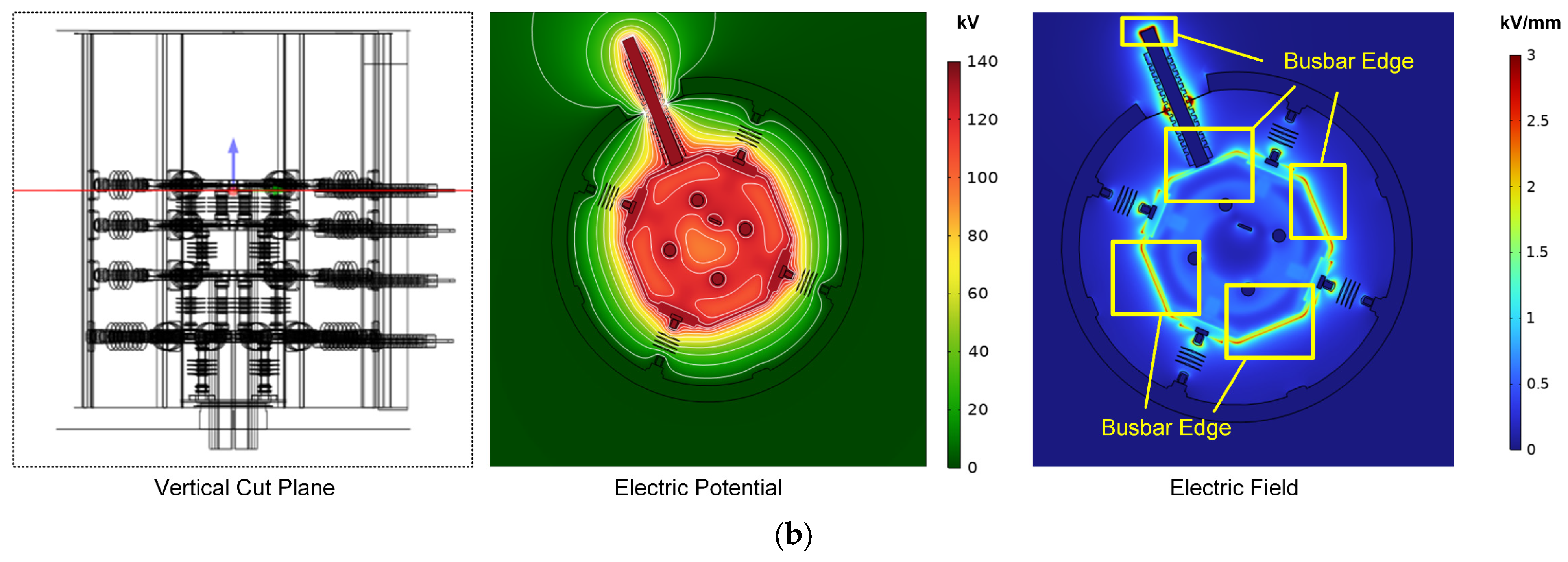
Figure 5 shows the electric potential and field on the cut planes of the phase A ring. It should be noted that the electric field distribution is similar when high voltage is applied to other conductors, which indicates that the situation of phase A excitation can be used as an example. From Figure 5, we can see that when a 95 kV r.m.s. high voltage was applied, the contour lines of the electric field are concentrated at the gap between the inlet busbar and outer shell (grounded to zero potential). This leads to the localized intensification of the electric field to a maximum field strength of 15.7 kV/mm at the bushing outlet. This value significantly exceeds the average breakdown strength of air (~3 kV/mm), and is also close to the breakdown strength of PTFE material (20–30 kV/mm), identifying the bushing outlets as the most vulnerable points for partial discharge or flashover initiation during the test.
Figure 5.
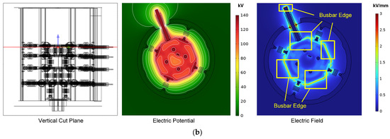
Electric field distribution on phase A cut planes when 95 kV r.m.s high voltage is applied on phase A ring, including (a) longitudinal cut plane and (b) vertical cut plane.
Despite the electric field concentration on the inlet bushing, some other field concentration regions are also observed. One region is the place surrounding the rectangular busbars, particularly at the corner edges of the busbars. Another region is the edges and terminal parts of support insulators, particularly those adjacent to the excited phase, which also exhibited elevated field strength. Thus, these corners and edges of conductors and insulators may induce partial discharge during the high-voltage test and on-site operation, hindering the safe operation of offshore slip ring systems.
3.1.2. Position of High Electric Field During High-Voltage Test and On-Site Operation
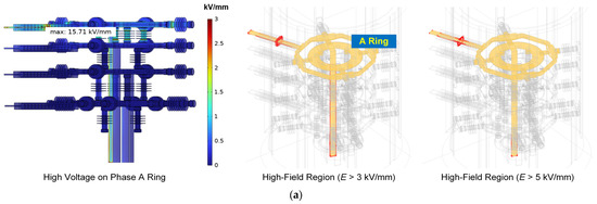
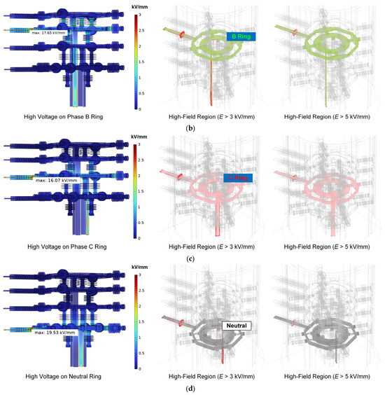
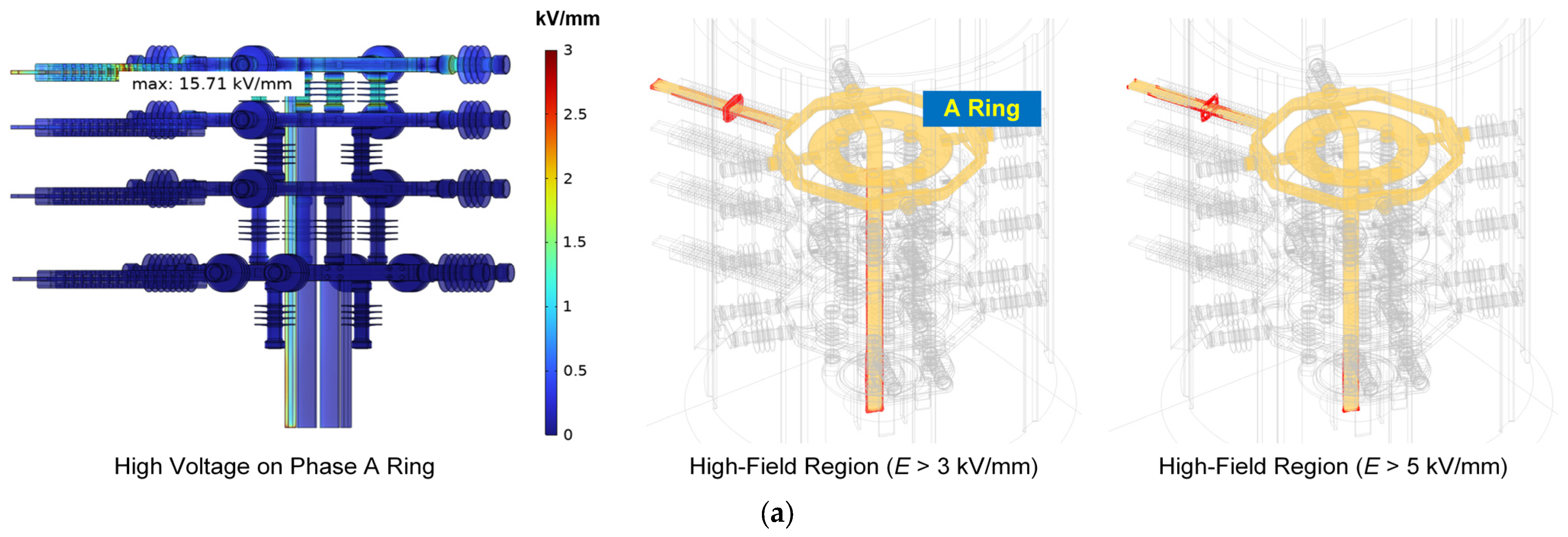
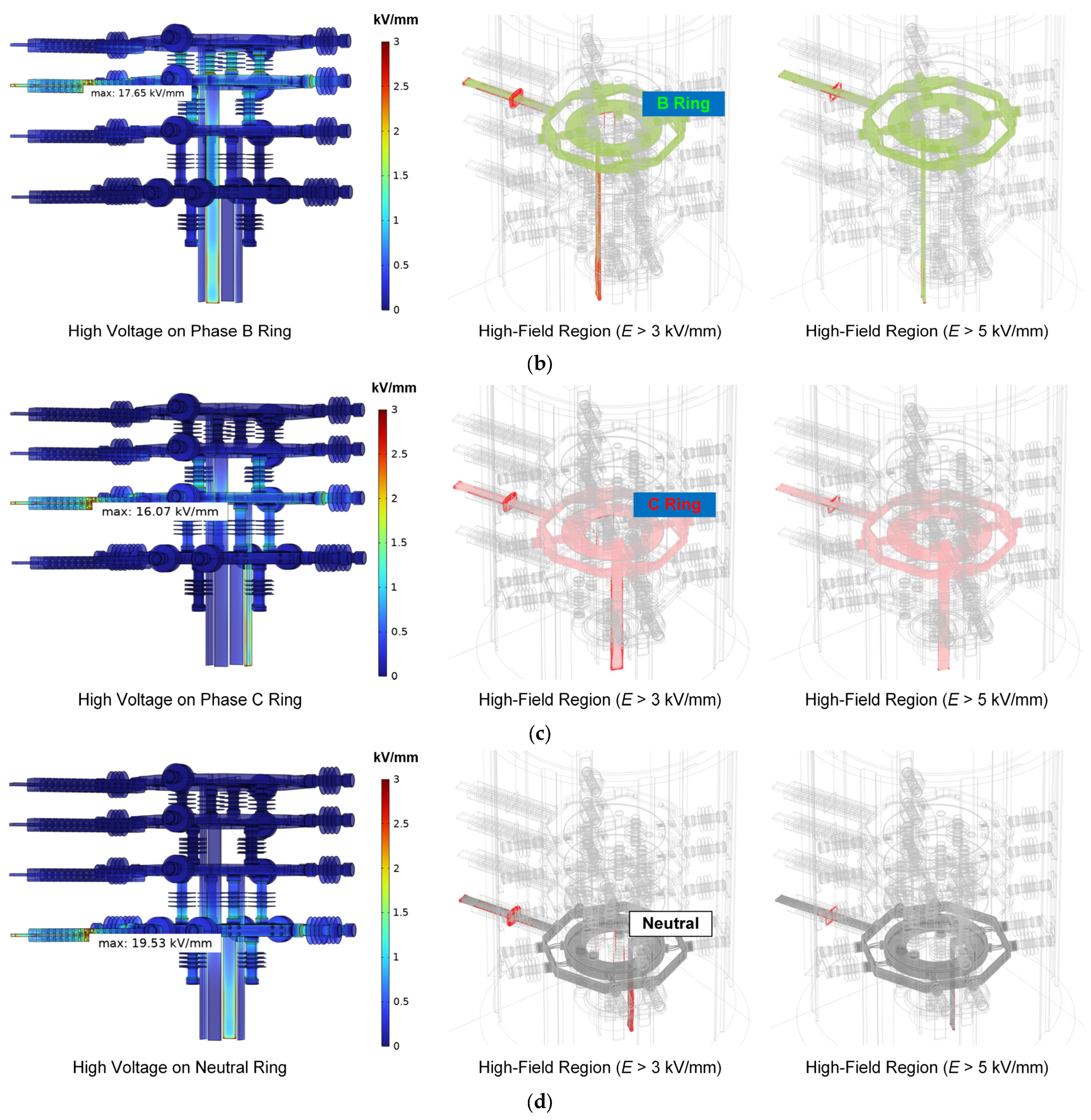
To further investigate the concentration of the electric field, the maximum field value and high-field region during the 95 kV test were analyzed, the results of which are shown in Figure 6. It can be seen that for all the configurations, the maximum electric field occurs at the central part of the inlet PTFE bushing. The maximum value reaches 15.71 kV/mm, 17.65 kV/mm, 16.07 kV/mm and 19.53 kV/mm for the high-voltage excitation on the A ring (Figure 6a), B ring (Figure 6b), C ring (Figure 6c) and neutral ring (Figure 6d), respectively. When this level of electric field is applied to the air or PTFE material, it is easy to generate partial discharge or even electric breakdown.
Figure 6.
The electric field distribution and high-field region (“red zone”) of the insulation system when a 95 kV r.m.s high voltage is applied to the (a) phase A ring, (b) phase B ring, (c) phase C ring and (d) neutral ring.
The high-field region (red zone) in Figure 6 also indicates the weakest point of the insulation system. When the high-field threshold is set to 3 kV/mm, the “red zone” includes (1) the gap between the PTFE bushing and outer walls, and (2) edges of the inlet and outlet busbars. If the threshold increases to 5 kV/mm, then the high-field region will shrink to the bushing–wall gaps. These results indicate that the wall–bushing gap will become the weakest point of electrical insulation during type tests and on-site operation, and the end part of the inlet and outlet busbars also requires optimization to further increase the insulation strength.
3.2. Simulation of Temperature Rise
3.2.1. Steady-State Temperature Rise
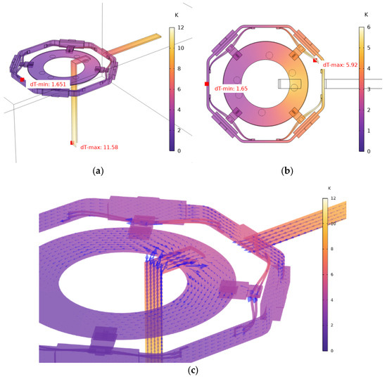
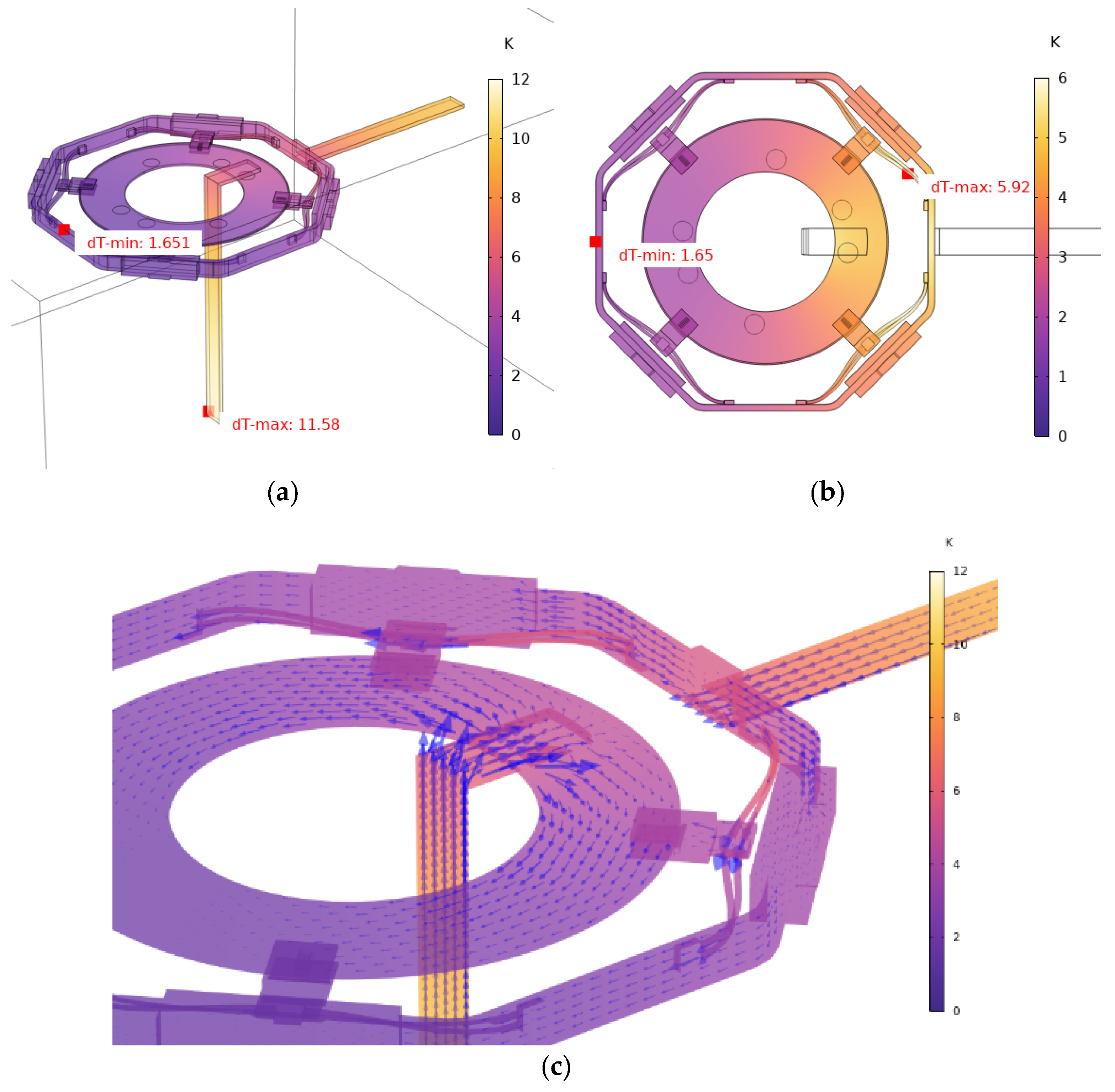
Figure 7 shows the temperature rise (ΔT = T − T0, with the ambient temperature T0 = 20 °C) distribution of the conductor system under the 640 A (r.m.s., 50 Hz) load. The simulation results reveal that the maximum temperature rise occurs at the bottom end of the outlet copper busbar, with a ΔT of 11.58 K (Figure 7a). In contrast, the central sliding-ring assembly, including the outer frame, sliding contacts, and inner ring, exhibits a lower temperature rise, with a maximum ΔT of 5.96 K located at the connection cables (Figure 7b). This difference is attributed to the more effective heat dissipation of the central ring structure due to its larger surface area-to-volume ratio and the conductive heat transfer from the busbars towards the ring, which acts as an additional heat sink, as indicated by the heat flux vectors shown in Figure 7c.
Figure 7.
Steady-state temperature rise in (a) the overall view of the simplified model, (b) the central sliding ring, and (c) the heat flow (blue arrow) inside the copper conductor.
3.2.2. Current Density and Skin Effect
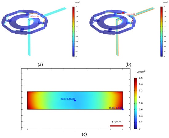
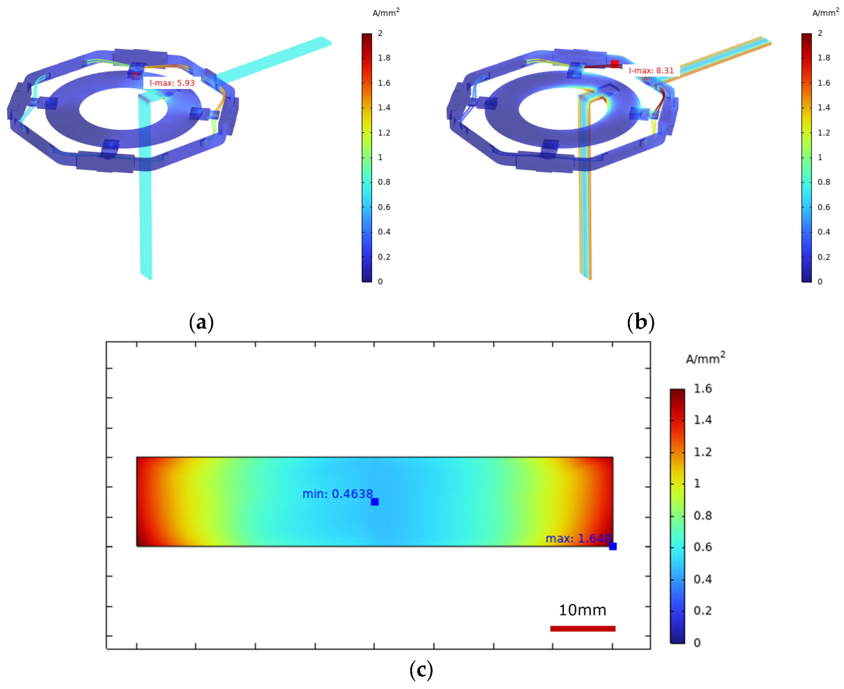
The skin effect is highly dependent on the operating frequency. As shown in Figure 8, the current density distribution changes significantly with frequency. At near-DC (0.01 Hz) in Figure 8a, the current density is uniform across the conductor cross-section, with a maximum of 5.93 A/mm2. At 50 Hz in Figure 8b, the skin effect becomes prominent, with the maximum current density increasing to 8.31 A/mm2 and shifting to the surface of stator–rotor connecting cables.
Figure 8.
Current density in the phase A ring at 640 A current under (a) near-DC (0.01 Hz) and (b) AC 50 Hz, and in (c) the inlet busbar cross-section at the input port.
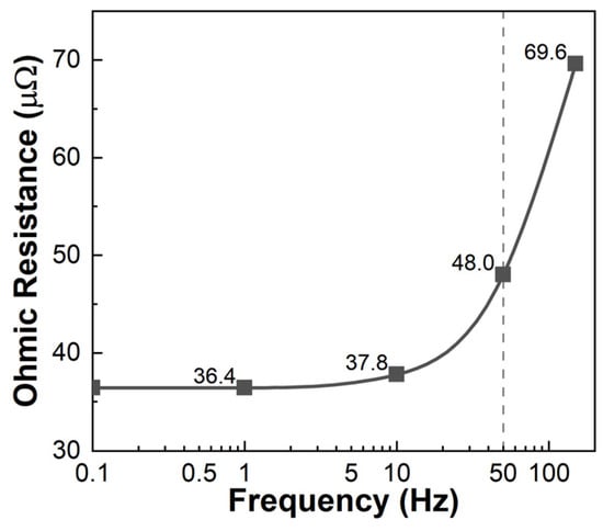
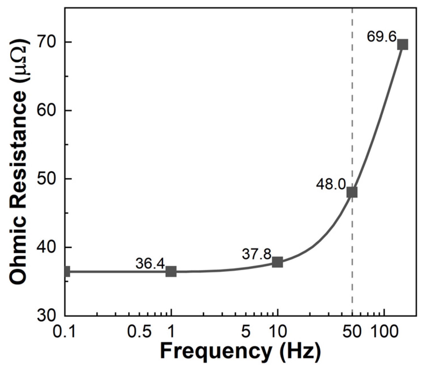
Figure 8c further indicates the pronounced skin effect when 50 Hz AC is applied to the system. The current density is highest near the outer surface of the busbar, reaching approximately 1.65 A/mm2, while it decays to about 0.46 A/mm2 in the core—only 27.8% of the surface value. The calculated skin depth for the copper busbar at 50 Hz is approximately 9.22 mm, which aligns well with the simulation results where the current density decays to about 30–40% of its maximum value within the first 10 mm from the surface. The above results indicate that the skin effect is strong in the current flow of AC 50 Hz frequency, which should not be neglected or replaced by a DC simulation. The non-uniform distribution leads to a 32% increase in conductor resistance when frequency rises from near-DC (0.1 Hz) to 50 Hz, as shown in Figure 9.
Figure 9.
The Ohmic resistance under various AC frequencies, from near-DC to 150 Hz.
To further validate the exclusion of the proximity effect, a comparative simulation of a full three-phase configuration was conducted. The results indicated that the maximum temperature rise discrepancy between the three-phase coupled model and the single-phase simplified model was within 1.4%. Therefore, the single-phase skin effect model provides sufficient precision for the thermal-performance evaluation of the 35 kV slip ring while maintaining computational efficiency.
3.2.3. Effects of Ambient Temperature, Heat Transfer Coefficient, and Current
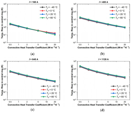
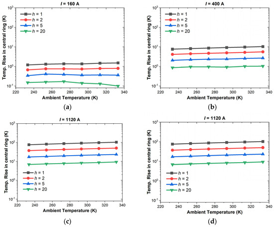
To study the effect of heat source (i.e., current load I), heat dissipation (convective heat transfer coefficient h) and outer environment (ambient temperature T0) on the temperature rise ΔT, parametric studies on the temperature rise were conducted and the temperature rise was recorded. It should be noted that h = 1∼5 W⋅m−2⋅K−1 represents typical natural convection in an enclosed or semi-enclosed chamber; h = 10∼20 W⋅m−2⋅K−1 corresponds to weak forced convection, which could be achieved if internal ventilation fans or cooling louvers are added to the outer shell. Moreover, since the main task of the simulation is to study the temperature rise in the sliding-ring system, only the maximum temperature rise at the central ring is recorded, as depicted in Figure 7b.
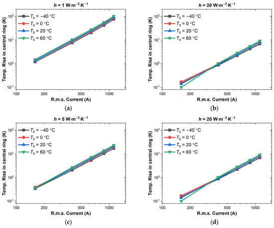
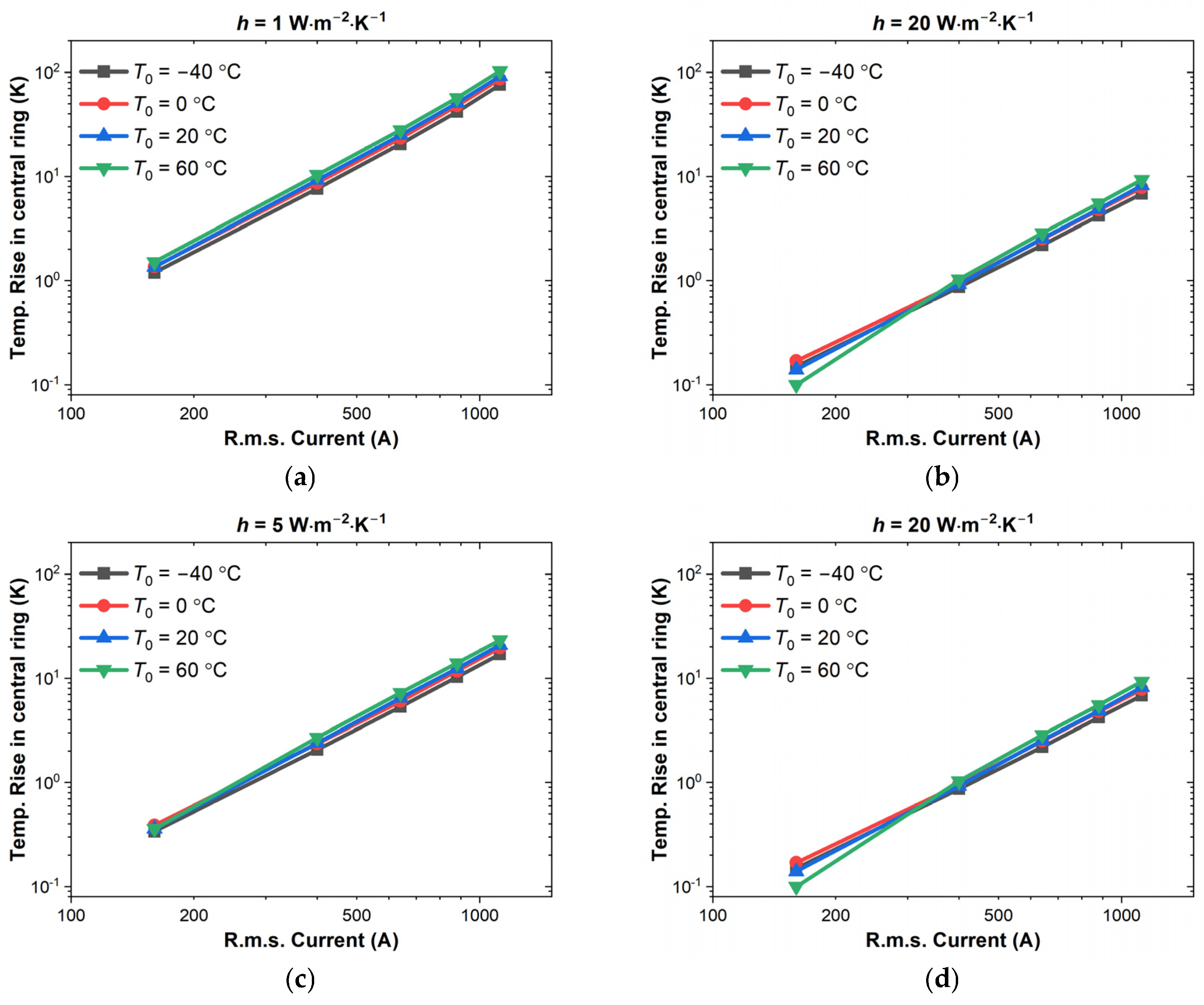
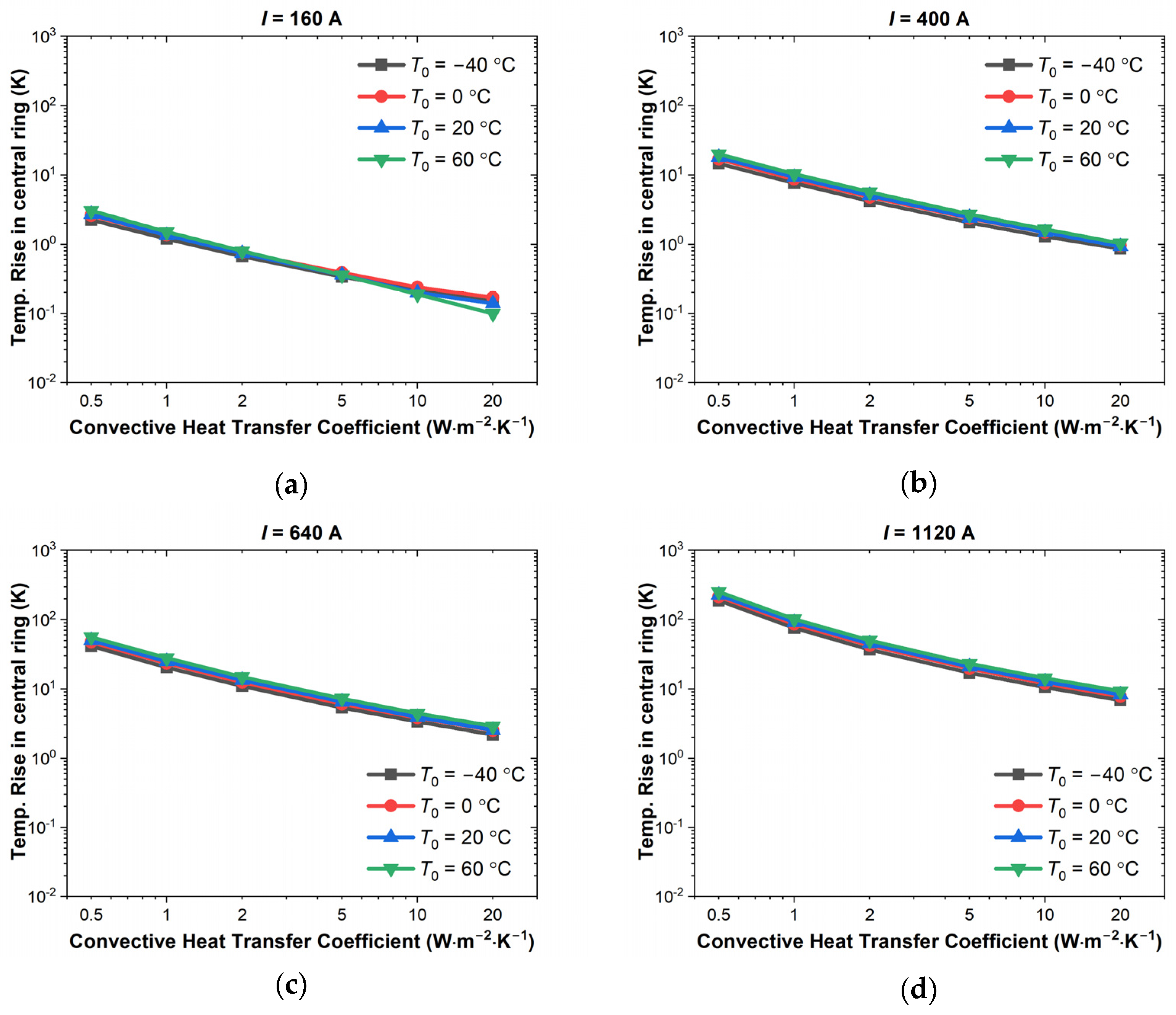
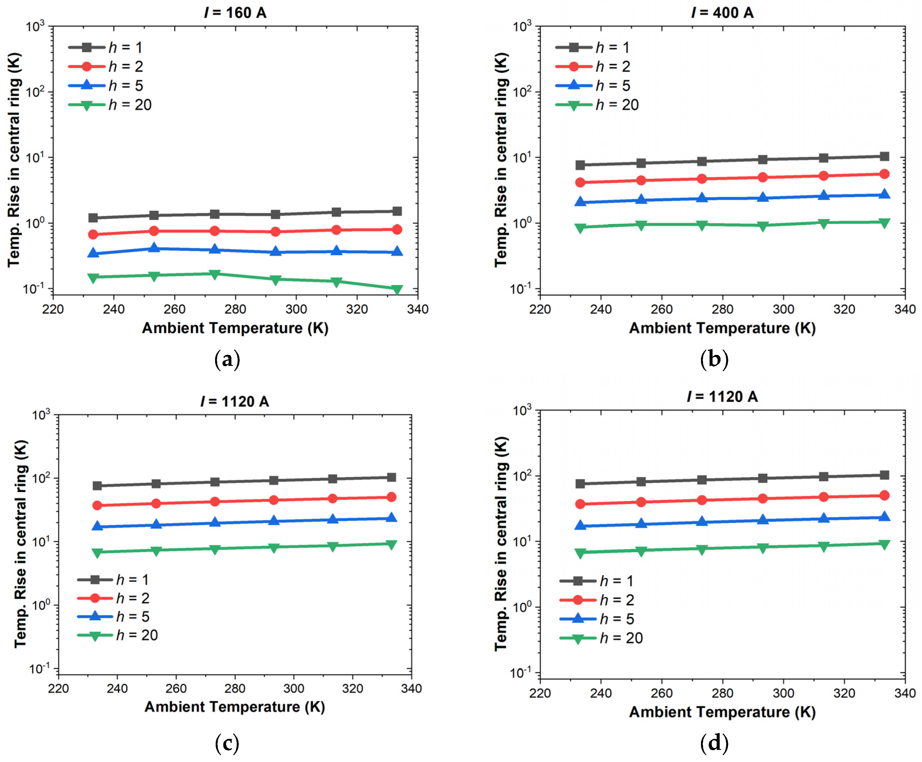
Figure 10 and Figure 11 depict the influence of current load I and convection heat transfer coefficient h on the temperature rise ΔT. The linear curves in the log-log plots indicate a power-law relationship between ΔT and I, as well as between ΔT and h. The difference is that the ΔT-I plots in Figure 10 indicate a positive power-law relationship, and the ΔT-h curves in Figure 11 indicate a negative correlation. These results are qualitatively reasonable since higher current leads to more generation of Joule heat, thus increasing the value of temperature rise. In contrast, higher dissipation through convective air flow can effectively cancel out the Joule heating and reduce ΔT. Figure 12 indicates the effect of ambient temperature on the temperature rise in log-log plots. Although weak, a positive linear correlation can be found, representing the increase in heat caused by the temperature-dependent copper resistance.
Figure 10.
Temperature rise in the central ring as a function of r.m.s. current load I when the convective heat transfer coefficient h is (a) h = 1 W·m−1·K−1, (b) h = 2 W·m−1·K−1, (c) h = 5 W·m−1·K−1, (d) h = 20 W·m−1·K−1.
Figure 11.
Temperature rise in the central ring as a function of convective heat transfer coefficient h when the r.m.s. current load I is (a) I = 160 A, (b) h = 400 A, (c) h = 640 A, (d) h = 1120 A.
Figure 12.
Temperature rise in the central contact ring as a function of ambient temperature T0 when the r.m.s. current load I is (a) I = 160 A, (b) h = 400 A, (c) h = 640 A, (d) h = 1120 A.
From the linear relationship shown in the log-log plot in Figure 10, Figure 11 and Figure 12, a multivariable log-log relationship can be used to evaluate the temperature rise:
where AI, Ah and AT0 are the coefficients related to load current I (in A), convective heat transfer coefficient h (in W) and ambient temperature T0; and C is a constant. Using the multivariable linear regression method, the temperature rise can be estimated by
The log-log expression in Equation (22) can be further converted to the power-law expression as
This model fits the simulation data with R2 = 0.99 and RMSE = 0.13, indicating effective prediction of the thermal performance of the slip ring under a wide range of operating conditions, greatly aiding in the design and rating of the prototype. The exponents in Equation (27) possess distinct physical meanings: the exponent 2.11 for current (h) aligns with Joule’s law (Q∝I2), where the additional 0.11 accounts for the non-linear increase in copper resistivity at higher temperatures. Similarly, the exponent −0.81 for the convection coefficient (h) reflects the inverse relationship in Newton’s law of cooling. This physical correspondence validates the model’s reliability for predicting thermal performance under varying operational conditions.
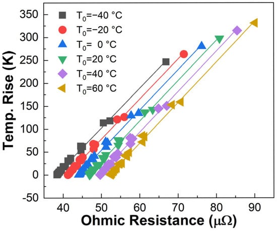
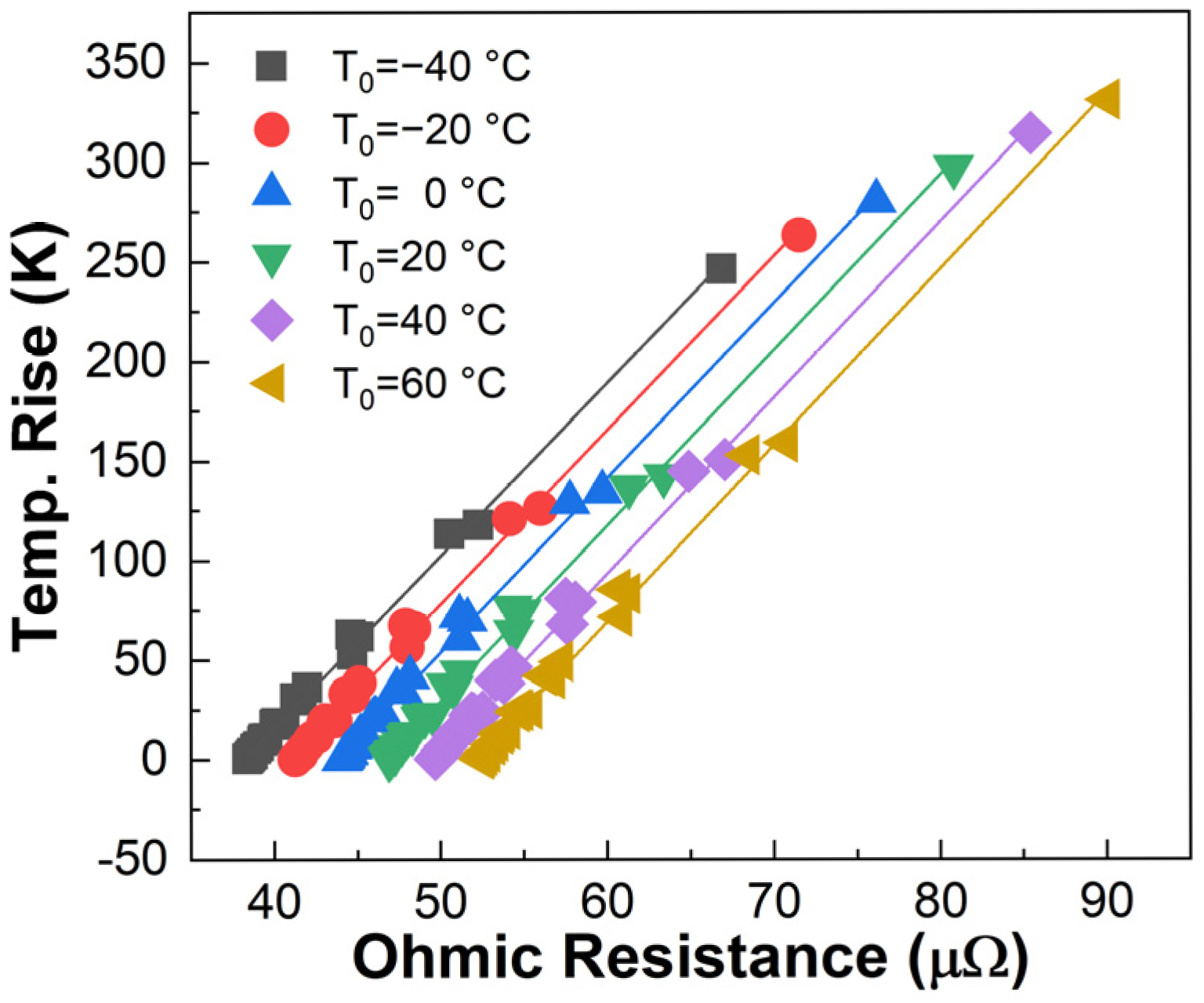
The Ohmic resistance serves as a critical bridge between electromagnetic excitation and thermal response. As illustrated in Figure 13, at a given ambient temperature, the temperature rise exhibits a robust linear correlation with the AC Ohmic resistance of the slip ring system. This linear dependency remains consistent across varying electrical and thermal boundary conditions, confirming that Joule heating is the predominant mechanism governing the system’s thermal behavior. Furthermore, these results suggest that online monitoring of the conductor’s resistance—derived solely from terminal electrical signals—could serve as a reliable indirect indicator for the real-time thermal state of the slip ring system in practical engineering applications.
Figure 13.
Correlation between temperature rise and Ohmic resistance of single-phase conductor in the slip ring under various thermal and electrical conditions (i.e., different I and h).
Another noticeable piece of information from the simulation is that the surface emissivity εrad is set to 0.05, representing polished copper. Sensitivity analysis based on the Stefan–Boltzmann law shows that increasing εrad to 0.5 or 0.8 (simulating oxidation or contamination) enhances radiative cooling and reduces the maximum temperature rise. Therefore, the assumption of 0.05 serves as a conservative ‘worst-case’ baseline, ensuring that the slip ring’s thermal-safety margin actually improves during long-term offshore operation as surface aging occurs.
4. Experimental Validation of the Simulation Results
4.1. Validation of the Electric Field Simulation
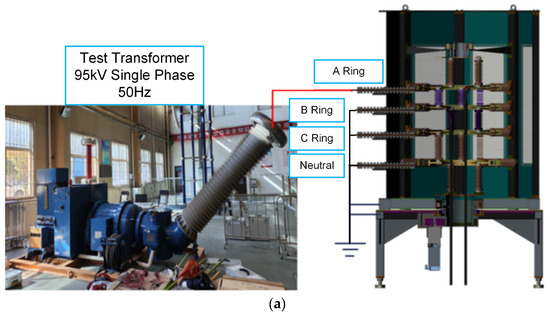
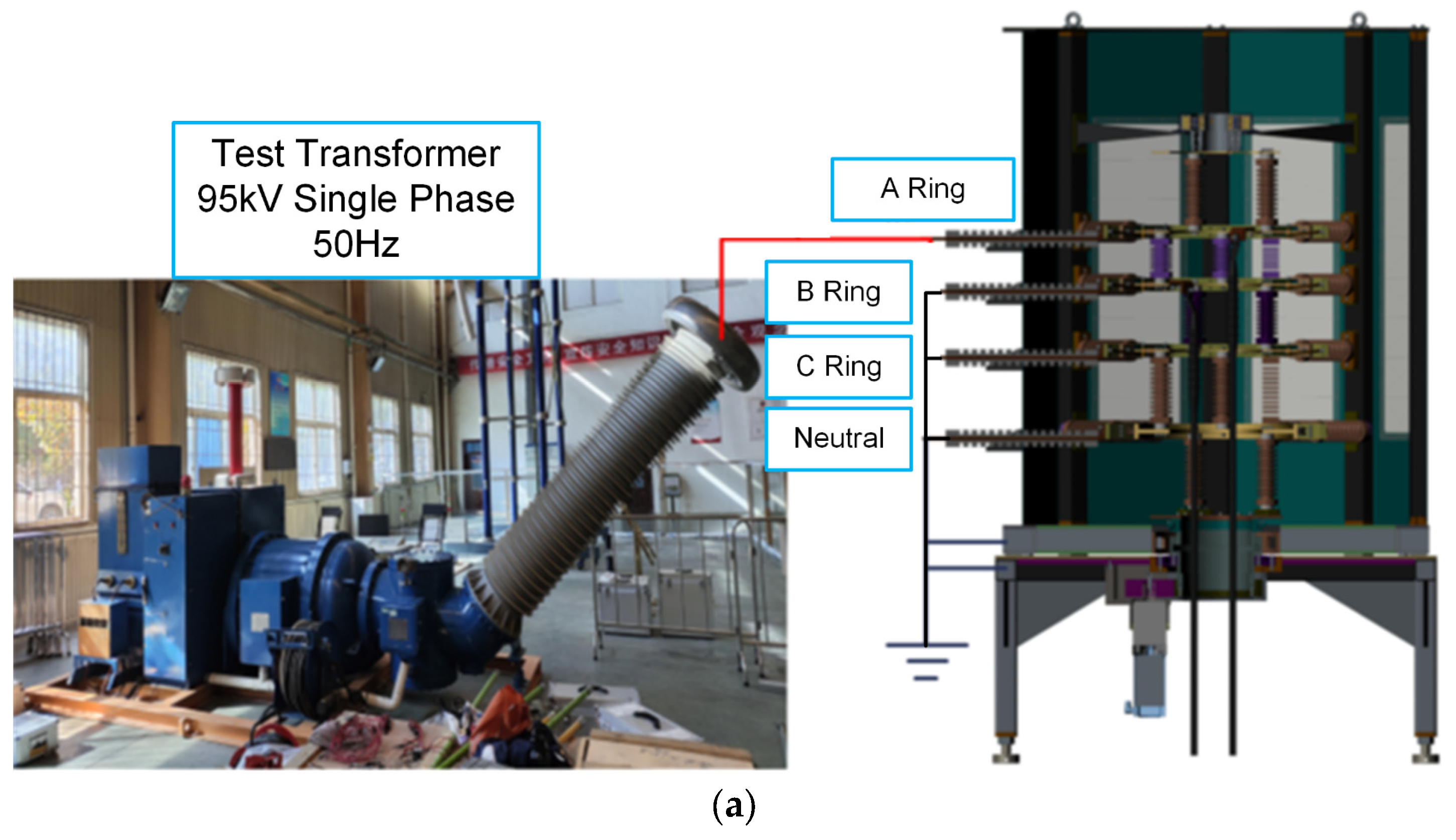
The AC breakdown test was conducted using the test platform shown in Figure 14a. This platform was built according to the IEC standard [10], in which a single-phase, 50 Hz test transformer was used to generate an AC test voltage and apply it to one of the test conductors (e.g., phase A ring in Figure 14a). Other conductors, including the copper rings and outer shell, are connected and grounded. During the AC breakdown test, the test voltage is continuously increased at a speed of 1 kV/s until breakdown occurs or the maximum value (i.e., 95 kV) is reached. The breakdown voltage or maximum voltage (if no breakdown occurs) is recorded as the test results.
Figure 14.
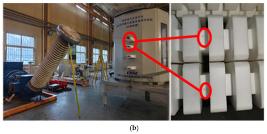
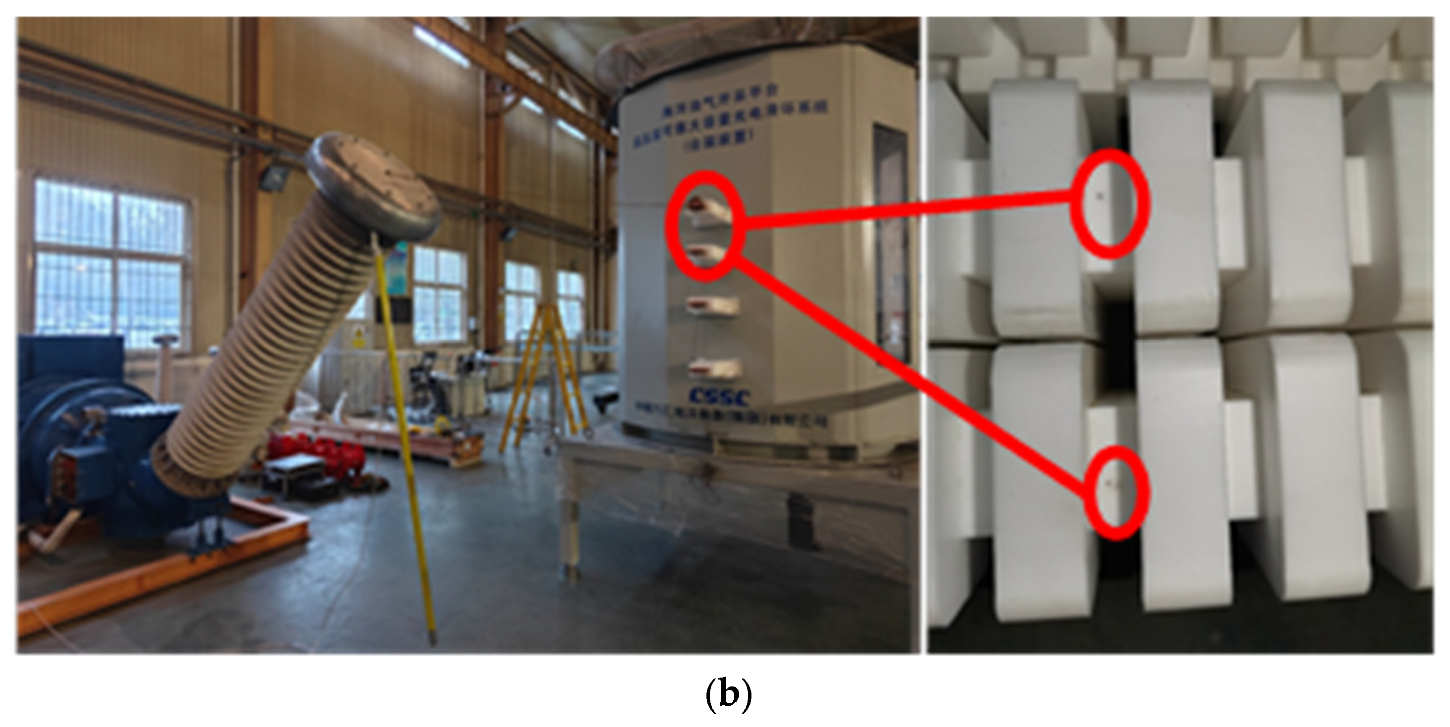
Experimental configuration for electric field simulation, including (a) AC withstand test setup for phase A ring and (b) breakdown failure observed at inlet PTFE bushing, all the testing platform was constructed by Shandong Taikai Testing Co., Ltd., Tai’an, China.
Table 4 indicates the results of the AC breakdown tests. It can be seen that all the breakdown occurs at the inlet PTFE bushing, which generates dark breakdown points shown in Figure 14b. Moreover, the AC breakdown voltage is nearly negatively correlated to the maximum electric field in the FEM simulation, which effectively confirms the correctness of the 3D electric field analysis.
Table 4.
Test results of AC breakdown experiments.
4.2. Validation of Temperature Rise Simulation
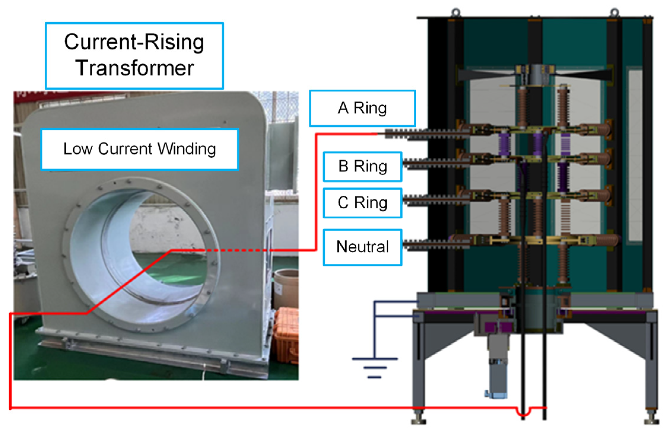
To confirm the thermal simulation, a high-current test was set up using a current booster to inject an AC ranging from 160 A to 1120 A (r.m.s.) into the slip ring prototype. The temperature rise at key points on the copper conductors was measured using 16 thermocouples after the system reached thermal equilibrium (i.e., the fluctuation of temperature rise is less than 2K in the time duration of 1 h). High-precision PT100 resistance temperature detectors (RTDs, ZC Sensors Technology Co., Ltd., Wuxi, China) with an accuracy of ± 0.15 K (level A) were utilized for temperature monitoring. Under each specific configuration, the temperature rise test was repeated three times, and the average value and standard deviation were recorded. The experimental configuration is shown in Figure 15.
Figure 15.
Experimental configuration for the temperature-raising test, all the testing platform was constructed by Shandong Taikai Testing Co., Ltd., Tai’an, China.
Table 5 compares the simulated and measured average temperature rises in the center rings (the maximum value) at different current levels, which demonstrates a good agreement between the FEM simulation and the experimental results. The error is within 15% across the entire current range, and it is below 8% at the rated current of 640 A, confirming the accuracy and reliability of the simplified magnetic–thermal coupling model and the adopted boundary conditions.
Table 5.
Comparison between simulated and experimental temperature rise.
4.3. Suggestions for Slip Ring Optimization
Based on the computational and experimental analyses, several targeted optimization strategies are proposed to enhance the insulation reliability and thermal management of the 35 kV electric-slip ring prototype:
- (1)
- Mitigation of electric field concentration: The 3D simulations and AC breakdown tests identified the inlet PTFE bushing and the gap between the bushing and the grounded shell as the critical insulation weak points, with maximum field strengths reaching 19.53 kV/mm. To address this, it is recommended to replace the current PTFE bushings with commercially available 35 kV epoxy bushings covered with silicone rubber sheds, which provide superior electric field grading and long-term stability in offshore environments. Additionally, applying proper chamfering or rounding to all internal copper-busbar edges is essential to eliminate localized field enhancement.
- (2)
- Thermal management and skin effect alleviation: Thermal simulations revealed that the 50 Hz AC leads to a 32% increase in AC resistance due to the skin effect, with current primarily crowding on the outer 9.22 mm of the busbars. To optimize performance, reducing the busbar thickness to below 10 mm or utilizing multi-core cables can mitigate the skin effect by reducing the unused core area while increasing the effective dissipation surface. Furthermore, the air convection coefficient (h) can be improved by installing ventilation louvers or fans on the enclosure. Finally, surface passivation or applying thin polymer coatings can significantly increase the infrared emissivity of the copper busbars from 0.05 to 0.5∼0.8, facilitating radiative cooling and effectively lowering peak temperatures.
5. Conclusions
This study conducts computational and experimental investigations on the insulation strength and temperature rise characteristics of a 35 kV electric-slip ring prototype for offshore Single-Point Mooring (SPM) systems. The following conclusions can be addressed:
- (1)
- The three-dimensional electric field simulation based on the finite element method (FEM) identifies the insulation weak points of the slip ring. Under the 95 kV r.m.s. power–frequency withstand voltage, the maximum electric field concentration occurs at the inlet PTFE bushing across all four excitation configurations (phases A, B, C, and neutral point), with the peak value reaching 19.53 kV/mm for the neutral ring. This value exceeds the breakdown strength of air (~3 kV/mm) and is close to that of PTFE (20–30 kV/mm), confirming the bushing–wall gap as the primary risk point for partial discharge or insulation breakdown.
- (2)
- The magnetic–thermal coupling simulation considering the skin effect captures the temperature rise behavior of the slip ring. At the rated 640 A r.m.s. current and 50 Hz frequency, the skin effect increases the copper-conductor resistance by 32%, leading to a non-uniform current density distribution (surface current density is 3.6 times that of the core). The maximum temperature rise at the central sliding ring is 5.96 K at 640 A current. Parametric analysis shows temperature rise has a positive power-law relationship with current load and ambient temperature, and a negative power-law relationship with the convective heat transfer coefficient. The established power-law prediction model (R2 = 0.99, RMSE = 0.13) estimates temperature rise under various operating conditions.
- (3)
- Experimental tests, including AC breakdown tests and high-current temperature rise tests, verify the simulation models. AC breakdown tests confirm all insulation failures occur at the inlet PTFE bushing, consistent with simulation results, and breakdown voltage correlates negatively with maximum simulated electric field. Temperature rise tests show simulated values agree with measured data, with errors within 15% across the 160–1120 A range, validating model simplifications and parameter selections.
Overall, this study establishes a technical framework integrating electric field simulation, thermal simulation, and experimental validation for high-voltage slip ring performance analysis. The findings clarify the insulation and thermal characteristics of 35 kV SPM slip rings, providing support for the design, operation, and fault prevention of similar offshore high-voltage electrical equipment.
In addition, it should be noted that the current EQS model assumes ωε is much greater than the electrical conductivity σ, representing the slip ring’s dielectric state during standard AC withstand tests. However, in offshore environments, factors like salt fog and aging can significantly enhance surface conductivity. This may shift the electric field from a permittivity-dominated to a conductivity-dominated distribution, potentially worsening field distortion. While providing a robust baseline for initial design, this study acknowledges the need for future research to incorporate dynamic degradation models for long-term reliability assessment.
Author Contributions
Conceptualization, H.W. and W.L.; methodology, Y.Z. and G.S.; validation, G.S., C.W. and J.Y.; writing—original draft preparation, F.L. and W.L.; writing—review and editing, H.W. and W.L.; visualization, W.L.; supervision, N.W. All authors have read and agreed to the published version of the manuscript, and are accountable for all aspects of the work in ensuring that questions related to the accuracy or integrity of any part of the work are appropriately investigated and resolved.
Funding
This work is financially supported by Major Science and Technology Projects of Jiangxi Province (20223AAE01002), China.
Data Availability Statement
The data is available upon request to the author.
Acknowledgments
The authors appreciate the assistance from Shandong Taikai Testing Co., Ltd., China in the experimental studies.
Conflicts of Interest
Authors Haiyan Wu, Nenghui Wang, Fangzhou Lu, Yunyi Zhu, Gaopeng Shuai, Chuanfeng Wang, and Jiayu Ye were employed by the CSSC Jiujiang Marine Equipment (Group) Co., Ltd. (Jiujiang 332005, Jiangxi, China). The remaining authors declare that the research was conducted in the absence of any commercial or financial rela-tionships that could be construed as a potential conflict of interest.
Nomenclature
The following symbols and abbreviations are used in this manuscript:
| Latin Symbols | |
| B | Magnetic flux density (T), vector |
| D | Electric flux density (C/m2), vector |
| d | Depth from the conductor surface (m) |
| E | Electric field strength (V/m), vector |
| f | AC frequency (Hz) |
| H | Magnetic field strength (A/m), vector |
| h | Convective heat transfer coefficient (W⋅m−2⋅K−1) |
| I | Root mean square (r.m.s.) current load (A) |
| J | Electric current density (A/m2), vector |
| k | Thermal conductivity (W⋅m−1⋅K−1) |
| n | Outward normal vector of the solid material surface |
| qc | Convective outward heat flux (W/m2) |
| qdis | Volumetric heat dissipation rate/Heat flux (W/m2) |
| qr | Radiative outward heat flux (W/m2) |
| qsrc | Volumetric heat generation rate (W/m3) |
| T | Temperature field (K) |
| T0/T∞ | Ambient temperature/Air temperature at infinite distance (K or °C) |
| Tref | Reference temperature for material properties (K) |
| Ts | Temperature at solid–fluid boundaries (K) |
| V/ | Electric potential/Phasor of the electric potential (V) |
| Greek Symbols | |
| α | Temperature coefficient of electrical resistance (K−1) |
| ΔT | Temperature rise (K) |
| δ | Skin depth of the conductor (m) |
| ϵ0 | Vacuum permittivity (F/m) |
| ϵr | Relative permittivity of insulation materials (Dimensionless) |
| ϵrad | Infrared emissivity of the material surface (Dimensionless) |
| μ | Magnetic permeability (H/m) |
| μ0 | Vacuum permeability (H/m) |
| μr | Relative permeability (Dimensionless) |
| ρ | Electric charge density (C/m3) |
| ρ0 | Electrical resistivity at the reference temperature (Ω⋅m) |
| σ | Electrical conductivity (S/m) |
| σrad | Stefan–Boltzmann constant (W⋅m−2⋅K−4) |
| ω | Angular frequency (rad/s) |
Abbreviations
| AC | Alternating Current |
| DC | Direct Current |
| EQS | Electro-Quasi-Static |
| FEM | Finite Element Method |
| FPSO | Floating Production Storage and Offloading |
| PD | Partial Discharge |
| PEC | Perfect Electric Conductor |
| PTFE | Polytetrafluoroethylene |
| r.m.s. | Root Mean Square |
| SPM | Single-Point Mooring |
References
- Hu, W.; Bao, J.; Hu, B. Trend and progress in global oil and gas exploration. Pet. Explor. Dev. 2013, 40, 439–443. [Google Scholar] [CrossRef] [Scilit]
- Küchler, A. High Voltage Engineering: Fundamentals—Technology—Applications, 5th ed.; Springer: Berlin, Germany, 2018; pp. 13–15. [Google Scholar]
- de Souza, M.F.; Queiroz, A.T.; Sotelo, G.G.; Monteiro, P.R.D.; Fortes, M.Z.; Polasek, A. Fault current limiters: A case study of protection and operational continuity for FPSOs. Electr. Eng. 2021, 103, 2035–2045. [Google Scholar] [CrossRef] [Scilit]
- Wang, B.; Hong, K.; Feng, C.; Zhang, H. The Investigation of Internal Turret Single Point Mooring Slip Ring Structure Design. In IOP Conference Series: Earth and Environmental Science; IOP Publishing: Bristol, UK, 2019; Volume 252, p. 022060. [Google Scholar]
- Feng, J.; Zou, T.K.; Sun, B. Analysis and Experiments on Current Distribution of 25MW High-Voltage Slip Ring. In Proceedings of the IEEE 6th Information Technology and Mechatronics Engineering Conference, Chongqing, China, 4–6 March 2022. [Google Scholar]
- Wu, H.; Zhang, Y.; Wu, H.; Shuai, G.; Li, W.; Mu, H. Numerical Simulation of Three-Dimensional Electric Field in a Prototype of 35 kV Offshore Single-Point Mooring Device. In Proceedings of the 2024 IEEE International Conference on High Voltage Engineering and Applications (ICHVE), Berlin, Germany, 18–22 August 2024. [Google Scholar]
- Haus, H.A.; Melcher, J.R. Electromagnetic Fields and Energy; Prentice-Hall: Englewood Cliffs, NJ, USA, 1989. [Google Scholar]
- IEC 60287-1-1:2006; Electric Cables—Calculation of the Current Rating—Part 1-1: Current Rating Equations (100% Load Factor) and Calculation of Losses—General. International Electrotechnical Commission: Geneva, Switzerland, 2006.
- Lienhard, J.H.V.; Lienhard, J.H., IV. A Heat Transfer Textbook, 6th ed.; Phlogiston Press: Cambridge, MA, USA, 2024. [Google Scholar]
- IEC 62271-1:2017; High-Voltage Switchgear and Controlgear—Part 1: Common Specifications for Alternating Current Switchgear and Controlgear. International Electrotechnical Commission: Geneva, Switzerland, 2017.
- Tabei, B.; Gole, A.M.; Kordi, B. Skin and Proximity Effect Calculation of a System of Rectangular Conductors Using the Proper Generalized Decomposition Technique. Energies 2024, 17, 2828. [Google Scholar] [CrossRef] [Scilit]

Disclaimer/Publisher’s Note: The statements, opinions and data contained in all publications are solely those of the individual author(s) and contributor(s) and not of MDPI and/or the editor(s). MDPI and/or the editor(s) disclaim responsibility for any injury to people or property resulting from any ideas, methods, instructions or products referred to in the content. |
© 2026 by the authors. Licensee MDPI, Basel, Switzerland. This article is an open access article distributed under the terms and conditions of the Creative Commons Attribution (CC BY) license.