Research on Localized Corrosion Monitoring of Cu Substrate Based on Discrete Fiber Optic Sensors

Abstract

The presence of corrosion on metal substrates can compromise the integrity of a structure. In this study, discrete fiber Bragg grating (FBG) sensing technology is used to monitor the corrosion process of a Cu surface in a corrosive environment. The surface morphology and nanostructures of corrosion products are observed to reveal their forms or structures. The results show that corrosion products are composed of loose or dense collections of micrometer/nanometer-sized particles in a crystalline state. Furthermore, this study experimentally explores how localized corrosion affects the sensing signal between an optical fiber and a corroded copper substrate. This phenomenon is also theoretically modeled using contact mechanics, enabling a semi-quantitative calculation of how corrosive particles influence Bragg wavelength. The wavelength shift trends of the four monitoring points over a period of 10 days were similar under the same corrosive environment. Results show that fiber Bragg grating sensors can identify the corrosion process in real time using wavelength demodulation methods. This study will lay the foundation for subsequent work on the precise monitoring of copper corrosion using fiber Bragg grating sensors.

1. Introduction

Copper-based materials have been widely used in buildings, Marine engineering and other fields due to their excellent physical and mechanical properties [1,2]. These metal materials usually function in highly challenging environments such as moisture, microorganisms, air, chemical pollution and large temperature differences. Throughout their service life, copper-based materials are affected by the external environment. Over time, copper-based materials are damaged due to corrosion. If not repaired or maintained in time, this will inevitably create considerable hidden dangers to the safe operation of facilities [3]. For instance, for copper-based material structures exposed to natural seawater, air, chemical solvents and other environments [4,5,6,7,8], long-term contact will cause external liquid molecules to interact with the passivation layer on the surface of the copper-based material, destroying the passivation layer and causing rust to form on the copper-based material. This leads to the formation of copper rust and corrosion cracking, further reducing the load-bearing capacity of structural components; ultimately, this leads to safety accidents [9,10,11]. It is reported that major safety accidents caused by the corrosion of metal-based structures occur worldwide every year [12]. Therefore, corrosion monitoring and accurate assessment of corrosion behavior are of great significance for providing early warnings of copper-based component damage, taking timely and effective maintenance measures, further ensuring the safe operation of infrastructure, and reducing maintenance and repair costs [13,14,15].

For the corrosion of metal-based components, traditional measurement techniques include polarized electrochemical impedance spectroscopy, acoustic emission, impact echo, ultrasonic waves, etc. [11,16]. Different monitoring methods exhibit limitations due to their distinct monitoring principles, such as low accuracy, high cost, surface damage, and secondary corrosion. To achieve accurate corrosion monitoring, especially early monitoring and continuous development, advanced non-destructive technologies, such as fiber optic sensing technology, have become a promising tool for structural health monitoring. Compared with traditional monitoring methods, optical fiber sensing technology features a small size, light weight, high sensitivity, high resolution, high precision, resistance to electromagnetic interference, and the required physical and chemical stability [17]. It can be interconnected to form a sensor network, enabling large-scale monitoring. At present, optical fiber sensing technology can be divided into discrete (point) optical fiber sensing technology and distributed optical fiber sensing technology. Fiber Bragg grating (FBG) sensors utilize the periodic refractive index changes within the fiber core to reflect specific light wavelengths, thereby achieving the measurement of strain, temperature, and other physical quantities. They have been widely applied to monitor the corrosion of reinforcing bars in concrete, steel plates, and steel bridges [18,19,20,21,22]. For example, Xu et al. [15] immersed coated steel substrates in a 3.5% NaCl solution, applying static loads to the steel every six days while recording the central wavelength changes in the grating sensor. This enabled real-time monitoring of the steel’s corrosion process, elucidating the interaction mechanism between loading and corrosion. Israel Sousa et al. [23] applied an FBG sensing system to detect the corrosion process of carbon steel plates in sodium chloride solutions. They compared this method with traditional ultrasonic and electrochemical detection techniques, demonstrating its effectiveness. Tan et al. [24] proposed a corrosion detection method for steel pipelines based on fiber optic sensors. By integrating this method with a scale analysis model, they achieved both corrosion visualization and early warning functions. Relative research has examined the reliability and applicability of the FBG sensing technique. However, studies on monitoring the corrosion of copper-based materials remain scarce, and there is a notable lack of investigation into the microstructure of the corrosion layer. Moreover, how corrosive particles affect the Bragg wavelength remains unclear. Therefore, employing FBG sensing technology is crucial for evaluating corrosion behavior in copper-based materials.

Therefore, in this paper, FBG sensing technology is used to study the corrosion dynamic behavior of copper-based materials under corrosive conditions. The experiment studies the corrosion process of copper-based materials and the microscopic morphology changes in the corrosion layer under corrosive conditions. Using the Hamaker model and contact mechanics theory, the adhesion force of corrosion particles to optical fibers and the shift in Bragg wavelength are semi-quantitatively calculated, which reveals the impact of corrosion behavior on optical sensing signals.

2. The Principle of FBG Sensing Technology

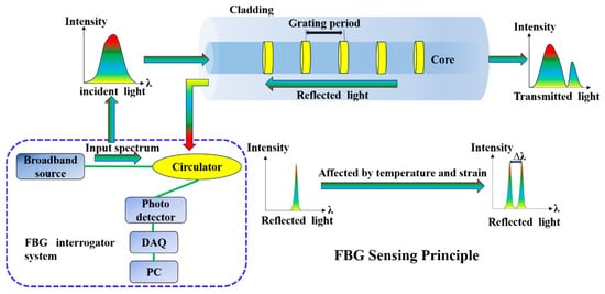
The FBG sensor is a type of sensor based on FBG technology. By exposing the single-mode fiber core to strong ultraviolet light, it induces the formation of periodic refractive index modulation of the grating structure. Figure 1 shows the inherent functional mechanism in FBG sensing [25]. The core principle is to measure changes in physical quantities by using the grating structure formed by the periodic refractive index changes in optical fibers. When the light from a broadband light source passes through the FBG, the light of a specific wavelength that meets the Bragg condition is reflected, while the light of other wavelengths continues to be transmitted.

Figure 1. Sensing principle of FBG.

Equation (1) shows the relationship between the Bragg wavelength ${\mathsf{\lambda }}_{\mathrm{B}}$ and the grating parameters [24]:

$${\lambda }_B=2n_{\mathrm{e}\mathrm{f}\mathrm{f}}\Lambda$$

(1)

Among them, ${\mathsf{\lambda }}_{\mathrm{B}}$ is the Bragg wavelength reflected by the Bragg grating, $n_{\mathrm{e}\mathrm{f}\mathrm{f}}$ is the effective refractive index, and $\Lambda$ is the grating period corresponding to the distance between two adjacent grating planes. When the grating is affected by temperature or strain, the interference caused by the interaction between light and the grating period leads to a shift in the Bragg wavelength ($\Delta {\lambda }_B$). This Bragg wavelength variation can be expressed as Equation (2) [26]:

$${\displaystyle \frac{\Delta {\lambda }_B}{{\lambda }_B}}=\left(1-P_e\right)\Delta \epsilon +\left({\xi }_f+{\alpha }_f\right)\Delta T$$

(2)

Among them, ${\lambda }_B$ and $\Delta {\lambda }_B$ are the initial Bragg wavelengths and their offsets, $\Delta \epsilon$ is the strain change, and $\Delta T$ is the temperature change. P_e, ${\xi }_f$ and ${\alpha }_f$ are respectively the photoelastic coefficient (theoretical value = 0.22), thermal optical coefficient and thermal expansion coefficient of the optical fiber. Since the reflection wavelength of the FBG is easily affected by the intersection point of strain and temperature, if the temperature remains constant or under the same operating conditions, when using the strain characteristics of the FBG for pressure measurement, the temperature cross-sensitivity effect [26] needs to be eliminated. That is, when $\Delta T=0$, the strain change can be simplified as Equation (3):

$${\displaystyle \frac{\Delta {\lambda }_B}{{\lambda }_B}}=\left(1-P_e\right)\Delta \epsilon$$

(3)

It can be found from Equation (3) that the change in strain is converted into the change in Bragg wavelength. When the metal surface where the Bragg grating sensor is located rusts, it can be used for real-time monitoring and recording. In addition, due to its rapid data acquisition capability, the Bragg grating sensor is optimized to track dynamic phenomena and rapid strain changes. These sensors are very effective for measuring discrete points along optical fibers, but multiple sensors may be required for distributed sensing. Therefore, in this research experiment, multiple Bragg grating sensors are arranged to achieve distributed monitoring of rust on the metal surface.

3. Materials and Methods

3.1. Design and Installation of FBG Sensor Specimens

In this experiment, purple copper plate (Cu1100, Jiangxi Jiangye Industrial Co., Ltd., Nanchang, China) is selected as the sample, in which the copper (Cu) content is ≥99.90%, and the total amount of other impurities is ≤0.10%. The size of the purple copper plate is 40 cm × 20 cm × 5 mm. The FBG sensor is composed of a single-mode fiber and five gratings. Among them, four red grating points are strain sensors, and one yellow grating point in the middle is a temperature compensation sensor.

Temperature compensation sensors are sensitive only to temperature, while strain sensors are sensitive to both temperature and strain. For temperature compensation sensors [26],

$$\Delta {\lambda }_{B0}=S_{T0}\mathsf{\Delta }T,$$

(4)

where $S_{T0}$ is the temperature sensitivity coefficient of the temperature compensation sensor. For strain sensors:

$$\Delta {\lambda }_B=S_{\epsilon }\mathsf{\Delta }\epsilon +S_T\mathsf{\Delta }T,$$

(5)

where $S_{\epsilon }$ and $S_T$ are the temperature and strain sensitivity coefficients of the strain sensor, respectively. Combining Equations (4) and (5) yields

$$\Delta {\lambda }_B=S_{\epsilon }\mathsf{\Delta }\epsilon +{\displaystyle \frac{S_T}{S_{T0}}}\Delta {\lambda }_{B0}$$

(6)

As shown in Equation (6), strain measurement errors caused by temperature are eliminated, achieving temperature compensation. Subtracting the temperature compensation term $S_T\Delta {\lambda }_{B0}/S_{T0}$ from the strain sensor reading $\Delta {\lambda }_B$ yields the wavelength shift caused by strain.

$$\Delta {\lambda }_{B\epsilon }=\Delta {\lambda }_B-{\displaystyle \frac{S_T}{S_{T0}}}\Delta {\lambda }_{B0}=S_{\epsilon }\mathsf{\Delta }\epsilon$$

(7)

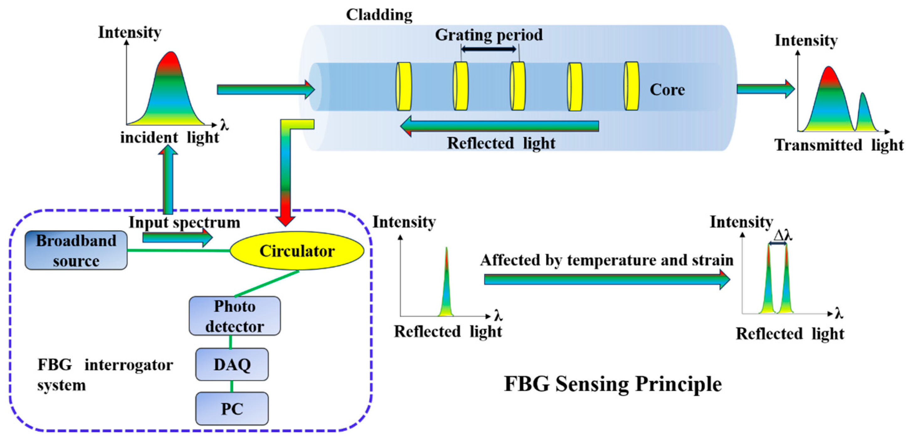
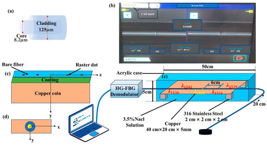
The bandwidth is 0.3 nm, and the side mode is greater than 15 dB. The single-mode fiber is made up of an acrylate coating and a fiber core, as shown in Figure 2a. In this study, acrylate-coated optical fibers are employed primarily due to the protective and mechanical properties of the acrylate polymer coating. The coating exhibits strong resistance to acidic, alkaline, and saline environments, allowing it to maintain structural integrity over extended periods in corrosive conditions. Furthermore, it adheres firmly to the fiber surface without peeling, even under bending or dynamic structural loads. More importantly, when coupled with the expansive stress generated by metallic corrosion products, the acrylate’s moderate elastic modulus enables efficient strain transfer from the corrosion-induced expansion to the FBG. This mechanism significantly enhances the sensitivity of corrosion monitoring. The main reason for using acrylate-coated optical fibers is that they have a good strain transfer rate with the substrate material and higher measurement accuracy. In the experiment, an optical fiber is used, and the optical fiber containing the grating is pasted parallel to the surface of the purple copper plate. Fiber gratings are fabricated by combining a 193 nm excimer laser with a phase mask, with a grating spacing of 6 cm. The optical fibers are bonded to the surface of the purple copper plate using ethyl cyanoacrylate resin, and the bonding length of the optical fibers is 40 cm. These parameters are adopted from prior studies [27]. To achieve a better bonding effect and enhance corrosion resistance, it is necessary to polish the surface of the purple copper plate with silicon carbide paper before bonding the optical fiber. For convenience of monitoring, a 2 m long pigtail fiber is reserved and directly spliced with a patch cord through optical fiber splicing technology and connected to the input port of the grating demodulation instrument. During the splicing process, it is particularly important to keep the optical fibers clean to minimize the loss caused by splicing to the greatest extent. The optical signal loss at the splicing point is 0.04 dB. The relevant parameters of the splicing machine are shown in Figure 2b. To present the situation of the optical fiber lying on the copper plate more clearly, its cross-section is configured, as shown in Figure 2c,d. The figures display a three-dimensional coordinate system. The origin of the x-y plane is located at the center point of the bare optical fiber, the X-axis is parallel to the contact surface between the copper plate and the coating, and the Y-axis is perpendicular to the X-axis. Furthermore, the direction of the fiber optic length arrangement serves as the Z-axis.

Figure 2. (a) fiber optic structure diagrams; (b) splicing machine-related parameters; (c,d) cross-sectional three-dimensional coordinate system; and (e) experimental setup diagram.

Make an acrylic experimental pool with dimensions of 50 cm × 20 cm × 5 cm. Place the purple copper plate with optical fibers lying horizontally on the surface of four small pieces of 316 stainless steel with dimensions of 5 × 5 × 5 mm. The central wavelengths λ₁₅₃₀, λ₁₅₃₆, λ₁₅₃₉ and λ₁₅₄₂ correspond respectively to the positions of 8 cm, 26 cm, 32 cm and 14 cm on the purple copper plate. At the beginning of the experiment, a 3.5% $\mathrm{N}\mathrm{a}\mathrm{C}\mathrm{l}$ solution was prepared, and then the copper plate was immersed in the $\mathrm{N}\mathrm{a}\mathrm{C}\mathrm{l}$ solution with a depth of 5 cm. The corrosion monitoring experiment lasts for 10 days. From the beginning of the experiment, a demodulator is used to monitor the grating points in real time. Five wavelengths of reflection spectra are obtained with central wavelengths of 1530 nm, 1533 nm, 1536 nm, 1539 nm and 1542 nm, respectively, and the strain and displacement at the four positions are monitored, as shown by the short red line in Figure 2e. The monitoring time interval is 100 ms. The surface morphology of the copper plate is observed under a 10× objective lens of an optical microscope. Then, it is taken out every two days, and the changes in its surface morphology are observed. After the experiment, the surface structure of the copper plate is observed, and the copper rust products on the surface are scraped for other related analyses. The experimental setup diagram is shown in Figure 2e.

3.2. Characterization and Test Methods

The surface and cross-sectional morphology of samples are analyzed using field emission scanning electron microscopy (FE-SEM, JEOL JMS-7500F, JEOL Ltd., Tokyo, Japan). A metallographic microscope (DMM-480AC, Shanghai Jinlai Optoelectronic Technology Co., Ltd., Shanghai, China) is used to observe the surface microscopic morphology. The structure and elemental composition of the aerugo are determined with a high-resolution transmission electron microscope (STEM, Talos F200X G2, Thermo Fisher Scientific, Wilmington, DE, USA) at 200 kV. The crystal structure is examined using a X-ray diffractometer (XRD, D8 Advance, Bruker Co., Karlsruhe, Germany) with Cu Ka radiation ($k=1.5418\AA$) in the 2θ range from 10 to 90° at 40 mA and 40 kV.

4. Results

4.1. Surface Morphology of Copper Corrosion

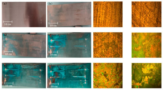
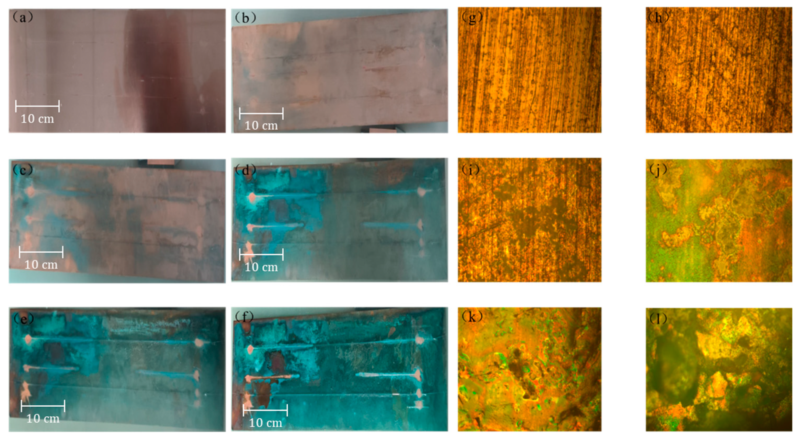
Figure 3a–f show the images of the original copper plate and the surface corrosion of the copper plate. It can be seen that the surface of the uncorroded purple copper plate is smooth, presenting a light brown metallic luster similar to that of copper plates. Under corrosion by NaCl solution, scattered dark areas appeared on the surface of the purple copper plate, and a small part of the end area showed a light green color. As time increased (on the 2nd, 4th, and 6th days), the color of the dark areas on the surface of the copper plate gradually deepened. In addition, the green areas gradually expanded, and the surface of the optical fiber turned green. On the 8th and 10th days, it can be clearly observed that the green color on the entire surface of the copper plate deepened, and large-scale blue-green product clusters appeared on the surface of the copper plate and the optical fiber, as shown in Figure 3d,f. To preliminarily observe the evolution of the microscopic morphology of the surface of the copper plate, Figure 3g–l show the corresponding microscopic morphologies of the copper plate under different immersion times in NaCl solution. Combining Figure 3a–l, it can be seen that at the beginning of the experiment, small green dots gradually appeared on the copper surface, as shown in Figure 3h; next, as the number of green dots increased, small green clusters gradually formed on the copper surface, as shown in Figure 3i. As time increased, large areas of blue-green products began to appear on the copper surface and some pitting occurred. This is because the NaCl solution could easily penetrate through the pores in the corrosion edge, resulting in the formation of obvious corrosion pitting, as shown in Figure 3j,k. As the experiment progressed, the corrosion products on the copper surface gradually increased and interconnected, forming large areas of copper rust products and generating obvious protrusions, as shown in Figure 3l.

Figure 3. (a–f) surface morphology images of copper plate on days 0, 2, 4, 6, 8 and 10. (g–l) microscopic morphology images of the copper plate on days 0, 2, 4, 6, 8 and 10.

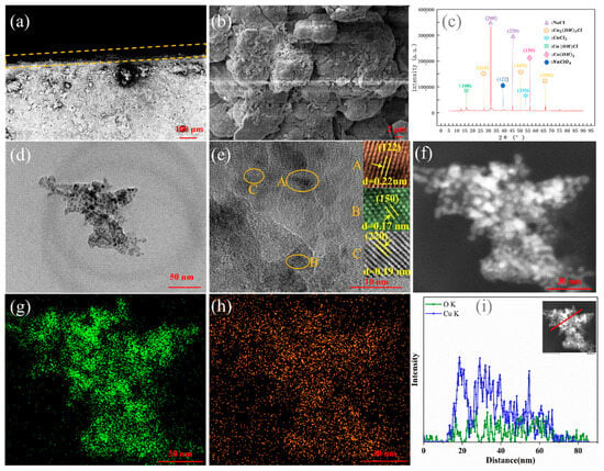
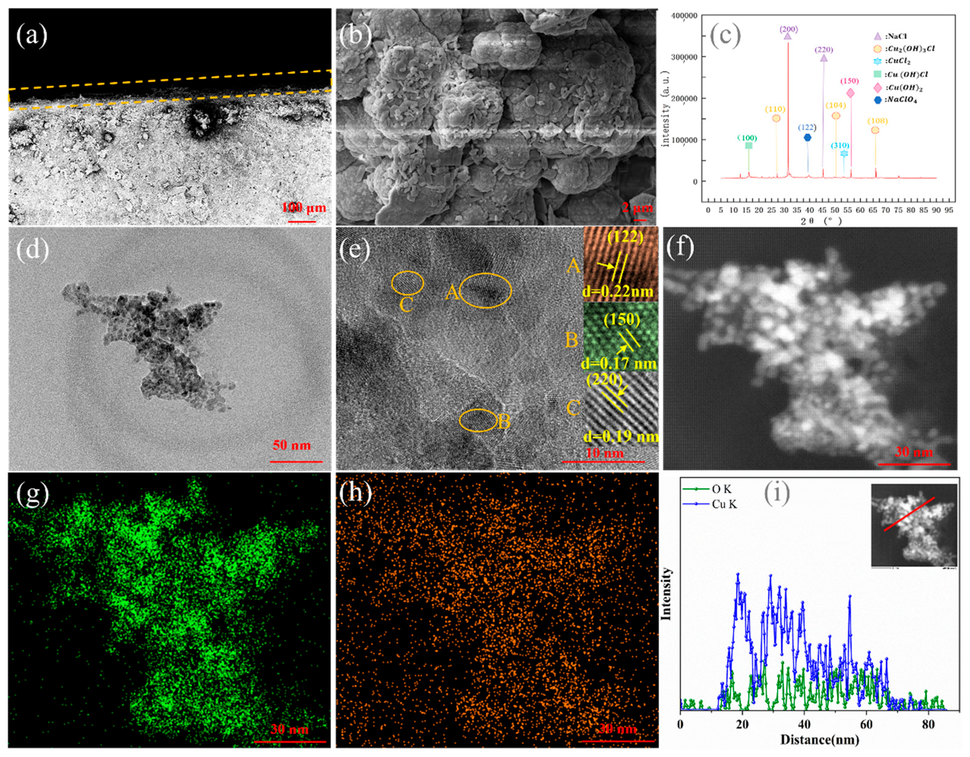
The cross-sectional SEM image of the sample of copper after 10 days of corrosion is shown in Figure 4a. It can be seen that a corrosion layer has formed on the surface of the copper substrate. Figure 4b shows the SEM image of the corrosion products on the surface of copper. The surface is uneven, and the corrosion products present as loose or dense collections of particles. The crystal structure of the corrosion products is further analyzed by XRD in Figure 4c. The corrosion products formed are mainly composed of Cu₂(OH)₃Cl, Cu(OH)Cl, CuCl₂, Cu(OH)₂, NaClO₄, and NaCl. The NaCl derives from corrosive liquid. The XRD peaks indicate that the primary three peaks, including (110), (104), and (108), can basically be assigned to the standard characteristic peaks of cube berzelianite (Cu₂(OH)₃Cl, JCPDS Card 30−0473). The main diffraction peaks (53.529°) of CuCl₂ corresponded to the (310) planes (JCPDS 34−0198). The peaks at 15.952° can be assigned to the (100) crystal planes of the Cu(OH)Cl (JCPDS 51−0400), respectively. The peaks at 53.210° and 39.654° are assigned to the (150) and (122) crystal planes of the Cu(OH)₂ and NaClO₄ (JCPDS 13−0420 and JCPDS 08−0494), respectively. According to the XRD pattern, it was confirmed that the corrosion products of copper were composed of a multi-component crystal structure [28].

Figure 4. (a) The cross-sectional and (b) surface SEM images of the corrosion products. (orange dashed line: The boundary of the corrosion layer) (c) XRD pattern of the corrosion products. (d) TEM and HRTEM images (e) of the corrosion products, and the inset is the filtered lattice fringes. (letters A, B, and C represent the lattice fringes at three different positions.) (f) A high-magnification TEM image. The EDX elemental (g,h) mapping and (i) line scan. The STEM image is shown in the inset.

To further analyze the nanostructure of the corrosion products, TEM analysis is indispensable. As shown in Figure 4d, the nanostructures of the corrosion products are composed of stacked nanoparticles. Figure 4e shows the HRTEM image in Figure 4d, presenting some clear irregular nanostructures. Meanwhile, local lattice fringes are observed in the HRTEM image, indicating that there is an order (atomic clusters) in the crystal within a short (or medium) distance range. It is seen from the fast Fourier transforms’ (FFT) patterns that the lattice with interplanar spacing of 0.22 nm, 0.17 nm and 0.19 nm corresponds to the (122), (150) and (220) planes, respectively. The result agrees with the result obtained by the XRD. In addition, the nanostructures are stacked on top of each other, and obvious nanoscale interface contacts at the stacking boundaries can be observed. Figure 4f is a high-magnification TEM image of the corrosion products. It can be seen from the EDX elemental mapping (Figure 4g,h) that the corrosion layer includes O and Cu elements [29,30]. EDX-ray line scanning (Figure 4i) revealed that the strength of the Cu element is higher than that of the O element, which might be related to the composition of other elements. The scanning TEM (STEM) image is shown in the inset.

In order to clearly understand the formation process of the corrosion layer, it is necessary to analyze the reaction process. The corrosion process of copper involves various chemical reactions, which depend on the environmental conditions. The relevant chemical reaction mechanisms are as follows [31,32]:

(1) Oxidation reaction: Copper is first oxidized to copper ions (Cu²⁺) in solution and then combines with chloride ions (Cl⁻) to form copper chloride ($\mathrm{C}\mathrm{u}\mathrm{C}{\mathrm{l}}_2$), which is a yellowish-green crystal.

$${\mathrm{C}\mathrm{u}}^{2+}+2\mathrm{C}{\mathrm{l}}^{-}\to \mathrm{C}\mathrm{u}\mathrm{C}{\mathrm{l}}_2$$

(8)

(2) The formation of rust: In a chlorine-containing environment, harmful rust forms on the surface of copper, such as copper hydroxide (Cu(OH)₂, blue precipitate) and basic copper chloride (Cu₂(OH)₃Cl, Cu(OH)Cl, green or bluish-green precipitates).

$${\mathrm{C}\mathrm{u}}^{2+}+2\mathrm{O}{\mathrm{H}}^{-}\to \mathrm{C}\mathrm{u}{\left(\mathrm{O}\mathrm{H}\right)}_2$$

(9)

$${\mathrm{C}\mathrm{u}}^{2+}+\mathrm{C}{\mathrm{l}}^{-}+\mathrm{O}{\mathrm{H}}^{-}\to \mathrm{C}\mathrm{u}\left(\mathrm{O}\mathrm{H}\right)\mathrm{C}\mathrm{l}$$

(10)

$$2\mathrm{C}\mathrm{u}\left(\mathrm{O}\mathrm{H}\right)\mathrm{C}\mathrm{l}+\mathrm{O}{\mathrm{H}}^{-}\to \mathrm{C}{\mathrm{u}}_2{\left(\mathrm{O}\mathrm{H}\right)}_3\mathrm{C}\mathrm{l}+\mathrm{C}{\mathrm{l}}^{-}$$

(11)

The corrosion products formed have a loose structure and cannot effectively protect the copper substrate. Instead, they will aggravate the corrosion.

4.2. Sensing and Dynamic Monitoring of Copper Corrosion

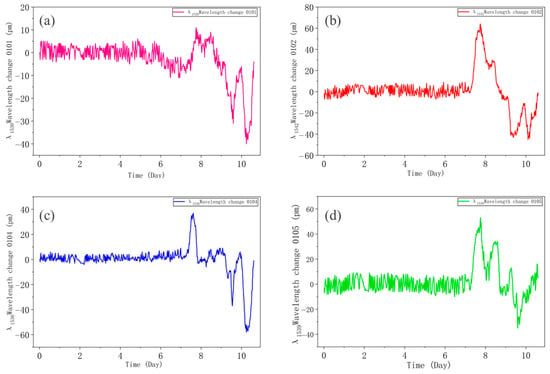
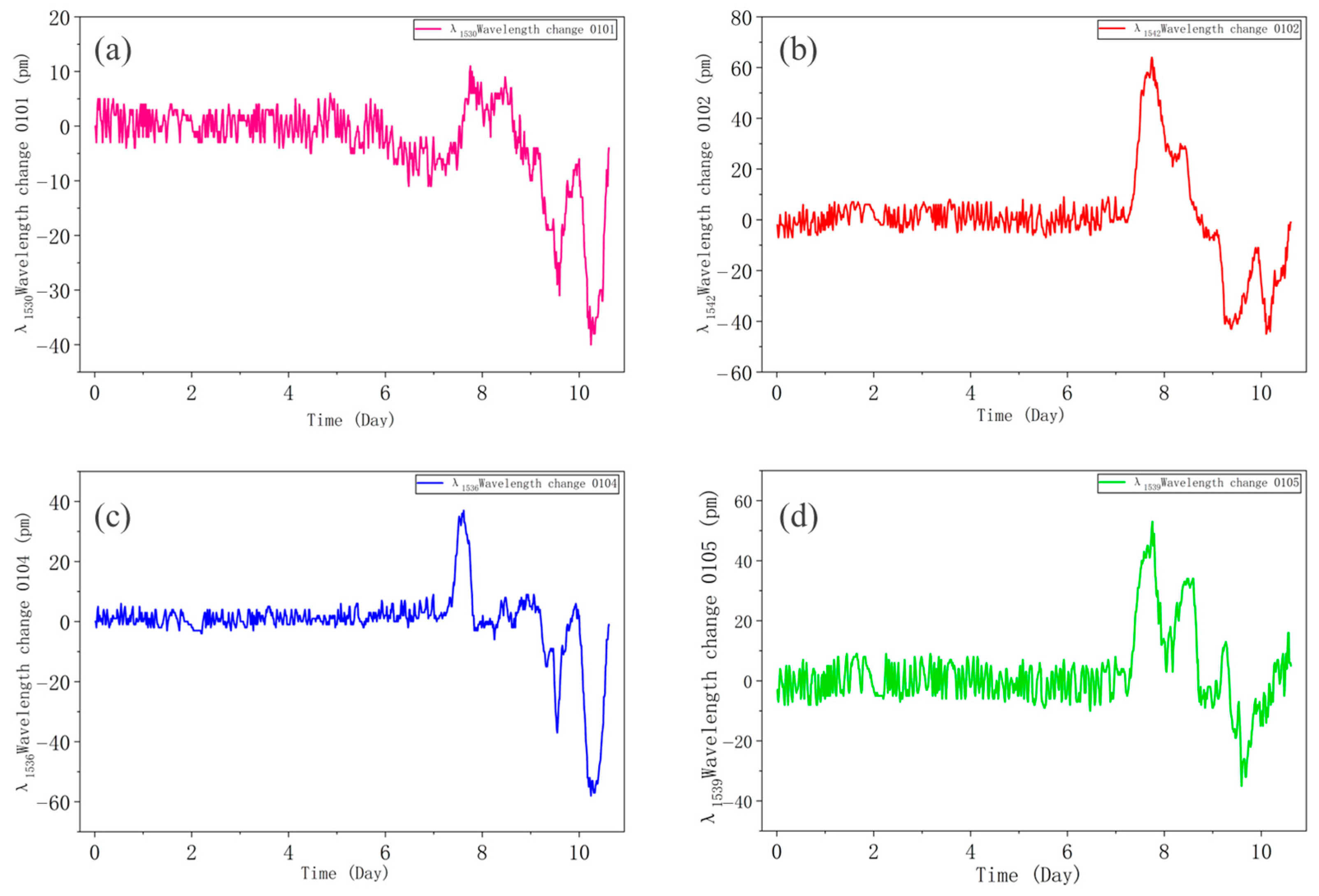
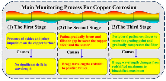
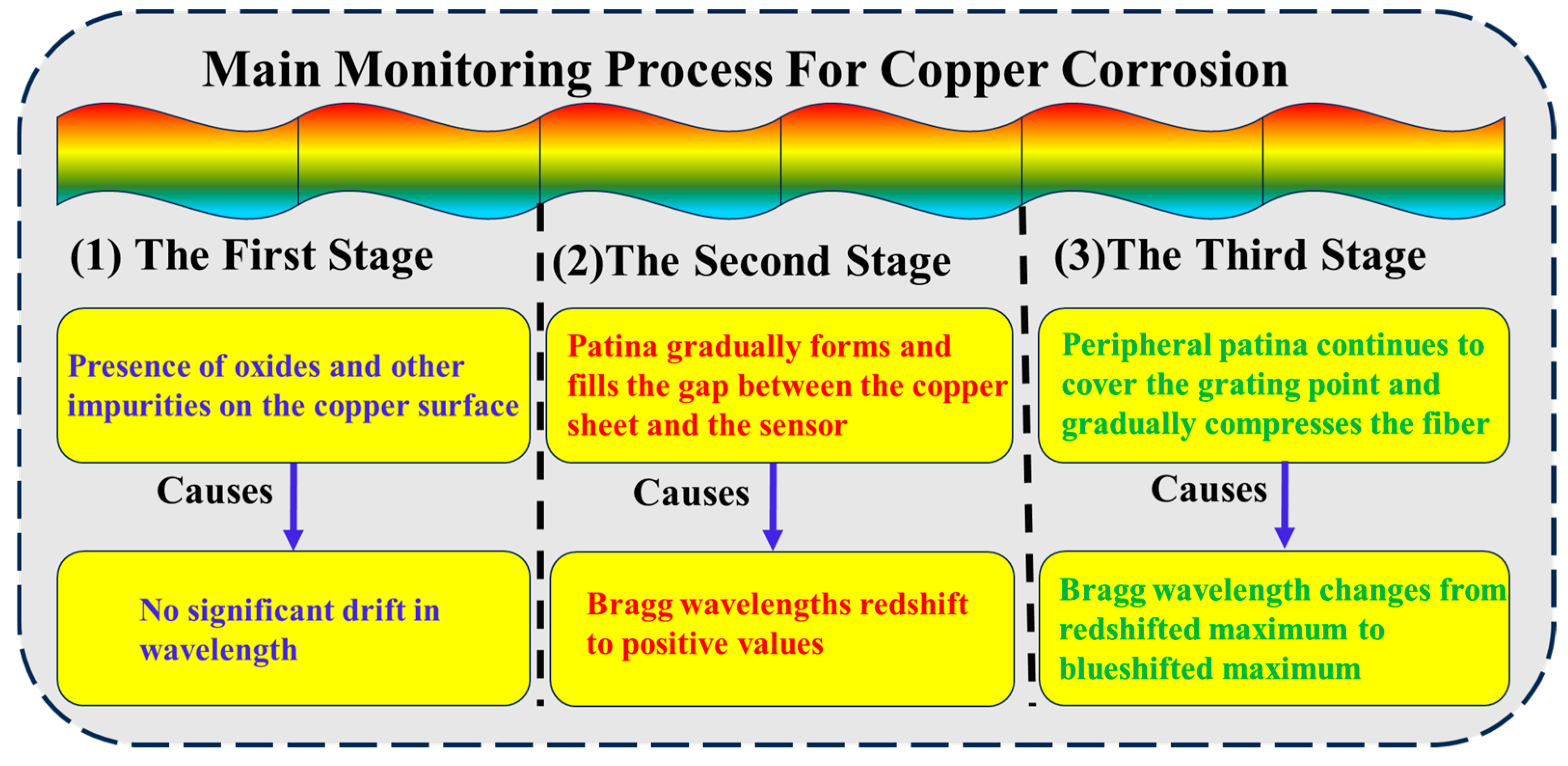
As shown in Figure 5, it depicts the variation in the Bragg wavelength of different strain sensors at different positions on the copper plate over time after temperature compensation [33]. In Figure 5a, the pink curve represents the variation curve of the wavelength of the 0101 sensor (λ₁₅₃₀) over time. In Figure 5b, the red curve represents the variation curve of the wavelength of the 0102 sensor (λ₁₅₄₂) over time. In Figure 5c, the blue curve represents the variation curve of the wavelength of the 0104 sensor (λ₁₅₃₆) over time. The green curve in Figure 5d represents the variation curve of the wavelength of the 0105 sensor (λ₁₅₃₉) over time. The negative Bragg wavelength drift that occurs in the four figures is due to the fact that the strain sensor is initially tightened and adhered during installation. As the corrosion time increases continuously, the optical fiber deforms, causing the tension on the strain sensor to decrease and gradually turn into a compressive force, thereby resulting in a blue shift in the wavelength and a negative value. In the four pictures in Figure 5, the corrosion is roughly divided into three stages. The first stage is characterized by the initial stage of corrosion. Due to the possible presence of a small number of oxides and other impurities on the copper surface, the corrosion of the copper sheet occurs relatively slowly over a long period of time. During this phase, there is no significant drift in the Bragg wavelength, as shown in the relatively gentle curve at the front of Figure 5. The second stage encompasses the early and middle stages of corrosion. The Bragg wavelength change is above the coordinate axis and reaches the highest point. This is because copper rust gradually forms and fills the gap between the copper sheet and the sensor, causing the strain sensor at the grating point to be stretched. This causes a red shift in the Bragg wavelength, which shows a positive value and redshifts to the maximum value. Then the third stage encompasses the middle and late stages of corrosion. The Bragg wavelength shift changes from the maximum positive value to the maximum negative value. This is because the surrounding copper rust continuously covers and compresses the optical fiber, causing a blue shift in the Bragg wavelength. The three stages precisely correspond one-to-one with the observations of the surface morphology and microscopic morphology on days 0, 2, 4, 6, 8, and 10 in Figure 3. The results show that the FBG sensing system can not only detect the occurrence of corrosion events but also precisely locate the locations where they occur and quantify their severity, providing unprecedented spatial dimension information for assessing the structural health status. Figure 6 presents the main monitoring process diagram of copper corrosion. The combination of Figure 5 and Figure 6 can make it more convenient to analyze the entire process of the copper corrosion experiment. This provides certain references for real-time monitoring of the corrosion process of copper-based materials using FBG sensing technology and exploring the influence of corrosion behavior on optical sensing signals and its influence mechanism.

Figure 5. The drift in the Bragg wavelength over time. The variation curve of the wavelength of the 0101 sensor (λ₁₅₃₀) (a), the 0102 sensor (λ₁₅₄₂) (b), the 0104 sensor (λ₁₅₃₆) (c) and the 0105 sensor (λ₁₅₃₉) (d) over time.

Figure 6. Main monitoring flowchart of copper corrosion.

4.3. A Theoretical Model of the Relationship Between Surface Corrosion and Strain

When using discrete FBG sensing technology to monitor the changes in copper corrosion, the changes in strain are significantly converted into changes in wavelength ($\Delta {\lambda }_B$), enabling the fiber sensing technology to detect the strain caused by copper corrosion. In this study, the corrosion products remain on the copper substrate until the end of the experiment.

The primary corrosion product of copper in sodium chloride solution is Cu₂(OH)₃Cl. This precipitate adheres to optical fibers, exerting an adhesive force that is generally attributed to van der Waals forces. Considering the basic copper chloride precipitate as composed of numerous spherical particles, we first analyze the adhesion force exerted by a single Cu₂(OH)₃Cl particle on the optical fiber.

Hamaker [34] proposed a model suggesting that the van der Waals force $F$ between a particle and its attached substrate satisfies

$$F={\displaystyle \frac{AR}{6z_0^2}}$$

(12)

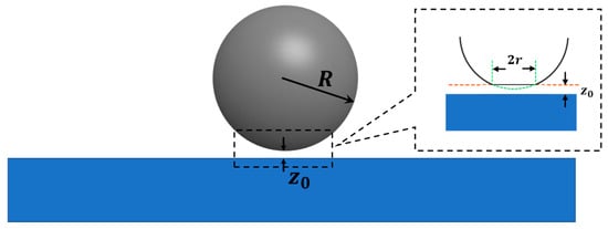
where $R$ is the particle radius, $z_0$ is the equilibrium distance between the particle and substrate ($z_0\approx 0.2\mathrm{n}\mathrm{m}$), and $A$ is the Hamaker constant, which depends on the dielectric properties of the particle, substrate, and surrounding medium, as shown in Figure 7.

Figure 7. Particle with radius $R$ adhering to the substrate. (The deformation of the particles and the substrate near the contact point is shown within the dashed box.)

The Hamaker constant $A$ can be calculated by using the Lifshitz theory [35]

$$A={\displaystyle \frac{3}{4}}{k}_{\mathrm{B}}T\left({\displaystyle \frac{{\epsilon }_1-{\epsilon }_3}{{\epsilon }_1+{\epsilon }_3}}\right)\left({\displaystyle \frac{{\epsilon }_2-{\epsilon }_3}{{\epsilon }_2+{\epsilon }_3}}\right)+{\displaystyle \frac{3h{\nu }_e}{8\sqrt{2}}}{\displaystyle \frac{\left(n_1^2-n_3^2\right)\left(n_2^2-n_3^2\right)}{\sqrt{n_1^2+n_3^2}\sqrt{n_2^2+n_3^2}\left(\sqrt{n_1^2+n_3^2}+\sqrt{n_2^2+n_3^2}\right)}}$$

(13)

where $k_{\mathrm{B}}$ is the Boltzmann constant, $T$ is the temperature, $\epsilon$ is the relative permittivity, $h$ is Planck’s constant, ${\nu }_e$ is the ionization frequency of the material (typically ${\nu }_e\approx 3\times {10}^{15}\mathrm{H}\mathrm{z}$), and $n$ is the refractive index. The subscripts 1, 2, and 3 denote the particle, substrate, and medium, respectively.

The Lifshitz theory disregards atomic structure, treating massive objects as continuous media, and derives the interaction forces between objects based on volumetric properties such as dielectric constant and refractive index.

In this study, 1 represents Cu₂(OH)₃Cl particles, 2 represents the optical fiber SiO₂, and 3 represents the NaCl solution. The values of the above physical quantities are $k_B=1.38\times {10}^{-23}\mathrm{J}/\mathrm{K}$, $T=300\mathrm{K}$, ${\epsilon }_1\approx 5,{\epsilon }_2\approx 3.5,{\epsilon }_3\approx 70,h=6.626\times {10}^{-34}\mathrm{J}·\mathrm{s},{\nu }_e\approx 3\times {10}^{15}\mathrm{H}\mathrm{z},n_1\approx 1.5,n_2\approx 1.45,n_3\approx 1.33$. From these values, the Hamaker constant $A=7.51\times {10}^{-21}\mathrm{J}$ for Cu₂(OH)₃Cl particles in NaCl solution with fiber SiO₂ can be obtained. For particles with a radius $R=1\mathsf{\mu }\mathrm{m}$, the adhesive force is

$$F={\displaystyle \frac{7.51\times {10}^{-21}\times {10}^{-6}}{6\times {\left(0.2\times {10}^{-9}\right)}^2}}\mathrm{N}=7.82\times {10}^{-8}\mathrm{N}$$

(14)

Due to slight deformations in the particle near the contact point, a contact area with radius $r$ is formed, as indicated by the dashed box in Figure 7. This radius $r$ is termed the contact radius, typically $r\approx 0.05R$. Nearly all the interaction forces between the particles and the substrate are concentrated within this contact area, resulting in a pressure of

$$p={\displaystyle \frac{F}{\pi r^2}}$$

(15)

If Cu₂(OH)₃Cl forms an adherent layer of thickness $D$ on the fiber surface, it can be regarded as composed of particles with a radius $R=D/2$ stacked together, as shown in Figure 8. For an adhered layer with a thickness $D=2\mathsf{\mu }\mathrm{m}$, the adhesive pressure $p=3.98\times {10}^6\mathrm{P}\mathrm{a}$.

Figure 8. An adherent layer of thickness D can be equivalently modeled as a stack of particles with radius $R=D/2$.

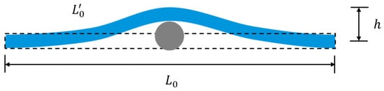
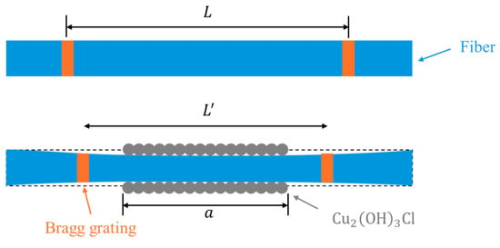
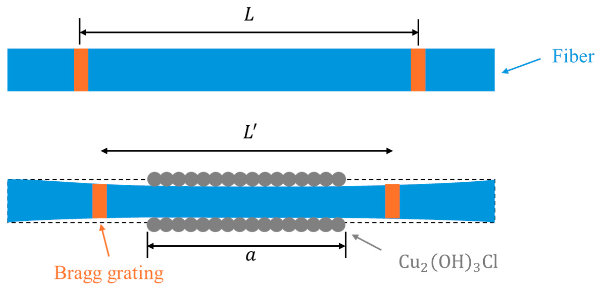
The corrosion mechanism is roughly divided into two stages. In the early stages of corrosion, as shown in Figure 9, corrosion products begin to form on the copper surface over time, generating bottom-up support forces that gradually lift the laid optical fiber upward by $h$. This causes the grating to stretch by $\Delta L=L_0^{\prime }-L_0$, resulting in a red shift $\Delta {\lambda }_B$ of the sensor’s Bragg wavelength [15]. Therefore,

$$h={\displaystyle \frac{1}{2}}\sqrt{L^2-L_0^2}={\displaystyle \frac{1}{2}}\sqrt{\mathsf{\Delta }L\left(\mathsf{\Delta }L+2L_0\right)}={\displaystyle \frac{1}{2}}{L}_0\sqrt{\alpha \Delta {\lambda }_B\left(\alpha \Delta {\lambda }_B+2\right)}$$

(16)

where $\alpha =1/{\lambda }_B\left(1-P_e\right)$.

Figure 9. Corrosion products on the copper surface lift the optical fiber by $h$. (The dotted line represents the initial shape of the optical fiber.)

During the mid-to-late stages of corrosion, as time progresses, more corrosion products appear on the copper surface. These corrosion product particles, driven by van der Waals forces, cover the fiber from all directions, exerting an overall pressure on the fiber. This causes relative compression $\Delta L^{\prime }=L-L^{\prime }$ in the grating, resulting in a blue shift $\Delta {\lambda }_B^{\prime }$ of the sensor’s Bragg wavelength, as shown in Figure 10. $\Delta L^{\prime }$ can be roughly expressed as [36]

$$\Delta L^{\prime }={\displaystyle \frac{\left(1-2\nu \right)\left(1+\nu \right)}{E}}pa$$

(17)

where $\nu$ is the Poisson’s ratio of the fiber, $E$ is the Young’s modulus, $p$ is the adhesion pressure, and $a$ is the length of the adhesion area. Therefore,

$$\Delta {\lambda }_B^{\prime }={\lambda }_B\left(1-P_e\right){\displaystyle \frac{\mathsf{\Delta }{L}^{\prime }}{L}}$$

(18)

Figure 10. Adhesion of corrosion products leads to fiber compression.

Substituting $\nu =0.17,E=73.1\mathrm{G}\mathrm{P}\mathrm{a},p=3.98\mathrm{M}\mathrm{P}\mathrm{a},a=0.4\mathrm{m},{\lambda }_B=1550\mathrm{n}\mathrm{m},P_e=0.22$ into Equations (17) and (18) yields $\Delta {\lambda }_B^{\prime }\approx 20\mathrm{p}\mathrm{m}$. This is of the same order of magnitude as the wavelength drift shown in Figure 5, indicating that the van der Waals forces between the corrosion products and the optical fiber are one of the primary factors causing the wavelength drift.

Due to the short effective range $h$ of van der Waals forces ($h\approx 5\mathsf{\mu }\mathrm{m}$), Equation (12) holds only when $D\le h$. When $D>h$, the corrosion particles outside the effective range interact minimally with the substrate.

5. Conclusions

This paper presents an experimental investigation into the effect of localized corrosion on the sensing signal between a corroded Cu substrate and optical fiber, employing discrete FBG sensors to monitor corrosion severity. The systematic strategy developed in this study yields several crucial conclusions. The corrosion products consist of loose or dense collections of micrometer/nanometer-sized particles in a crystalline state. And the corrosion products are composed of a multi-component crystal structure. FBG sensors exhibited the highlighted response by the wavelength shift in the monitoring points and the ability to identify the corrosion process in real time. Finally, according to contact mechanics theory, a mechanical-dependent corrosion monitoring model is proposed to investigate the influence of the corrosion products on the mechanical behavior of optical fiber.

References

- Zhang, J.W.; Wei, C. Materials analysis of traditional Chinese copper halls using XRF and GIS: Kunming Copper Hall as a case study. Front. Archit. Res. 2013, 2, 74–84. [Google Scholar] [CrossRef] [Scilit]
- Yan, J.; Hu, H.T.; Lu, H.L.; Yin, Y.C.; Bu, Y.F.; Lu, Q.Z. Experimental Study on the Influence of Cross-Section Type of Marine Cable Conductors on the Bending Performance. China Ocean. Eng. 2022, 36, 629–637. [Google Scholar] [CrossRef] [Scilit]
- King, F.; Lilja, C.; Vähänen, M. Progress in the understanding of the long-term corrosion behaviour of copper canisters. J. Nucl. Mater. 2013, 438, 228–237. [Google Scholar] [CrossRef] [Scilit]
- Mansfeld, F.; Liu, G.; Little, B.J. The corrosion behavior of copper-alloys, stainless-steels and titanium in seawater. Corros. Sci. 1994, 36, 2063–2095. [Google Scholar] [CrossRef] [Scilit]
- Carlesi, C.; Harris, R.C.; Abbott, A.P.; Jenkin, G.R.T. Chemical Dissolution of Chalcopyrite Concentrate in Choline Chloride Ethylene Glycol Deep Eutectic Solvent. Minerals 2022, 12, 65. [Google Scholar] [CrossRef] [Scilit]
- Mattsson, E. Corrosion of copper and brass: Practical experience in relation to basic data. Br. Corros. J. 1980, 15, 6–13. [Google Scholar] [CrossRef] [Scilit]
- Shinato, K.W.; Zewde, A.A.; Jin, Y. Corrosion protection of copper and copper alloys in different corrosive medium using environmentally friendly corrosion inhibitors. Corros. Rev. 2020, 38, 101–109. [Google Scholar] [CrossRef] [Scilit]
- Feng, Y.; Siow, K.S.; Teo, W.K.; Tan, K.L.; Hsieh, A.K. Corrosion mechanisms and products of copper in aqueous solutions at various pH values. Corrosion 1997, 53, 389–398. [Google Scholar] [CrossRef] [Scilit]
- Drach, A.; Tsukrov, I.; DeCew, J.; Aufrecht, J.; Grohbauer, A.; Hofmann, U. Field studies of corrosion behaviour of copper alloys in natural seawater. Corros. Sci. 2013, 76, 453–464. [Google Scholar] [CrossRef] [Scilit]
- Parvizi, M.S.; Aladjem, A.; Castle, J.E. Behaviour of 90–10 cupronickel in sea water. Int. Mater. Rev. 1988, 33, 169–200. [Google Scholar] [CrossRef]
- Strandberg, H.; Johansson, L.G. Some aspects of the atmospheric corrosion of copper in the presence of sodium chloride. J. Electrochem. Soc. 1998, 145, 1093–1100. [Google Scholar] [CrossRef] [Scilit]
- Hou, B.R.; Li, X.G.; Ma, X.M.; Du, C.W.; Zhang, D.W.; Zheng, M.; Xu, W.C.; Lu, D.Z.; Ma, F.B. The cost of corrosion in China. npj Mater. Degrad. 2017, 1, 4. [Google Scholar] [CrossRef] [Scilit]
- Boulay, N.; Edwards, M. Role of temperature, chlorine, and organic matter in copper corrosion by-product release in soft water. Water Res. 2001, 35, 683–690. [Google Scholar] [CrossRef] [Scilit]
- Feng, Y.; Teo, W.K.; Siow, K.S.; Hsieh, A.K. The corrosion behaviour of copper in neutral tap water. Part I: Corrosion mechanisms. Corros. Sci. 1996, 38, 369–385. [Google Scholar] [CrossRef] [Scilit]
- Xu, L.Y.; Shi, S.M.; Huang, Y.; Yan, F.; Yang, X.Y.; Bao, Y. Corrosion monitoring and assessment of steel under impact loads using discrete and distributed fiber optic sensors. Opt. Laser Technol. 2024, 174, 110553. [Google Scholar] [CrossRef] [Scilit]
- Szakálos, P.; Hultquist, G.; Wikmark, G. Corrosion of copper by water. Electrochem. Solid-State Lett. 2007, 10, C63–C67. [Google Scholar] [CrossRef] [Scilit]
- Lu, P.; Lalam, N.; Badar, M.; Liu, B.; Chorpening, B.T.; Buric, M.P.; Ohodnicki, P.R. Distributed optical fiber sensing: Review and perspective. Appl. Phys. Rev. 2019, 6, 041302. [Google Scholar] [CrossRef] [Scilit]
- Bao, Y.; Huang, Y.; Hoehler, M.S.; Chen, G.D. Review of fiber optic sensors for structural fire engineering. Sensors 2019, 19, 877. [Google Scholar] [CrossRef] [Scilit]
- Gao, J.Q.; Wu, J.; Li, J.; Zhao, X.M. Monitoring of corrosion in reinforced concrete structure using Bragg grating sensing. Ndt E Int. 2011, 44, 202–205. [Google Scholar] [CrossRef] [Scilit]
- Abu Hassan, M.R.; Abu Bakar, M.H.; Dambul, K.; Adikan, F.R.M. Optical-based sensors for monitoring corrosion of reinforcement rebar via an etched cladding Bragg grating. Sensors 2012, 12, 15820–15826. [Google Scholar] [CrossRef] [Scilit]
- Wang, Y.L.; Shi, B.; Zhang, T.L.; Zhu, H.H.; Sun, Q. Introduction to an FBG-based inclinometer and its application to landslide monitoring. J. Civ. Struct. Health Monit. 2015, 5, 645–653. [Google Scholar] [CrossRef] [Scilit]
- Al Handawi, K.; Vahdati, N.; Rostron, P.; Lawand, L.; Shiryayev, O. Strain based FBG sensor for real-time corrosion rate monitoring in pre-stressed structures. Sens. Actuators B Chem. 2016, 236, 276–285. [Google Scholar] [CrossRef] [Scilit]
- Sousa, I.; Pereira, L.; Mesquita, E.; Sousa, V.; Araújo, W.S.; Carbral, A.; Albert, N.; Varum, H.; Antunes, P. Sensing System Based on FBG for Corrosion Monitoring in Metallic Structures. Sensors 2022, 22, 5947. [Google Scholar] [CrossRef] [Scilit] [PubMed]
- Tan, X.; Fan, L.; Huang, Y.; Bao, Y. Detection, visualization, quantification, and warning of pipe corrosion using distributed fiber optic sensors. Autom. Constr. 2021, 132, 103953. [Google Scholar] [CrossRef] [Scilit]
- Xu, L.Y.; Shi, S.M.; Yan, F.; Huang, Y.; Bao, Y. Experimental study on combined effect of mechanical loads and corrosion using tube-packaged long-gauge fiber Bragg grating sensors. Struct. Health Monit. 2023, 22, 3985–4004. [Google Scholar] [CrossRef] [Scilit]
- Liu, X.B.; Liang, L.; Jiang, K.; Xu, G. Sensitivity-enhanced fiber Bragg grating pressure sensor based on a diaphragm and hinge-lever structure. IEEE Sens. J. 2020, 21, 9155–9164. [Google Scholar] [CrossRef] [Scilit]
- Liu, P.H.; Jiang, W.H.; Zhao, Z.J.; Yu, X.B.; Fu, Y.M.; Sun, D.D.; Chen, P.; Ma, J. Crack monitoring of tensile members in FBG sensing technology considering the strain redistribution of aluminium alloy substrates. Opt. Express 2025, 33, 43186. [Google Scholar] [CrossRef] [Scilit]
- Wang, Z.G.; Hai, C.; Jiang, J.; Lan, X.S.; Du, C.W.; Li, X.G. Corrosion behavior of Q235 steels in atmosphere at Deyang District for one Year. J. Chin. Soc. Corros. Prot. 2021, 41, 871–876. [Google Scholar]
- Myung, Y.; Jang, D.M.; Sung, T.K.; Sohn, Y.J.; Jung, G.B.; Cho, Y.J.; Kim, H.S.; Park, J. Composition-tuned ZnO−CdSSe core−shell nanowire arrays. ACS Nano 2010, 4, 3789–3800. [Google Scholar] [CrossRef] [Scilit]
- Li, Y.; Wei, X.Y.; Liu, Q.Y.; Zang, D.M.; You, R. Visible light-activated room temperature NO2 gas sensing based on the In2O3@ZnO heterostructure with a hollow microtube structure. ACS Sens. 2024, 9, 3741–3753. [Google Scholar] [CrossRef] [Scilit]
- Scott, D.A. Bronze disease: A review of some chemical problems and the role of relative humidity. J. Am. Inst. Conserv. 1990, 29, 193–206. [Google Scholar] [CrossRef]
- Doménech-Carbó, A.; Doménech-Carbó, M.T.; Costa, V. Electrochemical Basis of Corrosion of Cultural Objects, 1st ed.; Springer: Berlin/Heidelberg, Germany, 2009; pp. 123–134. [Google Scholar]
- Wang, H.P.; Dai, J.G.; Wang, X.Z. Improved temperature compensation of fiber Bragg grating-based sensors applied to structures under different loading conditions. Opt. Fiber Technol. 2021, 63, 102506. [Google Scholar] [CrossRef] [Scilit]
- Hamaker, H.C. The london-van der waals attraction between spherical particles. Phys. IV 1937, 10, 1058–1072. [Google Scholar] [CrossRef] [Scilit]
- Hideyuki, T.; Takashi, M.; Tatsuya, S.; Ryo, M.; Kenta, H. Method for the Calculation of the Hamaker Constants of Organic Materials by the Lifshitz Macroscopic Approach with Density Functional Theory. J. Phys. Chem. A 2019, 40, 8726–8733. [Google Scholar] [CrossRef] [Scilit]
- Johnson, K.L. Contact Mechanics; Cambridge University Press: Cambridge, UK, 1985. [Google Scholar]
Disclaimer/Publisher’s Note: The statements, opinions and data contained in all publications are solely those of the individual author(s) and contributor(s) and not of MDPI and/or the editor(s). MDPI and/or the editor(s) disclaim responsibility for any injury to people or property resulting from any ideas, methods, instructions or products referred to in the content. |
© 2026 by the authors. Licensee MDPI, Basel, Switzerland. This article is an open access article distributed under the terms and conditions of the Creative Commons Attribution (CC BY) license.