Neural Network Regression Structural Hyperparameter Selection Using Reconstruction Error Minimization (REM)

Abstract

Structural hyperparameter selection (HPS) in neural network (NN) regression faces two critical, computationally expensive barriers: the mandatory splitting of datasets for validation, which significantly impairs sample efficiency, and the inability of conventional metrics (like Data MSE) to decouple true modeling error from detrimental output noise, leading to suboptimal architectural complexity and overfitting. To resolve these systemic limitations, we propose the Reconstruction Error Minimization for Hyperparameter Selection (REM-HPS) framework, a novel, non-Bayesian approach grounded in statistical learning theory. REM-HPS fundamentally shifts the optimization objective by minimizing the Reconstruction Mean Squared Error (MSE), which precisely isolates and measures the model’s intrinsic ability to recover the underlying noise-free function. Since this target error is typically inaccessible, the framework employs the observable Data MSE (validation error) to construct a reliable, probabilistic estimate, yielding a deterministic and noise-aware selection criterion. REM-HPS utilizes a deterministic structural hyperparameter selection criterion that removes randomness due to validation data splitting, while remaining compatible with standard stochastic training procedures. This strategy allows for the use of the entire dataset for training, eliminating the need for explicit data splitting or the introduction of tuning-intensive regularization hyperparameters. Rigorous empirical validation demonstrates that REM-HPS consistently selects significantly more compact architectures (minimal complexity) while achieving superior generalizability and estimation accuracy, particularly across varied Signal-to-Noise Ratios and data regimes. By providing an efficient and optimal selection metric, REM-HPS offers a transformative, resource-efficient alternative to structural HPS in modern data-driven systems.

1. Introduction

In the realm of machine learning and neural networks (NNs), a crucial distinction exists between parameters and hyperparameters in data-based modeling algorithms. Parameters, such as weights and biases within NNs, are learned directly from the data during training. In contrast, hyperparameters govern the model’s architecture, training process, or regularization strategies and are either set prior to the modeling or selected through procedures such as grid search. Their values significantly influence generalization performance and model effectiveness, especially in regression tasks.

Hyperparameters in neural networks can be broadly grouped into two categories: structural and training hyperparameters. Structural hyperparameters define the architecture of the model. These hyperparameters include the number of layers, neurons per layer, and the type of activation functions. They determine the model’s inherent capacity to represent complex functions. Training hyperparameters control the learning process and optimization dynamics. They encompass learning rate, batch size, number of epochs, optimizer choice, and regularization techniques such as dropout rate and L1/L2 penalty coefficients. Although regularization affects the model’s behavior, it is applied during training and adjusted in conjunction with other learning parameters to improve generalization and reduce overfitting. The focus of this work is exclusively on structural hyperparameter selection (HPS).

HPS has attracted considerable attention, with methods spanning Bayesian and non-Bayesian paradigms. Bayesian methods offer a probabilistic treatment of uncertainty in hyperparameter selection and can be categorized into several groups. In approaches with model parameter uncertainty, such as probabilistic PCA [1] and Bayesian neural networks (BNNs) [2,3,4], the focus is often on latent variables or weight distributions while overlooking the role of output noise in structural hyperparameter optimization. Hyperparameter-induced uncertainty methods [5] aim to capture model uncertainty more directly but typically introduce additional layers of mathematical and computational complexity. Search-based Bayesian optimization frameworks, such as the CASOH algorithm [6], integrate Markov Chain Monte Carlo with uniform sampling to improve search efficiency but remain resource-intensive. Empirical studies [7] further demonstrate that hyperparameter choices affect not only predictive accuracy but also critical performance metrics such as latency and model size, underscoring the need for methods that are both accurate and computationally efficient.

On the other hand, many popular techniques in non-Bayesian settings rely on search strategies such as grid search [8,9], adaptive grid search [10], and random search [11], which, while conceptually simple, quickly become computationally infeasible as the hyperparameter space expands.

Other approaches aim to automate selection using statistical modeling [12], gradient-based approximations [13,14], reinforcement learning methods [13,15], genetic algorithms [16,17], random and grid search, and weighted random search strategies [18]. Gradient-based methods can avoid explicit data splitting [19] but scale poorly with network size, while implicit regularization via stochastic gradient descent (SGD) can influence learning trajectories without explicitly modeling output noise [20]. Meta-learning can warm-start the search process [21], but its effectiveness depends heavily on the availability of similar prior experiments, limiting generalization to novel tasks. Analytic methods such as alternating least-squares training of two-layer ReLU networks [22] show promise in certain settings but lack theoretical guarantees for global optimality and are restricted to specific architectures. Data augmentation techniques generate synthetic training examples through label-preserving transformations to expand the size and diversity of the training set [23]; however, these methods require a policy management strategy that introduces an additional layer of complexity. Some HPS issues have been partially addressed by methods that utilize partial data information, such as greedy feature selection and approaches that incorporate constraints on the cost function [24,25,26,27]. However, these methods typically rely on some form of prior data awareness. In this work, while we acknowledge similar fundamental flaws in the HPS procedure, we consider the general HPS question without requiring prior knowledge of the available underlying structure of the data.

Consequently, validation-based approaches remain among the most widely used for regression tasks [4] and HPS in deep neural networks [28,29] due to their generality and empirical reliability. However, they require multiple data partitions, which increases computational cost and introduces randomness. These issues are only partially mitigated by k-fold cross-validation and its greedy versions [30,31]. Alternatives that avoid data splitting, such as discretized-space selection using actively sampled datasets [32], achieve logarithmic complexity under adversarial noise assumptions, but still demand strong prior knowledge of the noise distribution and careful space-discretization conditions rarely satisfied in practice. Strategies for HPS in neural networks, for these existing approaches, focus on choosing architectural configurations that optimize generalization performance while mitigating overfitting [33,34].

The appropriate selection of a loss function also plays a crucial role in the HPS process. Regularization-based methods address model complexity either through soft regularization, adding penalty terms to the base loss function, or hard regularization techniques such as dropout, which randomly deactivate neurons during training to prevent co-adaptation. The choice of base loss function is independent of these regularization methods. Common examples include Mean Squared Error (MSE), which is statistically efficient under Gaussian noise but sensitive to outliers; mean absolute error (MAE), which is more robust to outliers but less smooth [35,36]; and Huber loss, which blends the two by behaving quadratically for small errors and linearly beyond a threshold [37,38]. MAE and Huber loss have been used in training and validation to improve robustness against outliers in various applications, such as regression modeling [35,36,37].

Validation-based HPS methods evaluate candidate hyperparameter configurations using holdout validation sets or cross-validation sets and various types of loss functions. The selected validation metric directly guides structural choices; the loss function defining the optimization objective, the regularization constraining model complexity, and the validation step assessing generalization represent three distinct yet complementary components in the HPS process. Regularization techniques introduce additional hyperparameters, such as penalty coefficients, which themselves require additional tuning and may complicate the optimization process. Therefore, these methods are excluded from consideration in this work. Validation-based methods, on the contrary, require splitting the data into holdout or cross-validation sets, introducing additional randomness that is typically mitigated through k-fold validation. Since handling outliers is not the focus of this study, we adopt the MSE loss function for its simplicity and statistical efficiency under Gaussian noise.

Alternatively, Bayesian evidence optimization selects hyperparameters by maximizing the marginal likelihood after integrating out the network weights [39]. In principle, this results in a probabilistic trade-off between data fit and model complexity, representing an Occam’s razor effect. However, for nonlinear and overparameterized neural networks, the marginal likelihood is intractable and must be approximated, which can heavily bias the evidence landscape and lead to unstable or misleading hyperparameter choices. The approach is also highly sensitive to the choice of weight priors and handles discrete architectural changes (e.g., number of layers or neurons) poorly, since each architecture alters the parameter dimension and complicates evidence computation. These limitations restrict Bayesian evidence optimization as a practical tool for structural hyperparameter selection in nonlinear NN regression and motivate alternatives such as REM-HPS that explicitly handle output noise while remaining computationally tractable. Moreover, it is important to note that such Bayesian optimization frameworks do not change the underlying selection criterion; in practice, they typically optimize the same validation or cross-validation MSE as conventional search strategies, improving the efficiency of the search in hyperparameter space but not the quality of the metric itself.

This paper focuses exclusively on structural hyperparameter selection (HPS) in regression tasks under the non-Bayesian paradigm. Although existing approaches have advanced the field, they face common drawbacks when applied to structural HPS: excessive computational demands, reliance on strong prior assumptions, sensitivity to data partitioning strategies, and limited treatment of output noise. In contrast, the proposed Reconstruction Error Minimization for Hyperparameter Selection (REM-HPS) framework avoids explicit regularization and bypasses validation-based data splitting. Rather than relying on Data MSE validation to guide hyperparameter selection, we propose an alternative loss function defined as the Reconstruction MSE criterion, which directly evaluates the model’s ability to reconstruct training data and serves as a deterministic metric for structural hyperparameter optimization. This error has attracted attention in areas such as image denoising and feature extraction [40]. However, in these methods, the reconstruction error is available. The significant challenge addressed in this work is that this crucial error is usually unavailable. The proposed method employs the validation MSE (denoted as Data MSE in this work) to provide a reliable probabilistic estimate of the target Reconstruction MSE, offering a simpler yet more robust alternative for structural hyperparameter tuning. As summarized in Table 1, REM-HPS offers a theoretically grounded, efficient, and noise-aware alternative to conventional validation-based approaches.

Our proposed approach is inspired by the introduction of the reconstruction error for parametric modeling, established as a new information-theoretic framework based on statistical learning theory [41]. Using the available Data MSE, which conventionally uses the validation MSE in existing methods, to approximate the desired Reconstruction MSE has proven to be an effective hyperparameter selection strategy. This strategy has been successfully applied in several domains, including system modeling and time-delay estimation [42]; thresholding, source separation, and multimodal source selection localization [43,44]; hyperparameter selection for autoregressive moving average (ARMA) modeling [45]; and polynomial regression [46]. This body of work demonstrates the versatility and effectiveness of MSE-based hyperparameter criteria in various estimation and learning tasks. Our method extends this principle to neural network regression by defining a loss function that directly accounts for the additive noise in the target output, a key factor contributing to problems in existing hyperparameter selection methods. Empirical simulations and analysis demonstrate the effectiveness of REM-HPS in improving model accuracy and sample efficiency by eliminating data splitting and addressing the critical issue of overfitting. The results highlight the advantages of the proposed method over validation-based approaches in estimating accuracy and in minimizing the desired MSE, achieved by selecting fewer hyperparameters simultaneously. The proposed method selects hyperparameters while efficiently considering the role of the SNR, thus avoiding overfitting more effectively than competing approaches. While the Universal Approximation Theorem guarantees the existence of a neural network capable of approximating the underlying function, the proposed approach provides a practical mechanism for selecting a minimally sufficient architecture that avoids overfitting in the presence of noisy data.

Table 1. Comparison of structural hyperparameter optimization methods in neural network regression.

Method	Requires Data Split	Efficiency	Adds New Hyperparameters	Loss Function Type
REM-HPS (proposed)	No	High	No	Reconstruction MSE
k-Fold Cross-Validation	Yes	Low	No (Except:value of k)	Data MSE (Validation)
Bayesian Optimization [34,47]	Yes	Medium	Yes	Data MSE (Surrogate Model)
Gradient-Based Methods [12]	No	Medium	Yes	Data MSE (Validation)
Meta-Learning [21]	Varies	Medium	Yes	Data MSE (Validation on Prior Tasks)
Regularization ($L1/L2$, Dropout)	No	High	Yes	Data MSE + Penalty Term

Table 1. Comparison of structural hyperparameter optimization methods in neural network regression.

Method	Requires Data Split	Efficiency	Adds New Hyperparameters	Loss Function Type
REM-HPS (proposed)	No	High	No	Reconstruction MSE
k-Fold Cross-Validation	Yes	Low	No (Except:value of k)	Data MSE (Validation)
Bayesian Optimization [34,47]	Yes	Medium	Yes	Data MSE (Surrogate Model)
Gradient-Based Methods [12]	No	Medium	Yes	Data MSE (Validation)
Meta-Learning [21]	Varies	Medium	Yes	Data MSE (Validation on Prior Tasks)
Regularization ($L1/L2$, Dropout)	No	High	Yes	Data MSE + Penalty Term

2. Neural Network Regression Modeling

Here, the two steps of the NN regression modeling are summarized. The first step is parameter estimation, which consists of estimating the weights. The second step is the selection of the structural hyperparameters. These hyperparameters include modeling factors such as the number of layers, the number of neurons per layer, and the activation function.

2.1. Parametric Modeling: MSE-Based Learning in Neural Network Regression

If the data can be generated by a parametric model with p parameters, then for the observed input–output pairs of length n, denoted by (${\mathbf{x}}_{\mathbf{n}},{\mathbf{y}}_{\mathbf{n}}$), we have

$${\mathcal{H}}_p:{\mathbf{y}}_{\mathbf{n}}=f({\mathit{\theta }}_p,{\mathbf{x}}_{\mathbf{n}})$$

(1)

For a given hypothesis class, parameter estimation involves minimizing a chosen loss function through empirical risk minimization to learn the parameter ${\theta }_p$ as follows:

$${\widehat{\mathit{\theta }}}_p=arg\underset{{\mathit{\theta }}_p\in {\mathcal{H}}_p}{min}\ell ({\mathit{\theta }}_p,{\mathbf{y}}_{\mathbf{n}},{\mathbf{x}}_{\mathbf{n}})$$

(2)

where ${\widehat{\theta }}_p$ denotes the estimated parameter. The loss function is usually in the form of Mean Squared Error (MSE), which is more commonly used than alternatives such as Mean Absolute Error (MAE) and R-squared in machine learning and mostly for regression or reconstruction tasks. Neural networks typically use the MSE loss function, which is differentiable and therefore suitable for optimization algorithms such as gradient descent.

2.2. Structural Hyperparameter Selection and Motivation

Hyperparameter tuning or selection occurs alongside the parameter estimation approach. In this step, the optimal number of parameters and their associated estimates are selected. The set of hyperparameter combinations is defined as

$$\mathcal{P}=[p_{min},p_{min+1},\dots ,p_{max}]$$

(3)

For hyperparameter tuning, a loss function is defined to evaluate the performance as the hyperparameter varies, with the goal of identifying an optimal value that avoids underfitting or overfitting the model:

$$HS\left(p\right)={\ell }_H({\widehat{\mathit{\theta }}}_p,{\mathbf{y}}_{\mathbf{n}},{\mathbf{x}}_{\mathbf{n}})$$

(4)

$$\widehat{p}=\underset{p\in \mathcal{P}}{argmin}HS\left(p\right)$$

(5)

where ${\ell }_H$ denotes the structural hyperparameter loss function. As noted earlier, complex loss functions defined for ${\ell }_H$ are often problem-specific regularization methods. These functions add complexity to the model [48] and are not the focus of this work. Using the MSE from the parameter estimation step in (2) as a loss function for hyperparameter selection presents challenges due to its tendency to decrease monotonically as model complexity increases, as shown by the maximum likelihood analysis. This often results in the selection of overly complex models. To overcome this issue, regularization methods propose alternative loss functions, which themselves introduce additional hyperparameters and computational complexity. These methods are not the focus of this work. On the other hand, in the validation and cross-validation methods, the data of length n is divided into a training set $n_T$ and a validation set $n_V$. Initially, $n_T$ is used for parameter estimation with fixed hyperparameters, followed by evaluation on $n_V$ to select the best hyperparameters based on the validation error. A significant issue is determining the optimal lengths of $n_T$ and $n_V$, which are often chosen by trial and error, affecting the convergence and precision of the model. Even with fixed lengths, variations in data subsets can affect the results. While k-fold cross-validation addresses some of these challenges by using multiple data splits, it also increases runtime, which may be undesirable.

This work is motivated by two key drawbacks in existing methods: (1) the hyperparameter selection loss function in (4), which takes the form of Data MSE. While regularization approaches introduce additional terms, validation methods focus on data error MSE, which, as previously described, tends to decrease as the dimensionality of the hyperparameters increases. However, retaining this loss function without added complexity leads to a second drawback in validation: (2) splitting the training data into separate training and validation sets. Motivated by these two issues, this work proposes using an alternative loss function that does not introduce additional hyperparameters and utilizes the available Data MSE without requiring data to be split into separate parts for hyperparameter selection. Consequently, the proposed REM-HPS method can converge to true parametric models using fewer data samples and with faster performance in online applications.

3. REM-HPS-Based Modeling: A Paradigm Shift in Hyperparameter Selection

The formulation described in the previous section, commonly used in machine learning models, including neural networks, usually disregards uncertainty and potential noise in the observed output data ${\mathbf{y}}_{\mathbf{n}}$, as shown below:

$${\mathbf{y}}_{\mathbf{n}}={\overline{\mathbf{y}}}_{\mathbf{n}}+{\mathit{\omega }}_{\mathbf{n}}$$

(6)

where noise-free ${\overline{\mathbf{y}}}_{\mathbf{n}}$ is a function of the input ${\mathbf{x}}_{\mathbf{n}}$ and can be modeled by a parametric structure with parameters $\theta$. Here, ${\mathit{\omega }}_{\mathit{n}}={[\mathit{\omega }\left(\mathbf{1}\right),\mathit{\omega }\left(\mathbf{2}\right),\dots ,\mathit{\omega }\left(\mathit{n}\right)]}^T$ denotes the additive white Gaussian noise with variance ${\sigma }_{\omega }^2$ that affects the observations. This noise term is independent of both the input ${\mathbf{x}}_{\mathbf{n}}$ and the model parameters $\theta$ and represents uncertainty in the measured output. There are three types of uncertainties that can be considered in this modeling procedure. The first type of uncertainty lies in the input, whether it has a probabilistic structure, represents a typical sample from its distribution, or exhibits skewness. These aspects are the focus of methods such as Probably Approximately Correct (PAC) learning [41]. Secondly, the parameter $\theta$ can be probabilistic, and issues related to its distribution and the role of stochastic parameters are addressed in work such as Bayesian PCA and Bayesian Neural Networks (BNNs). The third type of uncertainty is in the output and is not due to the input or parameter uncertainty, but rather takes the form of an exogenous additive noise term ${\mathit{\omega }}_{\mathit{n}}$, as shown in (6). This work focuses on the third case and lays the foundation for future integration with the first two types of uncertainty. REM-HPS directly incorporates output-noise statistics into hyperparameter selection, avoiding data splitting and providing a computationally efficient alternative to Bayesian approaches [41].

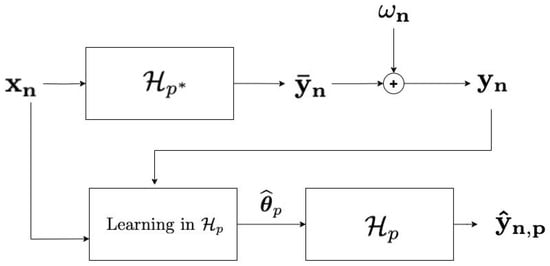
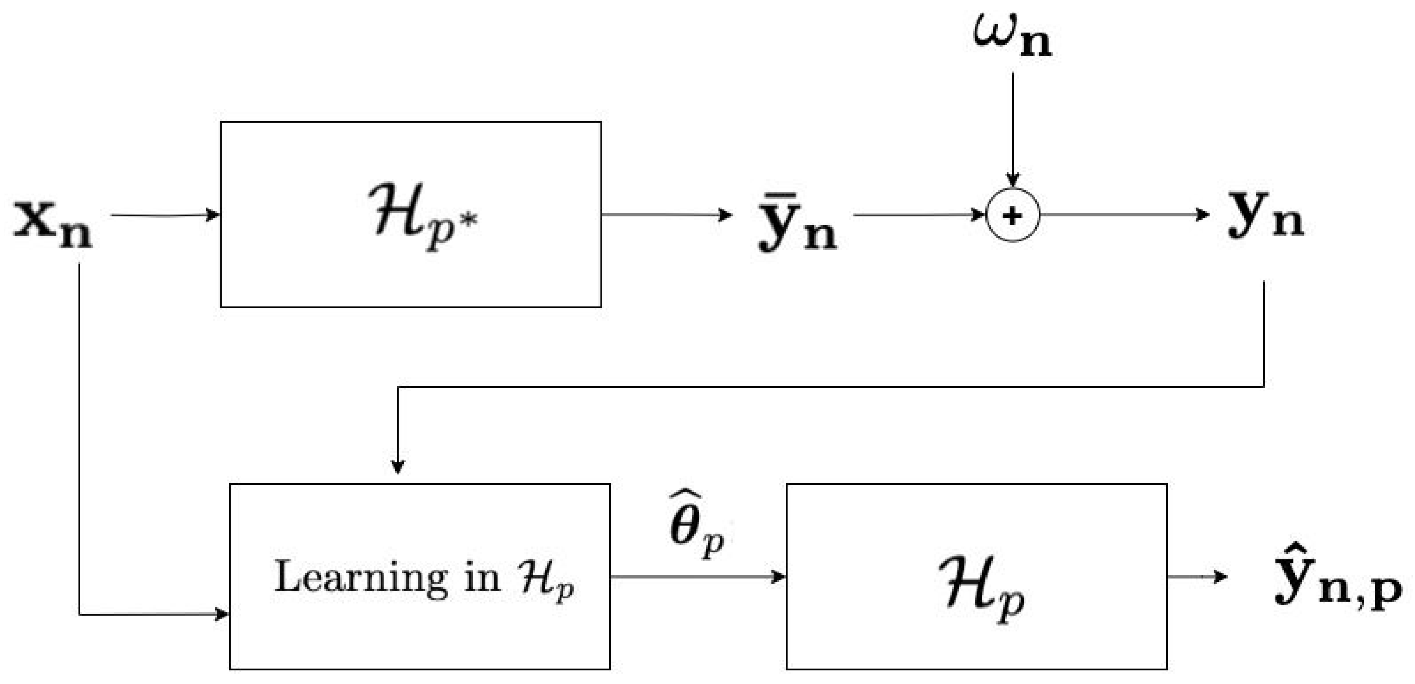
Figure 1 illustrates the parameter modeling step in the presence of additive output noise, assuming that the data was generated by a true hyperparameter structure, which is the focus of the present work. As the figure shows, the available output is a noisy version of the desired output ${\overline{\mathbf{y}}}_{\mathbf{n}}$, generated by the true hypothesis ${\mathcal{H}}_{p^{*}}$ with the true number of parameters $p^{*}$. The relation between ${\overline{\mathbf{y}}}_{\mathbf{n}}$, ${\mathbf{x}}_{\mathbf{n}}$ and ${{\mathit{\theta }}^{*}}_{p^{*}}$ is expressed as follows:

$${\mathcal{H}}_{p^{*}}^{*}:{\overline{\mathbf{y}}}_{\mathbf{n}}=f({{\mathit{\theta }}^{*}}_{p^{*}},{\mathbf{x}}_{\mathbf{n}})$$

(7)

where ${\theta }_{p^{*}}^{*}$ is the true parameter vector within the parameter space ${\theta }_{p^{*}}$ corresponding to the true model order $p^{*}$. In practical applications, the actual hypothesis class is often inaccessible, which means that the function $f({{\mathit{\theta }}^{*}}_{p^{*}},{\mathbf{x}}_{\mathbf{n}})$ is typically unknown, just as the noise-free output ${\overline{\mathbf{y}}}_{\mathbf{n}}$ is also unavailable.

Figure 1. Parametric modeling in the presence of additive output noise.

The structural hyperparameter selection relies on the parametric estimates of each competing hyperparameter $H_p$. The parameters in each $H_p$ are calculated using the MSE loss function as $\ell ({\mathit{\theta }}_p,{\mathbf{y}}_{\mathbf{n}},{\mathbf{x}}_{\mathbf{n}})$ in (2), defined as follows:

$$\begin{array}{c}\hfill {\displaystyle \ell ({\mathit{\theta }}_p,{\mathbf{y}}_{\mathbf{n}},{\mathbf{x}}_{\mathbf{n}})=X_{S_p}({\mathit{\theta }}_p,{\mathbf{y}}_{\mathbf{n}},{\mathbf{x}}_{\mathbf{n}})=\frac{1}{n}\sum _{i=1}^n{(y_n\left(i\right)-f({\mathit{\theta }}_p,x_n\left(i\right)))}^2}\end{array}$$

(8)

The parameter that minimizes this cost function is denoted by ${\widehat{\theta }}_p$. We refer to the loss function evaluated at this estimated parameter as the data error, denoted by $X_{S_p}$:

$${\displaystyle X_{S_p}({\widehat{\mathit{\theta }}}_p,{\mathbf{y}}_{\mathbf{n}},{\mathbf{x}}_{\mathbf{n}})=\frac{1}{n}\sum _{i=1}^n{(y_n\left(i\right)-{\widehat{y}}_{n,p}\left(i\right))}^2}$$

(9)

where ${\widehat{\mathbf{y}}}_{\mathbf{n},\mathbf{p}}$, shown in Figure 1, represents the estimated output generated using the assessed parameter ${\widehat{\mathit{\theta }}}_p$:

$${\widehat{\mathbf{y}}}_{\mathbf{n},\mathbf{p}}=f({\widehat{\mathit{\theta }}}_p,{\mathbf{x}}_{\mathbf{n}})$$

(10)

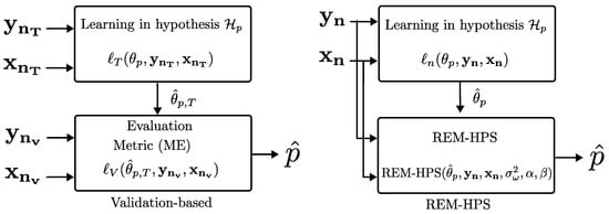
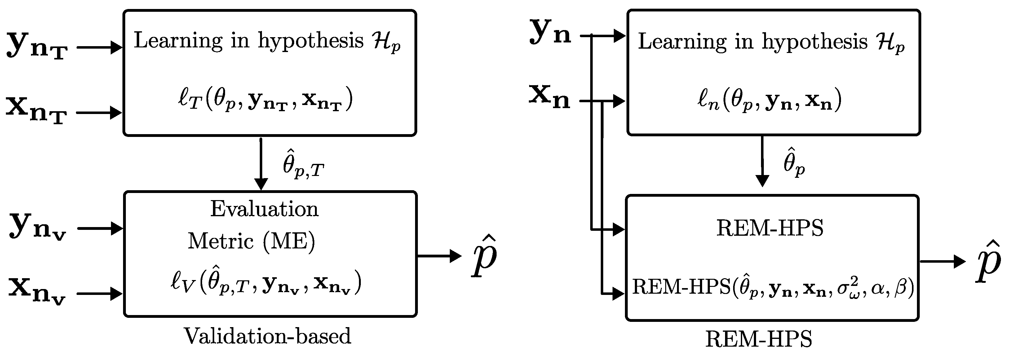
Figure 2, on the other hand, depicts the hyperparameter selection process for both validation-based methods and REM-HPS, the method proposed in this section. In this figure, the important structural hyperparameter loss functions are shown for both approaches.

Figure 2. Hyperparameter selection: Conventional validation-based method and the proposed REM-HPS.

Validation approaches

1.

Parametric modeling: Training data error

In validation approaches, the training subset is used for parameter estimation. Accordingly, in Figure 1, n is replaced by $n_T$, representing the length of the training dataset, a portion of the whole data of length n. Using the data error defined in (9), the parameter estimate is given by

$${\widehat{\mathit{\theta }}}_{p,T}=arg\underset{{\mathit{\theta }}_p\in {\mathcal{H}}_p}{min}{X}_{S_p}({\mathit{\theta }}_p,{\mathbf{y}}_{{\mathbf{n}}_{\mathbf{T}}},{\mathbf{x}}_{{\mathbf{n}}_{\mathbf{T}}})$$

(11)

2.

Hyperparameter selection: Validating data error

In this approach, the hyperparameter loss function in (4) is the same as the parameter loss function, data error, but is evaluated on the validating dataset of length $n_V$, where $n=n_T+n_V$:

$${\ell }_H^V({\widehat{\mathit{\theta }}}_{p,T},{\mathbf{y}}_{\mathbf{n}},{\mathbf{x}}_{\mathbf{n}})=X_{S_p}({\widehat{\mathit{\theta }}}_{p,T},{\mathbf{y}}_{{\mathbf{n}}_{\mathbf{V}}},{\mathbf{x}}_{{\mathbf{n}}_{\mathbf{V}}})$$

(12)

REM-HPS

1.

Parametric modeling: Data error

In REM-HPS, the parameters within each hyperparameter class are calculated using the entire dataset of length n. Using the data error defined in (9) the parameter estimate is

$${\widehat{\mathit{\theta }}}_p=arg\underset{{\mathit{\theta }}_p\in {\mathcal{H}}_p}{min}{X}_{S_p}({\mathit{\theta }}_p,{\mathbf{y}}_{\mathbf{n}},{\mathbf{x}}_{\mathbf{n}})$$

(13)

2.

Hyperparametric selection: Reconstruction error

In this work, we propose the following cost function as the hyperparameter structural loss function in (4):

$$\begin{array}{c}\hfill {\displaystyle Z_{S_p}({\widehat{\mathit{\theta }}}_{\mathbf{p}},{\mathbf{y}}_{\mathbf{n}},{\mathbf{x}}_{\mathbf{n}})=\frac{1}{n}\sum _{i=1}^n{({\overline{y}}_n\left(i\right)-f({\widehat{\mathit{\theta }}}_{\mathbf{p}},x_n\left(i\right)))}^2}\end{array}$$

(14)

This metric, referred to as the reconstruction error, serves as the hyperparameter loss function in the proposed approach:

$$\begin{array}{c}\hfill {\ell }_H^{REM}({\widehat{\mathit{\theta }}}_p,{\mathbf{y}}_{\mathbf{n}},{\mathbf{x}}_{\mathbf{n}})=Z_{S_p}({\widehat{\mathit{\theta }}}_{\mathbf{p}},{\mathbf{y}}_{\mathbf{n}},{\mathbf{x}}_{\mathbf{n}})\end{array}$$

(15)

The proposed method, known as Reconstruction Error Minimization Hyperparameter Selection (REM-HPS), eliminates the traditional requirement of splitting data into separate training and validation sets, offering a more holistic and efficient approach to utilizing data in the hyperparameter optimization process. This approach not only streamlines the modeling process but also addresses key challenges such as data sparsity and overfitting, which are common in conventional validation-based methods.

3.1. Estimating the Reconstruction Error Using the Data Error

The desired cost function, expressed as the reconstruction error in (14), is not accessible because the noiseless data ${\overline{\mathbf{y}}}_{\mathbf{n}}$ are themselves unavailable. In [41,42], a novel approach is introduced that uses the available data error in (9) to provide probabilistic bounds on the reconstruction error. The worst-case probabilistic upper bound is denoted as $\overline{Z_{S_p}}\left(X_{S_p}\right)$:

$$\begin{array}{c}\hfill Z_{S_p}({\widehat{\mathit{\theta }}}_{\mathit{p}},{\mathbf{y}}_{\mathbf{n}},{\mathbf{x}}_{\mathbf{n}})\le \overline{Z_{S_p}}(X_{S_p}({\widehat{\mathit{\theta }}}_{\mathit{p}},{\mathbf{y}}_{\mathbf{n}},{\mathbf{x}}_{\mathbf{n}}),{\sigma }_{\omega }^2,{\theta }_p,{\mathbb{P}}_{\alpha },{\mathbb{P}}_{\beta })\end{array}$$

(16)

This upper bound is a function of the data error, the noise variance ${\sigma }_w^2$, and the validation and confidence probabilities ${\mathbb{P}}_{\alpha }$ and ${\mathbb{P}}_{\beta }$. Details on utilizing the observed data, and thus the available data error $X_{S_p}$ from (9), as well as estimating the noise variance ${\sigma }_w^2$, are provided in [41,42]. The full calculation for this scenario is provided in Appendix A. Minimizing the upper bound of the reconstruction error $\overline{Z_{S_p}}$ in (16) leads to an estimate of the hyperparameter $\widehat{p}$ from the candidate hyperparameter set $\mathcal{P}$ defined in (3):

$$\begin{array}{c}\hfill {\widehat{p}}_{REM}=\underset{p\in \mathcal{P}}{argmin}\overline{Z_{S_p}}(X_{S_p}({\widehat{\mathit{\theta }}}_{\mathit{p}},{\mathbf{y}}_{\mathbf{n}},{\mathbf{x}}_{\mathbf{n}}),{\sigma }_{\omega }^2,\alpha ,\beta )\end{array}$$

(17)

The upper bound is a function of the validation and confidence probabilities, which can be selected using the $3\sigma$ rule, corresponding to a confidence level of 99.73% [41], and is also adopted for the following simulation section. This calculation is proposed for linear parametric modeling with a least-squares solution. It can be extended to neural networks with ReLU activation functions. In this scenario, gradient-based methods yield a suboptimal solution for a nonconvex piecewise linear least-squares objective. The number of these piecewise linear least squares is determined by the number of neurons and by the number of layers. Conventional order selection approaches, such as the Akaike Information Criterion (AIC) and Bayesian Information Criterion (BIC), have been shown to be special cases of REM for particular choices of $\alpha$ and $\beta$ [42]. This fact explains the consistency of the BIC and the inconsistency of the AIC. In particular, AIC is $\overline{Z_{S_p}}\left(X_{S_p}\right)$ when $\alpha =\beta =0$. It is important to note that [46] demonstrates how validation-based approaches capture the AIC in the validation data error in (12) by splitting the data into training and validation sets. Algorithm 1 shows the pseudocode of the proposed REM-HPS method.

Algorithm 1 REM-HPS: Reconstruction Error Minimization for Structural Hyperparameter Selection.

Require:  Dataset $\mathcal{D}={\left\{(x\left(i\right),y\left(i\right))\right\}}_{i=1}^n$; candidate set $\mathcal{P}=\{p_{min},\dots ,p_{max}\}$; training algorithm $\mathrm{T}\mathrm{R}\mathrm{A}\mathrm{I}\mathrm{N}\_\mathrm{N}\mathrm{N}(\mathcal{D},p)$; probabilities $({\mathbb{P}}_{\alpha },{\mathbb{P}}_{\beta })$ (or equivalently $(\alpha ,\beta )$); upper bound $\overline{Z_{S_p}}(·)$ as in (16). Ensure:  Selected hyperparameter ${\widehat{p}}_{\mathrm{REM}}$ and trained parameters ${\widehat{\theta }}_{{\widehat{p}}_{\mathrm{REM}}}$.   1: Estimate output-noise variance ${\widehat{\sigma }}_{\omega }^2\leftarrow \mathrm{E}\mathrm{S}\mathrm{T}\mathrm{I}\mathrm{M}\mathrm{A}\mathrm{T}\mathrm{E}\mathrm{N}\mathrm{O}\mathrm{I}\mathrm{S}\mathrm{E}\mathrm{V}\mathrm{A}\mathrm{R}\left(\mathcal{D}\right)$.   2: for $p\in \mathcal{P}$ do   3:    Parametric modeling (use all data):   4:       ${\widehat{\theta }}_p\leftarrow \mathrm{T}\mathrm{R}\mathrm{A}\mathrm{I}\mathrm{N}\_\mathrm{N}\mathrm{N}(\mathcal{D},p)$ {minimizes $X_{S_p}$ in (8)}   5:    Compute Data Error:   6:       $X_{S_p}\left(p\right)\leftarrow {\displaystyle \frac{1}{n}}{\sum }_{i=1}^n{\left(y\left(i\right)-f({\widehat{\theta }}_p,x\left(i\right))\right)}^2$ {(9)}   7:    Compute REM score (upper bound on Reconstruction Error):   8:       ${\overline{Z}}_{S_p}\left(p\right)\leftarrow \overline{Z_{S_p}}\left(X_{S_p}\left(p\right),{\widehat{\sigma }}_{\omega }^2,{\theta }_p,{\mathbb{P}}_{\alpha },{\mathbb{P}}_{\beta }\right)$ {(16)}   9: end for 10: ${\mathcal{P}}^{★}\leftarrow arg{min}_{p\in \mathcal{P}}{\overline{Z}}_{S_p}\left(p\right)$. 11: ${\widehat{p}}_{\mathrm{REM}}\leftarrow min\{p:p\in {\mathcal{P}}^{★}\}$ {pick lowest complexity among ties} 12: return ${\widehat{p}}_{\mathrm{REM}},{\widehat{\theta }}_{{\widehat{p}}_{\mathrm{REM}}}$.

3.2. Computational Complexity

The training of a Multi-Layer Perceptron (MLP) with backpropagation exhibits symmetric computational complexity between its forward and backward passes. For an L-layer network, where layer i contains $m_i$ neurons, both passes have a time complexity of $\mathcal{O}\left({\sum }_{i=1}^L{m}_i\times m_{i-1}\right)$ per training example. This complexity arises from matrix–vector multiplications in $W^{\left(l\right)}{a}^{(l-1)}+b^{\left(l\right)}$ in each layer, where $W^l$ is the weight matrix of the lth layer, $a^{\left(l\right)}$ is the activation vector and $b^{\left(l\right)}$ is the bias vector. Therefore, for a dataset of n samples trained in e epochs, the total time complexity is $\mathcal{O}\left(e\times n\times {\sum }_{i=1}^L{m}_i\times m_{i-1}\right)=\mathcal{O}(e\times n\times W)$, where W represents the total weights in the network. The complexity scales linearly with the network depth and quadratically with the layer width [39]. Therefore, while the complexity of the proposed method is calculated for n samples, the computational complexity of the validation methods replaces n with $n_T$, and for k-fold cross-validation, it is k times that of the validation approach. This verifies the comparability of the computational complexity of the proposed method with the validation approaches.

4. Simulation Results

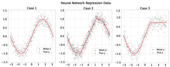
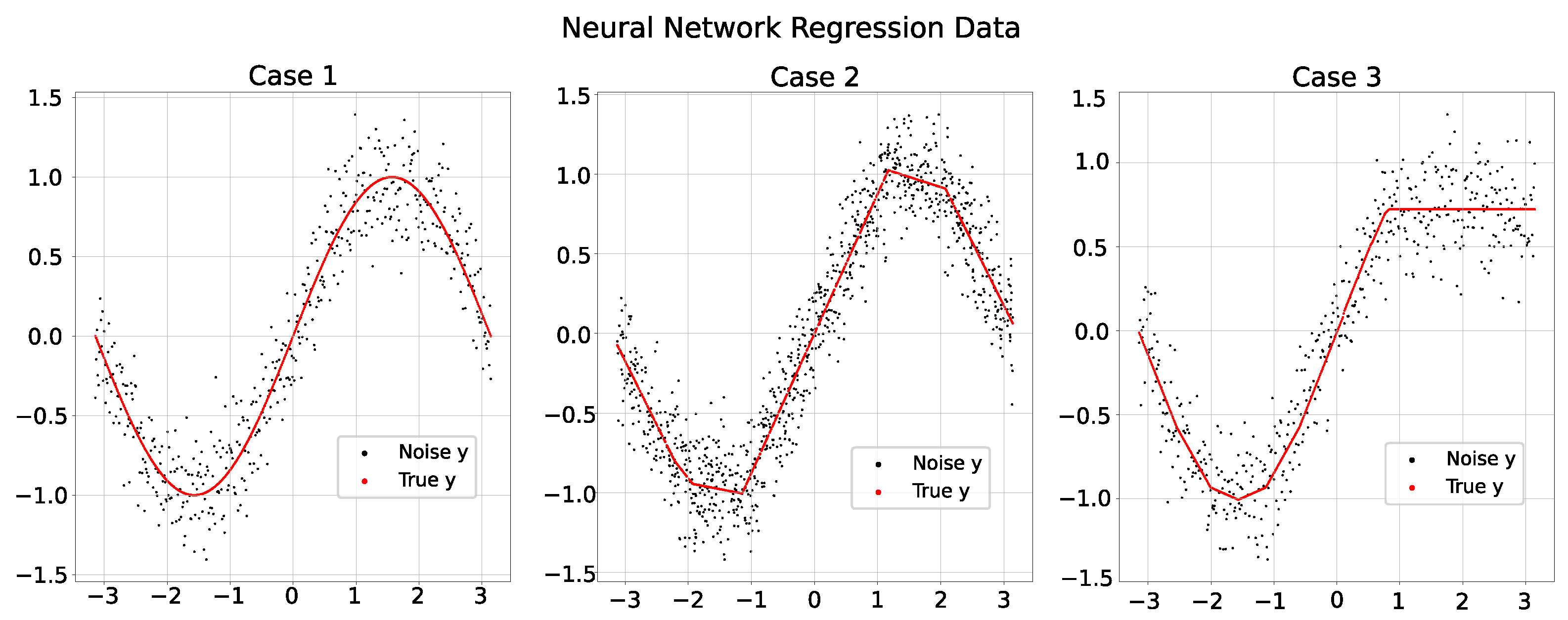
To illustrate some advantages of the proposed method, the approach is first examined over a simulated set of data, and then its performance is evaluated over a real-world dataset. Figure 3 illustrates three experimental cases designed to compare and evaluate hyperparameter selection methods. The noise-free target vector, $\overline{\mathbf{y}}$, is shown in red, while the available noisy target vector, $\mathbf{y}$, with the additive noise variance ${\sigma }_w^2=0.2$, is shown in black. The input vector ${\mathbf{x}}_{\mathbf{n}}$ is generated by uniform sampling from $-\pi$ to $\pi$.

Figure 3. Noise-free (in red) and noisy (in black) data with additive noise variance 0.2 in three cases. Case 1: Sine Wave; Case 2: 1-Layer, 5-Neuron NN Architecture; Case 3: 5-Layer, 3-Neuron-per-Layer NN Architecture.

(Case 1) 

Analytical Target: Sine Wave

The corresponding true target vector ${\overline{\mathbf{y}}}_{\mathbf{n}}$ is defined by ${\overline{\mathbf{y}}}_{\mathbf{n}}=sin\left({\mathbf{x}}_{\mathbf{n}}\right)$.

(Case 2) 

Shallow Neural Network Target: 1 Layer, 5 Neurons

The noise-free output target ${\overline{\mathbf{y}}}_{\mathbf{n}}$ is generated by passing the input ${\overline{\mathbf{x}}}_{\mathbf{n}}$ through a single-layer NN with five neurons ($L=1$ and $N=5$). The network uses a rectified linear unit (ReLU) activation function and has fixed predetermined weights.

(Case 3) 

Deep Neural Network Target: 5 Layer, 3 Neurons

The noise-free output target ${\overline{\mathbf{y}}}_{\mathbf{n}}$ is generated by passing the input through a five-layer NN with three neurons per layer ($L=5$ and $N=3$). As in the previous case, this network employs a ReLU activation function and fixed weights.

We conducted our experiment using PyTorch 2.5 on a GPU hosted by Google Colab in Python 3.10. Each model was trained for 500 epochs using the Adam optimizer, with a batch size of one and a learning rate of 0.01. PyTorch’s default weight initialization scheme was employed, and no explicit regularization techniques, such as dropout or early stopping, were applied. All reported results are averaged over 100 independent trials.

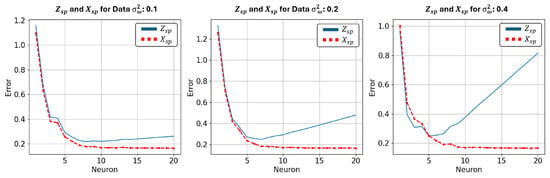
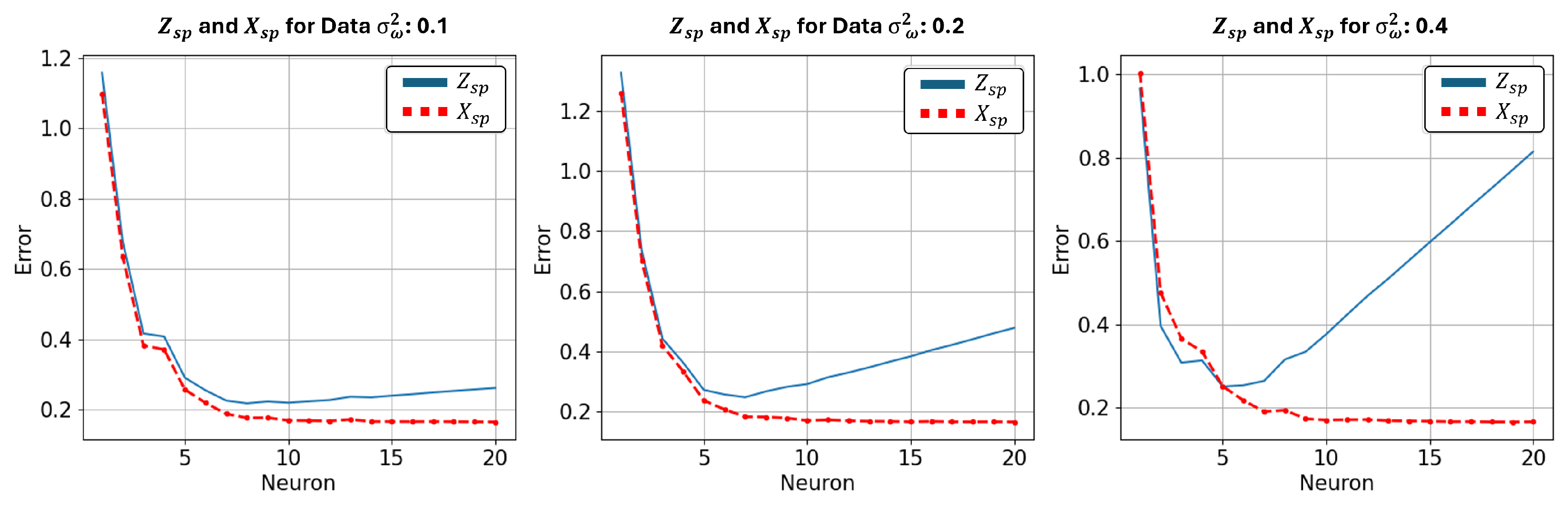
Figure 4 illustrates two key error metrics for Case 2 as noise variance increases: the available data error, $X_{s_p}$, and the unavailable reconstruction error (RE), $Z_{s_p}$. As the figure confirms, the conventional error $X_{s_p}$ measures the discrepancy between the noisy observed data and the model’s predictions and is a monotonically decreasing function of the number of neurons. In contrast, the reconstruction error $Z_{s_p}$ accounts for noise modeling and serves as a well-suited criterion for hyperparameter selection, which in this case corresponds to the number of neurons. Therefore, while using the proposed RE can provide an optimal value of the number of neurons that is close to the true number of neurons, which is five, the conventionally used MSE, in the form of data error, points to larger and larger numbers of neurons for the purpose of hyperparameter selection.

Figure 4. Behavior of the available, and conventionally used, data error ($X_{s_p}$ in (9)) and the proposed reconstruction error ($Z_{s_p}$ in (14)) for Case 2 under three different noise variances ${\sigma }_w^2=0.1,0.2$ and $0.4$. The figure shows these errors as a function of the number of neurons for when the data from Case 2 is modeled with a single-layer NN.

4.1. Impact of Additive Noise Variance in Hyperparameter Selection

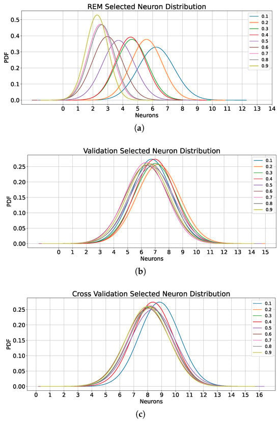
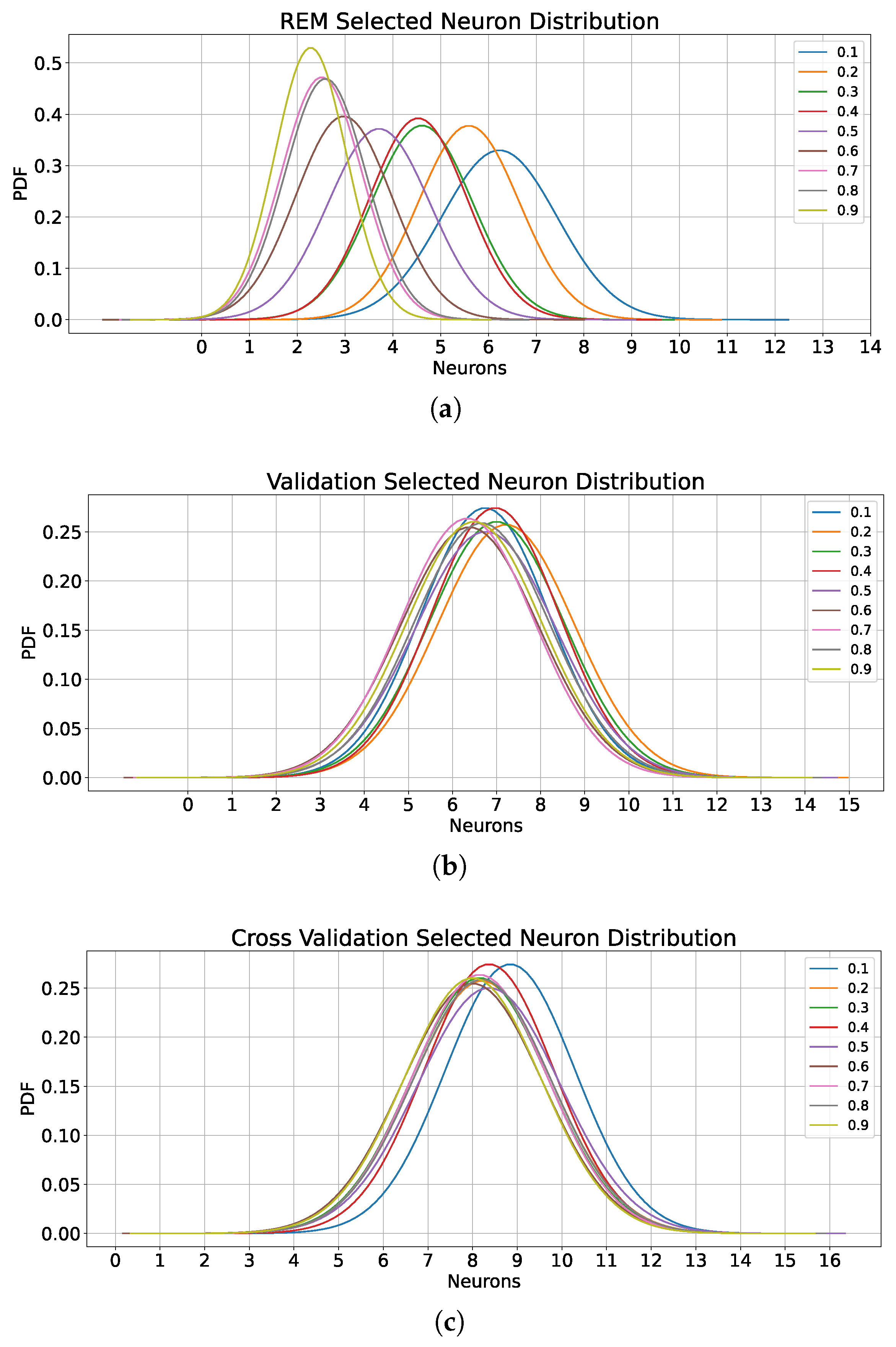
In the experiments described in this section, the data length is fixed at $n=500$. Table 2 presents the number of neurons selected for Case 1 across various noise variances in single-layer neural network modeling. As shown in the table, REM-HPS selects a much smaller number of neurons to model the data compared to the validation and cross-validation methods. Figure 5 shows the probability distributions for the number of neurons selected by the REM-HPS, validation, and cross-validation methods. As the figure illustrates, the average values reported in the table correspond to the means of these Gaussian distributions. Interestingly, as the noise variance increases, REM-HPS selects fewer neurons, reflecting its response to the effects of the additive noise variance and its power in recognizing the role of additive noise and elimination of noise modeling. In contrast, both validation approaches tend to fit more neurons on average and appear indifferent to changes in noise variance, not being able to recognize the role of the noise variance in finding the optimal number of neurons.

Table 2. Case 1 (Sine Wave): Average selected number of neurons for a one-layer architecture for a range of additive noise variances.

${\sigma }_{\omega }^2$	0.1	0.2	0.3	0.4	0.5	0.6	0.7	0.8	0.9
SNR	7.1	4.1	2.3	1.0	0.1	−0.7	−1.4	−2.0	−2.5
REM-HPS	6.5	5.1	4.5	3.4	3.0	2.9	2.7	2.5	2.2
Validation	6.7	7.2	7.1	6.8	6.4	6.3	6.7	6.5	6.4
Cross-Validation	8.8	8.2	8.2	8.4	8.4	8.3	8.2	8.2	8.3

Figure 5. Case 1: Probability Distribution Function (PDF) of selected number of neurons as a function of noise variance for one-layer modeling: (a) REM-HPS, (b) validation, (c) cross-validation.

Not only does the proposed method choose a smaller number of neurons, but the chosen NN structure also provides the smallest estimation error among the competing methods. Table 3 reports the minimum Reconstruction Mean Squared Error (R-MSE), and Table 4 reports the minimum Data Mean Squared Error (D-MSE), with both metrics evaluated on the holdout test data. As these tables illustrate, the proper choice of the number of neurons in REM-HPS in Table 2 results in lower R-MSE and D-MSE compared to the validation methods, despite the fact that REM-HPS selects fewer neurons. Note that because REM-HPS specifically targets minimization of the reconstruction error, it produces significantly lower values for this metric compared to the validation methods. Interestingly, REM-HPS also achieves lower data error MSE values, although the validation approaches are explicitly designed to minimize this error. These observations and facts confirm the superiority of REM-HPS over the validation approaches in both reconstruction error and data error minimization.

Table 3. Case 1 (Sine Wave): Average Reconstruction Mean Squared Error (R-MSE) ($Z_{S_p}$ in (14)) result of the single-layer neuron selection shown in Table 2. Bold denotes the minimum value.

${\mathit{\sigma }}_{\mathit{\omega }}^2$	0.1	0.2	0.3	0.4	0.5	0.6	0.7	0.8	0.9
REM-HPS	$\mathbf{0}.\mathbf{002}$	$\mathbf{0}.\mathbf{004}$	$\mathbf{0}.\mathbf{005}$	$\mathbf{0}.\mathbf{005}$	$\mathbf{0}.\mathbf{009}$	$\mathbf{0}.\mathbf{011}$	$\mathbf{0}.\mathbf{013}$	$\mathbf{0}.\mathbf{014}$	$\mathbf{0}.\mathbf{015}$
Validation	0.034	0.048	0.051	0.057	0.093	0.106	0.121	0.135	0.177
Cross-Validation	0.010	0.011	0.009	0.008	0.015	0.019	0.022	0.025	0.027

Table 4. Case 1 (Sine Wave): Average Data Mean Squared Error (D-MSE) ($X_{S_p}$ in (9)) result of the single-layer neuron selection shown in Table 2.

${\mathit{\sigma }}_{\mathit{\omega }}^2$	0.1	0.2	0.3	0.4	0.5	0.6	0.7	0.8	0.9
REM-HPS	$\mathbf{0}.\mathbf{011}$	$\mathbf{0}.\mathbf{042}$	$\mathbf{0}.\mathbf{091}$	$\mathbf{0}.\mathbf{160}$	$\mathbf{0}.\mathbf{248}$	$\mathbf{0}.\mathbf{361}$	$\mathbf{0}.\mathbf{475}$	$\mathbf{0}.\mathbf{628}$	$\mathbf{0}.\mathbf{786}$
Validation	0.013	0.047	0.094	0.162	0.258	0.369	0.492	0.653	0.827
Cross-Validation	0.012	0.046	0.093	0.161	0.253	0.367	0.485	0.643	0.795

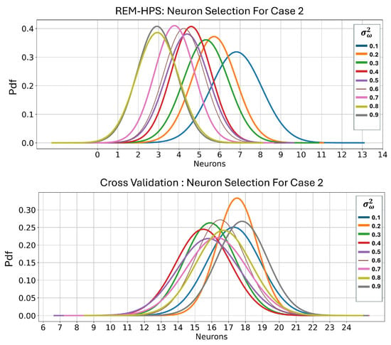
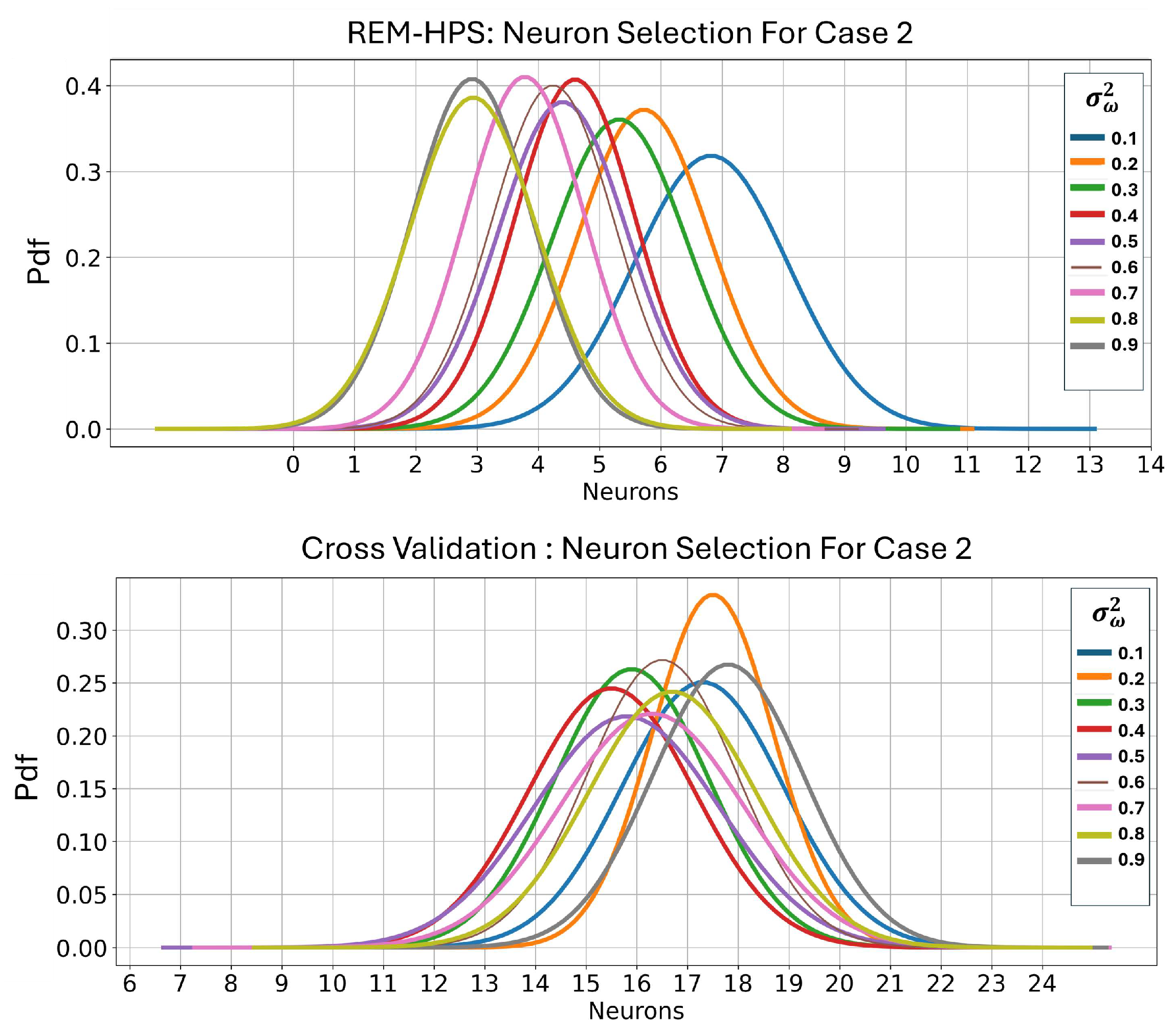
Figure 6 illustrates the results for Case 2, showing the distribution of the selected number of neurons for this single-layer neural network (NN), where the true number of neurons is five. It should be noted that the behavior of the validation method, not shown in this figure, is similar to that observed in Case 1. The corresponding average number of neurons selected by each method is reported in Table 5. In this case, where the true number of neurons is five, the proposed approach demonstrates a closer alignment with the true value compared to the validation methods. As both the table and figure show, the existing approaches choose a larger number of neurons than what is needed, which is expected to fit more of the additive noise in the NN structure. Notably, within the noise variance range of 0.15 to 0.25, the REM approach appears to have an optimal amount of data to accurately estimate the true number of neurons. However, once the data become cleaner, the modeling can accommodate more neurons. This highlights the practical role of controlled noise, or dithering, in enhancing generalization in real-world applications. Consistently, the same behavior has been observed for Case 3 for the choice of number of neurons per layer, where the number of layers is fixed at three. It is worth mentioning that the behavior of the MSEs, Reconstruction MSE and Data MSE, for Case 2 and Case 3 are similar to what is shown for Case 1 in Table 3 and Table 4. REM-HPS consistently achieves the lowest error values while selecting fewer neurons, underscoring the efficiency and effectiveness of the proposed method in avoiding noise fitting in structural modeling.

Figure 6. Case 2 (single layer with 5 neurons): Distribution of number of neurons selected by REM-HPS and cross-validation in single-layer modeling for a range of additive noise variances (means are provided in Table 5).

Table 5. Case 2 (NN—with single layer of 5 neurons): Average selected number of neurons in single-layer modeling for a range of additive noise variances.

${\mathit{\sigma }}_{\mathit{\omega }}^2$	0.1	0.2	0.3	0.4	0.5	0.6	0.7	0.8	0.9
REM-HPS	6.0	4.9	4.8	4.5	2.9	2.2	2.4	2.2	2.2
Validation	8.26	8.52	8.28	8.58	8.62	8.48	8.54	8.44	8.36
Cross-validation	17.3	17.5	15.9	15.5	15.8	16.5	16.3	17.8	15.2

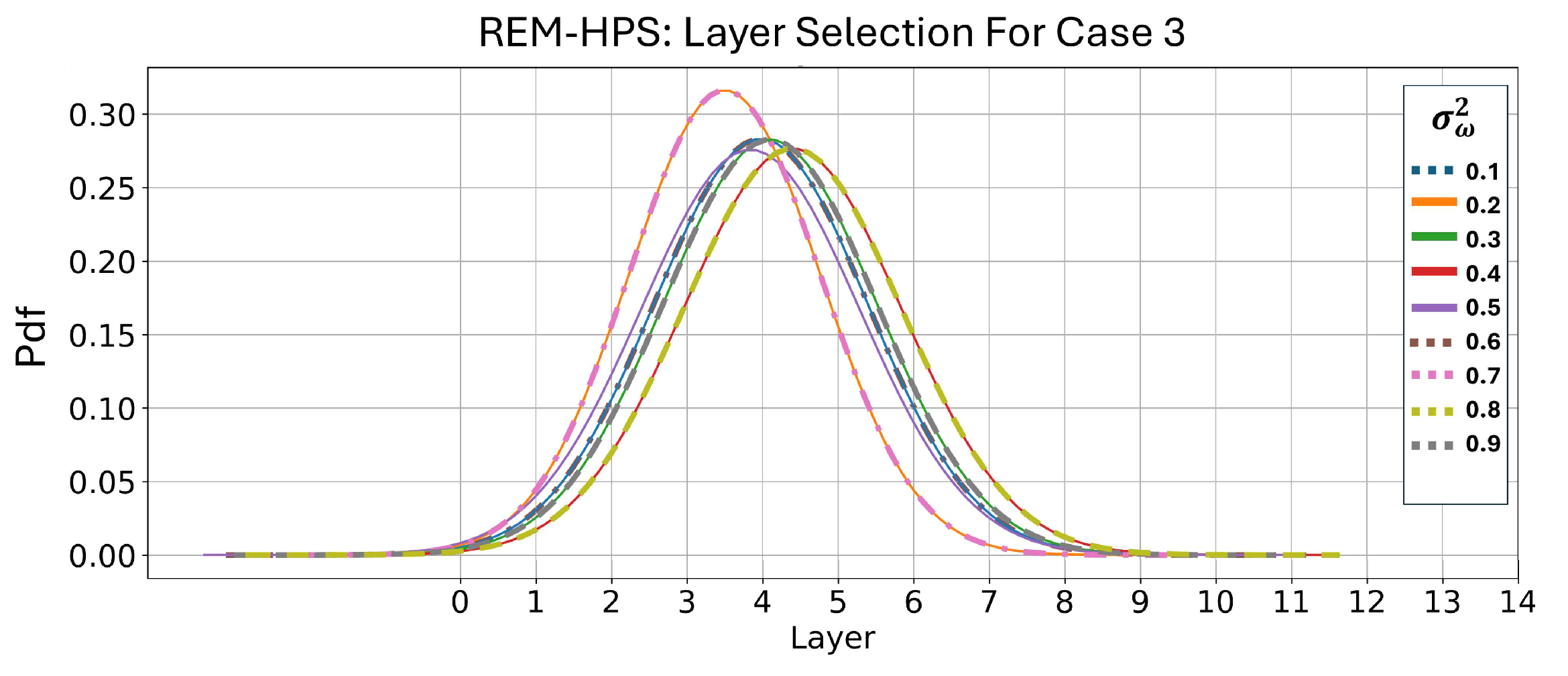
Table 6 and Figure 7 examine the role of hyperparameter selection approaches in determining the number of layers for Case 3. In this example, each layer contains five neurons. However, the results can be generalized to the simultaneous estimation of both the number of layers and neurons, where a similar performance is observed. As shown in the figure and table, the number of layers estimated by REM-HPS is close to the true value of 3, while the number estimated by validation approaches is larger and associated with higher MSE and RE. Interestingly, the results indicate that the hyperparameter selection method demonstrates greater robustness in estimating the number of layers across varying noise levels compared to its performance in selecting the number of neurons.

Table 6. Case 3 (NN with 5 Layers): Average selected number of layers in data modeling.

${\mathit{\sigma }}_{\mathit{\omega }}^2$	0.1	0.2	0.3	0.4	0.5	0.6	0.7	0.8	0.9
REM-HPS	3.9	3.5	4.1	4.4	3.8	3.9	3.5	4.1	4.4
Validation	8.6	8.2	7.3	12.3	10.9	11.7	11.0	12.2	12.3
Cross-validation	6.4	6.5	5.9	9.9	8.8	7.5	7.8	7.8	8.2

Figure 7. Case 3: Probability Density Function of REM-HPS layer number estimation as a function of noise variance (the mean is provided in Table 6).

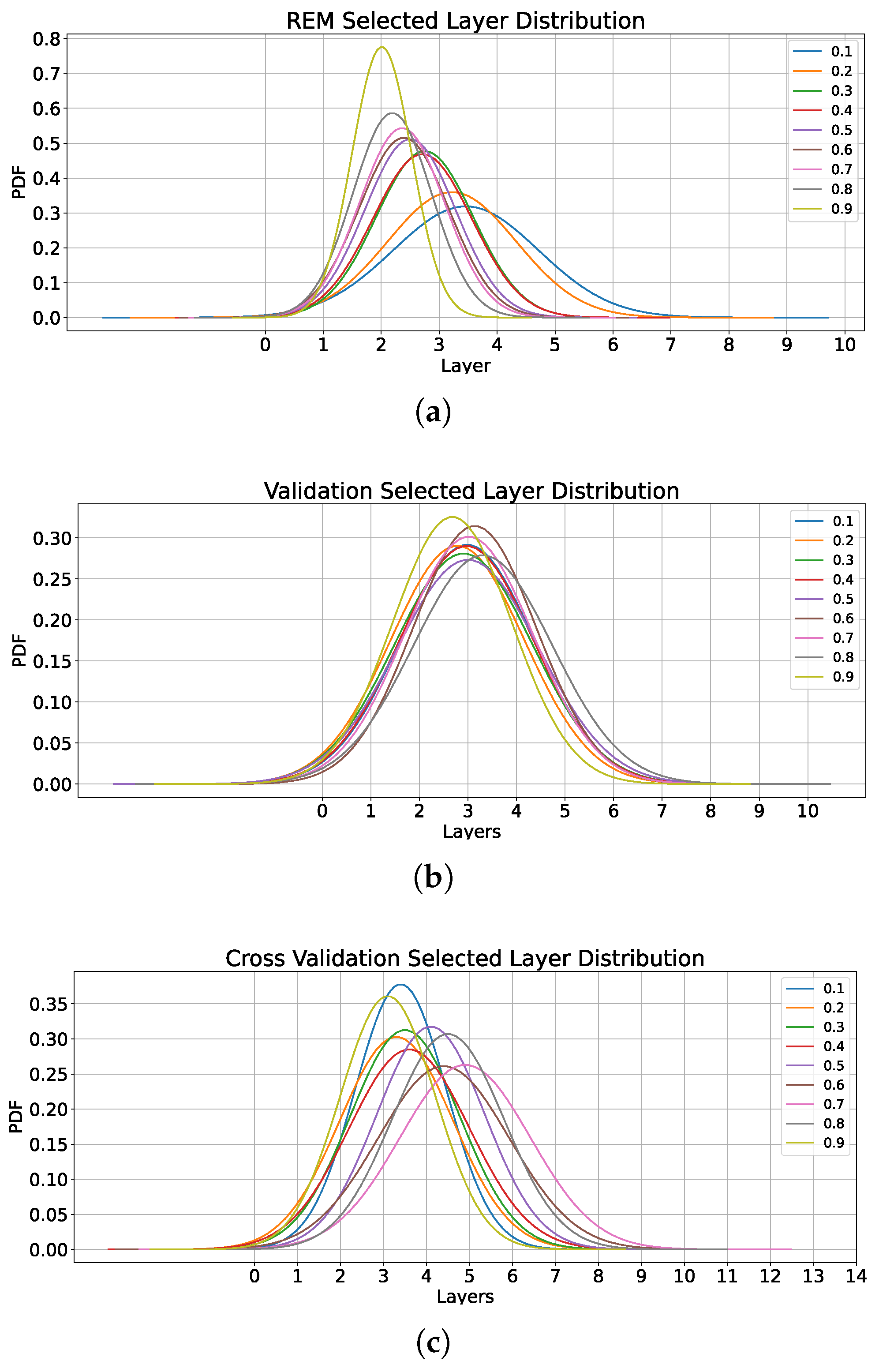
Figure 8 presents the results for Case 1, where the number of neurons per layer was fixed to five. The figure compares the number of layers selected by REM-HPS with those selected by standard validation and cross-validation methods. Compared to Figure 5, this scenario also shows that the proposed method selects smaller hyperparameter values and exhibits a behavior that manifests the role of additive noise variance. In contrast, validation approaches tend to select larger values and remain largely unaware of changes in noise. However, in this case, the cross-validation method shows a slight increase based on the noise variance. Table 7 shows the average number of selected layers, while Table 8 presents the Reconstruction MSE for this scenario. As shown in the table, the proposed method achieves a significantly lower reconstruction error while using fewer layers, highlighting its advantages over the validation methods in efficient modeling and simultaneous denoising.

Figure 8. Case 1: Distribution of selected number of layers (for 5 neurons per layer). (a) REM-HPS, (b) validation, (c) cross-validation.

Table 7. Case 1 (Sine Wave): Average selected number of layers (5 neurons per layer) for a range of additive noise variance.

${\mathit{\sigma }}_{\mathit{\omega }}^2$	0.1	0.2	0.3	0.4	0.5	0.6	0.7	0.8	0.9
REM-HPS	3.5	3.2	2.8	2.7	2.5	2.4	2.4	2.1	2.0
Validation	2.9	2.8	2.9	2.9	3.0	3.1	3.0	3.3	2.7
Cross-Validation	3.4	3.3	3.5	3.6	4.1	4.4	4.9	4.5	3.1

Table 8. Case 1 (Sine Wave): Average Reconstruction Mean Squared Error (R-MSE) ($Z_{S_p}$ in (14)) result of number-of-layer selection shown in Table 7. Bold denotes the minimum value.

${\mathit{\sigma }}_{\mathit{\omega }}^2$	0.1	0.2	0.3	0.4	0.5	0.6	0.7	0.8	0.9
REM-HPS	$\mathbf{0}.\mathbf{012}$	$\mathbf{0}.\mathbf{013}$	$\mathbf{0}.\mathbf{018}$	$\mathbf{0}.\mathbf{019}$	$\mathbf{0}.\mathbf{031}$	$\mathbf{0}.\mathbf{033}$	$\mathbf{0}.\mathbf{037}$	$\mathbf{0}.\mathbf{050}$	$\mathbf{0}.\mathbf{077}$
Validation	0.137	0.198	0.202	0.294	0.392	0.486	0.611	0.816	0.914
Cross-Validation	0.125	0.192	0.169	0.288	0.390	0.441	0.521	0.774	0.819

Table 9 shows the runtimes for when ${\sigma }_{\omega }^2$ is 0.1. The runtimes were generated using Google Colab. As expected, the validation approach has the shortest runtime, at the cost of having the highest MSE, while, also as expected, REM has a shorter runtime than the k-fold validation.

Table 9. Runtime for hyperparameter selection (HPS). One HPS run denotes a full sweep over $\mathcal{P}$. Values are mean ± std over 100 trials.

Method	Trainings	Time per HPS	Relative Time
Method	per Candidate	Run (m)	(REM = 1)
REM-HPS	1	34.6 ± 2.9	1.00
Validation	1	27.8 ± 2.5	0.80
k-fold CV ($k=5$)	5	138.9 ± 11.6	4.01

4.2. Impact of Data Length in Hyperparameter Section

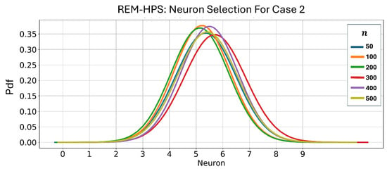
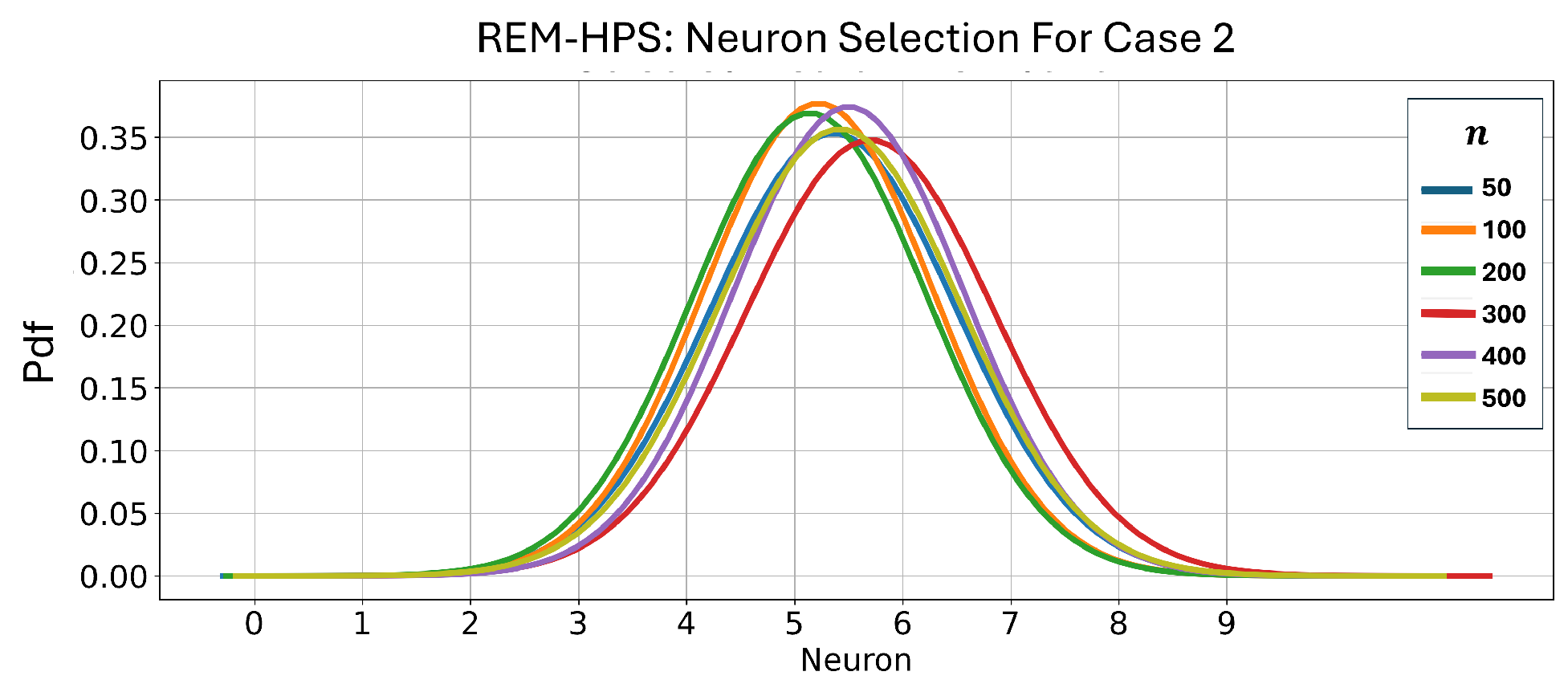
Figure 9 and Table 10 illustrate how the estimated number of neurons varies with data length for Case 2 when the additive noise variance is ${\sigma }_w^2=0.2$. As shown in the table, REM-HPS selects a smaller number of neurons. Moreover, the selected value not only is smaller but also matches the true number of neurons. Note that a similar behavior is observed for Case 1 and Case 2 as the data length increases. A similar result was observed for Case 3, where the proposed method selects the correct number of neurons and layers. In contrast, validation approaches select larger models, and the size of these models continued to grow with the data length. It is worth mentioning that, similarly to previous experiments, the proposed approach yields the minimum Reconstruction and Data MSE values, confirming again the superiority of the proposed method in simultaneous hyperparameter selection and denoising.

Figure 9. Case 2: Probability Density Function (Pdf) of selected neurons as a function of data length (means are provided in Table 10.

Table 10. Case 2 (NN with single layer and five neurons): Average selected number of neurons as a function of data length for a range of data lengths (additive noise variance is ${\sigma }_w^2=0.2$).

Data Length (n)	50	100	200	300	400	500
REM-HPS	5.3	5.2	5.1	5.7	5.5	5.4
Validation	10.3	10.8	10.8	10.9	11.3	11.0
Cross-Validation	14.3	14.3	15.2	15.8	16.1	16.0

4.3. Practical Role of the Universal Approximation Theorem in REM-HPS

The Universal Approximation Theorem (UAT) declares that for any given continuous function, the neural network with a certain structure is capable of approximating the function to any desired degree of accuracy [49]. It is important to emphasize that these results are existence theorems. They ensure that a network with an appropriate structure exists, but they do not explain how to determine the network’s parameters (i.e., how to train it), nor do they precisely characterize how large the network must be to represent a particular function. Identifying a suitable network in practice therefore remains a challenging task, typically approached using conventional optimization methods such as backpropagation, which is used in this work.

In this work, the reference to the UAT serves a practical and empirical purpose, rather than a theoretical one. Specifically, let us model the deep five-layer network in Case 3 with a single hidden layer with a free number of neurons. According to the UAT applied to the feedforward network, this structure acts as a universal approximator. However, when the number of neurons increases beyond what is needed to approximate the underlying function, the model begins to fit the additive output noise that appears in (6). This effect is clearly reflected in the conventional use of the available data error $X_{S_p}$ defined in (9), which decreases monotonically with model complexity, regardless of whether additional neurons improve generalization performance.

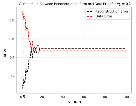
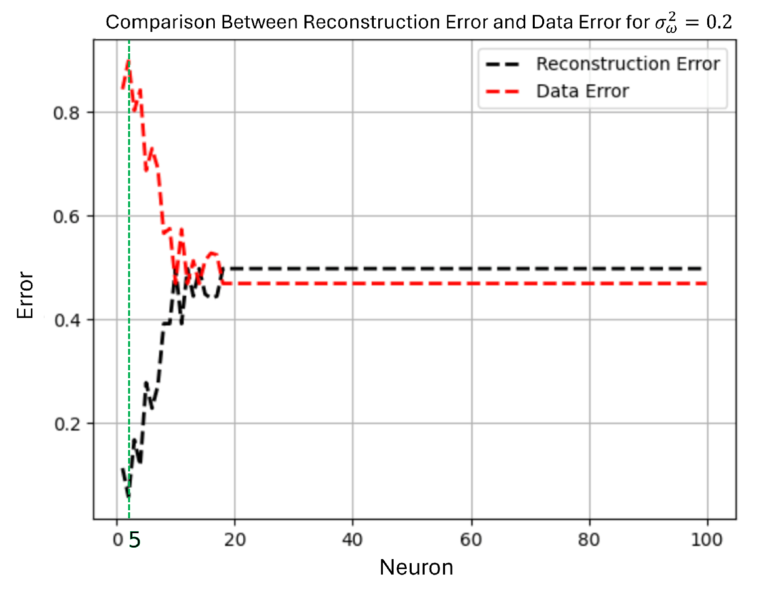
Figure 10 illustrates this phenomenon: when single-layer networks with increasing width are trained to approximate the deep target of Case 3, the data error continues to decrease for larger networks. This decreasing trend misleadingly suggests improved performance, even though the additional neurons in fact capture noise rather than a meaningful structure. By contrast, the reconstruction error $Z_{S_p}$ defined in (14) and estimated using REM-HPS provides an accurate indicator of overfitting. Once the model begins fitting noise, the reconstruction error increases, signaling that the network has exceeded the effective model order required for the task.

Figure 10. Comparison of the available, and conventionally used, Data MSE $X_{S_p}$ in (9) and the proposed Reconstruction MSE $Z_{S_p}$ in (14) as the number of neurons increases in a single-layer estimation of Case 3. While the Data MSE decreases monotonically with model width, falsely suggesting improved performance, the Reconstruction MSE correctly identifies the onset of noise overfitting, choosing 5 neurons (shown in green dash line), demonstrating the practical advantage of REM-HPS for structural hyperparameter selection.

This behavior highlights a key advantage of REM-HPS: by focusing on minimizing an estimate of the Reconstruction MSE, the proposed method penalizes noise-fitting architectures, even when the Data MSE favors larger models. Consequently, REM-HPS consistently selects the smallest architecture capable of approximating the target function, achieving the approximation capability implied by the UAT without absorbing noise into the predicted output. In the example of Figure 10, REM-HPS selects a compact single-layer model that achieves Reconstruction and Data MSE values comparable to those achieved by the true deep architecture, while validation-based methods continue to expand the network unnecessarily. The proposed REM-HPS framework does not depend on the UAT for its derivation or theoretical validity. However, the UAT provides a conceptual backdrop to interpret the empirical advantages of reconstruction-based hyperparameter selection in avoiding overfitting in the presence of additive noise.

4.4. Real-World Dataset Validation

To validate the effectiveness of REM-HPS on practical applications, we conducted extensive experiments on two real-world engineering datasets: the Energy Efficiency dataset and the Concrete Compressive Strength dataset. These experiments assess the proposed method in practical applications in actual regression tasks.

• Energy Efficiency Dataset: This dataset contains 768 samples with eight features representing building parameters (relative compactness, surface area, wall area, roof area, overall height, orientation, glazing area, and glazing area distribution). The target variable is the heating load required for the building, measured in kWh/m².
• Concrete Compressive Strength Dataset: This dataset comprises 1030 samples with eight features describing concrete mixture components (cement, blast furnace slag, fly ash, water, superplasticizer, coarse aggregate, fine aggregate, and age). The target variable is the compressive strength, measured in MPa.

For both datasets, Gaussian noise with varying SNRs was artificially added to the target output to simulate real-world measurement uncertainties. The experiments were conducted across multiple SNR levels (20, 15, 10, 5, and 0 dB) and different training set sizes (200, 400, and 600 samples) to evaluate robustness. We tested neural network architectures with 1 to 3 hidden layers and 5 to 20 neurons per layer. Each configuration was evaluated over 100 independent trials, and five-fold cross-validation was employed for the validation-based approaches. All models were trained using the Adam optimizer with a learning rate of 0.01 for 300 epochs.

Table 11 presents the average Reconstruction MSE across different SNR levels for both datasets. As demonstrated in the table, REM-HPS consistently achieves lower reconstruction error compared to cross-validation, with more improvement for the Energy Efficiency dataset (averaging 9.18% improvement) compared to the Concrete dataset (averaging 0.89% improvement). This difference can be attributed to the distinct characteristics of the datasets. The Energy Efficiency dataset exhibits stronger nonlinear relationships between features and the target, making it more susceptible to overfitting when using validation-based methods that tend to select overly complex architectures.

Table 11. Real-world datasets: Average Reconstruction MSE across SNR levels.

Dataset	Method	SNR = 20 dB	SNR = 15 dB	SNR = 10 dB	SNR = 5 dB	SNR = 0 dB
Energy Efficiency	REM-HPS	0.062	0.071	0.082	0.095	0.112
	Cross-Validation	0.068	0.079	0.093	0.108	0.125
Concrete Strength	REM-HPS	0.178	0.186	0.197	0.211	0.228
	Cross-Validation	0.180	0.189	0.201	0.215	0.232

Notably, REM-HPS demonstrates superior noise-dependent modeling, adapting its architectural selections based on the noise level. As the SNR decreases (noise increases), REM-HPS selects progressively simpler architectures, thereby avoiding the pitfall of fitting noise components. In contrast, cross-validation exhibits limited differentiation to the noise variance, often selecting unnecessarily complex models regardless of the noise level. This behavior is consistent with our observations in the synthetic data experiments presented in Section 4. Table 12 shows the runtime as a function of training size, which is consistent with the computational complexity provided in Section 3.2.

Table 12. Runtime vs. training set size for real-world experiments. Each entry is mean ± std minutes per HPS run (full sweep over $\mathcal{P}$).

Method	$\mathit{n}=200$	$\mathit{n}=400$	$\mathit{n}=600$
REM-HPS	12.4 ± 1.1	23.0 ± 1.8	33.7 ± 2.6
5-fold CV	49.6 ± 4.2	93.1 ± 7.6	137.5 ± 10.9

Table 13 illustrates the impact of training set size on Reconstruction MSE for a fixed noise variance (corresponding to SNR ≈ 10 dB). The results demonstrate that REM-HPS maintains consistent performance across varying data lengths, efficiently utilizing available samples without requiring data splitting. On the other hand, cross-validation performance shows greater variability with data length, as the subdivision of data into training and validation folds becomes more critical with smaller datasets. For the Energy Efficiency dataset with only 200 training samples, REM-HPS achieves 0.089 Reconstruction MSE compared to 0.101 for cross-validation, representing 11.9% improvement. This advantage becomes less significant but persists as data length increases, confirming that REM-HPS is particularly beneficial in scenarios where the data is limited.

Table 13. Real-world datasets: Average Reconstruction MSE as a function of training set size (${\sigma }_{\omega }^2=0.3$, SNR ≈ 10 dB).

Dataset	Method	$\mathit{n}=200$	$\mathit{n}=400$	$\mathit{n}=600$	Overall
Energy Efficiency	REM-HPS	0.089	0.081	0.078	0.085
	Cross-Validation	0.101	0.091	0.086	0.093
Concrete Strength	REM-HPS	0.206	0.197	0.192	0.202
	Cross-Validation	0.209	0.201	0.196	0.204

5. Conclusions

This paper successfully addressed the persistent challenges of structural hyperparameter selection (HPS) in neural network (NN) regression, specifically the limitations imposed by output noise and the required validation-based data partitioning. We proposed the Reconstruction Error Minimization for Hyperparameter Selection (REM-HPS) framework, grounded in statistical learning theory, which offers a practical and theoretically sound solution for architectural optimization. The core innovation of REM-HPS lies in redefining the selection objective: instead of minimizing the conventional Data MSE, which is heavily influenced by noise, we reliably estimate and minimize the Reconstruction MSE, which reflects the model’s true, noise-independent ability to reconstruct the underlying function. The proposed methodology delivers three major contributions essential for high-quality machine learning model design: 1—Deterministic and Efficient Selection: REM-HPS enables the deterministic selection of the optimal NN architecture without requiring data splitting or cross-validation. This use of the entire dataset for training significantly improves sample efficiency and reduces the computational complexity associated with iterative partitioning schemes. 2—Superior Generalization and Parsimony: By explicitly accounting for the Signal-to-Noise Ratio (SNR), the criterion inherently penalizes excessive complexity, selecting the most parsimonious model structure. Our empirical analysis confirms that REM-HPS consistently achieves superior estimation accuracy and significantly mitigates overfitting compared to traditional validation approaches. 3—Principled Structural Selection Consistent with Universality: The method provides an effective approach to structural HPS that efficiently considers the role of output noise, thereby guiding the NN towards a minimal architecture that practically manifests the capabilities guaranteed by the universal approximation theorem.

The deterministic and noise-aware nature of the REM-HPS criterion provides a robust foundation for automated, resource-efficient HPS in the broader field of statistical learning. The superiority and efficiency of REM-HPS over validation approaches were rigorously demonstrated in three tactically designed experimental setups, as well as two real-world datasets. Although this work presented the behavior of REM-HPS in selecting structural hyperparameters, such as the number of layers and neurons per layer in shallow NN modeling, the proposed method can be generalized to choose the optimal activation function, as well as to select training hyperparameters, such as batch number, epoch number, and learning. Future work will also focus on extending the REM-HPS criterion to optimize non-structural hyperparameters, such as regularization coefficients, and applying the framework to a wider class of nonlinear systems.

References

- Tipping, M.E.; Bishop, C.M. Probabilistic principal component analysis. J. R. Stat. Soc. Ser. B Stat. Methodol. 1999, 61, 611–622. [Google Scholar] [CrossRef] [Scilit]
- Blundell, C.; Cornebise, J.; Kavukcuoglu, K.; Wierstra, D. Weight uncertainty in neural network. In Proceedings of the International Conference on Machine Learning; PMLR: New York, NY, USA, 2015; pp. 1613–1622. [Google Scholar]
- Victoria, A.H.; Maragatham, G. Automatic tuning of hyperparameters using Bayesian optimization. Evol. Syst. 2021, 12, 217–223. [Google Scholar] [CrossRef] [Scilit]
- Stuke, A.; Rinke, P.; Todorović, M. Efficient hyperparameter tuning for kernel ridge regression with Bayesian optimization. Mach. Learn. Sci. Technol. 2021, 2, 035022. [Google Scholar] [CrossRef] [Scilit]
- Yang, X.; Wang, J.; Zhao, X.; Li, S.; Tao, Z. Calibrate automated graph neural network via hyperparameter uncertainty. In Proceedings of the 31st ACM International Conference on Information & Knowledge Management; Association for Computing Machinery: New York, NY, USA, 2022; pp. 4640–4644. [Google Scholar]
- Tiep, N.H.; Jeong, H.Y.; Kim, K.D.; Xuan Mung, N.; Dao, N.N.; Tran, H.N.; Hoang, V.K.; Ngoc Anh, N.; Vu, M.T. A New Hyperparameter Tuning Framework for Regression Tasks in Deep Neural Network: Combined-Sampling Algorithm to Search the Optimized Hyperparameters. Mathematics 2024, 12, 3892. [Google Scholar] [CrossRef] [Scilit]
- Liao, L.; Li, H.; Shang, W.; Ma, L. An empirical study of the impact of hyperparameter tuning and model optimization on the performance properties of deep neural networks. ACM Trans. Softw. Eng. Methodol. (TOSEM) 2022, 31, 53. [Google Scholar] [CrossRef] [Scilit]
- Hsu, C.W.; Chang, C.C.; Lin, C.J. A Practical Guide to Support Vector Classification. 2003. Available online: https://eecs.csuohio.edu/~sschung/DSA460/SVM_guide.pdf (accessed on 1 January 2026).
- El-Shahat, D.; Tolba, A.; Abouhawwash, M.; Abdel-Basset, M. Machine learning and deep learning models based grid search cross validation for short-term solar irradiance forecasting. J. Big Data 2024, 11, 134. [Google Scholar] [CrossRef] [Scilit]
- Chen, S.R.; Chen, S.J.; Hsieh, W.B. Enhancing Machine Learning-Based DDoS Detection Through Hyperparameter Optimization. Electronics 2025, 14, 3319. [Google Scholar] [CrossRef] [Scilit]
- Bergstra, J.; Bengio, Y. Random search for hyper-parameter optimization. J. Mach. Learn. Res. 2012, 13, 281–305. [Google Scholar]
- Pedregosa, F. Hyperparameter optimization with approximate gradient. In Proceedings of the International Conference on Machine Learning; PMLR: New York, NY, USA, 2016; pp. 737–746. [Google Scholar]
- Dong, X.; Shen, J.; Wang, W.; Shao, L.; Ling, H.; Porikli, F. Dynamical hyperparameter optimization via deep reinforcement learning in tracking. IEEE Trans. Pattern Anal. Mach. Intell. 2019, 43, 1515–1529. [Google Scholar] [CrossRef] [Scilit]
- Jiang, W.; Siddiqui, S. Hyper-parameter optimization for support vector machines using stochastic gradient descent and dual coordinate descent. EURO J. Comput. Optim. 2020, 8, 85–101. [Google Scholar] [CrossRef] [Scilit]
- Wu, J.; Chen, S.; Liu, X. Efficient hyperparameter optimization through model-based reinforcement learning. Neurocomputing 2020, 409, 381–393. [Google Scholar] [CrossRef] [Scilit]
- Chen, C.H.; Lai, J.P.; Chang, Y.M.; Lai, C.J.; Pai, P.F. A Study of Optimization in Deep Neural Networks for Regression. Electronics 2023, 12, 3071. [Google Scholar] [CrossRef] [Scilit]
- Shanthi, D.; Chethan, N. Genetic algorithm based hyper-parameter tuning to improve the performance of machine learning models. SN Comput. Sci. 2022, 4, 119. [Google Scholar] [CrossRef] [Scilit]
- Catalin, A.; Andonie, R. Weighted Random Search for Hyperparameter Optimization. Int. J. Comput. Commun. Control 2019, 14, 154–169. [Google Scholar]
- Maclaurin, D.; Duvenaud, D.; Adams, R. Gradient-based hyperparameter optimization through reversible learning. In Proceedings of the International Conference on Machine Learning; PMLR: lNew York, NY, USA, 2015; pp. 2113–2122. [Google Scholar]
- Ali, A.; Dobriban, E.; Tibshirani, R. The implicit regularization of stochastic gradient flow for least squares. In Proceedings of the International Conference on Machine Learning; PMLR: New York, NY, USA, 2020; pp. 233–244. [Google Scholar]
- Feurer, M.; Letham, B.; Hutter, F.; Bakshy, E. Practical transfer learning for bayesian optimization. arXiv 2018, arXiv:1802.02219. [Google Scholar]
- Barbu, A. Training a two-layer ReLU network analytically. Sensors 2023, 23, 4072. [Google Scholar] [CrossRef] [Scilit]
- Shin, C.Y.; Choi, Y.S.; Kim, M.S. Data Augmentation-Based Enhancement for Efficient Network Traffic Classification. IEEE Access 2025, 13, 6006–6028. [Google Scholar] [CrossRef] [Scilit]
- Drobnič, F.; Starc, G.; Jurak, G.; Kos, A.; Pustišek, M. Explained Learning and Hyperparameter Optimization of Ensemble Estimator on the Bio-Psycho-Social Features of Children and Adolescents. Electronics 2023, 12, 4097. [Google Scholar] [CrossRef] [Scilit]
- Borboudakis, G.; Tsamardinos, I. Forward-Backward Selection with Early Dropping. J. Mach. Learn. Res. 2019, 20, 1–39. [Google Scholar]
- Tsamardinos, I.; Borboudakis, G.; Katsogridakis, P.; Pratikakis, P.; Christophides, V. A greedy feature selection algorithm for big data of high dimensionality. Mach. Learn. 2019, 108, 149–202. [Google Scholar] [CrossRef] [Scilit] [PubMed]
- Hutter, F.; Hoos, H.H.; Leyton-Brown, K. Identifying key algorithm parameters and instance features using forward selection. In Proceedings of the International Conference on Learning and Intelligent Optimization; Springer: Berlin/Heidelberg, Germany, 2013; pp. 364–381. [Google Scholar]
- Fiedler, L.; Hoffmann, N.; Mohammed, P.; Popoola, G.A.; Yovell, T.; Oles, V.; Ellis, J.A.; Rajamanickam, S.; Cangi, A. Training-free hyperparameter optimization of neural networks for electronic structures in matter. Mach. Learn. Sci. Technol. 2022, 3, 045008. [Google Scholar] [CrossRef] [Scilit]
- Cruz-Martinez, J.; Jansen, A.; van Oord, G.; Rabemananjara, T.R.; Rocha, C.M.; Rojo, J.; Stegeman, R. Hyperparameter optimisation in deep learning from ensemble methods: Applications to proton structure. Mach. Learn. Sci. Technol. 2025, 6, 025027. [Google Scholar] [CrossRef] [Scilit]
- Braga-Neto, U.M.; Dougherty, E.R. Is cross-validation valid for small-sample microarray classification? Bioinformatics 2004, 20, 374–380. [Google Scholar] [CrossRef] [Scilit]
- Soper, D.S. Greed Is Good: Rapid Hyperparameter Optimization and Model Selection Using Greedy k-Fold Cross Validation. Electronics 2021, 10, 1973. [Google Scholar] [CrossRef] [Scilit]
- Meyer, R.; Musco, C. The Statistical Cost of Robust Kernel Hyperparameter Tuning. Adv. Neural Inf. Process. Syst. 2020, 33, 21334–21345. [Google Scholar]
- Antorán, J.; Allingham, J.; Hernández-Lobato, J.M. Depth uncertainty in neural networks. Adv. Neural Inf. Process. Syst. 2020, 33, 10620–10634. [Google Scholar]
- Hutter, F.; Hoos, H.H.; Leyton-Brown, K. Sequential model-based optimization for general algorithm configuration. In Proceedings of the Learning and Intelligent Optimization: 5th International Conference, LION 5, Rome, Italy, 17–21 January 2011; Selected Papers 5; Springer: Berlin/Heidelberg, Germany, 2011; pp. 507–523. [Google Scholar]
- Qi, J.; Du, J.; Siniscalchi, S.M.; Ma, X.; Lee, C.H. On Mean Absolute Error for Deep Neural Network Based Vector-to-Vector Regression. IEEE Signal Process. Lett. 2020, 27, 1485–1489. [Google Scholar] [CrossRef] [Scilit]
- Lederer, J. Risk Bounds for Robust Deep Learning. arXiv 2020, arXiv:2009.06202. [Google Scholar] [CrossRef] [Scilit]
- Terven, J.; Cordova-Esparza, D.M.; Romero-González, J.A.; Ramírez-Pedraza, A.; Chávez-Urbiola, E. A comprehensive survey of loss functions and metrics in deep learning. Artif. Intell. Rev. 2025, 58, 195. [Google Scholar] [CrossRef] [Scilit]
- Ciampiconi, L.; Elwood, A.; Leonardi, M.; Mohamed, A.; Rozza, A. A survey and taxonomy of loss functions in machine learning. arXiv 2023, arXiv:2301.05579. [Google Scholar] [CrossRef] [Scilit]
- Bishop, C.M. Pattern Recognition and Machine Learning; Springer: Berlin/Heidelberg, Germany, 2006. [Google Scholar]
- Dong, G.; Basu, A. Medical image denoising via explainable ai feature preserving loss. In Proceedings of the International Conference on Smart Multimedia; Springer: Berlin/Heidelberg, Germany, 2024; pp. 17–32. [Google Scholar]
- Beheshti, S.; Shamsi, M. ϵ-Confidence Approximately Correct (ϵ-CoAC) Learnability and Hyperparameter Selection in Linear Regression Modeling. IEEE Access 2025, 13, 14273–14289. [Google Scholar] [CrossRef] [Scilit]
- Shamsi, M.; Beheshti, S. Relative Entropy (RE)-Based LTI System Modeling Equipped With Simultaneous Time Delay Estimation and Online Modeling. IEEE Access 2023, 11, 113885–113899. [Google Scholar] [CrossRef] [Scilit]
- Beheshti, S.; Sedghizadeh, S. Number of Source Signal Estimation by the Mean Squared Eigenvalue Error. IEEE Trans. Signal Process. 2018, 66, 5694–5704. [Google Scholar] [CrossRef] [Scilit]
- Beheshti, S.; Naghsh, E.; Sadat-Nejad, Y.; Naderahmadian, Y. Multimodal Mutual Information Extraction and Source Detection with Application in Focal Seizure Localization. Electronics 2025, 14, 4897. [Google Scholar] [CrossRef] [Scilit]
- Beheshti, S.; Bommanahally, V. Minimum Mismatch Modeling (3M) Hyperparameter Selection in Autoregressive Moving Average (ARMA) Modeling. IEEE Access 2025, 13, 133681–133693. [Google Scholar] [CrossRef] [Scilit]
- Beheshti, S.; Shamsi, M.; Sadat-Nejad, Y.; Zhou, M. Polynomial Regression Hyperparameter Selection and Analysis using Reconstruction Error Minimization (REM). In Proceedings of the 2024 11th IEEE Swiss Conference on Data Science (SDS); IEEE: Piscataway, NJ, USA, 2024; pp. 8–15. [Google Scholar] [CrossRef] [Scilit]
- Wu, J.; Chen, X.Y.; Zhang, H.; Xiong, L.D.; Lei, H.; Deng, S.H. Hyperparameter optimization for machine learning models based on Bayesian optimization. J. Electron. Sci. Technol. 2019, 17, 26–40. [Google Scholar]
- Hu, X.; Wen, S.; Lam, H.K. Improvement accuracy in deep learning: An increasing neurons distance approach with the penalty term of loss function. Inf. Sci. 2023, 644, 119268. [Google Scholar] [CrossRef] [Scilit]
- Kratsios, A. The universal approximation property: Characterization, construction, representation, and existence. Ann. Math. Artif. Intell. 2021, 89, 435–469. [Google Scholar] [CrossRef] [Scilit]
Disclaimer/Publisher’s Note: The statements, opinions and data contained in all publications are solely those of the individual author(s) and contributor(s) and not of MDPI and/or the editor(s). MDPI and/or the editor(s) disclaim responsibility for any injury to people or property resulting from any ideas, methods, instructions or products referred to in the content. |
© 2026 by the authors. Licensee MDPI, Basel, Switzerland. This article is an open access article distributed under the terms and conditions of the Creative Commons Attribution (CC BY) license.