EEMD-TiDE-Based Passenger Flow Prediction for Urban Rail Transit

Abstract

Urban rail transit networks in developing countries are rapidly expanding, entering a networked operational phase where accurate passenger flow forecasting is crucial for optimizing vehicle scheduling, resource allocation, and transportation efficiency. In the short term, accurate real-time forecasting enables the dynamic adjustment of train headways and crew deployment, reducing average passenger waiting times during peak hours and alleviating platform overcrowding; in the long term, reliable trend predictions support strategic planning, including capacity expansion, station retrofitting, and energy management. This paper proposes a novel hybrid forecasting model, EEMD-TiDE, that combines improved Ensemble Empirical Mode Decomposition (EEMD) with a Time Series Dense Encoder (TiDE) to enhance prediction accuracy. The EEMD algorithm effectively overcomes mode mixing issues in traditional EMD by incorporating white noise perturbations, decomposing raw passenger flow data into physically meaningful Intrinsic Mode Functions (IMFs). At the same time, the TiDE model, a linear encoder–decoder architecture, efficiently handles multi-scale features and covariates without the computational overhead of self-attention mechanisms. Experimental results using Xi’an Metro passenger flow data (2017–2019) demonstrate that EEMD-TiDE significantly outperforms baseline models. This study provides a robust solution for urban rail transit passenger flow forecasting, supporting sustainable urban development.

1. Introduction

With the continuous expansion of urban rail transit networks in developing countries, system operations have entered a networked phase. Accurate segment flow forecasting is crucial for formulating scientific vehicle scheduling schemes, optimizing emergency resource allocation, enhancing passenger transport efficiency, and reducing operational costs, thereby supporting sustainable urban development [1]. Meanwhile, a robust passenger flow prediction model accurately identifies high-demand areas and temporal fluctuation patterns, thereby establishing a scientifically rigorous foundation for optimizing resource deployment strategies [2]. Traffic prediction models can be broadly categorized into three types: parametric models, non-parametric models, and hybrid models.

Parametric models, such as ARIMA (Autoregressive Integrated Moving Average) [3] and Kalman filtering [4], are grounded on statistical assumptions, requiring time series data to assure stationarity. Non-parametric models encompass a broader range of methodologies, including k-nearest neighbors [5], artificial neural networks [6], support vector machines (SVMs) [7], and language models [8]. These approaches excel at avoiding complex parameter settings and mitigating noise interference. However, they often suffer from opaque training processes, a reliance on extensive historical data, and computationally intensive operations. Hybrid models integrate the advantages of multiple algorithms to overcome limitations of single models, thereby significantly enhancing their predictive robustness [9].

In recent years, hybrid modeling methods based on time series decomposition have attracted considerable attention [10,11,12,13]. These approaches decompose original data into multiple sub-series, fit each component with an adaptive model, and ultimately improve prediction accuracy through aggregation. Huang et al.’s Hilbert–Huang Transform (HHT) [14] represents a groundbreaking advancement in signal processing. Compared to traditional wavelet and Fourier transforms, which face limitations in handling complex signals, HHT theoretically decomposes any signal into several Intrinsic Mode Functions (IMFs) [15] that contain diverse frequency characteristics, trend terms, and residual components. Its early applications demonstrate its effectiveness for temperature forecasting [16], financial analysis [17,18], power load prediction [19], and hydrological forecasting [20]. Notably, existing hybrid models like ARIMA-LSTM primarily focus on single-sequence prediction, inadequately addressing correlations among prediction samples.

To address the efficiency limitations of Transformer-based models in time series forecasting, this study innovatively integrates the TiDE (Time Series Dense Encoder) architecture—a dense MLP framework that efficiently handles nonlinear dependencies and dynamic covariates—into a novel hybrid model (EEMD-TiDE) for urban rail transit passenger flow forecasting. The framework employs a dual-stage structure: (1) raw data undergo EEMD (which introduces white noise to resolve mode mixing in conventional EMD), yielding physically meaningful Intrinsic Mode Functions (IMFs); (2) each IMF is processed independently by TiDE for precise prediction. This integration achieves three key advancements:

(1)

Architectural synergy: TiDE’s channel-independent assumption (transforming multivariate forecasting into parallel univariate tasks) perfectly aligns with EEMD’s IMF components (each a stationary time series). Its residual block (with dropout, ReLU, residual connections, and LayerNorm) further optimizes feature extraction from decomposed signals.

(2)

Computational efficiency: EEMD’s O(N²) complexity (N = sequence length) and TiDE’s O(L·H) forecasting complexity (L = lookback window, H = horizon) enable high-accuracy predictions without processing raw non-stationary data, preserving efficiency while enhancing performance.

(3)

Hierarchical covariate utilization: TiDE’s unified treatment of static/dynamic covariates is synergized with EEMD’s multi-resolution decomposition, enabling a differential covariate–IMF association analysis for refined feature learning.

Unlike Transformers, which face efficiency and generalization challenges in time series, the EEMD-TiDE framework leverages TiDE’s linear-model-like efficiency while modeling complex covariates. By synergistically combining EEMD’s noise-robust decomposition with TiDE’s sequential modeling, this hybrid approach significantly improves forecasting accuracy and stability in capturing both short-term fluctuations and long-term trends in urban transit systems.

2. Methodology

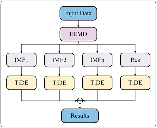
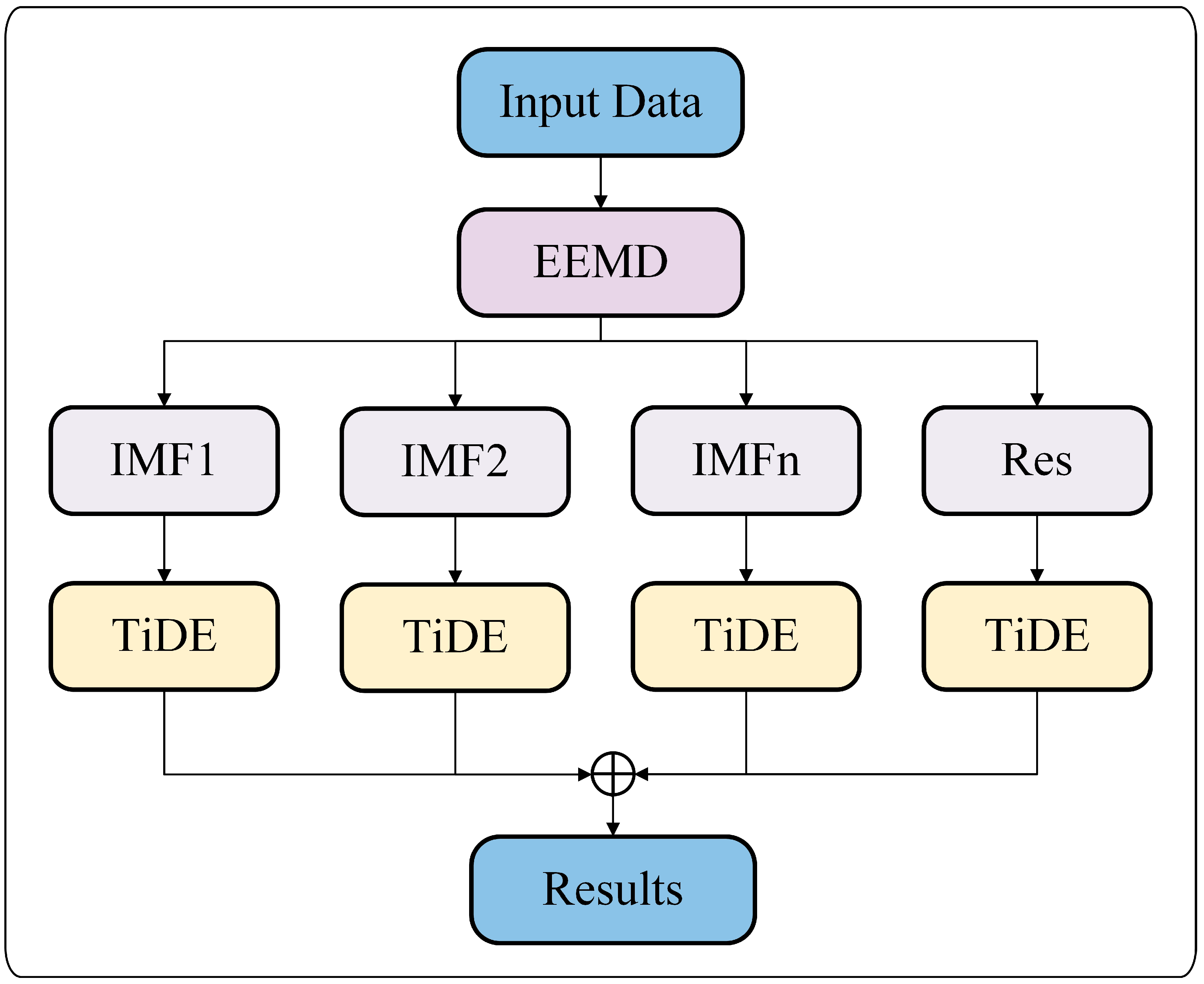
To enhance the prediction accuracy of passenger flow sequences, this paper proposes a passenger flow forecasting model called EEMD-TiDE. In this section, we first analyze the components of the model as well as the learning and application methodologies. Subsequently, the fundamental concept of the hybrid algorithm is introduced. Figure 1 illustrates the architectural framework of the EEMD-TiDE model.

Figure 1. The flowchart of EEMD-TiDE.

2.1. Decomposition: EEMD

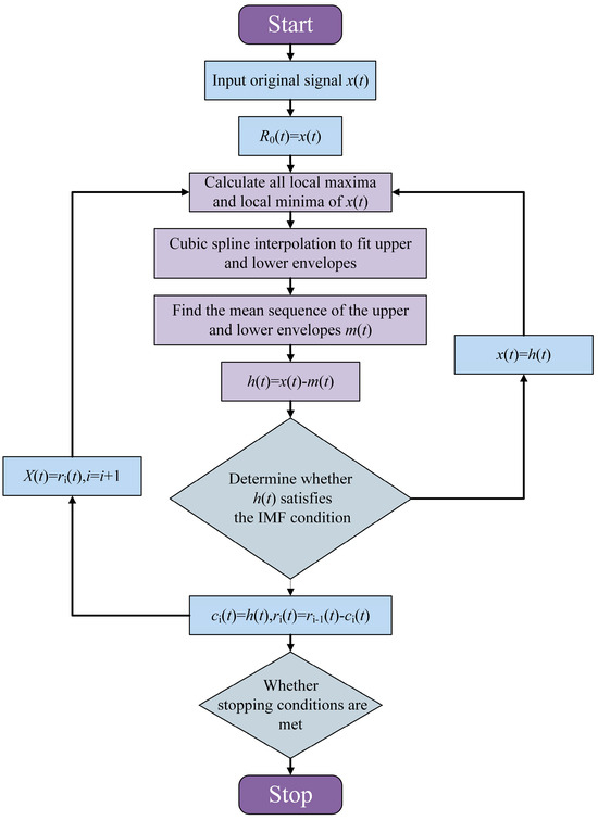
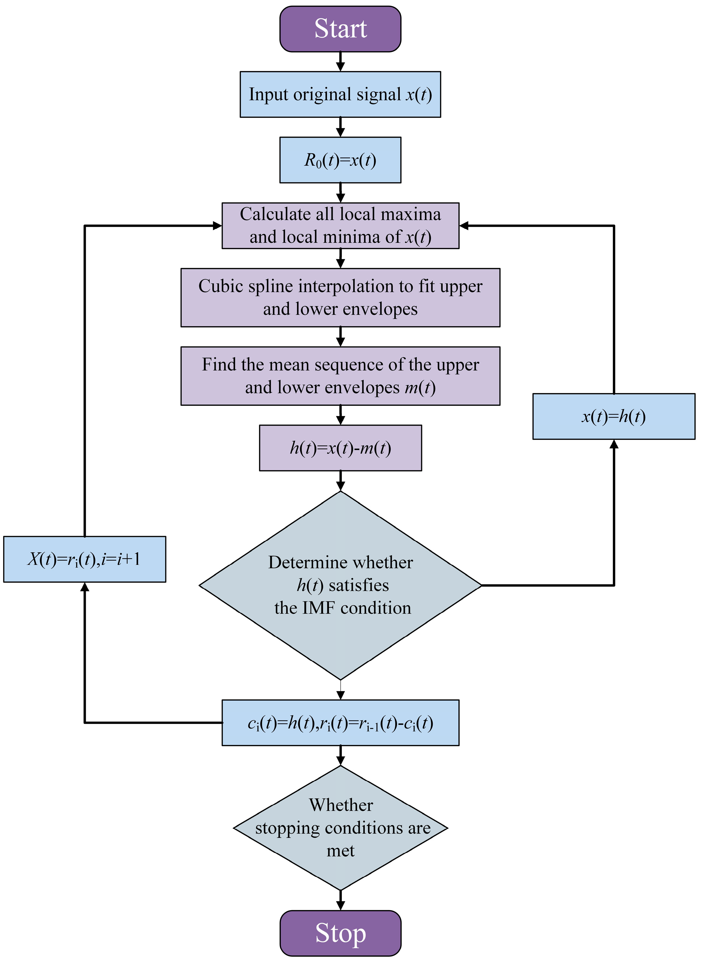
As an adaptive time-frequency analysis method, Empirical Mode Decomposition (EMD)’s core advantage is overcoming the limitations of traditional time-frequency processing techniques (e.g., Fourier transform or wavelet transform) that rely on predefined fixed basis functions. EMD does not require any prior basis function settings or manual parameter adjustments; instead, it performs adaptive decomposition through an iterative sifting process strictly based on the local characteristics of the signal, including local extrema, zero crossings, and local means. This process progressively decomposes the original signal into a set of components, satisfying the criteria of Intrinsic Mode Functions (IMFs)—each IMF must satisfy two conditions: the number of extrema and zero crossings can differ by at most one, and their local mean should be zero—along with a residual component. This data-driven decomposition mechanism, based on the intrinsic local properties of the signal, enables the unbiased and adaptive processing of nonlinear and non-stationary signals without requiring additional preprocessing or manual intervention. Figure 2 presents the EMD flowchart.

Figure 2. EMD flowchart.

As an improved variant of EMD, Ensemble Empirical Mode Decomposition (EEMD) systematically addresses the inherent mode mixing problem in EMD by incorporating white noise-assisted decomposition and multiple statistical averaging mechanisms, thereby significantly enhancing the stability and precision of the noise reduction in time series analyses. In non-stationary signal processing, EMD often suffers from mode mixing due to uneven distributions of local extrema, which causes different frequency components to be mixed within the same IMFs, leading to the distorted separation of effective signals and noise. EEMD mitigates this limitation by introducing random white noise into the original signal, forcing multi-scale components of the signal to disperse into independent IMFs during repeated EMDs. Subsequently, statistical averaging across multiple trials cancels out the random noise while preserving genuine signal characteristics, effectively suppressing mode mixing. This mechanism not only ensures statistical consistency in decomposition results but also enhances robustness in high-noise environments. Consequently, EEMD provides reconstructed signals with higher signal-to-noise ratios and clearer feature representations, offering a more reliable foundation for subsequent analysis. The steps of the EEMD algorithm can be summarized as follows:

Step 1: Add a set of white noise sequences n_i(t) that satisfy the standard normal distribution to the original signal x(t) to obtain a new signal x_i(t):

$${\mathrm{x}}_i\left(t\right)=\mathrm{x}\left(t\right)+n_i\left(t\right)$$

(1)

Step 2: Perform EMD on the new signal x_i(t) introduced with white noise to obtain a set of IMF components and corresponding residual terms.

Step 3: Repeat steps 1 and 2 to integrate and average all IMFs to obtain the final decomposition result:

$$IM{F}_k\left(t\right)={\displaystyle \frac{1}{N}}{\displaystyle \sum _{i=1}^{N}IM{F}_i^k\left(t\right)}$$

(2)

2.2. TiDE

TiDE is an MLP-based encoder–decoder architecture specifically designed for efficiently addressing long-term time series forecasting tasks. By avoiding the use of self-attention, recurrent, or convolutional mechanisms, the model achieves a linear relationship between computational complexity and sequence length. This design enables TiDE to effectively handle covariates and nonlinear dependencies while significantly reducing the computational overhead. As a result, TiDE combines computational efficiency with strong model expressiveness in long-term time series prediction scenarios.

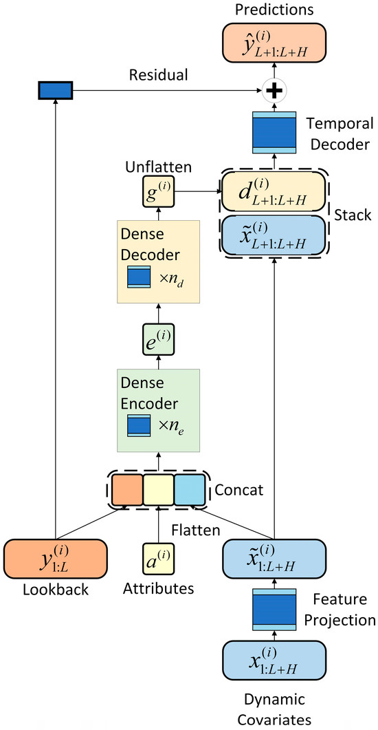
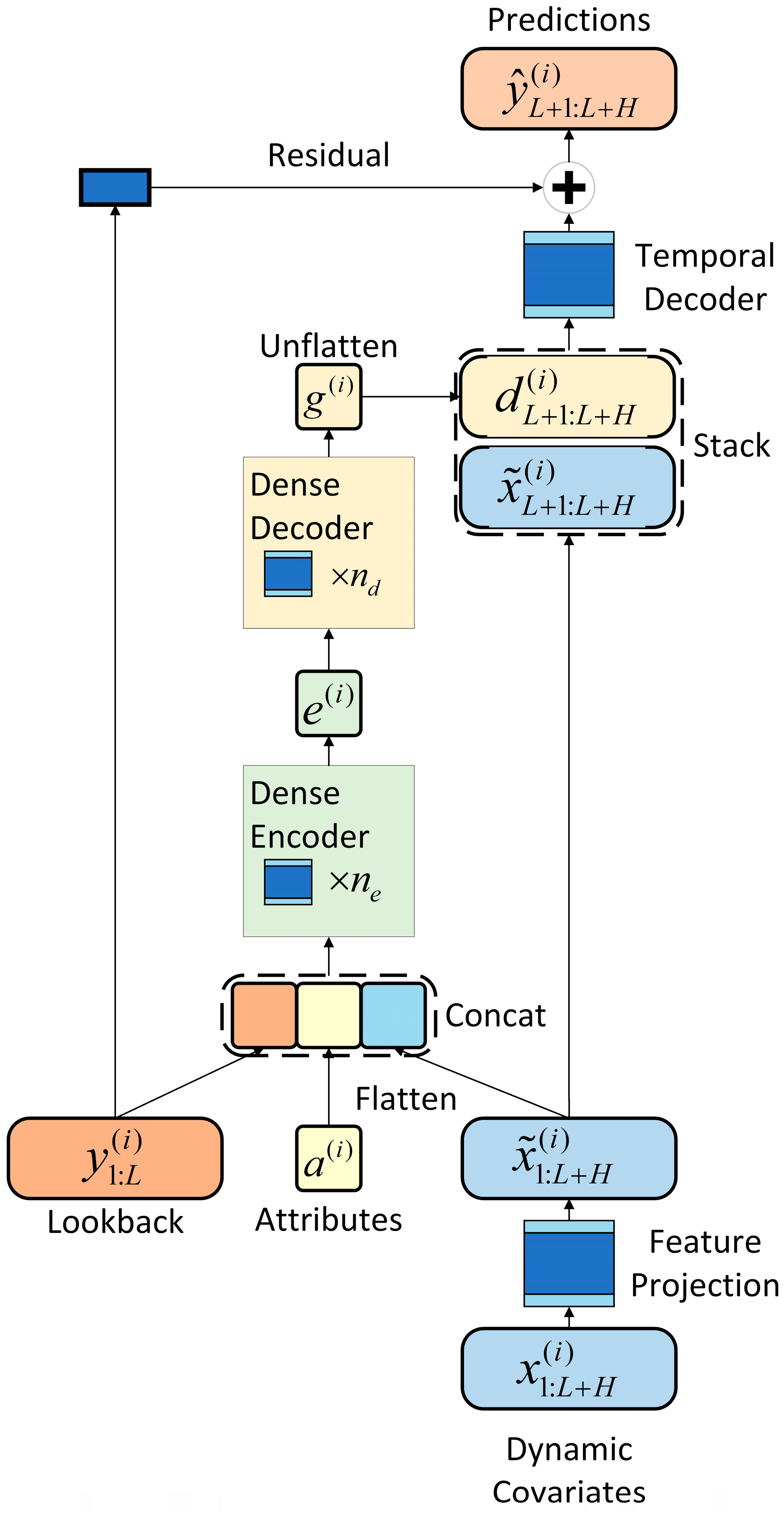
During the encoding phase, TiDE employs cross-dimensional feature fusion to coherently integrate historical time series observations, historical temporal features, future temporal indicators, and passenger flow dynamics into a unified latent representation. The encoder subsequently projects this representation into a multi-step forecasting manifold, while the decoder leverages future temporal features to generate precise multi-step predictions, thereby substantially enhancing forecasting accuracy through synergistic feature integration. As the architectural cornerstone, residual blocks serve as hierarchical feature extractors within the encoder–decoder framework: they utilize ReLU activation functions and incorporate dropout-regularized linear layers to bolster model generalization capacity. Crucially, residual connections directly concatenate outputs with inputs to mitigate gradient explosion and accelerate convergence by preserving an unimpeded gradient flow. Finally, hidden layer weights undergo layer normalization to ensure stable training dynamics and optimal convergence efficiency, establishing a robust foundation for high-precision long-horizon forecasting. Figure 3 displays the TiDE architecture.

Figure 3. The TiDE structure.

The Dense Encoder’s core functionality is mapping historical observations of time series data and their associated covariates into compact representations within a high-dimensional feature space. The encoding process comprises two fundamental stages: feature projection and dense encoding. During the feature projection phase, residual blocks are employed to transform the input vector x_t⁽ⁱ⁾ at each temporal step (encompassing both historical and future horizons) into low-dimensional projections of dimension $\tilde{r}\ll r$, where $\tilde{r}$ denotes the projected feature dimensionality, and r represents the original input dimensionality. This procedure can be expressed using Equation (3). In the dense encoding phase, the feature projections of dynamic covariates are first flattened and subsequently concatenated with static attributes and historical time series features to form the input for dense encoding. These composite features are then fed into an encoder architecture comprising multiple residual blocks. This procedure can be expressed using Equation (4).

$${\tilde{x}}_t^{(i)}=ResidualBlock(x_t^{(i)})$$

(3)

$$e^{(i)}=Encoder(y_{1:L}^{(i)};x_{1:L+H;}^{(i)};a^{(i)})$$

(4)

The core objective of the decoding phase in TiDE is to map the hidden states generated by the encoder into predictive sequences for future time series. This phase comprises two key components: the dense and the temporal decoder. The dense decoder is constructed by stacking multiple residual blocks. This module takes the encoded representation e⁽ⁱ⁾ as the input and transforms it into a vector g⁽ⁱ⁾ with a size of H $\times$ p, where p denotes the output dimension of the decoder. Subsequently, the vector g⁽ⁱ⁾ is reshaped into a matrix structure of $D^{(i)}\in R^{p\times H}$, where the t column d_t⁽ⁱ⁾ represents the decoding vector corresponding to the t time step in the multi-step prediction horizon. This procedure can be expressed using Equations (5) and (6). The temporal decoder maps the output of the dense decoder to the final time series predictions. It concatenates the decoding vector d_t⁽ⁱ⁾ for the prediction time step t with the covariate projection ${\tilde{x}}_{L+t}^{(i)}$ and then transforms this composite input through a residual block to generate the final prediction ${\widehat{y}}_{L+t}^{(i)}$, which can be computed using Equation (7).

$$g^{(i)}=Decoder(e^{(i)})\in R^{H\times p}$$

(5)

$$D^{(i)}=Reshape(g^{(i)})\in R^{p\times H}$$

(6)

$${\widehat{y}}_{L+t}^{(i)}=TemporalDecoder({d_t}^{(i)};{\tilde{x}}_{L+t}^{(i)})$$

(7)

Finally, the model incorporates a global residual connection that linearly projects the retrospective component $y_{1:L}^{(i)}$ into a vector with identical temporal dimensionality to the prediction horizon. This projected vector is then added to the intermediate predictions ${\widehat{y}}_{L+1:L+H}^{(i)}$, yielding the final forecasting output.

2.3. EEMD-TiDE

The EEMD-TiDE model comprises two core stages—data decomposition and forecasting—as illustrated in Figure 1. In the decomposition phase, the Ensemble Empirical Mode Decomposition (EEMD) algorithm is employed to decompose the original passenger flow time series, yielding a set of Intrinsic Mode Functions (IMFs) ordered from high to low frequency along with a residual term. Subsequently, during the prediction phase, each IMF is individually fed into the TiDE (Time Series Dense Encoder) model for independent forecasting. TiDE, an encoder–decoder architecture based on Multi-Layer Perceptron (MLP), is specifically designed for long-term time series forecasting tasks. This model effectively integrates the computational efficiency of linear models with the capability to capture nonlinear dependencies, while also accommodating covariate information. Notably, the simplified linear variant of TiDE can achieve near-optimal forecasting performances for Linear Dynamic Systems (LDSs) under specific conditions. Finally, the overall forecasting result of the EEMD-TiDE model is obtained by aggregating the individual predictions of all IMF components through summation. The EEMD-TiDE framework achieves an optimal balance between accuracy and computational efficiency through a carefully designed dual-stage architecture. Its total time complexity is O(N² + L·H), where O(N²) (N = sequence length) represents the one-time EEMD (performed offline during data preprocessing), and O(L·H) (L = lookback window, H = prediction horizon) denotes the TiDE prediction phase. Crucially, the EEMD preprocessing step—while theoretically O(N²)—is executed only once and does not affect real-time predictions, causing the operational runtime to be dominated by TiDE’s highly efficient O(L·H) predictions.

3. Experiments

3.1. Dataset

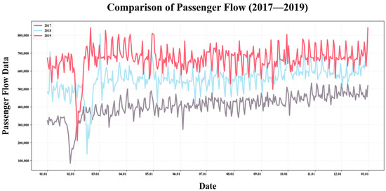
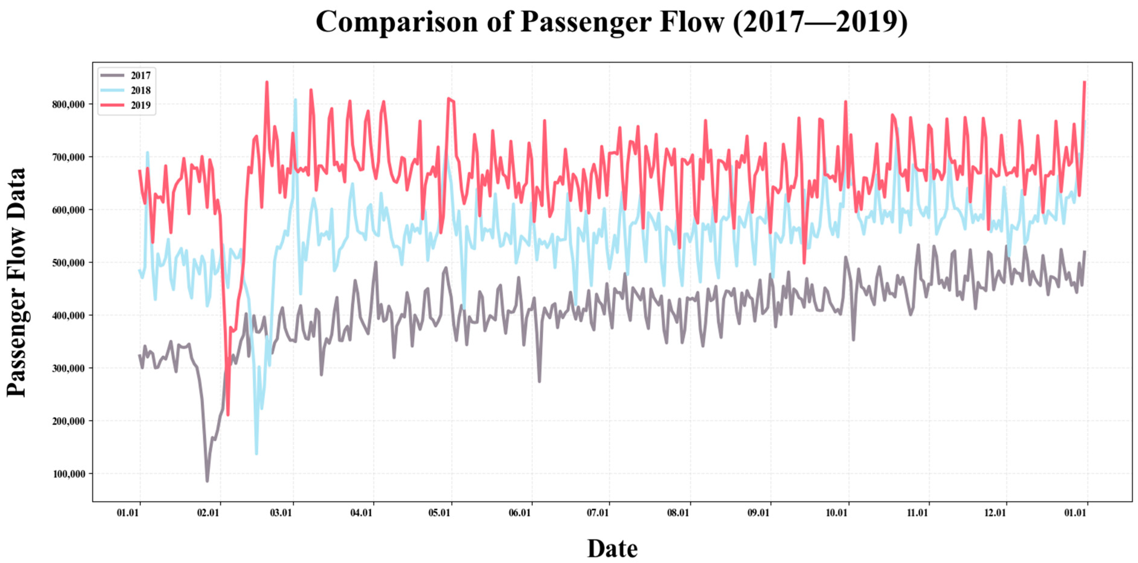
In this study, the proposed EEMD-TiDE model was validated using operational data from Xi’an Metro. The dataset, provided by Xi’an Rail Transit Group Co., Ltd. (Xi’an, China), spans operational records from 1 January 2017 to 31 December 2019 and consists of passenger flow data from 26 stations along a single metro line, totaling 1095 days of inbound passenger flow data. The time granularity is one day. Figure 4 presents the passenger flow data. To ensure robustness and prevent temporal leakage, the dataset was strictly partitioned into training (70%), validation (15%), and testing (15%) subsets in chronological order (i.e., the first 70% of the data was used for training, the subsequent 15% was used for validation, and the final 15% was used for testing). EEMD is strictly confined to the training set, with the test set and validation set not participating in any preprocessing. Prior to model training, data normalization was performed, and variables with differing magnitudes were standardized to enhance the model’s generalization capability. To accurately predict abrupt fluctuations in passenger flow, we specifically annotated holiday data within the dataset. The weekly periodic patterns were directly obtained from standard calendars, with Monday through Sunday representing the recurring weekly structure. In China, weekends (Saturday and Sunday) are classified as regular holidays. Additionally, specific public holidays were identified using the “Chinese Calendar 1.11.0” Python package. Binary indicators (0–1 variables) were employed to encode both the day-of-the-week and holiday status. Consequently, the final input dataset achieved a dimensionality of 1095 × 10.

Figure 4. The passenger flow data.

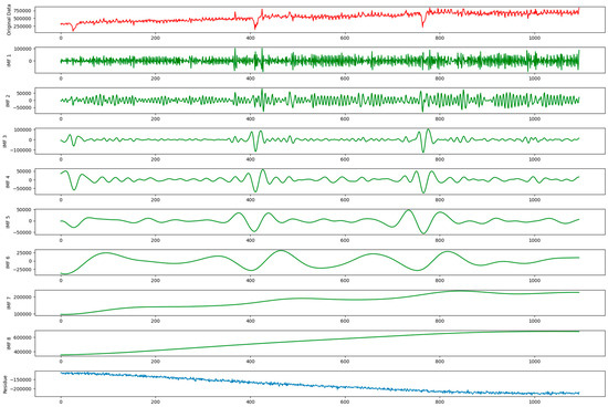
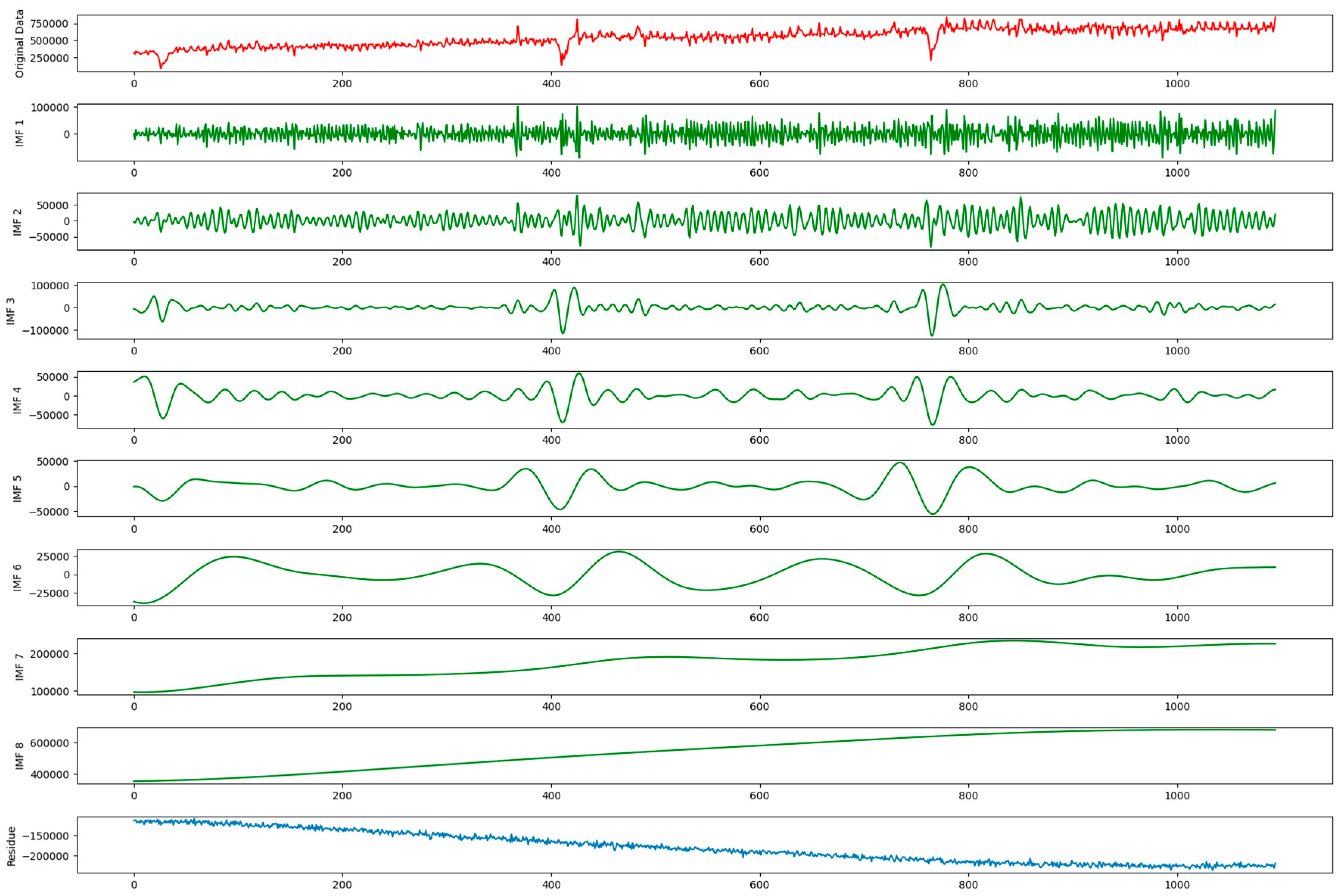
Using the EEMD algorithm, we decomposed the passenger flow data into multiple Intrinsic Mode Functions (IMFs) and a residual component. Figure 5 presents the EEMD results of the passenger flow data from Xi’an Metro between 2017 and 2019, resulting in eight IMFs and one residual component. These IMFs are systematically ordered by frequency, ranging from high to low: high-frequency IMFs (IMF₁–IMF₂) primarily capture short-term high-frequency oscillations and potential noise components, reflecting rapid between-day fluctuations; medium-frequency IMFs (IMF₃–IMF₆) characterize systematic fluctuations at intermediate temporal scales, encompassing the weekly periodicity (e.g., weekday–weekend disparities) and seasonal variations at monthly or quarterly resolutions (e.g., regular patterns in consumption behavior or economic activity); and low-frequency IMFs (IMF₇–IMF₈) represent the long-term trend component, delineating the overall growth or decay trajectory of the data (e.g., annual upward trends or structural shifts). In this study, the standard deviation for noise was set to 0.2, the ensemble size was 100, and the extreme detection method adopted the “parabol” algorithm. These critical parameters collectively determine the effectiveness and computational efficiency of the EEMD. Other parameters, such as the stopping criterion and the maximum number of siftings, were utilized according to the default settings provided by the EMD-Signal 1.40.

Figure 5. The results of the EEMD.

3.2. Model Configurations and Evaluation Metrics

In this study, the model’s hyperparameters include the number of hidden units, batch size, and learning rate. Based on preliminary experimental results, the hidden unit count required to achieve optimal performance was determined to be 128. The batch size was established as 32 from the candidate set {16, 32, 64, 128}, balancing computational efficiency and convergence speed. Through multiple rounds of hyperparameter tuning experiments, the learning rate was optimized to 0.001 as the most effective value. The training process was conducted over 30 epochs to ensure sufficient learning. To enhance the generalization capability, a dropout rate of 0.05 was applied during training. Model parameters were optimized using the Adam optimizer, selected for its robustness in addressing gradient vanishing and exploding gradient problems. The training objective was to minimize the mean squared error (MSE), a standardized metric for evaluating prediction accuracy, achieved through the backpropagation algorithm, which dynamically adjusts model weights to minimize prediction errors.

$$MSE={\displaystyle \frac{1}{N}}{\displaystyle \sum _{i=1}^N{(y_i-{\widehat{y}}_i)}^2}$$

(8)

In this paper, the root mean square error (RMSE), mean absolute error (MAE), and mean absolute percentage error (MAPE) are used as the assessment criteria to evaluate the performance of the proposed hybrid model:

$$RMSE=\sqrt{{\displaystyle \frac{1}{N}}{\displaystyle \sum _{i=1}^N{\left(y_i-{\widehat{y}}_i\right)}^2}}$$

(9)

$$MAE={\displaystyle \frac{1}{N}}{\displaystyle \sum _{i=1}^N\left|y_i-{\widehat{y}}_i\right|}$$

(10)

$$MAPE={\displaystyle \frac{1}{N}}{\displaystyle \sum _{i=1}^N\left|\frac{y_i-{\widehat{y}}_i}{y_i}\right|}\times 100\%$$

(11)

where y_i is the real value, ${\widehat{y}}_i$ is the predicted value, and N is the length of data.

3.3. Baseline Models

To validate the performance of the proposed EEMD-TiDE model, we conducted comparative evaluations against several well-established benchmark models. Additionally, to ensure methodological rigor, Table 1 provides a comprehensive characterization of the software and computational environment.

Table 1. Hardware and compiling environment.

Categories	Version
Central Processing Unit (CPU)	13th Gen Intel(R) Core(TM) i7-13620H 2.40 GHz
Operating System (OS)	Windows 11 Professional x64
Random Access Memory (RAM)	16.0 GB
Graphics Processing Unit (GPU)	NVIDIA GeForce GTX 4060 8 GB
Programming Language	Python 3.9.18
Development Environment	VSCode 1.84.1
	CUDA 12.1
Main Python Modules	PyTorch 2.3.0
	EMD-signal 1.4.0
	NumPy 1.26.4
	Pandas 1.5.3
	Matplotlib 3.8.3

• ARIMA: The Autoregressive Integrated Moving Average (ARIMA) model is a classical linear method used for time series forecasting. It is defined by three key parameters: the autoregressive order (pp), the differencing order (dd), and the moving average order (qq). Optimal parameter selection is achieved using the Akaike Information Criterion (AIC), balancing predictive accuracy and model complexity. Its parameters are configured as follows: the lag order is set to 2, the degree of difference is 1, and the order of moving averages is also 1.
• LSTM: Long Short-Term Memory, a variant of recurrent neural networks (RNNs), employs collaborative mechanisms of input, forget, and output gates to effectively capture long-term dependencies in sequential data. This architecture mitigates gradient vanishing issues, enabling the stable processing of temporal sequences and achieving high precision in complex forecasting tasks. In this model, there is one fully connected layer accompanied by two hidden layers. The hidden states are configured with a dimension of 128, while the fully connected layer comprises 64 neurons.
• GRU: The Gated Recurrent Unit simplifies the LSTM architecture by merging the input and forget gates into a single update gate and eliminating the separate cell state. This structural optimization reduces both the parameter count and computational complexity while preserving the ability to model long-term dependencies, thereby enhancing training efficiency and inference speed. In this model, there is one fully connected layer accompanied by two hidden layers. The hidden states are configured with a dimension of 128, while the fully connected layer comprises 64 neurons.
• TCN: The Temporal Convolutional Network utilizes dilated convolutional layers to parallelize temporal data processing, enabling the efficient capture of long-range dependencies through stacked convolutional structures. Unlike traditional RNNs, the TCN avoids sequential computation bottlenecks, offering superior computational efficiency for large-scale time series forecasting. In this model, there is one fully connected layer accompanied by two hidden layers. The hidden states are configured with a dimension of 128, while the fully connected layer comprises 64 neurons. Meanwhile, the number of channels of the TCN is [64, 128, 256], and the convolutional kernel size is 3.
• Transformer: The Transformer architecture leverages an encoder–decoder framework combined with self-attention mechanisms to dynamically weight the importance of different temporal positions in input sequences. This adaptive weighting mechanism enables the robust modeling of long-term dependencies and exceptional contextual understandings, making it highly effective for the high-precision forecasting of complex temporal patterns. In this model, the conventional Transformer is composed of three encoder layers and three decoder layers, each equipped with eight multi-head attention mechanisms. The dimensions for d_k and d_v are both configured to be 64. Following the Transformer’s output, it is fed into two fully connected layers, the first with 128 neurons and the second with 64 neurons.
• Informer: The Informer is an innovative variant of the Transformer model, specifically designed for long-sequence time series prediction tasks. It introduces a sparse probabilistic self-attention mechanism, which significantly reduces the computational complexity from O(L²) to O(L log L), effectively minimizing both the computation and memory usage during the processing of extended sequences. Furthermore, the Informer employs a self-attention distillation technique that optimizes the allocation of computational resources and memory consumption for long sequences by emphasizing the most salient attentional patterns. This approach contrasts with traditional step-by-step decoding methods, as the Informer’s generative decoder can predict entire sequences in a single pass, thereby markedly enhancing the inference speed. These enhancements enable the Informer to perform better than existing methods across multiple large-scale datasets. The parameters of the Informer are the same as the Transformer.

3.4. Prediction Performance

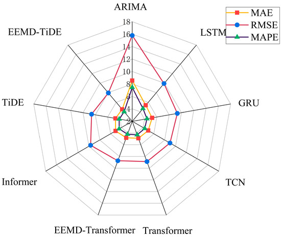
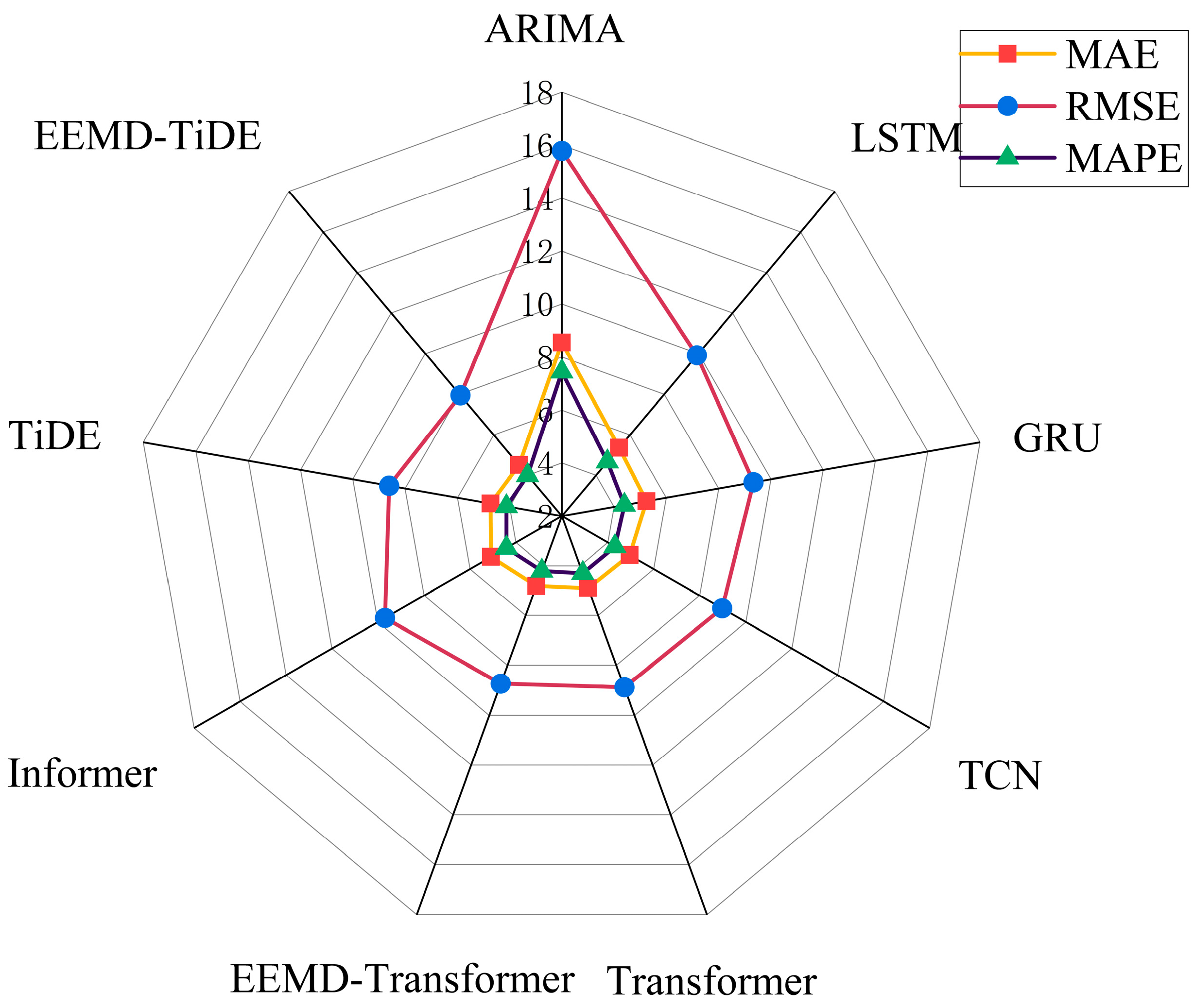
To systematically evaluate the effectiveness of the proposed EEMD-TiDE model in urban rail transit passenger flow forecasting, this study established a comparative experimental framework by selecting five representative forecasting models, which include ARIMA, LSTM, GRU, TCN, and Transformer models as benchmarks for the performance analysis. Table 2 and Figure 6 present the quantitative MAE, RMSE, and MAPE metrics across different prediction models, with the optimal performance values highlighted in bold. The experimental results demonstrate that the EEMD-TiDE model achieves statistically significant superiority over all benchmark models in all prediction horizons. Specifically, compared to the best-performing baseline model (Transformer), the TiDE model achieved reductions of 3.3%, 3.0%, and 3.0% for the MAE, RMSE, and MAPE, respectively. Upon incorporating the EEMD signal decomposition mechanism, the EEMD-TiDE model demonstrated a significantly enhanced performance, with average reductions of 7.8%, 10.0%, and 6.7% for the MAE, RMSE, and MAPE, respectively. These results validate the superior capability of the hybrid model at capturing complex temporal patterns inherent in urban passenger flow dynamics.

Table 2. Performance comparison of different models.

Model	MAE	RMSE	MAPE
ARIMA	8.549	15.783	7.447
LSTM	5.364	9.917	4.672
GRU	5.237	9.328	4.391
TCN	4.948	8.972	4.313
Transformer	4.895	8.882	4.294
EEMD–Transformer	4.801	8.733	4.203
Informer	5.085	9.693	4.413
TiDE	4.732	8.612	4.118
EEMD-TiDE	4.513	7.951	4.003

Figure 6. Performance comparison of different models.

The experimental results indicate that the TiDE model outperforms all baseline models across all evaluation metrics, as demonstrated by its MAE of 4.732, RMSE of 8.612, and MAPE of 4.118. The EEMD-TiDE model, integrated with the EEMD technique, achieves further improvements in prediction accuracy, yielding the following optimized performance metrics: an MAE of 4.513, an RMSE of 7.951, and an MAPE of 4.003. A quantitative analysis confirms the effectiveness of the time series decomposition mechanism, revealing that models incorporating EEMD demonstrate statistically significant superiority over baseline models without decomposition. These findings suggest that extracting latent feature components through EEMD substantially enhances the predictive performance in complex nonlinear time series forecasting tasks. Particularly in urban rail transit passenger flow prediction scenarios, multi-scale feature separation plays a critical role in modeling the underlying dynamic patterns of intricate transportation systems.

Compared to other models, the traditional linear ARIMA model demonstrates significant limitations in capturing the evolutionary characteristics of the passenger flow, indicating its inadequacy in characterizing complex temporal dependencies. In contrast, gated recurrent neural networks (LSTM and GRU) exhibit notable advantages: LSTM effectively models long-term dependencies through memory cells, while its variant, the GRU, achieves a comparable performance with more efficient parameter configuration, even surpassing LSTM in certain experimental scenarios.

In the domain of sequence modeling, the TCN has emerged as a formidable competitor through its distinctive architectural design. By stacking dilated convolution layers, TCNs achieve parallel processing capabilities for long sequences, demonstrating a computational efficiency that is 2–3 orders of magnitude higher compared to RNN models that rely on sequential processing, while maintaining robust generalization performance.

Additionally, the Transformer employs multi-head self-attention to capture multiple temporal dependencies, thereby enhancing prediction accuracy. However, its applicability for long-term sequence processing is limited by storage constraints imposed by the stacked layers when handling lengthy inputs. To address this limitation, the Informer introduces a novel probabilistic sparse attention mechanism designed to maintain a strong predictive performance while significantly reducing computational and storage requirements. Nevertheless, both the Transformer and Informer may exhibit sensitivity to minor variations in input data, which could lead to substantial output fluctuations and potentially compromise the stability of prediction results in certain scenarios.

Experimental results demonstrate that the TiDE model achieves optimal performance across all evaluation metrics. The TiDE model effectively addresses the challenge of modeling nonlinear dependencies by employing feature projection techniques to map both static and dynamic covariates into a high-dimensional feature space. Its densely connected encoder–decoder architecture circumvents the computational overhead associated with self-attention mechanisms. Specifically, TiDE achieves improvements that are 5–10 times greater in both training and inference efficiency compared to conventional Transformers, primarily due to its abandonment of the self-attention mechanism (with computational complexity O(n²)) in favor of an MLP-based encoder–decoder architecture (with linear complexity O(n)). The self-attention mechanism in Transformers requires the computation of the QKᵀ matrix, which accounts for over 70% of their computational load. As the sequence length n increases, computational demands grow quadratically. In contrast, TiDE maintains linear computational complexity (O(n)) through its dense MLP encoder and residual block structures, significantly enhancing its efficiency for long-sequence forecasting tasks. Furthermore, TiDE achieves a comparable performance to a six-layer Transformer using only four layers, while requiring fewer parameters (approximately 49 K vs. 65 K). This architectural simplification reduces FLOPs from 7.2 M to 1.2 M while preserving high prediction accuracy and enabling the computational efficiency required for industrial deployment. Although EEMD effectively decomposes the original signal, the self-attention mechanism of the Transformer is prone to high-frequency noise interference when processing the decomposed IMF components, resulting in limited improvements in prediction accuracy when combined with EEMD. In contrast, the EEMD-TiDE model employs a feature projection step to map covariates and historical sequences into a low-dimensional space, effectively filtering high-frequency noise and reinforcing key dependency relationships, thereby enabling the model to precisely focus on the core patterns that drive accurate predictions. Meanwhile, peak periods (e.g., holiday seasons) typically exhibit strong non-stationarity, characterized by abrupt passenger flow fluctuations and overlapping multi-peak patterns that induce systematic prediction biases in conventional models. In contrast, off-peak periods (e.g., weekdays) demonstrate relatively stable and periodic flow patterns, which are easier for models to capture. The EEMD-TiDE framework inherently resolves this dichotomy through its dual-stage architecture: EEMD decomposes mixed traffic signals into physically meaningful IMF components, isolating transient fluctuations during peak periods and baseline trends during off-peak periods. Subsequently, TiDE’s channel-independent prediction mechanism performs adaptive modeling for each component. This design enables the model to mitigate the prediction distortion caused by signal non-stationarity during peak periods while preserving high-precision pattern capture for regularities in off-peak periods. Consequently, the integrated forecasting framework achieves a uniform error distribution—which is neither significantly distorted by the peak period’s volatility nor oversimplified by off-peak periodicity—ultimately demonstrating a robust performance in holistic predictions decoupled from temporal characteristics. Notably, when integrated with EEMD as a preprocessing step, TiDE’s predictive accuracy is significantly enhanced, validating its superior adaptability in complex time series modeling tasks.

To determine which models achieved high-quality results, we conducted paired t-tests on the MAE, RMSE, and MAPE metrics of all proposed models at a 5% significance level. The null hypothesis in this study posits that there is no statistically significant difference in these metrics between any two models. If the p-value derived from the t-test falls below 0.05, the null hypothesis is rejected. Table 3 presents the results of the t-test, with p-values less than 0.05 in most cases.

Table 3. p-values of paired t-test.

Model	MAE	RMSE	MAPE
ARIMA and LSTM	0.0003	0.0472	0.0124
ARIMA and GRU	0.0283	0.0013	0.0101
ARIMA and TCN	0.0482	0.0456	0.0283
ARIMA and Transformer	0.0143	0.0421	0.0184
ARIMA and EEMD–Transformer	0.0143	0.0335	0.0471
ARIMA and Informer	0.0352	0.0105	0.0384
ARIMA and TiDE	0.0402	0.0173	0.0205
ARIMA and EEMD-TiDE	0.0092	0.0076	0.0117
LSTM and GRU	0.0491	0.0702	0.0165
LSTM and TCN	0.0463	0.0278	0.0089
LSTM and Transformer	0.0415	0.0194	0.0247
LSTM and EEMD–Transformer	0.0389	0.0065	0.0423
LSTM and Informer	0.0152	0.0342	0.0480
LSTM and TiDE	0.0686	0.0113	0.0364
LSTM and EEMD-TiDE	0.0256	0.0172	0.0375
GRU and TCN	0.0453	0.0231	0.0124
GRU and Transformer	0.0397	0.0264	0.0183
GRU and EEMD–Transformer	0.0352	0.0430	0.0216
GRU and Informer	0.0473	0.0331	0.0147
GRU and TiDE	0.0442	0.0263	0.0078
GRU and EEMD-TiDE	0.0367	0.0403	0.0176
TCN and Transformer	0.0235	0.0372	0.0059
TCN and EEMD–Transformer	0.0414	0.0245	0.0138
TCN and Informer	0.0146	0.0335	0.0475
TCN and TiDE	0.0276	0.0108	0.0358
TCN and EEMD-TiDE	0.0472	0.0308	0.0124
Transformer and EEMD–Transformer	0.0436	0.0270	0.0080
Transformer and Informer	0.0363	0.0419	0.0485
Transformer and TiDE	0.0297	0.0153	0.0451
Transformer and EEMD-TiDE	0.0264	0.0079	0.0374
EEMD–Transformer and Informer	0.0409	0.0469	0.0323
EEMD–Transformer and TiDE	0.0142	0.0428	0.0255
EEMD–Transformer and EEMD-TiDE	0.0071	0.0357	0.0396
Informer and TiDE	0.0242	0.0162	0.0336
Informer and EEMD-TiDE	0.0410	0.0195	0.0218
TiDE and EEMD-TiDE	0.0105	0.0332	0.0268

4. Conclusions

This study addresses the critical challenge of accurate urban rail transit passenger flow forecasting through the development of a novel hybrid model, EEMD-TiDE. The proposed model integrates the strengths of EEMD for signal decomposition and TiDE for efficient time series forecasting, effectively capturing both short-term fluctuations and long-term trends in complex passenger flow data. The EEMD component overcomes mode mixing limitations of traditional EMD by incorporating white noise perturbations, decomposing the original data into physically meaningful IMF components. The TiDE model, with its linear architecture and support for various covariates, provides computational efficiency while maintaining high predictive accuracy. Extensive experiments on Xi’an Metro data demonstrate that EEMD-TiDE achieves statistically significant improvements over all baseline models. Notably, the model’s ability to handle multiple external variables without high computational costs makes it particularly suitable for real-world transportation systems with complex dynamics. Future work will address this study’s key limitations by extending the model to multi-line networks (to overcome single-line scope constraints), validating across multiple cities (to ensure generalizability), and developing adaptive EEMD parameter selection (to mitigate sensitivity issues). Additionally, integrating contextual factors such as weather and special events will further enhance prediction accuracy.

References

- Li, M.; Zhang, C. An Urban Metro Section Flow Forecasting Method Combining Time Series Decomposition and a Generative Adversarial Network. Sustainability 2024, 16, 607. [Google Scholar] [CrossRef] [Scilit]
- Owais, M.; Allam, A.A. Adaptive Optimization of Traffic Sensor Locations Under Uncertainty Using Flow-Constrained Inference. Appl. Sci. 2025, 15, 10257. [Google Scholar] [CrossRef] [Scilit]
- Wang, X.; Kang, Y.; Hyndman, R.J.; Li, F. Distributed ARIMA models for ultra-long time series. Int. J. Forecast. 2023, 39, 1163–1184. [Google Scholar]
- Zhao, J.; Yu, Z.; Yang, X.; Gao, Z.; Liu, W. Short term traffic flow prediction of expressway service area based on STL-OMS. Phys. A Stat. Mech. Its Appl. 2022, 595, 126937. [Google Scholar] [CrossRef] [Scilit]
- Lin, G.; Lin, A.; Gu, D. Using support vector regression and K-nearest neighbors for short-term traffic flow prediction based on maximal information coefficient. Inf. Sci. 2022, 608, 517–531. [Google Scholar] [CrossRef] [Scilit]
- Yu, B.; Lee, Y.; Sohn, K. Forecasting road traffic speeds by considering area-wide spatio-temporal dependencies based on a graph convolutional neural network (GCN). Transp. Res. Part C Emerg. Technol. 2020, 114, 189–204. [Google Scholar] [CrossRef] [Scilit]
- Yang, H.-F.; Chen, Y.-P.P. Hybrid deep learning and empirical mode decomposition model for time series applications. Expert Syst. Appl. 2019, 120, 128–138. [Google Scholar] [CrossRef] [Scilit]
- Liu, Y.; Wu, F.; Liu, Z.; Wang, K.; Wang, F.; Qu, X. Can language models be used for real-world urban-delivery route optimization? Innovation 2023, 4, 100520. [Google Scholar] [CrossRef] [Scilit] [PubMed]
- Tselentis, D.I.; Vlahogianni, E.I.; Karlaftis, M.G. Improving short-term traffic forecasts: To combine models or not to combine? IET Intell. Transp. Syst. 2015, 9, 193–201. [Google Scholar] [CrossRef] [Scilit]
- Zhang, Y.; Zhang, Y.; Haghani, A. A hybrid short-term traffic flow forecasting method based on spectral analysis and statistical volatility model. Transp. Res. Part C Emerg. Technol. 2014, 43, 65–78. [Google Scholar] [CrossRef] [Scilit]
- Pan, Y.A.; Guo, J.; Chen, Y.; Cheng, Q.; Li, W.; Liu, Y. A fundamental diagram-based hybrid framework for traffic flow estimation and prediction by combining a Markovian model with deep learning. Expert Syst. Appl. 2024, 238, 122219. [Google Scholar] [CrossRef] [Scilit]
- Deng, S.; Du, J.; Zhang, J.; Wang, X. Deep learning approach for short-term entry passenger flow forecasting in urban rail transit stations. Eng. Appl. Artif. Intell. 2026, 163, 112989. [Google Scholar]
- Mao, Y.; Yu, X. A hybrid forecasting approach for China’s national carbon emission allowance prices with balanced accuracy and interpretability. J. Environ. Manag. 2023, 351, 119873. [Google Scholar] [CrossRef] [Scilit] [PubMed]
- Huang, H. Introduction to the Hilbert–Huang Transform And Its Related Mathmatical L Problems. In Hilbert-Huang Transform and Its Applications; World Scientific Publishing: Singapore, 2003; pp. 1–26. [Google Scholar]
- Wei, Y.; Chen, M.-C. Forecasting the short-term metro passenger flow with empirical mode decomposition and neural networks. Transp. Res. Part C Emerg. Technol. 2012, 21, 148–162. [Google Scholar] [CrossRef] [Scilit]
- Yu, X.; Shi, S.; Xu, L. A spatial–temporal graph attention network approach for air temperature forecasting. Appl. Soft Comput. 2021, 113, 107888. [Google Scholar] [CrossRef] [Scilit]
- He, K.; Chen, Y.; Tso, G.K.F. Price forecasting in the precious metal market: A multivariate EMD denoising approach. Resour. Policy 2017, 54, 9–24. [Google Scholar] [CrossRef] [Scilit]
- Cao, J.; Li, Z.; Li, J. Financial time series forecasting model based on CEEMDAN and LSTM. Phys. A Stat. Mech. Its Appl. 2019, 519, 127–139. [Google Scholar] [CrossRef] [Scilit]
- Huang, Y.; Hasan, N.; Deng, C.; Bao, Y. Multivariate empirical mode decomposition based hybrid model for day-ahead peak load forecasting. Energy 2022, 239, 122245. [Google Scholar] [CrossRef] [Scilit]
- Hao, W.; Sun, X.; Wang, C.; Chen, H.; Huang, L. A hybrid EMD-LSTM model for non-stationary wave prediction in offshore China. Ocean Eng. 2022, 246, 110566. [Google Scholar] [CrossRef] [Scilit]
Disclaimer/Publisher’s Note: The statements, opinions and data contained in all publications are solely those of the individual author(s) and contributor(s) and not of MDPI and/or the editor(s). MDPI and/or the editor(s) disclaim responsibility for any injury to people or property resulting from any ideas, methods, instructions or products referred to in the content. |
© 2026 by the authors. Licensee MDPI, Basel, Switzerland. This article is an open access article distributed under the terms and conditions of the Creative Commons Attribution (CC BY) license.