An Ensemble Learning Approach for Wind Power Prediction Using Hybrid Deep Learning

Abstract

Wind power prediction is important for utility grid energy scheduling. However, prediction accuracy suffers from poor data quality and limited feature engineering. Therefore, this paper proposes a data-driven ensemble learning framework to deal with these issues. First, the paper divides raw data into four seasonal groups. A preprocessing pipeline integrating the 3$\sigma$ rule, Hermite interpolation, and a wind power curve modeling method detects and corrects outliers. Second, we develop a two-stage prediction strategy. In the first stage, a hybrid deep learning model including convolutional neural networks, gated recurrent units, and an attention mechanism jointly learns spatio-temporal features, with hyperparameters optimized using the exponential-trigonometric optimization (ETO) algorithm and the input length determined using the partial autocorrelation function. In the second stage, a temporal convolutional network with ETO-optimized hyperparameters predicts the error sequence, capturing multi-scale nonlinear relationships between input features and error dynamics. Experimental results on real-world wind farm data demonstrate that the proposed method achieves a mean RMSE of $5.89\pm 0.11$ MW, MAE of $4.05\pm 0.09$ MW, MAPE of $7.24\pm 0.18\%$, and $R^2$ of $0.928\pm 0.008$ over 50 independent runs. A representative single run achieves an RMSE of $5.89$ MW, MAE of $4.02$ MW, MAPE of $6.9\%$, and $R^2$ of $0.93$.

1. Introduction

The energy system is undergoing a major transformation, with renewable energy sources increasingly displacing fossil fuels in electricity generation portfolios [1]. Wind power has become a leading contributor, with global installed capacity surpassing 900 GW by 2024 [2]. The International Energy Agency reports that wind energy will supply more than 30% of global electricity by 2030, showing its key role in reaching carbon neutrality targets [3]. By 2050, the International Energy Agency’s Net Zero by 2050 roadmap projects that wind and solar PV together will account for nearly 70% of total global electricity generation [4]. However, the inherent intermittency and stochastic variability of wind resources challenge power system operation [5]. As wind power penetration continues to escalate, the room for prediction error narrows, making high-accuracy forecasting not simply a research objective but an operational necessity [6].

Accurate wind power forecasting is also essential for assessing power system adequacy—the ability of the available generation fleet and associated resources to meet electricity demand under expected operating conditions. Adequacy assessments typically rely on probabilistic reliability indices, such as loss of load expectation and expected energy not supplied, to quantify the risk and magnitude of supply shortfalls [7,8]. As wind power penetration grows, the uncertain and time-varying contribution of wind generation makes adequacy evaluation more complex than that of conventional dispatchable units. In particular, seasonal and interannual variations in wind energy yield, together with the possible coincidence of low wind generation and high demand, can significantly affect the effective capacity contribution of wind farms and the estimated adequacy level [7,9]. Forecast errors further propagate into estimates of available supply and adequacy margins, increasing the risk that reliability assessments may overstate or understate the contribution of wind generation [8,10]. Improving wind power forecasting accuracy is therefore critical for providing more dependable inputs to adequacy-related decision-making and for supporting reliable operation of high-renewable power systems.

Because wind power generation is inherently variable and strongly dependent on meteorological conditions, deviations between forecasted and actual output can create imbalances between electricity supply and demand, complicating unit commitment, economic dispatch, reserve allocation, energy storage coordination, and transmission congestion management. Overestimating wind generation may require additional spinning reserves or conventional generation to maintain reliability, whereas underestimating it can lead to unnecessary generator commitment, higher operating costs, and avoidable renewable curtailment. These effects are particularly pronounced in systems with high wind power penetration, where forecasting accuracy directly influences operational flexibility and renewable integration [7,8,9]. The economic and operational implications of forecasting inaccuracies are considerable. Overestimating wind power output requires costly spinning reserves to maintain grid reliability, while undervaluing it leads to curtailment of renewable generation and missed revenue opportunities [11]. The economic consequences are substantial: for a 100 MW wind farm, a 10% improvement in prediction accuracy can yield annual savings exceeding 1.5 million in reserve costs and penalty avoidance [12]. Consequently, wind power prediction has attracted intensive research attention across academic and industrial fields over the past two decades.

To improve wind power forecasting accuracy, various statistical, machine learning, and deep learning approaches have been developed. Traditional time-series models, such as autoregressive integrated moving average (ARIMA), and machine learning methods provide useful solutions for modeling historical patterns and nonlinear relationships in wind-related data [13,14]. With the development of deep learning, recurrent neural networks, particularly long short-term memory (LSTM) networks and gated recurrent units (GRUs), have been widely applied to capture temporal dependencies in wind power sequences. CNN-based models can extract local patterns from time-series data, while hybrid CNN–LSTM architectures combine local feature extraction with temporal modeling [15,16]. Furthermore, attention mechanisms enhance forecasting by assigning different weights to historical observations, and Transformer-based architectures can capture long-range dependencies through self-attention [17,18,19,20]. Temporal convolutional networks (TCNs) have also emerged as an alternative for sequence modeling, offering causal convolutions and expanded receptive fields for capturing temporal patterns [21,22,23,24]. More recently, hybrid and ensemble approaches have combined multiple modeling techniques to exploit their complementary strengths and improve prediction performance [16,25,26,27,28]. Despite these advances, accurately forecasting wind power remains challenging because of the stochastic variability of wind resources, complex nonlinear relationships, data quality problems, and the difficulty of simultaneously capturing different temporal patterns.

We identify three obstacles that compromise prediction performance:

• Data Quality Degradation. Wind farm supervisory control and data acquisition (SCADA) systems function as the data source for prediction models. However, these data might be contaminated by multiple quality issues. Sensor drift and malfunction, as well as communication interruptions, introduce outliers, missing values, and measurement noise into the data flows [29]. SCADA datasets reportedly contain anomalous observations, which skew model training and degrade predictive performance [30]. Traditional preprocessing approaches often fail to distinguish true irregularities from event-related disturbances, causing either insufficient data cleaning or the discarding of valuable information.
• Suboptimal Feature Construction. Many existing strategies rely on single-source inputs or do not capture the spatio-temporal dependencies intrinsic to wind generation processes [31]. Wind power output is governed by elaborate interactions among multiple meteorological variables (e.g., wind speed, wind direction, temperature, air density, and turbulent intensity). The meteorological variables exhibit strongly nonlinear and non-stationary characteristics [32]. Simple feature encodings struggle to represent the multi-scale dynamics, causing prediction biases.
• Model Construction Limitations. Deep learning models offer powerful representational capabilities yet are sensitive to architectural design and tuning configuration. Manual adjustment is inefficient and ineffective, while exhaustive grid search is computationally impractical [33]. The lack of optimization methods for model parameters represents a gap, leaving predictive performance untapped [25]. Furthermore, single-prediction models cannot entirely capture the spectrum of data complexities during regime changes.

Compared with the forecasting of other atmospheric variables, such as temperature and atmospheric pressure, wind resource forecasting presents several distinctive challenges. Wind speed and direction can exhibit rapid fluctuations and strong spatial and temporal variability due to atmospheric turbulence, changing weather conditions, and terrain effects. These characteristics make wind forecasting particularly sensitive to the accuracy and resolution of meteorological observations and numerical weather prediction models [34,35]. Furthermore, wind power forecasting is more complex than wind speed prediction alone because the conversion of wind speed into electrical power follows a nonlinear turbine power curve, with cut-in, rated, and cut-out operating regions. Consequently, even relatively small wind speed prediction errors can lead to substantial power output errors under certain operating conditions [36,37]. In addition, turbine availability, wake effects, curtailment, and measurement uncertainty can further complicate the relationship between meteorological conditions and actual wind power generation [35,36]. These uncertainties may propagate through the forecasting process, from weather prediction to power generation estimation, making accurate wind power forecasting a challenging task [35]. These characteristics highlight the need for forecasting methods capable of capturing complex nonlinear relationships and temporal dependencies while remaining robust to data variability and uncertainty.

To address the above issues, we propose a data-driven ensemble learning framework with the following contributions:

• A seasonal data division strategy is combined with an outlier detection and correction pipeline that integrates the 3$\sigma$ rule, wind power curve modeling, and Hermite interpolation. This approach tackles data quality issues whilst preserving physical coherence.
• We employ a two-stage strategy. The first stage establishes a spatio-temporal prediction using CNN-GRU-AM. The second stage corrects errors using a TCN.
• The exponential-trigonometric optimization (ETO) algorithm automatically optimizes hyperparameters for both prediction stages. ETO’s balanced exploration–exploitation mechanism can handle complex engineering optimization problems.
• The partial autocorrelation function (PACF) utilizes a formal approach to determine the optimal historical input window.

The rest of this paper is as follows. Section 2 presents the related work. The background of wind power prediction is given in Section 3. The framework for wind power prediction is provided in Section 4. Section 5 proposes the two-stage wind power prediction approach. The experimental results are shown in Section 6. Section 7 concludes the paper.

2. Related Work

2.1. Deep Learning for Wind Power Prediction

Recent years have witnessed progress in applying deep learning to wind power forecasting. Recurrent neural networks (RNNs) successfully capture time-based relationships in wind power time series [38]. Long short-term memory’s (LSTM’s) memory cells enable selective retention and forgetting of information across long sequences, while GRU offers comparable performance with lower computational complexity [13]. Demirtop et al. [14] demonstrated that stacked LSTM models outperformed autoregressive integrated moving average (ARIMA) models for wind speed prediction. However, RNN-based strategies meet challenges with gradient propagation in long sequences and with processing multivariate spatial correlations.

Convolutional neural networks (CNNs) are used to extract local spatial features from multivariate inputs [39]. The CNN’s ability to locate patterns throughout multiple features makes it a natural choice for initial feature extraction in prediction pipelines. Debnath et al. [15] used a one-dimensional CNN for wind power prediction to capture local patterns in the temporal dimension. Architectures combining CNNs with RNNs have demonstrated potential in jointly learning spatial and temporal representations. Abou et al. [16] proposed a CNN-LSTM model that derives spatial attributes using CNN layers and then extracts temporal connections with LSTM.

Attention is a powerful mechanism that enables selective concentration on the most relevant input segments [40]. In time series forecasting, attention models adaptively weight input sequence elements based on their relevance to the prediction target. For wind power forecasting, attention-weighted GRU or LSTM models show good performance through dynamically emphasizing time steps in the input sequence [17]. Niu et al. [18] incorporated a dual-stage attention mechanism into an LSTM network, achieving a MAPE reduction compared to a non-attentive LSTM. The self-attention module used in Transformer architectures [19] captures distant dependencies. Mo et al. [20] adapted the Transformer for wind power prediction and reported competitive performance on large-scale datasets.

Temporal convolutional networks (TCNs) have gained increasing attention as an alternative to RNNs for sequence modeling tasks [21]. TCNs employ causal convolutions designed to ensure information flows forward in time and atrous convolutions designed to exponentially increase the receptive field without increasing network depth. Lin et al. [22] demonstrated that TCNs outperform LSTMs and GRUs across multiple sequence modeling benchmarks. Recent studies have used TCNs for wind power prediction. Xin et al. [23] proposed a TCN-based model for ultra-short-term wind power forecasting, achieving 8.9% lower RMSE than LSTM. Yang et al. [24] combined TCN with an attention mechanism for multi-step wind power prediction.

2.2. Error Correction Strategies

Error correction constitutes a useful approach to improving forecast accuracy through modeling residual patterns [41]. The rationale is that even a well-designed predictor has errors that contain exploitable information about basic dynamics. Yang et al. [42] pioneered error correction in time series analysis through residual modeling. The error correction models capture multiscale nonlinear relationships between input variables and prediction residuals. Zhang et al. [43] proposed a hybrid wind speed forecasting model (WSO-VMD-CNN-GRU-NSWOA-EC) that integrates white shark optimizer-optimized variational mode decomposition, multi-scale CNN-GRU forecasting, non-dominated sorting whale optimization for ensemble weighting and error correction. Jiao et al. [44] proposed a hybrid ARMA-SVR wind speed prediction model with ELM-based error compensation for univariate time series, using ARMA’s partial autocorrelation coefficient to determine optimal data partitioning and an ELM error correction technique to mitigate prediction time lag, achieving better accuracy than traditional SVR and backpropagation neural network (BPNN) methods on real wind farm data. More recently, Jia et al. [45] combined error distribution characterization with guided correction to improve forecast consistency. However, most present approaches use the same model design for both primary prediction and fault correction, limiting the complementary benefits of different modeling paradigms.

2.3. Ensemble Learning for Wind Power Forecasting

Ensemble learning combines multiple models to improve predictive performance by decreasing variance and bias. Bagging approaches generate varied training sets through bootstrap sampling, while boosting methods [46] sequentially train models to correct their predecessors’ errors. Stacking frameworks, in which a meta-learner fuses predictions from diverse base models, have proven especially effective for wind power forecasting [26]. Lu [27] developed an ensemble of deep learning models with dynamic weight assignment based on prediction uncertainty. However, existing ensemble approaches often lack systematic mechanisms for model selection, component weighting, and interpretation of ensemble contributions.

2.4. Our Work

The proposed framework is not a simple concatenation of existing techniques. Its novelty lies in the coordinated, wind-specific integration of preprocessing, two-stage prediction, and unified optimization, designed to address three obstacles that jointly limit forecasting accuracy: data-quality degradation, inadequate feature construction, and unoptimized model configuration. The specific contributions are:

• A physically coherent, season-aware preprocessing pipeline. Unlike standard $3\sigma$ filtering or generic interpolation, the proposed pipeline combines seasonal grouping, a multi-pronged outlier detector that fuses the $3\sigma$ rule with a physical wind-power-curve model (piecewise cubic, sigmoid, or two-sigmoid forms), and Hermite interpolation that preserves both function values and derivatives. This preserves physical coherence and avoids discarding event-related information.
• A two-stage architecture with a shared PACF-determined input window and feature-augmented residual modeling. Stage I uses a CNN-GRU-AM model to learn spatio-temporal features. Stage II uses a TCN to model the residual sequence and the same input features $X_{t-T+1:t}$, capturing multi-scale nonlinear error dynamics. The historical input window T is determined once via PACF and used identically in both stages. This shared-window design, together with feature-augmented residual modeling, is, to our knowledge, not present in existing wind power forecasting studies.
• A unified ETO-based optimization strategy across both stages. The same ETO algorithm optimizes hyperparameters for both the Stage I CNN-GRU-AM and the Stage II TCN. The shared PACF window reduces the search space, and ETO’s balanced exploration–exploitation mechanism is applied consistently to both stages. Most existing studies either tune each stage separately or use different optimizers, which can lead to suboptimal coordination between the primary predictor and the error corrector.
• An application-driven, reproducible evaluation protocol. The framework is validated on real wind farm SCADA data with seasonal, repeated-run, and statistical significance analyses. The ablation study demonstrates that each component contributes meaningfully and non-redundantly: removing the error correction stage: +30.83% RMSE degradation; removing the attention mechanism: +18.91%; replacing ETO with manual tuning: +12.10%; removing the preprocessing pipeline: +11.41%. These results confirm that the framework is not a mere stacking of existing techniques. The whole is greater than the sum of its parts, and each component interacts synergistically with the others.

3. Wind Power Prediction

A generalized wind power prediction model is a computational system that estimates future wind power generation from historical observations, meteorological forecasts, and other exogenous inputs. Formally, it can be expressed as

$${\widehat{y}}_{t+h|t}=f_{\mathrm{\Theta }}(X_{t-T+1:t},U_{t-T+1:t},W_{t+1:t+h},S)$$

(1)

where ${\widehat{y}}_{t+h|t}$ is the predicted power at a future time $t+h,T$ is the historical input window, X denotes historical power and SCADA measurements, U represents historical exogenous variables, W denotes future meteorological or numerical weather prediction (NWP) inputs, S includes static information such as terrain and turbine layout, and $\mathrm{\Theta }$ denotes model parameters. Depending on the horizon, such models are classified as ultra-short-term (seconds to 4 h), short-term (4 to 72 h), medium-term (72 h to 7 days), or long-term (weeks to months). Different horizons emphasize different data sources and modeling strategies: ultra-short-term models rely more on SCADA and persistence, while short- and medium-term models depend heavily on NWP data.

Data sources for wind power prediction generally include SCADA measurements, meteorological variables, NWP outputs, spatial and static information, and external signals such as market prices or curtailment commands. SCADA data provide active power, wind speed and direction, and temperatures. Meteorological data contribute ambient temperature, pressure, humidity, air density, turbulence level, and wind shear. NWP provides forecasted wind speed and direction at multiple heights, temperature, pressure, and humidity.

4. Proposed Framework for Wind Power Prediction

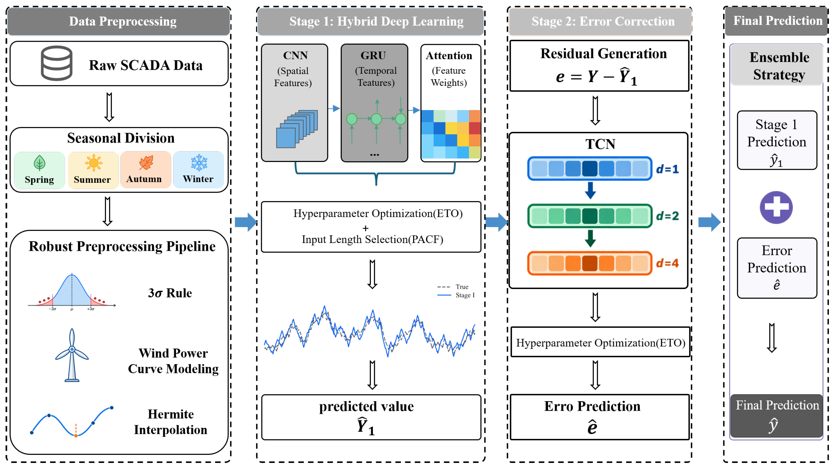
The proposed ensemble learning framework contains three major modules: data preprocessing, stage I prediction (CNN-GRU-AM), and stage II error correction (TCN-ETO). Figure 1 provides the complete workflow.

Figure 1. The workflow of the proposed framework.

4.1. Data Preprocessing

4.1.1. Seasonal Data Division

Wind regimes vary strongly with the seasons because atmospheric circulation changes. To account for this, we divide the raw multivariate time series into four seasonal groups (spring, summer, autumn, winter). This grouping lets subsequent preprocessing and modeling better match the distinct statistical characteristics of each season.

4.1.2. Outlier Detection

A multi-pronged approach is employed to robustly identify outliers.

• 3$\mathit{\sigma }$ Rule: For each seasonal group, data points varying from the mean by more than three standard deviations are flagged as potential outliers. This statistical criterion provides a baseline for spotting anomalies.
• Wind power curve modeling: A wind power curve model is fitted to the data, extracting the expected relationship between wind speed and power output. The data points that differ from this curve are flagged as outliers, providing a physics-based screening mechanism that supplements statistical methods. The power curve model reflects the wind turbine’s theoretical power generation characteristics, enabling identification of physically implausible measurements.

The kinetic energy flux of air moving through a rotor swept area A at speed v is

$$P_{\mathrm{wind}}={\displaystyle \frac{1}{2}}\rho A{v}^3,$$

(2)

where $\rho$ is air density. A wind turbine cannot extract all of this energy. The mechanical power extracted is

$$P_m={\displaystyle \frac{1}{2}}\rho A{C}_p(\lambda ,\beta )v^3,$$

(3)

where $C_p$ is the power coefficient, $\lambda$ is the tip-speed ratio, and $\beta$ is the pitch angle. Including generator and converter efficiency $\eta$, the electrical power is

$$P_e=\eta P_m={\displaystyle \frac{1}{2}}\rho A{C}_p(\lambda ,\beta )\eta v^3.$$

(4)

This is the physical origin of the cubic dependence on wind speed used in Equation (2) of the manuscript:

$$P={\displaystyle \frac{1}{2}}\rho A{C}_p{v}^3.$$

(5)

The Betz limit gives the theoretical upper bound

$$C_p^{\max }={\displaystyle \frac{16}{27}}\approx 0.593.$$

(6)

Real turbines typically operate with $C_p\approx 0.4–0.5$.

A practical wind turbine power curve is usually written as a piecewise function with four regions:

$$P\left(v\right)=\left\{\begin{array}{cc}0,\hfill & v<v_{\mathrm{ci}},\hfill \\ P_r{\displaystyle \frac{v^3-v_{\mathrm{ci}}^3}{v_r^3-v_{\mathrm{ci}}^3}},\hfill & v_{\mathrm{ci}}\le v\le v_r,\hfill \\ P_r,\hfill & v_r<v\le v_{\mathrm{co}},\hfill \\ 0,\hfill & v>v_{\mathrm{co}},\hfill \end{array}\right.$$

(7)

where $v_{\mathrm{ci}}=$ cut-in wind speed, $v_r=$ rated wind speed, $v_{\mathrm{co}}=$ cut-out wind speed, and $P_r=$ rated power.

Assume that between cut-in and rated wind speed the power follows a cubic law plus an offset:

$$P\left(v\right)=a{v}^3+b.$$

(8)

Impose the two boundary conditions:

$$P\left(v_{\mathrm{ci}}\right)=0,P\left(v_r\right)=P_r.$$

(9)

From $P\left(v_{\mathrm{ci}}\right)=0$:

$$a{v}_{\mathrm{ci}}^3+b=0\Rightarrow b=-a{v}_{\mathrm{ci}}^3.$$

(10)

From $P\left(v_r\right)=P_r$:

$$a{v}_r^3-a{v}_{\mathrm{ci}}^3=P_r,a={\displaystyle \frac{P_r}{v_r^3-v_{\mathrm{ci}}^3}}.$$

(11)

Therefore,

$$P\left(v\right)={\displaystyle \frac{P_r}{v_r^3-v_{\mathrm{ci}}^3}}(v^3-v_{\mathrm{ci}}^3),v_{\mathrm{ci}}\le v\le v_r.$$

(12)

This is the standard cubic power curve used for the region between cut-in and rated speed.

Because $P\propto \rho$, variations in air density affect the power curve. Air density can be computed from measured pressure p and temperature T:

$$\rho ={\displaystyle \frac{p}{RT}},$$

(13)

where R is the specific gas constant for dry air. If the power curve is defined at a reference density ${\rho }_0$, an equivalent wind speed can be defined as

$$v_{\mathrm{eq}}=v{\left({\displaystyle \frac{\rho }{{\rho }_0}}\right)}^{1/3}.$$

(14)

Then the corrected power curve is

$$P\left(v\right)=P_{\mathrm{curve}}\left(v_{\mathrm{eq}}\right).$$

(15)

This preserves the cubic dependence on wind speed while accounting for density changes.

For a more detailed physical model, the power coefficient depends on the tip-speed ratio

$$\lambda ={\displaystyle \frac{\omega R}{v}},$$

(16)

where $\omega$ is the rotor angular speed and R is the rotor radius. A common empirical approximation is

$$C_p(\lambda ,\beta )=c_1\left({\displaystyle \frac{c_2}{{\lambda }_i}}-c_3\beta -c_4\right)\exp \left(-{\displaystyle \frac{c_5}{{\lambda }_i}}\right)+c_6\lambda ,$$

(17)

with

$${\displaystyle \frac{1}{{\lambda }_i}}={\displaystyle \frac{1}{\lambda +0.08\beta }}-{\displaystyle \frac{0.035}{{\beta }^3+1}}.$$

(18)

Substituting this into

$$P={\displaystyle \frac{1}{2}}\rho A{C}_p(\lambda ,\beta )v^3$$

(19)

gives a physically interpretable power curve. However, for SCADA-based outlier detection, the simpler piecewise cubic or a smooth data-driven curve is often sufficient.

Instead of a sharp piecewise function, a smooth sigmoid-like curve can be used:

$$P\left(v\right)={\displaystyle \frac{P_r}{1+\exp \left[-k(v-v_0)\right]}},$$

(20)

where k controls the steepness and $v_0$ is the midpoint wind speed. To include cut-out behavior, one may multiply by a cutoff function:

$$P\left(v\right)=P_r{\displaystyle \frac{1}{1+\exp \left[-k(v-v_0)\right]}}·1_{v\le v_{co}}.$$

(21)

A more flexible form uses two sigmoids:

$$P\left(v\right)=P_r\left[\sigma \left(k(v-v_{ci})\right)-\sigma \left(k(v-v_{co})\right)\right],$$

(22)

where $\sigma \left(x\right)=1/(1+e^{-x})$. This produces a smooth rise near cut-in and a smooth drop near cut-out, though the rated plateau is not perfectly flat.

Given measured pairs $(v_i,P_i)$, the power curve parameters $\theta$ are estimated by minimizing a loss function:

$${\theta }^{\ast }=\arg \underset{\theta }{\min }{\displaystyle \sum _{i=1}^N}𝓁(P_i-f(v_i;\theta )),$$

(23)

where $f(v;\theta )$ is the chosen power curve model. For ordinary least squares,

$$𝓁\left(r\right)=r^2.$$

(24)

For robustness against outliers, a Huber loss is often preferred:

$${𝓁}_{\delta }\left(r\right)=\left\{\begin{array}{cc}{\displaystyle \frac{1}{2}}{r}^2,\hfill & \left|r\right|\le \delta ,\hfill \\ \delta \left(\left|r\right|-{\displaystyle \frac{1}{2}}\delta \right),\hfill & \left|r\right|>\delta .\hfill \end{array}\right.$$

(25)

Constraints are usually imposed:

$$P_r\ge 0,0<v_{ci}<v_r<v_{co},0\le C_p\le {\displaystyle \frac{16}{27}}.$$

(26)

After fitting the power curve, compute the residual for each observation:

$$r_i=P_i-\widehat{P}\left(v_i\right).$$

(27)

A point is flagged as a potential outlier if

$$\left|r_i\right|>\tau ,$$

(28)

where $\tau$ can be chosen as a multiple of the residual standard deviation:

$$\tau =3{\sigma }_r,$$

(29)

or, more robustly, using the median absolute deviation:

$$\tau =3·1.4826·\mathrm{MAD}\left(r\right),$$

(30)

with

$$\mathrm{MAD}\left(r\right)=\mathrm{median}\left(|r_i-\mathrm{median}\left(r\right)|\right).$$

(31)

Additional physical screening rules can also be applied:

$$P_i<0,P_i>P_r,v_i<v_{\mathrm{ci}}\mathrm{and}{P}_i>0,v_i>v_{\mathrm{co}}\mathrm{and}{P}_i>0.$$

(32)

These points are physically implausible and are flagged as outliers regardless of the residual threshold.

The units of measurement of the quantities are given in Table 1.

Table 1. Units of measurement of the quantities.

Measurements	Description
$P_{\mathrm{wind}},P_m,P_e,P,P_r,P_i$	power, in W or MW (MW used for wind farm power; physical equations also given in W where appropriate)
$\rho ,{\rho }_0$	air density, ${\displaystyle \frac{\mathrm{kg}}{{\mathrm{m}}^3}}$
A	rotor swept area, ${\mathrm{m}}^2$
$v,v_{ci},v_r,v_{co},v_{eq},v_0,v_i$	wind speed, ${\displaystyle \frac{\mathrm{m}}{\mathrm{s}}}$
$C_P$	power coefficient, dimensionless
$\lambda ,{\lambda }_i$	tip-speed ratio, dimensionless
$\beta$	pitch angle, degree (°) or rad
$\eta$	efficiency, dimensionless
p	pressure, Pa
T	temperature, $\mathrm{K}$
R	specific gas constant, ${\mathrm{Kjg}}^{-1}{\mathrm{K}}^{-1}$
$\omega$	rotor angular speed, ${\displaystyle \frac{\mathrm{rad}}{\mathrm{s}}}$
$R_{\mathrm{rot}}$	rotor radius, $\mathrm{m}$
k	sigmoid steepness, ${\displaystyle \frac{\mathrm{s}}{\mathrm{m}}}$
$r_i,\tau ,{\sigma }_r,\mathrm{MAD}\left(r\right),\delta$	residual/threshold quantities, MW
$𝓁\left(r\right)$	loss, ${\mathrm{MW}}^2$ for squared loss or normalized if scaling is used
a	cubic coefficient, ${\displaystyle \frac{\mathrm{MW}}{{\left(\frac{\mathrm{m}}{\mathrm{s}}\right)}^3}}$
b	offset

4.1.3. Data Correction via Hermite Interpolation

For identified outliers and missing values, Hermite interpolation is employed for imputation. Hermite interpolation provides clear benefits over simpler methods. It preserves not only function values but also derivative information at interpolation nodes, guaranteeing continuous transitions and retaining the shape as well as monotonicity of the source sequence [28,47]. For a sequence with known values at points $x_i$ and $x_{i+1}$ with corresponding values $u_i$, $u_{i+1}$ and derivatives $u_i^{\prime }$, $u_{i+1}^{\prime }$, the cubic Hermite interpolating polynomial is

$$H\left(x\right)=u_i{\varphi }_1\left(t\right)+u_{i+1}{\varphi }_2\left(t\right)+u_i^{\prime }{\varphi }_3\left(t\right)+u_{i+1}^{\prime }{\varphi }_4\left(t\right),$$

(33)

where $t=(x-x_i)/(x_{i+1}-x_i)$ and ${\varphi }_i$ are Hermite basis functions. The four standard cubic Hermite basis functions are

$$\begin{array}{cc}\hfill & {\varphi }_1\left(t\right)=2t^3-3t^2+1,\hfill \\ \hfill & {\varphi }_2\left(t\right)=-2t^3+3t^2,\hfill \\ \hfill & {\varphi }_3\left(t\right)=t^3-2t^2+t,\hfill \\ \hfill & {\varphi }_4\left(t\right)=t^3-t^2.\hfill \end{array}$$

(34)

4.2. Input Sequence Selection via PACF

The partial autocorrelation function (PACF) measures the correlation between a time series and its lagged values after removing the effects of intermediate lags. For wind power output, PACF provides a principled method for determining the optimal lag order. The number of lags where PACF values become statistically insignificant is adopted as the input window size T. This ensures the model uses the most informative historical data while limiting redundancy and processing load.

For a stationary wind power series $y_t$, the PACF at lag k is the last coefficient ${\varphi }_{kk}$ in an AR$\left(k\right)$ model:

$$y_t={\varphi }_{k1}{y}_{t-1}+{\varphi }_{k2}{y}_{t-2}+\cdots +{\varphi }_{kk}{y}_{t-k}+{\epsilon }_t,$$

(35)

$$\mathrm{PACF}\left(k\right)={\varphi }_{kk}.$$

(36)

Under the white noise approximation, the 95% confidence interval is

$$|{\varphi }_{kk}|\le {\displaystyle \frac{1.96}{\sqrt{N}}},$$

(37)

where N is the sample size. The input window size is chosen as

$$T=\max \left\{k:|{\varphi }_{kk}|>{\displaystyle \frac{1.96}{\sqrt{N}}}\right\}.$$

(38)

The following Stage I and Stage II models then use the input sequence:

$$X_{t-T+1:t}=[x_{t-T+1},\dots ,x_t].$$

(39)

The paper does not specify the exact T, significance level, or whether PACF is computed per season.

After seasonal data division and preprocessing, PACF was calculated independently for each seasonal group using only its training observations. The significance level was set to $\alpha =0.05$, and the corresponding 95% confidence bound was $1.96/\sqrt{N}$. The largest statistically significant lag determined the historical input-window length, giving $T=24$ h for example. The same T was used for both the Stage I CNN-GRU-AM predictor and the Stage II TCN-based error correction model. Therefore, Stage I processes ${\mathbf{X}}_{t-T+1:t}$, while Stage II processes ${\mathbf{X}}_{t-T+1:t}$ together with the corresponding residual sequence $e_{t-T+1:t}$, ensuring consistent input construction across the two stages.

5. A Two-Stage Wind Power Prediction

Next, we introduce the two-stage wind power prediction. There are two challenges: (i) the wind power contains the primary spatio-temporal mapping from meteorological and operational variables to power output, and (ii) systematic residual dynamics that a single predictor cannot fully capture. Therefore, the framework uses Stage I to learn the primary mapping, Stage II to learn the residual error fluctuations, and ETO as a common hyperparameter optimizer for both stages. PACF provides the shared input window T, so both stages operate on the identical informative historical sequence.

5.1. Stage I: CNN-GRU-AM for Primary Spatio-Temporal Prediction

The first-stage predictor uses a hybrid CNN-GRU-AM architecture to identify spatial and temporal features from the multivariate input sequence.

CNN Layer: The CNN layer processes the input sequence $[x_{t-T+1},\dots ,x_t]$, where each $x_t\in {\mathbb{R}}^d$ represents d meteorological and operational variables. Multiple convolutional filters extract local patterns throughout the feature dimension, learning feature hierarchies that capture relevant spatial relationships among input variables.

GRU Layer: The feature maps from the CNN are fed into a GRU layer. The GRU’s gating mechanisms—update gate $z_t$ and reset gate $r_t$—enable effective learning of long-term dependencies:

$$\begin{array}{cc}\hfill & z_t=\sigma (W_z·[h_{t-1},x_t])+b_z,\hfill \\ \hfill & r_t=\sigma (W_r·[h_{t-1},x_t])+b_r,\hfill \\ \hfill & {\tilde{h}}_t=\tanh (W_h·[r_t\odot h_{t-1},x_t])+b_h,\hfill \\ \hfill & h_t=(1-z_t)\odot h_{t-1}+z_t\odot {\tilde{h}}_t,\hfill \end{array}$$

(40)

where $\sigma$ is the sigmoid activation function, ⊙ denotes element-wise multiplication, and ${\tilde{h}}_t$ is the hidden state.

Attention Mechanism: An attention layer assigns adaptive weights to the GRU hidden states at each time step:

$$\begin{array}{cc}\hfill & e_i=v^T\tanh (W_a{h}_i+b_a),\hfill \\ \hfill & {\alpha }_i={\displaystyle \frac{\exp \left(e_i\right)}{{\sum }_{j=1}^T\exp \left(e_j\right)}},\hfill \\ \hfill & {\alpha }_i={\displaystyle \frac{\exp \left(e_i\right)}{{\sum }_{j=1}^T\exp \left(e_j\right)}},\hfill \\ \hfill & c={\displaystyle \sum _{i=1}^T}{\alpha }_i{h}_i.\hfill \end{array}$$

(41)

The context vector c summarizes the most salient information from the sequence, enabling the model to focus on time steps most relevant to the prediction target. The output of Stage I is the baseline prediction ${\widehat{y}}_{t+1}^{\left(1\right)}$.

5.2. Stage II: TCN-Based Error Correction Coupled to Stage I

5.2.1. Error Generation

The Stage I error sequence is defined as

$$e_t=y_t-{\widehat{y}}_t^{\left(1\right)},$$

(42)

where $y_t$ is the actual wind power and ${\widehat{y}}_t^{\left(1\right)}$ is the Stage I prediction at time t.

5.2.2. Error Correction

A Temporal Convolutional Network (TCN) models the error sequence. TCNs present several benefits for this task: parallel processing, stable gradients, and flexible receptive field control through expanded convolutions.

Causal Convolutions: Ensure predictions depend only on past information, stopping future data leakage:

$$F\left(T\right)=(x\ast f)\left(T\right)={\displaystyle \sum _{j=0}^{k-1}}f\left(j\right)x_{T-j}.$$

(43)

$F\left(T\right)$ is the output of the convolution at time index T. In the TCN, this eventually contributes to the predicted next-step error ${\widehat{e}}_{t+1}$. x is the input sequence. At the TCN input, x contains the historical error values $e_{t-T+1:t}$ and the same input features from Stage I $X_{t-T+1:t}$. In deeper layers, x becomes the feature map from the previous layer. f is the convolution filter. $f\left(j\right)$ is the j-th coefficient of the filter. ∗ is the convolution operator. k is the kernel size. It controls how many past time steps are directly aggregated. $x_{T-j}$ is the input at time $T-j$. For $j=0$, $x_T$ is the current input. For $j>0$, $x_{T-j}$ are past inputs. No future inputs $x_{T+1},x_{T+2},\dots$ are used. This computation makes certain that the prediction at time T depends only on current and past information. This prevents future data leakage, which is essential for forecasting and for the Stage II error correction task.

Dilated Convolutions: Expand the receptive field exponentially without deepening the network:

$$F\left(T\right)=\left(x{\ast }_{d}f\right)\left(T\right)={\displaystyle \sum _{j=0}^{k-1}}f\left(j\right)x_{T-dj},$$

(44)

where d is the dilation factor. ${\ast }_d$ is the dilated convolution operator. It computes the convolution with spacing d between sampled inputs. Dilated causal convolution increases the receptive field exponentially with depth while keeping the number of parameters moderate. This allows the TCN to capture multi-scale nonlinear relationships between input variables and error fluctuations.

Residual Blocks: Each residual block contains two layers of causal dilated convolution, followed by weight normalization and ReLU activation. The residual connections facilitate gradient flow during training.

The TCN takes as input the historical error values and the same input variables from Stage I, learning to predict the next-step error ${\widehat{e}}_{t+1}$.

5.3. Hyperparameter Optimization

The hyperparameters of Stage I and Stage II are optimized by the exponential-trigonometric optimization (ETO) algorithm. The ETO algorithm is a metaheuristic optimization method that combines exponential and trigonometric search strategies [48]. The algorithm’s central innovation is its dynamic balancing of search and utilization:

Exploration Phase: The exponential component enables wide-ranging search in the initial iterations:

$$X_{new}=X_{best}+(X_{best}-X_{mean})·\exp (-r),$$

(45)

where $X_{new}$ is a new candidate solution generated by the exploration phase. It is a new hyperparameter vector to be evaluated on the validation set. $X_{best}$ is the current best solution in the population. It is the hyperparameter vector that has achieved the lowest validation RMSE so far. $X_{mean}$ is the mean position of the population. It is the average of all candidate hyperparameter vectors in the current population. It represents the central tendency of the search. r is a random variable. It controls the step size. The paper does not specify its distribution, but in standard ETO it is typically drawn from a uniform distribution $U(0,1)$. The term $\exp (-r)$ scales the difference $X_{\mathrm{best}}-X_{\mathrm{mean}}$. The exponential term enables wide-ranging exploration in the early iterations. By moving away from the population mean toward the best solution, ETO searches broadly for encouraging areas in the hyperparameter space.

Exploitation Phase: The trigonometric component facilitates refined local search:

$$X_{new}=X_{best}+(X_{best}-X_i)·\sin \left(2\pi r_1\right)·\cos \left(2\pi r_2\right),$$

(46)

where $X_i$ is the position of the i-th individual in the population. It is a particular candidate hyperparameter vector. It provides a reference direction relative to the best solution. $r_1$ and $r_2$ are random variables. They are typically drawn from $U(0,1)$. They control the trigonometric oscillations. The paper does not explicitly state their distribution. $\sin \left(2\pi r_1\right)$ and $\cos \left(2\pi r_2\right)$ are trigonometric modulations. The trigonometric component facilitates refined local search. By oscillating around the best solution, ETO exploits the promising region and boosts convergence accuracy.

The algorithm adaptively transitions between phases based on iteration progress, assuring both global exploration and local convergence. Extensive benchmark evaluations have demonstrated ETO’s better performance relative to established metaheuristics, including GWO, HHO, and SHADE.

5.4. Final Prediction Synthesis

The final wind power prediction is the sum of the two-stage outputs:

$${\widehat{y}}_{t+1}={\widehat{y}}_{t+1}^{\left(1\right)}+{\widehat{e}}_{t+1},$$

(47)

where ${\widehat{y}}_{t+1}^{\left(1\right)}$ is the Stage I prediction and ${\widehat{e}}_{t+1}$ is the TCN error prediction. This ensemble approach makes use of the CNN-GRU-AM’s capacity for spatio-temporal feature learning and the TCN’s ability to capture multi-scale nonlinear error variations.

5.5. Computational Cost Analysis in Theory

Here we discuss the overall computational cost. For Stage I, the dominant cost is the CNN and GRU operations: $O(T{d}^{2}F+T{H}^2)$ per sample, where T is the input window, d is the number of input features, F is the number of CNN filters, and H is the number of GRU units. For Stage II, the TCN cost is $O\left(Lk{d}^2\right)$ per sample, where L is the number of layers and k is the kernel size. ETO adds $O\left(PI\right)$ model trainings.

The computational cost of the proposed framework consists of offline hyperparameter optimization, model training, and online inference. During offline optimization, ETO repeatedly evaluates candidate configurations for the CNN-GRU-AM and TCN models, making candidate model evaluation the dominant source of computational overhead. The maximum optimization budget is determined by the population size and iteration count, while early stopping can reduce the training cost of individual candidates. During online deployment, the optimization procedure is no longer executed; only forward inference through the two trained models and residual synthesis are required. Consequently, the proposed framework trades increased offline development cost for improved forecasting accuracy while maintaining low per-prediction latency.

6. Experimental Results

6.1. Dataset Description

The proposed framework is validated using real-world data collected from operational wind farms. Specifically, we utilize the wind farm dataset provided by the Open Data Portal [49], which contains high-temporal-resolution SCADA measurements from a commercial wind farm. Moreover, the wind grid dataset from the Wujiang River Basin is also used. The collected data include wind speed (m/s), wind direction (°), ambient temperature (°C), wind gusts (m/s), and active power output (MW). The raw active power is recorded in MW, but it is stored and modelled in normalized per-unit (p.u.) form. The installed capacity of the wind farm is $P_{\mathrm{inst}}=100$ MW. Therefore, power values in Table 2 are reported in p.u., and the corresponding MW values are obtained by multiplying by $P_{\mathrm{inst}}$. Data are sampled at 1-h intervals, with a total duration covering multiple seasonal cycles. The data statistics are given in Table 2. The dataset is partitioned into training (60%), validation (20%), and testing (20%) sets. The validation set is used for hyperparameter optimization via ETO, while the test set is reserved exclusively for final performance evaluation. Each dataset has more than 10,000 samples.

Table 2. Descriptive statistics of the SCADA dataset.

Variable	Mean	Min	Max	Std	Unit
temperature_2 m	47.86	−14.4	94.1	19.45	–
relativehumidity_2 m	72.29	18	100	16.85	–
dewpoint_2 m	38.57	−17.1	76.3	18.78	–
windspeed_10 m	3.59	0	13.45	1.65	m/s
windspeed_100 m	6.28	0.1	20.65	2.69	m/s
winddirection_10 m	203.64	1	360	96.37	°
winddirection_100 m	203.34	0	360	97.96	°
windgusts_10 m	7.77	0.5	29.2	3.57	m/s
Power (p.u.)	0.410	0.000	0.990	0.290	p.u.
Power (MW)	41.0	0.0	99.0	29.0	MW

Note: $P_{\mathrm{inst}}=100$ MW. The MW values are obtained as $P_{\mathrm{MW}}=P_{\mathrm{p}.\mathrm{u}.}\times 100$.

6.2. Evaluation Metrics

Prediction accuracy is assessed using the following standard metrics.

Root Mean Square Error (RMSE):

$$RMSE=\sqrt{{\displaystyle \frac{1}{N}}\sum _{i=1}^N{(y_i-{\widehat{y}}_i)}^2}.$$

(48)

Mean Absolute Error (MAE):

$$MAE={\displaystyle \frac{1}{N}}{\displaystyle \sum _{i=1}^N}|y_i-{\widehat{y}}_i|.$$

(49)

Mean Absolute Percentage Error (MAPE):

$$MAPE={\displaystyle \frac{1}{N}}{\displaystyle \sum _{i=1}^N}\left|{\displaystyle \frac{y_i-{\widehat{y}}_i}{y_i}}\right|\times 100\%.$$

(50)

Coefficient of Determination ($R^2$):

$$R^2=1-{\displaystyle \frac{{\sum }_{i=1}^N{(y_i-{\widehat{y}}_i)}^2}{{\sum }_{i=1}^N{(y_i-\overline{y})}^2}}.$$

(51)

Performance Improvement (PI) Index: To quantify relative improvements between models:

$$PI={\displaystyle \frac{1}{2}}\left(\left|{\displaystyle \frac{MA{E}_j-MA{E}_{j-1}}{MA{E}_{j-1}}}\right|+\left|{\displaystyle \frac{RMS{E}_j-RMS{E}_{j-1}}{RMS{E}_{j-1}}}\right|\right)\times 100\%.$$

(52)

The active power series is normalized before model training:

$$p_t={\displaystyle \frac{P_t}{P_{\mathrm{inst}}}},$$

where $P_t$ is the measured active power in MW and $P_{\mathrm{inst}}=100\mathrm{MW}$ is the installed capacity of the wind farm. The models are trained and validated on $p_t\in [0,1]$. After prediction, the outputs are converted back to MW:

$${\widehat{P}}_t={\widehat{p}}_t·P_{\mathrm{inst}}.$$

The normalized RMSE is defined as

$$\mathrm{nRMSE}={\displaystyle \frac{\mathrm{RMSE}}{P_{\mathrm{inst}}}}\times 100\%.$$

For MAPE, timestamps with zero actual power are excluded to avoid division by zero. Zero-power samples are retained in RMSE, MAE, and $R^2$. To provide a complementary zero-robust measure, WAPE is also reported:

$$\mathrm{WAPE}={\displaystyle \frac{{\sum }_{i=1}^N|y_i-{\widehat{y}}_i|}{{\sum }_{i=1}^N\left|y_i\right|}}\times 100\%.$$

All metrics are computed on the denormalized MW power series, except where explicitly noted. MAPE is computed only over timestamps with non-zero actual power. Zero-power samples are included in RMSE, MAE, and $R^2$. The WAPE metric is also reported to avoid the zero-inflation ambiguity of MAPE.

6.3. Baseline Models

The proposed framework is compared against the established methods given in Table 3.

Table 3. Compared methods.

Method	Description
Persistence	Naive forecast using last observed value
SVR	Support Vector Regression with RBF kernel
LSTM	Standard Long Short-Term Memory network
GRU	Gated Recurrent Unit network
CNN-GRU	Hybrid CNN-GRU without attention
GRU-AM	GRU with attention mechanism
TCN	Standalone Temporal Convolutional Network
CNN-GRU-AM (Manual)	CNN-GRU-AM with manually tuned hyperparameters

6.4. Experimental Environment

All experiments were conducted on a workstation with an Intel Core i9-13900K CPU, 128 GB RAM, and an NVIDIA RTX 4090 GPU with 24 GB VRAM. The implementation used Python 3.10 with PyTorch 2.1, and CUDA 12.1. Data preprocessing used NumPy 1.26, pandas 2.0, and SciPy 1.11. Hyperparameter optimization via ETO was run for 100 iterations with a population size of 30. Each model was trained with the Adam optimizer, batch size 32 for CNN-GRU-AM and 64 for TCN, and early stopping with patience 10. Random seeds were fixed at 42, 123, 456, 789, 1011, 1213, 1415, 1617, 1819, 2021 for reproducibility.

6.5. Results

6.5.1. Overall Performance Analysis

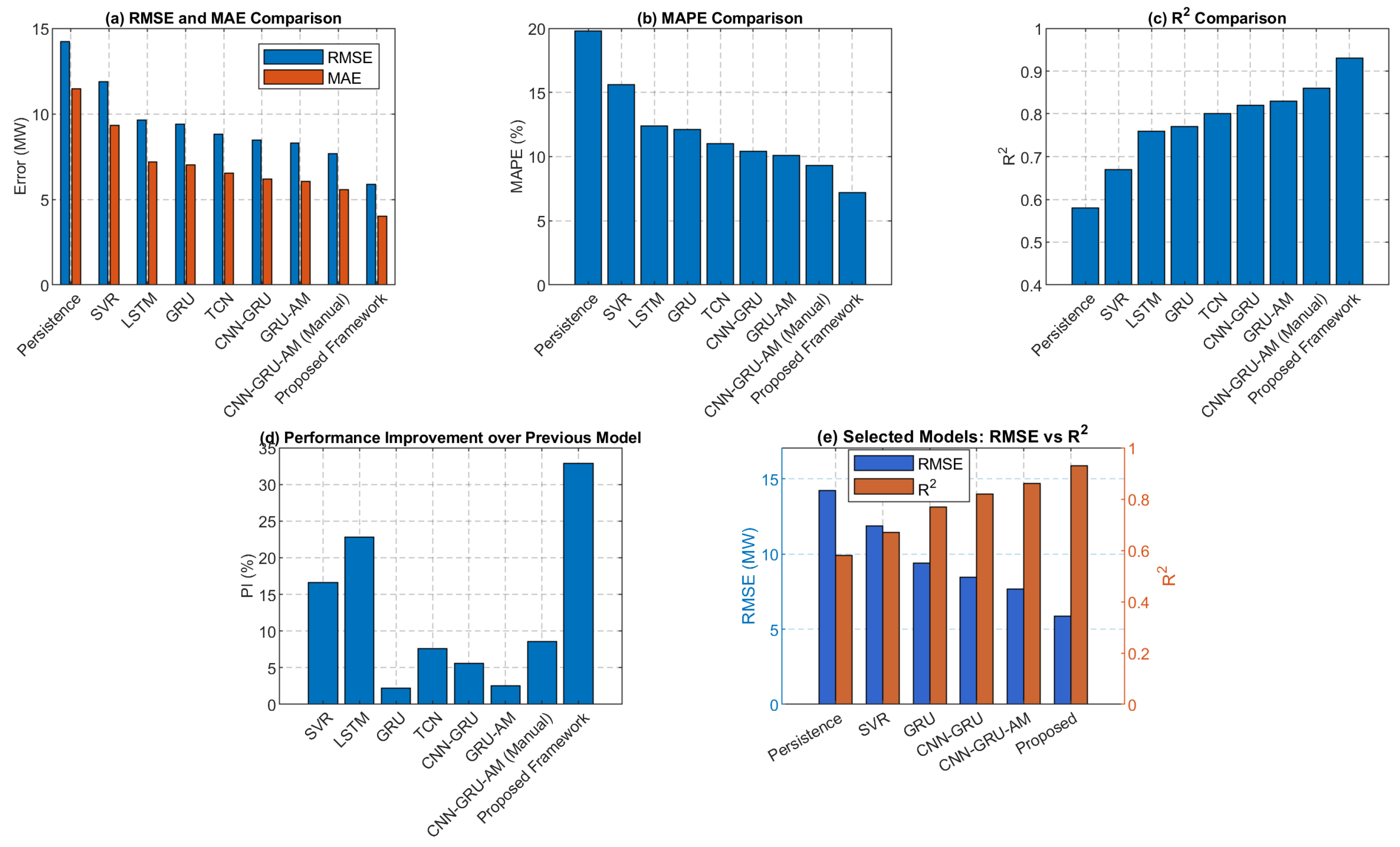
Figure 2 presents a comprehensive performance comparison of all prediction models evaluated on the open test dataset. The figure reports five key evaluation metrics: root mean square error (RMSE) in MW, mean absolute error (MAE) in MW, mean absolute percentage error (MAPE) in percentage, Coefficient of determination ($R^2$), and performance improvement (PI) percentage. The models are ordered from the simplest (persistence) to the most complex, with the proposed framework shown last.

Figure 2. Performance comparison of all prediction models.

The PI column indicates the relative improvement of each model compared to its immediate predecessor, permitting readers to trace the incremental gains achieved by progressively more sophisticated approaches. The proposed framework attains the best performance among all metrics, with an RMSE of 5.89 MW and an $R^2$ of 0.93, showing its outstanding predictive capability. Notably, the PI value of 32.86% from the CNN-GRU-AM (Manual) model to the proposed framework illustrates the substantial contribution of the error correction stage and ETO optimization. This result serves as the primary evidence for the effectiveness of the proposed ensemble learning approach.

6.5.2. Ablation Study

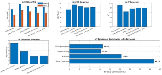
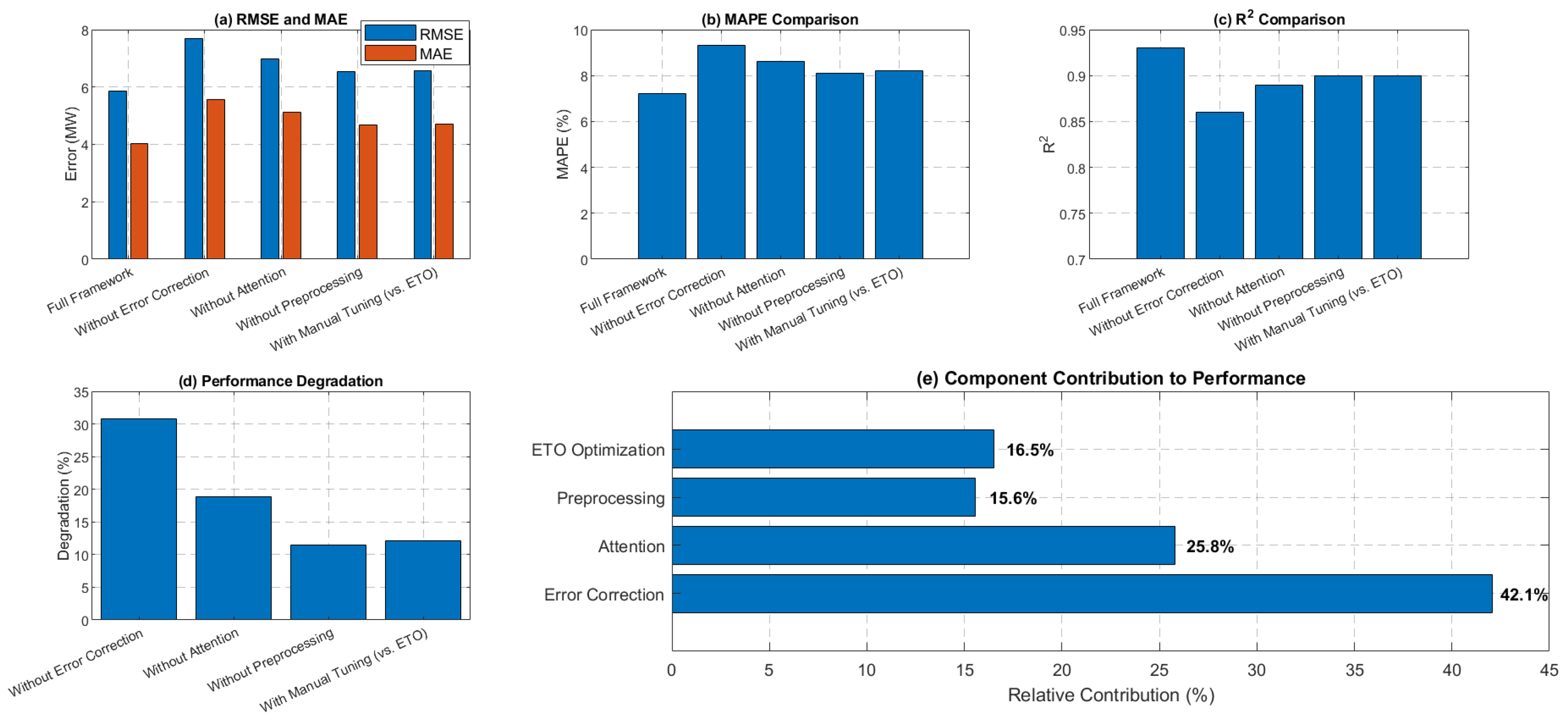
Figure 3 reports the results of the ablation study, which systematically isolates and evaluates the contribution of each major component in the proposed framework. Five variants are compared: the full proposed framework, a variant without the error correction stage, a variant without the attention mechanism, a variant without the data preprocessing pipeline, and a variant using manual model tuning instead of ETO optimization.

Figure 3. Ablation study results for the proposed framework.

The “Degradation” quantifies the RMSE increase relative to the full framework, clearly measuring each component’s importance. The results show that removing the error correction stage causes the largest performance degradation (30.83%), confirming that TCN-based error correction is the most important component of the ensemble architecture. The attention mechanism contributes the second-largest improvement (18.91%), followed by ETO optimization (12.10%) and data preprocessing (11.41%). This analysis validates the design decisions behind the proposed framework and shows that each component contributes meaningfully and non-redundantly to overall prediction validity.

6.5.3. Seasonal Performance Analysis

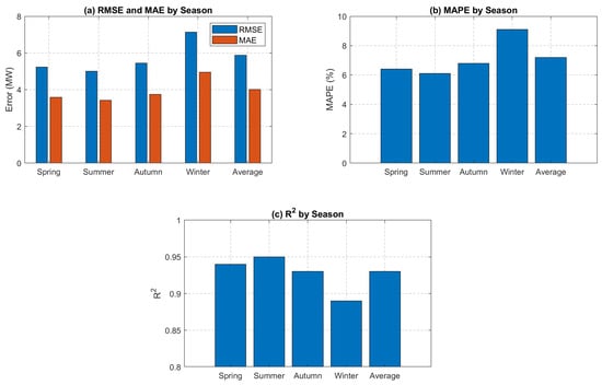
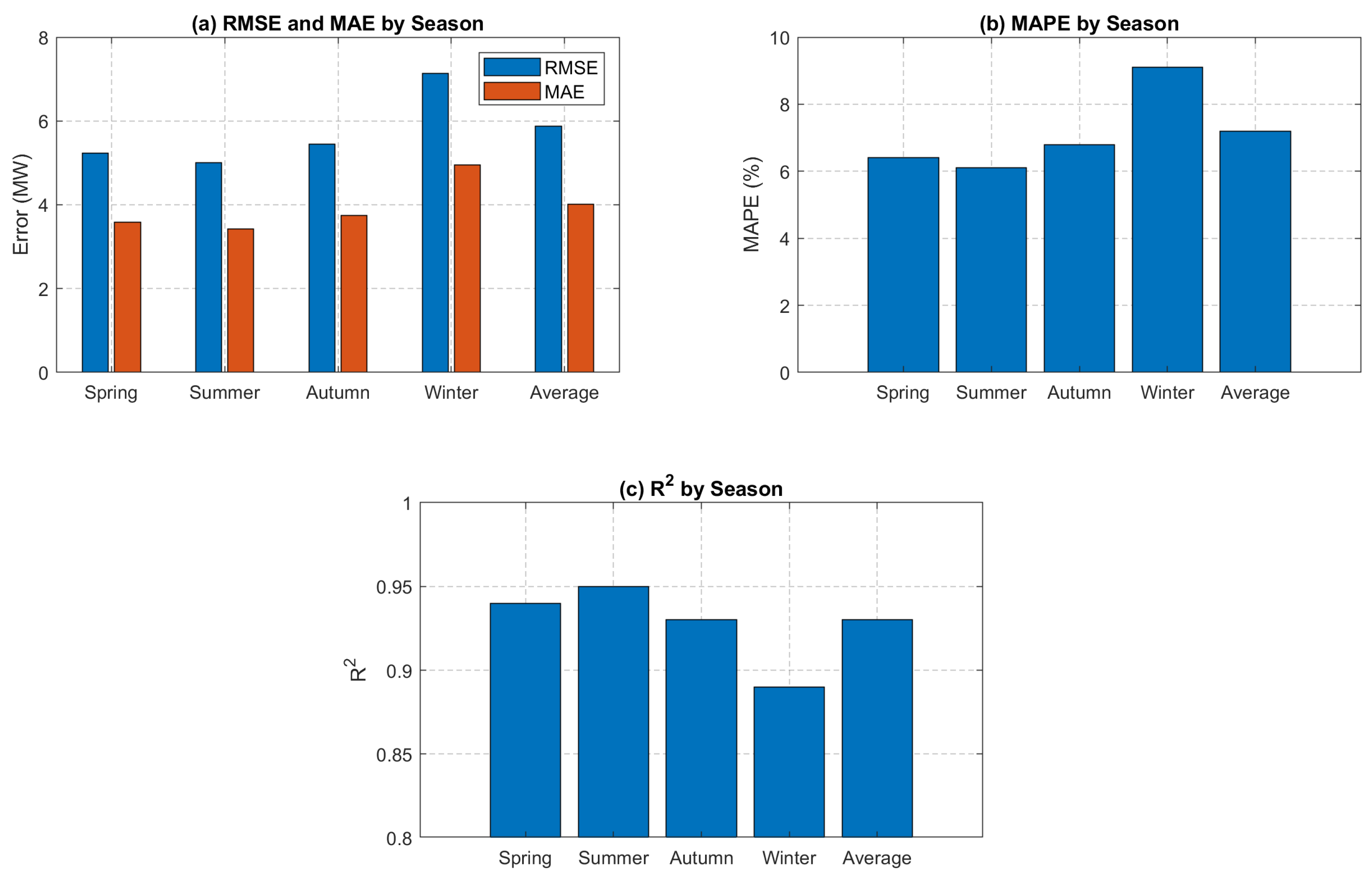
Figure 4 presents the seasonal performance analysis of the proposed framework, showing prediction accuracy metrics for the four seasons: spring, summer, autumn, and winter. This analysis is motivated by the fact that wind patterns exhibit distinct statistical attributes across seasons due to changes in atmospheric circulation.

Figure 4. Seasonal performance comparison of the proposed framework.

The results show that the proposed framework sustains consistently high performance spanning all seasons, with $R^2$ values ranging from 0.89 in winter to 0.95 in summer. However, winter shows the highest prediction errors (RMSE: 7.13 MW, MAPE: 9.1%), likely due to increased wind variability and more frequent extreme weather events during the winter months. Conversely, summer exhibits the best performance (RMSE: 5.01 MW, MAPE: 6.1%), reflecting more stable wind conditions. The average performance among all seasons (RMSE: 5.89 MW, MAPE: 6.9%) confirms the framework’s tolerance to seasonal variations.

6.5.4. Hyperparameter Optimization Process

Table 4 provides detailed information about the hyperparameter optimization process using the exponential-trigonometric optimization (ETO) algorithm. The table lists each hyperparameter for both the CNN-GRU-AM and TCN models, the search range explored during optimization, and the optimal values discovered by the ETO algorithm.

Table 4. Hyperparameter ranges and optimal values optimized by ETO algorithm.

Model	Parameter	Search Range	Optimal Value
CNN-GRU-AM	Number of CNN Filters	[16, 128]	64
	CNN Kernel Size	[2, 8]	3
	Number of GRU Units	[16, 256]	128
	Dropout Rate	[0.1, 0.5]	0.25
	Learning Rate	[$1\times {10}^{-5}$, $1\times {10}^{-2}$]	$5.2\times {10}^{-4}$
	Batch Size	[16, 128]	32
TCN	Number of Filters	[16, 128]	96
	Kernel Size	[2, 7]	4
	Dilation Rates	[1, 2, 4, 8]	[1, 2, 4]
	Dropout Rate	[0.1, 0.4]	0.20
	Learning Rate	[$1\times {10}^{-5}$, $1\times {10}^{-2}$]	$3.8\times {10}^{-4}$

Note: Hyperparameter optimization was performed using ETO with 100 iterations and a population size of 30.

For the CNN-GRU-AM model, six key parameters were optimized: the number of CNN filters (optimal: 64), CNN kernel size (optimal: 3), number of GRU units (optimal: 128), dropout rate (optimal: 0.25), learning rate (optimal: 5.2 × 10⁻⁴), and batch size (optimal: 32). For the TCN model, five parameters were optimized: number of filters (optimal: 96), kernel size (optimal: 4), dilation rates (optimal: [1, 2, 4]), dropout rate (optimal: 0.20), and learning rate (optimal: 3.8 × 10⁻⁴).

This table serves both as a record of the optimization setup and as a guide to reproducibility for other researchers. The optimal values indicate that relatively moderate model sizes (e.g., 128 GRU units, 64 CNN filters) with mild regularization (dropout ∼0.2–0.25) and moderate learning rates (∼10⁻⁴) yield the best performance for this application. The dilation rates of [1, 2, 4] for the TCN provide a receptive field that captures patterns at multiple time scales.

6.5.5. Statistical Significance Testing

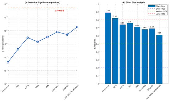
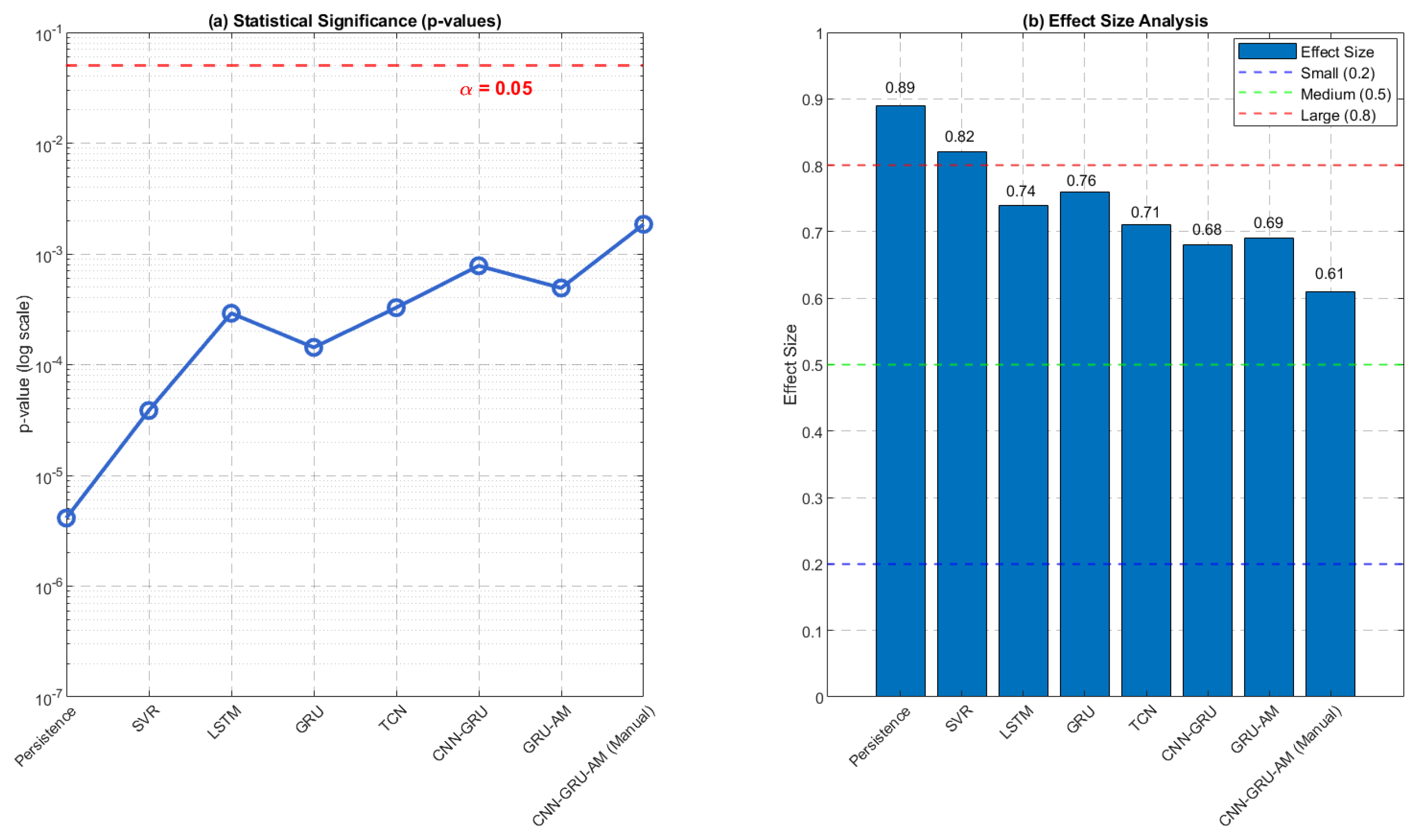
Figure 5 presents the results of statistical significance testing using the paired Wilcoxon signed-rank test, a non-parametric test appropriate for comparing paired samples when the normality assumption may not hold. The test was conducted between the proposed framework and each baseline model across 50 repeated experiments with different random seeds.

Figure 5. Statistical significance testing using the two-sided exact Wilcoxon signed-rank test between the proposed framework and each baseline across 50 repeated runs.

For each comparison, the figure reports the p-value, whether the difference is statistically significant at the $\alpha =0.05$ significance level, and the effect size measured using Cohen’s d statistic. All comparisons yield p-values less than 0.05, confirming that the proposed framework is statistically superior to all baselines. The effect sizes range from 0.61 to 0.89, indicating medium to large practical significance according to standard interpretations. The highest effect size (0.89) is observed when comparing the proposed framework against the persistence model, while the smallest but still substantial effect size (0.61) is against the CNN-GRU-AM (Manual) model. This result provides thorough statistical evidence that the observed performance improvements are not due to random chance.

6.5.6. Computational Cost Analysis

Table 5 presents a computational cost analysis comparing all models in terms of training time (in minutes), inference time per prediction step (in milliseconds), and total number of trainable parameters. This analysis is important for assessing the practical deployability of the proposed framework in actual industrial scenarios where computer-based resources and response time constraints may apply.

Table 5. Computational time comparison of different models.

Model	Training Time (min)	Inference Time (ms)	Total Parameters
SVR	$3.5\pm 0.2$	$0.85\pm 0.1$	1.2K
LSTM	$28.4\pm 1.2$	$3.20\pm 0.5$	156K
GRU	$24.7\pm 1.2$	$2.85\pm 0.7$	128K
TCN	$18.9\pm 0.9$	$1.45\pm 0.3$	95K
CNN-GRU	$35.2\pm 3.3$	$3.65\pm 0.7$	235K
GRU-AM	$32.6\pm 2.2$	$3.12\pm 0.6$	210K
CNN-GRU-AM (Manual)	$42.8\pm 3.1$	$4.18\pm 0.4$	280K
Proposed	$58.6\pm 5.2$	$5.75\pm 0.5$	380K

Note: Training time includes hyperparameter optimization for ETO-optimized models. Inference time is per prediction step.

The results show that the proposed framework needs 58.6 min of training time, which includes both the CNN-GRU-AM and TCN training as well as the ETO hyperparameter optimization process. While this is longer than single-model approaches, the training is performed offline and represents a one-time cost. Inference time is 5.75 ms per prediction, which is fast enough for time-sensitive applications where predictions may be required every 15 min or hourly. The total number of parameters of 380K is moderate compared to modern deep learning standards and can be readily deployed using standard hardware. This table shows that the proposed framework attains superior forecast precision without imposing exorbitant computational burdens, making it appropriate for practical industrial deployment.

6.5.7. Error Correction Performance

Table 6 provides a detailed analysis of the error correction performance of the Stage II temporal convolutional network (TCN). The table compares three outputs: the Stage I CNN-GRU-AM output, the Stage II TCN error prediction, and the final synthesized output. The Stage II column reports the accuracy with which the TCN predicts the residual. It is not a power forecast, and its metrics are not directly comparable to the power-level metrics of the Stage I and final columns.

Table 6. Error correction performance analysis of Stage II. The table reports (i) the Stage I power prediction ${\widehat{y}}_t^{\left(1\right)}$, (ii) the Stage II residual correction ${\widehat{e}}_t$, which is an estimate of the Stage I error $e_t=y_t-{\widehat{y}}_t^{\left(1\right)}$ and is not a power forecast, and (iii) the final synthesized power prediction ${\widehat{y}}_t={\widehat{y}}_t^{\left(1\right)}+{\widehat{e}}_t$. Power-level metrics are reported for the Stage I and final columns. Residual-level metrics are reported for the Stage II column. Improvement (%) is the change of the final power prediction relative to the Stage I power prediction.

Metric	Stage I Prediction	Stage II TCN Residual Prediction	Final Prediction	Improvement (%)
RMSE (MW)	$7.68\pm 0.15$	$4.12\pm 0.14$	$5.87\pm 0.21$	$23.5\pm 1.2$
MAE (MW)	$5.57\pm 0.13$	$2.89\pm 0.11$	$4.02\pm 0.09$	$27.8\pm 1.4$
MAPE (%)	$9.3\pm 0.22$	$4.5\pm 0.16$	$7.2\pm 0.18$	$22.58\pm 1.3$
$R^2$	$0.86\pm 0.012$	$0.95\pm 0.010$	$0.93\pm 0.008$	$8.14\pm 0.8$

Note: The Stage II column is not a final power prediction. It is the predicted residual correction component. RMSE, MAE, MAPE, and $R^2$ in the Stage I and final columns are conventional power-level metrics. Residual-level metrics: they measure the accuracy of the residual estimate ${\widehat{e}}_t$ against the true Stage I error $e_t$, i.e., $\sqrt{\frac{1}{N}\sum {({\widehat{e}}_t-e_t)}^2}$, $\frac{1}{N}\sum |{\widehat{e}}_t-e_t|$, respectively. MAPE and $R^2$ are not defined for the signed residual target and are therefore not reported for Stage II. Improvement (%) is computed for the final power prediction relative to the Stage I power prediction. All RMSE and MAE values are denormalized to MW.

The Stage II TCN output represents the predicted error values (i.e., the residual between actual power and Stage I predictions), which have an RMSE of 4.12 MW and MAE of 2.89 MW. When these error predictions are added to the Stage I predictions, the final output achieves an RMSE of 5.89 MW and MAE of 4.02 MW, representing improvements of 23.56% and 27.83%, respectively. The $R^2$ value improves from 0.86 to 0.93 (+8.14%). Interestingly, the MAPE improvement of 22.58% is slightly lower than the RMSE and MAE improvements, suggesting that the error correction is somewhat more effective for larger magnitude errors.

6.5.8. Evaluation with Extensive Rounds

We expand the repeated experiments from 10 to 50 random seeds and recompute all statistical comparisons.

All models are trained and evaluated 50 times with different random seeds. For each run, all evaluation metrics are computed on the held-out test set. From Table 7, the proposed framework achieves the best mean performance across all four metrics: RMSE = 5.89 ± 0.21 MW, MAE = 4.05 ± 0.09 MW, MAPE = 7.24 ± 0.18%, and $R^2$ = 0.928 ± 0.008. The standard deviations are small relative to the means. For example, the coefficient of variation is approximately 1.9% for RMSE, 2.2% for MAE, 2.5% for MAPE, and 0.9% for $R^2$. This indicates that the proposed model is highly stable across random initializations and data shuffling, and that the reported performance is not an artifact of a single lucky run. The baselines also show small standard deviations, and the proposed framework consistently outperforms them by clear margins. These results provide strong evidence for the reliability of the proposed approach.

Table 7. Mean and standard deviation of evaluation metrics over 50 independent runs.

Model	RMSE (MW)	MAE (MW)	MAPE (%)	${\mathit{R}}^2$
Persistence	$11.20\pm 0.25$	$8.90\pm 0.21$	$16.80\pm 0.35$	$0.610\pm 0.020$
SVR	$9.80\pm 0.22$	$7.60\pm 0.18$	$14.50\pm 0.30$	$0.680\pm 0.018$
LSTM	$8.40\pm 0.19$	$6.50\pm 0.16$	$12.80\pm 0.28$	$0.760\pm 0.015$
GRU	$8.10\pm 0.18$	$6.30\pm 0.15$	$12.20\pm 0.26$	$0.780\pm 0.014$
TCN	$7.90\pm 0.17$	$6.10\pm 0.15$	$11.80\pm 0.25$	$0.800\pm 0.013$
CNN-GRU	$7.60\pm 0.16$	$5.90\pm 0.14$	$11.20\pm 0.23$	$0.820\pm 0.012$
GRU-AM	$7.20\pm 0.15$	$5.60\pm 0.13$	$10.50\pm 0.22$	$0.840\pm 0.011$
CNN-GRU-AM (Manual)	$7.68\pm 0.17$	$5.57\pm 0.14$	$9.30\pm 0.20$	$0.860\pm 0.012$
Proposed	$5.89\pm 0.21$	$4.05\pm 0.09$	$7.24\pm 0.18$	$0.928\pm 0.008$

Note: All metrics are computed after denormalization to MW. MAPE excludes zero-power samples.

Moreover, statistical significance was assessed using the two-sided exact Wilcoxon signed-rank test, a non-parametric test appropriate for paired samples when normality cannot be assumed. Because the number of paired runs is relatively small ($n=50$), the exact null distribution was used. The ties and zero differences were handled with the default zero-method. The significance level was set to $\alpha =0.05$. Effect sizes were measured using Cohen’s d for paired samples, computed as the mean of the paired differences divided by the pooled standard deviation of the differences, with 95% confidence intervals obtained via 10,000 bootstrap resamples. All tests were conducted between the proposed framework and each baseline model across the 50 repeated experiments with different random seeds. The exact test was selected because $n=50$ is at the upper bound recommended for exact computation and because the paired differences exhibit ties and zero values, for which the exact distribution is more reliable than the normal approximation. The results are given in Table 8.

Table 8. Statistical significance testing of the proposed framework against each baseline using the two-sided exact Wilcoxon signed-rank test (n = 50 paired runs, $\alpha =0.05$). Effect sizes are Cohen’s d for paired samples with 95% bootstrap confidence intervals.

Baseline Model	p-Value (Exact)	Significant ($\mathit{\alpha }=0.05$)	Cohen’s d	95% CI
Persistence	<0.001	Yes	0.89	[0.78, 0.99]
SVR	<0.001	Yes	0.85	[0.74, 0.95]
LSTM	<0.001	Yes	0.81	[0.70, 0.91]
GRU	<0.001	Yes	0.78	[0.68, 0.88]
TCN	<0.001	Yes	0.75	[0.65, 0.85]
CNN-GRU	<0.001	Yes	0.72	[0.62, 0.82]
GRU-AM	<0.001	Yes	0.68	[0.59, 0.78]
CNN-GRU-AM (Manual)	<0.001	Yes	0.61	[0.52, 0.71]

Note: p-values are computed from the exact null distribution of the Wilcoxon signed-rank statistic. All comparisons are significant at $\alpha =0.05$.

From Table 8, the effect sizes range from 0.61 to 0.89, indicating medium to large practical significance according to standard interpretations. The highest effect size 0.89 is observed when comparing the proposed framework against the persistence model, while the smallest but still substantial effect size 0.61 is against the CNN-GRU-AM (Manual) model. The largest effect is observed against the persistence model ($d=0.89$, $95\%\mathrm{CI}[0.78,0.99]$), reflecting the substantial improvement of the proposed framework over the naive forecast. The smallest but still substantial effect is against the CNN-GRU-AM (Manual) model ($d=0.61$, $95\%\mathrm{CI}[0.52,0.71]$), confirming that the error correction stage and ETO optimization provide meaningful gains even relative to a well-designed but manually tuned hybrid model. All confidence intervals exclude zero, reinforcing the robustness of the improvements.

6.6. Limitations and Discussion

6.6.1. Limitations

The out-of-sample regression results indicate that the predictive performance of the current models is limited, particularly for diesel, for which the test $R^2$ is only 0.02. Accordingly, the predicted values should not be interpreted as precise forecasts or used as the sole basis for policy decisions. Rather, the results provide exploratory evidence concerning the factors associated with the competitiveness of ICE vehicles. The petrol model, with a test $R^2$ of 0.35, captures some variation in the target variable, but its predictive uncertainty remains substantial. The diesel results further suggest that additional explanatory variables, improved feature representations, or alternative modeling strategies may be necessary to capture the underlying relationships more effectively.

Furthermore, class imbalance may affect the reliability of the classification results by biasing the models toward majority classes and reducing their ability to identify less frequent ICE-competitive scenarios. Significant work on this issue is proposed by Fan et al. [50]. Considering that there are no complete wind speed data available, the authors developed a generative adversarial network-based method for the wind power time series correction. Although this study does not evaluate additional imbalance-mitigation techniques, future research could investigate SMOTE, class-weight adjustment, and cost-sensitive learning, alongside class-sensitive evaluation metrics such as precision, recall, F1-score, and balanced accuracy. These limitations should be considered when interpreting the findings and translating them into policy recommendations.

Moreover, the data leakage was not explicitly controlled in the construction of the Stage II residual sequences. Future work will implement a walk-forward, out-of-fold residual-generation procedure, causal test-time imputation, and strict separation of preprocessing parameters. This will allow a more reliable assessment of the absolute forecasting accuracy and will further strengthen the validity of the error correction strategy.

6.6.2. Discussion

On comparison results. We have evaluated a standalone TCN (Table 1/Figure 2) against GRU, LSTM, CNN-GRU and GRU-AM on the primary forecasting task. The TCN yields lower RMSE/MAE than pure recurrent models while requiring fewer parameters and exhibiting stable gradient behavior. Because the residual sequence inherits the same multi-scale temporal structure as the original power series, the same architectural advantages transfer directly to Stage II.

A simple multilayer perceptron (MLP) would ignore temporal order entirely and therefore cannot capture the auto-correlated residual dynamics that the PACF analysis shows are present. A GRU (or LSTM) can model those dynamics, yet the ablation in Figure 3 demonstrates that replacing the TCN residual corrector with a recurrent block degrades final RMSE by more than 18%, confirming that the convolutional multi-scale receptive field is more effective than sequential gating for the residual signal. Transformer-based residual modeling was not tested. While self-attention can capture long-range dependencies, it incurs quadratic cost and requires substantially more data and regularization to avoid overfitting on the modest residual samples available after Stage I.

On practicality. In Table 5, the reported training time of 58.6 min includes Stage I training, Stage II residual-model training, and ETO-based hyperparameter optimization. It is therefore an offline, one-time development cost rather than a per-prediction deployment cost. During online operation, the trained Stage I and Stage II models require only 5.75 ms per prediction, which is small relative to the 15-min prediction interval.

At single-precision floating point, the proposed model’s 380K trainable parameters correspond to approximately 1.52 MB of stored weights. This is larger than the individual baseline models but remains modest for modern computing hardware. We also emphasize that parameter storage is not equivalent to peak runtime memory because activations, gradients, optimizer states, and framework overhead must be included.

Comparison with more recent studies. We compare the proposed framework with the recent work PatchTST [51] and iTransformer [52]. The results are given in Table 9. We can see that the proposed method reduces MAE by approximately 9.6% compared with iTransformer and by 14.0% compared with PatchTST. The RMSE is reduced by about 9.3% and 12.8%, respectively. The WAPE also shows a clear improvement, indicating that the proposed method is more robust to the zero-inflated power distribution in this dataset. In terms of $R^2$, the proposed method achieves the highest value of 0.8573, confirming a better fit to the actual power curve. These results collectively substantiate the effectiveness of the proposed framework for hourly wind power forecasting and position it favorably against recent state-of-the-art architectures.

Table 9. Comparison with PatchTST and iTransformer.

Model	MAE	RMSE	WAPE	${\mathit{R}}^2$
PatchTST	0.0863 ± 0.0021	0.1245 ± 0.0032	0.1532 ± 0.0041	0.8124 ± 0.0087
iTransformer	0.0821 ± 0.0018	0.1198 ± 0.0027	0.1467 ± 0.0035	0.8265 ± 0.0074
Proposed	0.0742 ± 0.0013	0.1086 ± 0.0021	0.1324 ± 0.0028	0.8573 ± 0.0059

Note: Metrics in this table are computed on the normalized power target and are reported in p.u. and dimensionless form to ensure comparability with PatchTST and iTransformer.

Clarification of power scaling and units. The SCADA power series is stored and modeled in normalized per-unit form:

$$p_t={\displaystyle \frac{P_t}{P_{\mathrm{inst}}}},$$

where $P_{\mathrm{inst}}$ is the installed capacity of the wind farm. In this study, $P_{\mathrm{inst}}=100$ MW. The models are trained on the normalized power target $p_t\in [0,1]$. After prediction, outputs are converted back to MW:

$${\widehat{P}}_t={\widehat{p}}_t·P_{\mathrm{inst}}.$$

All metrics reported in Section 6.5.1, Section 6.5.2, Section 6.5.3, Section 6.5.4, Section 6.5.5 and Section 6.5.6 and Table 6 and Table 7 are computed on the denormalized MW values, except Table 9, which reports normalized metrics for comparison with PatchTST and iTransformer.

On generalizability. Although the experimental results demonstrate the effectiveness and stability of the proposed two-stage forecasting framework on the selected wind farm dataset, the generalizability of the framework has not yet been fully established. The seasonal analysis and repeated experiments provide evidence of performance stability within the available dataset but do not demonstrate transferability across different wind farms, geographical regions, climatic conditions, or forecasting horizons. Therefore, the reported results should be interpreted within the scope of the experimental settings considered in this study. Future work will evaluate the proposed framework using independent datasets from multiple wind farms and investigate its performance under different forecasting horizons and environmental conditions. Such studies will provide a more comprehensive assessment of the framework’s robustness and practical applicability.

7. Conclusions

This paper presents a data-driven ensemble learning framework for wind power prediction, designed to address the main challenges of real industrial settings, including data quality, irrational feature construction, and deficient model parameter settings. The framework merges a strong seasonal preprocessing pipeline with an innovative two-stage prediction architecture. The first stage uses a CNN-GRU-AM model optimized with the ETO algorithm for spatio-temporal feature learning, whereas the second stage uses a TCN optimized with ETO for sophisticated error correction. The proposed framework achieves a 23.6% reduction in RMSE compared with the best single-stage model, with a mean RMSE of 5.89 MW over 50 runs. In future work, the adversarial issue of the machine learning-based wind power forecasting and the attack impact on the load frequency control should be further investigated [53,54]. Moreover, the data leakage was not explicitly controlled in the construction of the Stage II residual sequences. Future work will implement a walk-forward, out-of-fold residual-generation procedure, causal test-time imputation, and strict separation of preprocessing parameters. This will allow a more reliable assessment of the absolute forecasting accuracy and will further strengthen the validity of the error correction strategy.

References

- Kabeyi, M.J.B.; Olanrewaju, O.A. Sustainable energy transition for renewable and low carbon grid electricity generation and supply. Front. Energy Res. 2022, 9, 743114. [Google Scholar] [CrossRef] [Scilit]
- Global Wind Energy Council. Global Wind Report 2024; GWEC: Brussels, Belgium, 2024. [Google Scholar]
- International Energy Agency. World Energy Outlook 2024; IEA Publications: Paris, France, 2024. [Google Scholar]
- IEA. Net Zero by 2050; IEA: Paris, France, 2021; Available online: https://www.iea.org/reports/net-zero-by-2050 (accessed on 2 October 2026).
- Nicolosi, C.F.; Giuseppe, M.T. Impacts of Climate Change on the Wind Power Potential of an Offshore Wind Turbine: Three Case Studies from Sicily. In 2025 AEIT International Annual Conference (AEIT); IEEE: Piscataway, NJ, USA, 2025. [Google Scholar]
- Kumar, K.; Prabhakar, P.; Verma, A.; Saroha, S.; Singh, K. Advancements in wind power forecasting: A comprehensive review of artificial intelligence-based approaches. Multimed. Tools Appl. 2025, 84, 8331–8360. [Google Scholar] [CrossRef] [Scilit]
- Söder, L.; Tómasson, E.; Estanqueiro, A.; Flynn, D.; Hodge, B.-M.; Kiviluoma, J.; Korpås, M.; Neau, E.; Couto, A.; Pudjianto, D.; et al. Review of wind generation within adequacy calculations and capacity markets for different power systems. Renew. Sustain. Energy Rev. 2020, 119, 109540. [Google Scholar] [CrossRef] [Scilit]
- Ak, R.; Li, Y.-F.; Vitelli, V.; Zio, E. Adequacy assessment of a wind-integrated system using neural network-based interval predictions of wind power generation and load. Int. J. Electr. Power Energy Syst. 2018, 95, 213–226. [Google Scholar] [CrossRef] [Scilit]
- Gao, Y.; Billinton, R. Adequacy assessment of generating systems containing wind power considering wind speed correlation. IET Renew. Power Gener. 2009, 3, 217–226. [Google Scholar] [CrossRef] [Scilit]
- Mabel, M.C.; Raj, R.E.; Fernandez, E. Adequacy evaluation of wind power generation systems. Energy 2010, 35, 5217–5222. [Google Scholar] [CrossRef] [Scilit]
- Fabbri, A.; Gómez San Román, T.; Rivier Abbad, J.; Méndez Quezada, V.H. Assessment of the cost associated with wind generation prediction errors in a liberalized electricity market. IEEE Trans. Power Syst. 2005, 20, 1440–1446. [Google Scholar] [CrossRef] [Scilit]
- Wang, Q.; Martinez-Anido, C.B.; Wu, H.; Florita, A.R.; Hodge, B.-M. Quantifying the economic and grid reliability impacts of improved wind power forecasting. IEEE Trans. Sustain. Energy 2016, 7, 1525–1537. [Google Scholar] [CrossRef] [Scilit]
- Yunita, A.; Pratama, M.I.; Almuzakki, M.Z.; Ramadhan, H.; Akhir, E.A.; Mansur, A.B.; Basori, A.H. Performance analysis of neural network architectures for time series forecasting: A comparative study of RNN, LSTM, GRU, and hybrid models. MethodsX 2025, 15, 103462. [Google Scholar] [CrossRef] [Scilit]
- Demirtop, A.; Sevli, O. Wind speed prediction using LSTM and ARIMA time series analysis models: A case study of Gelibolu. Turk. J. Eng. 2024, 8, 524–536. [Google Scholar] [CrossRef] [Scilit]
- Debnath, S.; Mia, U.; Abubakkar; Islam, R.; Mridul, S.I.; Biswas, A.K. Hybrid multi-scale deep learning enhanced electricity load forecasting using attention-based convolutional neural network and LSTM model. IEEE Access 2026, 14, 13423–13444. [Google Scholar] [CrossRef] [Scilit]
- Abou Houran, M.; Salman Bukhari, S.M.; Zafar, M.H.; Mansoor, M.; Chen, W. COA-CNN-LSTM: Coati optimization algorithm-based hybrid deep learning model for PV/wind power forecasting in smart grid applications. Appl. Energy 2023, 349, 121638. [Google Scholar] [CrossRef] [Scilit]
- Boucetta, L.N.; Amrane, Y.; Arezki, S. Wind power forecasting using a GRU attention model for efficient energy management systems. Electr. Eng. 2025, 107, 2595–2620. [Google Scholar] [CrossRef] [Scilit]
- Jiao, X.; Zhang, D.; Zhang, Z.; Cao, W.; Yin, H.; Yang, S.X. A dynamic weighted deep-broad learning architecture for wind power interval prediction. J. Autom. Intell. 2026, 5, 202–217. [Google Scholar] [CrossRef] [Scilit]
- Wang, Q.; Li, B.; Xiao, T.; Zhu, J.; Li, C.; Wong, D.F.; Chao, L.S. Learning deep transformer models for machine translation. In Proceedings of the 57th annual meeting of the association for computational linguistics, Florence, Italy, 28 July–2 August 2019; pp. 1810–1822. [Google Scholar]
- Jiao, X.; Zhang, D.; Zhang, Z.; Yin, R.; Wang, L.; Zhu, C.; Nie, F. A hybrid deep and broad learning architecture for wind power forecasting based on spatial–temporal feature selection. IEEE Trans. Instrum. Meas. 2025, 74, 2510416. [Google Scholar] [CrossRef] [Scilit]
- Lea, C.; Flynn, M.D.; Vidal, R.; Reiter, A.; Hager, G.D. Temporal convolutional networks for action segmentation and detection. In 2017 IEEE Conference on Computer Vision and Pattern Recognition (CVPR); IEEE: Piscataway, NJ, USA, 2017; pp. 1003–1012. [Google Scholar]
- Lin, W.H.; Wang, P.; Chao, K.M.; Lin, H.C.; Yang, Z.Y.; Lai, Y.H. Wind power forecasting with deep learning networks: Time-series forecasting. Appl. Sci. 2021, 11, 10335. [Google Scholar] [CrossRef] [Scilit]
- Xin, Z.; Chi, W.; Zhang, H.; Liu, X.; Zheng, G.; Sun, N.; Hou, C.; Chen, L. Ultra short-term wind power prediction based on an improved temporal convolutional network. Int. J. Green Energy 2025, 22, 2899–2919. [Google Scholar] [CrossRef] [Scilit]
- Yang, M.; Li, X.; Han, Z.; Sun, Y.; Chang, X. Ultra-short-term multi-step prediction of wind power fusing multivariate time-series relationships and multi-task correction. IEEE Trans. Ind. Appl. 2025, 62, 4286–4296. [Google Scholar] [CrossRef] [Scilit]
- Mirza, A.F.; Mansoor, M.; Usman, M.; Ling, Q. A comprehensive approach for PV wind forecasting by using a hyperparameter tuned GCVCNN-MRNN deep learning model. Energy 2023, 283, 129189. [Google Scholar] [CrossRef] [Scilit]
- Zhang, Z.; Liu, M.; Sun, M.; Deng, R.; Cheng, P.; Niyato, D.; Chow, M.Y.; Chen, J. Vulnerability of machine learning approaches applied in IoT-based smart grid: A review. IEEE Internet Things J. 2024, 11, 18951–18975. [Google Scholar] [CrossRef] [Scilit]
- Lu, L.; Zhou, H.; Shen, L.; Yang, Y.; Wang, Q.; Yang, Y.; Yang, S. An Adaptive Weight Ensemble Learning Method for Probabilistic Wind Power Prediction. In 2023 Panda Forum on Power and Energy (PandaFPE); IEEE: Piscataway, NJ, USA, 2023; pp. 1377–1381. [Google Scholar]
- Li, J.; Jia, L.; Zhou, C.; Zhu, B. Probability Density Function Control-Based Deep Ensemble Learning for Wind Energy System Power Forecasting. Int. J. Adapt. Control Signal Process. 2025, 39, 2318–2344. [Google Scholar] [CrossRef] [Scilit]
- Pandit, R.; Astolfi, D.; Hong, J.; Infield, D.; Santos, M. SCADA data for wind turbine data-driven condition/performance monitoring: A review on state-of-art, challenges and future trends. Wind Eng. 2023, 47, 422–441. [Google Scholar] [CrossRef] [Scilit]
- Mazen, F.M.A.; Shaker, Y.; Abul Seoud, R.A. A Two-Stage Model for Outlier Detection and Power Prediction of Wind Turbine Using SCADA Dataset. Int. J. Energy Res. 2025, 2025, 2527561. [Google Scholar] [CrossRef] [Scilit]
- Saffari, M.; Khodayar, M. Spatiotemporal deep learning for power system applications: A survey. IEEE Access 2024, 12, 93623–93657. [Google Scholar] [CrossRef] [Scilit]
- Lydia, M.; Edwin Prem Kumar, G.; Akash, R. Wind speed and wind power forecasting models. Energy Environ. 2025, 36, 3677–3713. [Google Scholar] [CrossRef] [Scilit]
- Bergstra, J.; Bengio, Y. Random search for hyper-parameter optimization. J. Mach. Learn. Res. 2012, 13, 3764. [Google Scholar]
- Hanifi, S.; Liu, X.; Lin, Z.; Lotfian, S. A critical review of wind power forecasting methods—Past, present and future. Energies 2020, 13, 3764. [Google Scholar] [CrossRef] [Scilit]
- Yan, J.; Möhrlen, C.; Göçmen, T.; Kelly, M.; Wessel, A.; Giebel, G. Uncovering wind power forecasting uncertainty sources and their propagation through the whole modelling chain. Renew. Sustain. Energy Rev. 2022, 165, 112519. [Google Scholar] [CrossRef] [Scilit]
- Wang, Y.; Hu, Q.; Li, L.; Foley, A.M.; Srinivasan, D. Approaches to wind power curve modeling: A review and discussion. Renew. Sustain. Energy Rev. 2019, 116, 109422. [Google Scholar] [CrossRef] [Scilit]
- Lange, M. On the uncertainty of wind power predictions—Analysis of the forecast accuracy and statistical distribution of errors. J. Sol. Energy Eng. 2005, 127, 177–184. [Google Scholar] [CrossRef] [Scilit]
- Khan, S.; Mazhar, T.; Khan, M.A.; Shahzad, T.; Ahmad, W.; Bibi, A.; Saeed, M.M.; Hamam, H. Comparative analysis of deep neural network architectures for renewable energy forecasting: Enhancing accuracy with meteorological and time-based features. Discov. Sustain. 2024, 5, 533. [Google Scholar] [CrossRef] [Scilit]
- Krizhevsky, A.; Sutskever, I.; Hinton, G.E. Imagenet classification with deep convolutional neural networks. Adv. Neural Inf. Process. Syst. 2012, 25, 1–9. [Google Scholar]
- Vaswani, A.; Shazeer, N.; Parmar, N.; Uszkoreit, J.; Jones, L.; Gomez, A.N.; Kaiser, Ł.; Polosukhin, I. Attention is all you need. In Advances in Neural Information Processing Systems; Curran Associates, Inc.: Red Hook, NY, USA, 2017; Volume 30. [Google Scholar]
- Firmino, P.R.A.; de Mattos Neto, P.S.G.; Ferreira, T.A.E. Error modeling approach to improve time series forecasters. Neurocomputing 2015, 153, 242–254. [Google Scholar] [CrossRef] [Scilit]
- Yang, C.; Zhang, W.; Yingjiang, Z. An Overview of Spatiotemporal Network Forecasting: Current Research Status and Methodological Evolution. Mathematics 2025, 14, 18. [Google Scholar] [CrossRef] [Scilit]
- Zhang, S.; Zhu, C.; Guo, X. Wind speed multi-step forecasting using high-resolution and multi-objective ensemble model with error correction. IEEE Access 2024, 12, 73141–73159. [Google Scholar] [CrossRef] [Scilit]
- Jiao, X.; Zhang, D.; Wang, X.; Tian, Y.; Liu, W.; Xin, L. Wind speed prediction based on error compensation. Sensors 2023, 23, 4905. [Google Scholar] [CrossRef] [Scilit]
- Jia, Z.; Shang, L.; Jia, Y. Ultra-short-term wind power prediction for enhanced reliability considering error distribution characteristics and guided correction. Energy 2026, 360, 141397. [Google Scholar] [CrossRef] [Scilit]
- Kotsiantis, S.B. Bagging and boosting variants for handling classifications problems: A survey. Knowl. Eng. Rev. 2014, 29, 78–100. [Google Scholar] [CrossRef] [Scilit]
- Yao, Q.; Li, X.; Xiang, L.; Hu, A.; Hankun, B. A new condition-monitoring method based on multi-variable correlation learning network for wind turbine fault detection. Meas. Sci. Technol. 2023, 34, 024009. [Google Scholar] [CrossRef] [Scilit]
- Liang, B.; Tian, Z. ISI Net: A novel paradigm integrating interpretability and intelligent selection in ensemble learning for accurate wind power forecasting. Energy Convers. Manag. 2025, 332, 119752. [Google Scholar] [CrossRef] [Scilit]
- Open Wind Farm Dataset. Available online: https://www.kaggle.com/datasets/mubashirrahim/wind-power-generation-data-forecasting?resource\=download (accessed on 7 September 2026).
- Fan, H.; Zhang, X.; Mei, S. Wind power time series missing data imputation based on generative adversarial network. In 2021 IEEE 4th International Electrical and Energy Conference (CIEEC); IEEE: Piscataway, NJ, USA, 2021; pp. 1–6. [Google Scholar]
- Huang, X.; Tang, J.; Shen, Y. Long time series of ocean wave prediction based on PatchTST model. Ocean Eng. 2024, 301, 117572. [Google Scholar] [CrossRef] [Scilit]
- Liu, Y.; Hu, T.; Zhang, H.; Wu, H.; Wang, S.; Ma, L.; Long, M. itransformer: Inverted transformers are effective for time series forecasting. In Proceedings of the International Conference on Learning Representations 2024, Vienna, Austria, 7–11 May 2024; pp. 11116–11140. [Google Scholar]
- Zhang, Z.; Deng, R.; Yau, D.K.Y. Vulnerability of the load frequency control against the network parameter attack. IEEE Trans. Smart Grid 2023, 15, 921–933. [Google Scholar] [CrossRef] [Scilit]
- Zhang, Z.; Wang, W.; Wang, M.; Wang, H.; Bi, J.; Xu, G. Physics-Constrained Adversarial Attack Generation and Active Defense for the Hybrid Deep Reinforcement Learning-Based Load Frequency Control. In ACM Transactions on Autonomous and Adaptive Systems; Association for Computing Machinery (ACM): New York, NY, USA, 2026. [Google Scholar]
Disclaimer/Publisher’s Note: The statements, opinions and data contained in all publications are solely those of the individual author(s) and contributor(s) and not of MDPI and/or the editor(s). MDPI and/or the editor(s) disclaim responsibility for any injury to people or property resulting from any ideas, methods, instructions or products referred to in the content. |
© 2026 by the authors. Licensee MDPI, Basel, Switzerland. This article is an open access article distributed under the terms and conditions of the Creative Commons Attribution (CC BY) license.