


Abstract
Deep learning models are increasingly used for time-series applications; however, they introduce significant computational challenges, particularly when handling the largest workload datasets. Long Short-Term Memory (LSTM) networks are widely used in time- series applications because they can learn sequential patterns and time-dependent relationships within data. Nevertheless, LSTM training is computationally expensive and time-consuming. This work investigates the performance of LSTM models across heterogeneous computing environments, focusing on the impact of sequential and parallel execution strategies. Experiments were conducted on multiple platforms with different Central Processing Unit (CPU) and Graphics Processing Unit (GPU) hardware using a 13-year (4748 observations) original dataset synthetically expanded to 47,480 observations to evaluate computational workloads rather than additional real-world observations. The results show that task-level parallel execution reduces wall-clock execution time across the tested systems, while predictive performance remains broadly comparable across the tested configurations. Furthermore, the GPU-based implementation achieved lower execution times than the CPU-based implementation in the tested configurations. Overall, this study highlights the importance of HPC and parallel computing for accelerating deep learning workflows in time series applications. The findings confirm that computational performance is highly dependent on hardware capabilities and execution strategies, although accuracy remains stable across heterogeneous platforms.
1. Introduction
Time-series applications play a significant role in various sectors such as industrial applications, climate modeling, energy prediction, and meteorological and environmental monitoring [1,2,3]. For energy prediction, the PV systems related parameters and MPPT system also plays a crucial rule. There are different deep learning techniques available; however, LSTM modeling has emerged as one of the most widely used models because of its ability to be designed to capture temporal dependencies and nonlinear patterns in sequential data [4]. This makes LSTM suitable for time-series jobs involving complex and dynamic datasets [5]. However, LSTM models have high computational requirements, particularly when processing large time-series datasets, its training process involves iterative optimization over high-dimensional data, resulting in substantial execution times and resource consumption [6]. As dataset size increases, computational demands also rise, potentially making execution on conventional machines impractical for real-world applications. To address these challenges, High-Performance Computing (HPC) and parallelization strategies have become increasingly important for handling the largest workload dataset applications. HPC environments provide advanced computational infrastructure, including multi-core CPU and GPU accelerators, allowing efficient handling of complex models and large datasets [7,8]. Additionally, parallelization improves computational performance by distributing computing across multiple processing units, thereby reducing training and execution time while improving scalability. Compute Unified Device Architecture (CUDA) and CUDA Deep Neural Network (cuDNN) can further improve deep learning performance by enabling efficient parallel computations [9,10].
However, most of the existing studies explored either improving model accuracy or optimizing performance on a single type of hardware. Although parallel computing for deep learning is well established, this study focuses specifically on the computational evaluation of independent LSTM workloads using task-level parallelization across heterogeneous computing environments. Rather than parallelizing the training of a single LSTM model through distributed data or model parallelism, the proposed approach executes independent LSTM training tasks concurrently, with each task corresponding to a separate climatic variable. There is very limited work available that compares how LSTM models behave within different computing environments, especially when both dataset size and execution strategy (parallel vs. sequential) are considered [11]. This study evaluates the resulting execution performance and scalability across an HPC cluster, a multi-core Ryzen 7 workstation, an Intel Core i3 system, and a cloud-based Google Colab environment. In addition, CPU-based task-level execution is compared with GPU-accelerated execution within the HPC environment. This experimental design provides a platform-level assessment of how hardware characteristics and execution strategies affect the computational performance of LSTM workloads while maintaining a consistent model configuration and evaluation procedure. The main contributions of this work are provided as follows:
- A systematic evaluation of LSTM performance across heterogeneous computing environments.
- A comparative analysis of sequential and parallelized execution strategies on heterogeneous computing platforms.
- An in-depth investigation of scalability with increasing dataset size.
- An experiment conducted between CPU and GPU execution within an HPC environment.
- A demonstration that HPC infrastructure can significantly accelerate deep learning workloads without compromising accuracy.
It is important to note that this study focuses on computational performance rather than improving forecasting accuracy.
2. Related Work
Research combining deep learning (DL) and HPC has grown rapidly over the past decade. Many studies focus on how to improve the training time, scalability, and efficiency of Machine Learning/Deep Learning (ML/DL) models using parallel computing, GPU acceleration, and optimized data processing strategies. This section reviews the most relevant work in four main areas: (1) LSTM for time-series forecasting, (2) parallelization and HPC in deep learning, (3) GPU acceleration, and (4) gaps in the existing work.
2.1. LSTM in Time-Series Patterns
LSTM networks remain one of the most widely used DL models for sequential and time-series tasks. Because LSTM models are progressive at learning long-term patterns than conventional machine-learning techniques, they have emerged as one of the most popular deep learning techniques for time-series applications [12]. Researchers started verifying how various hardware platforms impacted the training and inference speed of these models as they became more intricate and complexified. Several studies have used LSTM models because of ability to predict nonlinear variants, where these were used for different applications such as image processing, speech recognition, communication, energy consumption, etc. [13,14,15]. LSTM is a data-intensive application; considering these challenges, the authors of one study conducted an experiment using an IOR benchmark and a real HPC system trace, training an LSTM model to predict metrics such as write throughput. The findings demonstrated that prediction accuracy compared to previous study significantly improves its overall results on the HPC storage system. Finally, the study concluded that LSTM networks are effective for supporting tuning and performance optimization in modern HPC environments [16]. However, HPC environment could slow down training and affect the quality training [16]; therefore, authors from the work [14] conducted an experiment using LSTM model to predict the execution time using CPU and GPU. It used a very powerful CPU machine (AMD Ryzen thread ripper PRO 5965WX processor with 48 cores with a 7.02 GHz clock speed and 125 GB of RAM) and a high-performance GPU (NVIDIA GeForce RTX 4090 GPUs with 24.5 GB of VRAM and 16,384 CUDA cores) to analyze the speed, accuracy metrics, training time and overall performance. The results indicated that the GPU-based implementation achieved higher computational performance than the CPU-based implementation. This study confirmed that hardware changes can affect LSTM model speed in the case of dataset forecasting [14]. On the other hand, the author of [16] conducted an experiment using a multivariate LSTM model in the HPC environment.
This study aimed to predict execution time, which can be influenced by computational resources available. The proposed multivariate LSTM model may help reduce delays and improve real time distributed deep learning (DDL) in diverse HPC systems.
Although other studies show that optimized libraries can speed up CPU-based systems, GPUs typically offer higher acceleration for LSTM workloads, particularly for large datasets and deeper models [14,16,17,18,19]. GPU-based execution significantly lowers training time relative to CPU execution, according to benchmark tests comparing several LSTM implementations, such as native TensorFlow LSTM and cuDNN-accelerated LSTM. These results support the idea that hardware selection has a significant impact on LSTM performance and encourage further research into heterogeneous contexts such as local computers, cloud GPU nodes, and HPC clusters.
2.2. Parallelization and HPC in Deep Learning
Parallel computing in HPC is useful to allow software to run faster and more efficiently [20]. Modern deep neural networks require increasing computational and memory resources, leading to higher computational costs and power consumption on conventional HPC systems [21]. Several researchers have reported that parallelism can reduce the training time of LSTM models [22]. Data parallelism is efficient for improving model learning and training performance. As growing data size and model complexity often demand higher computational resources and faster training, therefore, the author of [22] implemented a distributed training approach using data parallelism on LSTM model across multiple nodes within Kubernets-based environments. Their results indicated improvements in training speed and scalability. The authors of [23] reviewed 39 research papers to explore the parallelization techniques for developers and researchers for improving the performance of HPC. Their review highlighted the benefits of GPU-based approaches while identifying communication delays and errors as areas requiring further investigation. The study closes by concluding that parallel computing is powerful and useful, but it still has a lot of technical problems that researchers require to keep continuously working on [20]. The paper [24] discussed how making complicated computer models that run faster is a big constraint in both academic sciences and industries. This study explored how to use sophisticated programing and contemporary technology to speed up large scientific models. They used MATLAB 2025b and Python 3.15.0 to test these techniques on CPUs and GPUs. GPU-based techniques outperformed traditional code in their testing, sometimes outperforming it by up to 40 times. It also observed the relationship between speed and processing power and memory usage. For instance, GPUs may encounter issues if there is insufficient memory, despite their ability to handle several jobs concurrently. As MATLAB is better suited for these types of computations, the authors discovered that it outperformed Python in the majority of circumstances. To share the workload, it also considered merging CPUs and GPUs, although this only increases speed slightly. It ultimately demonstrated that large scientific models can be performed significantly and more quickly without compromising accuracy provided the proper strategy is used, including vectorization, parallelization, and the appropriate hardware. Researchers who intend to deal with large datasets and save time without requiring extensive coding knowledge may find this technique very useful [24].
The author of [25] performed a deep learning model on HPC which consists of three different parts, which are informer, LSTM, and graph neural network. The study evaluated several resource-related metrics, including execution time, memory consumption, CPU utilization, and storage requirements. Their model was trained in a multi-tasking manner so that it could analyze all resource metrics at once. It achieved higher accuracy on the HPC cluster compared to the existing models. The authors demonstrate that HPC can help to solve complex problems and support heavy workload with smart methods more efficiently in real-world clusters [25].
The HPC system has the capability of handling the largest workloads of data processing, including numerous computing nodes, storage systems, and distributed computing [22]. Deep learning is the part of machine learning which rapidly takes over various sides in our regular life [26]. In recent years, deep learning time-series applications have introduced new aspects for HPC work prediction.
The author has demonstrated that modern data science is becoming wider day by day; therefore, single computers cannot handle it efficiently. Training these devices using DL methods on HPC can be faster and effective [23]. Another author reviewed how deep learning models are becoming more advanced and operating on more diverse hardware (like GPUs, FPGAs, and custom ASICs) at the same time and converting hardware to perform multidisciplinary tasks that require collaboration between ML and computer architecture and hardware design. The author also mentioned that they reviewed many tools and methods that help engineers build these accelerators that can assist in many architectures for speed, power, and cost. The authors concluded that, despite the availability of various methods, important research questions remain regarding system diversity, resource constraints, and emerging technologies [27].
2.3. GPU Acceleration (CUDA and cuDNN)
Hardware acceleration is significant in terms of AI models’ progression. Complex AI models can turn conventional computers into inadequate machines. The growth in data size and model complexity requires intensive arithmetic operations and memory consumption that traditional CPUs are not sufficient to handle. To address these challenges, GPU has become essential in the largest workloads like NLP models [28]. Modern AI workload on GPU has capabilities by using parallelism and high processing capacity. However, GPUs always do not guarantee an optimal solution; therefore, developers need to dive into low level optimization to exploit GPUs power to solve performance constraints [28]. NVIDIA’s CUDA is a programing model that can solve the largest workload problems using GPUs. CUDA-based tasks such as random forest [29] address important roles in improvements. The deep learning model in this paper [30] has shown that training in GPUs is 10 times faster than CPUs. A heavy framework like TensorFlow has emerged in deep learning using CUDA and cuDNN libraries on GPUs. These frameworks improved efficiency of training for large models. The author of [31] conducted an experiment to generate real-world benign IOT traffic using several ML and cuDNN where its highest accuracy is (98.29%). Recent studies [32] discussed the importance of GPU acceleration using CUDA and cuDNN for deep learning performance. In this work, it considered modern processors such as AMD RYZEN CPU, but GPU implementation significantly outperforms CPU-based execution. Also, the author reports that training speed and latency were low with the support of CUDA and cuDNN-optimized operations using GPUs [32].
2.4. Gaps in Existing Work
Existing studies have investigated LSTM-based time-series prediction. Other studies have explored GPU acceleration and HPC-based parallelism for deep learning workloads. However, limited research has systematically benchmarked LSTM workloads across heterogeneous computing environments while simultaneously comparing serial and task-level parallel execution, scaling dataset sizes, and evaluating both computational performance and predictive accuracy. This study addresses this gap by benchmarking LSTM workloads across four heterogeneous computing environments under different execution strategies and workload sizes.
2.5. Main Contributions
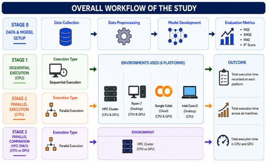
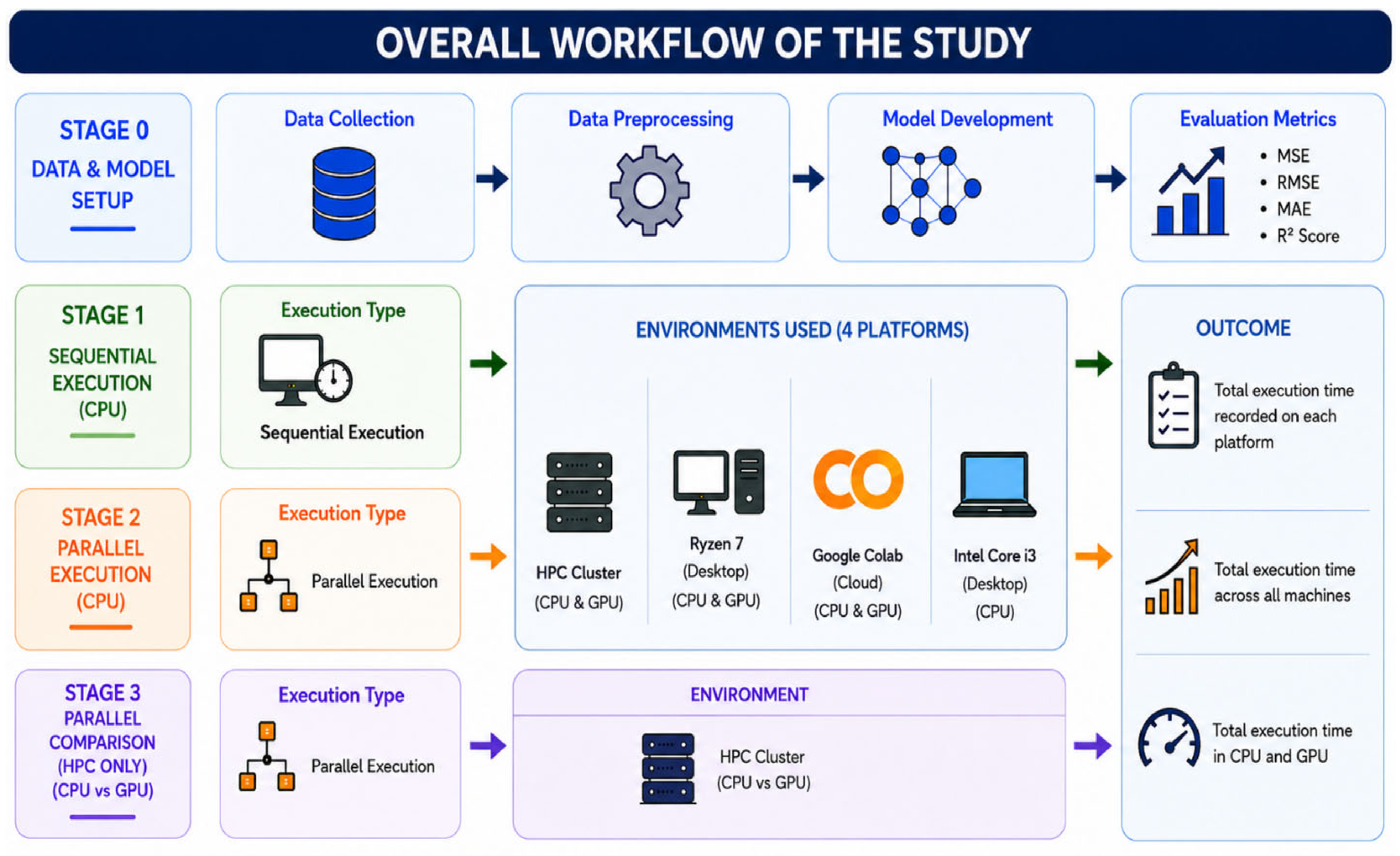
The overall contribution and related work cycle is provided in Figure 1. It provides knowledge and understanding related to the work done, machines and methodologies used and overall results obtained.
Figure 1.
Overall contribution of this study.
Additionally, it demonstrates the overall workflow of the study conducted to evaluate the performance of LSTM models under different computational environments and execution strategies for the largest workloads climatic time-series data. The study was conducted in several phases.
In Stage 0, 4758 observations to 47,480 observation climatic dataset containing the variables T_MED, FF_MED, and RG_TOT were collected and prepared for modeling. Data preprocessing included date parsing, variable selection, Min–Max normalization, and reshaping of the dataset into the three-dimensional structure required for LSTM input. A sequential LSTM architecture consisting of an LSTM layer with 50 units, a dropout layer (0.2), and a dense output layer was developed to predict individual climatic variables. Model performance was evaluated using Mean Squared Error (MSE), Root Mean Squared Error (RMSE), Mean Absolute Error (MAE), and the coefficient of determination (R2).
Stage 1 focused on baseline sequential CPU execution, where variables were trained one after another, which is called sequential execution. Experiments were conducted across four platforms: AMD Ryzen 7 desktop, Intel Core i3 desktop, HPC cluster using SLURM, and Google Colab cloud environment.
In Stage 2, multiprocessing-based parallel CPU execution was implemented, enabling simultaneous training of the three climatic variables. The same four computational environments were used to ensure accurate comparison. Parallel execution significantly reduced training time and improved resource utilization compared to the sequential approach.
Stage 3 investigated CPU versus GPU parallel execution on two platforms: the HPC cluster. Multiple dataset sizes ranging from small to extra-large were evaluated to analyze scalability. Results indicated that GPU acceleration consistently outperformed CPU execution, particularly for larger datasets, where the speedup increased substantially with dataset size.
Finally, Stage 4 involved comprehensive result collection and comparative analysis. Execution times, resource utilization, and model performance metrics were analyzed across all environments and dataset scales. The study further evaluated scalability, computational efficiency, and cost-effectiveness of CPU and GPU implementations for deep-learning-based climatic data.
3. Methodology
3.1. Dataset Description
The real-world dataset was obtained from a weather station in Pinhao, in northern Portugal, covering the period from 1 January 2010 to 31 December 2022. The original dataset contains 4748 observations over 13 years. For controlled computational workload scaling, the dataset was replicated to generate larger synthetic workloads. Table 1 reports the corresponding number of observations and workload sizes used in the experiments.
Table 1.
Characteristics of the dataset.
The larger dataset sizes represent synthetic workload expansions generated by repeatedly replicating the original 13-year dataset. Therefore, the reported durations from 9497 to 47,480 years indicate equivalent workload sizes rather than additional real-world observations.
This dataset contains various meteorological variables relevant to long-term environmental time-series data, which are presented in Table 2. The data have a daily frequency and, in their current form, have no known gaps or flaws.
Table 2.
Variables used from the dataset.
The dataset consists of daily aggregated measurements of mean air temperature (T_MED), mean wind speed (FF_MED), and total global radiation (RG_TOT). These variables were selected because of their different temporal behaviors; wind speed and global radiation present greater intermittency and uncertainty while temperature presents considerable seasonal regularity. This diversity provides a robust testbed for evaluating LSTM models across multiple levels of temporal complexity.
3.2. Data Preprocessing
The original climatic dataset, consisting of 4748 observations spanning 13 years, was synthetically expanded by replicating the original time-series to generate datasets containing up to 47,480 observations. The same preprocessing procedure, LSTM architecture, and training hyperparameters were maintained across all dataset sizes and computational environments. The selected climatic variables were processed independently, and the date column was converted into datetime format. Min–Max normalization was applied separately to each variable using the complete dataset before model training; no explicit chronological training–testing split was performed. The normalized data were reshaped into the three-dimensional input structure required by the LSTM network (samples, time-steps, and features). A single timestep and a single feature were used without a sliding window to maintain a simple and consistent computational workload across the sequential and parallel execution modes. Each model was trained for 40 epochs with a batch size of 32 and a validation split of 10%. This configuration limits the temporal dependencies learned by the LSTM and is acknowledged as a methodological limitation. Since the expanded datasets contain replicated observations rather than new independent climatic measurements, the experiments primarily evaluate computational execution time rather than independent forecasting performance. The same model architecture, training hyperparameters, and preprocessing procedure were used in both execution modes to support a consistent comparison of their execution times.
3.3. Experimental Environments
The experiment was conducted in heterogeneous hardware environments to address the differences between conventional machines and high-performance computing. These included a local PC (Ryzen 7, 16 GB RAM) reference local machine, an older lower-end system Intel Core i3 processor, Google Colab included as a cloud-based environment, and, for HPC system, Deucalion. Another experiment has been executed as HPC jobs via SLURM scripts, with specified computational resources (CPUs, GPU memory, and execution time). Complete details regarding hardware description are provided in Table 3.
Table 3.
Hardware description.
The experiments were implemented in Python using NumPy, Pandas, TensorFlow, parallel techniques. The same version of model architecture and training were maintained across all environments to confirm fair comparison. This methodology evaluates the advantages of HPC setup for large-data performance of LSTM model during data-intensive situations.
3.4. LSTM Model
The implemented model was based on a Long Short-Term Memory (LSTM) neural network architecture designed for time-series prediction tasks which used CPU and GPU processors. The architecture consisted of a single LSTM layer containing 50 hidden units, followed by a dropout layer with a dropout rate of 0.2 to reduce overfitting, and a fully connected dense output layer with one neuron for continuous value prediction.
The CPU-based LSTM implementation used the ReLU activation function in the original experiments, while the GPU-based implementation used the hyperbolic tangent (tanh) activation function. Therefore, the CPU–GPU comparison should be interpreted as an end-to-end comparison of the tested computational implementations rather than as a strictly controlled hardware-only comparison. The CPU-based model accepted input data reshaped into a three-dimensional format corresponding to (samples, timesteps, and features). The model was trained using the Adam optimization algorithm with a learning rate of 0.001 and the Mean Squared Error (MSE) loss function. Training was performed for 40 epochs with a batch size of 32, while 10% of the training data was reserved for validation during the learning process. For the GPU experiments, the tanh activation function was used to enable the optimized GPU implementation. Because the CPU and GPU experiments used different activation functions, implementation-level factors may contribute to the observed performance differences in addition to hardware characteristics.
Prior to training, all input variables were normalized using the Min–Max normalization technique to improve training stability and convergence efficiency. Model performance was evaluated using Mean Squared Error, Root Mean Squared Error, Mean Absolute Error, and the coefficient of determination (R2 score). The same LSTM architecture, hyperparameters, preprocessing strategy, and evaluation procedure were consistently maintained across all computational platforms to ensure fairness and reproducibility in the experimental comparison.
3.5. Execution Strategies and Computational Optimization
In this experiment, two execution strategies were considered: non-parallel execution and parallelized execution. In the sequential approach, model training was performed sequentially using a single process, without distributing the workload across multiple computational resources. In parallelized execution, training tasks were distributed independently across available CPU cores and GPU resources, using optimized configurations such as SLURM scheduling in the HPC environment.
Initially, the experiments were conducted using sequential execution to establish a computational recourse and quantify the inherent scalability gaps of LSTM training for large dataset size. In this approach, model training used single process per experiment, without distributing workloads across multiple CPUs. The computational workload was progressively increased from the original 4748 observations to larger synthetic workloads, corresponding to 13–130 workload-equivalent years. It was observed from the obtained result of using sequential execution that total program execution time linearly increased according to the size of the dataset. In this case, the experiment was manageable for small datasets, but the training time became higher for medium datasets and larger datasets. The largest workload time was measured from the start of the computational workload until completion of the defined training task. The reported timing therefore reflects the operations included within the implemented timing boundary. Preprocessing, process creation, model initialization, training, and evaluation were included/excluded according to the placement of the timing function in the experimental implementation. Timing measurements were used consistently across the compared execution strategies.
While this approach was manageable for smaller datasets, the training time became significantly high for medium and larger datasets. The dataset exceeded approximately 14,244 observations where training time became long even on powerful local systems. Considering those constraints, parallelization was introduced not only as an optimization strategy but also a practical necessity for conducting larger-scale experiments within the available execution-time limits. Scaling the dataset to larger sizes was not suitable within execution time limits without parallelization.
In this work, a task-level parallelization approach was adopted. Instead of modifying the internal structure of the LSTM model, multiple independent training processes were executed simultaneously. Sequential execution used fewer CPU resources and lower utilization of CPU. On the other hand, parallel execution utilized CPU as multiple cores and higher CPU, resulting in shorter training time. Each process handled a separate training task, and no communication or data sharing occurred between them. This ensures that the learning behavior of the model remains unchanged.
The results indicate that parallelization does not affect computational efficiency, particularly execution time, but it remained consistent of predictive performance values, RMSE, MSE, and MAE. In this way, the comparison remains transparent and fair for an ideal experiment.
To better understand the role of parallelization in this study, Table 4 summarizes the key differences between sequential and parallel execution strategies.
Table 4.
Sequential vs. parallel execution strategies.
The results in Table 4 indicate that parallelization improves computational efficiency and scalability, primarily by reducing execution time rather than changing the model’s learning process. Table 5 discusses used configuration and comparison between Sequential LSTM and Parallel LSTM.
Table 5.
Sequential and parallel execution configuration.
The sequential implementation processes the three climatic variables consecutively within a single Python process, whereas the parallel implementation launches three separate worker processes using Python multiprocessing. Threading configurations were explicitly specified in the parallel implementation but not in the sequential implementation. Therefore, the comparison represents the execution performance of the two implemented configurations, rather than a strictly controlled comparison under identical CPU-thread settings. The actual number of active execution threads was not independently measured.
3.6. Parallelization Strategy
HPC systems are designed to execute computationally intensive workloads using multiple processing cores concurrently. To maximize the capability of HPC systems such as Deucalion, it is important to write code that can perform tasks in parallel rather than sequentially. Dividing computational tasks into smaller independent processes that can be executed simultaneously with multiple workers is called parallelization [23]. Parallelization is essential to making optimal use of high-performance computing platforms. Several parallelization strategies are used in HPC, like Message Passing Interface (MPI), data parallelization, task parallelization, etc. Choosing the right strategy is one of the important phases for developers. The structure of the problem and the resources that are available (CPU, GPU, and RAM) are two factors that should be considered when selecting the appropriate strategy, whether it be task-level, data-level, or MPI-based.
In our experiments, parallelization was implemented using a task-level execution approach, in which multiple independent LSTM training tasks were executed concurrently across the available CPU resources. The three climatic variables (T_MED, FF_MED, and RG_TOT) were treated as three independent training tasks, with Python multiprocessing used to launch one separate process for each variable in the CPU-parallel experiments. Task-level parallelism allows independent computational tasks to be assigned to available computing resources and executed concurrently, making it suitable for the largest workload computing environments [22]. This approach follows an embarrassingly parallel strategy because the individual training tasks do not share model parameters, gradients, or intermediate training states. Thus, three worker processes were launched to train the respective LSTM models independently, with process execution managed by the operating system and, in HPC experiments, by SLURM where applicable. This represents task-level parallelism rather than distributed training of a single LSTM model.
Each task was executed as an independent process using Python multiprocessing execution. The internal structure of the LSTM model remained unchanged, and no distributed TensorFlow or MPI-based training was applied. Instead, parallelization was performed at the application level by simultaneously launching multiple independent training jobs.
On the HPC system, Python multiprocessing-based independent training jobs were scheduled across CPU cores and GPU devices through SLURM-managed job submission, which allowed parallel execution. This approach benefits from dedicated computational resources, optimized memory bandwidth, and high-throughput interconnects.
On the Ryzen 7 workstation, parallel execution was implemented using Python’s multiprocessing framework, allowing multiple training processes to utilize available CPU cores within a single node. Explicit thread control was applied to prevent oversubscription and runtime instability, particularly related to OpenMP and LLVM-based threading.
On the Intel Core i3 system, the same parallelization strategy was used, although parallel execution was limited by hardware constraints but followed the same task-level strategy, enabling consistent methodological comparison.
For Google Colab, in this environment parallel execution in Google Colab was implemented using a modified version of the HPC parallelization code without changing LSTM architecture, training process or assessment measures. The performance of the same parallelized AI job under various system-level limitations could be directly evaluated using this architecture. Parallelization methods across different platforms are provided in Table 6.
Table 6.
Parallelization method across different platforms.
It is important to note that this approach does not modify the LSTM learning algorithm or gradient computation. Therefore, accuracy metrics (MSE, RMSE, MAE, and R2) remain unaffected. The parallelization strategy exclusively impacts execution time through improved hardware utilization.
3.7. Evaluation Metrics
The predictive performance of the LSTM model was evaluated using standard regression error metrics. In particular, the difference between predicted and actual values or target variables was assessed using RMSE, MAE, and MSE. As a result, these measures are widely used in time-series forecasting studies due to their ability to capture different aspects of prediction error.
Let denote the actual observed value and represent the corresponding predicted value for the -th observation, with being the total number of samples. The evaluation metrics are defined as follows:
Mean Squared Error (MSE)
Here, MSE is the value of average of the squared differences between predicted and actual values. The squaring process penalizes larger error effectively and makes outliers sensitive. RMSE is calculated as:
RMSE is defined as the square root of MSE. It represents errors in original data units, which makes it easier to understand and interpret prediction errors because larger RMSE values indicate the prediction error for a model and poorer model [6]. MAE is calculated as:
MAE calculates the average of the mean absolute difference between actual and predicted values. Unlike MSE, it is less sensitive to outliers compared to MSE.
For every target variable (T_MED, FF_MED, and RG_TOT), these evaluation metrics were calculated separately for every experimental setup, including varying dataset sizes, hardware platforms, and execution modes (parallel and sequential). A thorough evaluation of the model’s performance is guaranteed by using a variety of complementing measures that capture the size and distribution of prediction errors.
Additionally, a fair and trustworthy comparison of predicted performance is made possible by the uniform use of these measures throughout all tests, guaranteeing that any observed variations in outcomes may be ascribed to computational factors rather than inconsistent evaluation technique.
4. Results and Discussion
4.1. Sequential Execution Analysis
The study systematically evaluates the execution time of LSTM-based time-series models over the heterogeneous computing setup. Sequential execution performs tasks one after another in a single-process manner. The particular focus of this experiment was to benchmark the total execution time to complete the task under increasing workload of LSTM model. Three climatic variables are trained individually in a consecutive manner, where the training of one variable starts only after the previous variable has completed a task. This approach utilizes only limited computational resources at a time, resulting in longer execution times as no simultaneous computation occurs. Sequential execution conducted a primary experiment for evaluating computational performance, which can lead to comparing parallel execution approaches.
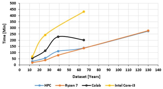
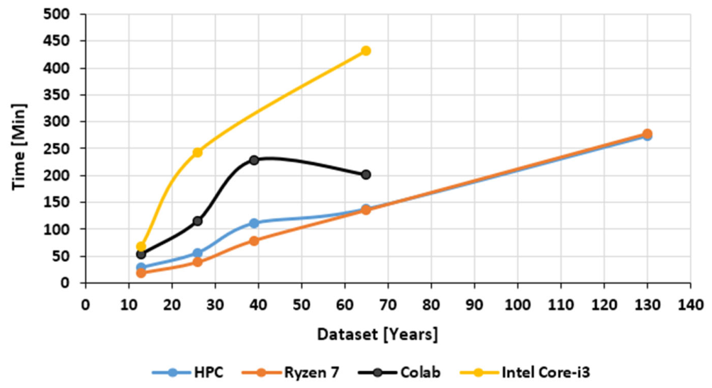
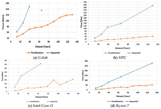
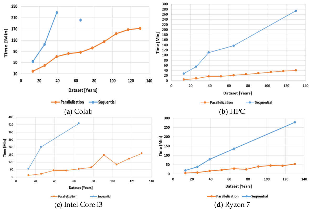
Figure 2 represents the result of sequential execution over different machines. The experiments were conducted using the same LSTM-based time-series prediction script across four computational environments to ensure a fair and consistent comparison of computational performance. The implemented neural network architecture remained identical in every environment, including the number of layers, neuron configuration, dropout rate, activation function, optimizer settings, batch size, and training epochs. The model consisted of an LSTM layer with 50 units using the ReLU activation function, followed by a dropout layer of 0.2 and a dense output layer.
Figure 2.
Sequential execution comparison in different machines.
The Adam optimizer with a learning rate of 0.001 was applied, while training was performed using a batch size of 32 for 40 epochs. The same dataset, preprocessing procedure, normalization method, and evaluation metrics (MSE, RMSE, MAE, and R2 score) were maintained throughout all experiments. All experiments were conducted using LSTM model and training procedure with sequential execution applied at task level to confirm methodological consistency across the different hardware environments. This section presents the results of CPU-based sequential execution and examines the influence of hardware limitations on execution time. Figure 3 illustrates that sequential execution highlights the significant impact of computational limitations across different hardware environments on CPU processors.
Figure 3.
Parallel vs. sequential execution across all environments.
Execution time varied substantially across dataset sizes and computing platforms. Although, the performance differences are clearly observable in the graph. Ryzen 7 processor was demonstrated as faster for small to moderate data size during sequential execution compared to HPC because it has higher turbo clock speed, stronger single core boost, faster local memory access and lower system latency. HPC manages several simultaneous tasks and high-throughput workloads and multi-user resource sharing can be slower than Ryzen 7 for small to medium data size. However, for a larger dataset that contains 47,480 observations, HPC is faster than Ryzen 7. Ryzen 7 is better for single-core performance and lightweight workload performance.
The results are consistent with previous studies indicating that computing architecture influences the feasibility and efficiency of deep learning workloads.
The HPC and Ryzen 7 systems exhibit comparable runtimes, while Google Colab and Intel Core i3 show noticeably higher execution times, indicating limited computational efficiency even at a small scale.
However, total execution time increased proportionally with the growth of data size across the platform; therefore, the experiments were not continued with all available dataset-size scales across Google Colab and Intel Core i3. The experiments were discontinued by Colab and Intel Core i3 in medium to large datasets due to their longer execution running time. Instead, the evaluation conducted sequentially on datasets of increasing size, including a small-scale (14,244 observations), medium-scale (23,740 observations), and the largest workload (47,480 observations) configuration for HPC and Ryzen 7 machines.
When compared to HPC and Ryzen 7, this increase is especially noticeable for lower-performance systems like Intel Core i3 and Google Colab, where runtime increases significantly. Even high-performance systems begin to exhibit scalability constraints, with execution times nearly doubling as the dataset size increases.
Sequential LSTM training did not scale efficiently as dataset size increased. This method is not feasible for medium to the largest workload datasets due to the quick increase in execution time. Consequently, further experiments using sequential were discontinued beyond this point. These observations motivated the transition to parallelization strategies, which aim to improve computational efficiency and enable scalable processing of larger datasets without compromising model performance.
4.2. Parallel Execution Performance
To evaluate computational efficiency, task-level parallelism was implemented using Python multiprocessing, where three independent climatic variables were trained concurrently on different CPU cores. Each process independently trained one LSTM model for one climatic variable, with no parameter or gradient sharing between the models.
In addition, both CPU and GPU nodes were evaluated on the HPC system to examine the impact of hardware acceleration. Parallel computing in HPC is useful to make software run faster and more efficiently [22]. Parallel computing techniques solve big problems very fast on supercomputers by splitting their jobs into small tasks at the same time [25].
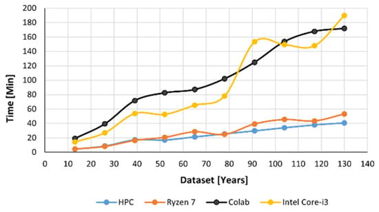
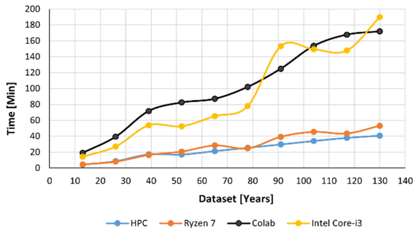
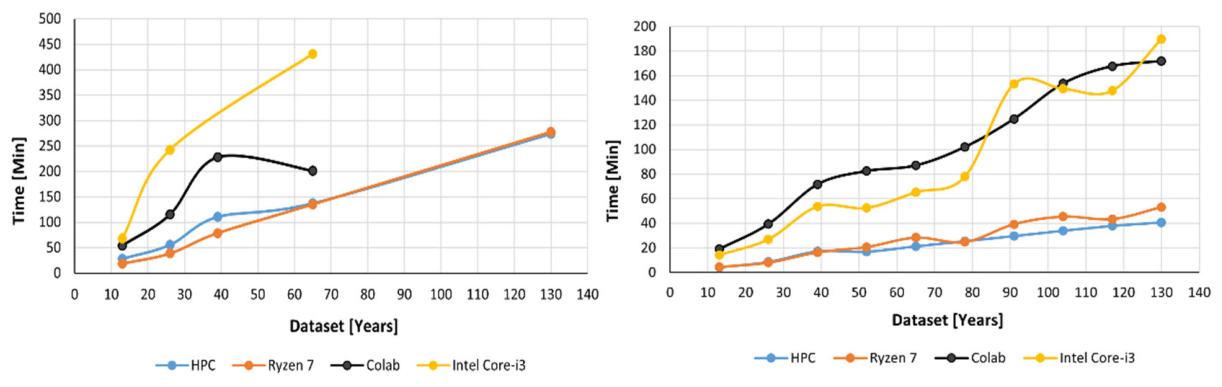
The primary objective of the work was to analyze how total execution time and computational efficiency vary while the growth of the dataset at the same deep learning workload is deployed on heterogeneous hardware platforms. Parallel multiprocessing uses three CPU cores independently of three variables, where each process trained one climate variable concurrently. Figure 4 represents the graph result of using parallelization across all different hardware environments.
Figure 4.
Parallelization across all machines.
Across all tested platforms, parallelization methods significantly reduce the total execution time compared with sequential execution, especially for medium to large datasets. Among the CPU-based systems the HPC consistently demonstrated superior scalability and stability across all over the dataset length. However, under multiprocessing parallel execution, the HPC platform significantly outperformed across all dataset sizes due to its multi-core scalability, memory bandwidth and optimized resource allocation for concurrent workloads. HPC is typically designed with many physical CPU cores, larger shared memory, server-grade CPUs, optimized task scheduling and reduced contention under heavy workloads. Figure 5 represents the comparison between sequential and parallelization.
Figure 5.
Sequential vs. parallelization.
The AMD Ryzen 7 machine also exhibited good performance compared to execution times. This workstation also performed well, supported by its eight-core configuration and 16 GB of RAM. However, as the dataset increased the Ryzen 7 machine required additional system adjustments including virtual memory allocation and thread configuration. This indicates that, although Ryzen 7 has a capable processor, it has some structural limitations.
The Intel Core i3 system required more execution time than the Ryzen 7 and HPC systems in both sequential and parallel experiments. It required longer execution times in both sequential and parallel experiments compared to all three other environments. However, the platform successfully executed the same model architecture, dataset, hyperparameters, and multiprocessing strategy, ensuring fairness in comparative benchmarking for very small datasets.
Google Colab provides shared and virtualized computational resources and the observed execution times reflect the performance characteristics of cloud-based CPU resources under task-level parallel execution. Colab is not fully recommended for TensorFlow-based Python multiprocessing execution because multiprocessing within notebook-based cloud environments can affect process spawning instability, deadlocks, memory contention, and unexpected runtime crashes during LSTM training.
In contrast, Google Colab and the Intel Core i3 system showed limited scalability. Google Colab followed the same parallelization strategy, which was unable to handle larger datasets efficiently due to shared-resource constraints, restricted memory availability, and session-level execution limits. The Intel Core i3 system exhibited the slowest execution times overall and became impractical for the largest workload experiments, while the Ryzen 7 system consistently outperformed the Intel Core i3 and Google Colab.
In the parallelized execution setting, a significant improvement in computational efficiency is observed across all platforms. Notably, both the HPC system and the AMD Ryzen 7 workstation demonstrate comparable performance for larger datasets, with execution times of approximately 40.69 s and 53.07 s, respectively. This close performance indicates that modern multi-core consumer-grade processors can effectively leverage parallelization techniques for moderate-scale workloads.
Nevertheless, HPC system maintained a performance advantage, particularly as dataset size increased. Its improved CPU architecture, more core scalability, and more effective resource management in a high-performance computing environment are the reasons for its supremacy. These findings unequivocally demonstrate the effectiveness of combining HPC equipment with CPU-based parallelization to speed up deep learning workloads.
Considering the obtained results, this study further explored the GPU acceleration on HPC systems following parallelization techniques; however, next experiments towards HPC environments only sing parallelization techniques. This decision has been made to explore the necessity of accessing the advantages of specialized hardware, like GPUs, in handling the largest workloads, LSTM training workloads and to further reduce execution time. Based on this result, next investigations compare the performance of CPUs and GPUs in parallelized settings, with special attention to the scalability benefits provided by HPC systems.
4.3. CPU vs. GPU Performance (HPC Only)
In the final stage of the experiment the analysis focuses on the comparison of CPU and GPU execution time within HPC platform under parallelization conditions. Since Ryzen 7 has good processor NVIDIA GeForce RTX 4050, however, it was not sufficient for efficient parallel execution of multiple LSTM training tasks simultaneously on a single processor. Since all variables would compete for the same GPU resources, this could introduce GPU contention, memory-sharing overhead, and inconsistent execution behavior. Therefore, GPU-based experiments were conducted on the HPC platform, where multiple GPU resources enabled distributed array-based execution and more suitable parallel workload allocation for fair performance evaluation.
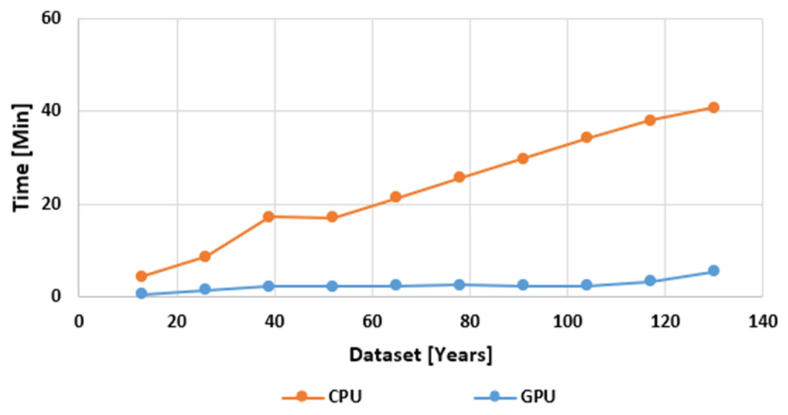
As demonstrated in Figure 6, the experiment was conducted on 4748 to 47,480 observation datasets using parallel computing and CUDA [31]. Although both CPU- and GPU-based implementation are used in LSTM architecture and preprocessing methodology, several differences existed between the scripts due to hardware requirements. The GPU-based model employed the tanh activation function to accelerate cuDNN operations on NVIDIA GPUs. The GPU version relied on TensorFlow’s internal GPU acceleration for parallel tensor computations. On the other hand, the CPU-based implementation parallelism used multiprocessing techniques across variables. Note that the primary objective of this experiment is to analyze the computational performance (total execution time) of AI workloads across heterogeneous hardware platforms, rather than to optimize predictive accuracy or neural network architecture design. With the increasing number of dataset sizes, the execution time increases relatively while using parallelism on a CPU-based node. CPU execution runtimes for the largest workload datasets are higher compared to GPU nodes. GPU demonstrates remarkably low and stable execution times even for the largest workload datasets. This result addresses the effectiveness of GPU acceleration for deep learning workloads, especially for models with high computational demands like LSTM. GPU libraries CUDA and cuDNN accelerate training and model inference based on GPU architecture in the frameworks like TensorFlow 2.13.1 and PyTorch.
Figure 6.
Execution time of CPU- and GPU-based across different workload sizes.
This behavior aligns with existing studies explaining that GPU architecture consisted of highly optimized libraries such as cuDNN, significantly accelerating LSTM training and inference. Previous research has shown that cuDNN-optimized LSTM implementations outperform traditional CPU-based approaches across multiple deep learning frameworks [17,20,33]. Figure 6 shows lower execution times for the GPU-based implementation; however, this is not a fully controlled CPU–GPU comparison because the implementations differ in hardware, software, and activation function.
Overall, the results show that the GPU-based implementation achieved lower execution times for the tested largest LSTM workloads.
The observed performance improvement is largely attributed to the use of NVIDIA’s Compute Unified Device Architecture (CUDA) and the CUDA Deep Neural Network (cuDNN) library. CUDA enables massive parallelism by allowing thousands of lightweight threads to execute simultaneously on the GPU [20], making it highly suitable for matrix operations and sequence-based computations inherent in LSTM models. NVIDIA’s CUDA architecture is the stronger processors enable of HPC applications [19]. Furthermore, cuDNN provides highly optimized implementations of recurrent neural network operations [24], significantly accelerating both forward and backward propagation during training [24]. These optimizations reduce computational overhead and ensure efficient utilization of GPU resources.
In contrast, CPU-based execution, even with parallelization, remains limited by the number of available cores and the sequential nature of certain operations. Although HPC CPUs offer high performance and scalability, they cannot match the level of fine-grained parallelism provided by GPUs. Consequently, the gap in execution time between CPU and GPU widens as the dataset size increases. GPU basically outperformed CPU in deep learning workflow while handling threads simultaneously and best performing them 10× to 100× in data processing [31]. The GPU implementation achieved lower execution time than the CPU implementation under the tested configurations. However, this comparison reflects the combined effect of hardware, software backend, and activation-function differences. Therefore, the observed performance improvement should not be attributed exclusively to the hardware. CPUs are ideal for sequential processing due to their single-threaded performance [26]. Modern GPUs provide massive parallelism through hundreds of cores and thousands of concurrent threads [34].
Overall, these results clearly demonstrate that GPU-accelerated computing within an HPC environment is the most effective approach for the largest workload LSTM training. The combination of parallelization, CUDA-enabled processing, and cuDNN optimizations enables substantial reductions in execution time without compromising predictive accuracy [32], thereby reinforcing the critical role of HPC infrastructure in advancing efficient AI model deployment.
4.4. Repeated Timing Experiments and Statistical Analysis
The original performance evaluation was conducted on 10 datasets of different sizes, and the corresponding results are presented in the existing figures. To further investigate the variability of execution time, additional timing experiments were performed on three representative dataset sizes, small (4748), medium (28,488), and large (47,480), on HPC and Ryzen 7 for parallel execution. Since sequential execution was not conducted for medium and large datasets, therefore, repeated measurements were not performed. Each selected configuration (Parallel execution on HPC and Ryzen 7) was executed three times under the available experimental environment.
For each of these configurations, the mean execution time and sample standard deviation (SD) were calculated, and the 95% confidence interval (CI) was estimated. The resulting statistics are reported in Table 7 and Table 8 of parallel execution on two platform (HPC and Ryzen 7).
Table 7.
Parallel execution on HPC.
Table 8.
Representation of Ryzen 7 parallel execution result.
Each configuration was evaluated in three independent runs. The mean execution time and sample standard deviation (SD) were calculated from the repeated measurements. The 95% confidence intervals (CIs) were calculated using the sample standard deviation and the t-critical value with two degrees of freedom. These statistical results apply only to the CPU-based parallel implementations on the HPC and Ryzen 7 platforms for the three selected dataset sizes.
4.5. Predictive Accuracy Analysis
This section describes the predictive performance impact of LSTM model across the different data sizes or execution platforms. As mentioned earlier, three metric values were performed using RMSE, MSE, and MAE for three target variables: average temperature (T_MED), wind speed (FF_MED), and global radiation (RG_TOT). This stage is significant to verify whether variations in data size or hardware platform impact on the LSTM model.
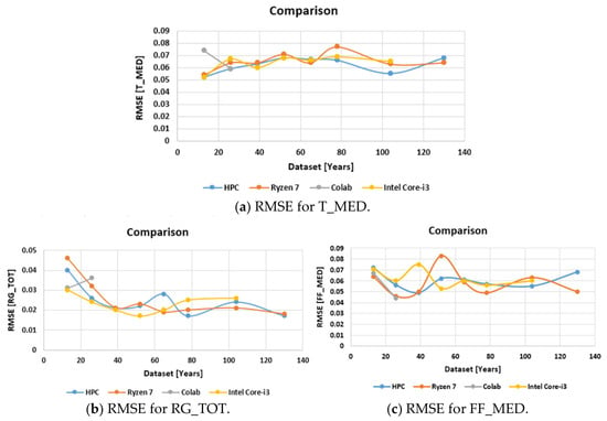
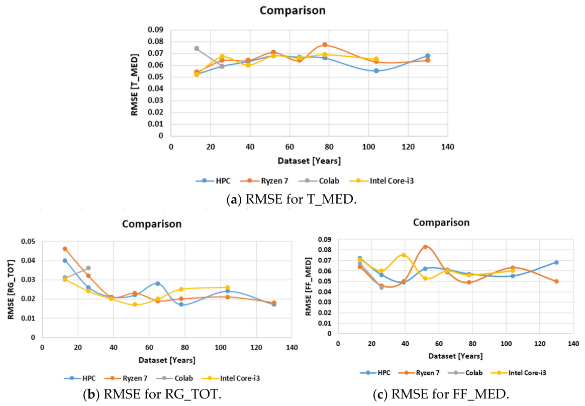
Three target variables were evaluated namely by average temperature (T_MED), wind speed (FF_MED), and global radiation (RG_TOT). The results from Figure 7 is showing that predictive performance remains highly stable across all tested hardware platforms, including the HPC system, AMD Ryzen 7 workstation, Intel Core i3 processor, and Google Colab environment.
Figure 7.
RMSE performance with parallelization across all machines (CPU).
The results show that predictive performance remains highly stable across all tested hardware platforms, including the HPC system, AMD Ryzen 7 workstation, Intel Core i3 processor, and Google Colab environment. As the size of the dataset increased from 13 to 130 years, RMSE values for each variable fluctuate only within a small range with no systematic degradation observed. This consistency indicates that changes in hardware or application of parallelization do not harm the underlying behavior of the model as identical architectures, hyperparameters, preprocessing steps and training models remained same across all experiments. RMSE values show minor variations across different dataset sizes; however, repeated runs and statistical analysis were not performed to quantify the variability of these results.
In some cases, the original dataset, which is the smallest dataset, achieves the lowest RMSE values. HPC and parallelization strategies dramatically reduced training times and execution times while producing the RMSE values that were almost comparable. The results indicate that the tested parallelization strategies primarily affected computational efficiency, while predictive accuracy remained comparable across the tested configurations. Furthermore, the comparable RMSE values across the three meteorological variables indicate consistent predictive performance across the tested configurations.
4.6. Discussion
This study provides clear insights into how the performance of LSTM models impacts different computational environments. The initial observations are that execution time increases fast with dataset size when parallelization is not used. As LSTM model training involves sequential operations and repeated computation, therefore, this behavior is expected. After utilizing parallelization, the overall performance improved drastically across all platforms. This indicates that the model architecture itself is not the primary limitation but in the way the computations are executed. The training process became more efficient by distributing workload across multiple cores. At the same time the prediction accuracy remained almost constant, which demonstrates that parallelization does not affect the learning process. Another observation is the difference between hardware environments. The AMD Ryzen 7 and HPC performance was relatively close and Intel Core i3 and Google Colab are less suitable for handling medium to large-scale datasets. In contrast, the HPC environment remained stable and efficient performance across all the dataset sizes and maintained the scalability. The larger workload sizes used in this study were generated by replicating the original 13-year dataset. Therefore, these expanded datasets represent controlled computational workload scaling rather than genuinely longer historical observations. Repeated temporal patterns and the absence of new observational variability may affect LSTM memory behavior, convergence characteristics, and measured scalability. Consequently, the scalability results should be interpreted primarily as a computational workload assessment, and their generalizability to larger and more diverse real-world datasets remains limited.
Due to experimental time and resource constraints, repeated timing experiments were conducted for only three representative climate dataset sizes (small, medium, and large) on HPC and Ryzen 7 platform as a parallel execution. Consequently, the original execution-time results for the remaining datasets are retained as single-run measurements. Although the repeated experiments provide an estimate of execution-time variability for the selected dataset sizes across the tested configurations, the findings may not fully characterize timing variability across all ten datasets. Repeated measurements across all dataset sizes would be required to provide a more comprehensive assessment of execution-time variability.
Another experiment was conducted between CPU and GPU execution in the HPC environment. The primary objective was to measure training and total task completion time across different hardware configurations under increasing workloads. The GPU-based implementation achieved lower execution times than the CPU-based implementation, particularly for larger dataset sizes. This improvement reflects the combined effects of hardware, software implementation, and optimized libraries such as CUDA and cuDNN. Since the CPU and GPU implementations used different activation functions, this comparison does not fully isolate hardware effects. The results highlight the importance of selecting appropriate hardware and execution strategies for scaling deep learning workflows. Detailed CPU/GPU utilization, memory consumption, GPU memory usage, speedup, parallel efficiency, and epoch-level timing were not systematically recorded. These measurements would provide a more detailed assessment of resource utilization and computational efficiency.
A limitation of the CPU–GPU comparison is that the implementations used different activation functions (ReLU for CPU and tanh for GPU). The current evaluation primarily considers total execution time and predictive metrics. CPU and GPU utilization, memory usage, GPU memory usage, quantitative speedup, parallel efficiency, throughput, and epoch-level timing were not systematically recorded. This can be considered as a limitation.
5. Conclusions
A comprehensive analysis was presented in this study focusing on LSTM model performance across heterogeneous computing environments. It considered the execution time, scalability and predictive performance across different hardware setups. The experiments were conducted using datasets gradually expanded from 4748 to 47,480 observations, to evaluate how data increasing volume affects computational efficiency.
The experiments started using LSTM sequential models’ execution, which revealed significant limitations in total execution time and scalability. As the growth of the dataset, execution time rapidly grew across all platforms. For the workloads evaluated in this study, sequential execution became increasingly time-consuming as the number of observations increased. Parallel execution reduced the execution time and enabled the completion of the larger experimental workloads within the available computational resources. These findings demonstrate the benefit of task-level parallelization for the tested workload range; however, they should not be interpreted as evidence of scalability to substantially larger real-world datasets or general HPC workloads. Considering this limitation, the motivation raised to adopt parallelization techniques, resulting in a considerable reduction in execution time without compromising model performance. Comparative analysis showed that AMD Ryzen 7 and HPC provided better execution performance for the larger tested workloads than the other evaluated platforms. Repeated experiments for every single dataset with different hardware with multiple independent runs and statistical analysis would provide a more robust assessment of performance variability and are considered an important direction for future work. The GPU-based implementation also achieved lower execution times than the CPU-based implementation on the HPC platform. However, the CPU–GPU comparison was affected by differences in hardware, software backend, activation function, and parallel execution strategy. These measurements would provide a more comprehensive characterization of computational performance and should be included in future evaluations. Future work will extend the evaluation using independently collected larger datasets, controlled CPU–GPU experiments with identical model configurations, repeated runs, detailed resource-utilization measurements, and epoch-level timing. Sliding-window temporal modeling will also be investigated in future work to evaluate richer temporal dependencies and computational scalability. Future work will include evaluating larger and more diverse real-world datasets, exploring advanced LSTM and hybrid models, investigating distributed and multi-GPU parallelization, and assessing energy efficiency and resource utilization. Other architectures, such as GRU and Transformers, will also be considered for broader evaluation across heterogeneous computing environments.
Author Contributions
Conceptualization, T.T.H. and T.P.; methodology, T.T.H. and T.P.; software, T.T.H. and T.P.; validation, T.T.H., C.S. and T.P.; formal analysis, T.T.H., C.S., M.T.A. and T.P.; investigation, T.T.H., C.S., M.T.A. and T.P.; resources, T.T.H., C.S. and T.P.; data curation, T.T.H. and T.P.; writing—original draft preparation, T.T.H. and T.P.; writing—review and editing, T.T.H. and T.P.; visualization, T.T.H. and M.T.A.; supervision, C.S. and T.P.; project administration, T.P.; funding acquisition, T.P. All authors have read and agreed to the published version of the manuscript.
Funding
This research was funded by EUROCC2-NATIONAL COMPETENCE CENTRES IN THE FRAMEWORK OF EUROHPC PHASE 2.
Data Availability Statement
The data presented in this study are available in the article.
Acknowledgments
The authors would like to acknowledge the University of Trás-os-Montes and Alto Douro (UTAD) for providing the opportunity and institutional support to carry out this research project.
Conflicts of Interest
The authors declare no conflicts of interest.
Abbreviations
The following abbreviations are used in this manuscript:
| LSTM | Long Short-Term Memory |
| HPC | High-Performance Computing |
| CUDA | Compute Unified Device Architecture |
| cuDNN | CUDA Deep Neural Network |
| DL | Deep Learning |
| MSE | Mean Square Error |
| RMSE | Root Mean Square Error |
| MAE | Mean Absolute Error |
References
- Lim, B.; Zohren, S. Time-series forecasting with deep learning: A survey. Philos. Trans. R. Soc. A 2021, 379, 20200209. [Google Scholar] [CrossRef] [Scilit]
- Kong, X.; Chen, Z.; Liu, W.; Ning, K.; Zhang, L.; Marier, S.M.; Liu, Y.; Chen, Y.; Xia, F. Deep learning for time series forecasting: A survey. Int. J. Mach. Learn. Cybern. 2025, 16, 5079–5112. [Google Scholar] [CrossRef] [Scilit]
- Li, X.-R.; Ban, X.-J.; Yuan, Z.-L.; Qiao, H.-R. Review on deep learning models for time series forecasting in industry. J. Univ. Sci. Technol. 2022, 44, 757–766. [Google Scholar]
- Hochreiter, S.; Schmidhuber, J. Long short-term memory. Neural Comput. 1997, 9, 1735–1780. [Google Scholar] [CrossRef] [Scilit]
- Graves, A. Supervised sequence labelling. In Supervised Sequence Labelling with Recurrent Neural Networks; Springer: Berlin/Heidelberg, Germany, 2012; pp. 5–13. [Google Scholar]
- Goodfellow, I.; Bengio, Y.; Courville, A.; Bengio, Y. Deep Learning; MIT Press: Cambridge, MA, USA, 2016; pp. 1–800. [Google Scholar]
- Brownlee, J. Deep Learning for Time Series Forecasting; Machine Learning Mastery: Vermont South, Australia, 2018. [Google Scholar]
- Dongarra, J.; Beckman, P.; Moore, T.; Aerts, P.; Aloisio, G.; Andre, J.C.; Barkai, D.; Berthou, J.Y.; Boku, T.; Braunschweig, B.; et al. The international exascale software project roadmap. Int. J. High Perform. Comput. Appl. 2011, 25, 3–60. [Google Scholar] [CrossRef] [Scilit]
- Chapman, B.; Jost, G.; van der Pas, R. Using OpenMP: Portable Shared Memory Parallel Programming; MIT Press: Cambridge, MA, USA, 2007. [Google Scholar]
- Chetlur, S.; Woolley, C.; Vandermersch, P.; Cohen, J.; Tran, J.; Catanzaro, B.; Shelhamer, E. cuDNN: Efficient primitives for deep learning. arXiv 2014, arXiv:1410.0759. [Google Scholar]
- Shi, X.; Gao, Z.; Lausen, L.; Wang, H.; Yeung, D.Y.; Wong, W.K.; Woo, W.C. Deep learning for precipitation nowcasting: A benchmark and a new model. Adv. Neural Inf. Process. Syst. 2017, 30. [Google Scholar] [CrossRef] [Scilit]
- Siami-Namini, S.; Siami Namin, A. Forecasting economics and financial time series: ARIMA vs. LSTM. arXiv 2018, arXiv:1803.06386. [Google Scholar]
- Appleyard, J. Optimizing Recurrent Neural Networks in cuDNN 5. NVIDIA Technical Blog, 6 April 2016. Available online: https://developer.nvidia.com/blog/optimizing-recurrent-neural-networks-cudnn-5/ (accessed on 26 April 2026).
- Saha, A.; Rahman, M.; Wu, F. Benchmarking CPU vs. GPU on LSTM Model Using Groundwater Dataset. In Proceedings of the SoutheastCon 2025, Fort Lauderdale, FL, USA, 20–23 March 2025. [Google Scholar]
- Tasnim, T.; Rahman, M.; Wu, F. A comparative analysis of CPU and GPU-based cloud platforms for CNN binary classification. In Proceedings of the 2024 IARIA Annual Congress on Frontiers in Science, Technology, Services, and Applications, Nice, France, 9–13 June 2024. [Google Scholar]
- Assali, T.; Ayoub, Z.T.; Ouni, S. Multivariate LSTM for execution time prediction in HPC for distributed deep learning training. In Proceedings of the 2024 IEEE 27th International Symposium on Real-Time Distributed Computing (ISORC), Tunis, Tunisia, 22–25 May 2024. [Google Scholar]
- Alaei, M.; Yazdanpanah, F. A survey on heterogeneous CPU–GPU architectures and simulators. Concurr. Comput. Pract. Exp. 2025, 37, e8318. [Google Scholar] [CrossRef] [Scilit]
- Buber, E.; Diri, B. Performance analysis and CPU vs GPU comparison for deep learning. In Proceedings of the 2018 6th International Conference on Control Engineering & Information Technology (CEIT); IEEE: New York, NY, USA, 2018; pp. 1–6. [Google Scholar]
- Hasnaine, Q.R.; Fouda, M.M.; Chiu, S.C. GPU vs. CPU: A comparative study of performance, architecture, and NVIDIA’s innovations in modern computing. In Proceedings of the 2025 IEEE 4th International Conference on Computing and Machine Intelligence (ICMI); IEEE: New York, NY, USA, 2025; pp. 1–6. [Google Scholar]
- Choquette, J.; Gandhi, W. NVIDIA A100 GPU: Performance & innovation for GPU computing. In Proceedings of the 2020 IEEE Hot Chips 32 Symposium (HCS); IEEE: New York, NY, USA, 2020; pp. 1–43. [Google Scholar]
- Curzel, S.; Ferrandi, F.; Fiorin, L.; Ielmini, D.; Silvano, C.; Conti, F.; Bompani, L.; Benini, L.; Calore, E.; Schifano, S.F.; et al. A survey on design methodologies for accelerating deep learning on heterogeneous architectures. arXiv 2023, arXiv:2311.17815. [Google Scholar]
- Nguyen, T.D.; Park, J.H.; Hossain, M.I.; Hossain, M.D.; Lee, S.-J.; Jang, J.W.; Jo, S.H.; Huynh, L.N.T.; Tran, T.K.; Huh, E.-N. Performance analysis of data parallelism technique in machine learning for human activity recognition using LSTM. In Proceedings of the 2019 IEEE International Conference on Cloud Computing Technology and Science (CloudCom), Sydney, Australia, 2–4 December 2019. [Google Scholar]
- Helstab, P. A Systematic Review on Integrating Parallel Computing Techniques for High-Performance Computing: Challenges and Best Practices. Aktuelle Themen der Softwaretechnik aus Forschung und Praxis. 2023. Available online: https://helstab.cc/static/A_Systematic_Review_on_Integrating_Parallel_Computing_Techniques_for_High-Performance_Computing_Challenges_and_Best_Practices.pdf (accessed on 19 October 2026).
- Yi, X. A study of performance programming of CPU, GPU accelerated computers and SIMD architecture. arXiv 2024, arXiv:2409.10661. [Google Scholar]
- Bai, X.; Zhou, J.; Wang, Z. HPC cluster task prediction based on multimodal temporal networks with hierarchical attention mechanism. Computers 2025, 14, 335. [Google Scholar] [CrossRef] [Scilit]
- Mittal, S.; Vetter, J.S. A survey of CPU-GPU heterogeneous computing techniques. ACM Comput. Surv. 2015, 47, 1–35. [Google Scholar] [CrossRef] [Scilit]
- Dan, A.; Patil, U.; De, A.; Manuraj, B.N.M.; Ramachandran, R. CPU and GPU based acceleration of high-dimensional population balance models via the vectorization and parallelization of multivariate aggregation and breakage integral terms. Comput. Chem. Eng. 2025, 196, 109037. [Google Scholar] [CrossRef] [Scilit]
- Karyakarte, M.; Kundnani, H. Performance optimization of highly computational tasks using CUDA. Int. J. Eng. Res. Technol. 2013, 2, 1–5. [Google Scholar]
- Grahn, H.; Lavesson, N.; Lapajne, M.H.; Slat, D. CudaRF: A CUDA-based implementation of Random Forests. In Proceedings of the 2011 9th IEEE/ACS International Conference on Computer Systems and Applications (AICCSA); IEEE: New York, NY, USA, 2011; pp. 95–101. [Google Scholar]
- Krizhevsky, A.; Sutskever, I.; Hinton, G.E. ImageNet classification with deep convolutional neural networks. In Proceedings of the 25th International Conference on Neural Information Processing Systems (NeurIPS 2012), Lake Tahoe, NV, USA, 3–6 December 2012. [Google Scholar]
- Moustafa, N. A new distributed architecture for evaluating AI-based security systems at the edge: Network TON_IoT datasets. Sustain. Cities Soc. 2021, 72, 102994. [Google Scholar] [CrossRef] [Scilit]
- Boukili, M.; Jebbor, N.; Errajraji, K.; Elbathaoui, M. CNN model acceleration and optimization: CPU and GPU performance analysis and evaluation for multiclass classification. Array 2026, 30, 100746. [Google Scholar] [CrossRef] [Scilit]
- Niteesh, L.; Ampareeshan, M.B.; Murugan, S. Optimizing machine learning models with CUDA: A comprehensive performance analysis. In Proceedings of the 2025 3rd International Conference on Communication, Security, and Artificial Intelligence (ICCSAI); IEEE: New York, NY, USA, 2025; pp. 831–836. [Google Scholar]
- Kirimtat, A.; Krejcar, O. GPU-Based Parallel Processing Techniques for Enhanced Brain Magnetic Resonance Imaging Analysis: A Review of Recent Advances. Sensors 2024, 24, 1591. [Google Scholar] [CrossRef] [Scilit]

Disclaimer/Publisher’s Note: The statements, opinions and data contained in all publications are solely those of the individual author(s) and contributor(s) and not of MDPI and/or the editor(s). MDPI and/or the editor(s) disclaim responsibility for any injury to people or property resulting from any ideas, methods, instructions or products referred to in the content. |
© 2026 by the authors. Licensee MDPI, Basel, Switzerland. This article is an open access article distributed under the terms and conditions of the Creative Commons Attribution (CC BY) license.