


Abstract
The traditional dynamic window approach (DWA) cannot perceive semantic risk levels in substation environments. We propose a lightweight semantic navigation scheme that takes a prior semantic map as input, applies differentiated safety inflation to semantic regions according to category (danger zones dsafety × 1.5, secondary forbidden zones dsafety × 0.5), and fuses them into the Nav2 costmap via per-cell maximum fusion. The standard DWA thereby gains hierarchical avoidance capability at the costmap representation level, without modifying the DWA planner core. Gazebo simulations were performed with 80 runs per group, each collected under an independent simulation restart. Compared with the conventional baseline, the proposed scheme increases the minimum clearance from the robot silhouette to the physical equipment boundaries from 0.42 m to 0.66 m and the minimum signed clearance to the boundary of the pure semantic forbidden zone—a physically empty region marked only in the semantic layer—from −0.36 m (penetration in every run) to +0.46 m. Center-point entries into semantic forbidden zones are reduced to zero (80/80 → 0/80), at the cost of an 11.8% increase in path length. Statistical significance is confirmed by Welch’s t-tests with Holm–Bonferroni adjustment and by non-parametric Mann–Whitney U tests. Comparison with the Nav2 native KeepoutFilter shows that hard boundaries without soft buffering degrade DWA traversability: the right-angle expanded mask failed in all 50 attempts, and the rounded expanded mask succeeded in only 48% (24/50), whereas the proposed scheme maintained 100% (80/80). Ablation, noise, and offset–delay experiments with 30 runs per condition further validate the robustness of the scheme. In the exploratory new-start-point comparison (n = 10 per group), differentiated inflation matched uniform large inflation at the highest-risk device (0.764 m vs. 0.771 m) while keeping the path 2.6% shorter. The proposed scheme provides a loosely coupled, easily deployable semantic navigation safety enhancement for substation inspection robots.
1. Introduction
Mobile robots are widely used in intelligent warehousing, campus logistics, and substation inspection, where autonomous navigation capability is essential. As the core module of navigation systems, path planning must generate safe and efficient driving paths in complex environments [1]. Traditional frameworks represent the environment with two-dimensional grid costmaps, whose theoretical foundation can be traced back to the occupancy grid map [2]. The cost values depend only on physical obstacle perception from sensors such as LiDAR, without any understanding of semantic attributes in the environment. The dynamic window approach (DWA) samples in velocity space and scores candidate trajectories using an evaluation function to achieve real-time local dynamic obstacle avoidance [3], but it only reacts to occupied grid cells and cannot distinguish semantic risk levels between different obstacles.
With the development of visual sensing and deep learning, research on mobile robot navigation has incorporated semantic information [4]. Real-time object detection models such as YOLO have been widely applied in robot visual perception [5]. Semantic information can tell the robot “what is ahead” rather than only “how far it is.” Existing studies have verified the feasibility of introducing semantic information into robot navigation systems [6], and research on semantic mapping has become relatively mature [7,8]; some works combine object detection with visual SLAM to construct semantic maps [8]. In substation inspection scenarios, deep learning-based obstacle avoidance methods have demonstrated the feasibility of assisting decision-making through image classification and semantic segmentation [9]. Other researchers have driven semantic map navigation through voice commands [10], performed UAV obstacle avoidance based on semantic risk grading [11], and assisted mobile robot obstacle avoidance through scene understanding [12]. The integration of deep learning into various SLAM modules has further promoted semantic perception capabilities [13]. However, existing semantic navigation research mostly focuses on semantic mapping and high-level task planning, while work that directly exploits semantic information at the local costmap-representation level to improve real-time avoidance safety margins remains limited. In particular, the local costmap layer still lacks a risk-graded semantic representation, and existing hard-boundary mechanisms such as the KeepoutFilter provide no soft inflation buffer around semantic constraints.
In costmap construction, the layered costmap architecture proposed by Lu et al. established the foundation for multi-source information fusion [14]. The ROS 2 Navigation2 (Nav2) framework, built on ROS [15], further modularized costmaps as plugins [16,17], allowing flexible combination of different data sources through YAML configuration. The native KeepoutFilter plugin in Nav2 can mark polygonal forbidden zones in the costmap [18]; however, as a costmap filter, it operates after the inflation layer, so the masked cells receive no inflation buffer, and it does not support differentiated safety inflation according to semantic risk levels. In terms of DWA improvement, most studies focus on evaluation function weight optimization or fusion with global planners such as A* [19,20,21], without establishing a systematic relationship between semantic categories and avoidance distances. Navigation technology reviews [22] and object-level semantic mapping research [23] further confirm this gap. Adjacent research directions pursue complementary goals. Wang et al. [24] proposed a hierarchical multi-agent reinforcement learning framework for sparse and intelligent command of unmanned swarms; the learned policies are highly adaptive, but they are difficult to interpret and provide no guarantee of the deterministic safety boundaries required around energized equipment. Qu et al. [25] introduced a convex-region iteration scheme that avoids half-plane optimization for robot navigation in 2D cluttered scenes; although the scheme improves path quality in cluttered geometry, it treats all obstacles uniformly and does not exploit prior semantic risk categories.
To address these issues, this paper proposes a lightweight semantic avoidance scheme for substation inspection scenarios, in which semantic regions from a prior semantic map are published as point clouds and injected into the Nav2 costmap as additional observation sources. The contributions of this work are threefold. First, we propose a costmap-level injection mechanism that carries prior semantic information into Nav2 through a dedicated observation source, without modifying the DWA/DWB planner core or recompiling the navigation stack. Second, we define a category-dependent inflation scheme that converts semantic risk levels into different occupied dimensions (danger zones dsafety × 1.5, secondary forbidden zones dsafety × 0.5), so that the hard semantic core of each region is automatically surrounded by a soft inflation buffer. Third, we quantify the resulting behaviour against a conventional DWA baseline and against the Nav2 native KeepoutFilter over 80 and 50 independent runs, respectively, and characterise the mechanism difference between the hard-boundary filter and the buffered injection.
2. Materials and Methods
2.1. Traditional DWA and Costmaps
2.1.1. Costmap Structure
In the Nav2 navigation framework [16], the costmap is the environmental model basis for path planning. Its underlying data structure originates from the occupancy grid map [2], which discretizes space into two-dimensional grids: each cell stores an integer cost from 0 to 255, where 0 denotes free space, 254 denotes a lethal obstacle, and 255 denotes unknown space. Nav2 adopts the layered costmap architecture [14] to manage multiple layers. This paper involves three key layers.
The obstacle layer (obstacle_layer) projects LiDAR scans onto occupied grid cells and supports multiple observation_sources within the same layer. This layer is the primary position where semantic point clouds are injected in this paper.
The inflation layer (inflation_layer) expands the cost distribution radially around occupied cells generated by the obstacle layer. The decay rate is controlled by cost_scaling_factor, and the maximum expansion range is controlled by inflation_radius. The inflation layer enables the path planner to generate paths that maintain a safe distance from obstacles rather than driving along obstacle boundaries.
The voxel layer (voxel_layer) projects three-dimensional point clouds onto the two-dimensional grid plane and is commonly used to process 3D sensor data such as RGB-D camera output. This layer can be configured with marking and clearing modes: the marking mode marks cells occupied by point clouds as obstacles, while the clearing mode clears cells without point clouds as free space.
The costs from all layers are fused by taking the per-cell maximum:
where Ck(i,j) is the cost value of the k-th layer at grid cell (i,j). This fusion strategy ensures that high-cost cells marked by any source will not be overwritten by lower-cost values from other layers, which is the foundation for safe multi-source information fusion. In a conventional costmap, all layers depend only on physical sensor data and lack any representation of semantic attributes.
C(i,j) = max{C1(i,j),C2(i,j),…,Ck(i,j)}
2.1.2. Differential-Drive Robot Kinematic Model and DWA
The robot platform in this study is a two-wheel differential-drive model. Within a short control period Δt, given linear velocity v and angular velocity ω, the pose update can be approximated as [26]
xt+Δt = xt + vΔtcosθt
yt+Δt = yt + vΔtsinθt
θt+Δt = θt + ωΔt
yt+Δt = yt + vΔtsinθt
θt+Δt = θt + ωΔt
DWA [3] samples candidate velocity commands in the velocity space (v,ω), simulates short-time trajectories, scores them with an evaluation function, and selects the optimal command. Its classical evaluation function is
where heading is the heading alignment term, dist is the obstacle distance term, and velocity is the speed term. Nav2 actually decomposes this evaluation into multiple independent critics, such as PathAlign, GoalAlign, ObstacleFootprint, PathDist, and GoalDist, whose weights are listed in Section 3.1.3. The limitation of traditional DWA is that dist(v,ω) depends only on occupied grid cells generated by physical sensors. A pure semantic forbidden zone is physically empty; the costmap cannot mark it as an obstacle, so DWA produces no avoidance behavior. This is the fundamental deficiency of conventional methods in semantic-sensitive scenarios.
G(v,ω) = α · heading(v,ω) + β · dist(v,ω) + γ · velocity(v,ω)
2.2. Semantic Costmap Construction
2.2.1. Semantic Category Definition
For substation inspection requirements, this paper classifies environmental targets into three categories and assigns a differentiated safety inflation coefficient to each, as shown in Table 1.
Table 1.
Mapping rules between semantic categories and inflation coefficients.
The coefficients are dimensionless multipliers applied to the baseline safety distance dsafety rather than fixed metric distances, and they are assigned according to the risk level of each category. The danger zone corresponds to energized high-voltage equipment and receives the maximum coefficient to keep a conservative buffer. The secondary forbidden zone corresponds to low-voltage equipment for which no additional safety distance beyond prohibiting entry is required, so a moderate coefficient is sufficient to establish an explicit no-entry boundary without causing unnecessary detours. The passable area has a coefficient of zero, meaning that its passability is determined entirely by LiDAR-based physical obstacle detection.
The concrete values are motivated by three considerations. First, power industry safety regulations: GB 26860-2011 [27] specifies a minimum safety distance of 0.70 m for personnel approaching energized equipment at 10 kV and below, and the danger-zone coefficient must be large enough that the semantic rectangle, the robot half-width, and the inflation-layer buffer together keep the robot outside this limit (quantified in Note 2 of Table 2). Second, the costmap grid resolution of 0.05 m: the secondary-forbidden-zone inflation of dsafety × 0.5 = 0.10 m covers at least two grid cells and therefore guarantees an explicit and stable occupied boundary; smaller inflations would degrade to a single-cell boundary or disappear after rasterization. Third, the robot body dimensions: the danger-zone inflation of dsafety × 1.5 = 0.30 m is more than twice the robot half-width (0.14 m), so that a gap left by a semantic rectangle alone is not wide enough to be misread as an intentional passage and remains covered by the cost gradient of the inflation layer.
Table 2.
Semantic obstacle positions and category settings.
The baseline value dsafety = 0.20 m is fixed by the dedicated ablation study reported in Section 3.8.1, where it represents a balance between physical safety margin and channel preservation. These values are calibrated for the platform and scenario of this study (robot half-width 0.14 m, corridor width about 1.2 m, grid resolution 0.05 m) and should be recalibrated with a similar ablation procedure for other platforms or environments; they should not be interpreted as universal recommendations.
For other platforms, the baseline can be re-derived from two conditions: the danger-zone inflation should exceed twice the robot half-width, so that a gap left by a semantic rectangle alone cannot be mistaken for a passage (dsafety × 1.5 > 2 × half-width); and the secondary-zone inflation should cover at least two grid cells to remain stable after rasterization (dsafety × 0.5 ≥ 2 × grid resolution). For the present platform (half-width 0.14 m, grid resolution 0.05 m), these conditions require dsafety > 0.19 m and dsafety ≥ 0.20 m, respectively, which is consistent with the experimentally selected value of 0.20 m; platforms with a different footprint or environments with a different resolution can be recalibrated with the same two conditions.
The semantic information in the simulation originates from a preset static scene prior (device category, position, and dimensions), not from online visual detection. This design allows the experiments to focus on validating cost fusion and planning behavior without interference from detector accuracy and delay. The semantic node publishes semantic point clouds to the topic/semantic_obstacles in PointCloud2 format at a frequency of 2 Hz (timer period 0.5 s). The point cloud contains only (x, y, z) coordinate fields, without intensity. All points are uniformly marked as lethal obstacles (cost 254) in the obstacle layer. An online semantic detection system with the same data interface—for example, object detection based on YOLO [5] combined with depth projection to generate semantic point clouds—could in principle replace this preset node; however, no closed loop with a real detector has been validated in the present work, and this remains future work (Section 4.9).
2.2.2. Semantic Cost Mapping Rules
The core of the semantic costmap is to convert semantic detection results into occupied regions in the grid map. For each semantic target, its global center coordinates (xc, yc), physical width Wphy, and physical height Hphy are recorded, and the inflation coefficient ke is determined according to its semantic category (danger zone ke = 1.5, secondary forbidden zone ke = 0.5). Let the baseline safety distance parameter be dsafety (default 0.20 m). The coefficients 1.5 and 0.5 are dimensionless multipliers, so the corresponding safety inflation distances at this baseline are 0.30 m and 0.10 m, respectively. The corresponding semantic safety inflation distance is then given by
de = dsafety × ke
The width W and height H of the semantic rectangle are determined by
W = Wphy + 2de, H = Hphy + 2de
Here, Equation (4) defines the inflation distance, and Equation (5) defines the resulting semantic rectangle dimensions. For example, for a transformer with physical dimensions 2.0 m × 1.2 m (danger zone), when dsafety = 0.20 m, de = 0.30 m, and the semantic rectangle becomes 2.6 m × 1.8 m. For a low-voltage switchgear with physical dimensions 1.5 m × 1.0 m (secondary forbidden zone), de = 0.10 m, and the semantic rectangle becomes 1.7 m × 1.2 m.
Semantic rectangles are sampled into point clouds with a fixed spacing of 0.05 m using deterministic grid traversal: starting from the lower-left corner and moving along the x and y directions in 0.05 m steps, without any random sampling or random starting-point offset. If a grid cell falls inside the overlapping region of multiple semantic rectangles, the cost takes the maximum value, which is always 254. Each cell therefore obtains a semantic cost label Csem(i,j).
The maximum inflation gap of a danger zone is 0.30 m, only slightly larger than the body width of the TurtleBot3 Waffle Pi, which is about 0.28 m. Under real-world operating conditions with localization and control errors, this gap is not sufficient to serve as a passable channel; moreover, the gap is still covered by the cost gradient of the inflation layer.
2.2.3. Fusion Strategy of Semantic Cost and Laser Cost
The semantic cost and the laser obstacle cost are fused by taking the per-cell maximum:
where Claser(i,j) is the cost value of the conventional laser costmap at cell (i,j) (ranging from 0 to 254), Csem(i,j) is the corresponding value of the semantic cost layer, and Cfused(i,j) is the fused cost. The maximum strategy is chosen for three reasons: safety priority—high costs from any source are never overwritten by lower costs from another source; implementation simplicity—consistent with the native layer fusion mechanism of Nav2 [14]; and low computational cost, which is quantified in Section 4.6.
Cfused(i,j) = max(Claser(i,j),Csem(i,j))
In engineering implementation, only the YAML configuration of Nav2 is modified, as follows.
Local costmap: scan and semantic_scan are added simultaneously to the observation_sources of the obstacle_layer, and the topic /semantic_obstacles is assigned to semantic_scan. The voxel_layer is disabled in the local costmap; the plugins list contains only the obstacle_layer and the inflation_layer, preventing the voxel layer from clearing semantic occupied cells in clearing mode. The global_frame of the local costmap is set to map because the semantic point cloud is published in the global map coordinate frame; setting global_frame: map avoids accumulated coordinate transformation errors between odom and map and ensures alignment between semantic grids and physical obstacles.
Global costmap: the semantic_scan data source is added to both the obstacle_layer and the voxel_layer. The same semantic topic is subscribed to by two layers because their marking mechanisms are complementary: the voxel_layer projects the three-dimensional semantic point cloud into two-dimensional occupied cells, while the obstacle_layer directly maps the projection result to lethal cost. In the global voxel_layer, only marking is enabled and clearing is disabled; together with the obstacle_layer, this dual configuration ensures that semantic occupied cells remain stable under different costmap plugin clearing strategies. The per-cell maximum fusion does not cause duplicate costs or excessive inflation.
All semantic point clouds are marked as lethal obstacles (cost 254) in the obstacle layer, without any cost-level distinction. The differentiated avoidance behavior is driven by the different occupied dimensions of the semantic rectangles: high-risk danger zones form larger occupied regions, which trigger a stronger avoidance response from DWA. Because the semantic markings are produced before the inflation layer is applied, the inflation layer further expands a continuously decaying cost gradient around every semantic occupied region. The final cost structure therefore consists of a hard semantic core—impassable lethal cells—surrounded by a soft inflation buffer—a continuous cost gradient. This structure is a key mechanism difference from hard-boundary approaches such as the Nav2 KeepoutFilter, which assigns lethal-cost cells without any buffered transition (Section 3.7 and Section 4.5).
The essential costmap parameters are listed in the configuration excerpt below; the complete file is available in the open-source repository at configs/waffle_pi_semantic.yaml.
Configuration excerpt. Essential parameters of the local costmap; marking is enabled and clearing is disabled for both scan and semantic_scan.
| local_costmap: |
| local_costmap: |
| ros__parameters: |
| global_frame: map |
| plugins: ["obstacle_layer", "inflation_layer"] |
| obstacle_layer: |
| plugin: "nav2_costmap_2d::ObstacleLayer" |
| observation_sources: ["scan", "semantic_scan"] |
| scan: |
| topic: /scan |
| marking: true |
| clearing: false |
| semantic_scan: |
| topic: /semantic_obstacles |
| marking: true |
| clearing: false |
For both scan and semantic_scan, clearing is set to false, ensuring that semantic occupied cells are not removed by laser scan clearing operations; marking is set to true, allowing new observations to be marked as obstacles. In the global costmap, the voxel_layer also enables only marking and disables clearing. The experimental scenario in this paper is static; setting clearing: false for scan does not affect navigation performance. In real-world scenarios with dynamic obstacles, the clearing configuration of scan can be adjusted according to the sensor model, but care must be taken to avoid clearing semantic markings.
2.3. Semantic Cost Injection and Local Path Planning
Rather than modifying the DWA algorithm core, the proposed scheme changes what the planner observes: semantic occupied regions of different sizes are injected at the costmap level, and the obstacle distance evaluation term dist of the unmodified DWA responds accordingly. The larger the occupied region of a semantic forbidden zone, the earlier the trajectory simulation encounters high-cost cells during velocity sampling, so the robot begins to turn away and detour at a greater distance. Conversely, a secondary forbidden zone with a smaller occupied region allows the robot to approach relatively closer. Adjusting dsafety thereby adjusts the safety distance between different risk levels without modifying the evaluation function or its weights.
During operation, the LiDAR publishes /scan to provide physical obstacle information. The semantic node publishes PointCloud2 messages to /semantic_obstacles at 2 Hz according to prior knowledge or detector output. The local costmap obstacle_layer subscribes to both /scan and /semantic_obstacles and fuses them using the maximum strategy; the global costmap fuses semantic data synchronously, and the local voxel_layer is disabled. DWA samples and simulates trajectories on the fused costmap; critics such as ObstacleFootprint score them based on the local costmap, and semantic high-risk areas reduce the scores of related candidate trajectories. The highest-scoring (v,ω) is converted into a /cmd_vel command. Nav2 also provides other local controllers such as Regulated Pure Pursuit [28]. This paper selects DWA to focus on the influence of the obstacle distance evaluation mechanism on semantic avoidance. The loop runs at approximately 10 Hz (Table 3), so the semantic information participates in real-time local planning at the costmap level. The proposed scheme requires no recompilation of the navigation stack; deployment modifications are limited to the semantic point cloud node and the YAML parameter file. In this sense, the contribution of the proposed scheme is a change in the costmap representation rather than a change to the planner: the controller core and its critics remain unchanged, and the hierarchical avoidance behavior follows from the differentiated inflation dimensions carried by the costmap. A detailed separation of the global and local contributions of the semantic injection is provided in Section 3.5. The overall framework diagram of the proposed scheme is shown in Figure 1.
Table 3.
Core navigation parameter settings.
Figure 1.
Overall framework of the proposed scheme.
3. Results
3.1. Simulation Environment and Experimental Setup
3.1.1. Simulation Scenario and Semantic Equipment Layout
To validate the proposed scheme, a walled substation inspection scenario of 10 m × 8 m was constructed in Gazebo, with a 3 m wide gate at the center of the south side. The scene contains five electrical devices: two transformers (each 2.0 m × 1.2 m, located at (2.02, 2.50) and (−1.98, 2.50)), one low-voltage switchgear (1.5 m × 1.0 m, located at (2.02, −2.00)), one capacitor bank (1.5 m × 1.5 m, located at (−1.95, −1.95)), and one control cabinet (1.0 m × 0.8 m, located at (0, −3.50), without semantic annotation, serving as a regular obstacle control). In addition, a pure semantic forbidden zone of 0.75 m × 0.75 m is placed at (2.00, 0.00). This zone is physically empty, cannot be perceived by LiDAR, and is marked as a high-risk area only in the semantic cost layer. It corresponds to temporary maintenance areas or live safety distance boundaries in substations: the ground is open, but safety regulations strictly prohibit entry, physical sensors cannot recognize it, and a semantic map is required to establish the forbidden expression.
Table 2 summarizes the physical dimensions, semantic categories, and semantic rectangle dimensions of all devices. The semantic rectangle dimensions are obtained by adding differentiated safety inflation to the physical dimensions: danger-zone inflation = dsafety × 1.5, secondary forbidden zone inflation = dsafety × 0.5. When dsafety = 0.20 m, the danger-zone inflation is 0.30 m and the secondary forbidden zone inflation is 0.10 m. The pure semantic forbidden zone has no inflation and keeps its original dimensions. It should be noted that the “differentiated safety inflation” in this paper is not a modification of the inflation parameters of the Nav2 inflation layer; rather, it directly changes the physical dimensions of the semantic rectangle—the inflated region is sampled as lethal point clouds, and the occupied region achieves differentiated avoidance.
3.1.2. Experimental Platform and Configuration
The experimental platform is a TurtleBot3 Waffle Pi equipped with an LDS-01 LiDAR. The robot has a maximum linear velocity of 0.26 m/s and a maximum angular velocity of 1.82 rad/s. The software environment is Ubuntu 22.04, ROS 2 Humble, and the Nav2 navigation framework [16]. Localization is performed by AMCL particle filtering; the initial pose is manually published by the experimenter at the start of each experiment and is not adjusted during the run. The global planner is NavFn (nav2_navfn_planner/NavfnPlanner), a grid costmap search based on Dijkstra/A* wavefront expansion [29]; the local controller is DWB (dwb_core::DWBLocalPlanner), the Nav2 implementation based on the dynamic window approach. The semantic point cloud publishing frequency is 2 Hz. The robot platform and its LiDAR are both manufactured by Robotis Co., Ltd. (Seoul, Republic of Korea). The simulations were run in Gazebo (Open Robotics, Mountain View, CA, USA) on Ubuntu 22.04 (Canonical Ltd., London, UK) with ROS 2 Humble and Nav2 (Open Robotics, Mountain View, CA, USA), on a host computer with an Intel Core i7-12700H processor (Intel Corporation, Santa Clara, CA, USA) and 16 GB of RAM. The recorded trajectories were processed with Python 3 (Python Software Foundation, Wilmington, DE, USA).
All experiments were completed on the same hardware (Intel Core i7-12700H, 16 GB RAM, plugged in) to ensure comparability of time-related metrics across experimental groups. Each group independently reset the Gazebo simulation process and re-performed localization and navigation. In the noise and offset groups, the injected perturbations—point-wise Gaussian noise with 20% sparsification in the noise group, and random semantic-rectangle offsets together with a 1 s first-publication delay in the offset group—were independently generated for every run; each of the 30 runs therefore represents an independent error case rather than a repetition of a single fixed deviation.
Two aspects of the setup deserve comment: the sensor model and the treatment of randomness. First, the TurtleBot3 URDF/SDF model files do not configure an explicit noise model acting on LiDAR ranging; the Gaussian noise tags in the SDF belong to the onboard RGB camera image noise and do not affect LiDAR ranging. Therefore, physical obstacle perception in the simulation is close to ideal, and the reported safety distances should be interpreted as upper-bound estimates under idealized sensing; in real deployments, range noise, missing returns, and spurious reflections may reduce the achievable margins. This is also why the robustness experiments of this paper deliberately perturb the semantic information itself—spatial noise, point sparsification, rectangle offsets, and publishing delay (Section 3.8.3 and Section 3.8.4)—since the semantic input is the dominant source of uncertainty in the proposed scheme. Second, no random seed is fixed in this study. Each experiment restarts the Gazebo physics simulation instance and re-activates AMCL, whose particle filter is initialized with random particles; scheduling and physics solver fluctuations constitute the source of non-determinism between repeated experiments. The reported standard deviations may therefore underestimate real-world randomness; statistical tests are used to identify mechanism differences rather than to estimate real-scenario errors precisely.
3.1.3. Experimental Group Design
To systematically evaluate the contribution of differentiated safety inflation, this paper designs multiple controlled experiments with the following configuration differences:
Group A (conventional DWA baseline): No semantic cost injection; local and global costmaps subscribe only to /scan; the local inflation radius is 1.00 m and the global inflation radius is 0.55 m.
Group B (global semantic only): Subscribes to/semantic_obstacles only in the global costmap’s obstacle_layer and voxel_layer; the local costmap does not subscribe.
Group C (local semantic only): Subscribes to/semantic_obstacles only in the local costmap’s obstacle_layer; the global costmap does not subscribe.
Group D (proposed scheme, global + local semantic): Semantic point clouds are injected into both local and global costmaps, with differentiated inflation: danger-zone inflation = dsafety × 1.5, secondary forbidden zone inflation = dsafety × 0.5, dsafety = 0.20 m.
Group E (increased inflation radius): No semantic injection; the global inflation_radius is increased from 0.55 m to 1.00 m while the local inflation_radius remains at 1.00 m.
Group F (uniform inflation, old start point): Same architecture as Group D, but the inflation distance for all semantic categories is uniformly set to 0.20 m (i.e., dsafety × 1.0).
Group G (transparent physical fence): Transparent collision fences are placed around the four physical devices; their dimensions match the corresponding semantic rectangles and they are visible to LiDAR. The pure semantic forbidden zone has no physical model, and conventional DWA without semantic injection is used.
Group H (Nav2 native KeepoutFilter, original mask): KeepoutFilter plugin [18] is enabled in both local_costmap and global_costmap; the mask covers all five semantic rectangles (same dimensions as Group D); conventional DWA navigation is used.
To address the question of “whether manually expanding the KeepoutFilter mask can achieve equivalent performance,” two expanded-mask control groups are added on the basis of Group H:
Group H-Rect (right-angle expanded mask): The mask half-width and half-height of Group H are each expanded by 0.50 m, maintaining right-angle boundaries; all else identical to Group H.
Group H-Round (rounded expanded mask): Based on H-Rect, the corners are replaced with rounded transitions of radius 0.50 m to approximate the inflation layer shape; all else identical to H-Rect.
To examine the influence of differentiated inflation when the secondary forbidden zone enters the critical path, three additional experiments are conducted under a new start point (−3.5, −3.0):
Group D′ (differentiated inflation): Danger-zone inflation 0.30 m, secondary forbidden zone inflation 0.10 m.
Group F′ (uniform inflation 0.10 m): All semantic categories inflated by 0.10 m.
Group F″ (uniform inflation 0.30 m): All semantic categories inflated by 0.30 m.
To verify the generalization of the scheme under scene topology changes, partition walls and temporary fences are added to the original scene to form a narrow passage (see Section 3.8.5), and Groups A and D are retested in the variant scene with configurations identical to those above except for the scene.
Except for the above differences, all navigation parameters remain consistent across groups. The global parameters are listed in Table 3. The DWA critic weights follow the Nav2 default settings appropriate for this scenario: obstacle-distance-related critic (ObstacleFootprint) weight 0.01, path distance weight 32.0, goal distance weight 24.0. All parameters correspond one-to-one with the costmap and planner module configuration in Figure 2.
Figure 2.
Architecture and configuration flow of the proposed semantic-costmap injection. (a) Data pipeline from the prior semantic map to the fused costmap and the planner/controller pair; (b) differentiated inflation coefficients for the three semantic categories; (c) mechanism difference from the Nav2 KeepoutFilter. Arrows indicate the flow of data between stages, and dashed containers group the elements that share the same configuration.
3.1.4. Evaluation Metrics and Statistical Tests
The evaluation metrics are defined below. Path length (m) is the accumulated trajectory length obtained by the pose recorder. Navigation time (s) is the interval from goal publication to arrival; because the data-collection campaigns were executed at different times and the Gazebo real-time factor varied between campaigns, navigation time is reported for completeness and is not treated as a primary outcome. The primary safety metric is the physical clearance (m): the minimum distance from the robot silhouette to the physical equipment boundaries, computed as the minimum Euclidean distance from the recorded trajectory points to the physical equipment rectangles, excluding trajectory points in the start region (y < −2.0 m), where the inter-device gaps are determined by the fixed initial pose rather than by the navigation mechanism under study (in this region the reference trajectory is clamped by the nearby control cabinet), and after subtracting the robot half-width of 0.14 m. The chassis is approximated by a circle of radius equal to its half-width (0.14 m); this is a simplifying approximation which slightly underestimates the robot extent in the corner directions (the corner radius of the Waffle Pi is about 0.21 m), and the absolute clearance values should be read with this in mind. The auxiliary safety metric is the semantic clearance (m): the minimum signed distance from the robot silhouette to the boundary of the pure semantic forbidden zone, where negative values denote penetration into the zone. A distinct per-device quantity is used in Table 5, referred to below as the device semantic-rectangle clearance: the minimum signed distance from the robot silhouette to each device’s semantic rectangle defined in Table 2, where negative values denote penetration into the semantic rectangle. Throughout the rest of the manuscript, “semantic clearance” refers only to the pure semantic forbidden zone. The number of entries into semantic forbidden zones is a binary safety metric: a run is counted as an entry when the robot center point falls inside the pure semantic forbidden zone at any recorded position.
The robot chassis half-width is approximately 0.14 m, and the semantic rectangles of the danger and secondary zones are inflated at least 0.10 m beyond the physical device, so when the robot center does not enter a semantic zone, the chassis normally does not contact the device body.
Sample sizes are as follows: Groups A and D comprise 80 runs each; Groups H, H-Round, and H-Rect comprise 50 attempts each; the noisy, offset, and dsafety ablation conditions comprise 30 runs each; Group B comprises 10 runs and is used only for the exploratory contribution-separation analysis in Section 3.5. Failed attempts in the KeepoutFilter groups are retained in the success-rate statistics and excluded from the successful-run performance statistics; no run was otherwise discarded. An earlier 10-run Group A campaign is additionally used for the control-group comparisons of Section 3.4.1 and Section 3.4.2 (Groups E and G); those comparisons use 10 runs on both sides to keep the design balanced, and they are aimed at demonstrating the qualitative ineffectiveness of physical means on the pure semantic forbidden zone rather than at refining the main safety estimate.
A run is counted as successful when the robot reaches the goal point within the time limit without collision, regardless of whether it enters any semantic zone. The zone-entry statistic is a binary indicator computed from the robot center point and is therefore a coarse measure; the clearance metrics are computed from the robot silhouette and can reveal boundary crossings that the center-point indicator does not capture. The two indicators are reported separately and should not be conflated. Success is thus a task-completion metric, not a safety metric; safety is captured by the clearance and zone-entry statistics.
The n = 10 groups (Groups B, E, F, F′, F″, G, the frequency sensitivity groups, and the variant-scene groups) are exploratory mechanism demonstrations rather than confirmatory tests; their statistics are reported with this limitation in mind and are not used to support primary conclusions.
Statistical analysis: the normality of the continuous metrics was checked with Shapiro–Wilk tests. Because several metrics showed departures from normality, all primary conclusions were additionally verified with the non-parametric Mann–Whitney U test, and the conclusions were unchanged. Between-group comparisons of continuous metrics are reported using Welch’s independent-samples t-test, which does not assume equal variances and is appropriate for the present sample sizes (n = 30–80) by the central limit theorem; effect sizes are reported as Cohen’s d, and two-sided 95% confidence intervals of the mean differences are reported for the primary comparison. Success and zone-entry rates are compared with Fisher’s exact test (two-sided). For the primary confirmatory family (Group A vs. Group D: path length, physical clearance, semantic clearance, and zone entries), Holm–Bonferroni correction was applied and all adjusted p-values remained below 0.001. The success-rate comparison with the KeepoutFilter configurations is treated as a second confirmatory family (H vs. D, H-Rect vs. D, H-Round vs. D; reported in the Abstract and Conclusions): because the p-values are orders of magnitude below any reasonable significance threshold, the conclusions are unchanged whether or not this family is included in the Holm correction. All remaining comparisons are exploratory and are reported without correction, with the emphasis on effect sizes and consistency across groups.
3.2. Semantic Costmap Visualization and Global Path Comparison
Figure 2 summarizes the architecture and configuration flow of the proposed scheme: how the prior semantic map is converted into semantic point clouds, injected into the costmap layers, fused with the laser cost by the per-cell maximum, and finally consumed by the planner.
Panel (a) traces the full data path and annotates the essential configuration parameters at each stage: the coefficient mapping of Section 2.2.1, the semantic rectangle dimensions of Equation (5), the publication parameters of the semantic point cloud (0.05 m spacing, 2 Hz), the layer configurations of the local and global costmaps, the per-cell maximum fusion introduced in Section 2.2.3, and the split between global planning (NavFn) and local control (DWB). Panel (b) lists the inflation coefficients and the resulting per-side offsets for the danger zone (×1.5), the secondary forbidden zone (×0.5), and the pure semantic zone (×0, i.e., no inflation); these three risk classes are the ones that receive or do not receive a buffered transition. Panel (c) contrasts the resulting cost profile with that of the Nav2 KeepoutFilter, whose application after the inflation layer leaves no transition band at the semantic boundary; this mechanism difference is quantified in Section 3.7.
The five semantic targets of Table 2 are injected as dark occupied regions in the two-dimensional costmap by the obstacle layer, as visualized in Figure 3.
Figure 3.
Comparison of (a) traditional costmap and (b) proposed scheme costmap. The costmap layer colours are: magenta, lethal obstacles and injected semantic regions; cyan, the inscribed (high-cost) cells adjacent to obstacles; a red-to-purple gradient, the inflation buffer; white, free space. The remaining elements are the default auxiliary displays of the visualisation software and are not part of the costmap layering: the green outline and the coloured line segments within it mark the robot footprint and its internal axes; the yellow line connects the map origin to the current robot pose; the small green marks distributed around the robot are the AMCL particle cloud used for localisation; and the blue region in the local costmap is the inflation buffer of the local costmap, which is wider than that of the global costmap because the local costmap uses a larger inflation radius (1.00 m vs. 0.55 m)—this buffer assigns a decreasing cost from the obstacle surface outward, and the planner may still route through it at a higher cost.
Figure 3 compares local costmap snapshots between conventional DWA (Group A) and the proposed scheme (Group D).
The conventional costmap retains only the walls and equipment contours perceived by LiDAR; the pure semantic forbidden zone appears as a low-cost region because it offers no physical reflection, so Group A cannot detect this risk. In the proposed scheme’s costmap, all semantic regions—including the pure semantic forbidden zone—are marked as dark lethal obstacle blocks, filling the physical sensor blind spot. Configuration details are given in Section 2.2.3.
Under the same start point (0, −2.5) and goal point (4.0, 3.5), Figure 4 shows the global planned paths of Groups A and D.
Figure 4.
Comparison of global planned trajectories: (a) Group A and (b) Group D.
The conventional DWA path passes directly through the pure semantic forbidden zone and keeps only about 0.42 m from the physical boundary of Transformer A. In the proposed scheme, because the global costmap also contains semantic occupied regions, the global planner recognizes the pure semantic forbidden zone as impassable and automatically generates an outer detour. For the transformer danger zone, because the semantic inflation is large (0.30 m), the planned path keeps about 0.73 m from the physical device boundary (0.7284 ± 0.0296 m to the physical boundary of Transformer A; the per-device values are given in Section 3.4.3). The path difference directly demonstrates the influence of semantic cost injection on global planning behavior.
3.3. Safety and Efficiency of Semantic Injection: Overall Comparison Between Group A and Group D
Table 4 presents the statistical results of 80 independent runs for Group A (conventional DWA) and Group D (proposed scheme).
Table 4.
Comparison between conventional DWA (Group A) and the proposed scheme (Group D) over 80 independent runs per group (mean ± standard deviation).
The safety metrics improve substantially. The minimum clearance from the robot silhouette to the physical equipment boundaries increases from 0.4213 ± 0.0431 m to 0.6597 ± 0.0296 m (Welch t(139.9) = −40.82, p < 0.001, Cohen’s d = −6.45), and the minimum signed clearance to the pure semantic forbidden zone increases from −0.3622 ± 0.0364 m to +0.4606 ± 0.0386 m (t(157.5) = −138.72, p < 0.001, d = −21.93). The overall physical clearance of 0.6597 m is the mean of the per-run minimum across all physical devices and therefore includes the low-voltage switchgear (secondary forbidden zone), which carries no additional regulatory safety-distance requirement. For the highest-risk energized equipment (Transformer A), the corresponding clearance in Group D is 0.7284 m, which satisfies the 0.70 m minimum safety distance for energized equipment at 10 kV and below specified in GB 26860-2011 (Table 2, Note 2). The number of runs entering semantic forbidden zones decreases from 80/80 to 0/80 (Fisher’s exact test, p = 2.2 × 10−47). These conclusions are robust to the choice of statistical method: they remain significant after Holm–Bonferroni adjustment (adjusted p < 0.001) and are confirmed by a non-parametric Mann–Whitney U test (U = 0 for both clearance metrics). The very large effect sizes are a direct consequence of the mechanism—the clearance distributions of the two groups are almost completely separated—rather than a statistical artifact.
The path length of Group D increases from 7.8120 ± 0.2179 m to 8.7302 ± 0.1556 m, a relative increase of 11.8% (t(142.9) = −30.67, p < 0.001), which is the geometric cost of the wider detours. Navigation time increases from 72.91 ± 14.09 s to 78.22 ± 11.88 s (t(153.6) = −2.58, p = 0.011); however, the two campaigns were executed at different times and the Gazebo real-time factor varied between campaigns, so navigation time is reported for completeness and is not treated as a primary outcome.
Overall, the safety gain mainly comes from the effective blocking of the pure semantic forbidden zone and the enlarged danger-zone buffers by the semantic occupied grids: entries into semantic forbidden zones are completely eliminated, and the physical clearance improves by more than 56%. This demonstrates that costmap-level enhancement is sufficient for the standard DWA to produce correct avoidance behavior without modifying the planner algorithm core.
Figure 5 shows a representative trajectory comparison between Group A and Group D near the pure semantic forbidden zone (the median-path run of each group). The semantic regions in (a) are overlaid for reference only. The trajectory shapes of the remaining runs are consistent; they are not shown individually.
Figure 5.
Representative trajectories near the pure semantic forbidden zone: (a) Conventional DWA passes through; (b) the proposed scheme detours. Colour coding as in Figure 3; the semantic regions overlaid in (a) are shown for reference only and do not affect the interpretation of the trajectories.
As shown in Figure 5, the conventional DWA passes directly through the zone, while the proposed scheme detours outward.
Figure 6 shows the velocity profiles of one representative experiment; the curve shapes of the other runs are consistent and are not shown individually.
Figure 6.
Linear and angular velocity profiles over time.
In Figure 6, the yellow shaded band marks the time window (20–30 s) of the detour around the pure semantic forbidden zone. In the linear-velocity subplot, both groups maintain approximately 0.21–0.22 m/s through this window, with no significant deceleration. In the angular-velocity subplot, Group A remains close to zero (straight-line passage through the zone), whereas Group D exhibits a pronounced negative arc peaking at approximately −0.48 rad/s during 23–27 s, corresponding to the smooth lateral detour around the pure semantic forbidden zone. Both groups perform additional turns during approximately 33–44 s, which correspond to the common avoidance of the upper-right equipment and are unrelated to the semantic zone. The large angular-velocity oscillations near the end (up to approximately ±1.2 rad/s) correspond to the final heading convergence, which is normal control-system behavior. These profiles indicate that the proposed scheme achieves semantic avoidance mainly through earlier heading adjustment rather than deceleration, without sacrificing travel efficiency.
3.4. Mechanism Separation Between Semantic Cost and Physical Obstacles
This section addresses one question: is semantic inflation merely another implementation of physical inflation? Two control groups are designed for this purpose. Group E increases the global inflation radius from 0.55 m to 1.00 m without any semantic injection (the local inflation_radius remains at 1.00 m); Group G places transparent collision fences (visible to LiDAR) around the four physical devices, with sizes consistent with the corresponding semantic rectangles, while the pure semantic forbidden zone has no physical model. Both groups use conventional DWA.
3.4.1. Increased Physical Inflation Radius: Group E
The results of 10 runs in Group E are as follows: path length 8.4543 ± 0.0866 m, navigation time 79.82 ± 7.40 s, and zone entries 10/10—the pure semantic forbidden zone was entered in every run. Compared with Group A (10-run campaign), Group E shows a significant increase in path length (t(15.8) = 9.89, p < 0.001, Cohen’s d = 4.43), while the number of zone entries remains 10/10. Figure 7 shows that even when the inflation area around physical obstacles is enlarged, the pure semantic forbidden zone remains a low-cost region. Increasing the inflation radius can only make the robot detour earlier around physical obstacles; it has no effect on a pure semantic forbidden zone that is physically empty. The point is made qualitatively by the zone-entry statistics: every one of the 10 Group E runs entered the pure semantic forbidden zone, which already establishes that enlarging the physical inflation cannot compensate for the absence of a semantic marking.
Figure 7.
Local costmap of Group E with increased inflation radius; the pure semantic forbidden zone remains a low-cost region. Colour coding as in Figure 3, with the following additional elements: the pink elongated bands mark where the laser scans intersect obstacles, the red points within these bands are the individual returns, and the dark-grey region is the area outside the mapped region.
3.4.2. Transparent Physical Fence: Group G
The results of 10 runs in Group G are as follows: path length 8.1133 ± 0.1481 m, navigation time 75.32 ± 8.86 s, and zone entries 10/10. The transparent fence dimensions are consistent with the semantic rectangles of Group D and larger than the physical device boundaries; they are visible to LiDAR, so the robot detours around the devices. However, the pure semantic forbidden zone has no physical entity; the LiDAR cannot perceive it, and the robot still passes straight through. Physical means cannot cover “forbidden zones in free space”; the role of the semantic costmap is irreplaceable.
3.4.3. Distance Separation Analysis
To separate the incremental contribution of semantic inflation from physical inflation, each trajectory is evaluated against two fixed sets of boundaries: the physical device rectangles and the semantic rectangles defined in Table 2. Both groups are evaluated against exactly the same boundaries, so differences in the reported distances reflect differences in trajectory geometry rather than changes in the evaluation boundary (Section 3.1.4). For Group A, which contains no semantic injection, the device semantic-rectangle clearance is a counterfactual measure: it states how the actual trajectory performs against semantic boundaries that were not present in its own costmap. The results are shown in Table 5.
Table 5.
Distance separation analysis between physical inflation and semantic inflation (80 runs per group, mean ± standard deviation, unit: m).
Table 5 leads to three conclusions. First, the pure semantic forbidden zone changes from a semantic clearance of −0.3622 ± 0.0364 m in Group A (penetration in every run) to +0.4606 ± 0.0386 m in Group D, proving that semantic occupied blocks alone drive the detouring behavior. Second, the physical clearances to Transformer A and the low-voltage switchgear in Group D are both higher than those in Group A (0.7284 vs. 0.4215 m and 0.6660 vs. 0.4968 m, respectively), indicating that semantic inflation adds safety redundancy on top of physical inflation. Third, the physical clearance to Transformer B decreases in Group D (2.2505 vs. 3.1704 m), because the global path shifts leftward as a whole after detouring around the pure semantic forbidden zone, making the robot relatively closer to Transformer B. This distance is still far above safety requirements and does not constitute a risk.
The additional safety redundancy for the most critical device is of the same order as the semantic inflation itself. Taking Transformer A as an example, the physical clearance in Group D (0.7284 ± 0.0296 m) exceeds that in Group A (0.4215 ± 0.0436 m) by approximately 0.31 m, which is comparable to the danger-zone inflation of 0.30 m; in other words, the additional semantic buffer is largely translated into additional physical safety margin for high-risk equipment, rather than being absorbed by the channel geometry. This effect is consistent with the mechanism that semantic inflation influences the trajectory indirectly, by reshaping the global path geometry, rather than forcing the robot to move radially away from the device locally.
3.5. Contribution Separation of Global and Local Semantic Injection
To separate the contributions of global and local semantic injection, Group B injects semantics only into the global costmap, while Group C injects semantics only into the local costmap. Group D injects semantics into both costmaps. Table 6 summarizes the results, with Group A listed as the baseline; all values follow the unified metric definitions of Section 3.1.4.
Table 6.
Contribution separation of global and local semantic injection (mean ± standard deviation; Groups A and D: 80 runs each; Group B: 10 runs).
Groups B and D show equivalent safety outcomes under the unified metric definitions: both groups entered the pure semantic forbidden zone in zero runs, and the difference in physical clearance is not statistically significant (0.6649 ± 0.0132 m for Group B vs. 0.6597 ± 0.0296 m for Group D; Welch t(22.8) = 0.96, p = 0.34, Cohen’s d = 0.18). The path lengths differ significantly but only by about 1.0% (8.8191 ± 0.0791 m for Group B vs. 8.7302 ± 0.1556 m for Group D; t(19.3) = 2.92, p = 0.0035, Cohen’s d ≈ 0.7), a moderate effect size in the presence of the very unbalanced sample sizes (n = 10 vs. n = 80); the corresponding semantic clearances are both clearly positive (0.4949 ± 0.0256 m vs. 0.4606 ± 0.0386 m; t(14.7) = 3.75, p < 0.001). We interpret these results directly: under static, near-ideal perception, the global costmap injection—together with NavFn re-planning—is the dominant factor that shapes the avoidance behavior, and adding the local injection does not change the safety level or the zone-entry statistics. The remaining differences are small and reflect path-geometry variation rather than a mechanism difference; in particular, Group B comprises 10 runs collected in a separate campaign, so we do not draw mechanism-level conclusions from its secondary differences.
The role of the local injection in the proposed scheme is therefore a consistency and robustness guard rather than the primary driver of safety in static simulation. With injection into both costmaps, the semantic constraints remain visible to the local controller during trajectory tracking and during any local re-planning, so that the global plan and the local execution share the same safety model. This role does not appear as a large metric gap in static experiments, but it becomes relevant whenever local corrections must be made—for example under localization drift or when dynamic obstacles trigger local re-planning (Section 3.8.4 and Section 4.8). We also emphasize that the proposed scheme is defined at the costmap-representation level rather than as a modification of the controller: whether the avoidance behavior is dominated by the global or the local costmap, the scheme works by changing what the planner observes, and it is deployed by injection into both costmaps.
In Group C, all 10 runs oscillated repeatedly at the edge of the pure semantic forbidden zone and timed out without reaching the goal point. This phenomenon conversely verifies that the local DWA does perceive the semantic cost: the global planned path passes through the pure semantic forbidden zone, and the local DWA detects the high cost at the zone edge and attempts to detour, but the conflict between the heading term and the dist term causes repeated oscillation. Under the default Nav2 parameters, injecting semantics only into the local costmap is insufficient to construct stable semantic avoidance behavior.
Figure 8 illustrates the difference between the global map view and the local map view in Group B; the global map (a) displays semantic labels, whereas the local map (b) does not.
Figure 8.
Costmap comparison for Group B: (a) global costmap with semantic markings; (b) local costmap without semantic markings. Colour coding as in Figure 3, with the following additional elements: the dark-grey and black regions are the area outside the mapped region, and the blue region that appears in the local costmap when the robot approaches an obstacle is the inflation buffer of the local costmap (see the caption of Figure 3 for its extent relative to the global costmap). In (a) the semantic markings appear as occupied cells in the global costmap; in (b) they are absent because the local costmap does not subscribe to the semantic topic.
Figure 9 illustrates the oscillatory moment when the global path in Group C crosses the semantic forbidden zone, and the local DWA attempts to detour upon detecting high cost at the edge of the forbidden zone.
Figure 9.
Costmap and path conflict illustration for Group C (local semantic injection only). Colour coding as in Figure 3; the oscillation arises where the global path crosses the semantic zone while the local costmap marks it as lethal.
3.6. Systematic Comparison Between Differentiated Inflation and Uniform Inflation
Table 4 alone cannot answer whether differentiated inflation is necessary, because it only compares “with semantics” versus “without semantics.” This section compares differentiated inflation and uniform inflation under the old start point (0, −2.5) and the new start point (−3.5, −3.0), which represent two different path topologies.
3.6.1. Old Start Point: Comparison Between Group D and Group F
Group F has the same architecture as Group D (both evaluated here on a 10-run campaign), with the only difference being that Group F uniformly sets the inflation distance of all semantic categories to 0.20 m, whereas Group D uses differentiated inflation (danger zones 0.30 m, secondary forbidden zones 0.10 m). Table 7 gives the comparison results.
Table 7.
Comparison between differentiated and uniform inflation under the old start point (10 runs per group, mean ± standard deviation; both groups are evaluated against identical fixed boundaries).
The path length of Group F is significantly shorter than that of Group D (shorter by about 1.7%; t(14.5) = 5.05, p < 0.001, Cohen’s d = 2.26). However, under the unified fixed-boundary metrics, the overall physical clearance does not differ significantly between the two groups (0.6473 ± 0.0154 m for Group F vs. 0.6595 ± 0.0228 m for Group D; t(15.8) = 1.40, p = 0.16), and neither group enters the pure semantic forbidden zone. The difference between the two inflation strategies therefore lies not in the overall safety level, but in how the safety margin is distributed across devices. Under the differentiated strategy, the largest share of the margin is allocated to the highest-risk device: the per-device mean clearance at Transformer A is 0.712 m in Group D versus 0.647 m in Group F. Under uniform inflation, the overall minimum clearance coincides with this same high-risk device (0.647 m), while Group F keeps a larger clearance at the lower-risk switchgear (0.745 m vs. 0.660 m) and to the pure semantic forbidden zone (0.5429 ± 0.0255 m vs. 0.4799 ± 0.0233 m; t(17.9) = −5.76, p < 0.001, d = −2.58). Navigation time shows no significant difference between the two groups (t(17.8) = −0.49, p = 0.63). We therefore revise the interpretation of this comparison: differentiated inflation does not make navigation overall more conservative; it redistributes the available safety margin toward the devices with the highest risk level, at a modest path-length cost (1.7%), whereas uniform inflation of an intermediate value leaves the smallest margin at the highest-risk device.
3.6.2. New Start Point: Comparison Among D′, F′, and F″
The robot start point is set to (−3.5, −3.0), so that the secondary forbidden zone (capacitor bank) enters the critical path. Ten experiments are conducted for each of D′ (differentiated 0.30/0.10 m), F′ (uniform 0.10 m), and F″ (uniform 0.30 m). The results are shown in Table 8.
Table 8.
Comparison between differentiated and uniform inflation under the new start point (10 runs per group, mean ± standard deviation; all groups are evaluated against identical fixed boundaries).
The three pairwise comparisons are discussed below.
D′ vs. F′: The path length of D′ is longer by 3.2% (12.5107 ± 0.0837 m vs. 12.1217 ± 0.0651 m; t(17.0) = 11.60, p < 0.001, d = 5.19). The overall physical clearances are close (0.4774 ± 0.0197 m vs. 0.4670 ± 0.0129 m; t(15.5) = 1.40, p = 0.16), but their distributions differ clearly: at the high-risk Transformer A, D′ keeps a clearance of 0.764 m versus 0.588 m for F′, a difference of about 0.18 m; conversely, F′ keeps more margin to the pure semantic forbidden zone (0.5810 ± 0.0211 m vs. 0.4455 ± 0.0221 m; t(18.0) = −14.02, p < 0.001, d = −6.27), because its smaller danger-zone rectangles leave a wider channel. Navigation time shows no significant difference (t(14.8) = −0.23, p = 0.82).
D′ vs. F″: The uniform large inflation of F″ produces the largest overall physical clearance (0.5538 ± 0.0159 m vs. 0.4774 ± 0.0197 m; t(17.2) = −9.54, p < 0.001, d = −4.27), and it is not an unsafe configuration. However, its additional safety budget is not concentrated where it matters most: the clearance at the highest-risk device (Transformer A) is statistically indistinguishable from that of D′ (0.771 m vs. 0.764 m), and the clearance to the pure semantic forbidden zone is also statistically indistinguishable (0.4424 ± 0.0235 m vs. 0.4455 ± 0.0221 m; t(17.9) = 0.31, p = 0.76). Its larger overall clearance is therefore distributed over the low-risk devices and over a wider detour (path 12.8408 ± 0.0724 m vs. 12.5107 ± 0.0837 m, +2.6%; t(17.6) = −9.44, p < 0.001, d = −4.22). The comparison thus favors the differentiated strategy on efficiency grounds—equivalent protection at the highest-risk device with a shorter path—rather than on the grounds that F″ is unsafe. Navigation time shows no significant difference (t(14.2) = −1.04, p = 0.30).
F′ vs. F″: Increasing the uniform inflation from 0.10 m to 0.30 m raises the overall physical clearance (0.5538 ± 0.0159 m vs. 0.4670 ± 0.0129 m; t(17.3) = −13.41, p < 0.001, d = −6.00) and simultaneously lengthens the path by 5.6% (t(17.8) = −23.36, p < 0.001, d = −10.45), while reducing the clearance to the pure semantic forbidden zone (0.4424 ± 0.0235 m vs. 0.5810 ± 0.0211 m; t(17.8) = 13.88, p < 0.001, d = 6.21). This pair exposes the mechanical trade-off of uniform inflation: a single coefficient must serve both the high-risk and the low-risk categories, so either the high-risk protection is insufficient (F′), or the channel is compressed and the path is lengthened (F″).
Combining the two sets of experiments, the value of differentiated inflation is a targeted re-allocation of the safety margin rather than a uniformly larger margin. Because the inflation budget is assigned according to risk level, the differentiated strategy achieves a protection of the highest-risk device comparable to uniform large inflation (0.764 m vs. 0.771 m at Transformer A) while keeping the path 2.6% shorter, and it provides a substantially larger margin at the highest-risk device than uniform small inflation (0.764 m vs. 0.588 m) at a modest 3.2% path-length cost. This re-allocation is not free: the margin kept to the pure semantic forbidden zone is smaller under the differentiated strategy (0.4455 ± 0.0221 m for D′ vs. 0.5810 ± 0.0211 m for F′; Section 4.3), because the larger danger-zone rectangles leave a narrower channel around the pure semantic zone. The differentiated strategy is therefore a trade-off—shifting the safety budget toward the highest-risk equipment—rather than a strategy that dominates uniform inflation in every dimension. If only a single risk level exists in a scenario, a uniform intermediate inflation may be adequate; the more risk levels a scene contains, the more valuable the differentiated allocation becomes. These conclusions apply to the present configuration, and the same ablation procedure can be used to recalibrate the coefficients for other platforms and scenarios (Section 2.2.1).
3.7. Quantitative Comparison with Nav2 Native KeepoutFilter
The native KeepoutFilter plugin in Nav2 can also mark forbidden zones in the costmap [18], making it the most directly comparable mechanism of the same kind. This section compares the proposed scheme with different configurations of KeepoutFilter in the same scenario.
Group H (original mask) enables KeepoutFilter in both local_costmap and global_costmap, with the mask covering all five semantic rectangles and the same dimensions as Group D. Group H-Rect expands the mask half-width and half-height by 0.50 m, maintaining right-angle boundaries. Group H-Round further replaces the corners with rounded transitions of radius 0.50 m to approximate the radial decay shape of the inflation layer. Table 9 summarizes the comparison between each configuration and Group D.
Table 9.
Comparison between KeepoutFilter configurations and the proposed scheme (50 attempts per KeepoutFilter group; 80 runs for the proposed scheme; all groups evaluated against identical fixed boundaries).
3.7.1. Original Mask Comparison
Even when successful, the original-mask configuration leaves no usable safety buffer: the mean minimum semantic clearance of the successful H runs is −0.0489 ± 0.0360 m, meaning that the robot silhouette already crosses the boundary of the pure semantic forbidden zone, in contrast to +0.4606 ± 0.0386 m for Group D. In terms of reliability, Group H completed 44 of 50 attempts (88.0%), while Group D completed all 80 runs; the difference is statistically significant (Fisher’s exact test, p = 0.0027). The six failed H attempts all ended in DWA oscillation stalling at a mean path length of 3.2946 ± 0.1549 m.
The root of this failure mode lies in the plugin execution order [18]. KeepoutFilter, as a costmap filter, runs after the inflation layer, and it directly assigns a lethal cost of 254 only to the cells inside the mask polygon. These cells are not expanded by the inflation layer, so the cost at the zone boundary jumps directly from 0 to 254 without a safety transition band. As a result, the robot has no cost gradient to guide a smooth approach-and-turn maneuver: it either passes with the silhouette already crossing the boundary (as the negative mean clearance of the successful runs shows) or oscillates and stalls when it meets the boundary at an unfavorable angle (as the six failed attempts show). This is an inherent feature of the framework mechanism rather than an unfavorable condition deliberately created in the experiment. Figure 10 shows a representative trajectory comparison between Group H and Group D.
Figure 10.
Path comparison between the KeepoutFilter configuration and the proposed scheme. (a) Full view of the two trajectories; (b) enlarged view of the region around the pure semantic forbidden zone marked by the dashed box in (a), annotated with the representative clearance to that zone for each configuration: H = −0.048 m and D = +0.510 m. Axis tick labels use the Unicode minus sign (U + 2212).
3.7.2. Right-Angle Expanded Mask Comparison
Group H-Rect expands the mask by 0.50 m while maintaining right angles. All 50 attempts failed: the robot repeatedly oscillated and stalled at the right-angle corners of the expanded mask (Figure 11a), with a stable stall position at a mean path length of 3.5479 ± 0.0282 m, and no navigation task was completed. Expanding the mask thus leads to a 0% success rate (Fisher’s exact test vs. Group D, p = 3.4 × 10−37), which illustrates two problems: the geometric singularity of hard occupied boundaries (abrupt cost changes at right-angle corners) damages the stability of DWA; meanwhile, the expanded mask substantially compresses the passable channel, and the bottleneck remains even after rounding the corners (Section 3.7.3).
Figure 11.
Screenshots of KeepoutFilter expanded-mask experiments: (a) robot stalled at a corner with the right-angle expanded mask; (b) robot stalled at a corner with the rounded expanded mask (R = 0.50 m). Colour coding as in Figure 3; the dark-grey regions mark the area outside the mapped region.
3.7.3. Rounded Expanded Mask Comparison
Group H-Round replaces the mask corners with rounded transitions of radius 0.50 m, with all other settings identical to H-Rect. This configuration completed 24 of 50 attempts (48.0%), and the 26 failures were concentrated at two fixed stalling points (mean stall path length 4.9607 ± 1.4075 m), with the failure mode again being DWA oscillation and stalling caused by the compressed channel; the success rate is significantly lower than that of Group D (24/50 vs. 80/80; Fisher’s exact test, p = 7.8 × 10⁻¹⁴). For the successful runs, the path length (8.7232 ± 0.1374 m) and the physical clearance (0.6714 ± 0.0306 m) are statistically indistinguishable from those of Group D (p = 0.83 and p = 0.099, respectively). However, their semantic clearance is significantly smaller than that of Group D (0.4282 ± 0.0379 m vs. 0.4606 ± 0.0386 m; t(38.4) = 3.66, p < 0.001, d = 0.84): even the attempts that succeed approach the pure semantic zone more closely than the proposed scheme. Because both groups are evaluated against the same fixed boundary, this difference reflects trajectory geometry rather than a change in the evaluation boundary.
The most meaningful finding of this comparison is that rounding has eliminated the geometric singularity of right-angle corners, yet the success rate of H-Round remains far below that of Group D (48.0% vs. 100%), and its successful trajectories keep a significantly smaller semantic clearance. This shows that the hard occupied boundary itself, even without sharp corners, still damages DWA traversability in a compressed channel. In the proposed scheme, a semantic rectangle combines a hard core with a soft buffer: the interior consists of lethal grid cells (254) and is impassable, while the periphery is a continuously decaying buffer produced by inflation_layer. The soft buffer allows DWA to find low-speed transition trajectories within high-cost regions, which is the direct reason for maintaining a 100% success rate. In terms of configuration, the inflation in the proposed scheme is computed automatically from physical dimensions and semantic category (dsafety × coefficient), and the semantic point cloud can be updated with detector output; KeepoutFilter, in contrast, requires manually predefined polygonal masks. The core difference between the two lies not in whether manual configuration is involved, but in the convenience of hierarchical adjustment and channel continuity.
3.8. Parameter Ablation, Frequency Sensitivity, Robustness, and Generalization
3.8.1. Ablation of Inflation Distance Parameter
Table 10 reports the navigation performance for dsafety = 0.00, 0.10, 0.20, and 0.30 m. The value dsafety = 0.00 corresponds to the conventional DWA baseline.
Table 10.
Navigation performance under different baseline safety distances dsafety (mean ± standard deviation; 30 runs per ablation level; the dsafety = 0.00 m row is the conventional baseline from Group A, 80 runs; all values follow the unified fixed-boundary metrics of Section 3.1.4).
Path length increases monotonically with dsafety (8.2210 → 8.5472 → 8.8303 m for 0.10 → 0.20 → 0.30 m), and the physical clearance increases monotonically as well (0.5375 → 0.6342 → 0.6652 m), but with clearly diminishing returns. The step from 0.10 m to 0.20 m gains 0.097 m of physical clearance at a path-length cost of about 4.0%; the step from 0.20 m to 0.30 m gains only 0.031 m at a further path-length cost of about 3.3%. Meanwhile, the clearance to the pure semantic forbidden zone is statistically unchanged between 0.10 m and 0.20 m (0.4390 ± 0.0235 m vs. 0.4352 ± 0.0217 m; p = 0.52) but drops significantly at 0.30 m (0.3718 ± 0.0124 m; −14.6% relative to 0.20 m; p < 0.001). Navigation time shows no significant differences among the levels (p > 0.65).
These trends support dsafety = 0.20 m as the recommended value. Relative to 0.10 m, it delivers an objectively significant gain in physical clearance (p < 0.001) while leaving the semantic clearance unchanged; relative to 0.30 m, it avoids the diminishing physical returns and the pronounced loss of semantic clearance, at a shorter path.
Figure 12 shows the trends of the metrics with dsafety: the physical clearance increases monotonically but with diminishing returns, whereas the semantic clearance remains stable up to 0.20 m and decreases significantly at 0.30 m.
Figure 12.
Influence curves of the semantic inflation distance dsafety on key performance indicators.
The semantic-clearance loss at dsafety = 0.30 m is caused by local channel compression. As the danger-zone inflation grows to 0.45 m, the semantic rectangle of Transformer A expands into the passage between the transformer and the pure semantic forbidden zone. The passage remains wider than the robot body, but it becomes narrower than the clearance geometry preferred by the conservative turning behavior of the local planner, so the robot shifts toward the opposite side of the passage—closer to the boundary of the pure semantic forbidden zone. This is not global space insufficiency but a redistribution of the safety margin under channel compression: the additional inflation budget yields only 0.031 m of further physical clearance while the clearance to the semantic boundary shrinks by 0.063 m. This behavior is consistent with the differentiated-allocation logic of Section 3.6—the safety budget should be assigned according to risk level rather than expanded uniformly. As noted in Section 2.2.1, these values are calibrated for the present platform and scenario and should be re-derived with the same ablation procedure for other configurations.
3.8.2. Sensitivity to Semantic Publishing Frequency
The default publishing frequency of semantic point clouds is 2 Hz (timer period 0.5 s). To examine whether the update frequency affects navigation safety, 10 experiments were conducted at 0.5 Hz, 2 Hz, and 5 Hz, respectively; the results are listed in Table 11.
Table 11.
Sensitivity of navigation performance to the semantic point cloud publishing frequency (10 runs per frequency; unified fixed-boundary metrics).
Under the unified fixed-boundary metrics, the three settings are practically indistinguishable: the path-length spread is below 0.02 m and the clearance spreads are below 0.02 m, all far below the within-group standard deviations, and all groups completely avoided entering the semantic forbidden zone. The reason is that the retention time of semantic occupied cells in the costmap is much longer than the publishing interval: once marked, the cells persist because clearing is disabled for the semantic data source, so low-frequency publishing does not cause the semantic markings to disappear. The 2 Hz default therefore represents a balanced choice between communication overhead and update latency. On resource-constrained embedded platforms, 0.5 Hz can serve as a degraded option with no measurable loss of safety. This conclusion applies to static semantic targets; the minimum required publishing frequency for dynamic targets is determined by their motion speed and must be evaluated separately.
3.8.3. Robustness to Detection Noise
Gaussian noise (σ = 0.10 m) is applied to the semantic point cloud, and 20% of the sampled points are randomly sparsified to simulate partial-loss detections; both perturbations are generated independently in every run. Table 12 summarizes the results under detection noise.
Table 12.
Robustness verification under detection noise (30 runs; reference: Group D, 80 runs; unified fixed-boundary metrics).
Under noise, the path length increases by 7.4% (from 8.7302 ± 0.1556 m to 9.3758 ± 0.1304 m; t(61.8) = −21.90, p < 0.001, d = −4.33), and the physical clearance increases to 0.7722 ± 0.0211 m, i.e., the noisy trajectories become more conservative rather than less safe. The clearance to the pure semantic forbidden zone decreases modestly, from 0.4606 ± 0.0386 m to 0.4144 ± 0.0202 m (t(96.2) = 8.12, p < 0.001, d = 1.33), but remains clearly positive, and all 30 runs completed successfully with zero zone entries. The behavior can be explained as follows: costmap rasterization (0.05 m cells) quantizes the boundary irregularities introduced by the noise, so the macroscopic boundary of the semantic occupied region remains almost unchanged; the local jagged edges, however, occasionally cause DWA to select more conservative detour trajectories, which lengthen the path slightly and reduce the minimum semantic clearance a little. Overall, the scheme retains a positive safety margin and a 100% success rate under this level of detection noise. This experiment is a bounded-perturbation stress test of the semantic input; complete online-detector failure modes such as whole-object misses and misclassification are outside its scope and are discussed in Section 4.8.
3.8.4. Robustness to Semantic Position Offset and Publishing Delay
A prior semantic map may contain static deviations, such as mapping drift, and the first publication by the semantic node may also be delayed. This experiment introduces an independent random position offset into the semantic point cloud in every run (the centers of the four semantic device rectangles are offset in the x and y directions by a uniform random value within ±0.15 m; the pure semantic forbidden zone is not offset), together with a 1 s first-publication delay. The pure semantic forbidden zone is held fixed because it represents a permanent maintenance constraint rather than a mapped physical object, and hence does not drift with physical-map registration; it is intentionally kept as a clean reference for the most safety-critical metric. All other settings are identical to Group D, and 30 experiments are performed. Because the offset is regenerated independently for each run, the 30 runs represent 30 independent error realizations rather than pseudo-replicated repetitions of a single deviation. The robustness results appear in Table 13.
Table 13.
Robustness verification under semantic position offset and publishing delay (30 runs; reference: Group D, 80 runs; unified fixed-boundary metrics).
Compared with the no-offset Group D, the path length of the offset + delay group is statistically indistinguishable (8.7010 ± 0.1930 m vs. 8.7302 ± 0.1556 m; p = 0.46). The minimum physical clearance decreases from 0.6597 ± 0.0296 m to 0.6186 ± 0.0465 m (t(38.1) = 4.51, p < 0.001, d = 1.18), and the minimum semantic clearance decreases from 0.4606 ± 0.0386 m to 0.4179 ± 0.0293 m (t(68.3) = 6.21, p < 0.001, d = 1.18); both reductions are consistent with the imposed geometric bias of up to 0.15 m: because the offsets are drawn from a symmetric distribution, the mean effect across 30 runs is substantially smaller than the worst-case bound (the observed mean reductions were 0.041 m in physical clearance and 0.043 m in semantic clearance, roughly one quarter to one third of the ±0.15 m bound, as expected for symmetrically distributed perturbations). Nevertheless, all clearances remain clearly positive and all 30 runs completed successfully with zero entries into any semantic forbidden zone. When the prior semantic map contains a geometric deviation on the order of one grid cell (0.15 m), together with a 1 s first-publication delay, the scheme therefore retains an adequate safety margin: the 0.30 m inflation of the danger zones provides a bounded allowance for this class of moderate geometric error.
3.8.5. Generalization to a New Scenario
To verify the adaptability of the scheme in constrained spaces, a partition wall (located at (1.5, 0.5), dimensions 3.0 m × 0.2 m × 0.5 m) and a temporary fence (located at (−1.0, −1.0), dimensions 1.5 m × 0.1 m × 0.3 m) are added to the original scenario, forming a variant scene with a narrow passage (Figure 13).
Figure 13.
Variant scenario with a narrow passage. Colour coding as in Figure 3.
Ten experiments are conducted for each of Group A and Group D in this variant scenario. Table 14 lists the outcomes in the new scenario.
Table 14.
Generalization verification in the variant scene with a narrow passage (10 runs per group; unified fixed-boundary metrics).
In the variant scene, the partition wall changes the global path topology, and the behavior of the two groups diverges with respect to the semantic constraint. The physical clearances of the two groups differ by only about 0.013 m (0.4577 ± 0.0060 m for Group A vs. 0.4446 ± 0.0148 m for Group D; t(11.9) = 2.60, p = 0.009, d = 1.16): the absolute difference is small, but under the present sample the difference is statistically significant, because the partition wall happens to keep the baseline trajectory at a similar distance from the physical equipment. The decisive difference appears in the semantic metric: the baseline silhouette enters the pure semantic forbidden zone (semantic clearance −0.0456 ± 0.0471 m; the silhouette crosses the zone boundary in a way that the center-point entry count cannot capture), whereas the proposed scheme maintains a clearly positive clearance of 0.3510 ± 0.0244 m to the zone boundary (t(13.5) = −23.67, p < 0.001, d = −10.58). The path-length increase is only 2.6% (8.6410 ± 0.0939 m vs. 8.4215 ± 0.0560 m; t(14.7) = −6.35, p < 0.001, d = −2.84), and navigation time shows no significant difference (t(16.0) = −0.34, p = 0.74). The proposed scheme therefore maintains a clear semantic safety margin in the constrained space, whereas the baseline relies on the geometric accident of the partition wall and keeps no usable margin to the semantic boundary.
4. Discussion
4.1. Safety Guarantee of the Fusion Mechanism
This paper adopts per-cell maximum fusion for the laser cost and the semantic cost, guaranteeing that lethal cost (254) from any source is not overwritten. This strategy is compatible with the layered costmap framework [14], and the semantic point cloud, as a newly added observation_source in the obstacle layer, does not change the original structure. Across all experimental groups with semantic injection, no run entered a semantic forbidden zone (Group D 0/80; Group B 0/10; the noisy and offset groups 0/30 each; all three dsafety ablation levels 0/30 each), and the standard deviation of the semantic clearance in Group D was approximately 0.04 m, indicating that the fusion mechanism is safe and behaviorally repeatable. The statistical robustness of these outcomes was verified with Holm–Bonferroni adjustment and non-parametric tests (Section 3.1.4). No over-conservatism or planning failure caused by semantic–physical cost superposition was observed.
4.2. Dominance of Global Semantic Planning and Supplementary Role of Local Semantics
The comparison of Groups B and D (Section 3.5) indicates that, in static simulations with near-ideal perception, semantic avoidance behavior is dominated by the global costmap: the global planner treats semantic zones as impassable, generates detour paths, and the local DWA only needs to track them. The physical-clearance difference between the two groups is not statistically significant (p = 0.34), and both achieve zero entries into semantic forbidden zones. The role of the local semantic injection in the proposed scheme is therefore one of consistency and robustness rather than the primary driver of safety in static scenarios: with injection into both costmaps, the semantic constraints remain visible to the local controller during trajectory tracking and whenever local re-planning is triggered, so that plan and execution share the same safety model. This role becomes more important in real-world scenarios, particularly for real-time correction under localization errors and wheel slip, and for preventing zone crossing during local re-planning triggered by dynamic obstacles. The failure of Group C (local semantics only) is explained by the global path passing through the forbidden zone, while the local DWA faced a conflict between the heading and distance terms at the boundary and oscillated. The proposed scheme injects semantics into both the global and local costmaps and reuses the continuous cost of the inflation layer, thereby avoiding this type of cost-space discontinuity. The scheme is defined at the costmap-representation level rather than as a modification of the controller: whether the behavior is dominated by the global or the local costmap, the working principle is the same—changing what the planner observes rather than how it plans.
4.3. Trade-Off Between Differentiated Inflation and Uniform Inflation
Under the old start point, Group F (uniform 0.20 m) had a path 1.7% shorter than Group D, whereas the overall physical clearance of the two groups is statistically indistinguishable (0.6473 ± 0.0154 m vs. 0.6595 ± 0.0228 m; p = 0.16). The difference between the two strategies lies in how the safety margin is distributed: in Group D the largest margin is allocated to the highest-risk device (Transformer A: 0.712 m vs. 0.647 m in Group F), whereas under uniform inflation the overall minimum clearance falls exactly at this device. Under the new start point, the same pattern persists: the overall physical clearances of D′ and F′ are comparable (0.4774 ± 0.0197 m vs. 0.4670 ± 0.0129 m; p = 0.16), but at Transformer A the differentiated strategy keeps 0.764 m versus 0.588 m. Compared with the uniform large inflation of F″, the differentiated strategy achieves comparable protection at the high-risk device (0.764 m vs. 0.771 m) while keeping the path 2.6% shorter (p < 0.001); F″ itself is not unsafe—its larger overall clearance (0.5538 vs. 0.4774 m; p < 0.001) is simply distributed over the low-risk devices and over a wider detour, and the clearance to the pure semantic forbidden zone is the same in both groups (p = 0.76). In summary, the value of differentiated inflation is a targeted re-allocation of the safety budget rather than a uniformly larger margin: it preserves redundancy where the physical risk is highest, at the cost of a reduced margin to the pure semantic forbidden zone in some configurations. It is therefore a trade-off, not a strategy that dominates uniform inflation in every dimension. If only a single risk level exists in a scenario, a uniform moderate inflation may be adequate; the more risk levels a scene contains, the more valuable the differentiated allocation becomes.
4.4. Mechanism Separation Between Semantic Inflation and Physical Inflation
As shown in Table 5 and discussed in Section 3.4.3, the pure semantic forbidden zone changes from a negative semantic clearance in Group A (the silhouette crosses the zone boundary in every run) to a clearly positive one in Group D, indicating that semantic occupation alone is sufficient to drive the detour behaviour. The physical clearances to Transformer A and the low-voltage switchgear are both higher in Group D than in Group A, indicating that semantic inflation adds redundancy on top of physical inflation. For the highest-risk device, this additional physical margin (about 0.31 m) is of the same order as the semantic inflation itself (0.30 m): the semantic buffer is largely translated into additional safety distance, although the mechanism operates indirectly through the global path shape. Groups E and G produced no avoidance effect on the pure semantic forbidden zone (both entered the zone in all runs), confirming that increased physical inflation and physical fences cannot protect regions that are physically empty; the semantic costmap fills this blind spot by giving the planner a representation of constraints that have no physical counterpart.
At the same time, the comparison with Group G clarifies the scope of the argument: if a forbidden zone can be reliably materialized with a physical fence, it is no longer a purely semantic constraint, and Group G shows that fences do work for fixed devices. The distinctive role of the semantic costmap is to represent constraints that cannot or should not be physicalized—temporary maintenance areas, live-working safety-distance boundaries, and other dynamic, software-defined restrictions. Such regions cannot be pre-fenced, their boundaries change with the maintenance schedule, and placing or maintaining physical barriers in energized areas may itself involve safety risks. The semantic costmap represents these constraints at a deployment cost quantified in Section 4.6 and can be updated whenever the underlying safety requirements change.
4.5. Mechanism Differences from Nav2 Native KeepoutFilter
As a costmap filter running after the inflation layer, KeepoutFilter directly assigns cost 254 to mask cells, causing an abrupt cost jump at the zone boundary and forming a hard boundary. As reported in Section 3.7, the original-mask configuration retained no usable safety buffer even in its successful runs (the mean minimum semantic clearance was negative, i.e., the robot silhouette crossed the boundary), while the expanded masks achieved success rates of 0% (right-angle) and 48% (rounded), with the rounded-mask failures concentrated at two fixed stalling points. Even after rounding eliminated the geometric singularity, the success rate remained far below that of the proposed scheme (Fisher’s exact test, p = 7.8 × 10⁻¹⁴), and the successful H-Round trajectories approached the pure semantic zone significantly more closely than those of Group D (0.4282 ± 0.0379 m vs. 0.4606 ± 0.0386 m; p < 0.001, d = 0.84). These results indicate that the hard occupied boundary itself—even without sharp corners—damages DWA traversability in compressed channels and degrades the achievable safety margin. The proposed scheme instead combines a hard semantic core with a soft inflation buffer: the interior of the semantic rectangle is impassable lethal cells, and the periphery is a continuous soft buffer generated by the inflation layer. This structure allows DWA to find low-speed transition trajectories in high-cost regions, which is the key to maintaining a 100% success rate. In terms of configuration, the proposed inflation is computed automatically from physical dimensions and the semantic category (dsafety × coefficient) and can be updated with detector output; KeepoutFilter, in contrast, requires manually predefined polygons. The core difference between the two lies in the continuity of the cost gradient and the convenience of hierarchical adjustment, rather than in whether manual configuration is involved.
4.6. Publishing Frequency, Computational Overhead, and Scalability
The frequency comparison (0.5 Hz, 2 Hz, and 5 Hz; Table 11) shows that the publishing frequency of static semantic information has no measurable influence on navigation performance: the path-length and clearance spreads are below 0.02 m, far below the within-group standard deviations, and all runs avoided the semantic forbidden zone. The reason is that once marked, semantic occupied cells persist in the costmap because clearing is disabled for the semantic data source, so the retention time far exceeds the publishing interval. Static semantic updates do not need to be synchronized with the local planner; 0.5 Hz can serve as a degraded option for resource-constrained platforms, while 2 Hz is the default balance point. The minimum frequency required for dynamic targets depends on their motion speed and must be evaluated separately.
The computational overhead of the proposed scheme was measured during navigation on the experimental platform, covering both resource usage and data rates. The semantic node publishes a point cloud of 24,972 points (≈292.6 KB) per message at ≈2 Hz (measured 1.98 Hz), corresponding to a data rate of ≈585 KB/s; its marginal cost is ≈5.0% of one CPU core and ≈66 MB of resident memory. The navigation stack container uses ≈126 MB (peak ≈130 MB) and ≈19.5% of one CPU core during navigation (≈13.8% when idle), and the Gazebo server uses ≈573 MB. The costmap update and publish frequencies are unchanged from the Nav2 defaults (local: update 5.0 Hz, publish 2.0 Hz; global: update 1.0 Hz, publish 1.0 Hz). Because the semantic observation source is added at the observation-source level rather than at the costmap-update level, the same configured frequencies apply to both the baseline and the proposed configuration. The local controller runs at the configured 10 Hz (a 100 ms planning cycle; Table 3), and the aggregated velocity command stream on/cmd_vel was measured at ≈18 Hz across the pipeline (including the velocity smoother), indicating that the added semantic observation source introduces no bottleneck in the control loop.
For larger-scale substation environments, the data volume of the semantic point cloud scales linearly with the number of semantic regions, because the sampling spacing (0.05 m) is fixed: the present scenario contains five regions, and a substation with an order of magnitude more regions would produce a point cloud of roughly one order of magnitude more points per update, while the publishing rate remains at 2 Hz by default. Because the costmap operates on fixed-size grids and the scheme adds only an observation source, the additional overhead appears in the publishing node and the marking operations rather than in the planner itself. If bandwidth becomes a constraint at larger scales, three measures are available without changing the architecture: lowering the publishing frequency (0.5 Hz was verified in this study to be as effective as 2 Hz for static regions), publishing only regions whose semantic state has changed instead of the full set, and reducing the sampling density at a modest cost in boundary fidelity. The per-update footprint of the proposed scheme therefore remains a small fraction of the baseline navigation stack’s resource usage.
4.7. Detection Noise Robustness and Scenario Generalization
Under noise (σ = 0.10 m, 20% random sparsification, independently regenerated in every run), the scheme retained a 100% success rate (30/30) with zero zone entries. The path length increased by 7.4%, and the physical clearance increased to 0.7722 ± 0.0211 m—that is, the noisy trajectories became more conservative rather than less safe—while the clearance to the pure semantic forbidden zone decreased modestly to 0.4144 ± 0.0202 m (p < 0.001) but remained clearly positive. Under independent offsets of up to ±0.15 m and a 1 s publication delay, the path length was statistically unchanged (p = 0.46), the physical clearance decreased to 0.6186 ± 0.0465 m, and the semantic clearance decreased to 0.4179 ± 0.0293 m; both reductions are consistent with the imposed geometric bias, and all runs still completed with zero intrusions, indicating that the 0.30 m danger-zone inflation provides a bounded allowance for moderate geometric error in the prior map. In the variant scene with a narrow passage, the physical clearances of the two groups are close (0.4577 ± 0.0060 m vs. 0.4446 ± 0.0148 m; t = 2.60, p = 0.009, but only 0.013 m apart). The decisive difference lies in the semantic metric: the baseline silhouette entered the pure semantic forbidden zone (semantic clearance −0.0456 ± 0.0471 m), whereas the proposed scheme maintained 0.3510 ± 0.0244 m with a path-length increase of only 2.6%. These experiments together show that the combination of a hard semantic core and a soft inflation buffer is robust against bounded perceptual errors and scene changes in an engineering sense: across all perturbed conditions, the scheme kept a positive semantic clearance and a 100% success rate, whereas the unmodified baseline either lost its safety margin or avoided the zone only incidentally.
4.8. Limitations
The present study has several limitations. All experiments were completed in the Gazebo simulation environment, and the semantic ground truth was based on preset prior coordinates without coupling to a real detector; the scheme therefore demonstrates cost fusion and planning behavior under a controlled semantic input, and closed-loop verification with online detection remains future work. The two-dimensional LiDAR of the TurtleBot3 may not perceive suspended or concave equipment structures, and real deployment may require additional sensors. The semantic zones were assumed to be static rectangles without dynamic pedestrians or changing zones; the publishing-frequency analysis (Section 4.6) applies to static targets only.
With respect to detector-generated semantics, the robustness experiments of this paper cover bounded geometric perturbations of a given semantic input—spatial noise, point loss, offset, and delay—but not the failure modes of real detectors, such as complete object misses, misclassification, and depth-induced boundary errors. Whole-object misses are partially bounded by design: because physical equipment remains visible to LiDAR, even a missing semantic rectangle would still be protected by the physical obstacle layer; the pure semantic forbidden zone, however, has no physical counterpart, and an undetected region would remain unprotected. This is the principal detection-related risk of the approach, and it motivates the integration of redundant sensing and periodic map verification.
Two further limitations concern the simulation-to-reality transition. First, physical perception in the simulation is close to ideal, as the TurtleBot3 model does not configure LiDAR range noise (Section 3.1.2); the reported safety margins should therefore be interpreted as upper-bound estimates under idealized sensing—real range noise, missing returns, and spurious reflections may reduce them, which is why the robustness experiments of this paper deliberately perturb the semantic input itself, the dominant source of uncertainty in the proposed scheme. Second, localization in the simulation is well-behaved, whereas real deployments face continuous map–odom drift: because the semantic point cloud is published in the map frame and the local costmap accordingly uses global_frame: map, TF corrections between map and odom may cause short-term shifts in the semantic markings relative to the laser data, and the sensitivity of the scheme to this effect remains to be evaluated—for example, by publishing and tracking the semantic constraints in the odom frame, or by bounding the map–odom correction rate.
Finally, the scenario scale is far smaller than a real substation, and large-scale coupling effects were not addressed; the overhead analysis in Section 4.6 provides a bounded estimate of how the data volume scales with the number of semantic regions, but navigation performance in large environments remains to be validated.
4.9. Future Work
Future work will proceed along five directions. First, a real detector will be integrated end to end: state-of-the-art object detection (e.g., YOLOv8 [5]) combined with depth projection can generate semantic point clouds in the same format used here, and the complete pipeline—detection, semantic map update, costmap injection, and navigation—will be validated in closed-loop experiments. Second, the scheme will be ported to a physical inspection robot to verify the hard semantic core with a soft inflation buffer under real sensor noise, localization drift, and floor conditions. Third, adaptive strategies for dsafety will be explored, so that the inflation distance can be tuned according to environment crowding and task urgency. Fourth, dynamic pedestrians will be incorporated into the semantic costmap framework, and combined static–dynamic semantic cost representation will be studied, including the minimum publishing frequency required for moving targets. Fifth, the scalability of the approach will be validated in larger-scale simulations and in a real substation, including the map–odom frame handling discussed in Section 4.8.
5. Conclusions
This paper proposed a navigation enhancement scheme based on differentiated safety inflation of a prior semantic costmap. Semantic point clouds were injected into the Nav2 costmap as an additional observation source, with category-specific inflation (danger zones dsafety × 1.5, secondary forbidden zones dsafety × 0.5), enabling hierarchical avoidance behavior without modifying the DWA planner core. The main conclusions are summarized as follows.
(1) Costmap-level semantic injection substantially improves navigation safety. Over 80 runs per group, the minimum clearance to the physical equipment boundaries increased from 0.4213 ± 0.0431 m to 0.6597 ± 0.0296 m, and the minimum signed clearance to the pure semantic forbidden zone from −0.3622 ± 0.0364 m to +0.4606 ± 0.0386 m; center-point entries were eliminated (80/80 → 0/80; Fisher’s exact test, p = 2.2 × 10−47). The path length increased by 11.8%.
(2) The conclusions are statistically robust. Welch’s t-tests with Holm–Bonferroni adjustment remained significant for all primary comparisons (adjusted p < 0.001), and non-parametric Mann–Whitney U tests confirmed the same conclusions (U = 0 for both clearance metrics). The large effect sizes reflect a mechanism-level difference between the groups rather than insufficient simulation randomness.
(3) Differentiated inflation acts as a targeted allocation of the safety budget. In the exploratory new-start-point comparison (n = 10 per group), the differentiated strategy matched uniform large inflation at the highest-risk device (Transformer A: 0.764 m vs. 0.771 m) while keeping the path 2.6% shorter, and provided a substantially larger margin at this device than uniform small inflation (0.764 m vs. 0.588 m); the latter left the overall minimum clearance at the highest-risk device. The same redistribution pattern was observed under the old start point (Section 3.6.1). With a single coefficient, uniform inflation must trade off high-risk protection against channel preservation: the same coefficient either under-protects the highest-risk device or compresses the passable channel.
(4) Physical means cannot protect regions that are physically empty. Increased physical inflation (Group E) and transparent physical fences (Group G) produced no avoidance effect on the pure semantic forbidden zone—all runs entered it in both groups—whereas semantic injection changed the clearance to this zone from −0.36 m to +0.46 m. The semantic costmap therefore represents constraints that cannot or should not be physicalized, such as temporary maintenance areas and live-working safety-distance boundaries.
(5) The comparison with the Nav2 native KeepoutFilter demonstrates the mechanism advantage of the hard semantic core with a soft inflation buffer. The original mask achieved an 88% success rate (44/50), but it allowed the robot silhouette to cross the semantic boundary even in successful runs (mean clearance −0.0489 m). Expanding the mask did not help: the right-angle form failed in all 50 attempts, and the rounded form achieved only 48% (24/50), against 100% (80/80) for the proposed scheme. All three success-rate differences are statistically significant (Fisher’s exact test; original mask vs. proposed scheme, p = 0.0027; rounded expanded mask vs. proposed scheme, p = 7.8 × 10⁻¹⁴; right-angle expanded mask vs. proposed scheme, p = 3.4 × 10−37).
(6) The recommended baseline dsafety = 0.20 m balances physical safety margin and channel preservation. Increasing dsafety from 0.10 m to 0.20 m significantly improved the physical clearance (p < 0.001) without affecting the semantic clearance, whereas increasing it further to 0.30 m yielded only marginal physical gains and a significant 14.6% loss of semantic clearance due to channel compression. Publishing frequencies between 0.5 Hz and 5 Hz had no measurable influence on static semantic navigation. Across the perturbed conditions—independent noise, offset, and delay (30 runs each)—the scheme maintained 100% success and positive clearances, and it preserved a clear semantic margin in the exploratory narrow-passage variant-scene comparison (0.351 m vs. −0.046 m for the baseline).
(7) The computational cost of the proposed scheme is modest and its scaling is bounded. The semantic node uses an additional 5.0% of a single CPU core, 66 MB of memory, and 585 KB/s of communication at 2 Hz, and the local controller keeps its 100 ms planning cycle. The data volume scales linearly with the number of semantic regions, and frequency reduction and incremental publishing are available as mitigations for larger environments.
The deployment modification is limited to one semantic point cloud node and the costmap YAML configuration, with no recompilation of the navigation stack, which gives the scheme clear engineering feasibility for substation inspection robots. This study was based on static prior semantics in Gazebo simulation; closed-loop validation with online detectors and on a physical robot belongs to future work.
Author Contributions
Conceptualization, L.B. and H.Z.; methodology, L.B.; software, L.B.; validation, L.B. and H.Z.; formal analysis, L.B.; investigation, L.B.; resources, H.Z.; data curation, L.B.; writing—original draft preparation, L.B.; writing—review and editing, H.Z.; visualization, L.B.; supervision, H.Z.; project administration, H.Z. All authors have read and agreed to the published version of the manuscript.
Funding
This research received no external funding.
Data Availability Statement
The code, configuration files, and experimental data of this study are openly available at https://github.com/wzsnlml/semantic_costmap_dwa (accessed on 21 October 2026). The repository contains the simulation scene files, the semantic point cloud publishing node, the KeepoutFilter mask node, experimental recording scripts, and the experimental data of each group. The noise and offset generation scripts and the per-run random seeds are included, so that each of the 30 independent error realizations in Section 3.8.3 and Section 3.8.4 can be reproduced.
Acknowledgments
During the preparation of this manuscript, the authors used an AI-assisted language-editing tool for initial English translation, language polishing, and assistance with organizing and revising the manuscript text. The authors have reviewed and edited the output and take full responsibility for the content of this publication.
Conflicts of Interest
The authors declare no conflicts of interest.
Abbreviations
The following abbreviations are used in this manuscript:
| DWA | Dynamic Window Approach |
| Nav2 | Navigation2 |
| ROS | Robot Operating System |
| SLAM | Simultaneous Localization and Mapping |
| YOLO | You Only Look Once |
| UAV | Unmanned Aerial Vehicle |
| CPU | Central Processing Unit |
| RAM | Random Access Memory |
| AMCL | Adaptive Monte Carlo Localization |
| DWB | Dynamic Window-Based Local Planner |
| NavFn | Navigation Function Planner |
| RGB-D | Red–Green–Blue–Depth |
References
- Liu, Q.; You, X.; Zhang, X.; Zuo, J.; Li, J. A Survey of Path Planning Algorithms for Mobile Robots. Comput. Sci. 2025, 52, 159–168. (In Chinese) [Google Scholar]
- Elfes, A. Using Occupancy Grids for Mobile Robot Perception and Navigation. Computer 1989, 22, 46–57. [Google Scholar] [CrossRef] [Scilit]
- Fox, D.; Burgard, W.; Thrun, S. The Dynamic Window Approach to Collision Avoidance. IEEE Robot. Autom. Mag. 1997, 4, 23–33. [Google Scholar] [CrossRef] [Scilit]
- Hu, Z.; Zhang, W. A Survey of Vision-Based Navigation for Mobile Robots. Semicond. Optoelectron. 2026, 47, 28–39. (In Chinese) [Google Scholar] [CrossRef]
- Jocher, G.; Chaurasia, A.; Qiu, J. YOLO, version 8.0.0; Ultralytics: Frederick, MD, USA, 2023. Available online: https://github.com/ultralytics/ultralytics (accessed on 1 July 2024).
- Sünderhauf, N.; Dayoub, F.; McMahon, S.; Talbot, B.; Schulz, R.; Corke, P.; Wyeth, G.; Upcroft, B.; Milford, M. Place Categorization and Semantic Mapping on a Mobile Robot. In Proceedings of the 2016 IEEE International Conference on Robotics and Automation (ICRA), Stockholm, Sweden, 16–21 May 2016; pp. 5729–5736. [Google Scholar] [CrossRef] [Scilit]
- Kostavelis, I.; Gasteratos, A. Semantic Mapping for Mobile Robotics Tasks: A Survey. Robot. Auton. Syst. 2015, 66, 86–103. [Google Scholar] [CrossRef] [Scilit]
- Xiao, J.; Wang, P. Semantic Map Construction for Indoor Environments Based on Visual SLAM and Object Detection. Autom. Instrum. 2025, 40, 1–4+18. (In Chinese) [Google Scholar] [CrossRef]
- Xian, K.; Peng, Z.; Gu, X.; Liang, H.; Zha, S. Research and Application of Obstacle Avoidance Methods for Substation Inspection Robots. Sci. Technol. Eng. 2021, 21, 1957–1962. (In Chinese) [Google Scholar]
- Gu, Z.; Jiang, L.; Cui, X.; Luo, Y.; Yang, W.Q. Target Localization and Intelligent Navigation Based on Semantic Maps. Agric. Equip. Veh. Eng. 2024, 62, 76–82. (In Chinese) [Google Scholar]
- Yang, X.; Yu, X.; Zhang, K. A UAV Fusion Obstacle Avoidance Method Based on Semantic Risk Grading. Adv. Aeronaut. Sci. Eng. 2026; in press. (In Chinese)
- Zha, R.; Ma, Y.; Yan, X.; Zheng, S. Mobile Robot Obstacle Avoidance Based on Scene Understanding and Improved BUG Algorithm. Comput. Meas. Control 2023, 31, 228–234. (In Chinese) [Google Scholar] [CrossRef]
- Li, Q.; Shao, S.; Ma, J.; Wang, H.; Zeng, H. A Survey of Deep Learning-Based Simultaneous Localization and Mapping for Mobile Robots. Chin. J. Eng. 2026, 48, 533–546. (In Chinese) [Google Scholar] [CrossRef]
- Lu, D.V.; Hershberger, D.; Smart, W.D. Layered Costmaps for Context-Sensitive Navigation. In Proceedings of the 2014 IEEE/RSJ International Conference on Intelligent Robots and Systems (IROS), Chicago, IL, USA, 14–18 September 2014; pp. 709–715. [Google Scholar] [CrossRef] [Scilit]
- Quigley, M.; Gerkey, B.; Conley, K.; Faust, J.; Foote, T.; Leibs, J.; Berger, E.; Wheeler, R.; Ng, A. ROS: An Open-Source Robot Operating System. In Proceedings of the ICRA Workshop on Open Source Software, Kobe, Japan, 12–17 May 2009. [Google Scholar]
- Macenski, S.; Martín, F.; White, R.; Ginés Clavero, J. The Marathon 2: A Navigation System. In Proceedings of the 2020 IEEE/RSJ International Conference on Intelligent Robots and Systems (IROS), Las Vegas, NV, USA, 24–30 October 2020; pp. 2718–2725. [Google Scholar] [CrossRef] [Scilit]
- Macenski, S.; Moore, T.; Lu, D.V.; Merzlyakov, A.; Ferguson, M. From the Desks of ROS Maintainers: A Survey of Modern & Capable Mobile Robotics Algorithms in the Robot Operating System 2. Robot. Auton. Syst. 2023, 168, 104493. [Google Scholar] [CrossRef] [Scilit]
- Navigation2 Documentation. Costmap Filters. Available online: https://docs.nav2.org/configuration/packages/configuring-costmaps.html (accessed on 14 August 2026).
- Zou, W.; Han, B.; Li, P.; Tian, J. Path Planning by Fusing Improved A* Algorithm and Optimized Dynamic Window Approach. Comput. Integr. Manuf. Syst. 2024, 30, 184–195. (In Chinese) [Google Scholar]
- Cao, L.; Yue, J.; Cao, S.; Sun, Q.; Zhou, G. Mobile Robot Path Planning Based on Fusion of Improved A* and DWA Algorithms. Mach. Des. Res. 2025, 41, 364–368+372. (In Chinese) [Google Scholar]
- Zhang, F.; Han, W.; Bao, R.; Zhang, Y.; Wang, Y.; Fu, S. Workshop Mobile Robot Path Planning by Fusing Improved A* and DWA Algorithms. J. Jilin Univ. (Eng. Technol. Ed.) 2025, 55, 3020–3031. (In Chinese) [Google Scholar]
- Yao, C.; Shi, W.; Liu, C.; Chen, H.; Chen, Q. A Survey of Mobile Robot Navigation Technology. Sci. Sin. Inf. 2023, 53, 2303–2324. (In Chinese) [Google Scholar] [CrossRef] [Scilit]
- Sünderhauf, N.; Pham, T.T.; Latif, Y.; Milford, M.; Reid, I. Meaningful Maps with Object-Oriented Semantic Mapping. In Proceedings of the 2017 IEEE/RSJ International Conference on Intelligent Robots and Systems (IROS), Vancouver, BC, Canada, 24–28 September 2017; pp. 5079–5085. [Google Scholar] [CrossRef] [Scilit]
- Wang, T.; Peng, X.; Hu, H.; Liu, T.; Xu, D. Sparse and Intelligent Command of Unmanned Swarms via Hierarchical Multiagent Reinforcement Learning. Def. Technol. 2026, 64, 91–106. [Google Scholar] [CrossRef] [Scilit]
- Qu, Y.; Li, Y.; Guo, Y.; Yi, W.; Cui, H.; Lv, Y. Manageable Convex Region Iteration Without Half-Plane Optimization for Robot Navigation in 2D Cluttered Scenes. IEEE Robot. Autom. Lett. 2026, 11, 4873–4880. [Google Scholar] [CrossRef] [Scilit]
- Thrun, S.; Burgard, W.; Fox, D. Probabilistic Robotics; MIT Press: Cambridge, MA, USA, 2005. [Google Scholar]
- GB 26860-2011; Safety Code for Electric Power Work—Power Generation and Substation Electrical Part. Standards Press of China: Beijing, China, 2011.
- Macenski, S.; Singh, S.; Martín, F.; Ginés, J. Regulated Pure Pursuit for Robot Path Tracking. Auton. Robots 2023, 47, 685–694. [Google Scholar] [CrossRef] [Scilit]
- Hart, P.E.; Nilsson, N.J.; Raphael, B. A Formal Basis for the Heuristic Determination of Minimum Cost Paths. IEEE Trans. Syst. Sci. Cybern. 1968, 4, 100–107. [Google Scholar] [CrossRef] [Scilit]
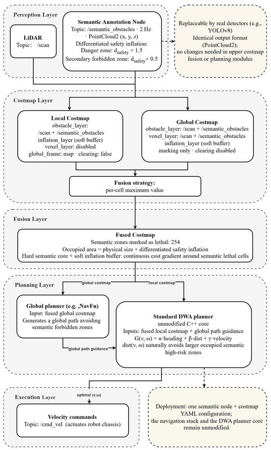
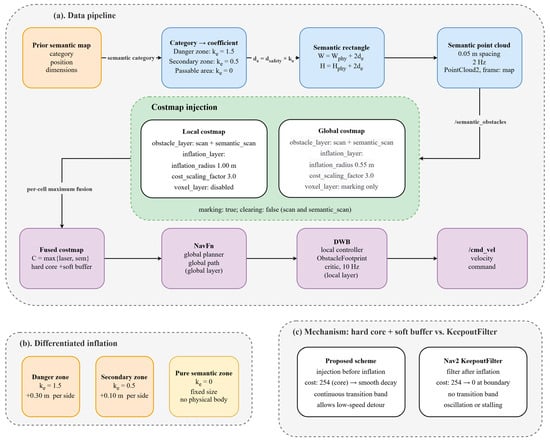
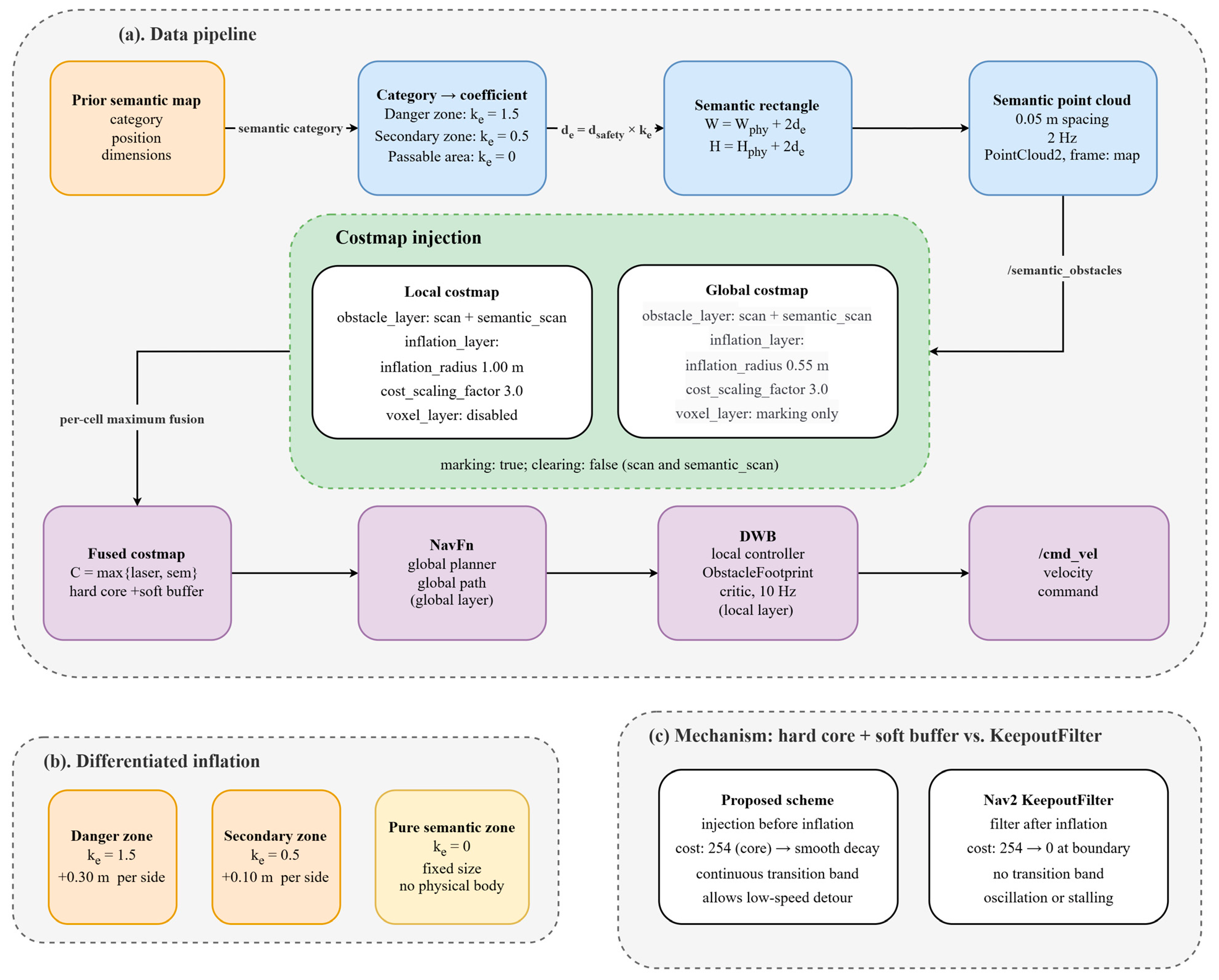
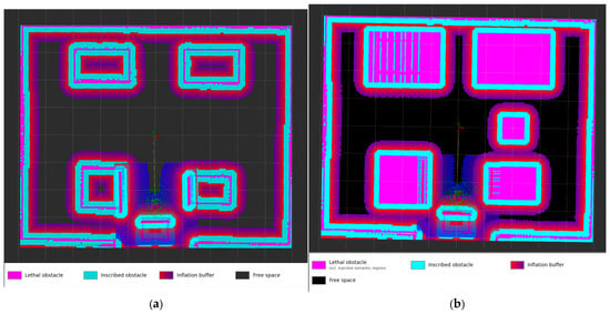
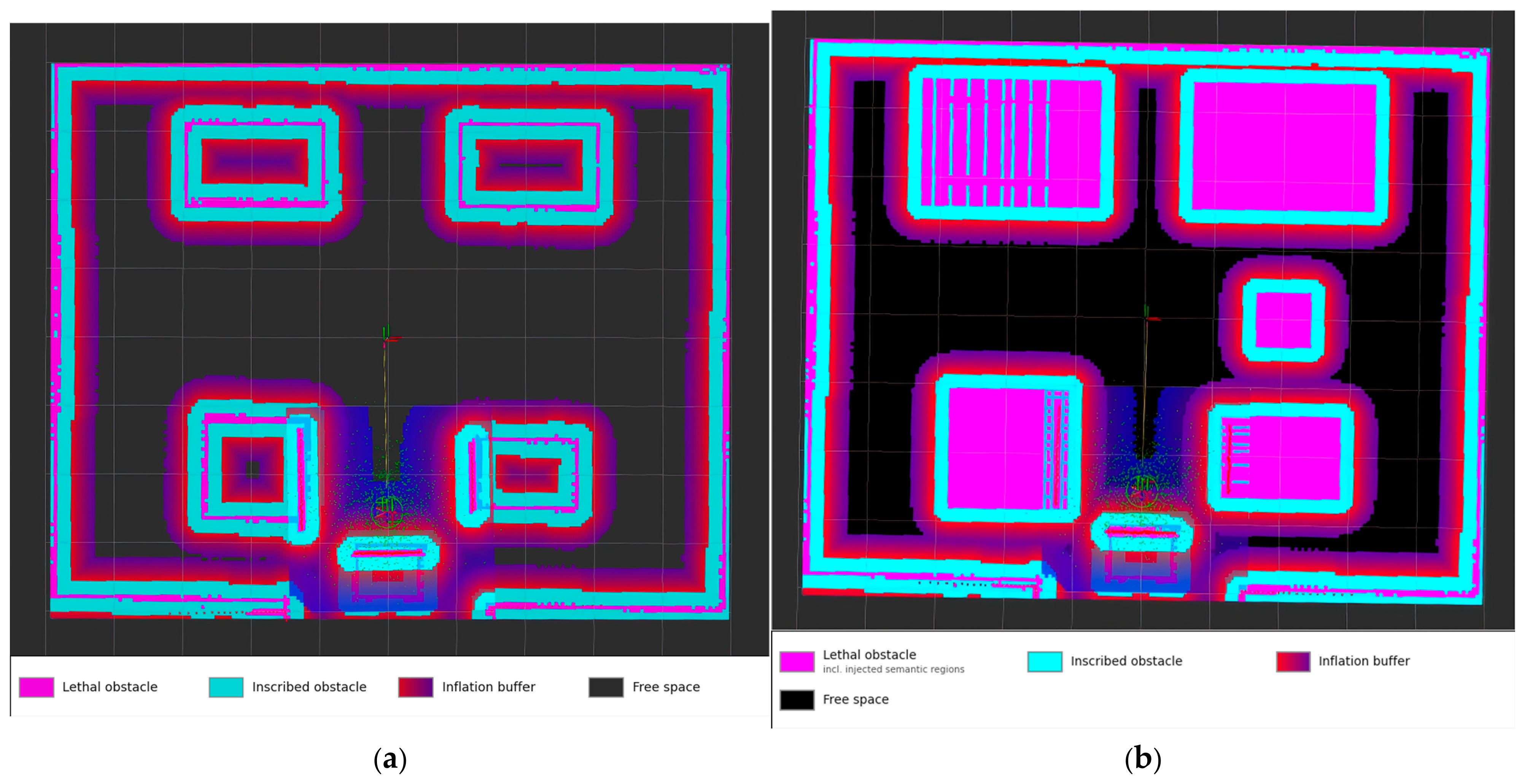
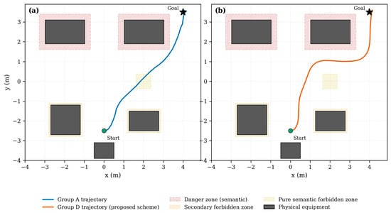
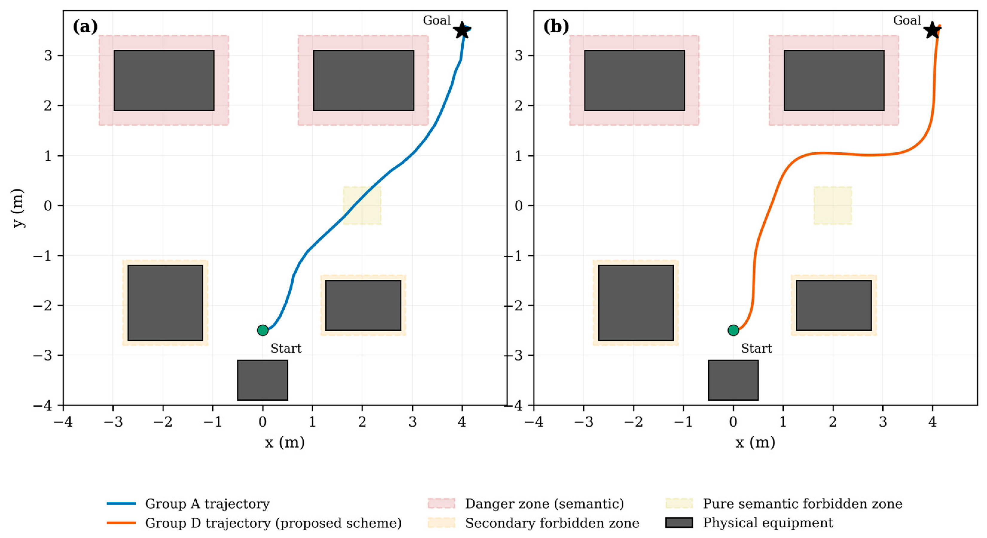
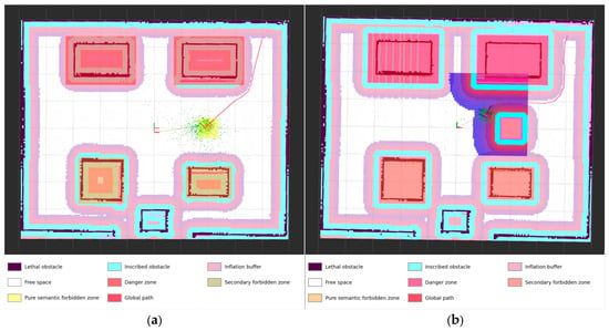
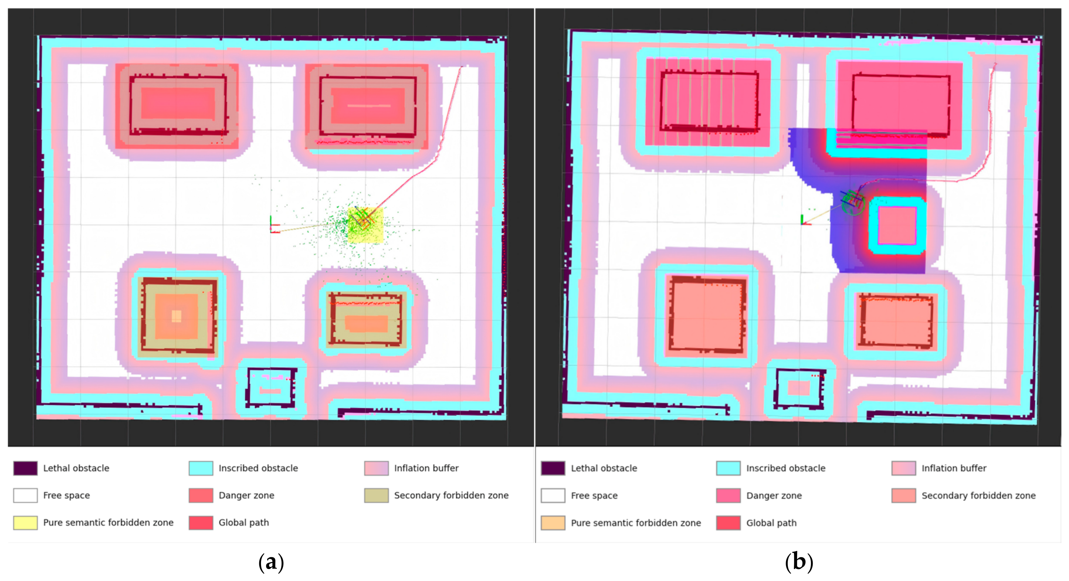
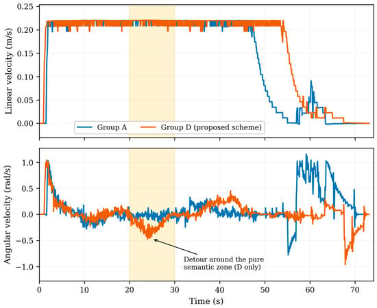
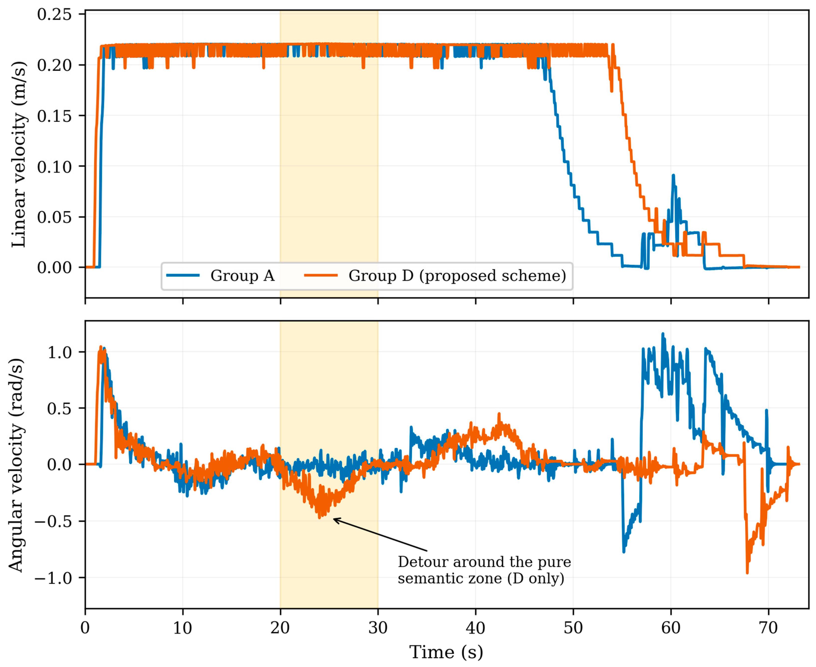
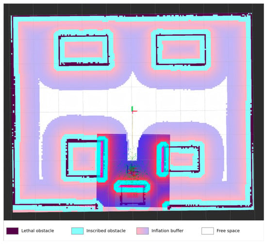
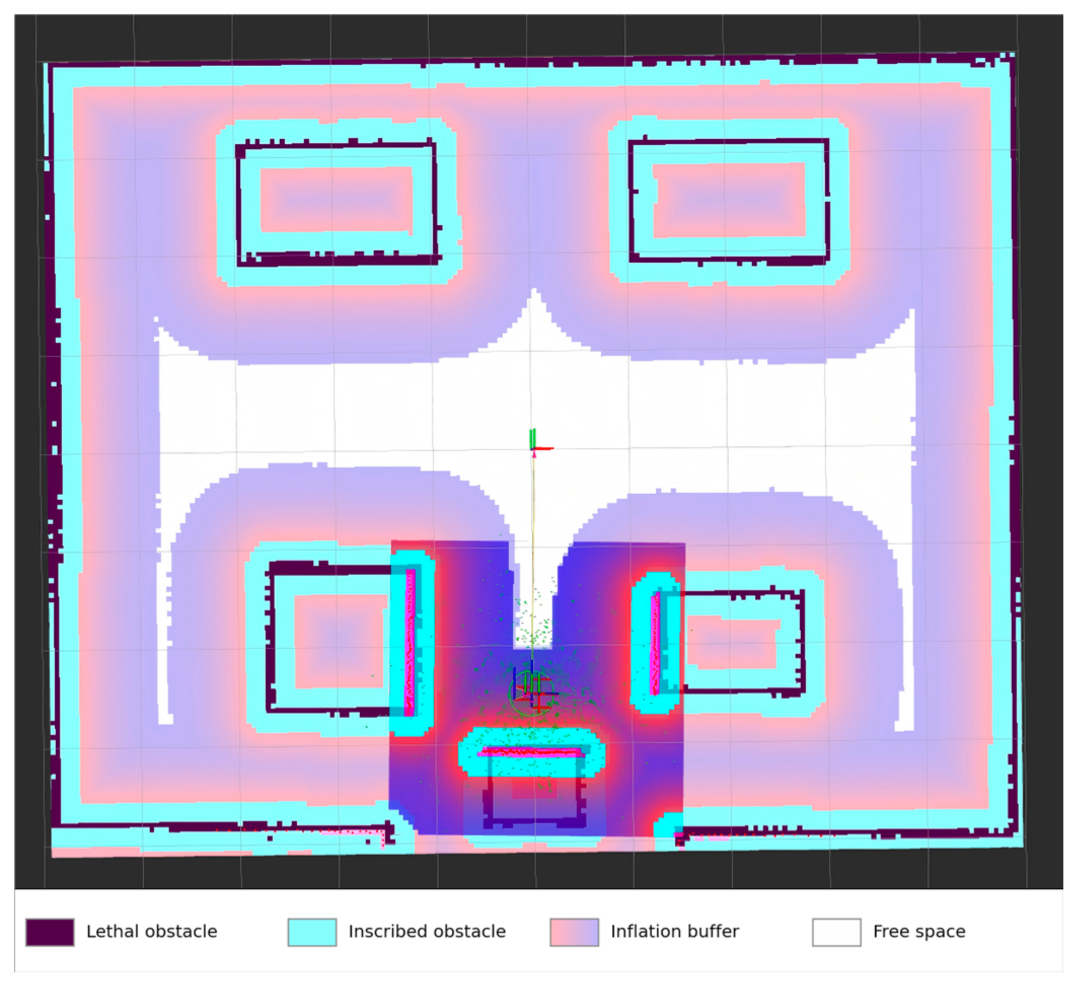
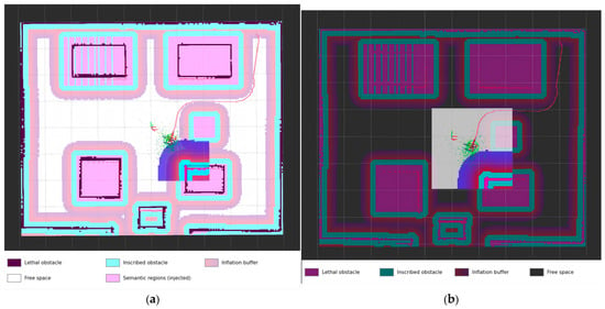
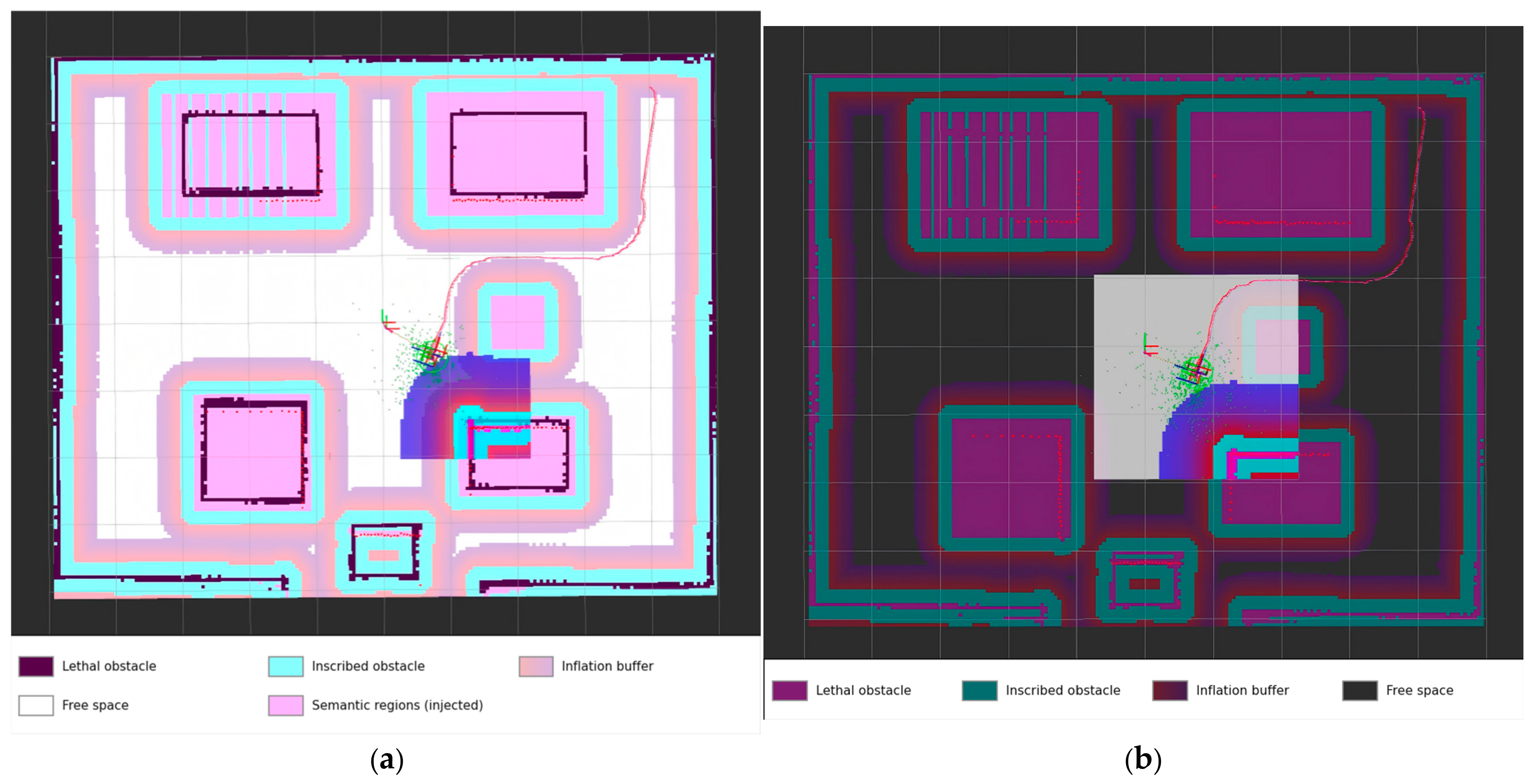
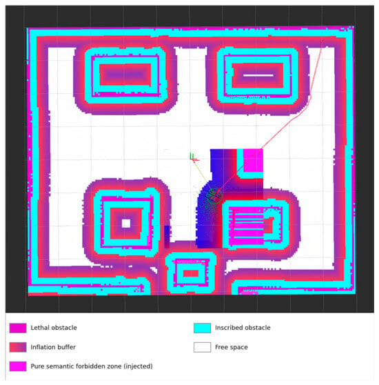
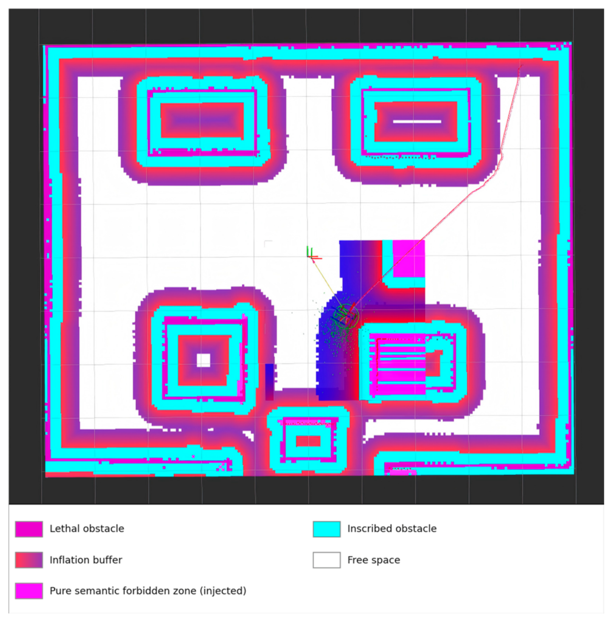
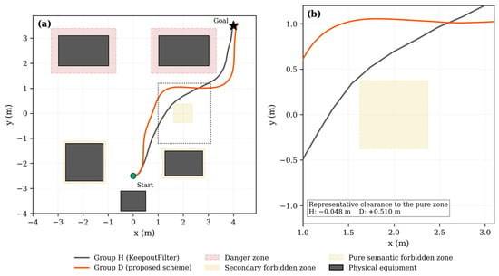
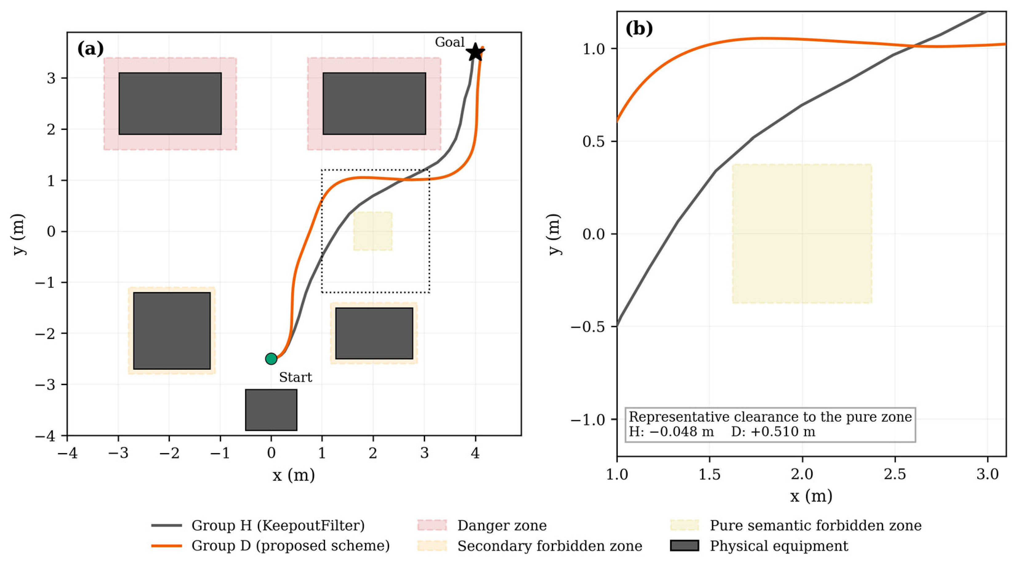
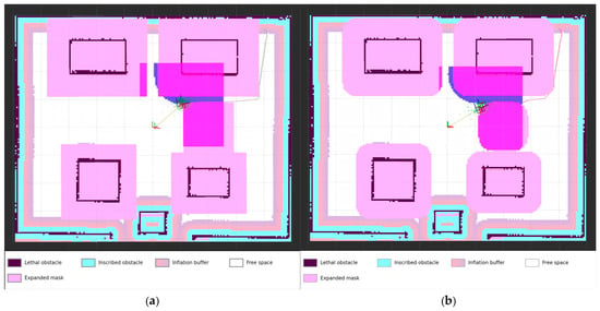
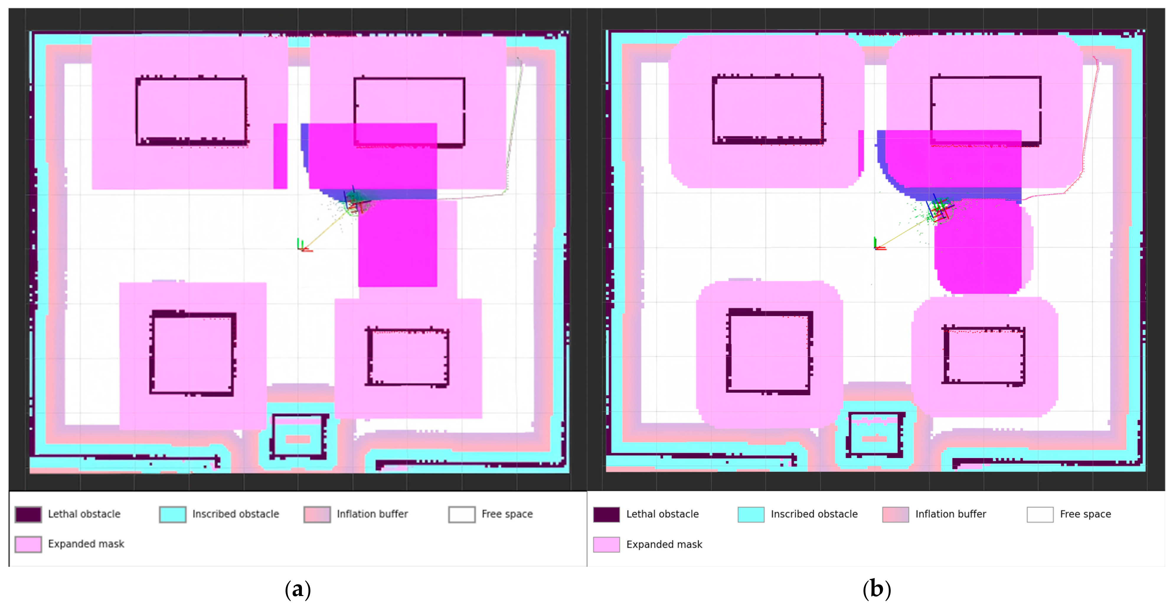
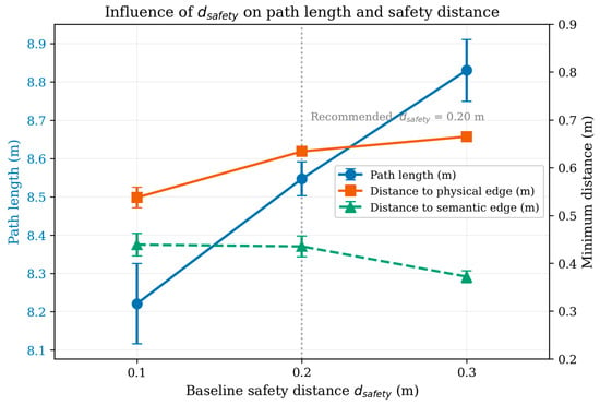
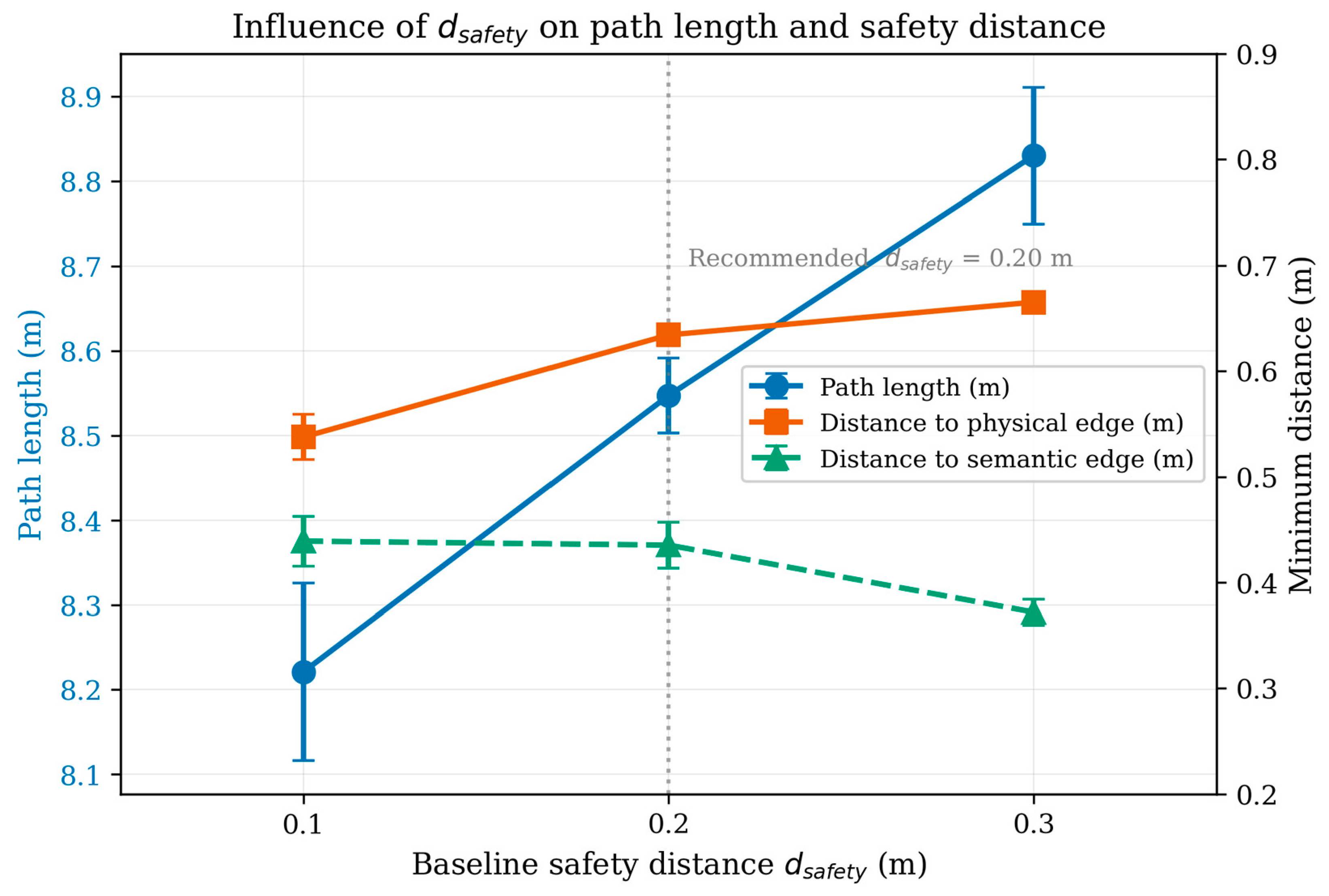
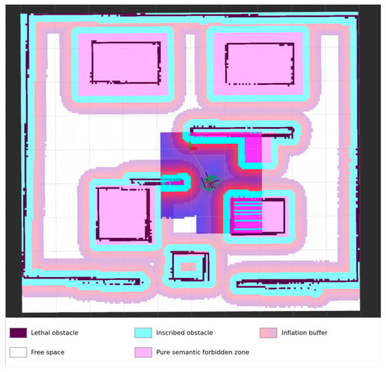
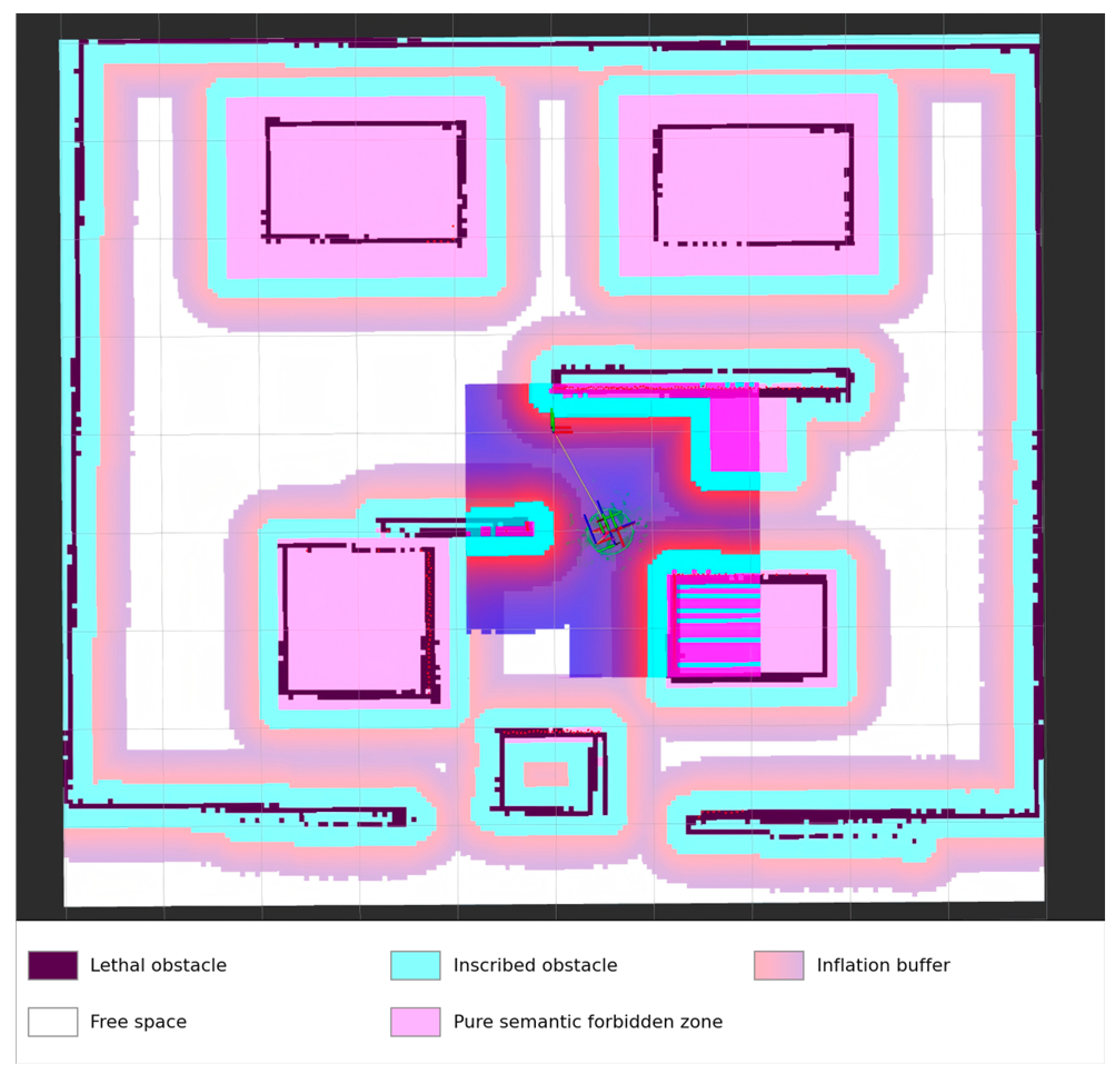

Disclaimer/Publisher’s Note: The statements, opinions and data contained in all publications are solely those of the individual author(s) and contributor(s) and not of MDPI and/or the editor(s). MDPI and/or the editor(s) disclaim responsibility for any injury to people or property resulting from any ideas, methods, instructions or products referred to in the content. |
© 2026 by the authors. Licensee MDPI, Basel, Switzerland. This article is an open access article distributed under the terms and conditions of the Creative Commons Attribution (CC BY) license.