


Abstract
Ultra-fast charging stations can impose substantial short-term power fluctuations and high transformer capacity requirements on distribution networks. To address the coupled planning and operational challenges of such stations, this study proposes a planning-operation coordinated sizing framework for a photovoltaic-integrated ultra-fast charging station. Unlike many existing approaches that address transformer sizing, energy storage configuration, and battery degradation separately or only partially couple them, the proposed framework jointly determines transformer capacity, battery capacity, and supercapacitor capacity while incorporating battery cycling degradation into the long-term storage cost evaluation. Representative charging scenarios are extracted from historical charging-load data and used for capacity planning. At the planning level, the average daily comprehensive cost is minimized by coordinating transformer investment, hybrid energy storage investment, operating cost, and degradation-dependent battery lifetime. At the operation level, battery and supercapacitor dispatch is optimized considering both operating economy and grid-connected power fluctuation. The upper-level sizing problem is solved using quantum-behaved particle swarm optimization. Sobol-sequence initialization and a nonlinear contraction-expansion coefficient are adopted in the implementation to enhance the distribution of the initial population and adjust the search range during the iterative process. The lower-level mixed-integer linear programming problem is solved using Gurobi. In the studied commercial-area case, the proposed hybrid energy storage configuration reduces the transformer capacity from 326 kVA to 201 kVA. Compared with the no-storage scheme, total costs are reduced by 14.9% and 14.3%, while the absolute deviations of grid-connected power are reduced by 93.4% and 94.8% for the two representative days. Compared with battery-only storage, daily battery cycle counts are further reduced by 60.5% and 65.2%. The results demonstrate that the proposed coordinated sizing framework can simultaneously reduce infrastructure capacity requirements and operating costs, improve grid integration performance, and alleviate battery cycling degradation in PV-integrated ultra-fast charging stations.
1. Introduction
With the increasing penetration of electric vehicles, charging infrastructure is developing toward higher charging power and shorter charging duration [1,2]. Ultra-fast charging stations are characterized by high power demand, rapid load variation, and concentrated load peaks, which may increase transformer capacity requirements, intensify grid-power fluctuations, and raise the risk of local overload. Meanwhile, the integration of photovoltaic generation and energy storage provides an effective means of improving renewable energy utilization and alleviating the operational pressure on distribution networks [3]. Therefore, coordinated planning of transformer capacity and energy storage is important for improving both the economy and grid friendliness of PV-storage ultra-fast charging stations.
Existing studies on charging-station planning mainly involve charging-load characterization, energy storage sizing, and optimal dispatch. Representative charging scenarios can be obtained either through probabilistic modeling of user behavior [4,5,6,7] or clustering of historical charging data [8,9,10]. In this study, clustering is used only to generate representative input scenarios for the subsequent capacity-planning model. Regarding capacity planning, existing studies have investigated energy storage sizing and distribution-equipment configuration. However, storage capacity is often optimized independently of transformer capacity [11,12], while other studies mainly consider a single type of storage and therefore cannot fully utilize the complementary power and energy characteristics of hybrid energy storage [13,14]. In addition, treating battery lifetime as a fixed parameter may underestimate the long-term economic impact of frequent cycling under highly fluctuating ultra-fast charging loads [15,16].
In addition, transformer sizing, hybrid energy storage sizing, and short-term operational dispatch are inherently coupled. Transformer capacity determines the power supply capability of the station, whereas the capacity and operating strategy of the energy storage system affect both transformer utilization and grid-connected power fluctuations. Therefore, planning and operation should be coordinated rather than treated as independent optimization problems. Bi-level optimization frameworks have been adopted in previous studies to coordinate planning-level capacity decisions with operation-level scheduling and to balance investment cost, operating cost, and system performance [17,18,19]. Nevertheless, for PV-integrated ultra-fast charging stations, the coordinated effects of transformer sizing, battery-supercapacitor hybrid storage sizing, battery cycling degradation, and grid-oriented dispatch still need to be considered within a unified planning-operation framework.
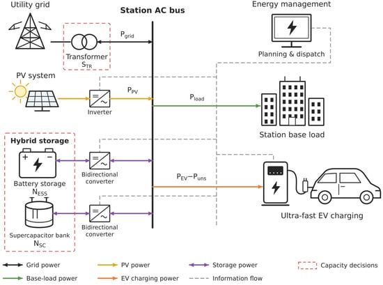
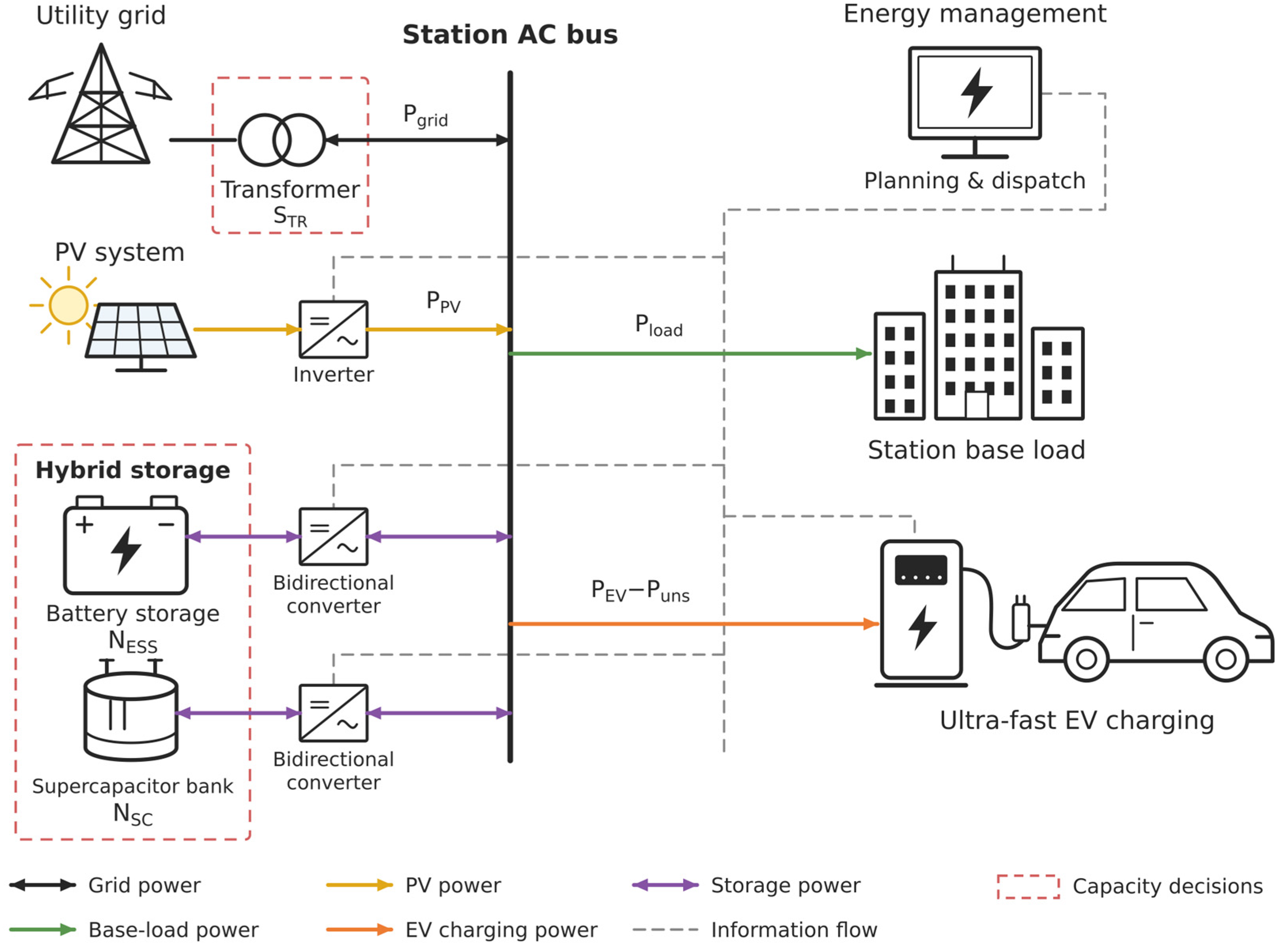
To address the above gaps, this paper develops a bi-level coordinated sizing framework for a commercial-area PV-storage ultra-fast charging station. At the planning level, transformer capacity, battery capacity, and supercapacitor capacity are jointly optimized by minimizing the average daily comprehensive cost, with battery cycling degradation incorporated into the long-term storage cost. At the operation level, battery and supercapacitor dispatch is optimized considering both operating cost and grid-connected power fluctuation. Representative charging scenarios extracted from historical data are used for model evaluation, and no-storage, battery-only, and battery–supercapacitor configurations are compared to quantify their effects on transformer capacity, system economy, grid-power fluctuation, and battery cycling burden. Figure 1 illustrates the system architecture and the power and information flows of the studied PV-integrated ultra-fast charging station. Table 1 summarizes the research aspects discussed above and highlights their joint consideration within the proposed planning–operation framework.
Figure 1.
System architecture and power and information flows of the PV-integrated ultra-fast EV charging station.
Table 1.
Comparison of different studies.
2. Cost Modeling of Transformer and Hybrid Energy Storage
To quantify the economic influence of transformer and hybrid energy storage configuration, this paper first develops cost models for the transformer, supercapacitor, and battery energy storage system. Battery life degradation cost is further considered to provide the objective-function basis for the subsequent optimal configuration and dispatch analysis.
2.1. Transformer Cost Modeling
Reducing the maximum demand of the charging-station transformer can lower investment cost, but during load peaks, some users may be unable to charge normally. This not only causes electricity-sales revenue loss but also affects user satisfaction. So this paper imposes a hard transformer capacity constraint and includes an economic penalty for unserved EV charging energy in the objective function [20]. The charging energy that cannot be supplied is multiplied by a penalty factor and included in the objective function. When limited transformer capacity prevents user charging, the corresponding lost energy is amplified by the penalty factor and reflected in the optimization model.
2.1.1. Transformer Penalty Cost
The penalty cost is derived from the charging-energy loss cost Clos caused by the limited configured transformer capacity. When EV charging demand cannot be fully supplied by the grid, photovoltaic generation, and energy storage within the transformer capacity limit, the unmet portion is represented by the unserved charging power . This portion of demand is discarded rather than postponed or supplied in a later interval.
where α is the penalty factor for unserved EV charging energy; Cj is the grid electricity price in period j, in CNY/kWh; is the unserved EV charging power in period j, in kW; is the requested EV charging power in period j, in kW; STR is the configured transformer capacity, in kVA; PTRS is the maximum allowable active power through the transformer in kW; and k is the assumed fixed power factor. The unmet portion of charging demand is discarded rather than supplied in a later interval and is subtracted from the requested EV load in the power-balance equation.
PTRS = k ⋅ STR,
2.1.2. Transformer Investment Cost
The transformer investment cost CTRS′ consists of two parts: the annualized investment cost C1 and the basic capacity charge C2:
where b1 is the depreciation rate; n1 is the operating lifetime of the transformer; CT is the unit transformer capacity price, in CNY/kVA; and A is the basic transformer capacity charge, which is 28 CNY/(kVA·month).
CTRS′ = C1 + C2,
C2 = 12A ⋅ STR,
2.2. Supercapacitor Cost Modeling
The cost of the supercapacitor considered in this paper mainly consists of operation and maintenance cost and initial investment cost. The operation and maintenance cost reflects the consumption and maintenance expenditure during daily charging and discharging, while the investment cost represents the fixed expenditure of the energy storage device over its full life cycle. Since the cycle life of supercapacitors is much longer than that of lithium-ion batteries and their life degradation is relatively small [21], the cycle-life degradation of the supercapacitor is not considered in this paper, and its lifetime is treated as a fixed value.
2.2.1. Supercapacitor Operation and Maintenance Cost Com,SC
The operation and maintenance cost of the supercapacitor is calculated by multiplying its charging and discharging energy throughput by the unit energy-throughput O&M cost coefficient:
where is the supercapacitor O&M cost coefficient, in CNY/kWh; is the charging power of the supercapacitor in period j; and is the discharging power of the supercapacitor in period j.
2.2.2. Supercapacitor Investment Cost Cinvs,SC
2.3. Battery Cost Modeling
The cost of the battery energy storage system also consists of operation and maintenance cost and investment cost. The operation and maintenance cost reflects energy loss and maintenance expenditure during daily charging and discharging, and its calculation is consistent with that of the supercapacitor. The investment cost represents the initial expenditure of the battery energy storage system over its life cycle. Since battery life degradation occurs during cyclic operation, the lifetime parameter n2 is no longer treated as a fixed value, but is dynamically determined according to the actual depth of charge and discharge and the number of cycles.
2.3.1. Battery Energy Storage Operation and Maintenance Cost Com,ESS
Similarly, the battery operation and maintenance cost is calculated by multiplying its total charging and discharging energy throughput by the corresponding unit energy-throughput O&M cost coefficient:
where is the battery O&M cost coefficient, in CNY/kWh; is the charging power of the battery energy storage system in period j; and is the discharging power of the battery energy storage system in period j.
2.3.2. Battery Energy Storage Investment Cost Cinvs,ESS
The calculation is consistent with that of the supercapacitor, but the battery lifetime n2 is not treated as a constant.
where is the unit price of the battery energy storage system, in CNY/kWh; NESS is the number of configured battery energy storage units; EESS,R is the rated energy capacity of a single battery energy storage unit, in kWh/unit; n2 is the service life of the battery; and b2 is the depreciation rate.
2.4. Battery Life Degradation Modeling
In practical operation, battery life is affected by multiple factors, including temperature, depth of discharge, cycle count, and charge–discharge rate [22].
Since this study primarily investigates the influence of dispatch strategies on life-cycle cost, battery degradation is evaluated using DOD-dependent cycle life and rainflow cycle counting to balance model detail and computational complexity. The same cycle-life relationship under the reference conditions of the underlying data is applied to all configurations. Temperature-dependent degradation, calendar aging, and the additional influence of charge–discharge rate are not explicitly modeled. Although charge–discharge rate varies with the dispatch strategy, its effect on degradation is not separately quantified in the present model. The calculated lifetime should be interpreted as a cycle-limited estimate under the adopted assumptions.
The relationship between cycle life and depth of discharge differs among battery types. In this paper, lithium iron phosphate batteries are selected for the energy storage configuration. Table 2 lists the cycle-life data of the selected lithium iron phosphate battery under different depths of discharge [23].
Table 2.
Battery Cycle Life Versus Depth of Discharge.
Based on the data in the table, the relationship between battery cycle count and depth of discharge can be fitted by a third-order polynomial function:
where d is the battery depth of discharge, and N is the battery cycle life corresponding to depth of discharge d.
N(d) = −2083d3 + 8750d2 − 13170d + 11200,
In actual operation, the battery experiences irregular charging and discharging patterns with cycles of different depths. Rainflow counting is therefore applied to the battery state-of-charge (SOC) trajectory to identify these cycles [24]. The input includes the initial SOC and the SOC at the end of every dispatch interval. For each identified cycle i, the SOC range defines its DOD, di, and the associated cycle count, ci, is 1 for a full cycle and 0.5 for a residual half-cycle. Zero-range events are excluded. Constant-SOC intervals do not introduce additional reversals, so they do not split a discharge excursion into separate cycles.
For a complete cycle with depth of discharge d, the conversion coefficient K for equivalent cycles at 100% depth of discharge is defined as:
where N(1) is the cycle count of the battery at 100% depth of discharge. Substituting d = 1 into the fitted cycle-life relationship gives N(1) ≈ 4700.
K(d) = N(1)/N(d),
The daily damage-equivalent cycle count for representative day s is then calculated as:
where Ms is the number of nonzero-range rainflow entries for representative day s.
For multiple representative days, the average daily damage-equivalent cycle count is obtained using their occurrence weights. The corresponding cycle-limited battery lifetime is:
where Teq is the equivalent battery lifetime in years, and the calculated value is used as the battery service life n2 in Section 2.3; Ns is the number of representative days; ws is the fraction of annual days represented by day s. For a single representative day, ws is set to 1. The weights are obtained from the cluster proportions described in Section 5.1. Annual lifetime estimation assumes that these proportions remain representative throughout the year.
2.5. Photovoltaic Cost Modeling
The PV capacity and generation profiles are prescribed inputs rather than sizing decision variables in this study. But PV operation and maintenance expenditure is included in the system operating cost. The daily PV operation and maintenance cost is calculated by multiplying the daily PV generation by a unit energy-based O&M cost coefficient:
where is the PV operation and maintenance cost coefficient, in CNY/kWh; is the PV generation power in dispatch interval j, in kW.
3. Construction of the Bi-Level Optimization Model
Charging-station loads are characterized by large fluctuations and short-duration peaks. If transformers and energy storage systems are configured directly according to the maximum load, equipment utilization may be low and economic performance may be poor. Therefore, this paper constructs a bi-level optimal configuration model containing a planning layer and an operating layer. The upper layer performs capacity configuration by minimizing the average daily comprehensive cost, while the lower layer performs optimized dispatch by minimizing daily operating cost and grid-connected power fluctuation.
3.1. Upper-Layer Optimal Configuration
3.1.1. Optimal Configuration Objective
The energy storage optimal configuration model takes the minimization of the average daily comprehensive system cost as the optimization objective. The average daily comprehensive system cost mainly consists of system operating cost and system investment cost. For ease of understanding, the following analyses are presented on a single representative-day basis. The overall objective function is calculated as the weighted sum of the representative-day objective values, using occurrence weights derived from the clustering results.
f1 = min(Cyx + Cinvs),
The system operating cost Cyx includes grid electricity purchase cost, grid electricity sales revenue, hybrid energy storage operation and maintenance cost, transformer penalty cost and PV operation and maintenance cost.
where:
Cyx = Cbuy − Csell + Com + Clos + Com,PV,
Grid electricity purchase cost Cbuy.
The grid electricity purchase cost is obtained by summing the product of grid purchase power and the corresponding electricity purchase price over all periods.
where denotes the power purchased from the grid in period j, and Cj is the time-of-use electricity price in period j.
Grid electricity sales revenue Csell.
The grid electricity sales revenue is obtained by summing the product of grid electricity sales power and the corresponding selling price over all periods.
where denotes the power sold to the grid in period j, and Cs is the electricity selling price. Although the feed-in tariff for distributed photovoltaic generation has gradually shifted from a fixed price to a market-based mechanism [25], the surplus electricity feed-in price is uniformly set to 0.29 CNY/kWh in this paper for ease of analysis.
Hybrid energy storage operation and maintenance cost Com.
The hybrid energy storage operation and maintenance cost includes the operation and maintenance costs of the supercapacitor and the battery energy storage system.
Com = Com,SC + Com,ESS.
The transformer penalty cost Clos is the same as that described in Section 2.1.
The system investment cost Cinvs includes transformer investment cost and hybrid energy storage investment cost.
Cinvs = CTRS + CHESS.
Transformer investment cost CTRS.
CTRS′ in Section 2.1.2 denotes the annual transformer investment cost, which is converted here into the daily cost CTRS:
CTRS = CTRS′/365.
Hybrid energy storage investment cost CHESS.
The hybrid energy storage investment cost includes the investment costs of the supercapacitor and the battery energy storage system.
CHESS = Cinvs,SC + Cinvs,ESS.
3.1.2. Constraints
The energy storage configuration model requires the installed capacities of the energy storage devices to be within specified ranges:
where NESS,min and NESS,max are the lower and upper bounds of the number of battery units, respectively; NSC,min and NSC,max are the lower and upper bounds of the number of supercapacitor units, respectively; and STR,min and STR,max are the lower and upper bounds of the rated transformer capacity, respectively, in kVA.
NESS,min ≤ NESS ≤ NESS,max,
NSC,min ≤ NSC ≤ NSC,max,
STR,min ≤ STR ≤ STR,max,
3.2. Lower-Layer Optimal Dispatch
3.2.1. Optimal Dispatch Objective
The energy storage optimal dispatch model aims to minimize daily operating cost and grid-connected power fluctuation. The daily operating cost is calculated in the same way as in Section 3.1.
According to the system power balance, after the hybrid energy storage system is incorporated, the grid-connected power can be expressed as:
where is the grid-connected power in period j; is the base load within the charging station; and is the photovoltaic power in period j.
To characterize the fluctuation degree of grid-connected power within each hour, the average grid-connected power in hour h is defined as:
where Ωh is the set of dispatch periods corresponding to hour h, and Nh is the number of periods in that hour. In this paper, the dispatch interval is 5 min; therefore, Nh = 12.
The average absolute deviation of grid-connected power in hour h is further defined as:
The full-day grid-connected power fluctuation index is then expressed as:
Therefore, the objective function of the lower-layer optimal dispatch model can be written as:
minf2 = Fgrid + λCyx.
Since different objective functions have different dimensions and numerical scales, dimensionless normalization is performed to avoid the influence of inconsistent units on the optimization results. The normalized objective function is written as:
where is the grid-connected power fluctuation before optimization, and is the operating cost before optimization.
3.2.2. Basic Constraints
First, the system power balance must be satisfied, and the grid-connected power must remain within the transformer’s maximum allowable power limit in both import and export directions:
Second, the charging and discharging power of the hybrid energy storage system must remain within specified ranges:
where PESS,R and PSC,R are the rated powers of a single battery unit and a single supercapacitor unit, respectively.
Then, the state of charge of the hybrid energy storage system must remain within specified ranges:
where , are the lower and upper SOC limits of the battery, respectively; , are the lower and upper SOC limits of the supercapacitor, respectively; is the battery SOC in period j; and is the supercapacitor SOC in period j.
and are calculated using the following two equations:
where ηESS,C, ηESS,D are the charging and discharging efficiencies of the battery, respectively; ηSC,C, ηSC,D are the charging and discharging efficiencies of the supercapacitor, respectively; EESS,R is the rated energy capacity of a single battery unit, in kWh/unit; and ESC,R is the rated energy capacity of a single supercapacitor unit, in kWh/unit.
In addition, cyclic SOC constraints are imposed on both the battery and the supercapacitor. Their initial and terminal SOC values are fixed at 0.5 for each representative day:
these constraints prevent the model from reducing daily operating cost by leaving either storage device with a lower energy level at the end of the day.
Finally, the grid-connected power also needs to be constrained. At present, there is no explicit standard for the grid-connected power fluctuation of charging stations with photovoltaic generation and energy storage. Referring to the grid-connection requirements for photovoltaic power stations [26], the average absolute deviation of grid-connected power within each hour is limited to within 10% of the transformer capacity. On this basis, to avoid an excessively strict constraint that would reduce the feasible region, a tolerance term Ptol is introduced, and the final constraint is written as:
Dgrid,h ≤ 0.1PTRS + Ptol.
3.2.3. Coordination and Allocation Constraints of Hybrid Energy Storage
To reflect the complementarity between battery energy storage and supercapacitors in dynamic response characteristics, this paper adopts a moving-average-based power decomposition method to allocate the output power of the hybrid energy storage system. The net output powers of the battery and supercapacitor are defined as:
To characterize the power fluctuation that needs to be smoothed by the energy storage system, the net load power is defined as:
A moving-average filter [27] is used to extract the low-frequency component , and the high-frequency component is then obtained as:
On this basis, the supercapacitor preferentially undertakes the high-frequency fluctuation component of the net load, while the battery mainly undertakes the low-frequency smoothing power. In addition, to suppress frequent and rapid battery regulation, the variation in the battery net output power between adjacent periods is constrained as:
where γ is the ramping coefficient and Pbat = NESSPESS,R.
Through the above constraints, the supercapacitor is encouraged to preferentially undertake high-frequency fluctuation components, while the battery mainly undertakes low-frequency smoothing power.
The auxiliary variables and linear constraints used to reformulate the absolute-value expressions, together with the binary constraints preventing simultaneous charging and discharging, are provided in Appendix B. And a comparison of the convergence performance of improved QPSO, standard QPSO, and PSO over 10 independent runs is presented in Appendix C.
4. Solution Strategy
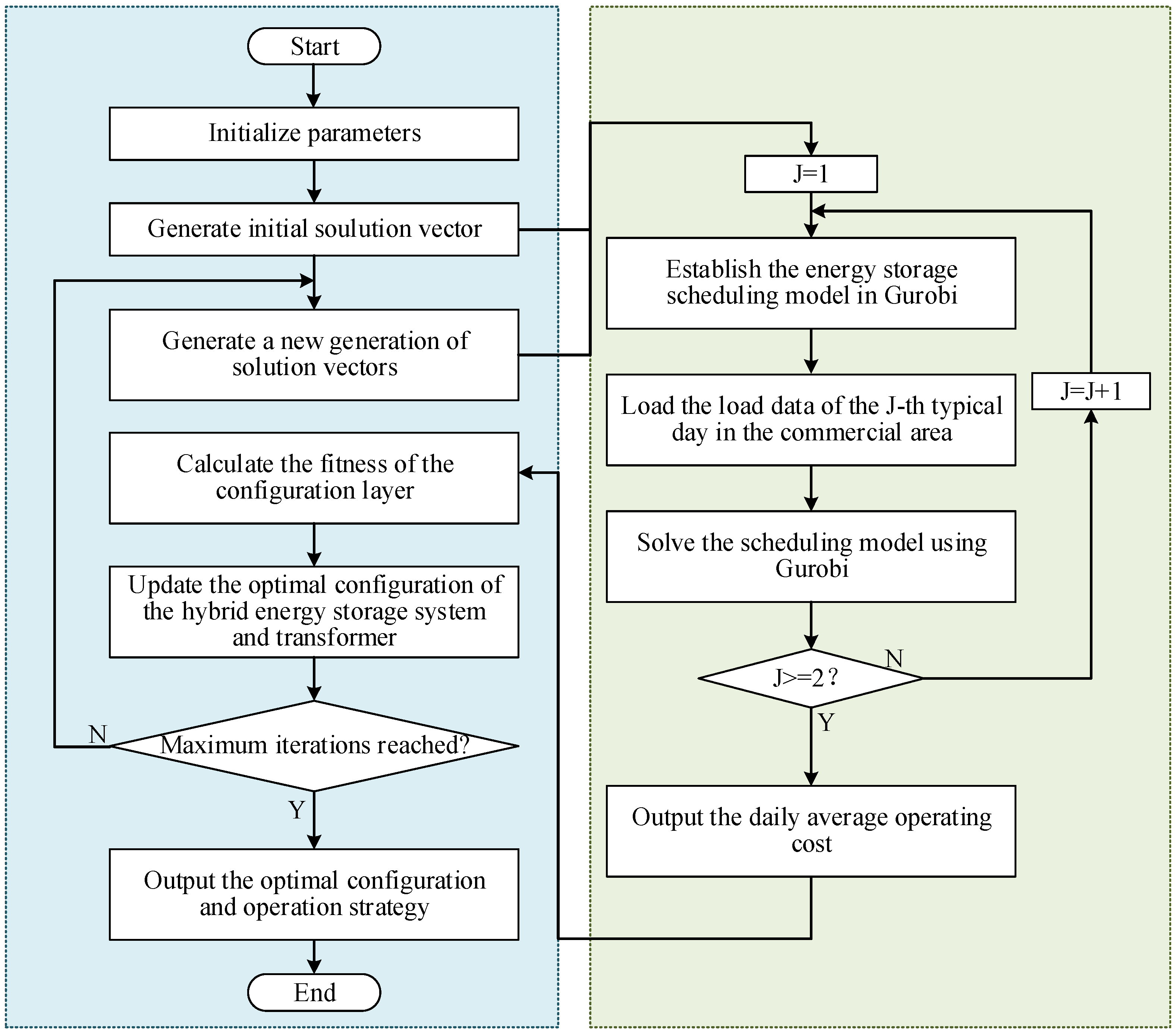
The proposed bi-level model is solved using a nested solution strategy. The upper-level sizing problem jointly determines the transformer, battery, and supercapacitor capacities using an improved quantum-behaved particle swarm optimization (QPSO) algorithm, while the lower-level mixed-integer linear programming (MILP) problem is solved using Gurobi 10.0.3. To improve the initial population coverage and balance global exploration and local exploitation, Sobol-sequence initialization and a nonlinear contraction-expansion coefficient are introduced into the standard QPSO. The detailed QPSO formulation, parameter settings, stopping criteria, and procedures for integer rounding and constraint handling are provided in Appendix A.
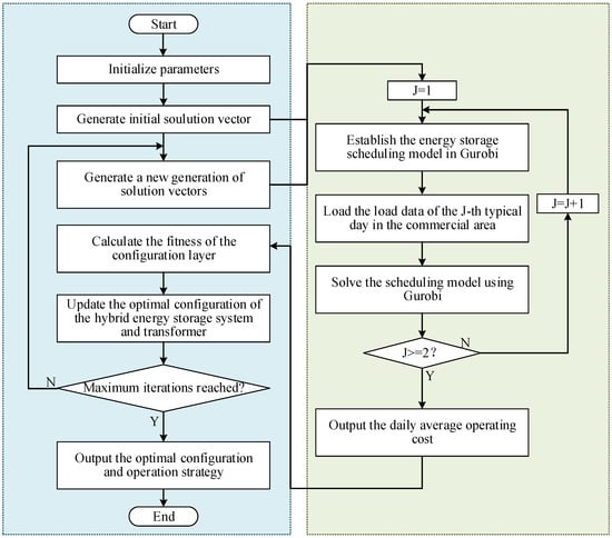
During each upper-level iteration, QPSO generates candidate values of transformer capacity, battery capacity, and supercapacitor capacity. For each candidate configuration, the lower-level MILP determines the optimal daily dispatch of the battery and supercapacitor subject to the operational constraints described in Section 3. The resulting operating cost and grid-power fluctuation index are returned to the upper level for fitness evaluation. This procedure is repeated until the prescribed stopping criterion is satisfied. The overall solution procedure is shown in Figure 2.
Figure 2.
Solution flowchart of the bi-level optimization model.
5. Case Study
5.1. Basic Case-Study Data
In this case study, charging load data from a conventional charging station in a commercial area of Anhui Province, China, are used as the basis for constructing a PV-storage ultra-fast charging station scenario. Charging demand in the commercial-area scenario is concentrated and fluctuates significantly, which can effectively reflect the role of the energy storage system in smoothing fluctuations and improving economic performance.
The base-load and EV charging-demand profiles have a temporal resolution of 15 min, with 96 intervals per day. To match the 5 min dispatch interval, each 15 min power value is held constant over three consecutive 5 min intervals, yielding 288 intervals per day while preserving the daily energy of each profile. The PV generation profiles are supplied as 288 power values per day and used directly at the 5 min dispatch resolution.
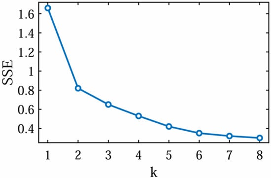
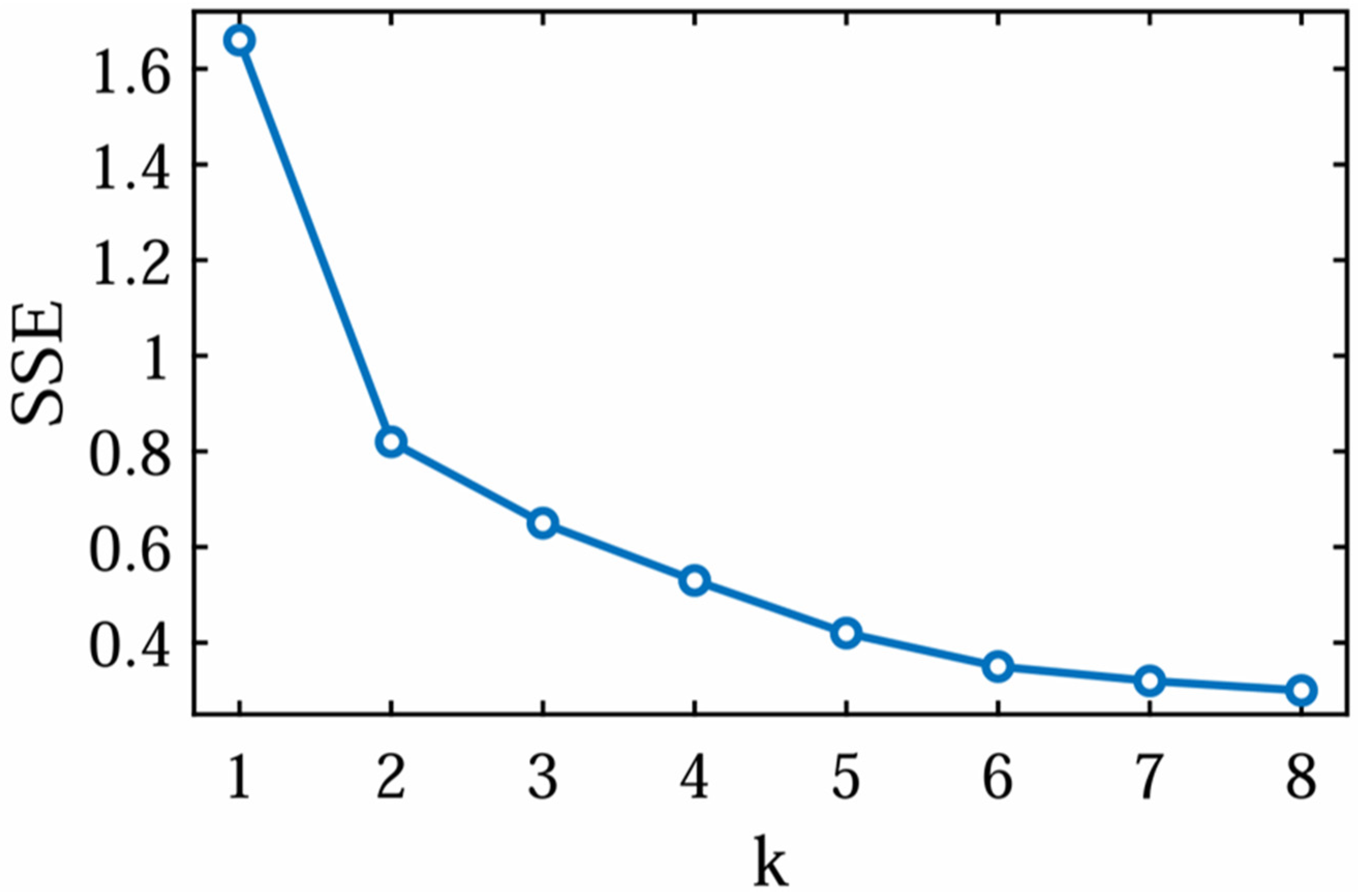
Based on historical charging-load data from August and September, K-means clustering is used to process the daily charging-load curves [28]. The SSE curves corresponding to different numbers of clusters are shown in Figure 3. As shown in Figure 3, SSE decreases most significantly when the number of clusters increases from 1 to 2, while the decrease becomes gradual thereafter.
Figure 3.
SSE curve.
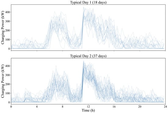
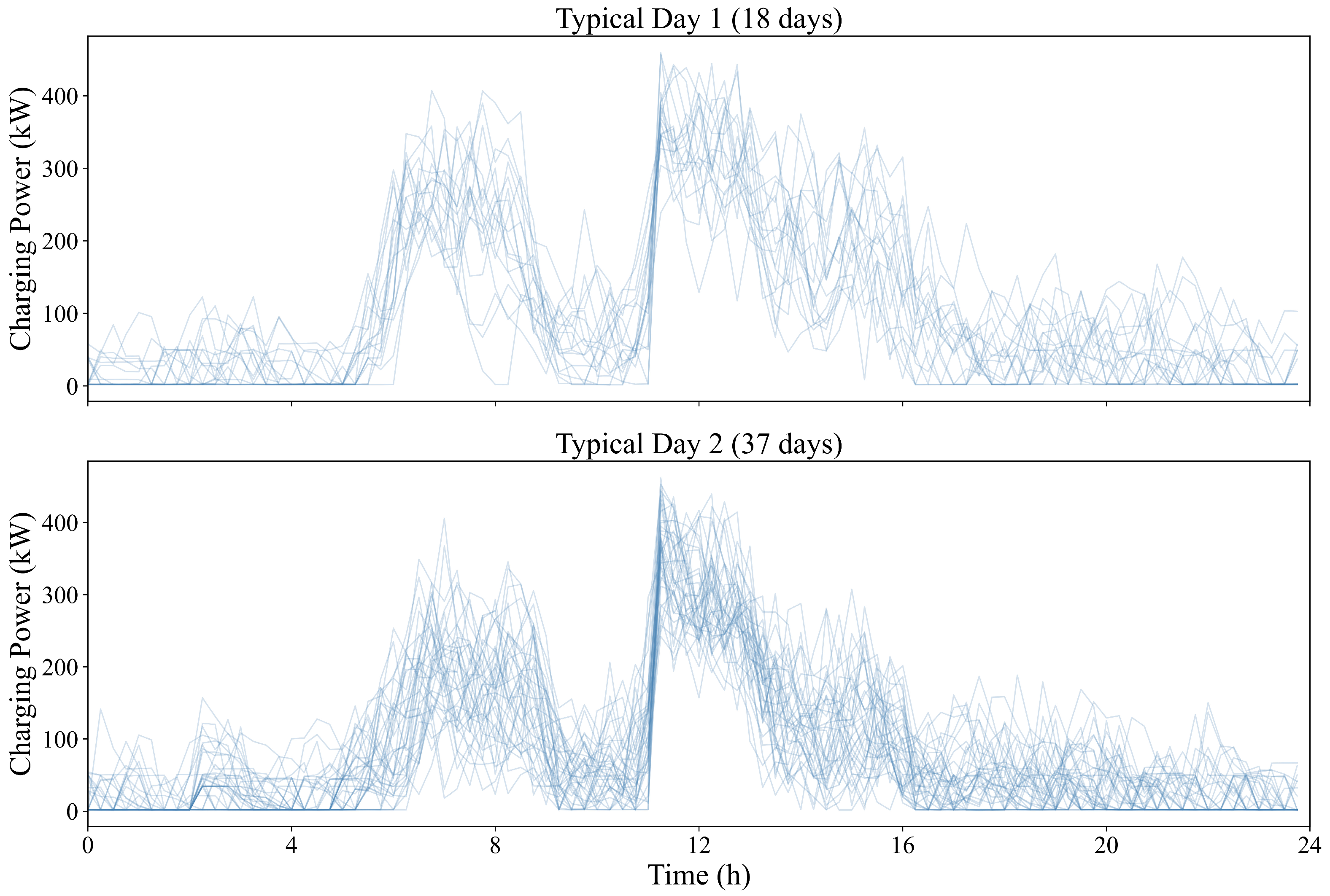
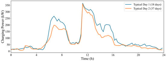
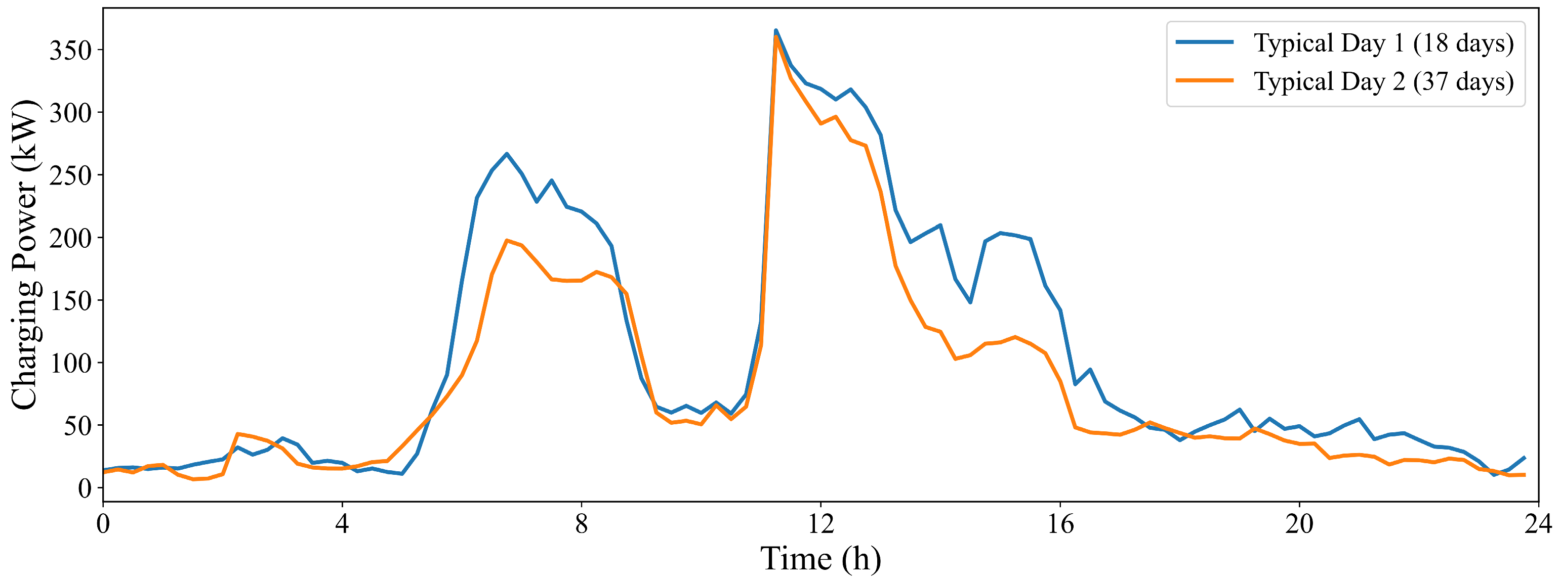
According to the elbow method, the charging load in the commercial-area scenario is divided into two typical days, and the results are shown in Figure 4 and Figure 5. On this basis, the two typical-day loads are used as inputs to the bi-level optimization model, together with time-of-use electricity prices, photovoltaic output, and equipment parameters, to further analyze the system configuration and dispatch performance.
Figure 4.
Load categories and proportions in the commercial-area scenario.
Figure 5.
Clustering results in the commercial-area scenario.
Each daily charging-load curve is treated as an individual sample in the clustering process. The clusters corresponding to typical days 1 and 2 contain 18 and 37 daily samples, respectively. Their weights are therefore calculated as w1 = 18/(18 + 37) and w2 = 37/(18 + 37). These weights represent the observed proportions within the historical dataset and are used to aggregate the representative-day results.
As shown in Figure 4 and Figure 5, the two typical-day loads in the commercial-area scenario both exhibit low nighttime levels and significant increases during the daytime, with the daily peak occurring at around 11:00. This indicates that charging demand is mainly concentrated in daytime periods. In comparison, the load level of typical day 1 is generally higher than that of typical day 2 in the morning and afternoon periods, and the high-load duration is longer. Typical day 2 drops more rapidly after the noon peak and has a relatively smoother load profile throughout the day. The two typical days effectively reflect the differences in peak level and duration of commercial-area charging loads, providing representative inputs for the subsequent optimization analysis.
The grid purchase price adopts a time-of-use tariff. Different electricity prices are applied in different periods, guiding the energy storage system to charge at low prices and discharge at high prices, thereby affecting capacity configuration and dispatch behavior. The specific tariff parameters are listed in Table 3.
Table 3.
Time-of-use electricity price table.
For energy storage system parameters, this paper considers a hybrid energy storage system composed of batteries and supercapacitors. The battery energy storage system mainly undertakes peak shaving, valley filling, and low-frequency regulation, while the supercapacitor is mainly used to suppress short-term fluctuations and reduce battery life degradation. The related parameters, including rated capacity, charging/discharging efficiency, and state-of-charge constraints, are listed in Table 4.
Table 4.
Parameters of batteries and supercapacitors.
The remaining system parameters, including power factor, sizing bounds, penalty coefficient, fluctuation tolerance, battery ramping coefficient, and objective weighting factor, are summarized in Table 5.
Table 5.
System model and economic parameters.
Based on the above data and parameter settings, three schemes are compared in this paper: no energy storage, battery-only energy storage, and battery-supercapacitor hybrid energy storage. The differences in operating cost and power fluctuation suppression under different configuration schemes are then analyzed.
5.2. Upper-Layer Optimal Configuration Results
In the commercial-area scenario, the two typical-day loads, photovoltaic output, and time-of-use electricity prices are input into the upper-layer optimal configuration model. Three schemes are compared: no energy storage, battery energy storage, and battery-supercapacitor hybrid energy storage. The no-storage scheme is used as the benchmark and does not involve capacity optimization. The other two schemes jointly optimize energy storage capacity and transformer capacity while satisfying system operating constraints. The results are listed in Table 6.
Table 6.
Upper-layer configuration results.
It needs to be explained that the supercapacitor unit count in Table 5 refers to individual cells. With a cell capacitance of 3000 F and a rated voltage of 2.7 V, the rated stored energy of each cell is ESC,R = 0.5·CV2/(3.6 × 106) ≈ 0.00304 kWh. The configuration of 4299 cells therefore corresponds to approximately 13.1 kWh of total rated stored energy. Within the adopted energy-based SOC range of 0.1–0.9, the usable stored energy is approximately 10.45 kWh.
The cell power parameter of approximately 6.28 kW is calculated from V2/(4 R), using an ESR of 0.29 mΩ. This parameter represents theoretical impedance-match power rather than a continuous operating rating. Its aggregate value of approximately 27 MW consequently does not represent the continuous power available at the station interface. Dispatch is additionally restricted by the SOC dynamics and available energy. Specifically, the discharge constraint implies
For a 5 min interval and a discharge efficiency of 0.95, the maximum average discharge-power bound obtained from the full allowable SOC range is approximately 119.1 kW; the available bound is lower when the starting SOC is below its upper limit.
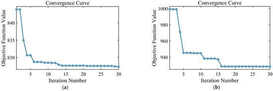
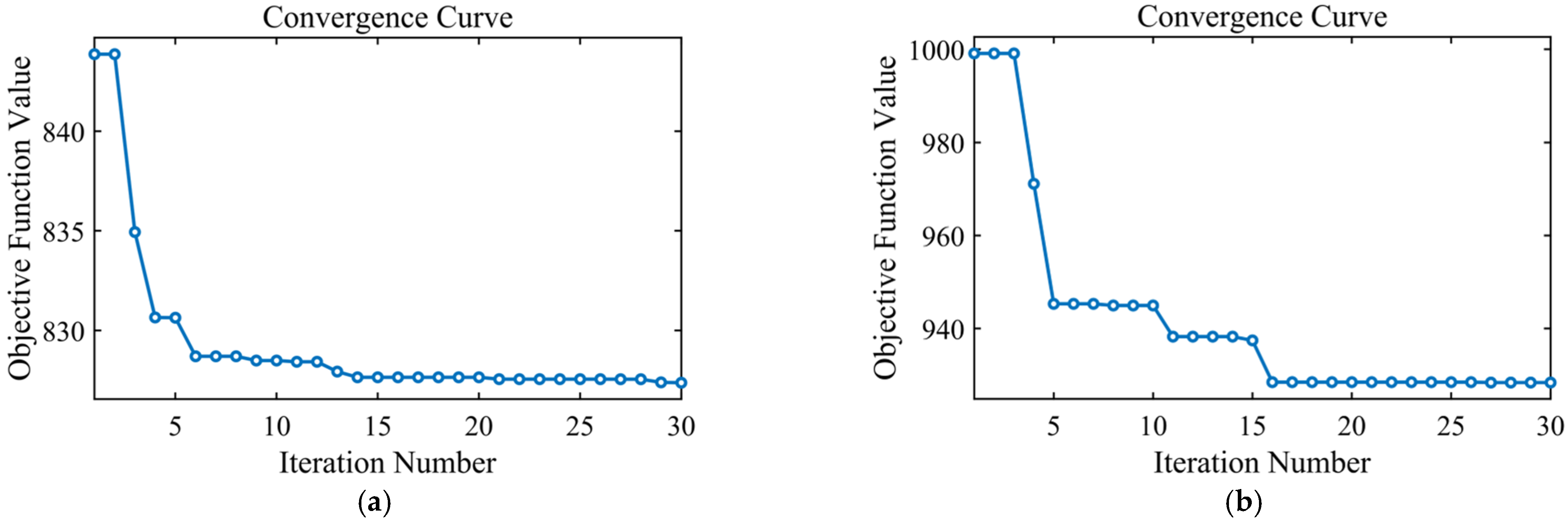
The iterative process of the upper-layer algorithm is shown in Figure 6. The convergence curve shows that the objective-function value decreases rapidly in the early iterations, then gradually stabilizes and finally converges to a stable value, indicating that the optimal solution has been reached.
Figure 6.
Iteration curves of the upper-layer algorithm: (a) With battery energy storage; (b) With hybrid energy storage.
The upper-layer configuration results show that different energy storage schemes have clear differences in capacity configuration. However, the merits of each scheme cannot be judged solely from the configured capacity. Therefore, the comprehensive cost and absolute deviation indices of the three schemes are further analyzed, as shown in Table 7, Table 8 and Table 9.
Table 7.
Comparison before and after battery energy storage configuration.
Table 8.
Comparison before and after hybrid energy storage configuration.
Table 9.
Comparison between battery energy storage and hybrid energy storage.
As shown in Table 7, after battery energy storage is configured, the total costs of the two typical days decrease by 8.7% and 6.0%, respectively; the absolute deviations decrease by 91.6% and 93.2%, respectively; and the peak-valley differences decrease by 30.9% and 27.3%, respectively. This indicates that battery-only energy storage can effectively reduce operating costs and suppress power fluctuations. However, the daily battery cycle counts reach 3.8 and 4.6, respectively, indicating frequent battery charging and discharging and a heavy regulation burden. (The daily equivalent cycle count represents cycling damage normalized to 100% DOD rather than the number of physical charge-discharge cycles or an energy-throughput-based equivalent full-cycle count).
As shown in Table 8, after hybrid energy storage is configured, the total costs of the two typical days decrease by 14.9% and 14.3%, respectively; the absolute deviations decrease by 93.4% and 94.8%, respectively; and the peak-valley differences decrease by 23.5% and 20.9%, respectively. Meanwhile, the daily battery cycle counts are only 1.5 and 1.6, respectively. This indicates that hybrid energy storage can reduce operating cost and suppress power fluctuations while significantly decreasing battery cycle degradation.
As shown in Table 9, compared with battery-only energy storage, hybrid energy storage further reduces the total costs by 6.7% and 8.8% on the two typical days, respectively; further reduces the absolute deviations by 21.5% and 23.9%, respectively; and reduces the daily battery cycle counts by 60.5% and 65.2%, respectively. This demonstrates better economic performance, fluctuation suppression capability, and battery-life friendliness. At the same time, the peak-valley differences increase by 10.6% and 8.8%, respectively, indicating that hybrid energy storage is slightly weaker than battery-only energy storage in reducing the peak-valley difference. Nevertheless, although the peak-valley difference is not set as a direct optimization objective, the hybrid energy storage scheme still shows a clear peak-shaving and valley-filling effect.
In summary, system operating performance is significantly improved after energy storage is configured. Battery-only energy storage performs slightly better in reducing the peak-valley difference, whereas hybrid energy storage has more prominent advantages in total cost, absolute deviation, and battery cycle-count control, resulting in better overall performance.
5.3. Lower-Layer Optimal Dispatch Results
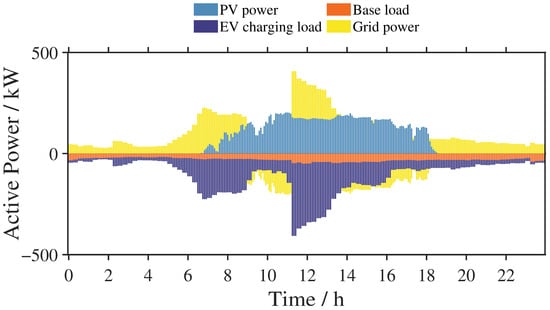
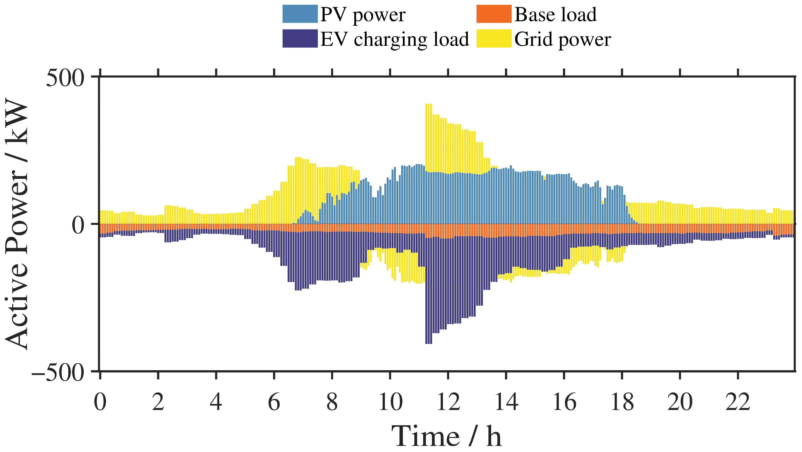
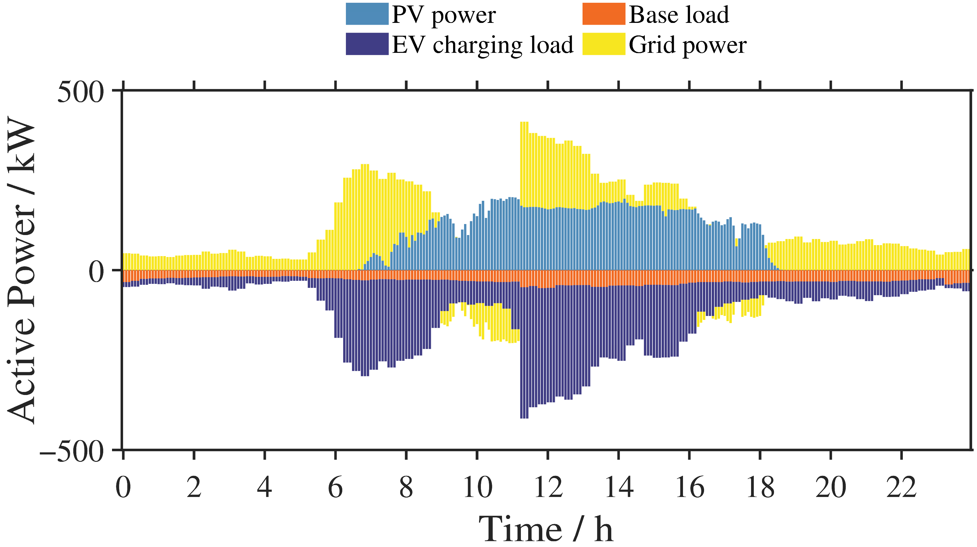
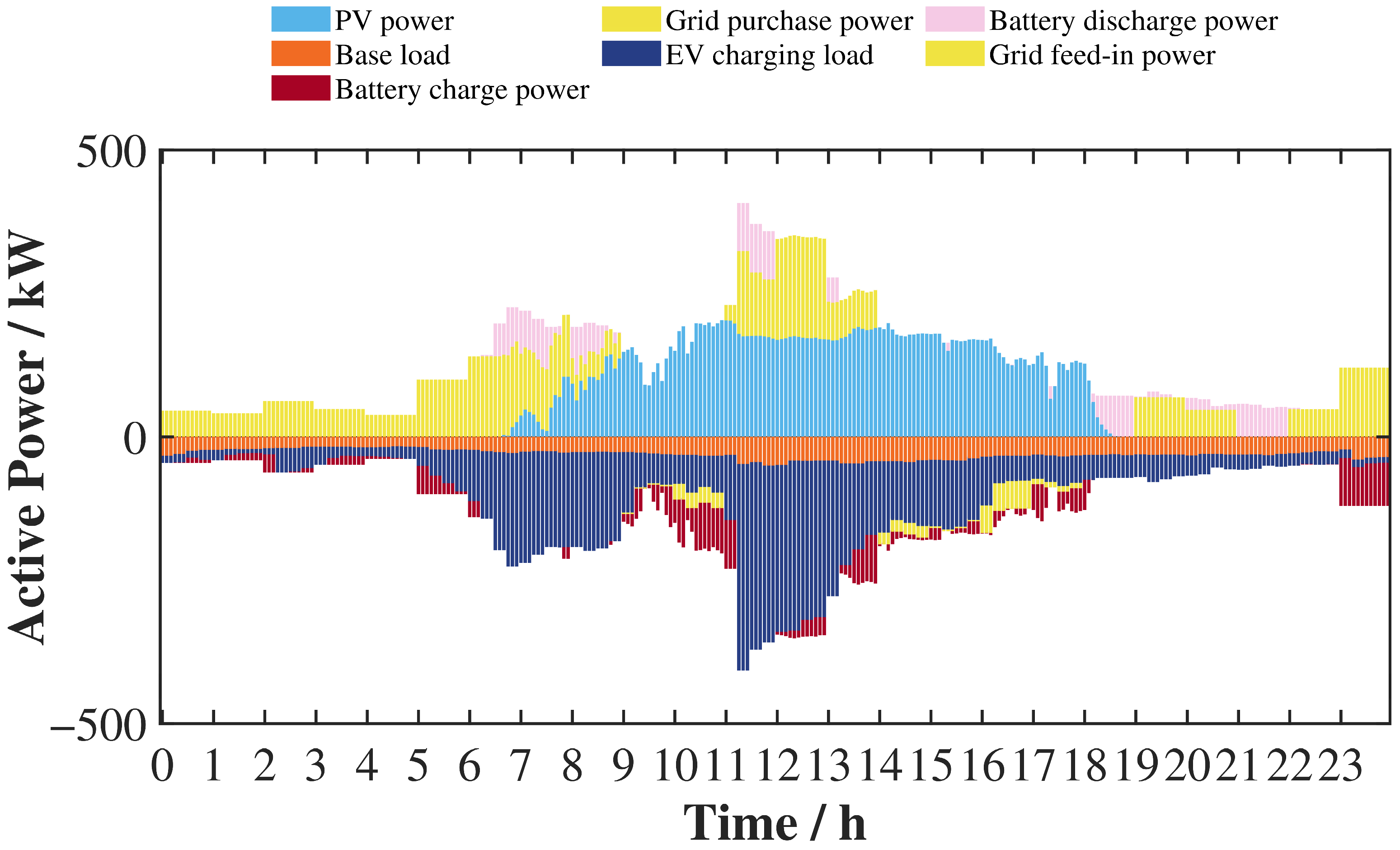
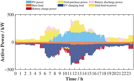
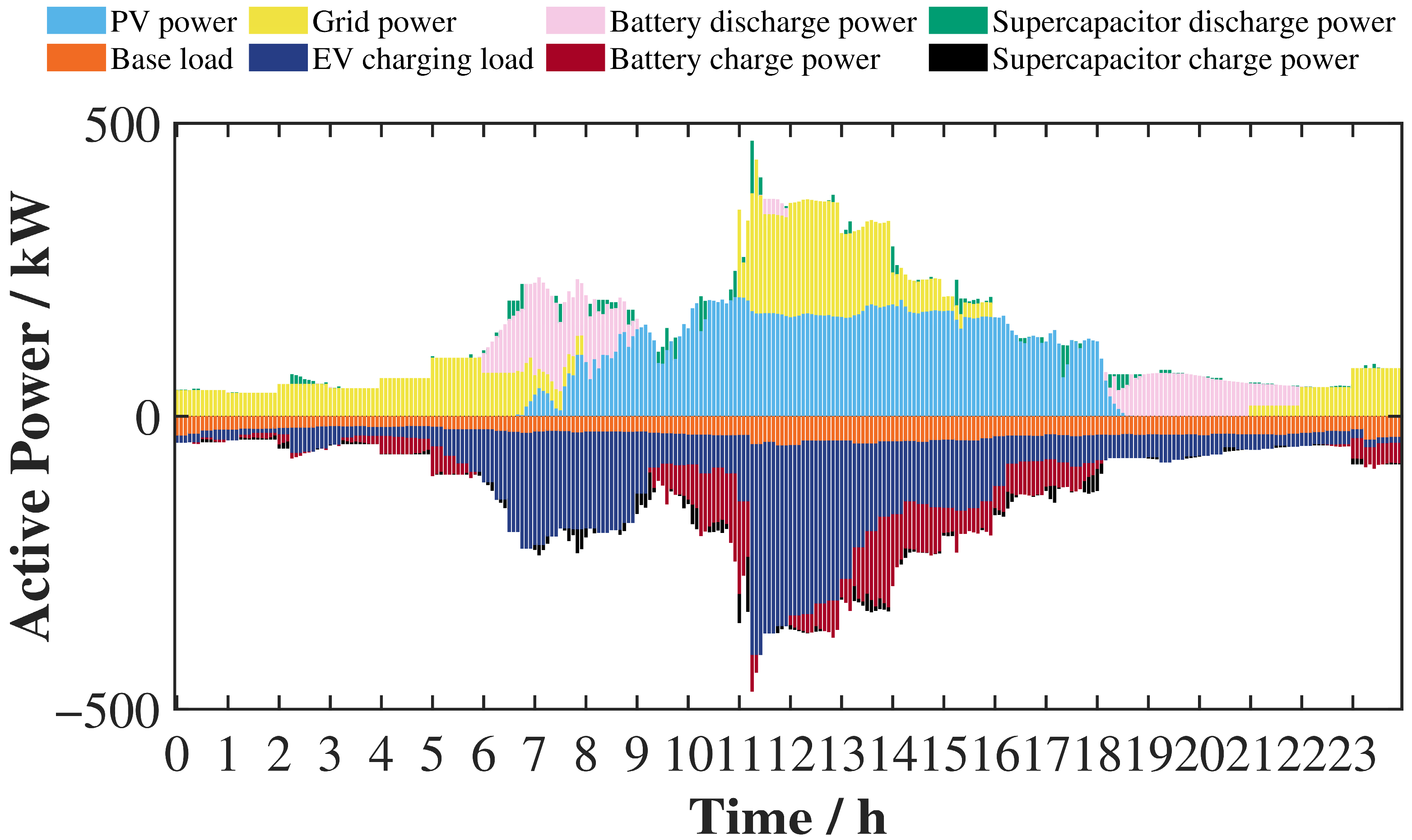
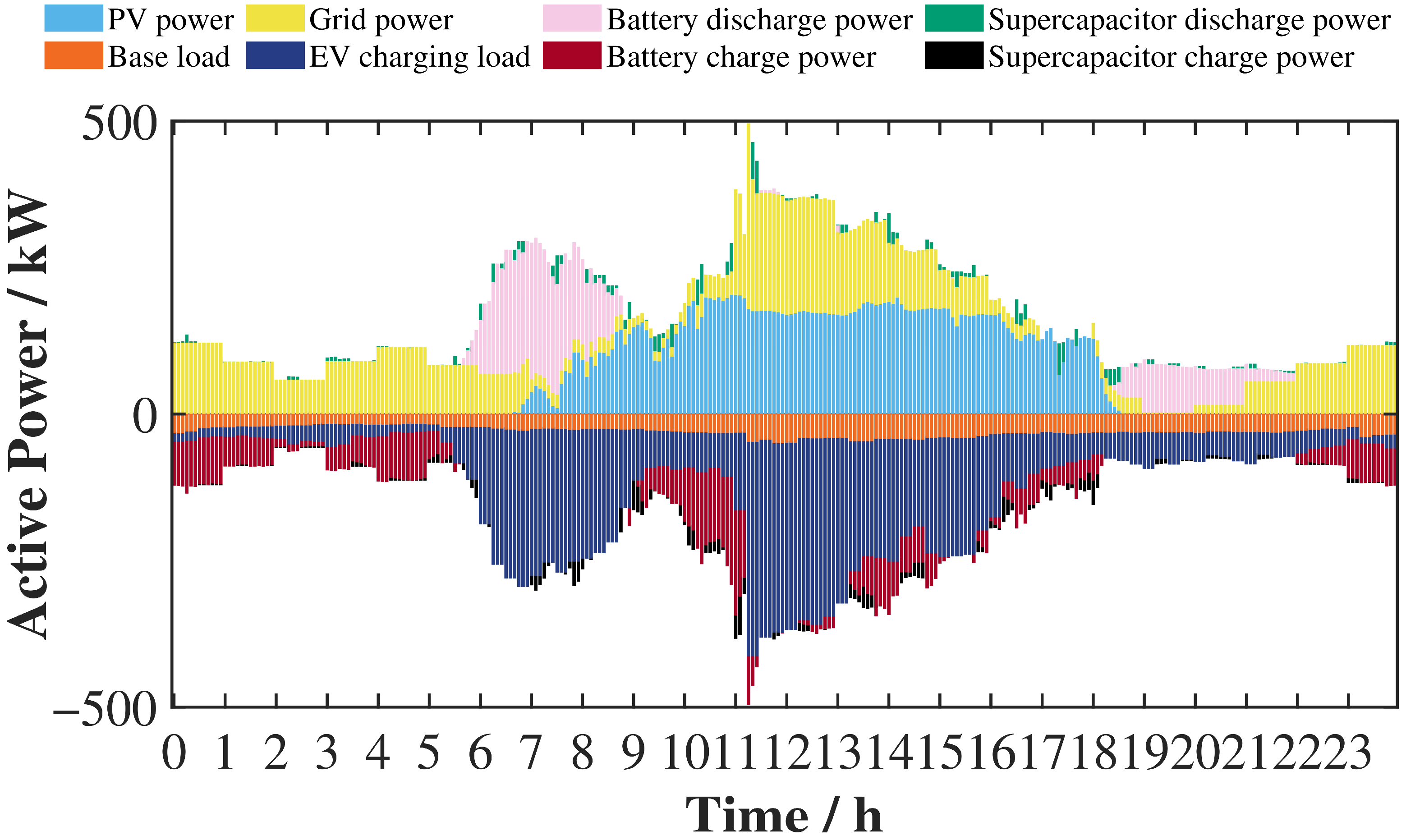
Before energy storage is configured, the power dispatch results for the two typical days in the commercial-area scenario are shown in Figure 7 and Figure 8.
Figure 7.
Power profiles before energy storage configuration in the commercial-area scenario on typical day 1.
Figure 8.
Power profiles before energy storage configuration in the commercial-area scenario on typical day 2.
It can be seen that, without energy storage, system power balance relies entirely on the passive regulation of renewable energy output and grid power. Due to the temporal mismatch between photovoltaic output and EV charging load, the grid power exhibits obvious peak-valley fluctuations, and the grid bears the full peak-regulation pressure. Under the no-storage condition, system operating smoothness and renewable energy consumption capability are both limited. Therefore, it is necessary to introduce an energy storage system for active power regulation.
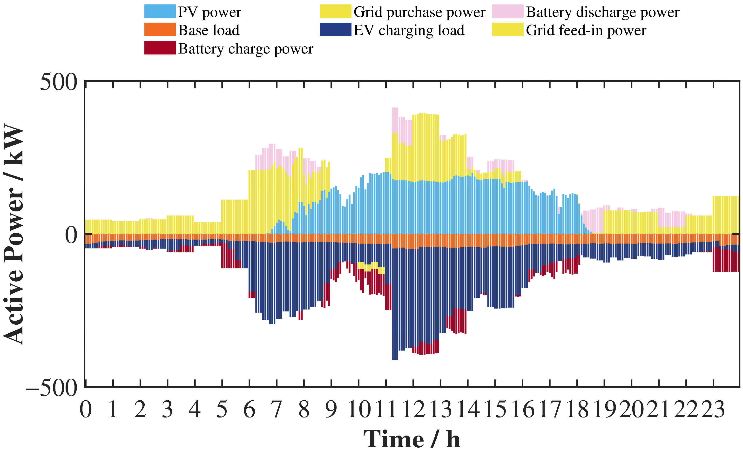
After battery energy storage is configured, the power dispatch results for the two typical days are shown in Figure 9 and Figure 10.
Figure 9.
Power profiles after battery energy storage configuration on typical day 1.
Figure 10.
Power profiles after battery energy storage configuration on typical day 2.
As shown in Figure 9 and Figure 10, under both typical days, the battery energy storage system follows an operating pattern of charging during valley periods and discharging during peak periods. It absorbs energy when photovoltaic output is surplus or the load is low, and releases energy when EV charging demand is concentrated and the system load is high, thereby reducing the peak grid purchase power and improving power allocation. Compared with typical day 1, typical day 2 has stronger load fluctuations, and the battery participates in regulation with a larger amplitude, indicating that energy storage plays a more obvious role in peak shaving and valley filling under high-fluctuation scenarios.
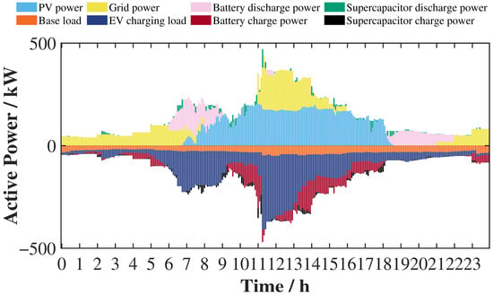
After hybrid energy storage is configured, the power dispatch results for the two typical days are shown in Figure 11 and Figure 12.
Figure 11.
Power profiles after hybrid energy storage configuration on typical day 1.
Figure 12.
Power profiles after hybrid energy storage configuration on typical day 2.
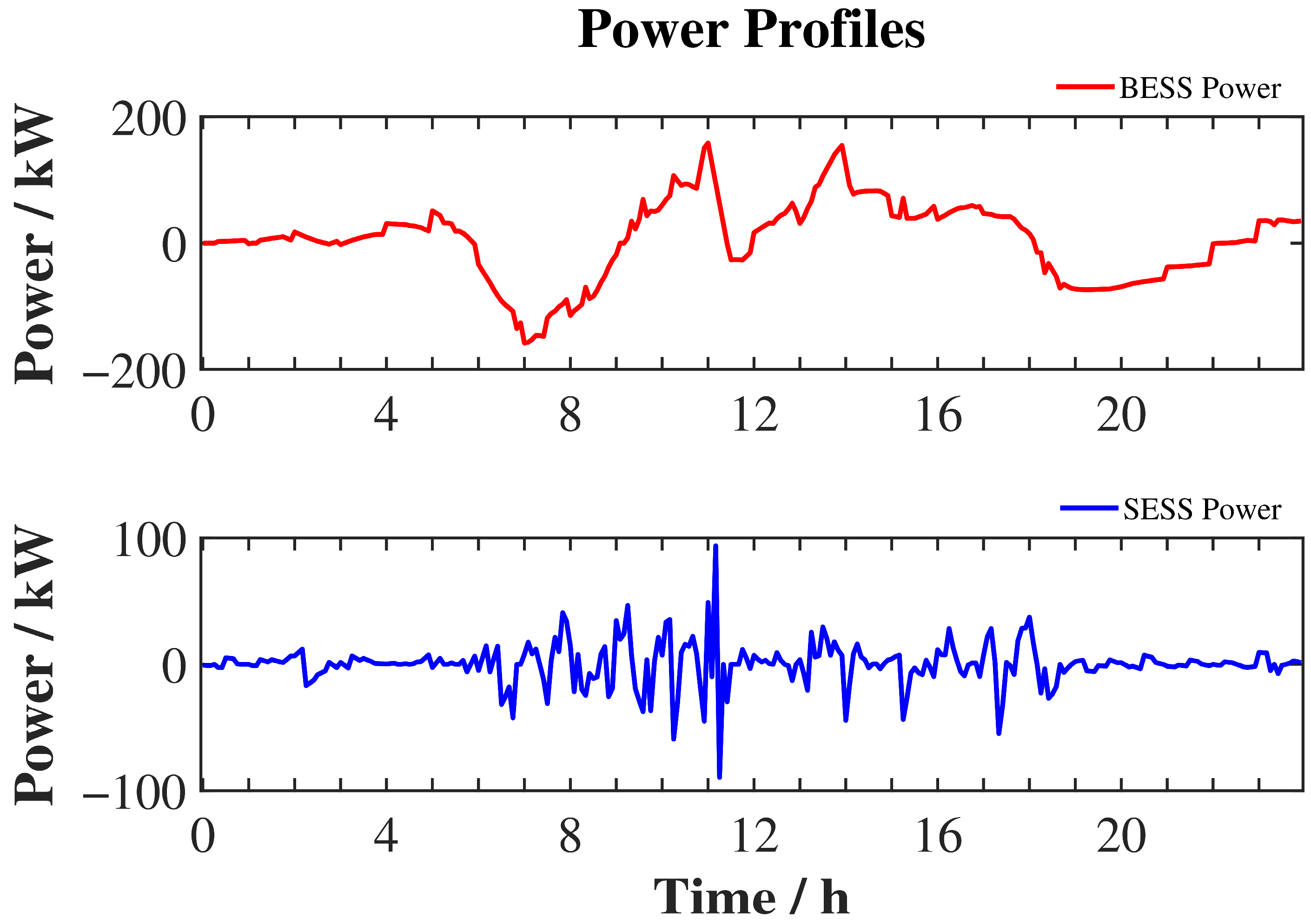
Under both typical days, the hybrid energy storage system exhibits a coordinated characteristic in which the battery mainly regulates energy and the supercapacitor suppresses fluctuations. The system charges during low-load periods or periods with surplus photovoltaic output, and discharges during periods with concentrated EV load and strong fluctuations, thereby improving power allocation and reducing grid-connected power fluctuations. Compared with battery-only energy storage, the supercapacitor in the hybrid energy storage system undertakes more fast-regulation tasks and plays a more significant role in suppressing high-frequency fluctuations, making the overall operation more flexible.
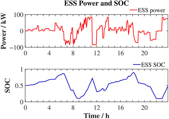
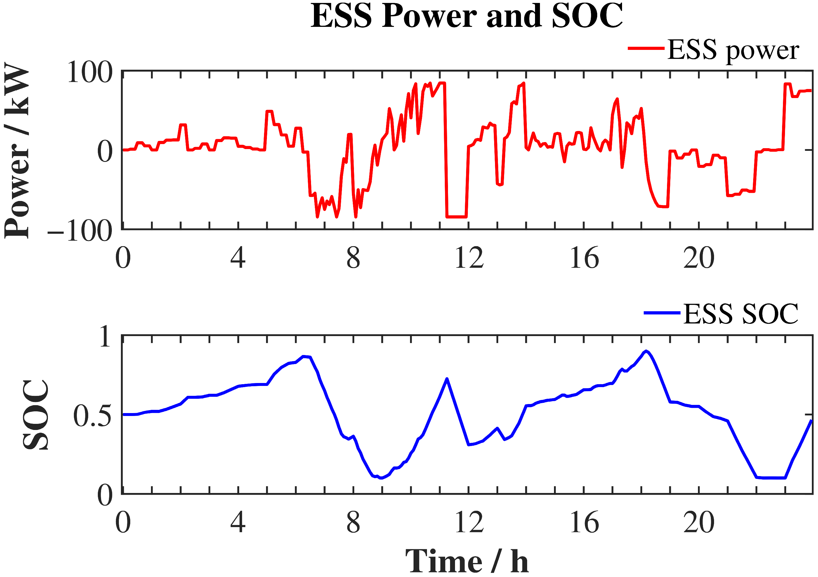
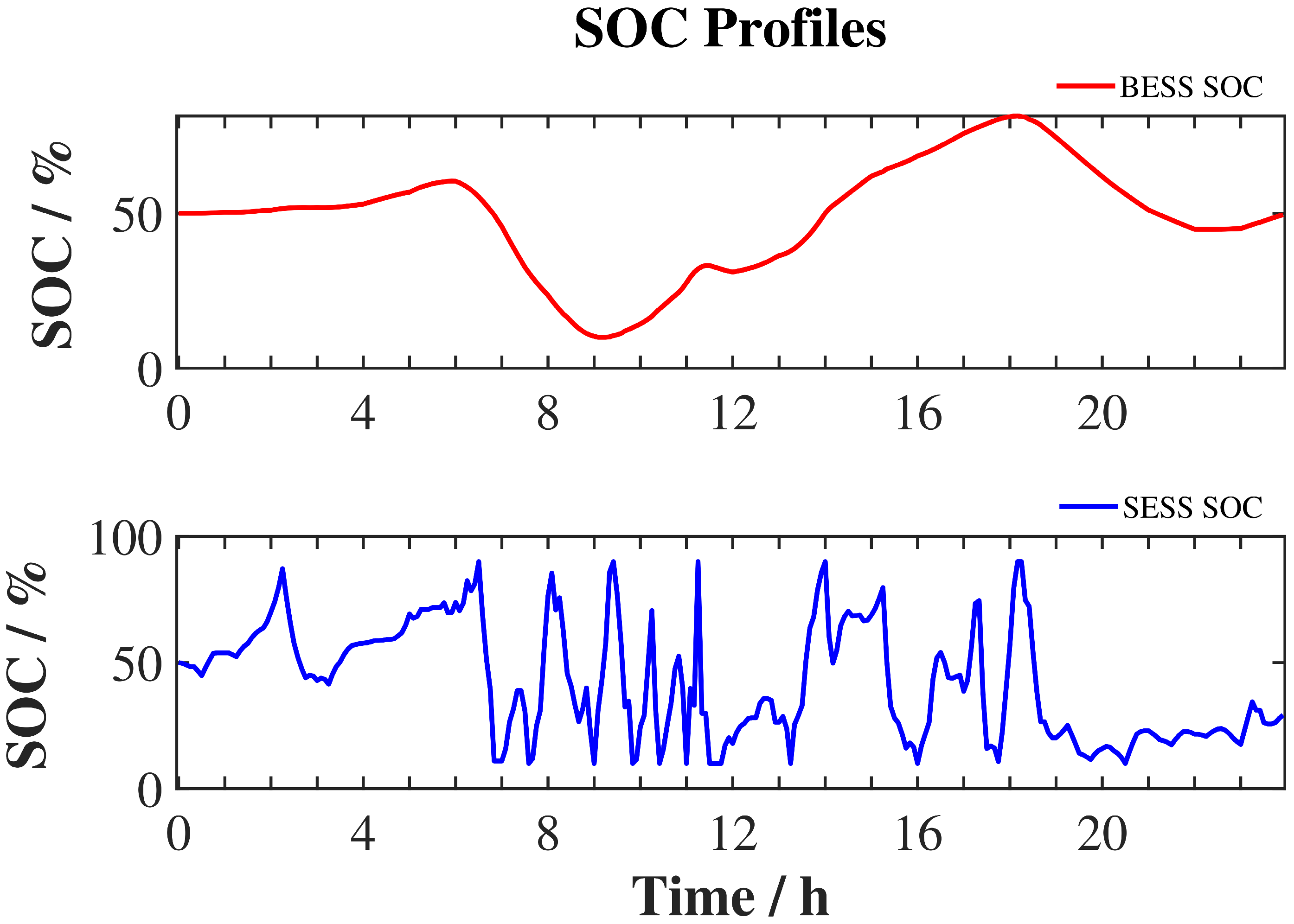
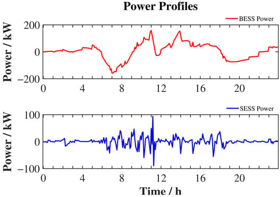
To further analyze the operating characteristics of the energy storage system in each period, the power and SOC curves of the battery-only and hybrid energy storage schemes are further plotted after presenting the overall power allocation results. Typical day 1 is used as an example. By analyzing the charging/discharging power and the evolution of state of charge, the regulation mechanisms of different energy storage schemes can be more intuitively revealed.
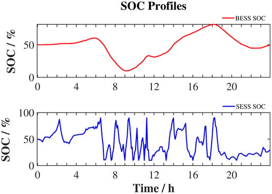
As shown in Figure 13, Figure 14 and Figure 15, when the battery-only energy storage system operates, the battery power fluctuates significantly, and the SOC variation range is relatively wide. This indicates that the battery not only undertakes energy shifting but also participates directly in power fluctuation regulation. By contrast, under the hybrid energy storage configuration, the battery and supercapacitor show a clear coordinated division of tasks. The battery power and SOC vary more smoothly and mainly undertake medium- and low-frequency energy regulation, while the supercapacitor switches power more frequently and responds more rapidly in SOC, mainly suppressing short-term high-frequency fluctuations. Therefore, hybrid energy storage can effectively share the fast-regulation burden of the battery and make the operating characteristics of the energy storage system more reasonable.
Figure 13.
Power and SOC profiles of the battery energy storage system.
Figure 14.
SOC profiles of the battery and supercapacitor in the hybrid energy storage system.
Figure 15.
Power profiles of the battery and supercapacitor in the hybrid energy storage system.
5.4. Algorithm Comparison and Sensitivity Analysis
Additional numerical evaluations are provided in Appendix C
and Appendix D to assess the optimization algorithm and the sensitivity of the coordinated sizing results. Appendix C
and Appendix D present supplementary numerical experiments under a separate parameter setting. Their results are compared within the supplementary case and are not used to calculate the performance improvements reported in Section 5.2. Appendix C presents comparisons with alternative optimization algorithms and statistics from 20 independent runs using random seeds from 1 to 20. The compared algorithms use the same population size, maximum number of iterations, decision-variable bounds, and feasibility-handling procedures. Their performance is evaluated using the best, mean, and standard deviation of the final objective-function values, together with computation time and convergence behavior.
To examine the effects of key parameters, sensitivity analyses of electricity prices, PV output, load magnitude, the penalty factor, and battery degradation parameters are presented in Appendix D. A fixed-lifetime model and different battery ramp constraints are also compared.
6. Discussion
Our study develops a bi-level framework for the coordinated sizing of transformers, batteries, and supercapacitors in a PV-integrated ultra-fast EV charging station. The planning model minimizes the average daily comprehensive cost. The dispatch model considers operating cost, grid-power fluctuations, and storage operating constraints. Rainflow counting and a DOD-dependent cycle-life curve link battery cycling to the annualized battery investment cost.
The case-study results indicate that coordinating storage operation with transformer sizing can reduce transformer capacity requirements and daily cost. Battery-only storage provides effective peak shaving and valley filling. Hybrid storage achieves lower cost, smaller within-hour grid-power deviations, and lower battery cycling damage in the reported comparisons. Its peak–valley reduction is weaker than that of battery-only storage. The preferred configuration therefore depends on the relative importance of economy, power smoothing, and battery degradation.
The battery and supercapacitor provide complementary regulation capabilities under the adopted dispatch strategy. Limiting rapid changes in battery power allows the supercapacitor to take a greater share of short-term regulation. Battery capacity also differs between the two storage schemes. The observed reduction in cycling damage reflects both the capacity selection and the dispatch strategy. A comparison with equal battery capacities is needed to quantify the contribution of the supercapacitor separately.
The supplementary analyses show similar final objective values for PSO, QPSO, and improved QPSO, with a modest early-convergence advantage for improved QPSO in this case. The sensitivity results show that economic performance depends on electricity prices, generation and load levels, the service-penalty setting, and battery degradation assumptions. Lower cost may involve more unserved charging demand. The ramp-constraint comparison also indicates a trade-off between cost and estimated battery lifetime.
Several limitations require further investigation. Battery lifetime is currently estimated from cycling damage alone. Future work should include calendar aging, temperature, and charge–discharge-rate effects. The cycle-life relationship should be validated over the shallow-cycle range encountered in dispatch. A common project horizon with explicit battery replacement costs and residual values would also provide a more complete economic assessment. Cooling-system electricity use and costs should be included when suitable equipment data are available.
The supercapacitor model represents aggregate cell energy and power limits. A practical bank design requires the selection of series–parallel arrangements, operating voltage, converter ratings, and allowable current. Future work should check voltage variation, thermal limits, cell balancing, and conversion losses across the operating range. Installation costs and space requirements should be included in the sizing comparison. These checks are needed to translate the aggregate capacity results into an implementable equipment configuration.
The treatment of charging service also needs further development. Unserved charging demand is currently discarded within each interval and assigned an economic penalty. Future work should examine minimum service requirements and limits on unserved energy. A model with vehicle arrival times, departure times, and required charging energy could distinguish demand that can be delayed from demand that must be curtailed. This would allow the cost savings to be assessed against service quality more directly.
The present case uses two representative days from a limited historical dataset. Their use for annual cost and lifetime estimation assumes that the observed cluster proportions remain representative throughout the year. Additional seasonal data are needed for out-of-sample testing and uncertainty analysis of EV demand and PV generation. Chronological multi-day simulation would also capture energy and power transitions between days. Higher-resolution measurements are needed to assess rapid load changes, since repeating 15 min values at 5 min intervals does not recover fluctuations within the original intervals.
Further evaluation should include equal-capacity storage comparisons, additional station types, and larger sets of independent optimization runs. These tests would help assess the consistency of the sizing results and the computational benefit of improved QPSO. Field measurements or hardware-in-the-loop experiments are also needed to evaluate the dispatch strategy under converter dynamics, measurement errors, and communication delays. The present results support planning comparisons under the stated assumptions; practical performance remains to be verified.
Author Contributions
Investigation and writing—original draft, H.Z.; writing—review and editing, H.W.; resources, L.C.; Supervision, Y.Z.; data curation, Y.L.; conceptualization, Y.S. All authors have read and agreed to the published version of the manuscript.
Funding
This research was funded by State Grid Anhui Electric Power Co., Ltd., Hefei Power Supply Company (contract No. 5212A0250001). The article processing charge (APC) was funded by Hefei University of Technology.
Data Availability Statement
The data and MATLAB (2019) code that support the findings of this study are available from the Corresponding Author, Y.L., upon reasonable request.
Conflicts of Interest
Authors Hao Zhang, Haiwei Wang, Lu Chen, and Yang Zhang were employed by Hefei Power Supply Company, State Grid Anhui Electric Power Co., Ltd. The company provided funding for this research and participated in the study through the contributions of its employed co-authors, as detailed in the Author Contributions section. The remaining authors, Yu Liu and Yong Shi, declare no additional commercial or financial relationships that could be construed as a potential conflict of interest. The authors declare no other conflicts of interest.
Appendix A
According to the standard QPSO formulation [29,30], the local attractor of particle i in dimension j is defined as:
where pi,j(t) is the local attractor, φ is the weighting coefficient, Pi,j(t) is the historical best position of particle i, and Gj(t) is the global best position. The trade-off between the historical best position and the global best position is adjusted by φ:
where c1 and c2 are learning factors, and r1 and r2 are random numbers uniformly distributed in (0, 1). The potential well length determines the search range of a particle. The potential well length L(t) is calculated as:
where Li,j(t) is the potential well length of particle i in dimension j; β is the contraction-expansion coefficient; Cj(t) is the mean best position of all particles; and Xi,j(t) is the current position of particle i.
where M is the number of particles. The mean best position Cj(t) reflects the overall search trend of the particle swarm.
pi,j(t) = φi,j(t) ⋅ Pi,j(t) + [1 − φi,j(t)] ⋅ Gj(t),
Li,j(t) = 2β|Cj(t) − Xi,j(t)|,
A particle moves in a one-dimensional δ potential well centered at point p, and its position is determined by the following equation:
where X is the new position of the particle, p is the local attractor of the particle, L is the potential well length, and u is a random number uniformly distributed in [0, 1].
X = p ± 0.5 ⋅ L ⋅ ln(1/u),
By extending Equation (A3) to dimension j in combination with Equation (A5), the particle position update equation is obtained as:
where Xi,j(t + 1) is the updated position of particle i in dimension j. According to Equation (A6), each particle performs a stochastic search around the local attractor, while the search range is scaled by the distance between the current particle position and the mean best position.
Xi,j(t + 1) = pi,j(t) ± β[Cj(t) − Xi,j(t)]ln(1/u),
Although standard QPSO has a relatively simple structure and good global search capability, its performance may be affected by uneven initial population distribution and the fixed contraction-expansion coefficient. Therefore, two lightweight improvements are introduced in this study, including Sobol-sequence population initialization and a nonlinear contraction-expansion coefficient.
where si,j ∈ [0, 1] is generated using the Sobol low-discrepancy sequence. Compared with pseudo-random initialization, the Sobol sequence provides a more uniform distribution of particles in the feasible search space and improves the coverage of candidate sizing solutions.
where t is the current iteration number, and Tmax is the maximum number of iterations. A relatively large value of β(t) is maintained during the early search stage to enhance global exploration, while β(t) gradually decreases as the iteration proceeds to strengthen local exploitation and convergence accuracy.
Xi,j(t + 1) = pi,j(t) ± β(t)[Cj(t) − Xi,j(t)]ln(1/u).
With the above two modifications, the improved QPSO retains the basic search mechanism of standard QPSO while enhancing initial population coverage and the balance between exploration and exploitation. The improved algorithm is used only as the numerical optimizer for the upper-level sizing problem.
Table A1.
Parameter settings of the improved QPSO algorithm.
The local-attractor weighting coefficients are set to c1 = c2 = 2, giving equal nominal importance to the personal-best and global-best positions. Each run terminates after Tmax = 50 iterations, without an additional early-stopping criterion. Before each fitness evaluation, the battery and supercapacitor unit counts are rounded to the nearest integers, while the transformer rating remains a continuous variable. Candidate solutions are repaired by clipping each decision variable to its prescribed lower and upper bounds. If the lower-level scheduling problem is infeasible, the candidate solution is assigned an infinite fitness value and is not used to update the personal-best or global-best positions.
To assess the variability of the stochastic optimization results, 20 independent runs are performed using random seeds from 1 to 20. At the beginning of each run, the MATLAB random number generator is initialized using ‘rng(seed,’twister’)’. The same population size, maximum number of iterations, variable bounds, and feasibility-handling procedures are used for all compared algorithms.
Appendix B
This appendix presents the auxiliary variables and linear constraints used in the lower-level dispatch model. For each lower-level solve, the transformer rating and storage-unit numbers are fixed at the values supplied by the upper-level model. The formulation applies separately to each representative day; the representative-day index is omitted for clarity. Dispatch intervals are indexed by j = 1,…,T, and hours by h = 1,…,24.
Appendix B.1
The mean grid-connected power within hour h is:
where Ωh denotes the set of dispatch intervals within hour h, and Nh is its cardinality. For the 5 min dispatch interval used in this study, Nh = 12. A nonnegative auxiliary variable zj is introduced with the following linear constraints:
zj ≥ 0,
The hourly average deviation and full-day fluctuation index are represented in the optimization model as:
The hourly deviation constraint is:
Dgrid,h ≤ 0.1PTRS + Ptol,
The same auxiliary variables are used in the objective and the hourly deviation limit. Since the fluctuation term has a positive coefficient in the minimization objective, these variables can attain the corresponding absolute deviations at optimality. Constraints (A11)–(A13) alone impose lower bounds; equality with the absolute deviations follows from their minimization. Thus, the reformulation preserves the original absolute-deviation objective and constraint without requiring additional binary variables.
Appendix B.2
The transformer apparent-power rating STR is expressed in kVA. Under the adopted constant power-factor assumption, its allowable active-power magnitude is PTRS = k∙STR, in kW. The apparent-power constraint can therefore be expressed using two linear inequalities:
Positive grid power denotes import and negative grid power denotes export. If export is prohibited, the additional constraint ≥ 0 is imposed.
Appendix B.3
Binary indicators and represent the battery charging and discharging states. Their power limits and exclusivity constraints are:
The corresponding supercapacitor constraints are:
Here, NESS and NSC are the configured battery and supercapacitor unit numbers, respectively, and PSC,R is the rated power of one supercapacitor unit. These constraints allow charging, discharging, or idle operation while preventing simultaneous charging and discharging within either device. Because storage-unit numbers are fixed during each lower-level solve, their products with binary indicators are linear expressions.
After the above reformulations, the lower-level objective and operational constraints are linear in the dispatch variables, with binary variables describing the storage operating states. The normalization denominators in Section 3.2.1 are fixed, positive reference values. The moving-average decomposition is calculated from the prescribed net-load profile before dispatch optimization and supplies fixed reference profiles. Battery rainflow counting and lifetime estimation are performed using the resulting SOC trajectories for upper-level economic evaluation; they are not embedded as nonlinear expressions in the lower-level optimization. Accordingly, for each fixed upper-level configuration, the lower-level dispatch problem is a mixed-integer linear program.
Appendix C
The improved QPSO algorithm is compared with standard QPSO and PSO using the same population size, iteration limit, and constraint-handling procedures to evaluate optimization performance and robustness. Each algorithm is run independently 20 times. The best objective value at each iteration is recorded for each run. These values are averaged across the 20 runs to obtain the convergence curves in Figure A1.
Figure A1.
Algorithm comparison.
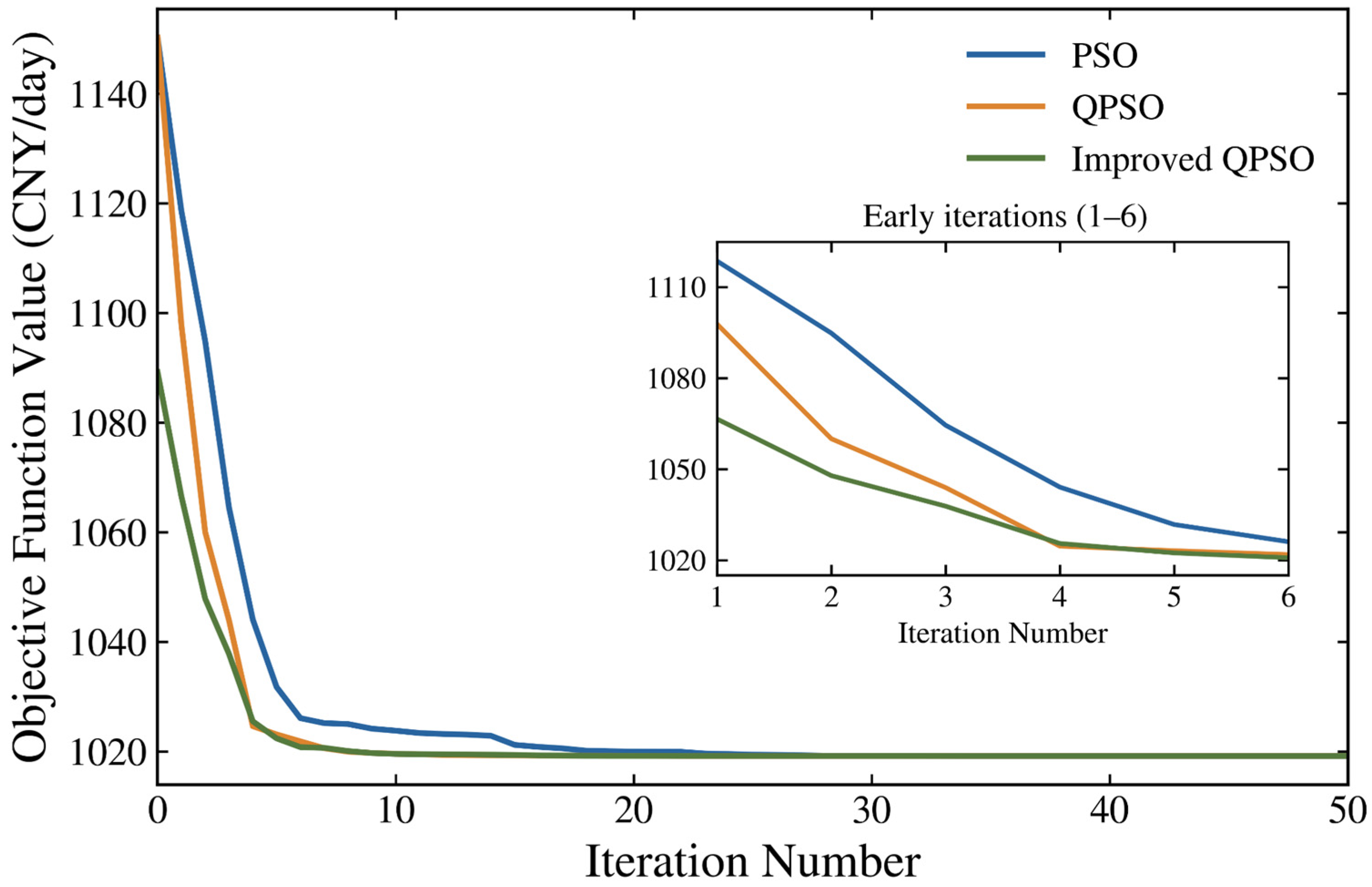
To be honest, the three algorithms achieve nearly identical final objective values in this case. But the improved QPSO shows a modest advantage in the early iterations, suggesting that the modified initialization and search strategy may help identify promising solutions sooner. So its benefit is mainly in the early search stage, with no substantial improvement in the final solution observed.
Appendix D
A one-at-a-time sensitivity analysis is conducted for electricity prices, PV output, load magnitude, unmet-demand penalty factor, and battery cycle life. Each factor is varied to 80%, 100%, and 120% of its baseline, while other inputs remain unchanged. These levels are illustrative rather than statistical confidence limits. Purchase and export prices, as well as base and EV loads, are scaled together. Battery cycle life is adjusted by scaling the fitted (N(DOD)) curve. Each scenario is re-optimized using improved QPSO with 30 particles, 50 iterations, and three fixed random seeds, reporting the best result.
Figure A2 shows the changes in cost, battery sizing, estimated lifetime, and unserved charging energy. Reducing electricity prices by 20% lowers the daily comprehensive cost by 11.97%, while increasing them by 20% raises it by 11.11%. Battery capacity and lifetime also change as each scenario is re-optimized. These results reflect both the parameter variations and the resulting dispatch and sizing decisions.
Figure A2.
Sensitivity analysis: (a) daily comprehensive cost; (b) battery capacity; (c) estimated battery lifetime; (d) unserved EV charging energy.
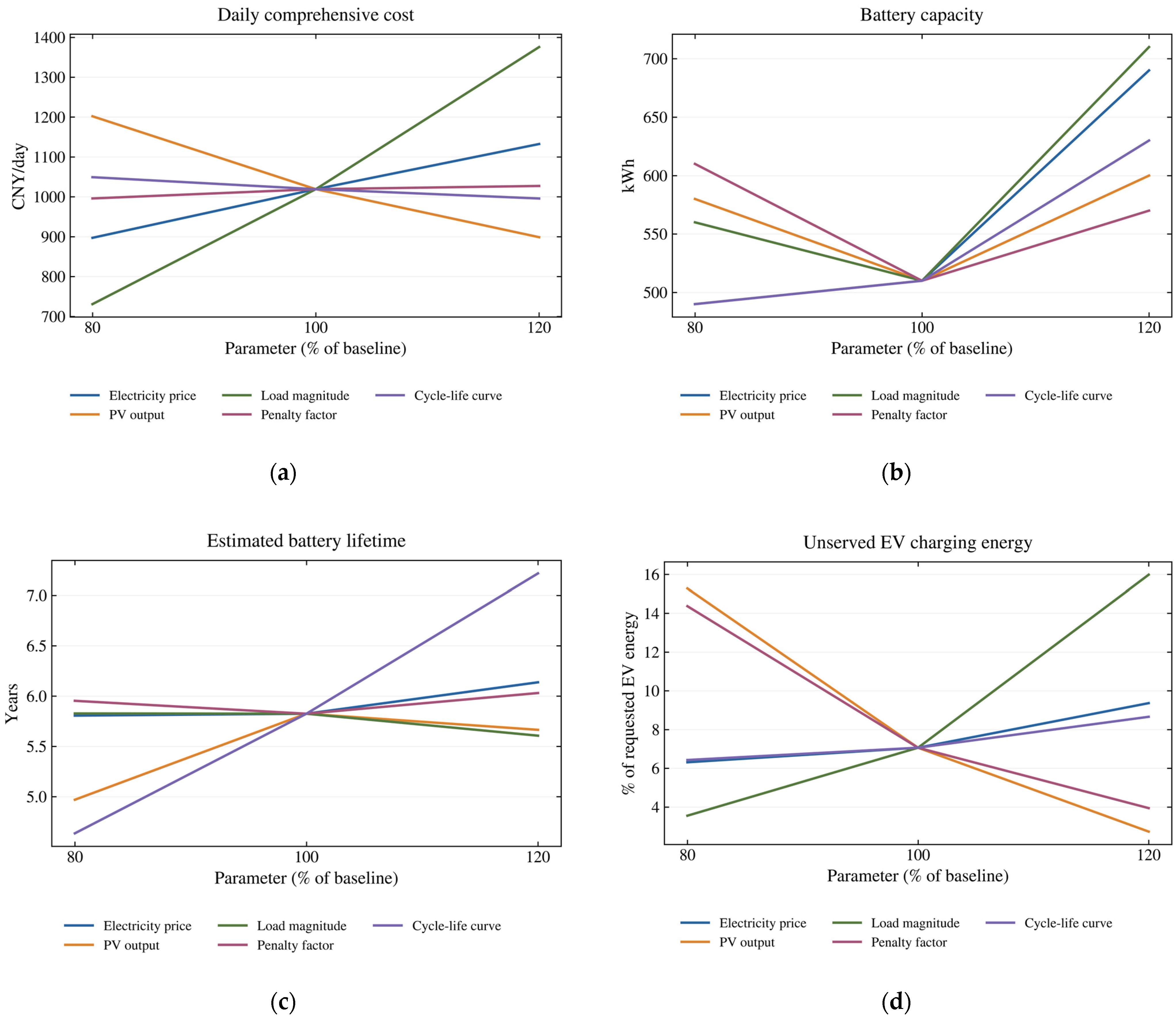
The baseline unserved EV-energy fraction is 7.06%. It rises to 14.37% when the penalty factor is reduced by 20% and falls to 3.94% when the factor is increased by 20%. A lower cost can therefore come with less charging demand being served. Cost and charging-service fulfillment should be assessed together.
A fixed-lifetime model is used to examine the effect of degradation-dependent battery cost. The battery lifetime is fixed at the baseline estimate of 5.8242 years during sizing, and battery investment cost is retained. Both designs are then reassessed using the original degradation-aware model.
Table A2.
Comparison of degradation-aware and fixed-lifetime sizing.
After reassessment, the fixed-lifetime design has a 0.75% higher daily cost. The difference is modest for this case, where the fixed lifetime is set to the degradation-aware baseline estimate.
The battery ramp limit is set to 0.05, 0.10, and 0.20 of rated power per 5 min interval. A case without the ramp constraint is also tested. Each case is re-optimized with all other operating constraints unchanged. The ramp limit applies within each representative day; inter-day power transitions are excluded.
Figure A3.
Effects of the within-day battery ramp constraint on system sizing and operating performance.
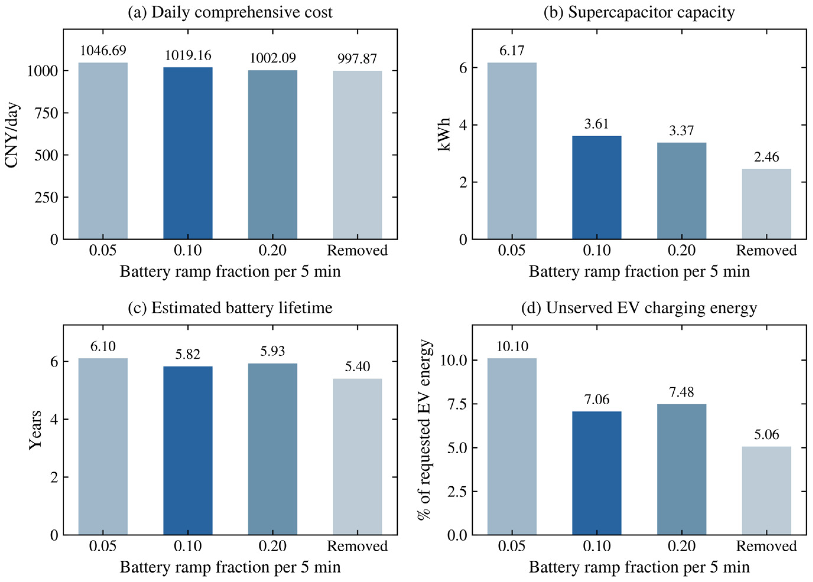
Table A3.
Optimized capacities under different battery ramp constraints.
Removing the ramp constraint reduces daily cost by 2.09% and estimated battery lifetime by 7.30% relative to the baseline. Tightening the ramp fraction to 0.05 increases cost by 2.70% and lifetime by 4.73%. These changes include the effects of re-optimizing storage capacities.
The representative-day-weighted mean of the 24 hourly mean absolute deviations is below 10−8 kW in all four cases. Grid power is nearly constant within each hour under the adopted dispatch objective, but it can still change between hours.
References
- Xinhua News Agency; CPC Central Committee; State Council. Opinions on Fully, Accurately and Comprehensively Implementing the New Development Philosophy and Promoting Carbon Peaking and Carbon Neutrality. 2021. Available online: https://www.gov.cn/zhengce/2021-10/24/content_5644613.htm (accessed on 25 August 2026).
- Ruan, Q.; Mei, S.; Huang, X.; Chen, Y. Challenges and Research Prospects of Resilience Enhancement of Low-carbon Power Grid. Proc. CSEE 2022, 42, 2819–2830. [Google Scholar] [CrossRef]
- Chen, Y.; Tian, H.; Liu, Y.; Chen, Y.; Li, C.; Si, Y.; Bao, Y. Robust Optimization Configuration of Photovoltaic-storage-charging Integrated System in Expressway Service Area Considering Demand Response of Electric Vehicles. Proc. CSEE 2025, 45, 1752–1767. [Google Scholar] [CrossRef]
- Shao, Y.; Mu, Y.; Yu, X.; Dong, X.; Jia, H.; Wu, J.; Zeng, Y. A Spatial-temporal Charging Load Forecast and Impact Analysis Method for Distribution Network Using EVs-Traffic-Distribution Model. Proc. CSEE 2017, 37, 5207–5219, 5519. [Google Scholar] [CrossRef]
- Cao, W. Research on Electric Vehicle Charging Load Forecasting Methods and Applications. Master’s Thesis, Nanjing University of Posts and Telecommunications, Nanjing, China, 2020. [Google Scholar] [CrossRef]
- Wang, R.; Gao, X.; Li, J.; Xu, J.; Ai, G.; Jing, X. Electric vehicle charging demand forecasting method based on clustering analysis. Power Syst. Prot. Control 2020, 48, 37–44. [Google Scholar] [CrossRef]
- Guo, C.; Zhu, K.; Chen, C.; Xiao, X. Characteristics and effect laws of the large-scale electric vehicle charging load. ETransportation 2020, 3, 100049. [Google Scholar] [CrossRef] [Scilit]
- Ding, M.; Xie, J.; Liu, X.; Shi, W. The Generation Method and Application of Wind Resources/Load Typical Scenario Set for Evaluation of Wind Power Grid Integration. Proc. CSEE 2016, 36, 4064–4072. [Google Scholar] [CrossRef]
- Mets, K.; Depuydt, F.; Develder, C. Two-stage load pattern clustering using fast wavelet transformation. IEEE Trans. Smart Grid 2015, 7, 2250–2259. [Google Scholar] [CrossRef] [Scilit]
- Zhang, Y.; Yang, L.; Ge, S.; Chen, J. Short-term photovoltaic power forecasting based on Kmeans algorithm and support vector machine. Power Syst. Prot. Control 2018, 46, 118–124. [Google Scholar]
- Ding, Q.; Zhao, B.; Chen, Z.; Zhang, X.; Guo, L.; Xiang, J. Coordinated Configuration Optimization of Hybrid Electric-hydrogen Energy Storage in Microgrids Based on Multi-time Scale Feature Extraction. Proc. CSEE 2025, 45, 8867–8879. [Google Scholar] [CrossRef]
- Yang, T.; Huang, Y.; He, Z.; Li, Z.; Wang, T. Optimal Configuration of Siting and Sizing for Grid-forming Battery Energy Storage Station Based on Multi-timescale Regulation. Autom. Electr. Power Syst. 2024, 48, 54–64. [Google Scholar]
- Zhao, Y.; Wang, H.; He, B.; Xu, W. Optimization Strategy of Configuration and Operation for User-side Battery Energy Storage. Autom. Electr. Power Syst. 2020, 44, 121–128. [Google Scholar]
- Narimani, M.R.; Asghari, B.; Sharma, R. Energy storage control methods for demand charge reduction and PV utilization improvement. In Proceedings of the 2017 IEEE PES Asia-Pacific Power and Energy Engineering Conference (APPEEC), Bangalore, India, 8–10 November 2017; pp. 1–5. [Google Scholar]
- Lu, H. Research on Optimal Configuration and Comprehensive Value Evaluation of Energy Storage in New Power Systems. Master’s Thesis, North China Electric Power University, Beijing, China, 2021. [Google Scholar] [CrossRef]
- Liu, J.; Qin, B.; Cai, Q.; Ding, T.; Li, H. Capacity Planning of Energy Storage for Urban Rail Transit Systems Considering Renewable Energy Integration. Power Syst. Technol. 2025, 49, 709–718. [Google Scholar] [CrossRef]
- Zou, Y.; Shi, S.; Yao, Y.; Huang, Y.; Fang, M.; Jin, T. Optimal allocation of energy storage bi-level based on improved scenario generation method for ac-dc hybrid distribution network. Acta Energ. Sol. Sin. 2025, 46, 521–531. [Google Scholar] [CrossRef]
- Lu, Y.; He, Z.; Li, Y.; Cui, L.; Xu, T. Bi-level optimization for capacity allocation of integrated energy systems considering wind-solar uncertainty. Power Syst. Prot. Control 2025, 53, 127–138. [Google Scholar] [CrossRef]
- Li, B.; Wang, X.; Guo, Q. Bi-layer Optimal Configuration Method for Mobile Energy Storage Interconnection Devices in Joint Scenario of Distribution Network. Autom. Electr. Power Syst. 2025, 49, 143–153. [Google Scholar]
- Zhang, Y.; Hao, S. Optimal configuration of transformer capacity and energy storage for electric vehicle charging stations. Electr. Meas. Instrum. 2023, 60, 19–25. [Google Scholar] [CrossRef]
- Chen, B.; Lü, Y.; Chen, K.; Sha, Z.; Liu, X.; Liu, Y. Research Progress of Solid-state Supercapacitors Electrolytes and Its Classifications. High Volt. Eng. 2019, 45, 929–939. [Google Scholar] [CrossRef]
- Chen, B.; Zhao, J. Research progress on influencing factors and mechanisms of cycle life of lithium ion batteries. Chin. J. Power Sources 2025, 49, 57–66. [Google Scholar]
- Li, X.; Ma, R.; Wang, S.; Zhang, Y.; Li, B.; Fang, C. Operation Control Strategy for Energy Storage Station After Considering Battery Life in Commercial Park. High Volt. Eng. 2020, 46, 62–70. [Google Scholar]
- Downing, S.D.; Socie, D.F. Simple rainflow counting algorithms. Int. J. Fatigue 1982, 4, 31–40. [Google Scholar] [CrossRef] [Scilit]
- National Development and Reform Commission; National Energy Administration. Deepening the Market-Oriented Reform of Feed-in Tariffs for New Energy; National Development and Reform Commission: Beijing, China; National Energy Administration: Beijing, China, 2025. Available online: https://www.ndrc.gov.cn/xxgk/jd/jd/202502/t20250209_1396070.html (accessed on 25 August 2026).
- GB/T 19964-2024; Technical Requirements for Connecting Photovoltaic Power Stations to Power Systems. Standards Press of China: Beijing, China, 2024.
- Tian, B.; Zhang, Z.; Yang, M. Research on Hybrid Energy Storage Power Allocation and Capacity Determination Based on Multiple Moving Average Filtering. Trans. China Electrotech. Soc. 2024, 39, 1548–1564. [Google Scholar] [CrossRef]
- Chen, J. Research on Identification Method for Distribution Transformer Winding Material Based on K-Means Clustering. Master’s Thesis, North China Electric Power University, Beijing, China, 2024. [Google Scholar] [CrossRef]
- Clerc, M.; Kennedy, J. The particle swarm: Explosion, stability, and convergence in a multidimensional complex space. IEEE Trans. Evol. Comput. 2002, 6, 58–73. [Google Scholar] [CrossRef] [Scilit]
- Sun, J. Research on Quantum-Behaved Particle Swarm Optimization Algorithm. Ph.D. Thesis, Jiangnan University, Wuxi, China, 2009. [Google Scholar]

Disclaimer/Publisher’s Note: The statements, opinions and data contained in all publications are solely those of the individual author(s) and contributor(s) and not of MDPI and/or the editor(s). MDPI and/or the editor(s) disclaim responsibility for any injury to people or property resulting from any ideas, methods, instructions or products referred to in the content. |
© 2026 by the authors. Licensee MDPI, Basel, Switzerland. This article is an open access article distributed under the terms and conditions of the Creative Commons Attribution (CC BY) license.