Research on Incremental Global Optimization Model Predictive Current Control for Dual Three-Phase Open-Winding Permanent-Magnet Motors

Abstract

Dual three-phase open-winding permanent-magnet synchronous motor (PMSM) drives offer high DC-bus utilization and fault tolerance, but conventional model predictive current control (MPCC) for this topology suffers from heavy rolling optimization, large harmonic currents, and sensitivity to machine parameters. This paper proposes an incremental global optimization model predictive current control (IGOMPCC) method. First, an incremental prediction equation over adjacent control periods cancels the permanent-magnet flux term in the reference voltage solution, eliminating dependence on the flux-linkage parameter. Second, inverter 1 selects its optimal vector from the 12 outermost large voltage vectors, while inverter 2 locks the reference voltage sector by deadbeat incremental voltage prediction, restricting candidate vector groups to two, with duty cycles solved in closed form by the Lagrange multiplier method; single-cycle cost function evaluations drop from 144 to 3. Third, two adjacent active vectors and a zero vector are synthesized at the analytical duty cycle to fix the equivalent switching frequency, concentrating harmonics and suppressing z₁-z₂ sub-plane currents. Simulation results show that, versus traditional MPCC, the settling time is shortened by 34.1% for a speed step and 20% for a load step, the peak d-axis current fluctuation is reduced by 52.9%, and the q-axis current steady-state error is nearly eliminated.

1. Introduction

With the rapid advancement of new energy technologies dominated by electric energy, increasing attention is being paid to efficient drive technologies for multiphase motors [1,2]. Among these technologies, the open-winding polyphase motor drive system offers significantly improved DC voltage utilization, a higher degree of control freedom, low torque ripple, and strong fault tolerance [3,4]. Because an open-winding system requires simultaneous control of two inverters, its control algorithm is more complex. Multiphase motors have numerous harmonic sub-planes, and the stator current contains a high proportion of harmonics. These harmonics do not contribute effectively to the synthesis of fundamental torque; instead, they induce eddy-current and hysteresis losses in the rotor, reducing motor efficiency and increasing temperature rise. In an asymmetric dual three-phase motor, the two sets of three-phase windings are spatially staggered by an electrical angle of 30°, ensuring that the main low-order current harmonics generated by inverter PWM modulation and current control, such as the fifth and seventh harmonics, have equal amplitudes but opposite phases in the phase currents. Through the superposition of magnetomotive forces, these harmonics cancel each other, significantly suppressing stator harmonic currents and the resulting motor losses and torque ripple and leading to smoother torque output [5,6,7]. This is an advantage of dual three-phase motors.

Reference [8] proposes a finite-control-set model predictive control strategy based on deadbeat control. By subdividing sectors, simplifying the control set, and reducing the number of voltage-vector calculations, this strategy improves the real-time performance and effectiveness of control. Reference [9] introduces a multilevel predictive current control strategy based on virtual vectors, which includes a fundamental control level and a secondary control level responsible for tracking reference currents in two subspaces, respectively. In Reference [10], a special vector is used to modulate the space vector of the dual three-phase motor to improve the XY-plane current at high speed and reduce the steady-state error and total harmonic distortion. However, the aforementioned model predictive current control strategies oversimplify sector division and voltage-vector selection, leading to excessive overshoot during no-load startup of dual three-phase motors. Zero-sequence current in the common-bus topology is also a key control issue. Moreover, the effects of the proposed methods on suppressing zero-sequence current and common-mode voltage are not analyzed in these studies. Reference [11] proposes an improved model predictive torque control strategy. This method synthesizes 18 nonzero virtual voltage vectors and adopts a flux deadbeat prediction strategy to directly calculate the reference voltage vector, reducing the complexity of parameter calculation and enhancing control robustness. Reference [12] introduces a direct torque control scheme that combines the voltage vectors of two inverters to generate three voltage levels, reducing harmonic voltage in the auxiliary plane. Reference [13] adds space-vector pulse-width modulation to deadbeat model predictive torque control, which can effectively suppress harmonic currents while improving torque tracking performance. Torque control requires selecting appropriate voltage vectors in each sector and calculating their projections on the harmonic sub-planes. This process involves many geometric and algebraic operations and, compared with traditional model predictive current control, has higher computational complexity, making real-time control difficult for open-winding dual three-phase motors. Reference [14] proposes an improved model predictive torque control method based on deadbeat control and discrete space-vector modulation, but this method is highly dependent on system parameters. Therefore, Reference [15] proposes a virtual impedance technique to reduce the system’s sensitivity to parameter variations. Reference [16] proposes a global optimization multi-vector control method under deadbeat voltage prediction. It calculates the voltage reference vector by combining the deadbeat prediction method and incorporates the duty-cycle allocation results into the cost function. However, the above control methods have been studied only for conventional dual three-phase motors, and those studies do not address the control performance of these methods in open-winding dual three-phase motors.

In this paper, a new IGOMPCC method is proposed to drive and control the inverters of the drive system. One of the six-phase inverters adopts a deadbeat model predictive current control method in the fundamental sub-plane to directly calculate the optimal voltage vector without rolling optimization using a cost function, thus avoiding the substantial computational burden associated with traditional model predictive methods. The other six-phase inverter determines the sector of the reference voltage vector through deadbeat control, calculates the optimal duty cycle using the Lagrange multiplier method, and finally selects the optimal duty-cycle combination scheme under the constraint of minimizing the cost function. The proposed model predictive control, which combines deadbeat control and the incremental global optimization method, reduces the number of rolling optimizations of the cost function. Inverter 2 uses deadbeat voltage prediction to reduce the alternative voltage-vector set to two groups, avoiding rolling calculation of the duty cycle. The incremental prediction equation removes the dependence on flux linkage, enhancing system robustness and reducing vibration and noise.

It should be noted that Reference [17] is an improved deadbeat MPCC method proposed by our team in an earlier study. The contributions of this paper are reflected in the following three aspects. First, in terms of the prediction model, by constructing the incremental prediction equation of adjacent control periods, the permanent-magnet flux term is canceled through the difference in the reference voltage solution process, and the control process no longer depends on the flux parameter λ_f, which fundamentally overcomes the inherent sensitivity of Reference [17] to motor parameters such as flux. Second, in terms of vector selection and duty-cycle solution, inverter 2 directly locks the reference vector sector by deadbeat incremental voltage prediction, and the number of candidate vector groups is reduced from 28 in Reference [17] to two groups. The duty cycle is solved by the Lagrange multiplier method under the constraint that the sum of duty cycles is 1, instead of traversal optimization. The cost function for a single cycle needs to be evaluated only three times, which reduces the computational complexity of the controller. Third, inverter 2 is composed of two sets of adjacent effective vectors and zero vectors according to the analytical duty cycle to form a predetermined fixed equivalent switching frequency, which mitigates the harmonic broadband dispersion that occurs when a single vector is applied. These improvements enable the system to respond more quickly to sudden increases in speed and torque, reduce the adjustment time, essentially eliminate the steady-state error of the q-axis current, and also solve the q-axis current steady-state deviation problem remaining in Reference [17].

Recently, Chen et al. [18] reported an optimized modulation strategy for four-leg voltage-source inverter (VSI)-fed dual three-phase PMSM drives, in which virtual voltage vectors are dynamically redistributed according to real-time capacitor voltages to suppress current ripples; nevertheless, it is confined to a single four-leg inverter topology and addresses neither dual-inverter coordination nor harmonic-subspace cancelation in open-winding drives.

2. Drive System Topology and Motor Mathematical Model

2.1. Drive System Topology

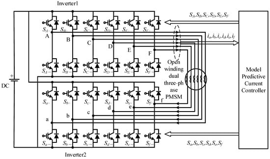
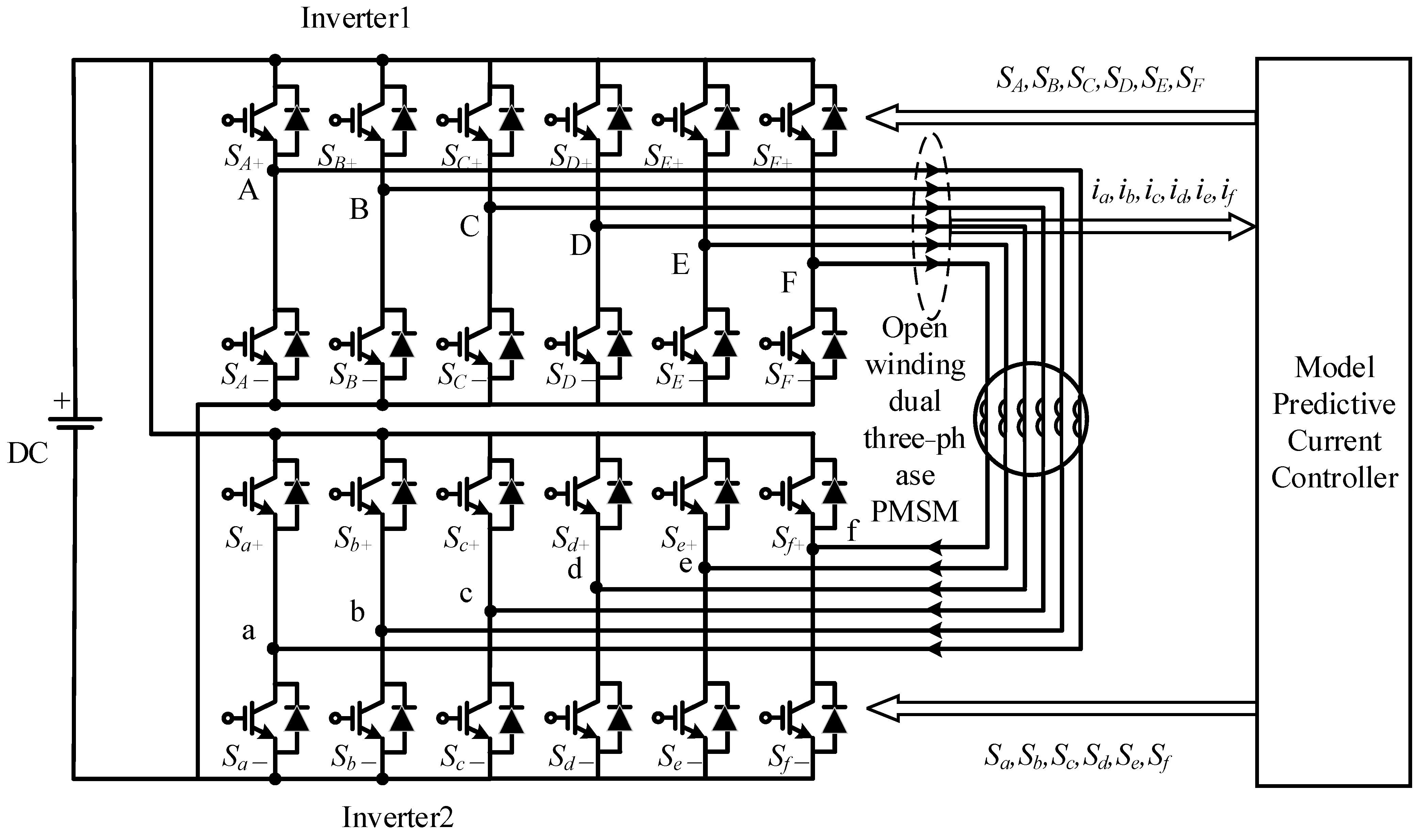
In the common-bus structure, the DC sides of the two inverters share the same DC power supply. The equivalent phase voltage amplitude is higher, DC voltage utilization is significantly improved, and the fault tolerance of the motor is stronger, improving system flexibility and reliability [19,20]. This topology contains common-mode voltage and zero-sequence current loops, so the zero-sequence current should be suppressed as much as possible while the two inverters are driven. In this paper, deadbeat model prediction and IGOMPCC are combined, and the duty-cycle allocation result of inverter 2 is introduced into the cost function equation. This simplifies the calculation, improves the rapidity and accuracy of model prediction, and suppresses harmonic current in the drive system. The topology is shown in Figure 1.

Figure 1. Motor drive system topology.

2.2. Mathematical Model

As shown in Figure 1, each phase of the dual three-phase motor is connected to one bridge arm of an inverter, for a total of six bridge arms. In other words, each motor phase is connected to one inverter leg, resulting in six legs in total. The six phases of inverter 1 are A-F, whereas those of inverter 2 are a-f. Each leg has two power switching devices. In the figure, S represents a power switching device, where the upper leg is denoted by a subscript “+” and the lower leg by a subscript “−”. For example, the upper leg of phase B of inverter 1 is denoted as “S_B+”. Each power switching device has two states: on and off. The upper and lower switching devices of the same leg cannot be on simultaneously. We use [S₁] = {S_A, S_B, S_C, S_D, S_E, S_F} and [S₂] = {S_a, S_b, S_c, S_d, S_e, S_f} to represent the bridge-arm output states of inverters 1 and 2, respectively. Here, S_A, S_B, S_C, S_D, S_E, and S_F represent the switching states of the six legs of inverter 1, and S_a, S_b, S_c, S_d, S_e, and S_f represent those of inverter 2. If the upper leg is on and the lower leg is off, then S = 1; if the upper leg is off and the lower leg is on, then S = 0. Each inverter’s state vector has a total of 26 = 64 switching states.

The stator current of the dual three-phase motor is discretized using the forward Euler method, yielding the discrete-domain stator current equation in three sub-planes, as shown in Equation (1).

$$\left\{\begin{array}{l}{i}_{\alpha }(k+1)=\left(1-{\displaystyle \frac{R_s{T}_s}{L_d}}\right)i_{\alpha }(k)+{\displaystyle \frac{{\omega }_e{\lambda }_f{T}_s\sin \left({\theta }_e\right)}{L_d}}+{\displaystyle \frac{T_s}{L_d}}{u}_{\alpha }(i)\\ i_{\beta }(k+1)=\left(1-{\displaystyle \frac{R_s{T}_s}{L_q}}\right)i_{\beta }(k)-{\displaystyle \frac{{\omega }_e{\lambda }_f{T}_s\cos \left({\theta }_e\right)}{L_q}}+{\displaystyle \frac{T_s}{L_q}}{u}_{\beta }(i)\\ i_{z1}(k+1)=\left(1-{\displaystyle \frac{R_s{T}_s}{L_0}}\right)i_{z1}(k)+{\displaystyle \frac{T_s}{L_0}}{u}_{z1}(i)\\ i_{z2}(k+1)=\left(1-{\displaystyle \frac{R_s{T}_s}{L_0}}\right)i_{z2}(k)+{\displaystyle \frac{T_s}{L_0}}{u}_{z2}(i)\\ i_{o1}(k+1)=\left(1-{\displaystyle \frac{R_s{T}_s}{L_0}}\right)i_{o1}(k)+{\displaystyle \frac{T_s}{L_0}}{u}_{o1}(i)+{\displaystyle \frac{3{\omega }_e{\lambda }_{f3}{T}_s\sin \left(3{\theta }_e\right)}{L_0}}\\ i_{o2}(k+1)=\left(1-{\displaystyle \frac{R_s{T}_s}{L_0}}\right)i_{o2}(k)+{\displaystyle \frac{T_s}{L_0}}{u}_{o2}(i)-{\displaystyle \frac{3{\omega }_e{\lambda }_{f3}{T}_s\cos \left(3{\theta }_e\right)}{L_0}}\end{array}\right.$$

(1)

where i_α(k), i_β(k), i_z1(k), i_z2(k), i_o1(k), and i_o2(k) are the discrete values of the stator current in the three sub-planes; i_α(k + 1), i_β(k + 1), i_z1(k + 1), i_z2(k + 1), i_o1(k + 1), and i_o2(k + 1) are the expected values; u_α(i), u_β(i), u_z1(i), u_z2(i), u_o1(i), and u_o2(i) are the components of the composite voltage vector in the three sub-planes; and T_s is the control period. L_d, L_q, and L₀ are the direct-axis, quadrature-axis, and zero-sequence inductances, respectively; λ_f and λ_f3 are the amplitudes of the fundamental and third-harmonic flux linkages, respectively; R_s is the stator resistance; and ω_e and θ_e are the angular velocity and position angle, respectively.

3. Distribution of Space Voltage Vectors in the Sub-Planes

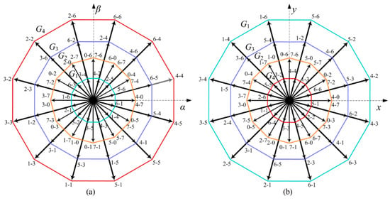
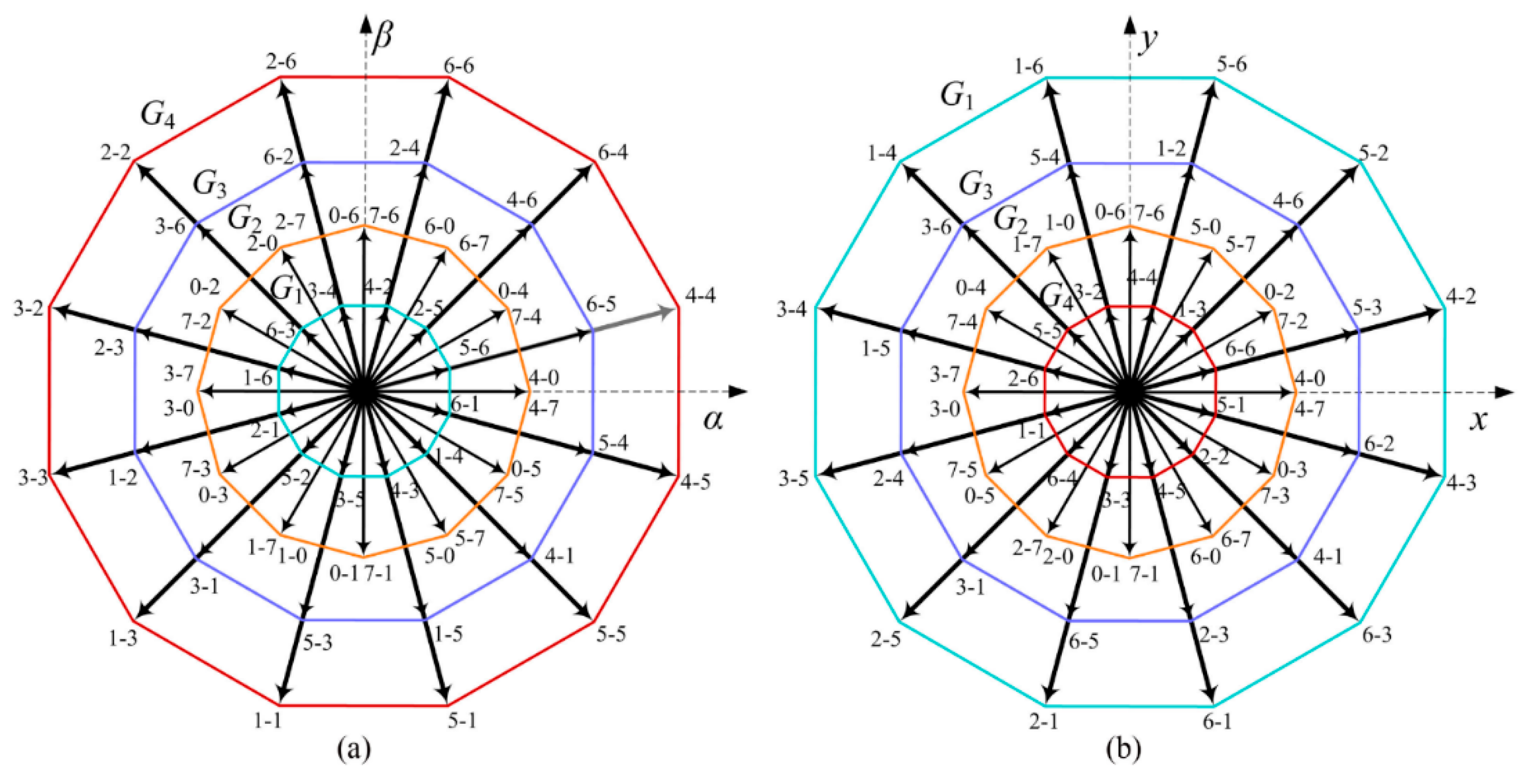
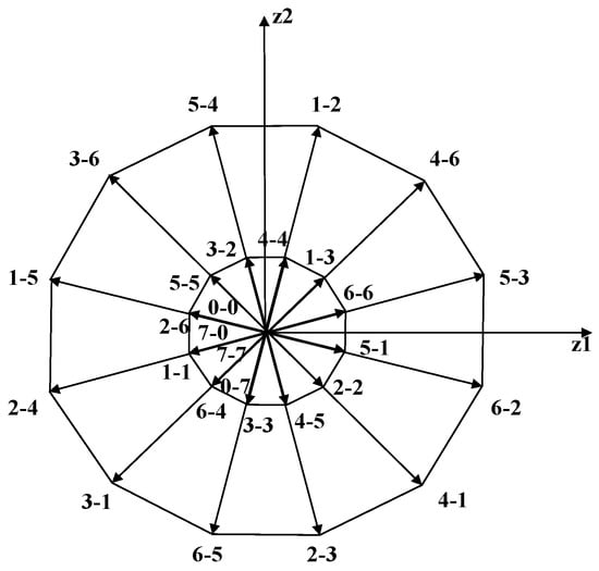
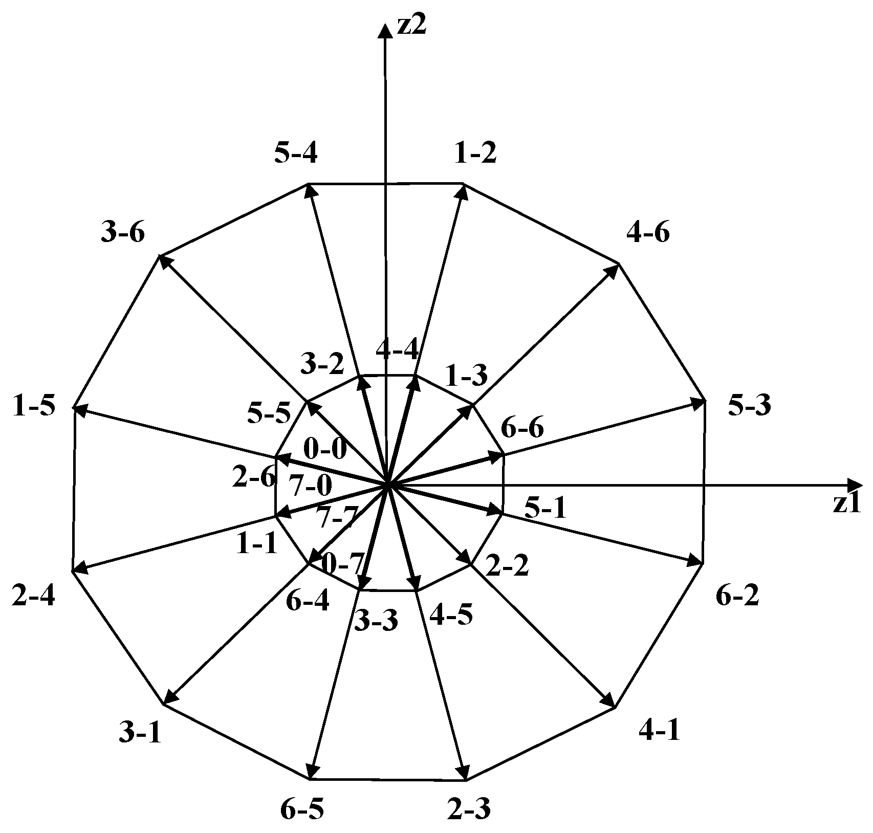
Equations (2) and (3) are the expressions for the space voltage vectors in the α-β and z1-z2 sub-planes, respectively. In these equations, U_dc denotes the DC-side voltage. These voltage-vector equations project the 64 state vectors of the six-phase inverter onto the α-β and z₁-z₂ sub-planes, with v and v_Z representing the spatial voltage vectors of the six-phase inverter in these two sub-planes, respectively.

$$v={\displaystyle \frac{1}{3}}{U}_{\mathrm{dc}}\left(S_A+S_C{e}^{j120}+S_E{e}^{j240}+S_B{e}^{j30}+S_D{e}^{j150}+S_F{e}^{j270}\right)$$

(2)

$$v_Z={\displaystyle \frac{1}{3}}{U}_{\mathrm{dc}}\left(S_A+S_C{e}^{j240}+S_E{e}^{j120}+S_B{e}^{j150}+S_D{e}^{j30}+S_F{e}^{j270}\right)$$

(3)

Based on the voltage-vector distributions described by Equations (2) and (3), we can construct the voltage-vector diagrams for the α-β and z₁-z₂ sub-planes, as illustrated in Figure 2.

Figure 2. Space voltage-vector distribution. (a) α-β sub-planes voltage-vector diagram. (b) z₁-z₂ sub-planes voltage-vector diagram.

For ease of expression, we use “1” to represent the conduction state of the upper bridge arm of the inverter and “0” to represent the conduction state of the lower bridge arm. Because the inverter has six bridge arms, its switching state can be represented by a 6-bit binary number, which is then converted into a 2-digit octal representation. For example, if the upper bridge arms of phases A, D, and E of inverter 1 are conducting and the lower bridge arms of phases B, C, and F are conducting, the current switching state of inverter 1 can be represented by the binary number “100110”. This binary number can then be converted into an octal number and expressed as “4-6”. In Figure 2, all 64 voltage vectors in the α-β and z₁-z₂ sub-planes are represented by octal numbers. As shown in the figure, each sub-plane is composed of four regular dodecagons. Each regular dodecagon has 12 effective voltage vectors: small, medium, medium–large, and large vectors. Therefore, each sub-plane has 48 effective voltage vectors in total. Because each medium vector corresponds to two switching states, the 48 effective voltage vectors correspond to 60 switching states. The output voltage for the “0-0, 0-7, 7-0, 7-7” switching states is zero, corresponding to four zero vectors.

4. IGOMPCC Method

4.1. Control Strategy Block Diagram

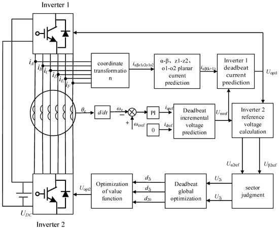
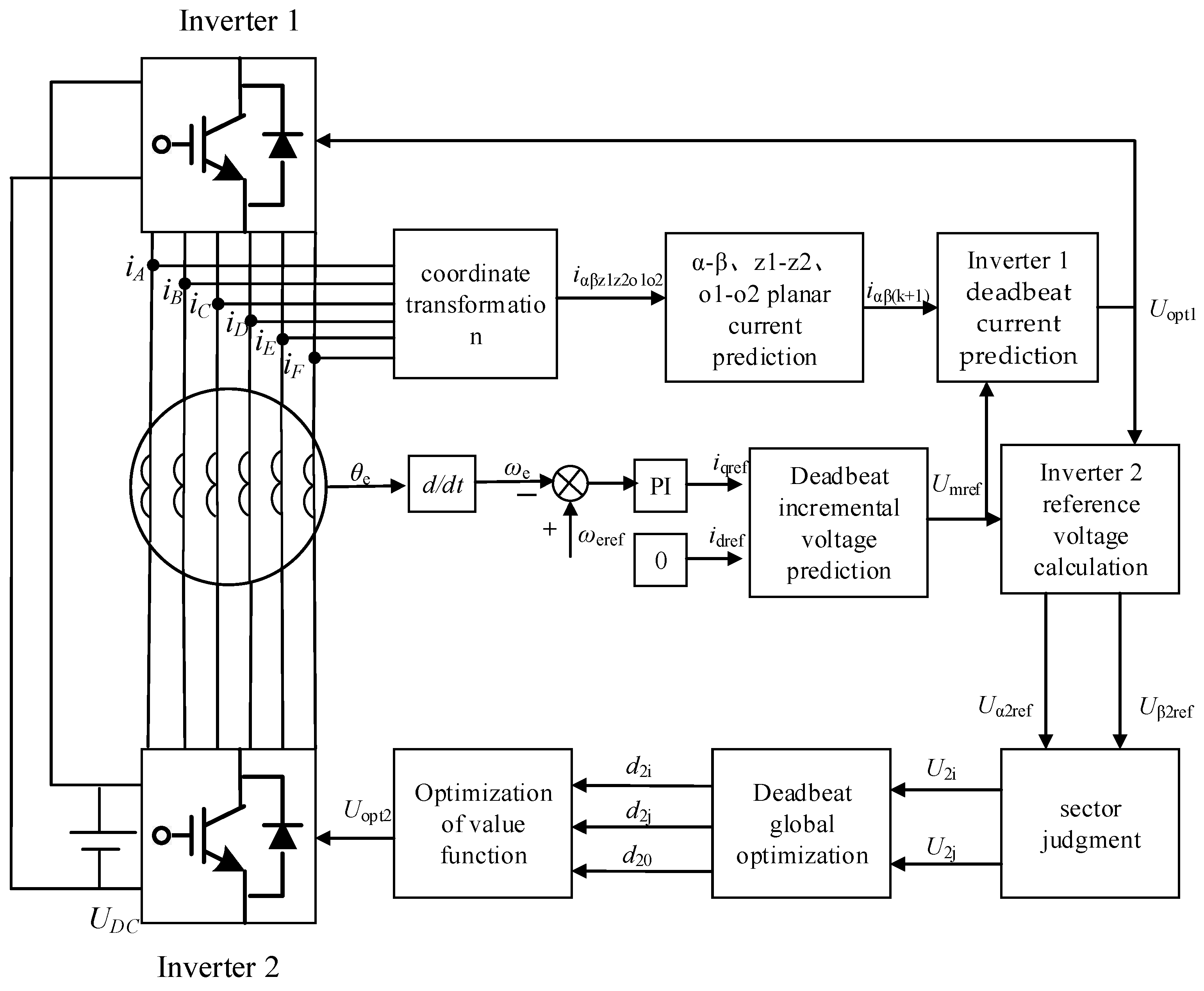
The block diagram of the IGOMPCC method is shown in Figure 3.

Figure 3. IGOMPCC block diagram.

The motor-speed detection module measures and feeds back the rotor angular speed ω_e. The controller obtains the speed error and derives the q-axis reference current i_qref through PI control, while setting i_dref = 0. The α-axis reference current i_αref and the β-axis reference current i_βref in the α-β sub-plane are obtained by inverse rotational coordinate transformation of i_dref and i_qref. Inverter 1 determines the reference voltage in the α-β sub-plane through the deadbeat current predictive control strategy, determines the sector position angle θ_αβ, and then takes the 12 outermost large voltage vectors as the alternative target voltage vectors of inverter 1, which are collectively denoted as U_opt1.

Inverter 2 determines the synthetic voltage vector umref using the deadbeat incremental voltage prediction method and subtracts it from U_opt1 to obtain the α-axis and β-axis reference voltages U_α2ref and U_β2ref of inverter 2. It then determines two groups of alternative target voltage vectors and uses cost function optimization to select the optimal duty-cycle combination. This yields the selected target voltage vector and duty-cycle allocation scheme for inverter 2.

4.2. Control Method for Inverter 1

By performing coordinate transformation on the six-phase current values of inverter 1, we obtain the current values i_α, i_β, i_z1, i_z2, i_o1, and i_o2 of the motor phase currents in the α-β, z₁-z₂, and o₁-o₂ sub-planes. According to the deadbeat current predictive control principle, the forward Euler discretization equation is used to discretize the currents in the three sub-planes, yielding the discrete-time stator currents i_α(k+1) and i_β(k+1). To eliminate the error between the state variable and the reference value at the next time as much as possible, the reference current and voltage values can be used as the expected values.

By decomposing the discrete-domain stator current equation in Equation (1) onto the d–q axes, we can obtain the discretized current prediction equation on the d–q axes in the fundamental-wave space, as shown in Equation (4).

$$\left\{\begin{array}{l}{i}_d(k+1)=(1-{\displaystyle \frac{R_s{T}_s}{L_d}})i_d(k)+{\displaystyle \frac{u_d(k)T_s}{L_d}}+{\displaystyle \frac{T_s}{L_d}}{\omega }_e{L}_q{i}_q(k)\\ i_q(k+1)=(1-{\displaystyle \frac{R_s{T}_s}{L_q}})i_q(k)+{\displaystyle \frac{u_q(k)T_s}{L_q}}-{\displaystyle \frac{T_s}{L_q}}{\omega }_e\left[L_d{i}_d(k)+{\lambda }_f\right]\end{array}\right.$$

(4)

In the equation, i_d(k + 1) and i_q(k + 1) represent the predicted values of stator current in the (k + 1)th control period on the d–q axes, while i_d(k), i_q(k), u_d(k), and u_q(k) denote the discrete-domain components of stator current and voltage in the kth control period on the d–q axes. According to Equation (4), the expression for current in the kth control period can be derived as shown in Equation (5).

$$\left\{\begin{array}{l}{i}_d(k)=(1-{\displaystyle \frac{R_s{T}_s}{L_d}})i_d(k-1)+{\displaystyle \frac{u_d(k-1)T_s}{L_d}}+{\displaystyle \frac{T_s}{L_d}}{\omega }_e{L}_q{i}_q(k-1)\\ i_q(k)=(1-{\displaystyle \frac{R_s{T}_s}{L_q}})i_q(k-1)+{\displaystyle \frac{u_q(k-1)T_s}{L_q}}-{\displaystyle \frac{T_s}{L_q}}{\omega }_e\left[L_d{i}_d(k-1)+{\lambda }_f\right]\end{array}\right.$$

(5)

In the equation, i_d(k − 1), i_q(k − 1), u_d(k − 1), and u_q(k − 1) represent the discrete-domain components of the stator current and voltage on the d–q axes in the (k − 1)th control period. By subtracting Equation (4) from Equation (5), we can obtain the incremental expression of the system as shown in Equations (6)–(9).

$$\left[\begin{array}{l}{i}_d(k+1)-i_d(k)\\ i_q(k+1)-i_q(k)\end{array}\right]=X\left[\begin{array}{l}{i}_d(k)-i_d(k-1)\\ i_q(k)-i_q(k-1)\end{array}\right]+Y\left[\begin{array}{l}{u}_d(k)-u_d(k-1)\\ u_q(k)-u_q(k-1)\end{array}\right]+Z$$

(6)

$$X=\left[\begin{array}{cc}1-{\displaystyle \frac{R_S{T}_S}{L_d}}& {\omega }_e{T}_s\\ -{\omega }_e{T}_s& 1-{\displaystyle \frac{R_S{T}_S}{L_q}}\end{array}\right]$$

(7)

$$Y=\left[\begin{array}{cc}{\displaystyle \frac{T_s}{L_d}}& 0\\ 0& {\displaystyle \frac{T_s}{L_q}}\end{array}\right]$$

(8)

$$Z=\left[\begin{array}{c}0\\ {\displaystyle \frac{-T_s{\lambda }_f}{L_q}}\left[{\omega }_e(k)-{\omega }_e(k-1)\right]\end{array}\right]$$

(9)

Over the interval from the k-th to the (k + 1)th control period, the rotor-speed change can be neglected, so the matrix Z in Equation (9) can be approximated as 0. By using i_d(k + 1) and i_q(k + 1) from the (k + 1)th control period as the reference currents i_dref and i_qref, the incremental voltage reference vector on the d–q axes is obtained, as shown in Equation (10).

$$\left\{\begin{array}{c}{u}_{\mathit{dref}}=u_d(k-1)+{\displaystyle \frac{L_d}{T_s}}[i_{\mathit{dref}}-i_d(k)(2-{\displaystyle \frac{T_s{R}_s}{L_d}})+\\ i_d(k-1)(1-{\displaystyle \frac{T_s{R}_s}{L_d}})]-{\omega }_e{L}_d\left[i_q(k)-i_q(k-1)\right]\\ u_{\mathit{qref}}=u_q(k-1)+{\displaystyle \frac{L_d}{T_s}}[i_{\mathit{qref}}-i_q(k)(2-{\displaystyle \frac{T_s{R}_s}{L_d}})+\\ i_q(k-1)(1-{\displaystyle \frac{T_s{R}_s}{L_d}})]-{\omega }_e{L}_d\left[i_d(k)-i_d(k-1)\right]\end{array}\right.$$

(10)

The incremental voltage reference vector on the d–q axes is transformed into the α-β sub-plane to obtain the voltage reference values u_αref and u_βref at time k. Finally, the sector position angle θ_αβ of U_opt1 is calculated using Equation (11).

$${\theta }_{\mathit{\alpha \beta }}=\arctan {\displaystyle \frac{u_{\mathit{\beta ref}}}{u_{\mathit{\alpha ref}}}}$$

(11)

To maximize voltage utilization, simplify the deadbeat model prediction calculation, and reduce time delay, we select the 12 large vectors of inverter 1 as alternative target voltage vectors and determine the target sector and U_opt1 using Equation (11).

4.3. Control Method for Inverter 2

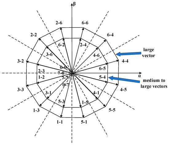
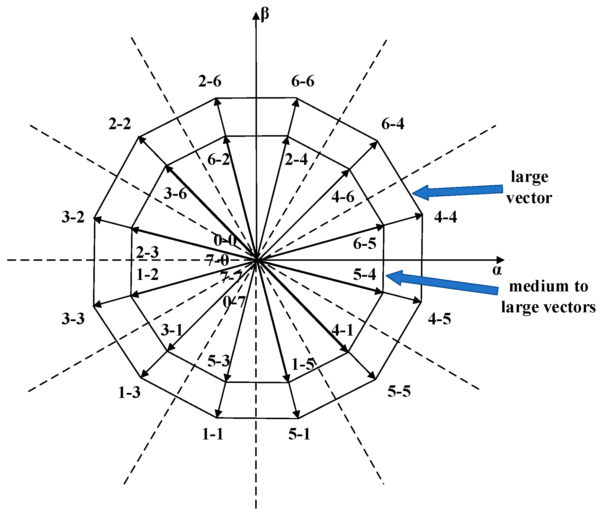
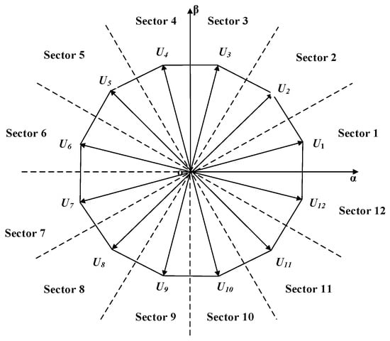
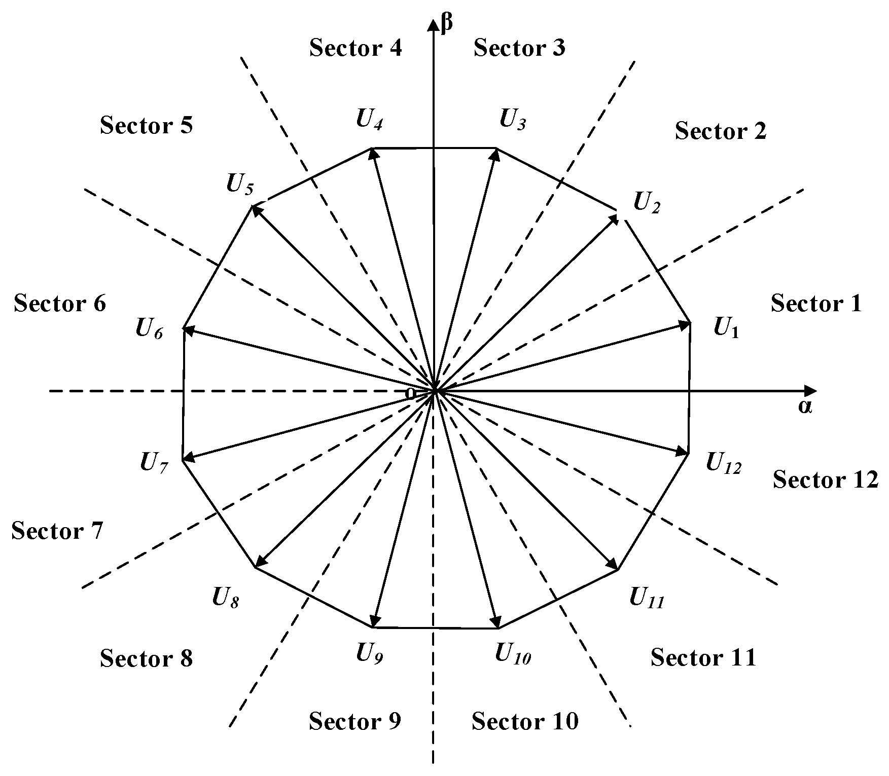
Figure 4 and Figure 5 show the distributions of medium and large vectors in the α-β and z₁-z₂ sub-planes, respectively. As shown in the figures, the outermost large vector and the second outermost medium–large vector in the α-β sub-plane correspond to small and medium–large vectors in the z₁-z₂ sub-plane, and the phase difference between the small and medium–large vectors is 180°.

Figure 4. Distribution of medium–large and large vectors in the α-β sub-plane.

Figure 5. Distribution of medium–large and large vectors in the z₁-z₂ sub-plane.

Using this characteristic, we can simply control the proportions of the medium–large, large, and zero vectors according to the proportional relationship in Equation (12), so that the synthesized vector approaches 0 in the z1-z2 sub-plane, thereby suppressing harmonic currents.

U_Z = 0.268U_ML + 0.732U_L

(12)

In the equation, U_Z represents the alternative composite voltage vector, U_ML represents the alternative medium-to-large voltage vector, and U_L represents the alternative large voltage vector. Twelve alternative vector groups can synthesize twelve alternative composite voltage vectors U_Z, and the distribution of these alternative composite voltage vectors is shown in Figure 6.

Figure 6. Distribution of alternative synthetic voltage vector U_Z.

According to Equation (13), the reference voltage components U_α2ref and U_β2ref of inverter 2 are obtained.

$$\begin{array}{l}\left\{\begin{array}{c}{u}_{\alpha 2\mathit{ref}}=u_{\alpha 1-\mathit{opt}}-u_{\mathit{\alpha ref}}\\ u_{\beta 2\mathit{ref}}=u_{\beta 1-\mathit{opt}}-u_{\mathit{\beta ref}}\end{array}\right.\\ \end{array}$$

(13)

Using Equation (11), the sector position angle θ_αβ2 of the reference voltage vector of inverter 2 can be calculated, and the alternative reference voltage vectors can be determined from Figure 6. Taking θ_αβ2 = 135° as an example, there are two groups of alternative reference voltage vectors: the U₄ and U₅ vector group and the U₆ and U₅ vector group. Using Equation (14) as the cost function and requiring the sum of all duty cycles within a control period to be 1, the minimum value of the cost function is calculated under the constraints of Equation (15) to ultimately determine the optimal duty cycle.

$$J(u_m)={[i_{\mathit{dref}}-i_{\mathit{dm}}(k+1)]}^2+{[i_{\mathit{qref}}-i_{\mathit{qm}}(k+1)]}^2$$

(14)

d_i + d_j + d₀ = 1

(15)

In the equation, i_dm(k + 1) and i_qm(k + 1) represent the predicted current values of the synthesized voltage vector of inverter 2 on the d–q axes, and d₀ is the duty cycle of the zero vector. By assigning duty cycles to the candidate reference voltage-vector group, the synthesized voltage vector U_opt2 of inverter 2 is obtained as shown in Equation (16).

u_opt2 = d_iu_2i + d_ju_2j

(16)

Here, u_opt2 represents the synthesized voltage vector of inverter 2; u_2i and u_2j are two alternative voltage vectors in the alternative reference voltage-vector group; and d_i and d_j are the duty cycles assigned to these two alternative voltage vectors, respectively.

5. Simulation Results and Analysis

The effectiveness of IGOMPCC was verified through MATLAB R2024a simulations, and the motor parameters are listed in Table 1.

Table 1. Parameters of the simulated motor.

Element	Parameter
resistance Rs	0.65 Ω
direct-axis inductance Ld	2.47 mH
quadrature-axis inductance Lq	2.47 mH
zero-sequence inductance L0	0.5 mH
fundamental flux linkage λf	0.0885 Wb
Number of pole pairs, p	5

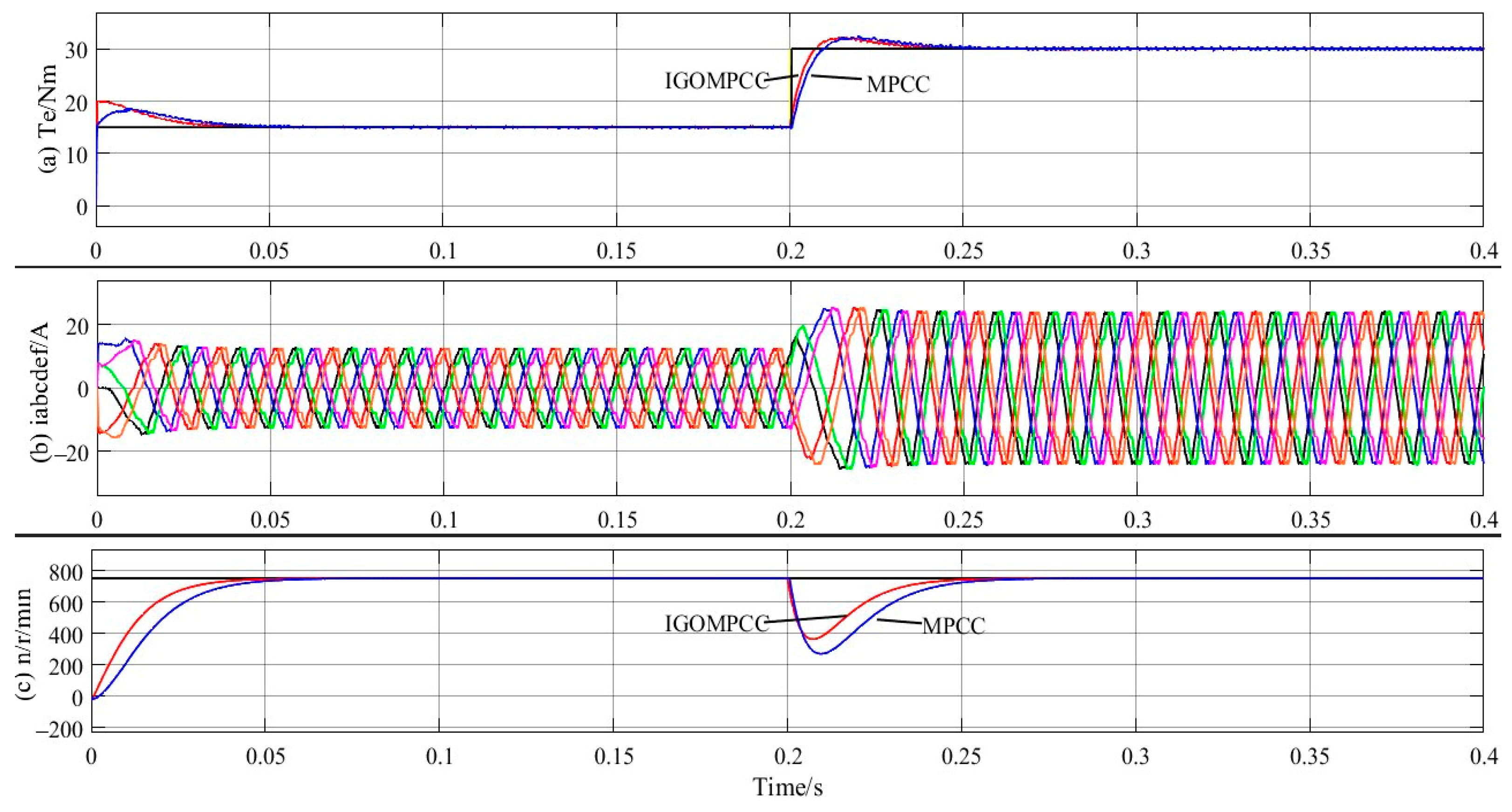
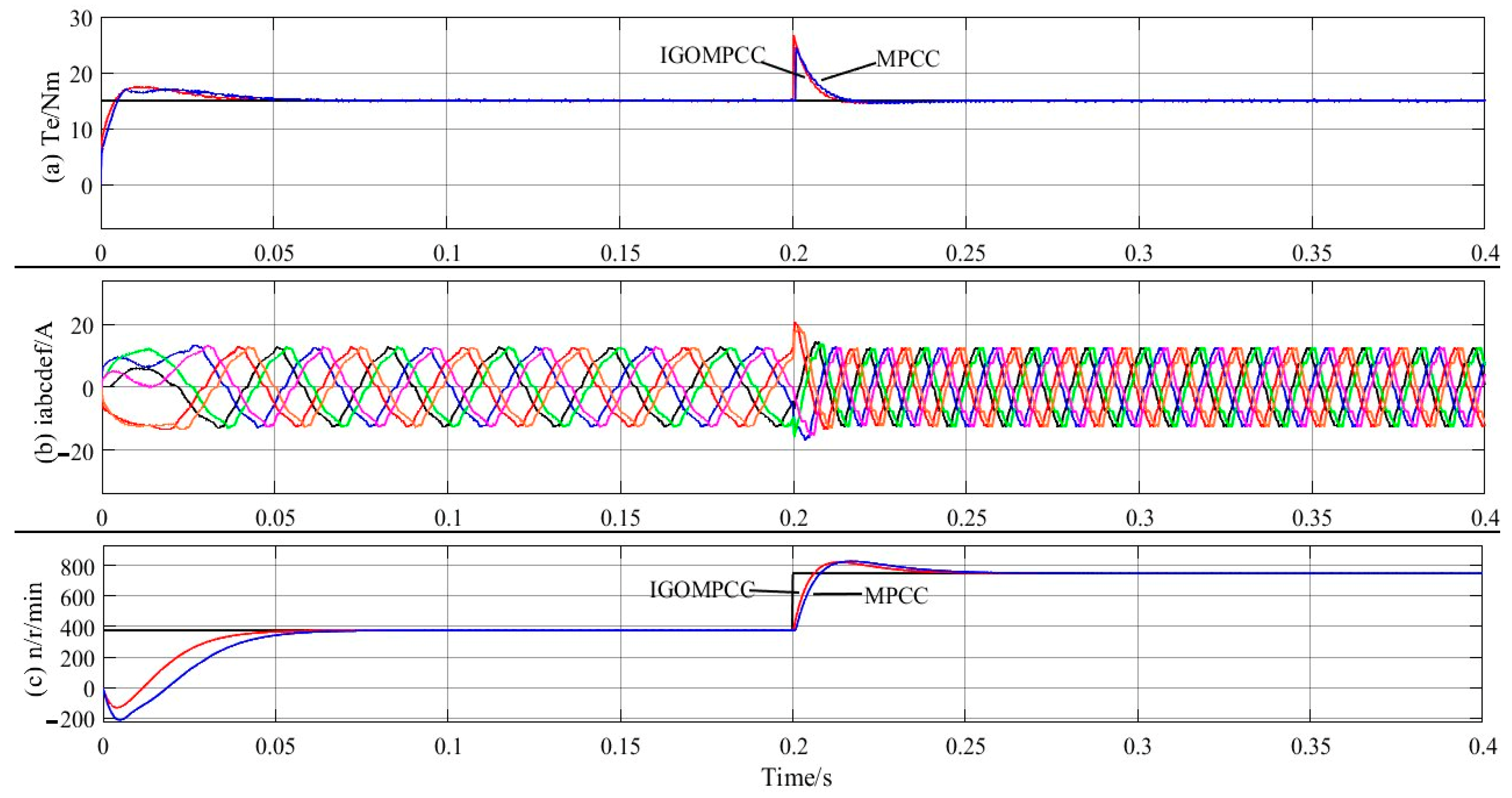
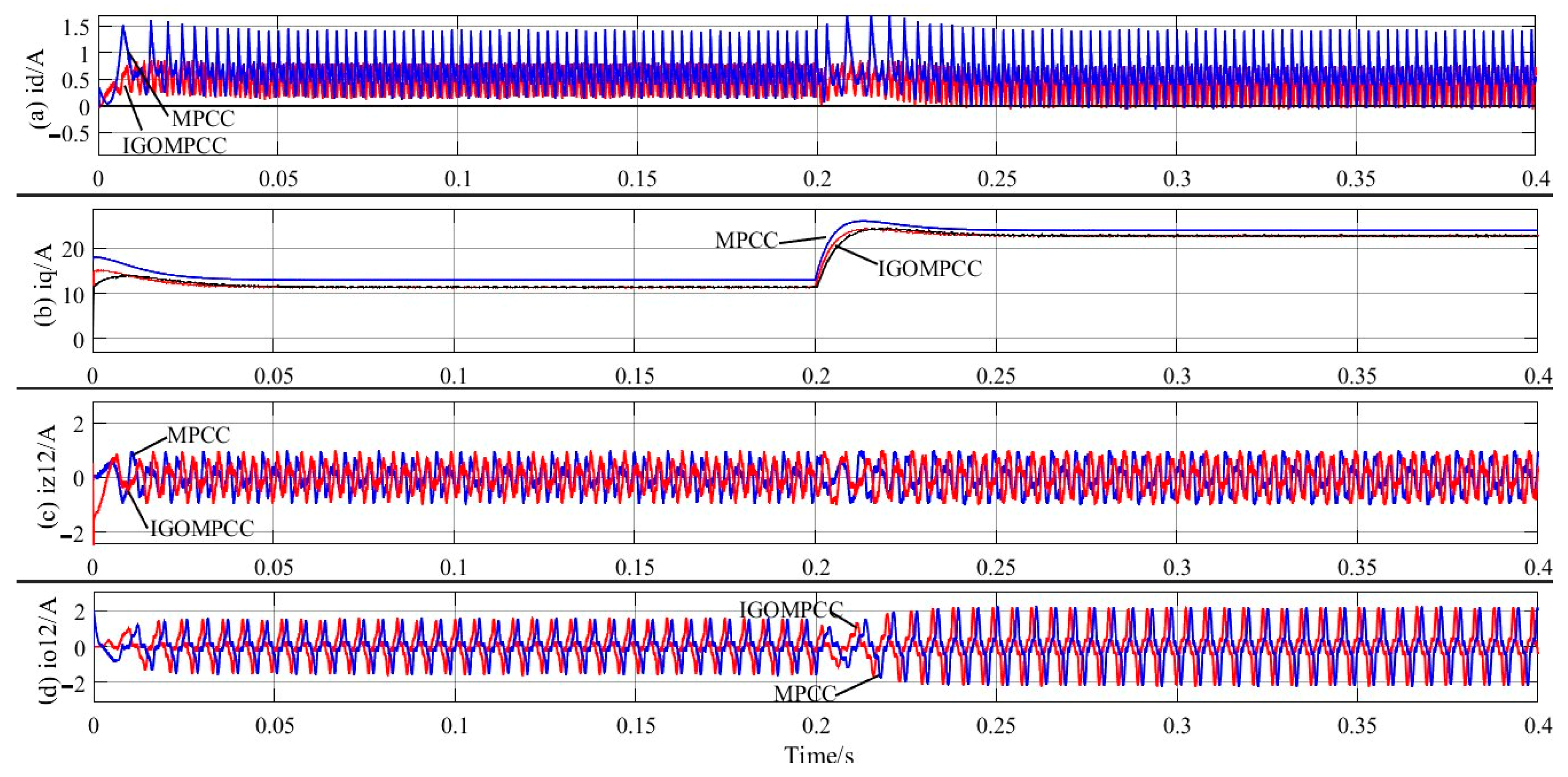
In the simulation waveform diagram, the reference value is represented by the black line, the simulation waveform of traditional MPCC by the blue line, and the simulation waveform of IGOMPCC by the red line.

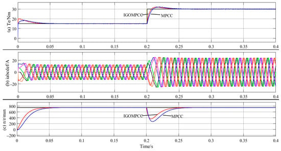
Figure 7 shows the simulated waveforms when the load torque steps from 15 Nm to 30 Nm at 0.2 s. At the instant of the sudden increase, the q-axis current reference rises immediately, and the electromagnetic torque and stator phase-current amplitude of both methods increase; the phase-current amplitude increases from 13 A to 27 A. The dynamic processes, however, differ significantly. The electromagnetic torque of traditional MPCC requires 50 ms to stabilize at 30 Nm, and the speed drops to 285 r/min. It then recovers to 750 r/min in about 0.25 s. The electromagnetic torque of IGOMPCC follows its target within 40 ms, which shortens the adjustment time by 20%; the speed drops to 360 r/min, and the speed recovers to 750 r/min in 0.24 s.

Figure 7. Waveform of torque, current, and speed at sudden torque increase.

The reason for this difference lies in the different control delays. After a sudden load change, inverter 1 of IGOMPCC directly calculates the fundamental reference voltage using a deadbeat equation and locks onto the outermost large vector. Inverter 2 solves the duty cycle within two sets of candidate voltage vectors using the Lagrange multiplier method, reducing the number of single-cycle cost function evaluations from 144 to 3 and allowing the reference voltage to be reconstructed within the current control period. Traditional MPCC requires current prediction and cost function comparison for all candidate vectors within one period, and the time spent on rolling optimization delays its voltage update, resulting in a slower torque response.

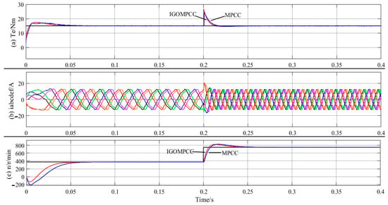
Figure 8 depicts the simulated waveform obtained when the reference speed changes from 380 r/min to 750 r/min at 0.2 s, corresponding to an increase in stator electrical frequency from 31.7 Hz to 62.5 Hz. As shown in the figure, the IGOMPCC speed adjustment is completed within 27 ms, with an overshoot of 6.7%; in contrast, traditional MPCC takes 41 ms, with an overshoot of 8%, corresponding to a 34.1% reduction in adjustment time. In terms of average acceleration, the value increases from approximately 9.0 × 10³ r/min/s to approximately 1.37 × 10⁴ r/min/s, which is an improvement of about 52%.

Figure 8. Waveform of torque, stator current, and speed at sudden speed increase.

The ability of IGOMPCC to output a larger acceleration torque has two causes. First, inverter 1 always selects the outermost 12 large vectors during the dynamic phase, maximizing the utilization of the DC-bus voltage and providing a larger voltage margin for the q-axis current. Second, incremental prediction does not rely on the flux-linkage parameter λ_f. Even if the flux-linkage operating point changes during acceleration, the reference voltage solution remains consistent with the actual object, allowing the q-axis current to track the reference value given by the outer speed loop quickly. In contrast, the q-axis current of traditional MPCC has a significant steady-state error, limiting the continuous growth of acceleration torque. Notably, during the rapid increase in electrical frequency from 31.7 Hz to 62.5 Hz, the phase-current waveform of IGOMPCC maintains good sinusoidal quality, indicating that speed changes do not weaken its suppression capability in the harmonic sub-plane.

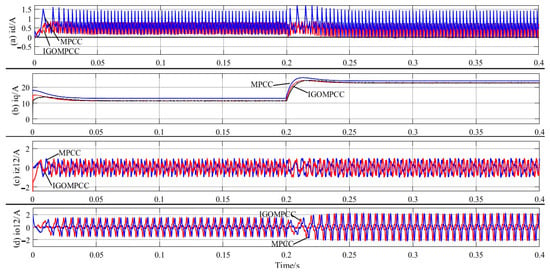
Figure 9 shows that the d-axis current fluctuation under IGOMPCC is smaller and closer to the reference value of 0. In the q-axis current waveform, the q-axis current of IGOMPCC almost coincides with the reference value, whereas the q-axis current of traditional MPCC has a significant steady-state error relative to the reference. We abruptly increased the load torque from 15 Nm to 30 Nm at 0.2 s. During this sudden increase, the peak d-axis current fluctuation under IGOMPCC was only 0.8 A, a 52.9% decrease compared with the 1.7 A under traditional MPCC. This indicates a higher degree of decoupling between the fundamental and harmonic sub-planes, preventing load disturbances from being amplified through d–q axis coupling. The q-axis current of IGOMPCC approaches the reference value more quickly and accurately during a sudden torque increase, indicating that IGOMPCC can effectively suppress stator current harmonics and reduce torque ripple. The q-axis current responds more sensitively to a sudden load-torque change: the load torque increases abruptly, and the electromagnetic torque rises rapidly, demonstrating the good dynamic performance of the IGOMPCC method.

Figure 9. Current waveforms of the motor in the d-q axes, z₁-z₂ sub-plane, and o₁-o₂ sub-plane.

Figure 9c,d depict the current waveforms in the z₁-z₂ and o₁-o₂ sub-planes, respectively. In the z₁-z₂ sub-plane, i_z1 and i_z2 under IGOMPCC are suppressed within ±0.98 A, whereas the fluctuation amplitude of i_z1 and i_z2 under traditional MPCC reaches ±1.1 A, representing a decrease of approximately 10.9% for the former relative to the latter. The fundamental difference between the two methods lies in their harmonic-suppression mechanisms. IGOMPCC uses the distribution characteristic of large and medium–large vectors with a phase difference of 180° in the z₁-z₂ sub-plane to pre-synthesize candidate vectors at a fixed ratio of 0.268:0.732 according to Equation (12), ensuring that the synthesized voltage in the harmonic sub-plane structurally approaches zero and thereby eliminating the voltage excitation for harmonic-current generation. Traditional MPCC relies on the harmonic-sub-plane penalty term in the cost function to suppress harmonics. However, this weight requires empirical tuning, and the method is limited to a single vector output per cycle. This permits only a compromise selection from a finite set of vectors and prevents precise cancelation of the harmonic voltage. Consequently, significant harmonic current persists in the z₁-z₂ sub-plane. This is the fundamental reason why IGOMPCC exhibits lower total harmonic distortion of the stator current and smaller torque ripple.

The amplitudes of i_o1 and i_o2 are basically equivalent for both methods: ±1.8 A before the sudden torque increase and ±2.1 A after the sudden torque increase has stabilized. It should be noted that the vector pre-synthesis of IGOMPCC is designed mainly for the z₁-z₂ sub-plane, and the o₁-o₂ components are not included in the cost function, so no special constraints are imposed on the zero-sequence sub-plane. The amplitude of the third-harmonic flux linkage in this simulation system is relatively small, and the overall zero-sequence current level is low, which does not substantially affect control performance. This is one limitation of the proposed method, and future work will introduce zero-sequence component constraints into the cost function.

6. Conclusions

In this paper, an IGOMPCC strategy is proposed. Inverter 1 uses the deadbeat model predictive current control method, and inverter 2 uses the deadbeat method to determine the alternative target-vector group. The optimal global optimization scheme is then determined after duty-cycle allocation by calculating the minimum cost function. Through simulation analysis, the control performance of IGOMPCC and traditional MPCC is compared. Table 2 compares computational complexity and algorithm structure, whereas Table 3 compares dynamic and static performance between IGOMPCC and traditional MPCC.

Table 2. Comparison of computational complexity and algorithm structure between IGOMPCC and traditional MPCC.

Comparison Item	Traditional MPCC	IGOMPCC	Improvement
Number of candidate switching combinations per cycle	144	3	Decreased by 97.9%
Number of cost function evaluations	144	3	Decreased by 97.9%
Duty-cycle solution method	Traverse rolling optimization	Lagrange multiplier method	Transforms optimization into a closed-form solution, reducing the number of optimization iterations
Dependence of the prediction model on flux linkage λf	Dependent on λf	Independent of λf	Eliminates dependence on flux linkage, enhancing robustness
z1–z2 harmonic suppression	Relies on empirical tuning of harmonic-term weights in the cost function	The synthesized vector harmonic voltage approaches 0	Eliminates tuning and achieves more thorough harmonic suppression
Equivalent switching frequency	Not fixed	Fixed by selecting adjacent vectors for duty-cycle modulation	Beneficial for filter design

Table 3. Quantitative comparison of dynamic and static performance between IGOMPCC and traditional MPCC.

Performance Indicator	Test Condition	Traditional MPCC	IGOMPCC	Improvement
Regulation time for sudden torque increase	15 N·m to 30 N·m	50 ms	40 ms	Regulation time reduced by 20%
Speed drop during sudden torque increase	15 N·m to 30 N·m	285 r/min	360 r/min	Speed drop is reduced by 10%
Overshoot during sudden speed increase	380 r/min to 750 r/min	8%	6.7%	Overshoot decreased by 1.3 percentage points
Regulation time for sudden increase in speed	380 r/min to 750 r/min	41 ms	27 ms	Regulation time reduced by 34.1%
Peak d-axis current fluctuation during sudden torque increase	15 N·m to 30 N·m	1.7 A	0.8 A	Peak fluctuation decreased by 52.9%
Steady-state static error of q-axis current during sudden torque increase	15 N·m to 30 N·m	2.7 A	approaches 0	Eliminates steady-state error in the q-axis current

The main conclusions are as follows:

• Combining deadbeat control, incremental global optimization, and cost function-based rolling allocation of the optimal duty cycle can minimize the number of candidate target-vector groups, reducing the number of cost function evaluations by 97.9%. Using the Lagrange multiplier method for duty-cycle rolling optimization can significantly reduce the processor’s computational load and complexity, enhancing the system’s response speed.
• The electromagnetic torque under IGOMPCC can track changes in load torque more sensitively, with smaller speed fluctuations and a 20% reduction in adjustment time. When the reference speed increases suddenly, the motor using IGOMPCC can achieve greater acceleration, with a 34.1% reduction in adjustment time and a 1.3% decrease in speed overshoot. In addition, the total harmonic distortion of the stator current is low, indicating better dynamic performance under IGOMPCC.
• The steady-state error of the q-axis current under IGOMPCC approaches 0. When the load torque increases suddenly, the peak d-axis current fluctuation decreases by 52.9%, and the q-axis current increases faster, indicating that IGOMPCC provides more sensitive dq-axis current control and lower stator current harmonic content.
• IGOMPCC does not require the motor’s flux-linkage parameters when calculating the voltage reference vector of the predictive model. Therefore, it can achieve zero steady-state error tracking of the q-axis current reference even under mismatch in motor flux-linkage parameters, enhancing the robustness of dual three-phase open-winding permanent-magnet motor control.
• Unlike traditional MPCC, in which a single vector acts during each cycle and switches randomly according to operating conditions, IGOMPCC synthesizes two adjacent effective vectors and a zero vector on the inverter 2 side according to an analytical duty cycle, while inverter 1 directly locks onto the sector’s large vector without rolling optimization. Because the vector sets are limited, the duty cycle is solved using the Lagrange multiplier method to eliminate optimization delay jitter. The switching instants can be predetermined, forming a fixed equivalent switching frequency that concentrates harmonics near the switching frequency rather than dispersing them over a wide band. This facilitates filter design and reduces ripple and torque ripple under the same loss.

References

- Cui, R.; Fan, Y.; Cheng, M. A new zero-sequence current suppression control strategy for five-phase open-winding fault-tolerant fractional-slot concentrated winding IPM motor driving system. IEEE Trans. Ind. Appl. 2019, 55, 2731–2740. [Google Scholar] [CrossRef] [Scilit]
- Yin, Z.; Sui, Y.; Xing, L.; Zheng, P.; Cheng, L.; Liu, J. Comparative investigations of inverter short-circuit fault and winding terminal short-circuit fault in open-end winding five-phase PM machine system. IEEE Trans. Magn. 2021, 57, 8106705. [Google Scholar] [CrossRef] [Scilit]
- Luo, Y.; Liu, C. Elimination of harmonic currents using a reference voltage vector based-model predictive control for a six-phase PMSM motor. IEEE Trans. Power Electron. 2019, 34, 6960–6972. [Google Scholar] [CrossRef] [Scilit]
- Zoric, I.; Jones, M.; Levi, E. Arbitrary power sharing among three-phase winding sets of multiphase machines. IEEE Trans. Ind. Electron. 2018, 65, 1128–1139. [Google Scholar] [CrossRef] [Scilit]
- Luo, Y.; Liu, C. Model predictive control for a six-phase PMSM motor with a reduced-dimension cost function. IEEE Trans. Ind. Electron. 2020, 67, 969–979. [Google Scholar] [CrossRef] [Scilit]
- Liu, S.; Liu, C.; Huang, Y.; Xiao, Y. Direct modulation pattern control for dual three-phase PMSM drive system. IEEE Trans. Ind. Electron. 2022, 69, 110–120. [Google Scholar] [CrossRef] [Scilit]
- Ayala, M.; Doval-Gandoy, J.; Gonzalez, O.; Rodas, J.; Gregor, R.; Rivera, M. Experimental stability study of modulated model predictive current controllers applied to six-phase induction motor drives. IEEE Trans. Power Electron. 2021, 36, 13275–13284. [Google Scholar] [CrossRef] [Scilit]
- Liu, J.; Zhang, B.; Feng, W.; Zhao, G. Model predictive current control for open-winding PMSM with non-common bus dual inverter power supply. Electr. Mach. Control Appl. 2025, 52, 1137–1147. (In Chinese) [Google Scholar] [CrossRef]
- Gonçalves, P.F.C.; Cruz, S.M.A.; Mendes, A.M.S. Multistage predictive current control based on virtual vectors for the reduction of current harmonics in six-phase PMSMs. IEEE Trans. Energy Convers. 2021, 36, 1368–1377. [Google Scholar] [CrossRef] [Scilit]
- Ayala, M.; Doval-Gandoy, J.; Rodas, J.; Gonzalez, O.; Gregor, R.; Rivera, M. A novel modulated model predictive control applied to six-phase induction motor drives. IEEE Trans. Ind. Electron. 2021, 68, 3672–3682. [Google Scholar] [CrossRef] [Scilit]
- Zhang, C.; Wang, H.; Shen, H.; Wu, X. Improved model predictive torque control for nine-phase open-end winding permanent magnet synchronous motors. Proc. Chin. Soc. Electr. Eng. 2026, 46, 6961–6970. (In Chinese) [Google Scholar] [CrossRef]
- Mavila, P.C.; Rajeevan, P.P.; Rajeevan, R. A five-level torque controller based DTC scheme for open-end winding five-phase IM drives with single DC source and auxiliary plane harmonic elimination. IEEE Trans. Ind. Appl. 2022, 58, 2063–2074. [Google Scholar] [CrossRef] [Scilit]
- Peng, Y.; Sun, C.; Yuan, W.; Gong, J.; Huang, M.; Zha, X. Deadbeat predictive torque control of six-phase open-end winding PMSM based on harmonic plane decomposition and voltage vector constraints. Proc. Chin. Soc. Electr. Eng. 2026, 46, 4735–4745. (In Chinese) [Google Scholar] [CrossRef]
- Wang, W.; Liu, C.; Liu, S.; Zhao, H. Model predictive torque control for dual three-phase PMSMs with simplified deadbeat solution and discrete space-vector modulation. IEEE Trans. Energy Convers. 2021, 36, 1491–1499. [Google Scholar] [CrossRef] [Scilit]
- Yan, L.; Zhu, Z.-Q.; Qi, J.; Ren, Y.; Gan, C.; Brockway, S.; Hilton, C. Enhancement of disturbance rejection capability in dual three-phase PMSM system by using virtual impedance. IEEE Trans. Ind. Appl. 2021, 57, 4901–4912. [Google Scholar] [CrossRef] [Scilit]
- Xie, N.; Xiao, L.; Wu, Q.; Wang, Q. Model predictive current control of dual three-phase PMSM based on incremental global optimization. Power Electron. 2026, 60, 129–136. (In Chinese) [Google Scholar] [CrossRef]
- Sha, O.; Tang, H. Research on an improved deadbeat model predictive current control of double three-phase open-winding permanent magnet motor. J. Vibroeng. 2024, 26, 1791–1805. [Google Scholar] [CrossRef] [Scilit]
- Chen, Y.; Zhang, B.; Zhao, G.; Niu, S.; Hou, Y.; Liu, C. An optimized modulation strategy for four-leg VSI-fed dual three-phase PMSM drives considering capacitor voltage fluctuation. IEEE Trans. Power Electron. 2026; in press. [CrossRef] [Scilit]
- Li, X.; Zhang, S.; Zhang, C.; Zhou, Y.; Yuan, X.; Dong, Y. Model predictive control with duty ratio modulation for open-winding PMSM drives with common DC bus. IEEE Trans. Power Electron. 2023, 38, 15287–15299. [Google Scholar] [CrossRef] [Scilit]
- Mousavi, M.S.; Davari, S.A.; Nekoukar, V.; Garcia, C.; Rodriguez, J. Computationally efficient model-free predictive control of zero-sequence current in dual inverter fed induction motor. IEEE J. Emerg. Sel. Top. Power Electron. 2023, 11, 1332–1344. [Google Scholar] [CrossRef] [Scilit]
Disclaimer/Publisher’s Note: The statements, opinions and data contained in all publications are solely those of the individual author(s) and contributor(s) and not of MDPI and/or the editor(s). MDPI and/or the editor(s) disclaim responsibility for any injury to people or property resulting from any ideas, methods, instructions or products referred to in the content. |
© 2026 by the authors. Licensee MDPI, Basel, Switzerland. This article is an open access article distributed under the terms and conditions of the Creative Commons Attribution (CC BY) license.