Indoor Positioning Method Based on Multi-Objective Semantic Structure Inference of WiFi FTM

Abstract

WiFi Fine Timing Measurement (FTM) directly provides round-trip delay ranging information between a mobile terminal and an access point (AP), serving as a critical technical foundation for the development of low-cost indoor positioning systems. However, indoor wall occlusion, multipath propagation, and intermittent link outages introduce spatially correlated systematic biases into FTM ranging measurements, rendering traditional multilateration methods vulnerable to abnormal observation outliers. To address this issue, this paper proposes an indoor positioning algorithm based on multi-objective semantic structure inference for WiFi FTM. Given available FTM ranging values, measurement masks, timestamps, and known AP coordinates, the proposed method first constructs FTM feature labels using AP distance vectors, distance differentials, and time differentials. Subsequently, wireless semantic embeddings are obtained by modeling masked AP distance measurements and implementing temporal-proximity contrastive learning. The implicit latent states derived from embedding clustering are interpreted as typical ranging pattern states, and state-dependent AP ranging biases are adopted to characterize non-line-of-sight (NLOS) errors under diverse spatial topographies. A semantic field and state transition matrix are further employed to model the spatial distribution and temporal adjacency relationships of these ranging states. Finally, by alternately optimizing a composite objective function consisting of Student-t mixture likelihood, FTM differential constraints, and link reliability constraints, the terminal position is estimated in a joint and robust manner. Experiments show that the mean error of this algorithm is 0.66 m, the median error is 0.64 m, and the 90th percentile error is 0.90 m. Compared with the conventional FTM least-squares multilateration baseline, the proposed method reduces the RMSE and mean error by 72.27% and 60.77%, respectively. Compared with the best conventional baseline (PSO), the corresponding reductions are 36.65% and 28.4%. These results indicate that visibility, relative distance, and residual variations within the FTM sequence can form useful implicit topological constraints for localization. These absolute accuracies are specific to the tested experimental setup. The relative improvements are reported to indicate the gain over conventional methods.

1. Introduction

Indoor positioning is a core enabling technology for smart buildings, warehouse logistics, industrial automation, and augmented reality services. Satellite navigation suffers from severe signal attenuation indoors. In contrast, WiFi infrastructure is widely deployed and can provide ranging and fingerprint observations without the need for dedicated hardware [1,2]. Among WiFi measurements, FTM can provide round-trip time ranging at meter-level or higher accuracy. Received Signal Strength Indicator (RSSI) has the advantages of high energy efficiency and universal availability [3,4].

Early systems relied on trilateration using FTM distances or utilized RSSI fingerprint matching [5,6]. These methods are simple and highly interpretable, but their performance often degrades in complex indoor environments. This is because single measurement modalities capture only partial physical information. The AP positions are usually assumed to be known or calibrated through offline means. Recent studies have improved positioning accuracy by integrating FTM [7,8], RSSI [9,10], and inertial measurements [11,12] into optimization algorithms. However, they neglect the semantic structure of the indoor environment [13,14].

In the past few years, WiFi sensing has progressively expanded from simple presence detection and action recognition to tasks such as gesture recognition, human identity recognition, health monitoring, environmental perception, and semantic understanding [15,16]. WiFi signals are highly environment-dependent. Changes in room layouts, AP placements, human poses, and device configurations can cause signal distribution variations. Therefore, extracting high-level semantics that are both interpretable and transferable from unstable low-level radio signals has become a critical issue for the further development of WiFi sensing.

Semantic localization constrains the search space using understandable areas such as corridors, laboratories, offices, and foyers, while maintaining maps with temporal significance [17,18]. Semantic communication research provides a higher theoretical background for WiFi semantic mapping. Traditional communication systems primarily focus on bit-level reliable transmission, whereas semantic communication emphasizes the meaning, task relevance, and reception understanding of transmitted information. Related reviews point out that the core of semantic communication lies in extracting and transmitting the “meaning” within data, relying on a shared or aligned knowledge base between the transmitter and receiver to achieve semantic interpretation [19,20].

This paper proposes an indoor positioning algorithm based on multi-objective semantic structure inference of WiFi FTM. The main contributions of this work are as follows:

• FTM Range Transformer. Each time step is converted into a sequence of AP tokens, where each token combines the AP identity, a discretized distance bin, and a measurability mask. The encoder is pretrained by masked AP-range modeling (MARM), in which 30% of the measurable APs are masked and their distance bins reconstructed from the remaining APs, together with temporal-proximity contrastive learning.
• Semantic ranging-bias model. Modeling ranging biases as variables related to AP semantic states, incorporating Student-t mixture likelihood and WiFi FTM link reliability to mitigate the impact of NLOS conditions and anomalous observations on the trajectory. The NLOS/multipath bias is modeled as a low-rank, direction-dependent, non-negative term.
• Joint semantic-geometric objective. A unified objective is constructed that combines a Student-t mixture likelihood with link-reliability gating, FTM differential motion constraints, a spatial semantic field, a semantic transition matrix, and bias regularization. A forward–backward update for the semantic posterior alternates with the geometric optimization of the trajectory, velocity, biases, transition matrix, and semantic field, so the semantic and geometric states are estimated jointly rather than sequentially.
• Reliability gating and differential constraints. A link-reliability mechanism driven by the corrected residual, its temporal change, and the local missing rate is designed. FTM differential constraints are added to suppress trajectory jumps caused by anomalous links.
• Experimental validation. The method is validated through ablation studies, Friedman and Nemenyi statistical tests, and robustness experiments under noise, missing observations, and outliers. The results show that the semantic bias correction is the dominant component, while reliability modeling controls the tail error.

2. Related Work

WiFi indoor positioning research mainly focused on RSSI values. The RSSI method has advantages such as ease of collection and low hardware requirements. However, it is susceptible to variations caused by human movement, wall blockage, device heterogeneity, and changes in AP deployment, leading to insufficient positioning accuracy and cross-scene stability. To improve the continuity and physical plausibility of the positioning results, Ahmadi et al. [21] proposed a semantic wireless positioning method for smart buildings. This work calibrates path loss models and estimates terminal positions by semantically interpreting environmental constraints. The study demonstrates that even simple indoor semantics, such as room boundaries, traversable areas, and building topology, can effectively constrain the wireless localization process and reduce positioning errors.

Chai et al. [22] proposed a method for constructing and localizing a single-trajectory semantic map using multi-sensor fusion. By fusing pedestrian dead reckoning, vision-inertial SLAM, semantic landmarks, and WiFi landmarks, they constructed a lightweight single-trajectory semantic map composed of path points, semantic landmarks, and WiFi landmarks. This method uses object detection algorithms to recognize indoor semantic objects, indicating that WiFi signals can serve as an important supplement to visual semantics and geometric trajectories, providing wirelessly detectable information with spatial distinguishability for indoor semantic mapping.

TWC-SLAM combines textual semantics and WiFi features for joint location recognition and loop detection in multi-agent collaborative SLAM [23]. TWC-SLAM identifies common locations by jointly considering textual semantic similarity and WiFi fingerprint similarity, thus alleviating ambiguities caused by repetitive building structures and repeated text identifiers. Guo et al. [24] proposed a weakly supervised merchant-level indoor positioning framework for food delivery scenarios. It achieves merchant-level localization by utilizing large-scale unlabeled WiFi scanning data collected by riders’ mobile devices and natural reporting information during the delivery process. This method draws inspiration from BERT in Natural Language Processing. By combining contrastive learning with self-generated labeling mechanisms, it generates pseudo-labels by combining clustering results with rider-reported behaviors. This work demonstrates that large volumes of unlabeled WiFi data contain rich spatial structural information, and a weak supervision mechanism can significantly reduce reliance on manual annotation.

In recent years, the development of Large Language Models (LLMs) has further advanced research on wireless network knowledge representation and semantic reasoning. WiFiQnA constructed an LLM question-answering dataset tailored for the WiFi domain, attempting to address the insufficiency of WiFi knowledge in general telecommunication datasets [25]. This work shows that building structured question-and-answer data specific to a communication technology field enhances the model’s understanding of wireless network concepts, configuration issues, and practical application scenarios. SELLMA further integrates LLMs with WiFi sensing, proposing a method to infer user semantic location through an on-device LLM and WiFi SSID [26]. This approach does not rely on GPS queries or online geographic services but instead generates position semantic descriptions using geographical, commercial, and environmental clues embedded in the WiFi SSIDs, demonstrating the potential of large models in semantic location reasoning.

The goal of a WiFi semantic map is not simply to record raw RSSI or CSI. Instead, it aims to extract semantically relevant information related to spatial understanding, user behavior, and task execution from wireless signals, organized in an interpretable, queryable, and updatable manner. This provides theoretical support for the representation learning and system design of WiFi semantic maps. This paper leverages the spatial discriminative capability of WiFi signals to characterize indoor area features, incorporating semantic labels or knowledge to enhance localization interpretability. By combining weak supervision or knowledge reasoning mechanisms, it reduces manual annotation costs, thereby improving the efficiency, generalization capability, and application value of the semantic map in complex indoor environments.

Although the above studies exploit semantic information, they differ from this work in three respects. First, References [21,22,23] obtain semantics from vision, pedestrian dead reckoning, or pre-built maps, whereas semantic states are inferred directly from FTM measurements through self-supervised masked modeling and clustering. Second, Reference [24] applies BERT-style self-supervision over RSSI scans to produce merchant-level pseudo-labels, while our masked modeling operates on the AP dimension of FTM ranges and is coupled with a continuous, direction-dependent ranging-bias model rather than a discrete label. Third, existing semantic localization typically enforces hard room or topology constraints, whereas our method embeds semantics as soft probabilistic constraints (a spatial semantic field and an HMM transition matrix) that are jointly optimized with robust ranging and differential motion. These differences allow the proposed method to correct spatially correlated NLOS biases and remain robust to anomalous links without requiring vision, inertial, or dense fingerprint data.

3. Proposed Semantic Structure Inference Method for WiFi FTM Positioning

3.1. System Framework

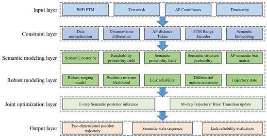
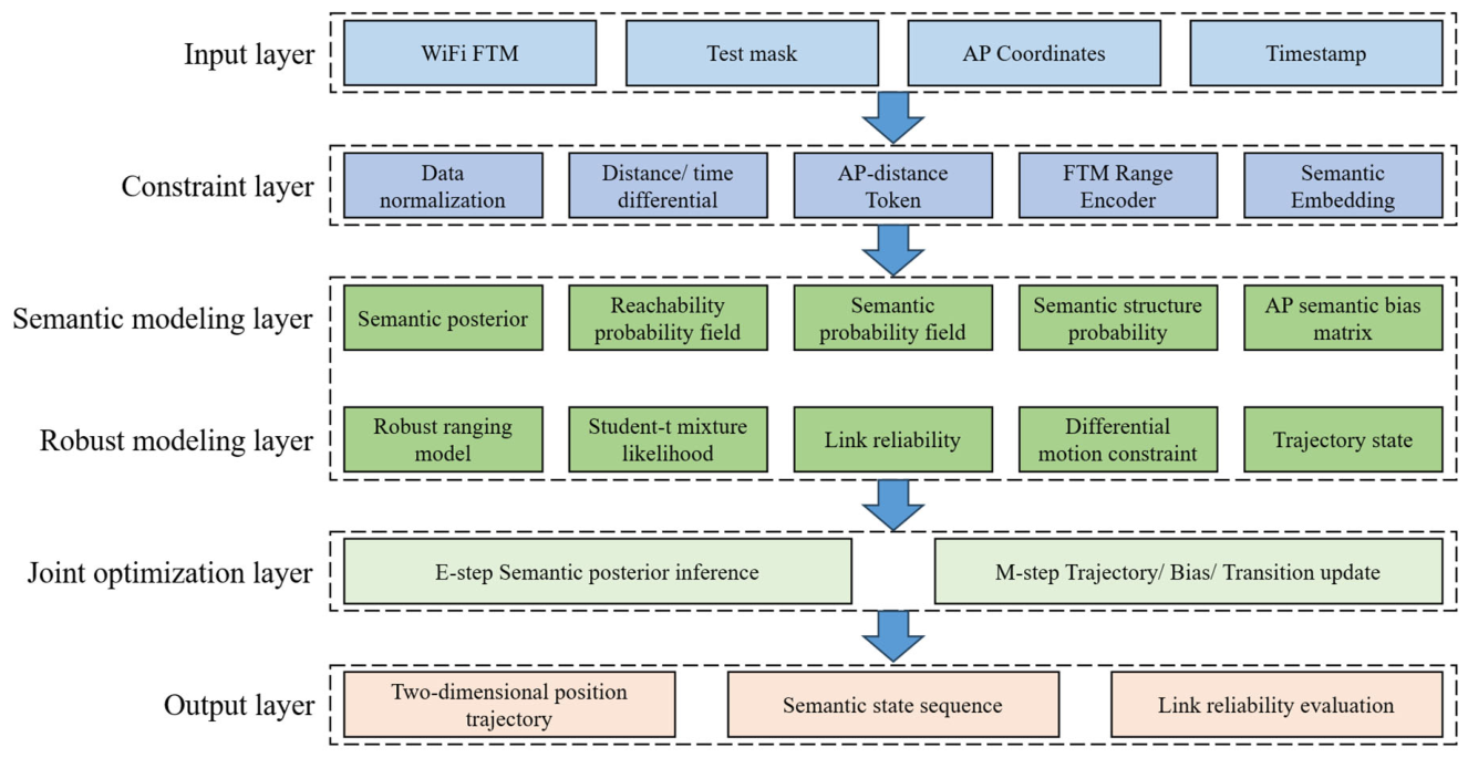
An indoor positioning algorithm based on WiFi FTM multi-objective semantic structure inference is proposed, as shown in Figure 1. This method takes the raw inputs of FTM ranging values, measurability mask, timestamps, and known AP coordinates. It first normalizes the range measurements for each AP. Then, it constructs AP distance vectors, inter-AP distance differences, and temporal differencing to simultaneously characterize the absolute geometric relationship between the terminal and the APs, the relative distance structure, and link visibility. Utilizing the FTM Range Transformer, wireless semantic embeddings are extracted through masked AP distance modeling and time proximity contrastive learning. Clustering or classification yields implicit semantic states reflecting different ranging patterns. A preliminary trajectory is obtained by combining this with robust trilateration. A spatial semantic field driven by the FTM sequence is constructed using state posteriors. A semantic topological graph is established via a state transition matrix. To address indoor NLOS and multipath errors, AP-state-correlated non-negative ranging biases, Student-t mixture likelihood, and mechanisms based on residual change, missing rate, and link reliability gating are introduced. FTM differential constraints and velocity continuity priors are utilized to suppress trajectory jumps. Robust ranging, semantic observations, the spatial semantic field, topological transitions, and differential motion are unified into a joint objective function. The process involves updating the semantic state posterior and link reliability via forward–backward inference. After fixing the state posterior, the position trajectory, velocity, ranging biases, transition matrix, and semantic field are jointly optimized in an alternating manner until the positional variation converges. The final outputs include the positioning trajectory, the sequence of semantic states, and the reliability assessment for each FTM link.

Figure 1. System structure diagram of indoor localization based on semantic structure inference.

3.2. Variable Inputs

Let the two-dimensional localization area be $\mathcal{D}\subset R^2$, and the system deploys $M$ WiFi APs with known coordinates.

$$\begin{array}{c}\mathcal{A}=\left\{{\mathit{a}}_i\in R^2\mid i=1,\dots ,M\right\}\end{array}$$

(1)

At time $t$, a measurable mask is introduced to indicate whether the $\mathrm{i}$-th AP obtains an effective FTM ranging value at that moment.

$$m_{i,t}=\left\{\begin{array}{cc}1,& \mathrm{if} \mathrm{the} i\text{-}\mathrm{th} \mathrm{AP} \mathrm{has} \mathrm{an} \mathrm{effective} \mathrm{ranging} \mathrm{measurement} \mathrm{at} \mathrm{time} t,\\ 0,& \mathrm{otherwise}\end{array}\right.$$

(2)

where $i$ denotes the $\mathrm{i}$-th AP and $t$ denotes the time instant $t$.

The complete data collection set at time $t$ is denoted by ${\mathcal{O}}_t$. ${\mathcal{O}}_t$ combines the ranging value ${\tilde{d}}_{i,t}$ and the measurable mask $m_{i,t}\in \left\{\mathrm{0,1}\right\}$ obtained from the $i$-th AP, as shown in Equation (3).

$$\begin{array}{c}{\mathcal{O}}_t={\left\{\left({\tilde{d}}_{i,t},m_{i,t}\right)\right\}}_{i=1}^M\end{array}$$

(3)

where ${\tilde{d}}_{i,t}$ represents the distance between the terminal and the $i$-th AP at time $t$. It is calculated as ${\tilde{d}}_{i,t}=c\left(t_4-t_1-t_3-t_2\right)/2$, $t_1$ is the time the terminal sends the FTM request, $t_2$ is the time the AP receives the request, $t_3$ is the time the AP sends the response, and $t_4$ is the time the terminal receives the response. $c$ is the speed of light.

The terminal state is written as ${\mathit{x}}_t={\left[{\mathit{p}}_t^{\top },{\mathit{v}}_t^{\top }\right]}^{\top }$, where ${\mathit{p}}_t=\left[\begin{array}{c}{x}_t\\ y_t\end{array}\right]$ is the position coordinate at time $t$, and $v_t\in R^2$ is a velocity variable introduced by internal trajectory constraints, representing the motion state at time $t$. $z_t\in \left\{1,\dots ,k\right\}$ denotes the room category where the terminal is located at time $t$.

3.3. Proposed Method Details

3.3.1. FTM Input

The motivation for this input design is that a single raw FTM distance vector loses two important pieces of information: the relative distance ordering among APs and the change in link visibility over time. The pairwise distance differentials and temporal differences are therefore added to make the encoder sensitive to AP co-occurrence and to short-term ranging changes.

The effectively collected ranging values from the APs are normalized.

$$\begin{array}{c}\begin{array}{c}{\overline{d}}_{i,t}=m_{i,t}{\displaystyle \frac{{\tilde{d}}_{i,t}-{\mu }_i^d}{{\sigma }_i^d}}+\left(1-m_{i,t}\right)c_{miss}\end{array}\end{array}$$

(4)

where ${\mu }_i^d$ is the mean distance for the $i$-th AP, and ${\sigma }_i^d$ is the standard deviation of the distance for the $i$-th AP. $c_{miss}$ is a constant value set for missing measurements. The normalized distance and mask are concatenated to form ${\mathit{y}}_t$, which retains the distance values while also indicating whether the measured distance is reliable.

$$\begin{array}{c}{\mathit{y}}_t={\left[{\overline{d}}_{1,t},\dots ,{\overline{d}}_{M,t},m_{1,t},\dots ,m_{M,t}\right]}^{\mathrm{\top }}\end{array}$$

(5)

Time $t$ represents which AP is closest to the terminal relative to two APs. As shown in Equation (6), the distance differential at time $t$ is defined.

$$\begin{array}{c}\Delta d_{ij,t}=m_{i,t}{m}_{j,t}\left({\tilde{d}}_{i,t}-{\tilde{d}}_{j,t}\right),\hspace{1em}i<j\end{array}$$

(6)

The change in distance from the same AP between two adjacent moments, $t-1$ and $t$, is shown in Equation (7).

$$\begin{array}{c}\mathsf{\nabla }{d}_{i,t}=m_{i,t}{m}_{i,t-1}\left({\overline{d}}_{i,t}-{\overline{d}}_{i,t-1}\right)\end{array}$$

(7)

The final input is represented as ${\mathit{s}}_t^{ftm}$.

$$\begin{array}{c}{\mathit{s}}_t^{ftm}={\left[{\mathit{y}}_t^{\mathrm{\top }},{\left\{\Delta d_{ij,t}\right\}}_{i<j},{\left\{\mathsf{\nabla }{d}_{i,t}\right\}}_{i=1}^M\right]}^{\mathrm{\top }}\end{array}$$

(8)

3.3.2. FTM Range Transformer

A transformer is chosen rather than a fixed feature extractor because FTM measurements form a set of mutually correlated AP tokens whose informativeness depends on the mask. Masked AP-range modeling is used because it forces the encoder to reconstruct a masked AP from the other APs, thereby learning the joint AP distance geometry instead of memorizing individual APs; temporal-proximity contrastive learning further enforces that temporally adjacent observations share similar embeddings. Unlike BERT-style methods that mask scan positions for pseudo-labeling, our masking acts on the AP dimension and the resulting embedding is directly used in the continuous ranging-bias model.

For the AP distance vector of the $i$-th AP at time $t$, see Equation (9).

$$\begin{array}{c}{\tau }_{i,t}=\left({\mathit{a}}_i\cup Q_d\left({\overline{d}}_{i,t}\right)\cup m_{i,t}\right)\end{array}$$

(9)

where ${\mathit{a}}_i$ is the position of the $i$-th AP. $Q_d\left(\cdot \right)$ maps the continuous FTM distance ${\tilde{d}}_{i,t}$ to a discrete interval. The input ${\tau }_{i,t}$ is fed into the transformer encoder $f_{\varphi }$ to obtain the semantic embedding ${\mathit{h}}_t$. ${\mathit{h}}_t$ simultaneously carries three types of information: the relative distance structure between the AP and terminal, the co-occurrence relationship among different APs, and the change in ranging patterns within a short time window.

$$\begin{array}{c}{\mathit{h}}_t=f_{\varphi }\left({\tau }_{1,t},{\tau }_{2,t},\dots ,{\tau }_{M,t}\right)\end{array}$$

(10)

The total training loss of the encoder combines two parts: the classification negative log-likelihood and the time proximity contrastive loss. The first part is the classification negative log-likelihood, where a portion of the information within the set of APs is masked. Based on the unmasked AP information, it predicts the distance interval for the missing one, as shown in Equation (11).

$$\begin{array}{c}{\mathcal{L}}_{MARM}=-{\displaystyle \sum _{t=1}^T}{\displaystyle \sum _{i\in {\mathcal{M}}_t}}{\log p}_{\varphi }\left(Q_d\left({\overline{d}}_{i,t}\right)\mid {\tau }_{j,t}\right)\end{array}$$

(11)

where $j\notin {\mathcal{M}}_t$, ${\mathcal{M}}_t$ is the set of randomly masked APs at time $t$. $p_{\varphi }\left(Q_d\left({\tilde{d}}_{i,t}\right)\mid {\tau }_{j,t}\right)$ represents the model’s prediction probability for the masked AP information after observing the unmasked AP information. $\varphi$ denotes the model parameters. The goal of Equation (11) is to learn the distance relationships between multiple APs and their measurable states rather than to remember the independent information of a single AP.

The second part is the time proximity contrastive loss, as shown in Equation (12). This adopts an InfoNCE-style contrastive learning objective, using observations within the same short time window as positive samples and observations with significantly different distance patterns as negative samples.

$$\begin{array}{c}{\mathcal{L}}_{con}=-{\displaystyle \sum _t}\log {\displaystyle \frac{\exp \left(sim\left({\mathit{h}}_t,{\mathit{h}}_t^{+}\right)/{\tau }_c\right)}{\exp \left(sim\left({\mathit{h}}_t,{\mathit{h}}_t^{+}\right)/{\tau }_c\right)+\sum _{n\in {\mathcal{N}}_t}\exp \left(sim\left({\mathit{h}}_t,{\mathit{h}}_n^{-}\right)/{\tau }_c\right)}}\end{array}$$

(12)

where ${\mathit{h}}_t^{+}$ is the positive sample semantic embedding ${\mathit{h}}_t$ at time $t$, and ${\mathit{h}}_n^{-}$ is a negative sample different from the current sample. ${\mathcal{N}}_t$ denotes the set of negative samples corresponding to the $t$-th sample. $\mathrm{sim}\left(\cdot \right)$ is the cosine similarity, and ${\tau }_c$ is a hyperparameter. The goal of Equation (12) is to make the current sample ${\mathit{h}}_t$ closer to similar positive samples and farther from dissimilar negative samples.

The total training loss for the encoder is given by Equation (13).

$${\mathcal{L}}_{enc}={\mathcal{L}}_{MARM}+{\lambda }_c{\mathcal{L}}_{con}+{\lambda }_{reg}{‖\varphi ‖}_2^2$$

(13)

where ${\lambda }_c$ is the weight coefficient. ${\lambda }_{reg}$ is the regularization weight. ${‖\varphi ‖}_2^2$ represents the L2 norm squared of the model parameters. ${\lambda }_{reg}{‖\varphi ‖}_2^2$ is used to prevent overfitting. The FTM Range Transformer uses 16 AP tokens per time step, where each token is the sum of three learned embeddings: an AP-index embedding, a distance-bin embedding, and a mask embedding. The encoder has two transformer layers with a model dimension of 64, four attention heads, a feed-forward dimension of 128, GELU activation, and pre-layer normalization (no dropout). The distances are discretized into 20 equal-width bins by min-max normalization over the observed ranges. Missing links use bin index 20, and masked tokens use bin index 21. The sequence-level embedding is obtained by mean-pooling the 16 token representations. For the masked AP-range modeling pretraining, 30% of the measurable APs are masked at random, and the model is trained with the Adam optimizer for 1 epoch with a learning rate of 1 × 10⁻³, a batch size of 32, a weight decay of 1 × 10⁻⁵, and a gradient clip norm of 1.0. The semantic classification head is then fine-tuned for 8 epochs with a learning rate of 2 × 10⁻³ and a batch size of 64 using the cross-entropy loss.

Based on the FTM observations at time $t$, the model calculates the probability that the terminal belongs to each hidden state. It then obtains the FTM semantic observation distribution ${\mathit{\pi }}_t^{ftm}$ and its current room category through a semantic classification head.

$${\mathit{\pi }}_t^{ftm}=softmax\left({\mathit{W}}_z{\mathit{h}}_t+{\mathit{b}}_z\right),\hspace{1em}\hspace{1em}{\pi }_{t,k}^{ftm}=p\left(z_t=k\mid {\mathcal{O}}_t\right)$$

(14)

where $\mathit{W}$ is the weight matrix, and $\mathit{b}$ is the bias vector. There is an FTM state probability distribution and a maximum a posteriori state index obtained from current observations.

$${\displaystyle \sum _{k=1}^K}{\pi }_{t,k}^{ftm}=1,\hspace{1em}\hspace{1em}{z}_t={argmax}_{k\in \left\{1,\dots ,K\right\}}{\pi }_{t,k}^{ftm}$$

(15)

To relate the unsupervised state index k to the physical regions without using any region label during localization, the semantic interpretability is assessed offline. Let $c_t^{\ast }\in 1,\dots ,N_c$ be the ground-truth region label at test time t, and let ${\hat{z}}_t=\arg \underset{k}{\max }{\gamma }_{t,k}$ be the smoothed hard state decision, where ${\gamma }_{t,k}$ is the posterior given by the forward–backward algorithm. Note that Equation (14) gives the instantaneous observation likelihood ${\pi }_{t,k}^{ftm}=p\left(z_t=k\mid {\mathcal{O}}_t\right)$, which enters the forward–backward recursion as one factor of the emission probability; hence the mapping uses the temporally smoothed ${\gamma }_{t,k}$ rather than ${\pi }_{t,k}^{ftm}$.

In the final implementation, the state inference is unsupervised: the states are obtained by clustering the self-supervised FTM embeddings, and the softmax head in Equation (14) is parameterized to match the cluster assignments rather than being trained on ground-truth region labels. Since the state indices carry no prior semantic meaning, they are aligned to region indices with an assignment $\sigma :\{1,\dots ,K\}\to \{1,\dots ,N_c\}$, which is a permutation when $K=N_c$ and a partial matching otherwise. The optimal assignment is obtained by maximizing the agreement on the evaluation set:

$${\sigma }^{\ast }=\arg \underset{\sigma }{\max }{\displaystyle \sum _{t=1}^T}1\left\{\sigma \left({\hat{z}}_t\right)=c_t^{\ast }\right\}$$

(16)

which is solved by the Hungarian algorithm from the state-region confusion matrix. This mapping is used only for the offline semantic-consistency evaluation and does not enter the online positioning. The corresponding semantic accuracy is defined as follows.

$${\mathrm{A}\mathrm{c}\mathrm{c}}_{sem}={\displaystyle \frac{1}{T}}{\displaystyle \sum _{t=1}^T}1\left\{{\sigma }^{\ast }\left({\hat{z}}_t\right)=c_t^{\ast }\right\}$$

(17)

which is the optimal one-to-one matching accuracy between the inferred states and the ground-truth regions.

3.3.3. Spatial Semantic Field Generated by FTM

The field is introduced because the robust multilateration initialization is noisy and cannot fully reflect the region structure. By converting the state posterior into a soft spatial field, position hypotheses that are inconsistent with the learned semantic region are penalized smoothly rather than rejected by hard boundaries. This differs from existing semantic localization, which typically enforces hard room or traversable-area constraints.

Obtaining initial positions using robust multilateral positioning.

$$\begin{array}{c}\begin{array}{c}{\mathit{p}}_t^0={argmin}_{\mathit{p}\in \mathcal{D}}{\displaystyle \sum _{i=1}^M}{m}_{i,t}{\rho }_{\delta }\left({\tilde{d}}_{i,t}-{‖\mathit{p}-{\mathit{a}}_i‖}_2\right)\end{array}\end{array}$$

(18)

where ${\rho }_{\delta }$ is the Huber loss. $M$ is the total number of APs. $\mathit{p}$ is a candidate position. This constructs the weighted Kernel Density Estimation ${\mathsf{\Gamma }}_F\left(\mathit{p}\right)$.

$$\begin{array}{c}{\mathsf{\Gamma }}_F\left(\mathit{p}\right)={\displaystyle \frac{1}{C_{\mathsf{\Gamma }}}}{\displaystyle \sum _{t=1}^T}{\omega }_t^{geo}\exp \left(-{\displaystyle \frac{{‖\mathit{p}-{\mathit{p}}_t^{\left(0\right)}‖}_2^2}{2{\sigma }_{\mathsf{\Gamma }}^2}}\right)\end{array}$$

(19)

${\mathsf{\Gamma }}_F\left(\mathit{p}\right)$ represents the spatial region supported by the initial FTM trajectory. ${\sigma }_{\mathsf{\Gamma }}^2$ is the squared bandwidth of the Gaussian kernel for the FTM reachable field, used to control the influence range of the initial position estimate ${\mathit{p}}_t^{\left(0\right)}$ on the surrounding space. This parameter is not obtained directly from a single FTM observation but is set according to the error scale of the initial robust multilateration positioning system. A smaller ${\sigma }_{\mathsf{\Gamma }}$ results in a sharper spatial constraint, while a larger ${\sigma }_{\mathsf{\Gamma }}$ produces a smoother but weaker reachable field.

The semantic posterior probability that the time $t$ belongs to room category $z_t$, given all observations, is denoted by ${\gamma }_{t,k}=p\left(z_t=k\mid {\mathcal{O}}_{1:T}\right)$. The probability of the position state belonging to trajectory $k$ is a soft spatial constraint jointly estimated from the FTM trajectory and the hidden state posterior, as shown in Equation (20).

$${\mathsf{\Psi }}_k\left(\mathit{p}\right)={\displaystyle \frac{{\displaystyle {\sum }_{t=1}^T}{\gamma }_{t,k}\exp \left(-\frac{{‖\mathit{p}-{\mathit{p}}_t‖}_2^2}{2{\sigma }_{\mathsf{\Psi }}^2}\right)}{{\displaystyle {\sum }_{l=1}^K}{\displaystyle {\sum }_{t=1}^T}{\gamma }_{t,l}\exp \left(-\frac{{‖\mathit{p}-{\mathit{p}}_t‖}_2^2}{2{\sigma }_{\mathsf{\Psi }}^2}\right)+ϵ}}$$

(20)

where $l\in z_t$ and $k\in z_t$. ${\sigma }_{\mathsf{\Psi }}^2$ is the squared bandwidth of the Gaussian kernel for the semantic probability field, used to control the semantic diffusion range of trajectory points across the surrounding space. This parameter is not calculated directly from a single observation. It is set based on spatial smoothing requirements, initial trajectory scale, or validation set performance. A smaller ${\sigma }_{\mathsf{\Psi }}$ makes the semantic field more localized, while a larger ${\sigma }_{\mathsf{\Psi }}$ results in a smoother semantic field. $ϵ$ is a constant to prevent division by zero.

3.3.4. Semantic Structure Probability

The transition matrix is added because semantic states have strong temporal adjacency, e.g., a corridor state is typically adjacent to specific rooms. A learned HMM transition suppresses physically implausible state jumps and smooths the state sequence, which is a softer and data-driven alternative to hand-crafted topological constraints.

The soft posterior statistics from adjacent moments, $N_{kl}$, is utilized to estimate the relationship between neighboring room categories in $z_t$.

$$N_{kl}={\displaystyle \sum _{t=2}^T}{\gamma }_{t-1,k}{\gamma }_{t,l}$$

(21)

To alleviate the zero probability issue caused by short sequences or sparse states, a smoothing prior is introduced based on the similarity of the semantic embedding centers: ${\mathsf{\Omega }}_{kl}$ represents the “similarity between state $k$ and state $l$″ for room categories.

$$\begin{array}{c}\begin{array}{c}{\mathsf{\Omega }}_{kl}=\exp \left(-{\displaystyle \frac{{‖{\mathit{\mu }}_k^h-{\mathit{\mu }}_l^h‖}_2^2}{2{\sigma }_h^2}}\right)\end{array}\end{array}$$

(22)

where ${\mathit{\mu }}_k^h={\displaystyle \frac{\sum _t{\gamma }_{t,k}{\mathit{h}}_t}{\sum _t{\gamma }_{t,k}+ϵ}}$, and ${\sigma }_h$ is the scale parameter for semantic center similarity, which controls how quickly the state embedding distance decays. The $2{\sigma }_h^2$ in the denominator adopts the standard form of a Gaussian kernel, used to smoothly map the Euclidean distance into a similarity within the interval $\left(\mathrm{0,1}\right]$.

Based on the Hidden Markov Model (HMM) transition probability estimation, $A_{kl}$ is obtained as the “similarity between state $k$ and state $l$” for room categories.

$$\begin{array}{c}\begin{array}{c}{A}_{kl}=p\left(z_t=l,z_{t-1}=k\mid z_t\right)={\displaystyle \frac{N_{kl}+{\alpha }_A{\mathsf{\Omega }}_{kl}}{{\displaystyle {\sum }_{j=1}^K}\left(N_{kj}+{\alpha }_A{\mathsf{\Omega }}_{kj}\right)}}\end{array}\end{array}$$

(23)

where ${\alpha }_A$ is the transfer smoothing strength hyperparameter.

3.3.5. Semantic Ranging Model and Link Reliability

A constant LOS model is insufficient because FTM errors are correlated with the AP, the semantic region, and the relative direction. The bias is therefore modeled as a low-rank, direction-dependent, non-negative term, and a Student-t mixture likelihood equipped with reliability gating is adopted to suppress the influence of outliers. Unlike existing per-AP constant or binary LOS/NLOS models, our bias varies continuously with position within a semantic region and is jointly estimated with the trajectory.

Under ideal line-of-sight (LOS) conditions, the measured distance ${\tilde{d}}_{i,t}$ can be written as Equation (24).

$$\begin{array}{c}\begin{array}{c}{\tilde{d}}_{i,t}={‖{\mathit{p}}_t-{\mathit{a}}_i‖}_2\end{array}\end{array}$$

(24)

After considering indoor NLOS and multipath propagation, we derive the non-negative AP-state-correlated bias.

$$\begin{array}{c}{\tilde{d}}_{i,t}={‖{\mathit{p}}_t-{\mathit{a}}_i‖}_2+b_{i,z_t}\end{array}$$

(25)

where $b_{i,k}$ (with $k=z_t$) is a non-negative ranging bias associated with AP $i$ and semantic state $k$. For a fixed AP, the bias is constant within a semantic region; it varies across APs and states but does not depend on the terminal’s instantaneous position or direction. LOS, NLOS, and outliers are modeled through a Student-t mixture likelihood.

$$\begin{array}{c}p\left({\tilde{d}}_{i,t}\right)=\sum {\alpha }_{c}T\left(r_{i,t};{\mu }_c,{\sigma }_{i,k,c}^2,{\nu }_c\right)=\sum {\alpha }_c{\displaystyle \frac{\mathsf{\Gamma }\left(\frac{{\nu }_c+1}{2}\right)}{\mathsf{\Gamma }\left(\frac{{\nu }_c}{2}\right)\sqrt{{\nu }_c\pi }\hspace{0.17em}{\sigma }_{i,k,c}}}{\left[1+{\displaystyle \frac{{\left(r_{i,t}-{\mu }_c,\right)}^2}{{\nu }_c{\sigma }_{i,k,c}^2}}\right]}^{-{\displaystyle \frac{{\nu }_c+1}{2}}}\end{array}$$

(26)

where $\sum {\alpha }_c=1$. ${\nu }_c$ is the degrees of freedom parameter, used to control the tail thickness of the Student-t distribution. A larger degree of freedom means the distribution is closer to Gaussian. A smaller degree of freedom results in a thicker tail, making it more robust to anomalous range measurements. ${\mu }_c$ is the location parameter of the c-th Student-t component, i.e., the expected residual offset under component c. The three components use $\left({\mu }_1,{\mu }_2,{\mu }_3\right)=\left(0,0.5,1.5\right)$ m, which correspond to the LOS, NLOS, and outlier regimes, respectively. ${\nu }_c$ can be treated as a hyperparameter or estimated using a validation set. ${\sigma }_{i,k,c}^2$ is the squared Student-t scale parameter correlated with the AP-state component. It is used to describe the discreteness of the residual for this class of ranges. This parameter can be obtained by weighted estimation of residuals bias-corrected from the training data. The residual after range bias correction is $r_{i,t}$.

$$\begin{array}{c}{r}_{i,t}={\tilde{d}}_{i,t}-{‖{\mathit{p}}_t-{\mathit{a}}_i‖}_2-b_{i,z_t}\end{array}$$

(27)

At time $t$, the link reliability of AP $i$ is $q_{i,t}$.

$$\begin{array}{c}{q}_{i,t}=sigmoid\left({\beta }_0-{\beta }_1\left|r_{i,t}\right|-{\beta }_2\left|r_{i,t}-r_{i,t-1}\right|-{\beta }_3{\upsilon }_{i,t}^{miss}\right)\end{array}$$

(28)

where the coefficients ${\beta }_0$, ${\beta }_1$, ${\beta }_2$, and ${\beta }_3$ are non-negative hyperparameters of the reliability gating model. ${\beta }_0$ controls the base reliability. ${\beta }_1$, ${\beta }_2$, and ${\beta }_3$ respectively control the penalty strength of the current residual, residual change, and local missing rate on link reliability. When a link has a large correction residual, rapid changes, frequent local missing measurements, or an unstable impact on the geometric solution, its localization weight is correspondingly reduced.

The local missing rate at time $t$ is ${\upsilon }_{i,t}^{miss}$.

$$\begin{array}{c}{\upsilon }_{i,t}^{miss}=1-{\displaystyle \frac{1}{2L+1}}{\displaystyle \sum _{\mathcal{l}=-L}^L}{m}_{i,t+\mathcal{l}}\end{array}$$

(29)

where $L$ is the window half-width and $l$ is the window offset. This represents the missing rate of AP $i$ over the $2L+1$ time steps centered at time $t$.

3.3.6. FTM Differential Motion Constraint

This constraint is added to obtain temporal continuity directly from consecutive FTM ranges. It suppresses abrupt trajectory jumps without requiring an inertial sensor, which is an advantage over PDR/IMU-based methods that need additional hardware.

The local continuity of the trajectory is constrained by utilizing the change in adjacent FTM range measurements. $\Delta {\mathit{p}}_t$ is the displacement vector of the terminal from time $t-1$ to time $t$, where $\Delta {\mathit{p}}_t={\mathit{p}}_t-{\mathit{p}}_{t-1}$.

$$\begin{array}{c}{‖{\mathit{p}}_t-{\mathit{a}}_i‖}_2-{‖{\mathit{p}}_{t-1}-{\mathit{a}}_i‖}_2\approx {\mathit{u}}_{i,t-1}^{\mathrm{\top }}\Delta {\mathit{p}}_t\end{array}$$

(30)

where $\begin{array}{c}\begin{array}{c}{\mathit{u}}_{i,t-1}={\displaystyle \frac{{\mathit{p}}_{t-1}-{\mathit{a}}_i}{{‖{\mathit{p}}_{t-1}-{\mathit{a}}_i‖}_2+ϵ}}\end{array}\end{array}$ is the unit direction vector pointing from AP $i$ to the terminal’s position at the previous time step $t-1$.

Derive its range-differencing residual based on Equation (27).

$$\begin{array}{c}{r}_{i,t}^{\Delta }=\left({\tilde{d}}_{i,t}-{\tilde{d}}_{i,t-1}\right)-{\mathit{u}}_{i,t-1}^{\mathrm{\top }}\left({\mathit{p}}_t-{\mathit{p}}_{t-1}\right)-\left(b_{i,z_t}-b_{i,z_{t-1}}\right)\end{array}$$

(31)

Obtain the corresponding differential energy.

$$\begin{array}{c}{E}_{\Delta }\left(t\right)={\displaystyle \sum _{i=1}^M}{m}_{i,t}{m}_{i,t-1}{q}_{i,t}{q}_{i,t-1}{\rho }_{\delta }\left({\displaystyle \frac{r_{i,t}^{\Delta }}{{\sigma }_{\Delta ,i}}}\right)\end{array}$$

(32)

where ${\rho }_{\delta }\left(\cdot \right)$ is the Huber loss function, and ${\sigma }_{\Delta ,i}$ is the scale parameter of the differential residual for AP $i$.

Motion continuity constraint from time $t-1$ to time $t$.

$$\begin{array}{c}{E}_{kin}\left(t\right)={‖{\mathit{p}}_t-{\mathit{p}}_{t-1}-{\mathit{v}}_{t-1}\Delta t‖}_{{\mathsf{\Sigma }}_p^{-1}}^2+{‖{\mathit{v}}_t-{\mathit{v}}_{t-1}‖}_{{\mathsf{\Sigma }}_v^{-1}}^2\end{array}$$

(33)

where ${\mathsf{\Sigma }}_p^{-1}$ and ${\mathsf{\Sigma }}_v^{-1}$ are weighted norms in the Mahalanobis distance form. ${\mathit{v}}_t={\displaystyle \frac{{\mathit{p}}_t-{\mathit{p}}_{t-1}}{\Delta t}}$ is the displacement velocity.

3.4. Joint Optimization Objective and State Update

A single joint objective is used because the components are mutually dependent: the semantic state depends on the position, the bias depends on the state, and the semantic field depends on both. Alternating between the forward–backward state update and the geometric optimization keeps the problem tractable while still estimating the semantic and geometric states jointly, unlike the more common classify-then-regress pipeline.

3.4.1. Joint Objective Function

The reliability-weighted robust ranging energy is defined as $E_{range}\left(t\right)$.

$$\begin{array}{c}{E}_{range}\left(t\right)={\displaystyle \sum _{i=1}^M}{m}_{i,t}{w}_{i,t}{\rho }_{\delta }\left({\displaystyle \frac{{\tilde{d}}_{i,t}-{‖{\mathit{p}}_t-{\mathit{a}}_i‖}_2-b_{i,z_t}}{{\sigma }_{i,z_t}}}\right)\end{array}$$

(34)

where $w_{i,t}=q_{i,t}+{\lambda }_N\left(1-q_{i,t}\right)$, and $0<{\lambda }_N<1$. The semantic observation energy, position-semantic consistency energy, and topological transition energy are as follows.

$$\begin{array}{cc}\hfill E_{sem}\left(t\right)& =-\log \left({\pi }_{t,z_t}^{ftm}+ϵ\right)\hfill \\ \hfill E_{field}\left(t\right)& =-\log \left({\mathsf{\Gamma }}_F\left({\mathit{p}}_t\right)+ϵ)-\log \left({\mathsf{\Psi }}_{z_t}\left({\mathit{p}}_t\right)+ϵ),\right)\right)\hfill \\ \hfill E_{topo}\left(t\right)& =-\log \left(A_{z_{t-1},z_t}+ϵ\right)\hfill \end{array}$$

(35)

where $ϵ$ is a small constant. To reduce the degrees of freedom of the AP-state bias matrix in sparse data, a low-rank parameterization is employed.

$$b_{i,k}=softplus\left(u_i^T{c}_k+{\eta }_i+{\zeta }_k\right)=ln\left(1+exp\left(u_i^T{c}_k+{\eta }_i+{\zeta }_k\right)\right)$$

(36)

where $u_i\in R^r$ and $c_k\in R^r$ are learned low-rank AP-specific and state-specific vectors with rank $r=4$, and ${\eta }_i$, ${\zeta }_k$ are AP and state scalar offsets. This parameterization keeps the bias constant within a semantic region for a given AP while reducing the number of free parameters in sparse data. The low-rank term $u_i^T{c}_k$ captures AP-state interactions, while ${\eta }_i+{\zeta }_k$ provides AP- and state-level offsets. The regularization term is as follows.

$$\begin{array}{c}{E}_{bias}={\lambda }_u{\displaystyle \sum _i}{‖{\mathit{u}}_i‖}_2^2+{\lambda }_c{\displaystyle \sum _k}{‖{\mathit{c}}_k‖}_2^2+{\lambda }_{\eta }{\displaystyle \sum _i}{\eta }_i^2+{\lambda }_{\zeta }{\displaystyle \sum _k}{\zeta }_k^2\end{array}$$

(37)

The final objective function is as follows.

$$\begin{array}{cc}\mathcal{J}=& {\lambda }_r{\displaystyle \sum _{t=1}^T}{E}_{range}\left(t\right)+{\lambda }_s{\displaystyle \sum _{t=1}^T}{E}_{sem}\left(t\right)+{\lambda }_f{\displaystyle \sum _{t=1}^T}{E}_{field}\left(t\right)\\ \hspace{1em}& +{\lambda }_d{\displaystyle \sum _{t=2}^T}{E}_{\Delta }\left(t\right)+{\lambda }_k{\displaystyle \sum _{t=2}^T}{E}_{kin}\left(t\right)+{\lambda }_a{\displaystyle \sum _{t=2}^T}{E}_{topo}\left(t\right)+E_{bias}\end{array}$$

(38)

The weighting coefficients are fixed to $\lambda r=\lambda s=\lambda f=1$, $\lambda d=\lambda k=0.22$, and $\lambda a=1.0$, while the bias regularization weight is 0.05. Each residual term is normalized by its scale parameter, and the smoothing strengths are selected on the validation set. Because the terms are coupled through the latent states, the objective is not jointly minimized. It is solved with an alternating EM-style procedure described in Section 3.4.2.

In this objective function, the ranging term provides local geometric constraints. The semantic term provides observation pattern constraints. The semantic field provides spatial and temporal structure. The differential and motion terms suppress trajectory jumps. The bias regularization term controls model complexity.

3.4.2. Semantic State Update

This paper adopts an alternating update strategy for semantic state and geometric state. Given the current trajectory, biases, and semantic field, the emission probability of state $k$ at time $t$, denoted as ${\phi }_t\left(k\right)$, is defined.

$$\begin{array}{c}{\phi }_t\left(k\right)={\pi }_{t,k}^{ftm}{\mathsf{\Psi }}_k\left({\mathit{p}}_t\right){\displaystyle \prod _{i=1}^M}{\left[p\left({\tilde{d}}_{i,t}\right)\right]}^{m_{i,t}}\end{array}$$

(39)

The forward–backward algorithm for the HMM obtains the posterior probability.

$$\begin{array}{cc}\hfill {\alpha }_t\left(k\right)& ={\phi }_t\left(k\right){\displaystyle \sum _{j=1}^K}{\alpha }_{t-1}\left(j\right)A_{jk},\hfill \\ \hfill {\beta }_t\left(k\right)& ={\displaystyle \sum _{j=1}^K}{A}_{kj}{\phi }_{t+1}\left(j\right){\beta }_{t+1}\left(j\right),\hfill \\ \hfill {\gamma }_{t,k}& ={\displaystyle \frac{{\alpha }_t\left(k\right){\beta }_t\left(k\right)}{{\displaystyle {\sum }_{l=1}^K}{\alpha }_t\left(l\right){\beta }_t\left(l\right)+ϵ}}\hfill \end{array}$$

(40)

${\alpha }_t\left(k\right)$ is the forward probability, representing the likelihood that the room type at time $t$ is $k$. ${\beta }_t\left(k\right)$ is the backward probability, representing the likelihood that the observations from the next time step onwards can be explained. ${\gamma }_{t,k}$ is the final state probability, which is the probability of being in room type $k$ at time $t$ after observing the entire sequence.

$q_{i,t}$ is updated based on the residual and missing rate. After fixing ${\gamma }_{t,k}$, biases are fitted using weighted residuals, room category is updated based on new soft-state counts, and ${\mathsf{\Gamma }}_F$ and ${\mathsf{\Psi }}_k$ are recalculated. In the M-step, the positions are refined time step by time step with robust Gauss–Newton using the Huber loss ($\delta =1.6$, $damping 1\times {10}^{-3}$, at most 10 inner iterations per time step), followed by temporal smoothing with weight 0.22. The low-rank semantic bias is fitted by gradient descent for 250 steps with learning rate 0.05, rank 4, and ridge penalty 0.05. The link reliability is updated by a sigmoid score $2.2-0.65\left|r\right|-0.22\mathsf{\Delta }r-1.4·\left(local missing rate\right)$, clipped to [0.08, 0.98].

The process stops when the average position change between adjacent rounds is less than a threshold or when the maximum number of iterations is reached. The algorithm flow is shown in Algorithm 1.

Algorithm 1. Semantic Structure Inference Localization Algorithm.

Require: FTM sequence ${\mathcal{O}}_{1:T}$, AP coordinates $A$, number of states $K$. Ensure: Position trajectory ${\stackrel{\mathit{ˆ}}{\mathit{p}}}_{1:T}$, State sequence ${\hat{z}}_{1:T}$, Reliability ${\hat{q}}_{i,t}.$

1. Construct normalized distances, inter-AP distance differences, temporal differencing, and AP distance vectors. 2. Pretrain the FTM Range Transformer using MARM and time proximity contrastive loss. 3. Obtain initial position estimate ${\mathbf{p}}_t^{\left(0\right)}$ via robust trilateration. 4. Initialize $\gamma$, $\mathbf{A}$, and low-rank biases based on FTM embeddings and initial positions. 5. Repeat 6. Update ${\gamma }_{t,k}$ using the forward–backward algorithm. 7. Update $q_{i,t}$ based on FTM residuals, missing rates, and geometric contributions. 8. Update biases, trajectory, transition matrix, and semantic probability field. 9. Until average position change is below a threshold or reaches maximum iterations. 10. Output ${\stackrel{\mathit{ˆ}}{\mathit{p}}}_t$, ${\hat{z}}_t={{\mathrm{argmax}}_k\gamma }_{t,k}$, and ${\hat{q}}_{i,t}$.

4. Experiments and Experimental Analysis

4.1. Data Collection

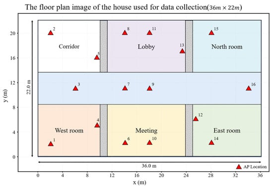
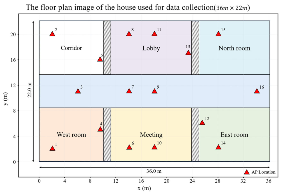
This experiment is conducted in an indoor area of $36 \mathrm{m}\times 22 \mathrm{m}$. The indoor area, shown in Figure 2, contains six types of regions: corridor, west-side room, east-side room, conference area, hall, and north-side room. The house is equipped with 16 access points that support IEEE 802.11 mc (Wi-Fi FTM). The APs were mounted on the ceiling at a height of approximately 2.8 m. To obtain the ground-truth coordinates, a set of reference points was pre-marked on the floor of the experimental area and surveyed with a laser rangefinder (DELI-DL4171, accuracy $\approx \pm 3$ mm) relative to a local Cartesian coordinate system fixed by the room corners. The collected data includes ranging values, masks, timestamps, and AP coordinates. The route sequentially covers the west-side room, corridor, conference room, corridor, east-side room, corridor, hall, corridor, north-side room, and finally returns to the vicinity of the west-side room.

Figure 2. Experimental data collection area.

The mobile terminal was an ESP32-S3 development board running ESP-IDF and configured as the FTM initiator. At each epoch, with a sampling interval of 1 s, the terminal initiated one FTM session with each reachable AP and collected 16 FTM bursts per session. Each range is computed as $d=c·\left(t4-t1-\left(t3-t2\right)\right)/2$, where $t1-t4$ are the request/response timestamps defined in Section 3.2, and the bursts are combined by the mean to produce one range per AP per epoch. Links whose FTM status indicates failure, or whose received signal strength is below −75 dBm, are marked as unavailable in the measurability mask. Before localization, a static calibration at a known distance was used to estimate and remove the common clock-offset bias.

The training session contains 1200 time steps with a total path length of 178.3 m and a mean walking speed of approximately 0.15 m/s. The test session contains 400 time steps with a total path length of 154.1 m and a mean walking speed of approximately 0.4 m/s. Both trajectories cover all six semantic regions, but the coverage is unbalanced: for example, the north room accounts for 7.2% of training samples but only 0.25% of test samples. The two sessions are temporally independent. Their timestamps start from zero independently. But the trajectories overlap spatially, since about 25.5% of the test points lie within 0.5 m of the training trajectory.

4.2. Experimental Analysis

The proposed method is compared with ten baseline algorithms from three categories. The geometric FTM methods are least-squares multilateration (FTM-LS), robust Huber multilateration (FTM-Huber), weighted least-squares multilateration (WLS), and particle swarm optimization (PSO). The fingerprinting and learning-based methods are k-nearest neighbor (KNN), weighted KNN (WKNN), a multilayer perceptron (ANN), random forest (RF), and support vector regression (SVR). The Bayesian filtering baseline is a particle filter.

To ensure a fair comparison, all methods use the same 16 AP coordinates, the same FTM range measurements, the same measurability masks, and the same training/test split. Geometric and PF methods use only the test-time range observations, while fingerprinting and learning-based methods use the training trajectory described in Section 4.1 as the offline radio map. A test step is evaluated only when at least three valid AP measurements are available. Table 1 summarizes the key baseline configurations. Table 2 reports the RMSE, MAE, median error, and 90th-percentile error. For KNN, WKNN, ANN, RF, and SVR, the input feature is the 16-dimensional vector of per-AP normalized FTM distances; missing AP measurements are set to zero.

Table 1. These are various algorithm configurations.

Algorithm	Key Configuration
FTM-LS	grid step 0.75 m, common-offset correction, Gauss–Newton, L2 loss
FTM-Huber	common-offset correction, Huber loss with $\delta =1.5$
WLS	iteratively reweighted by $w=1/{\left(1+\left(r/1.5\right)\right)}^2$
PSO	30 particles, 25 iterations, inertia $\omega =0.5,$$c1=c2=1.5$
KNN	$k=5,$ Euclidean distance, arithmetic mean
WKNN	$k=5,$ inverse-distance weights $1/\left(d+{10}^{-6}\right)$
ANN	MLP 16-32-2, ReLU, $lr=0.001,$ 15 epochs
RandomForest	100 trees, random_state = 7
SVR	RBF kernel, $C=1.0,$$\epsilon =0.1,$$\gamma =scale$
ParticleFilter	1000 particles, ${\sigma }_q=0.3$ m, ${\sigma }_r=1.5$ m

Table 2. Comparison of different algorithms.

Algorithm	RMSE	MAE	Median Error	90th Percentile Error
FTM-LS	2.4895	1.6718	1.0173	3.8339
FTM-Huber	1.5872	1.2835	1.0273	2.3231
WLS	1.6263	1.3023	1.016	2.5667
PSO	1.0899	0.9161	0.7391	1.8336
KNN	2.0272	1.5875	1.2896	3.1032
WKNN	2.019	1.5828	1.3019	3.0418
ANN	1.4139	1.1938	1.0075	2.0902
RandomForest	2.0889	1.4764	0.9245	3.1352
SVR	1.4472	1.0449	0.7217	2.2145
ParticleFilter	3.5324	2.2538	1.3846	4.2844
Proposed	0.6904	0.6559	0.6353	0.9040

Table 2 reports the RMSE, MAE, median error, and 90th-percentile error of the proposed method and the ten baselines. Among the geometric methods, FTM-Huber (RMSE 1.5872 m, MAE 1.2835 m) and WLS (RMSE 1.6263 m, MAE 1.3023 m) clearly outperform FTM-LS (RMSE 2.4895 m, MAE 1.6718 m), confirming that robust weighting is helpful in suppressing the NLOS and outlier errors present in the FTM measurements. PSO further reduces the geometric error and achieves the best result in this group (RMSE 1.0899 m, MAE 0.9161 m, P90 1.8336 m). For the fingerprinting and learning-based methods, KNN and WKNN show similar accuracy, while WKNN obtains slightly better RMSE and P90 (2.0190 m and 3.0418 m versus 2.0272 m and 3.1032 m). The ANN baseline improves the RMSE and MAE to 1.4139 m and 1.1938 m, respectively. RandomForest reaches a low median error of 0.9245 m but has a relatively high RMSE of 2.0889 m and P90 of 3.1352 m, indicating an unstable tail performance. SVR obtains a median error of 0.7217 m and a P90 of 2.2145 m, which are the best among the non-geometric baselines. The particle filter yields the largest error (RMSE 3.5324 m, P90 4.2844 m) because its per-step range observation model does not exploit the semantic structure and temporal constraints. In contrast, the proposed method achieves the minimum value on all four metrics: RMSE 0.6904 m, MAE 0.6559 m, median error 0.6353 m, and P90 0.9040 m. Compared with the best baseline, PSO, it reduces the RMSE by 36.7%, the MAE by 28.4%, and the P90 by 50.7%, demonstrating both higher accuracy and much better robustness to large ranging errors.

Table 3 reports the percentage error reduction in the proposed method relative to each baseline, computed as (baseline error − proposed error)/baseline error × 100%. All values are positive, indicating that the proposed method strictly improves every metric for every compared method. The largest reductions are obtained against ParticleFilter, whose range-only and step-wise observation model benefits most from the semantic structure and temporal constraints: the RMSE, MAE, and median error are reduced by 80.46%, 70.90%, and 54.12%, respectively. The proposed method also reduces the RMSE of FTM-LS by 72.27% and its MAE by 60.77%, confirming that robust semantic inference substantially alleviates the NLOS and outlier errors that dominate pure least-squares multilateration. Among the fingerprinting methods, KNN and WKNN show similar improvements of about 65.9% and 65.8% in RMSE, while RandomForest achieves a 66.95% RMSE reduction but only a 31.28% median reduction, which is consistent with its long error tail in Table 2. Compared with the best geometric baseline, PSO, the proposed method reduces the RMSE, MAE, and median error by 36.65%, 28.40%, and 14.04%, respectively; compared with the best learning-based baseline, SVR, the corresponding reductions are 52.29%, 37.23%, and 11.97%. The median improvements are generally smaller than the RMSE and MAE improvements because several baselines already reach sub-meter median errors. The proposed method still achieves the lowest median error and, more importantly, a substantially smaller RMSE, which indicates stronger robustness against large positioning errors.

Table 3. The percentage reduction in error of the proposed method compared to each of the benchmark methods.

Algorithm	RMSE(%)	MAE(%)	Median Error (%)
FTM-LS	72.26752	60.76684	37.55038
FTM-Huber	56.50202	48.89755	38.15828
WLS	57.54781	49.63526	37.47047
PSO	36.65474	28.40301	14.04411
KNN	65.94317	58.68346	50.73666
WKNN	65.80485	58.56078	51.20209
ANN	51.17052	45.0578	36.94293
RandomForest	66.94911	55.57437	31.28177
SVR	52.29409	37.22844	11.97173
ParticleFilter	80.45521	70.89804	54.11671

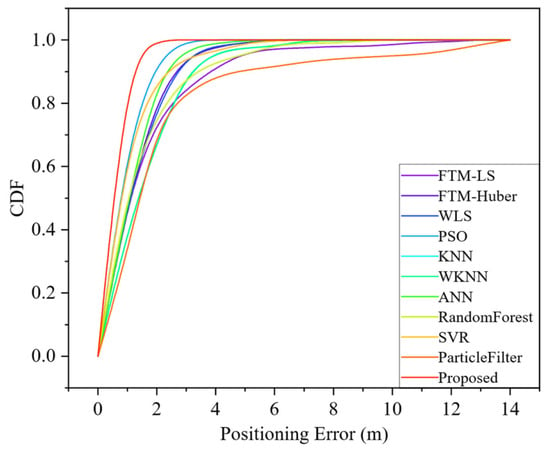
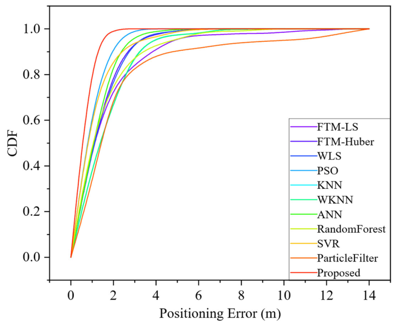
The cumulative distribution function (CDF) curves of the four algorithms are compared, which reflect the overall distribution characteristics and the probability of achieving a given performance level for each algorithm.

Figure 3 presents the cumulative distribution functions of the positioning errors for the proposed method and the ten baselines. The horizontal axis is the positioning error and the vertical axis is the cumulative probability. A curve located farther to the left and rising more steeply indicates that a larger proportion of samples achieve smaller errors. The proposed method is located farthest to the left and rises most steeply, meaning that its error distribution dominates all baselines across nearly the entire error range. Among the baselines, PSO and SVR are the closest competitors, followed by ANN, FTM-Huber, and WLS. RandomForest rises quickly in the small-error region but exhibits a relatively long right tail, which is consistent with its large 90th-percentile error in Table 2. The KNN, WKNN, and ParticleFilter curves are shifted to the right, with ParticleFilter producing the widest error distribution and the heaviest tail. These results are consistent with Table 2: the proposed method achieves the smallest median and 90th-percentile errors, while ParticleFilter shows the largest errors. Therefore, this CDF comparison visually demonstrates that the proposed algorithm can achieve higher cumulative probabilities at a lower cost or smaller metric value across most sample scenarios, exhibiting superior efficiency, robustness, and comprehensive performance.

Figure 3. Comparison of CDF curves for different algorithms.

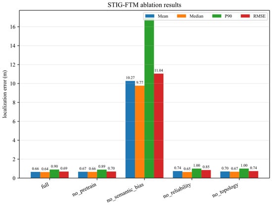
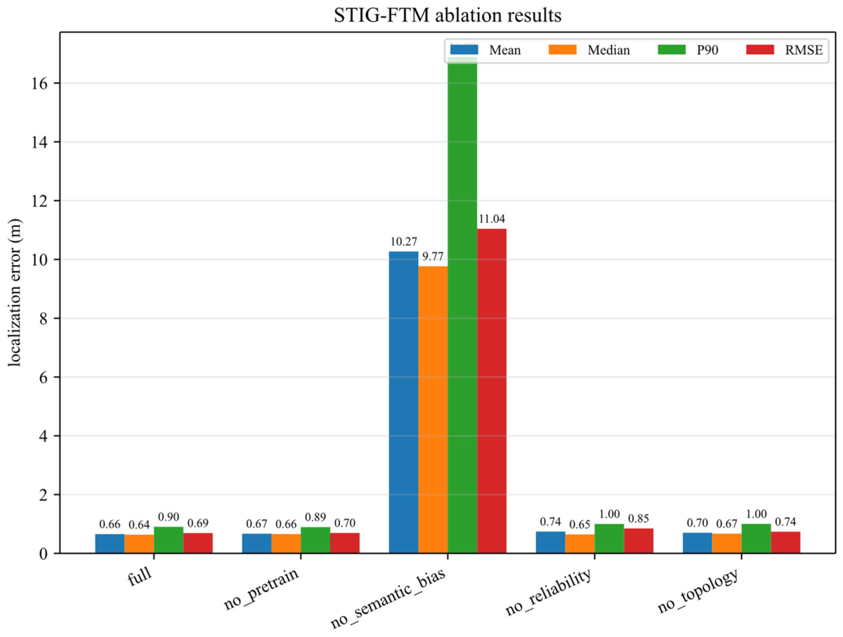
Figure 4 decomposes the contribution of each component using four complementary error metrics. The four metrics characterize different aspects of the error distribution: Mean and Median describe the central tendency, P90 describes the upper tail, and RMSE emphasizes large errors through quadratic weighting. For the complete model, the mean (0.66 m) and the median (0.64 m) are very close, and the RMSE (0.69 m) is only slightly above the mean. This near-overlap indicates a compact, approximately symmetric error distribution with only mild right skew. The P90 of 0.90 m further shows that 90% of samples are confined within about 1 m, which is the practically relevant operating range for indoor positioning.

Figure 4. Ablation study overall results.

“No pretrain” means skipping the self-supervised MARM/contrastive pre-training of the FTM Range Transformer while retaining the subsequent supervised semantic fine-tuning. The fine-tuning uses the ground-truth semantic-region labels of the 1200-step training trajectory (indices 0–5 for the six regions). The test sequence is not used for any encoder parameter learning; it is only processed in a forward pass to produce the semantic embeddings used by the per-test alternating optimization. The pre-training and topology ablations are nearly indistinguishable from those of the complete model. All four metrics change by at most a few centimeters. This observation carries two implications. First, the joint objective already receives strong constraints from the semantic and reliability terms, so the additional information supplied by pre-training and topology is largely redundant in this setting. Second, their contribution is likely indirect: pre-training mainly provides a better initialization for the FTM Range Transformer, and topology mainly smooths state transitions. Such benefits are more likely to appear under sparse data or long-sequence reasoning than in the current test regime.

The reliability ablation reveals a more specific role. Removing reliability barely moves the median (0.64 m to 0.65 m) but clearly raises the P90 (0.90 m to 1.00 m) and the RMSE (0.69 m to 0.85 m). This asymmetric pattern is exactly what the Student-t mixture likelihood and link-quality gating are designed to produce. Reliability modeling does not improve the typical sample; it suppresses the influence of a small number of degraded or inconsistent links. The divergent behavior of the median and the RMSE therefore provides direct evidence that reliability acts on the tail rather than the body of the error distribution.

The semantic-bias ablation dominates all others. Its mean, median, P90, and RMSE are 10.27 m, 9.77 m, 16.89 m, and 11.04 m, roughly fifteen times the complete-model values. Two features are notable. The median also degrades catastrophically, which distinguishes this failure from the reliability case. The problem is therefore not a few outliers but a systematic loss of constraint across essentially all samples. The P90 and RMSE rise even faster than the mean, implying that the residual errors also become heavy-tailed. This is consistent with the interpretation that the semantic bias module establishes the fundamental mapping between observation features and spatial positions. Once this mapping is removed, the remaining terms cannot correct the systematic ranging biases, and the error becomes both larger and more heterogeneous.

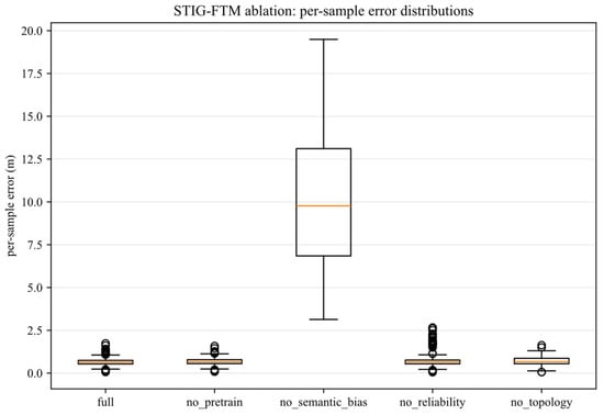
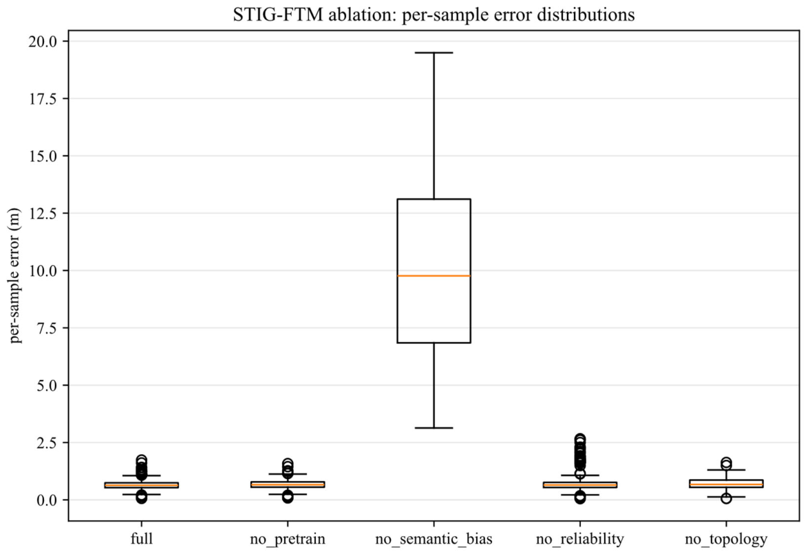
Figure 5 complements Figure 4 by exposing the full distributional shape rather than scalar summaries. The complete model shows a tight box with a short whisker range and only a sparse set of outliers. The concentration of the interquartile range confirms that the good performance is not achieved by averaging over a scattered distribution; rather, the vast majority of samples are genuinely well localized.

Figure 5. Per-sample error distribution.

The pre-training and topology ablations leave the box position, interquartile range, and whiskers almost unchanged. This distributional invariance is stronger evidence than the scalar metrics alone: it shows that these modules do not merely preserve the average, but leave the entire error distribution intact. Their removal does not create new failure modes.

The reliability ablation changes the distribution in a highly asymmetric way. The median and the box body remain nearly fixed, but the upper whisker lengthens and the number of high-error outliers grows. This is the distributional signature of tail inflation without a location shift. It confirms that reliability modeling functions as an outlier-suppression mechanism, and that its benefit concentrates precisely in the samples that the robust likelihood and gating terms are intended to handle.

The semantic-bias ablation produces a qualitatively different distribution. The entire box shifts upward and widens, with the interquartile range expanding by an order of magnitude and the upper whisker reaching approximately 19 m. Unlike the reliability case, this is a location-and-scale shift affecting the majority of samples. Such a transformation indicates a structural failure: the model can no longer distinguish among candidate spatial states, so the errors become diffuse rather than locally concentrated. This observation links the empirical degradation directly to the role of semantic information in constraining the search space.

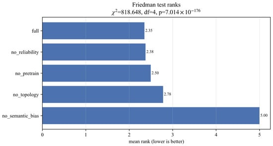
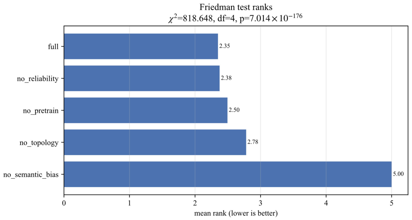
The Friedman test is appropriate here because the per-sample errors are non-Gaussian and heavy-tailed, so a rank-based non-parametric procedure is more robust than an ANOVA-style comparison. In Figure 6, the average ranks order the configurations as complete (2.35), no reliability (2.38), no pretrain (2.50), no topology (2.78), and no semantic bias (5.00). The test statistic ${\chi }^2=818.648$ with four degrees of freedom is extraordinarily large, yielding $p=7.01\times {10}^{-176}$. This is effectively decisive evidence against the null hypothesis of no systematic difference.

Figure 6. Friedman overall significance test.

Two points deserve emphasis. First, the statistical result does not depend on any single metric; it reflects consistent ranking across multiple related comparison units. The significance therefore cannot be dismissed as an artifact of a particular error definition. Second, the rank ordering already reveals where the significance originates. The four top-ranked configurations cluster within a narrow band from 2.35 to 2.78, while the semantic-bias ablation is separated at 5.00. This gap indicates that the overall significance is driven almost entirely by one catastrophic ablation rather than by small differences among the supporting modules.

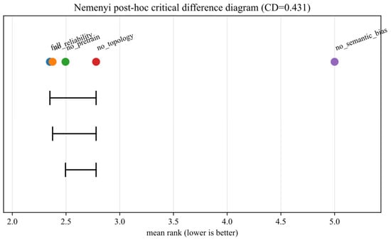
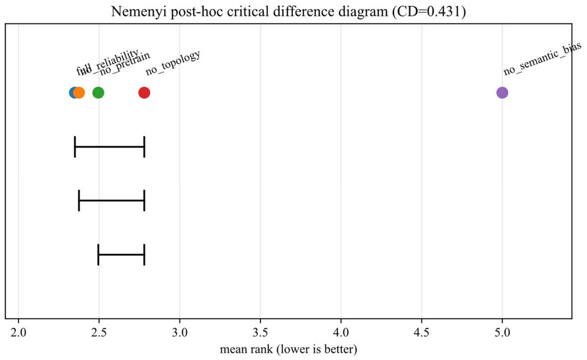
The Nemenyi test sharpens the Friedman result by controlling the family-wise error across all pairwise comparisons. Figure 7 shows Nemenyi post hoc critical difference analysis. With a critical difference of $CD=0.431$, the diagram connects the complete model, no reliability, no pretrain, and no topology into a single statistically indistinguishable group. The semantic-bias ablation stands alone at rank 5.00 and is separated from every other configuration by a margin far exceeding the critical difference.

Figure 7. Nemenyi post hoc critical difference analysis.

This grouping has an important interpretative consequence. Several modules produce measurable metric changes in Figure 4—most visibly the reliability module—yet the Nemenyi test does not separate them from the complete model. This is a distinction between practical and statistical significance. The reliability module yields real improvements in P90 and RMSE, but after multiple-comparison correction the rank differences do not exceed CD. Conversely, the semantic-bias module is the only component whose removal induces a difference that survives this correction. The diagram therefore identifies semantic bias as the only component with unambiguous, replicable, and statistically separable contribution under the current data.

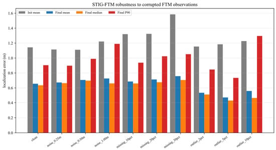
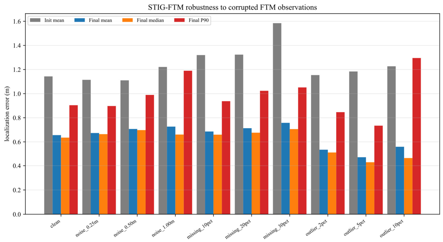
To further validate the robustness of the proposed algorithm under polluted observation conditions, Figure 8 presents the robustness validation in complex pollution scenarios. Figure 8 tests the method against three failure modes that target different parts of the pipeline. Random noise perturbs the ranging measurements themselves, missing observations remove information, and outliers inject gross errors that resemble non-line-of-sight conditions. The four curves—initial mean, final mean, final median, and final P90—separate the difficulty of the input from the quality of the output.

Figure 8. Robustness validation under complex pollution conditions.

The contamination was injected into the test ranges as follows. (i) Random noise: Gaussian noise $N\left(0,\sigma \right)$ with $\sigma \in \{0.25,0.50,1.00\}$ m was added to all observed ranges. (ii) Missing observations: each observed link was independently removed with probability 10%, 20%, or 30% by setting its mask to zero. (iii) Outliers: each observed link was independently selected with probability 2%, 5%, or 10%, and a positive offset sampled uniformly from [2,4] m was added to its range. All perturbations were applied only to the test sequence.

The most consistent finding is the compression between the initial and final errors. Under clean conditions, the initial mean of about 1.10 m is reduced to a final mean of about 0.63 m. A similar gap is maintained under every corruption, which quantifies the correction capability of the optimization stage and shows that the model actively resolves rather than merely reports the input uncertainty.

The missing-data scenario is the most informative for understanding the model’s information structure. The initial mean degrades sharply as the missing ratio grows, reaching about 1.52 m at 30% missing. In contrast, the final mean rises only to about 0.73 m. This resilience implies that the semantic field, the reliability evaluation, and the temporal topology jointly substitute for the lost observations. The model is therefore able to extrapolate from the remaining evidence, which is a direct demonstration of the redundancy designed into the multi-objective formulation.

The outlier scenario isolates the contribution of the heavy-tailed likelihood. For 2%, 5%, and 10% outliers, the final mean stays low (about 0.51 m, 0.45 m, and 0.54 m), showing that the central estimate is not dominated by contaminated links. However, the final P90 rises to about 1.25 m at the 10% outlier level. This divergence between the mean and the 90th percentile is analytically meaningful: the robust likelihood bounds the influence of outliers on the central estimate, but it cannot fully eliminate the residual tail risk when contamination is dense. The result therefore delineates both the strength and the limit of the robustness mechanism. Under outlier injection, the final error slightly decreases as the outlier ratio increases. This is because the injected outliers are positive offsets, which produce large positive residuals. The link-reliability gate suppresses links with large residuals toward its floor, so the robust Gauss–Newton update is increasingly dominated by the remaining clean links. In the clean setting, mildly biased links are not down-weighted and can still perturb the solution. Consequently, a higher outlier ratio leads to a cleaner effective set of observations after reliability gating.

The noise scenario shows a milder but monotonic response, with the final mean rising from about 0.65 m to 0.70 m and the final P90 from about 0.86 m to 1.14 m as noise intensity increases. Unlike outliers, which are sparse and thus well suppressed, noise corrupts every link uniformly. The larger increase in P90 than in the mean indicates that noise mainly widens the tail, a pattern consistent with the observation-error model assumed in the likelihood.

5. Conclusions

This paper proposes an indoor localization algorithm based on multi-objective semantic structural inference using WiFi FTM. This method extracts AP distance co-occurrence, relative distances, residual variations, and link visibility from FTM measurements, observable masks, and time series, modeling this information as an implicit semantic topology. By means of semantic relevance bias, Student-t mixture likelihood, reliability gating, FTM differential motion constraints, and alternating optimization, the proposed method reduces the average positioning error to 0.66 m, achieving an improvement of at least 36.65%. Concurrently, it lowers the 90th percentile error to 0.90 m. These absolute results are specific to the tested setup, while the relative improvements indicate the benefit over conventional methods. The proposed algorithm exhibits superior efficiency, robustness, and overall performance advantage. Integration with IMU/PDR and visual environment localization to achieve millimeter-level accuracy will be the focus of future work.

References

- Dong, Y.; Arslan, T.; Yang, Y. Real-Time NLOS/LOS Identification for Smartphone-Based Indoor Positioning Systems Using WiFi RTT and RSS. IEEE Sens. J. 2021, 22, 5199–5209. [Google Scholar] [CrossRef] [Scilit]
- Lyu, Z.; Bai, S.; Wang, X.; Li, L.; Zhang, G. Wi-Fi RTT Indoor Positioning Using Visibility Matching with NLOS Receptions. IEEE Internet Things J. 2025, 12, 18779–18790. [Google Scholar] [CrossRef] [Scilit]
- Cao, H.; Wang, Y.; Bi, J. Smartphones: 3D Indoor Localization Using Wi-Fi RTT. IEEE Commun. Lett. 2020, 25, 1201–1205. [Google Scholar] [CrossRef] [Scilit]
- Choi, J. Enhanced Wi-Fi RTT Ranging: A Sensor-Aided Learning Approach. IEEE Trans. Veh. Technol. 2022, 71, 4428–4437. [Google Scholar] [CrossRef] [Scilit]
- Li, M.; Zhu, R.; Ding, Q.; Wang, J.; Wan, S.; Ma, M. Edge Computing-Enabled Green Multisource Fusion Indoor Positioning Algorithm Based on Adaptive Particle Filter. Clust. Comput. 2022, 26, 667–684. [Google Scholar] [CrossRef] [Scilit]
- Nagaraju, T.; Murugeswari, R. Self-attention-based multimodality convolutional volcano eruption network based indoor localization and wayfinding for blind people. Multimed. Tools Appl. 2024, 83, 59355–59378. [Google Scholar] [CrossRef] [Scilit]
- Gentner, C.; Ulmschneider, M.; Kuehner, I.; Dammann, A. WiFi-RTT Indoor Positioning. In Proceedings of the 2020 IEEE/ION Position, Location and Navigation Symposium (PLANS), Portland, OR, USA, 20–23 April 2020; pp. 1029–1035. [Google Scholar] [CrossRef] [Scilit]
- Wang, Y.; Wang, Y.; Liu, Q.; Zhang, Y. Dynamic WiFi Indoor Positioning Based on the Multi-Scale Metric Learning. Comput. Commun. 2024, 213, 49–60. [Google Scholar] [CrossRef] [Scilit]
- Chen, B.; Ma, J.; Zhang, L.; Xiong, Z.; Fan, J.; Lan, H. An Improved Weighted KNN Fingerprint Positioning Algorithm. Wirel. Netw. 2023, 30, 6011–6022. [Google Scholar] [CrossRef] [Scilit]
- Guo, H.; Li, H.; Xiong, J.; Yu, M. Indoor Positioning System Based on Particle Swarm Optimization Algorithm. Meas. J. Int. Meas. Confed. 2019, 134, 908–913. [Google Scholar] [CrossRef] [Scilit]
- Hou, X.; Bergmann, J. Pedestrian Dead Reckoning with Wearable Sensors: A Systematic Review. IEEE Sens. J. 2021, 21, 143–152. [Google Scholar] [CrossRef] [Scilit]
- Wu, L.; Guo, S.; Han, L.; Anil Baris, C. Indoor Positioning Method for Pedestrian Dead Reckoning Based on Multi-Source Sensors. Meas. J. Int. Meas. Confed. 2024, 229, 114416. [Google Scholar] [CrossRef] [Scilit]
- Li, C.; Chai, W.; Yang, X.; Li, Q. Crowdsourcing-Based Indoor Semantic Map Construction and Localization Using Graph Optimization. Sensors 2022, 22, 6263. [Google Scholar] [CrossRef] [Scilit]
- Zhang, P.; Xu, W.; Liu, Y.; Qin, X.; Niu, K.; Cui, S.; Shi, G.; Qin, Z.; Xu, X.; Wang, F.; et al. Intellicise Wireless Networks From Semantic Communications: A Survey, Research Issues, and Challenges. IEEE Commun. Surv. Tutor. 2024, 27, 2051–2084. [Google Scholar] [CrossRef] [Scilit]
- Niu, X.; Xie, L.; Wang, J.; Chen, H.; Liu, D.; Chen, R. AtLAS: An Activity-Based Indoor Localization and Semantic Labeling Mechanism for Residences. IEEE Internet Things J. 2020, 7, 10606–10622. [Google Scholar] [CrossRef] [Scilit]
- Zhang, R.; Tang, S.; Yan, H.; Zhang, X.; Guo, J. Wi-CBR: Salient-Aware Adaptive WiFi Sensing for Cross-Domain Behavior Recognition. Proc. AAAI Conf. Artif. Intell. 2026, 40, 1552–1560. [Google Scholar] [CrossRef] [Scilit]
- Chai, W.; Shao, G.; Li, Z.; Li, C.; Shao, W.; Li, M.; Li, Q. Topological Semantic Map Construction and Localization for Intelligent Vehicles in Underground Parking Lots. Meas. J. Int. Meas. Confed. 2026, 260, 119845. [Google Scholar] [CrossRef] [Scilit]
- Wang, H.; Zhang, Y.; Li, J.; Zhang, R.; Bhuiyan, M.Z.A. RPS-TSM: A Robot Perception System Based on Temporal Semantic Map. In Lecture Notes in Computer Science (Including Subseries Lecture Notes in Artificial Intelligence and Lecture Notes in Bioinformatics); Springer International Publishing: Cham, Switzerland, 2017; pp. 524–533. [Google Scholar] [CrossRef] [Scilit]
- Luo, X.; Chen, H.-H.; Guo, Q. Semantic Communications: Overview, Open Issues, and Future Research Directions. IEEE Wirel. Commun. 2022, 29, 210–219. [Google Scholar] [CrossRef] [Scilit]
- Zhang, W.; Zhou, S.; Yang, L.; Ou, L.; Xiao, Z. WiFiMap+: High-Level Indoor Semantic Inference with WiFi Human Activity and Environment. IEEE Trans. Veh. Technol. 2019, 68, 7890–7903. [Google Scholar] [CrossRef] [Scilit]
- Ahmadi, H.; Polo, A.; Moriyama, T.; Salucci, M.; Viani, F. Semantic Wireless Localization of WiFi Terminals in Smart Buildings. Radio Sci. 2016, 51, 876–892. [Google Scholar] [CrossRef] [Scilit]
- Chai, W.; Li, C.; Li, Q. Multi-Sensor Fusion-Based Indoor Single-Track Semantic Map Construction and Localization. IEEE Sens. J. 2023, 23, 2470–2480. [Google Scholar] [CrossRef] [Scilit]
- Li, C.; Chen, S.; Li, D.; Xue, W.; Li, Q. TWC-SLAM: Multi-Agent Cooperative SLAM with Text Semantics and WiFi Features Integration for Similar Indoor Environments. In Proceedings of the 2025 IEEE/RSJ International Conference on Intelligent Robots and Systems (IROS); IEEE: New York, NY, USA, 2025; pp. 9162–9169. [Google Scholar] [CrossRef] [Scilit]
- Guo, B.; Zuo, W.; Wang, S.; Lyu, W.; Hong, Z.; Ding, Y.; He, T.; Zhang, D. WePos: Weak-Supervised Indoor Positioning with Unlabeled WiFi for On-Demand Delivery. Proc. ACM Interact. Mob. Wearable Ubiquitous Technol. 2022, 6, 1–25. [Google Scholar] [CrossRef] [Scilit]
- Zouhri, A.; Zitoune, L.; Lahsen-Cherif, I. Wifiqna: A Wifi Dataset for Large Language Models. In Proceedings of the 2025 21th International Conference on Wireless and Mobile Computing, Networking and Communications (WiMob); IEEE: New York, NY, USA, 2025; pp. 115–120. [Google Scholar] [CrossRef] [Scilit]
- Korelič, M.; Machidon, O.; Pejović, V. SELLMA: Semantic Location through On-Device LLMs and WiFi Sensing. In Proceedings of the 8th International Workshop on Edge Systems, Analytics and Networking; ACM: New York, NY, USA, 2025; pp. 7–12. [Google Scholar] [CrossRef] [Scilit]
Disclaimer/Publisher’s Note: The statements, opinions and data contained in all publications are solely those of the individual author(s) and contributor(s) and not of MDPI and/or the editor(s). MDPI and/or the editor(s) disclaim responsibility for any injury to people or property resulting from any ideas, methods, instructions or products referred to in the content. |
© 2026 by the authors. Licensee MDPI, Basel, Switzerland. This article is an open access article distributed under the terms and conditions of the Creative Commons Attribution (CC BY) license.