


Abstract
Maintaining aircraft engines is one of the most operationally and financially difficult challenges facing the aerospace industry, since a failure that goes undetected can cause an entire fleet to be grounded at a high cost. This paper presents an approach that combines Support Vector Machines (SVM) with a Non-Linear Grey Wolf Optimizer (NL-GWO) in order to improve predictive maintenance techniques for aircraft engines. The method makes use of the SVM’s strength in carrying out classification tasks and at the same time employs the NL-GWO to optimize the SVM’s hyperparameters C and γ; the NL-GWO is a Gaussian-decay version of the Grey Wolf Optimizer, which improves both exploration and exploitation. Experiments conducted on the NASA CMAPSS aircraft engine dataset show that the SVM optimized with NL-GWO attains an accuracy of 94.98%, an F1-score of 83.07%, and an AUC-ROC of 98.16%, outperforming the standard GWO-SVM across the majority of evaluation metrics. These results indicate that the use of machine learning in conjunction with metaheuristic optimization is viable for the development of intelligent predictive maintenance systems. Indeed, the results from the experimentation, which involves ablation tests of the decay function, statistical tests over ten iterations, and comparison with Long Short-Term Memory (LSTM) and Convolutional Neural Network (CNN), prove that the proposed method is reliable and practical.
1. Introduction
Industrial equipment failures do not announce themselves. In practice, an aircraft engine approaching the end of its useful life produces increasingly abnormal sensor readings, subtle shifts in temperature ratios, pressure differentials, and rotational speeds, long before any mechanical fault becomes visible to the maintenance crew. The challenge is to detect these patterns early and reliably enough to act before a failure occurs, without generating so many false alarms that operators stop trusting the system.
Predictive maintenance (PdM) addresses this challenge by learning failure signatures from historical sensor data [1]. Among the machine learning (ML) techniques applied to PdM, Support Vector Machines (SVM) have consistently demonstrated strong performance on structured industrial time-series data, largely because their margin-maximization objective provides natural resistance to overfitting under class imbalance, a chronic problem in maintenance datasets where near-failure observations are rare [2,3]. It is not the formulation of SVM that poses any problem but rather the choice of two free hyperparameters in its formulation; the regularization parameter C that penalizes misclassification and the kernel parameter γ that defines the influence radius of a single training point in the feature space [4,5]. A bad choice of the latter parameters may turn an otherwise good classifier into a useless one that learns from noise or overlooks the anomalies.
Optimization through metaheuristic algorithms provides a robust way of dealing with this issue. The Grey Wolf Optimizer (GWO), which is based on the social hierarchy hunting approach of the wolves’ pack [6], has gained much popularity as a hyperparameter optimizer since it needs merely two parameter settings; namely, population size and number of iterations, where it automatically switches from exploration to exploitation using the α, β, δ leadership strategy. However, as observed in our experiments on the Commercial Modular Aero-Propulsion System Simulation (CMAPSS) dataset, GWO drives C into the border of the search space, indicating premature convergence in the algorithm due to its linear decreasing process. Therefore, we replaced this strategy with Gaussian decay, which extends the exploration phase and delays commitment to exploitation.
In this paper, an SVM model with Non-Linear Grey Wolf Optimizer (NL-GWO) using a Gaussian decay function inside the GWO as a non-linear convergence modification has been developed for aircraft engine binary failure prediction. Though previous literature has used convergence modification of GWO for binary classification tasks (e.g., Shen et al. [7]; Hou et al. [8]), their contributions have been tested on a rotating machinery fault diagnosis problem under a single fault condition. This paper extends the use of the above optimization technique to the NASA CMAPSS aircraft engine dataset. Several recent works have proved that GWO-SVM variants with improved convergence factors are better than regular GWO-SVM for industrial diagnostic problems [9]. Moreover, LSTM-based models have been shown to perform well on the same NASA CMAPSS benchmark for aircraft engine health monitoring [10], though at a substantially higher computational cost than tree-based or SVM approaches. Tarik et al. [11] further demonstrated that dragonfly-algorithm-optimized SVM achieves competitive predictive maintenance performance on CMAPSS, confirming that metaheuristic-optimized SVM frameworks represent a strong alternative to deep learning in this domain. Therefore, from the above discussion, in this paper, we propose to do a systematic ablation study of five different decay functions (a benchmark that recently is used to represent a wide variety of ML models [12]) and apply Gaussian-decay GWO-SVM on the aircraft engine binary failure classification problem. The main contributions of this paper are:
- −
- Development of a Non-Linear Grey Wolf Optimizer (NL-GWO) with a Gaussian decay convergence factor for enhanced exploration and exploitation.
- −
- Application of NL-GWO to optimize SVM hyperparameters for predictive maintenance binary classification.
- −
- Ablation study across five decay functions to justify the Gaussian decay selection.
- −
- Statistical significance testing (paired t-test, 10 independent runs) confirming the superiority of NL-GWO over the linear GWO baseline.
- −
- Comparison with deep learning baselines (Long Short-Term Memory (LSTM), Convolutional Neural Network (CNN)) demonstrating competitive performance with significantly lower computational cost.
This paper attempts to answer the following research questions: (RQ1) Is it possible to use a Non-Linear Grey Wolf Optimizer that uses Gaussian decay as a convergence factor in order to eliminate the premature convergence problem of the classic GWO algorithm when optimizing SVM hyperparameters for classification of failures in aircraft engines? (RQ2) Is there a statistically significant difference between the Gaussian decay and other types of decay in terms of the GWO algorithm’s performance on the NASA CMAPSS benchmark dataset? (RQ3) Is it possible for the proposed NL-GWO-SVM method to provide results equal to or better than those obtained by using deep learning techniques (LSTM, CNN) while keeping sufficient computational efficiency for industrial applications?
2. Methods
2.1. Support Vector Machine
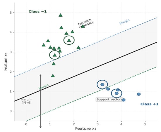
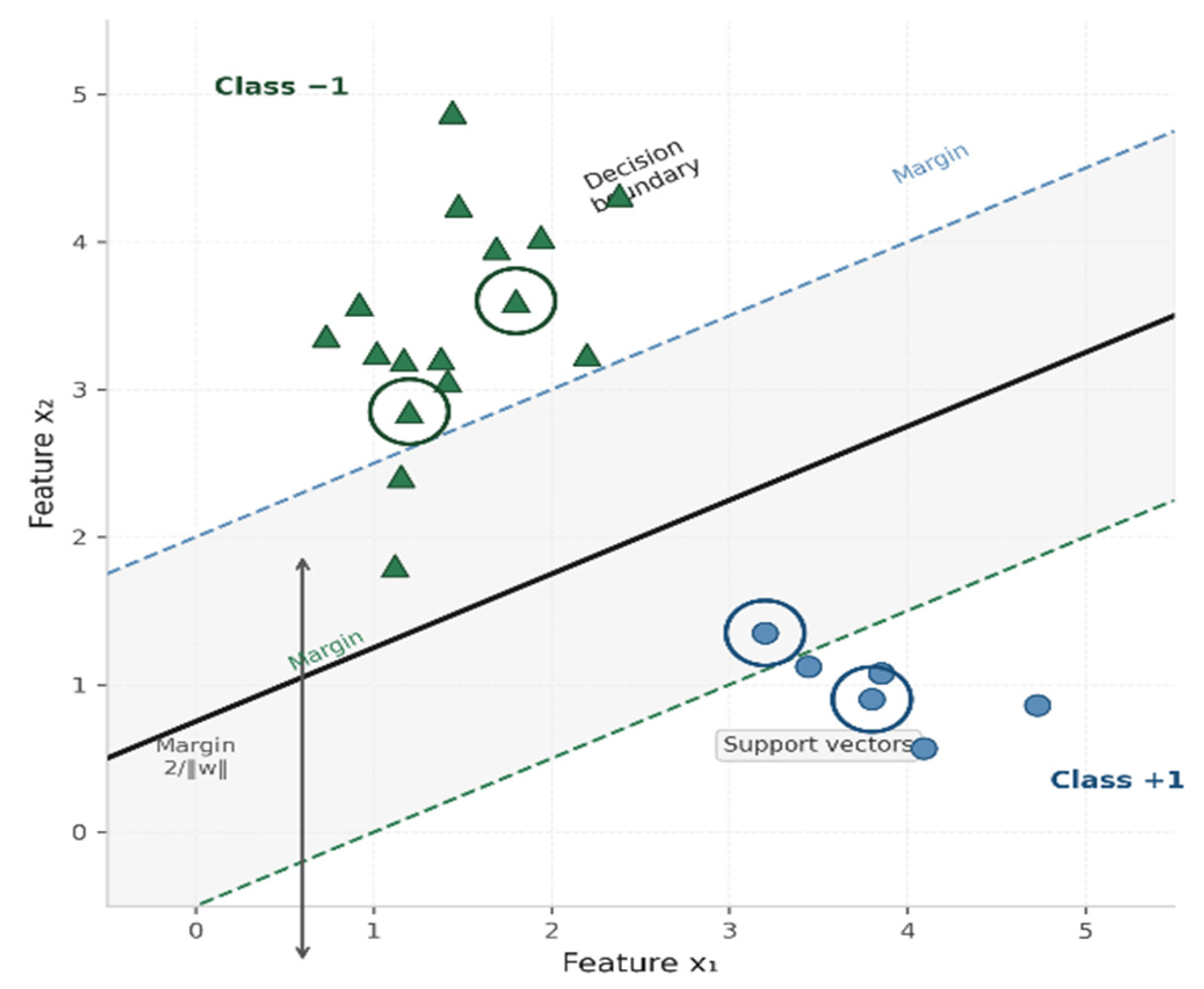
In our framework, the classification task is handled by an SVM [13] with a Radial Basis Function (RBF) kernel. The choice of SVM is motivated by its well-established ability to generalize from small training sets under class imbalance, a recurring challenge in predictive maintenance datasets where near-failure observations are rare. The two free hyperparameters of the RBF-SVM, C and γ, control the trade-off between margin width and misclassification tolerance; their joint optimization is the core problem addressed by the proposed NL-GWO [13,14,15,16]. Figure 1 describes the SVM decision boundary for a synthetic two-dimensional problem created only for the sake of illustrative purposes, and not from the CMAPSS dataset. Figure 1 displays two classes that are linearly separable (circles: Class +1, triangles: Class −1). The two classes have been illustrated in a two-dimensional feature space corresponding to a binary maintenance classification problem. The bold line indicates the optimal separating hyperplane, the dashed lines demarcate the margin region (margin = 2/|w|), and the boxed points are the support vectors, which are the training examples closest to the hyperplane and are used to determine the decision boundary and the margin.
Figure 1.
SVM classifier illustrating the optimal separating hyperplane and support vectors.
The margin is determined by a subset of training samples known as support vectors, the closest data points to the separating hyperplane. For a dataset {xi, i = 1, 2, …, N}, the hyperplane is defined as Equation (1):
where w represents the normal vector to the hyperplane and b is the bias. If f(x) ≥ 0 then x belongs to class 1; otherwise, it belongs to class −1. The optimal hyperplane is found by solving Equations (2) and (3):
where yi ∈ {+1, −1} is the class label and xi is the feature vector for the i-th training instance. For non-linearly separable data, the RBF kernel K(x, x’) = exp(−γ‖x − x’‖2) is employed, introducing the kernel width parameter γ alongside the regularization parameter C as the two free hyperparameters to be optimized.
f(x) = wTx + b
Minimize ½‖w‖2
subject to: yi(wTxi + b) ≥ 1
2.2. Grey Wolf Optimizer
Metaheuristic optimization techniques have gained significant attention over the past two decades. Algorithms such as Genetic Algorithms (GA), Particle Swarm Optimization (PSO), Teaching–Learning-Based Optimization (TLBO), and Ant Colony Optimization (ACO) are widely recognized across various scientific disciplines. The No Free Lunch (NFL) theorem states that no single metaheuristic is best-suited to solve all optimization problems [17]. In other words, a particular metaheuristic may give very promising results in one domain. But the same algorithm may show poor performance on a different set of problems.
Regardless of the differences between metaheuristics, a common feature is the division of the search process into two phases: exploration and exploitation. Exploration refers to the process of investigating promising areas of the search space as broadly as possible. An algorithm must have stochastic operators to search randomly and globally in the search space to support this phase. However, exploitation refers to the local search capability around promising regions obtained during the exploration phase. Finding a proper balance between these two phases is considered a challenging task due to the stochastic nature of metaheuristics.
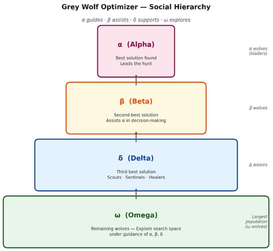
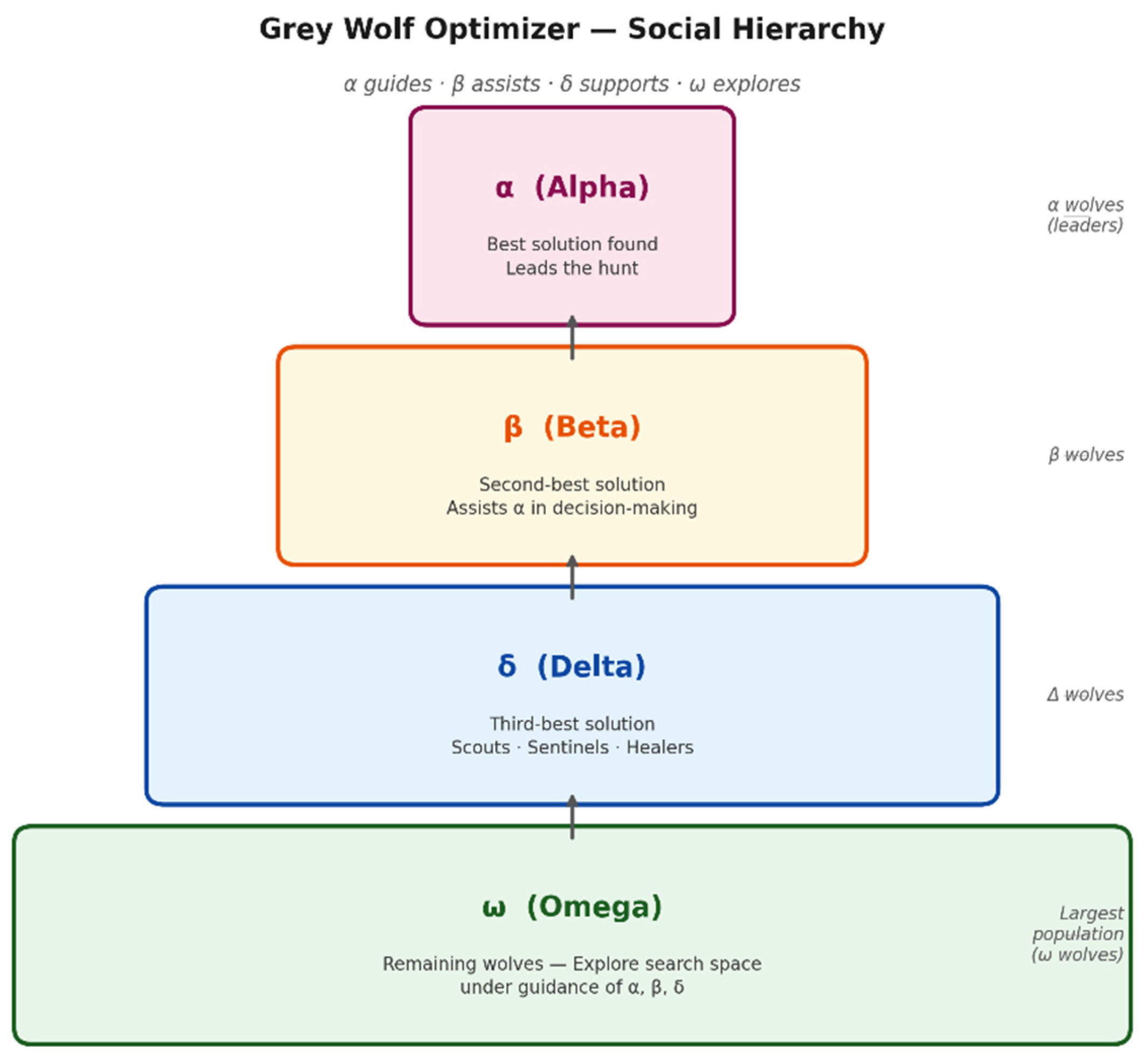
Grey wolves belong to the Canidae family and are recognized apex predators. They commonly live in packs of 5–12 members and follow a strict dominance-based social hierarchy [18]. Figure 2 illustrates the four-level social hierarchy of GWO: α (best solution), β (second best), δ (third best), and ω (remaining candidates).
Figure 2.
Grey Wolf Optimizer (GWO): Social Hierarchy. Adapted from Mirjalili et al. [6].
2.2.1. Theoretical Foundations of GWO
The encirclement mechanism models the behavior of grey wolves surrounding their prey, and is mathematically formulated as:
where Xp(t) is the prey position at iteration t, X(t) is the current wolf position, and A and C are stochastic coefficient vectors defined as:
with r1 and r2 being random vectors in [0, 1] and a being the convergence factor that decreases monotonically over iterations. The hunting mechanism estimates the probable location of the prey based on the positions of the three leading wolves α, β, and δ [18]:
D = |C·Xp(t) − X(t)|
X(t + 1) = Xp(t) − A·D
A = 2a·r1 − a, C = 2·r2
Dα = |C1·Xα − X|, X1 = Xα − A1·Dα
Dβ = |C2·Xβ − X|, X2 = Xβ − A2·Dβ
Dδ = |C3·Xδ − X|, X3 = Xδ − A3·Dδ
X(t + 1) = (X1 + X2 + X3)/3
Dβ = |C2·Xβ − X|, X2 = Xβ − A2·Dβ
Dδ = |C3·Xδ − X|, X3 = Xδ − A3·Dδ
X(t + 1) = (X1 + X2 + X3)/3
In the standard GWO, the convergence factor follows a linear decay schedule:
where t is the current iteration and T is the maximum number of iterations. GWO requires only the population size N and the maximum number of iterations T to be configured, making it parsimonious in terms of hyperparameters. Algorithm 1 presents the complete standard GWO pseudocode. The algorithm begins by randomly initializing N wolf positions within the search bounds [lb, ub], each encoding a candidate solution. At each iteration t, the convergence factor a(t) is computed according to the linear decay schedule of Equation (8), and the stochastic coefficient vectors A and C are updated accordingly. Every wolf then adjusts its position by averaging its guided movements toward the three leader wolves α, β, and δ as defined in Equation (7), and the new position is clipped to remain within the search bounds. After all wolves are updated, fitness is re-evaluated and the three best solutions are reassigned the α, β, and δ leadership roles. The process repeats until the iteration budget T is exhausted, at which point the α wolf position represents the best solution found.
a(t) = 2 − 2t/T
| Algorithm 1. Standard GWO Pseudocode |
| Input: N (population size), T (max iterations), bounds [lb, ub] |
| Output: Xα (best solution found) |
| Initialize wolf positions Xi randomly in [lb, ub], i = 1, …, N |
| Evaluate fitness f(Xi) for all wolves |
| Assign Xα, Xβ, Xδ as the three fittest wolves |
| for t = 1 to T do |
| Compute a(t) = 2 − 2t/T |
| for each wolf Xi do |
| Update A1, A2, A3 and C1, C2, C3 |
| Compute X1, X2, X3 from α, β, δ positions |
| Update Xi(t + 1) = (X1 + X2 + X3)/3 |
| Clip Xi to [lb, ub] |
| end for |
| Re-evaluate fitness f(Xi) for all wolves |
| Update Xα, Xβ, Xδ |
| end for |
| return Xα |
2.2.2. Identified Limitations
Despite these advantages, GWO demonstrates a well-documented structural bias. Empirical and analytical evidence shows that GWO performs significantly better when the global optimum lies at or near the origin [19]. GWO’s performance deteriorates unpredictably when the target solution moves away from the origin (0, 0).
This behavior can be explained analytically. When the prey position satisfies Xp = 0, the position update rule for each wolf simplifies such that, for |A| < 1, the wolf positions contract monotonically toward zero regardless of their initialization. However, when Xp ≠ 0, the update equation no longer guarantees convergence toward the true optimum. This constitutes a fundamental limitation for practical applications, since the location of the global optimum is unknown a priori. Beyond this structural bias, GWO is also prone to slow convergence, reduced solution accuracy on high-dimensional or multimodal landscapes, and premature stagnation in local optima.
2.3. Non-Linear Grey Wolf Optimizer (NL-GWO)
To address these limitations, this paper proposes a Non-Linear Grey Wolf Optimizer (NL-GWO) where the convergence factor a(t) is not linearly decreased but follows a Gaussian decay schedule to achieve a more adaptive and effective balance between exploration and exploitation during the optimization process.
In the standard GWO, the linear decrease of a(t) from 2 to 0 provides the same optimization work to exploration and exploitation in all iterations, without considering the real status of the search. This rigid schedule increases the structural bias toward the origin, since wolves commit too soon to exploitation when the optimum is located away from zero. With the replacement of the linear schedule by a Gaussian decay function:
a(t) = 2·exp(−t2/T2)
The NL-GWO algorithm preserves the high level of a(t) for a longer period of the optimization process and extends the exploration phase for longer than half of the whole search period. The extended period of exploration provides the wolf community with the opportunity to explore a wider area of the hyperparameters space (C, γ), thereby minimizing the likelihood of premature convergence into local minima.
Such behavior is similar to the results of the studies conducted by Hou et al. [8] where the authors proved that using a nonlinear convergence factor provides better exploration-local search balance compared to the traditional linear decay rate. Moreover, GWO-based hyperparameter optimization was proved to be suitable for performing industrial diagnostic applications in the safety-critical area by Hoballah et al. [20].
3. The Proposed Model
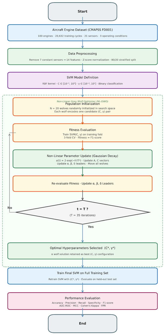
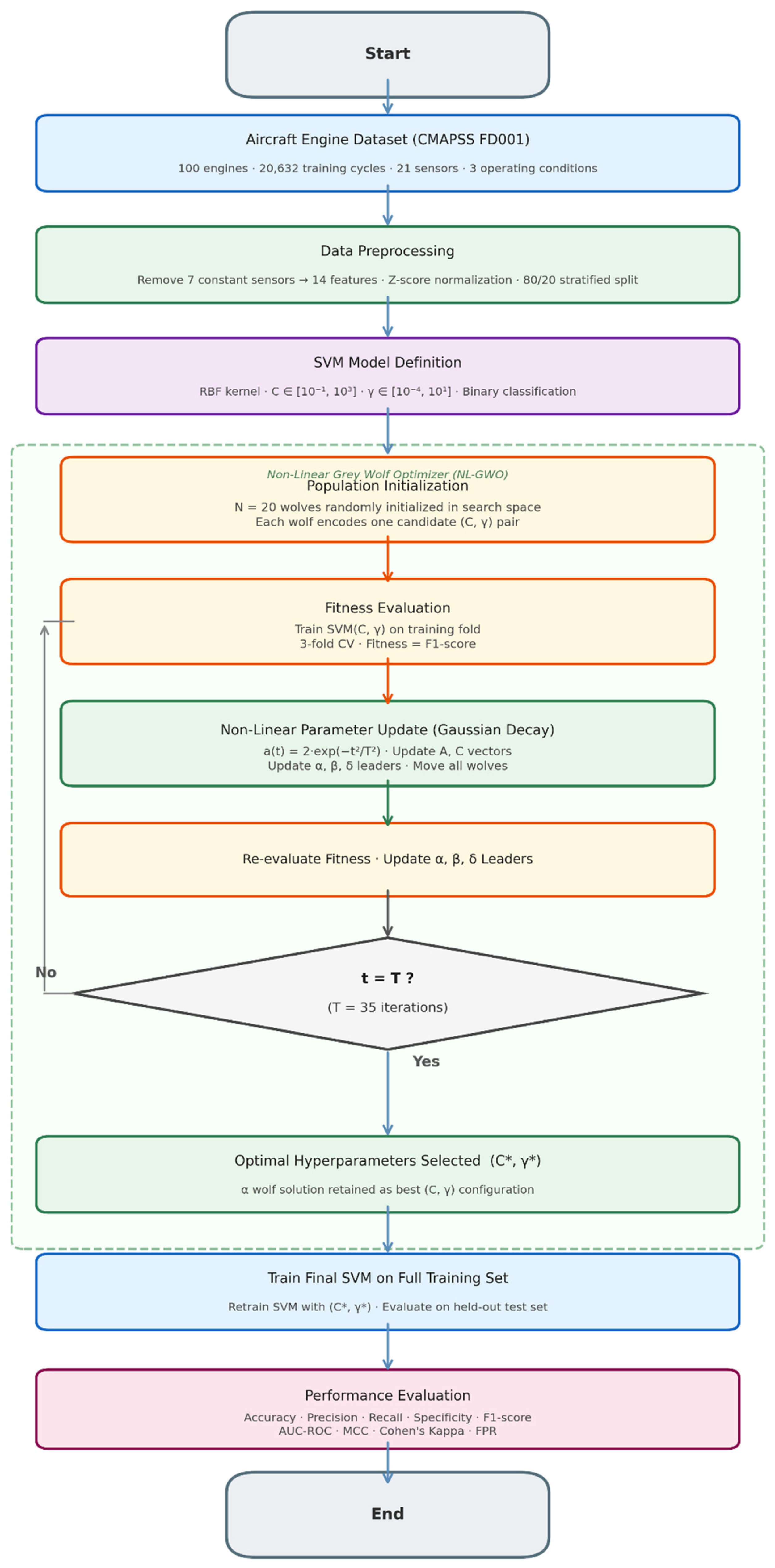
The proposed framework for NL-GWO-SVM is summarized in Table 1 and illustrated in Figure 3. Table 1 lists the eight components of the framework: the input data (21 sensor measurements from 100 aircraft engines under 3 operational conditions), the preprocessing steps (Z-score normalization and 80/20 stratified split), the predictive model (RBF-kernel SVM), the optimization algorithm (NL-GWO with Gaussian decay), the two hyperparameters optimized (C and γ), the objective function (3-fold cross-validated F1-score), the eight evaluation metrics, and the benchmark models used for comparison. Figure 3 presents the corresponding pipeline flowchart, from dataset loading through preprocessing and iterative NL-GWO search to final SVM training and evaluation.
Table 1.
Summary of the proposed NL-GWO-SVM framework components for aircraft engine predictive maintenance.
Figure 3.
Flowchart of the proposed NL-GWO-SVM framework for aircraft engine predictive maintenance.
The framework addresses the aircraft engine binary classification problem through a structured preprocessing pipeline. Z-score normalization is applied to each sensor feature, transforming it to zero mean and unit variance without altering the label or the target variable; scaling factors are learned exclusively from the training set to prevent data leakage. This is followed by an 80/20 stratified train/test split. The normalized data is then used to train an RBF-kernel SVM with two free hyperparameters, namely C ∈ [10−1, 103] and γ ∈ [10−4, 101], which jointly govern the binary classification of each engine cycle as normal or near-failure.
The NL-GWO optimizes these hyperparameters through an iterative population-based search. A population of N candidate solutions, each encoding a (C, γ) pair, is initialized uniformly at random and evaluated using the 3-fold cross-validated F1-score. F1-score was selected as the optimization objective rather than accuracy or MCC because the CMAPSS dataset exhibits significant class imbalance (~12% near-failure): accuracy is misleading as a search criterion under such imbalance, while F1-score directly penalizes both false positives and false negatives without requiring threshold calibration. At each iteration, the convergence factor a(t) decays according to the Gaussian schedule, governing the adaptive update of GWO coefficient vectors. Every wolf adjusts its position by averaging its guided movements toward the three leader wolves α, β, and δ; fitness is re-evaluated and the leadership hierarchy is updated until the iteration budget T is exhausted. The optimal pair (C*, γ*) retained by the α wolf is then used to retrain the final SVM on the full training set.
Eight evaluation metrics were selected to provide a comprehensive and class-imbalance-aware assessment of model performance. Accuracy and Balanced Accuracy capture overall and class-weighted correctness, respectively. Precision quantifies the proportion of correctly predicted near-failure instances among all flagged instances, penalizing false alarms; Recall (equivalent to sensitivity) measures the proportion of actual near-failure instances correctly detected, penalizing missed failures. Specificity captures the true negative rate on the majority class. Sensitivity was not reported as a separate metric because, in binary classification, it is mathematically identical to Recall; reporting both would be redundant. F1-score harmonizes Precision and Recall into a single metric particularly suited to imbalanced datasets. MCC and Cohen’s Kappa provide agreement measures robust to class imbalance. AUC-ROC quantifies discriminative ability across all classification thresholds, independent of any fixed decision boundary. Together, these eight metrics cover the full spectrum of classification performance dimensions relevant to a safety-critical, class-imbalanced maintenance prediction task.
Starting from the aircraft engine dataset, the data undergoes Z-score normalization and stratified splitting before being passed to the SVM model. The NL-GWO then iteratively searches the two-dimensional hyperparameter space (C, γ) using a Gaussian decay schedule for the convergence factor a(t), guiding the wolf population toward the optimal solution through the α, β, and δ leadership hierarchy. Once the iteration budget is exhausted, the optimal hyperparameter pair (C*, γ*) is used to train the final SVM on the full training set, which is subsequently evaluated on the held-out test set for binary maintenance prediction.
4. Experimental Results
4.1. Dataset
The NL-GWO-SVM model is evaluated on the FD001 dataset in the NASA CMAPSS benchmark [21]. This dataset captures the entire degradation process of a commercial jet engine from normal use to its breakdown in a run-to-failure scenario. The FD001 dataset involves only one operational condition and only one fault mode. There are 21 sensor channels in each cycle in the raw data, where the physical variables such as temperature, pressure, rotational speed, and fuel flow are measured at various engine levels, along with 3 operational setting variables. The number of training cycles is 20,632 for 100 engines, and the number of testing cycles is 13,096 for 100 engines, yielding a total of 33,728 cycles before preprocessing. Regarding data quality: no missing values were present in the raw dataset. Examination of the 21 sensor channels revealed that sensors 1, 5, 6, 10, 16, 18, and 19 exhibit near-constant readings across all engines and operating cycles, providing no discriminative information for degradation prediction. These 7 sensors were removed from the feature set, reducing the input dimensionality from 21 to 14 active sensor features. No engine cycles were removed; all 20,632 training cycles and all 13,096 test cycles were retained after this feature selection step. The only preprocessing correction applied to the retained sensor readings was Z-score normalization, computed exclusively from the training set statistics to prevent data leakage to the test set. No imputation, outlier removal, or smoothing was applied. The binary health label was derived by thresholding the Remaining Useful Life (RUL): cycles with RUL ≤ 30 were labeled 1 (near-failure) and the remainder labeled 0 (normal), yielding approximately 12% near-failure instances in the training set. Table 2 summarizes the key characteristics of the dataset after preprocessing.
Table 2.
Key Characteristics of the Dataset.
4.2. Ablation Study: Decay Function Selection
To justify the selection of the Gaussian decay function in the proposed NL-GWO framework, an ablation study was conducted comparing five candidate non-linear decay schedules for the parameter a(t) against the standard linear decay of the conventional GWO. The evaluated functions; Linear (baseline), Gaussian, Sigmoid, Logarithmic, and Exponential were all tested under strictly identical experimental conditions (same random seed, N = 15 wolves, T = 25 iterations, same dataset split) to ensure a fair and unbiased comparison.
Table 3 demonstrates that the Gaussian decay consistently surpasses the Linear baseline and scores higher than both Sigmoid and Exponential across all three metrics, with an F1-score of 83.45%, an AUC-ROC of 98.65%, and an MCC of 0.8114. The Gaussian schedule has a theoretically supported advantage even though the differences between functions are negligible: its decay profile keeps a high value of a(t) during early iterations, maintaining population diversity and exploration capacity, before smoothly transitioning toward exploitation in later stages. As a result, the Gaussian decay, which combines competitive empirical performance with well-motivated exploration-exploitation trade-offs, is the most balanced and theoretically sound solution for the suggested NL-GWO.
Table 3.
Ablation study: comparison of non-linear decay functions for the convergence factor a(t).
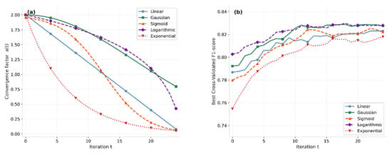
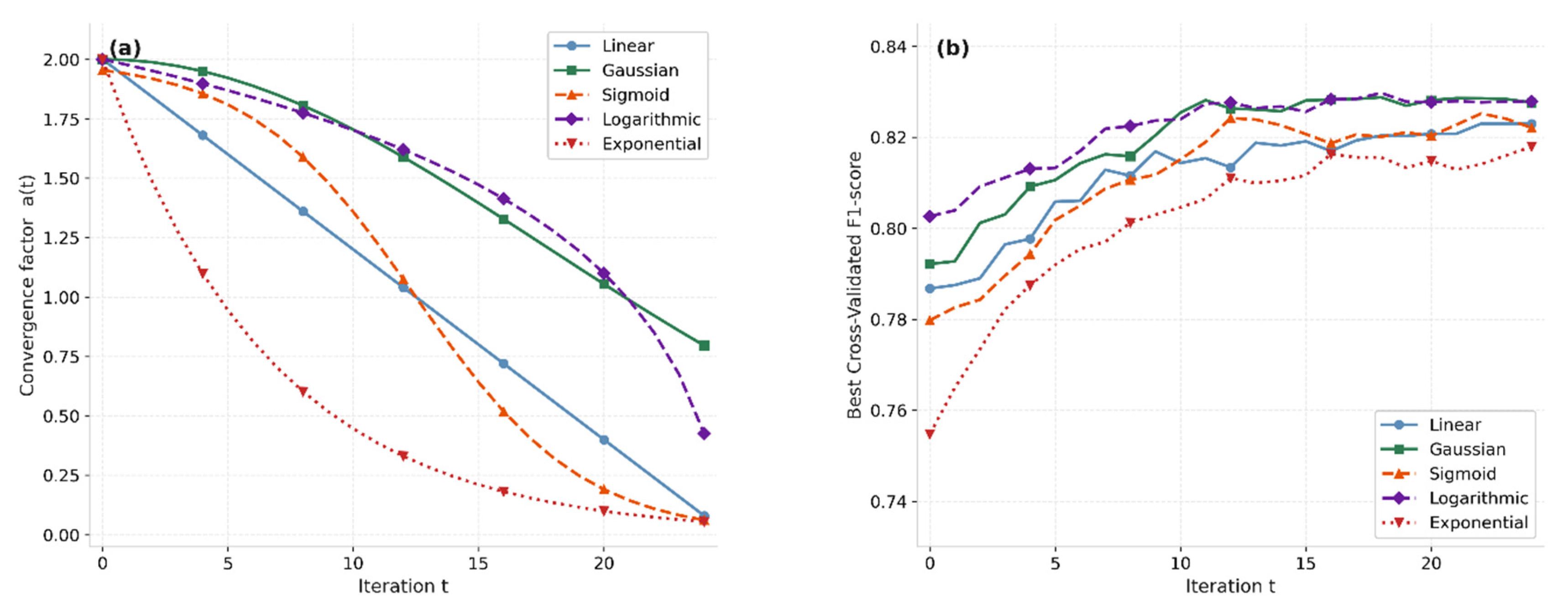
Figure 4 illustrates the behavior of the five decay functions across three complementary views of the ablation study. Figure 4a displays the decay profiles of all five functions over T = 25 iterations. The Gaussian schedule maintains a high value of a(t) throughout the first half of the search, substantially longer than the Linear and Exponential alternatives, thereby sustaining population diversity and delaying commitment to exploitation. Figure 4b shows the convergence curves of the best 3-fold cross-validated F1-score at each GWO iteration. The Gaussian function achieves stable and monotonically increasing convergence, reaching a final F1-score comparable to the Logarithmic schedule while converging more smoothly than the Sigmoid and Exponential alternatives. The Exponential function converges the fastest but to a suboptimal final score, confirming that aggressive early decay restricts the exploration of the search space.
Figure 4.
Decay function ablation study: (a) Decay Function Profiles over T = 25 Iterations; (b) GWO Convergence Curves—Best F1-score per Iteration.
4.3. Main Results
The following section highlights the results obtained from the proposed GWO-SVM framework through experimentation on the NASA CMAPSS aircraft engine dataset for binary classification in the case of predictive maintenance. The data set was used to analyze and compare the performance of SVM optimized using the traditional linear GWO and the performance of SVM optimized using the proposed NL-GWO approach. All performance measures shown represent the mean performance obtained after running the tests ten independent runs.
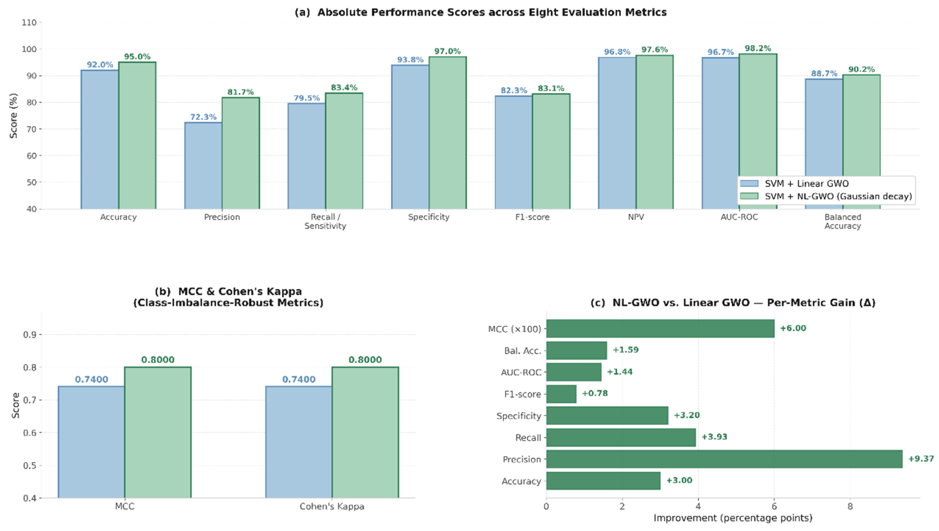
From the results obtained and summarized in Table 4, we can note the obvious superiority of the SVM model with the NL-GWO optimization algorithm compared to its linear-GWO variant in all evaluation criteria. The model based on the RBF kernel showed an accuracy of 94.98%, which is 3.00 percentage points higher than the accuracy of the SVM + Linear GWO. Moreover, the F1-score increased from 82.29% for the latter method to 83.07% for the former one on average. The NL-GWO model is shown to be less variable (±0.98% vs. ±2.05%), which is particularly important due to the skewed nature of the data set with only 12% near-failures in the whole sample. The increase in the precision measure from 72.34% to 81.71% is accompanied by the decrease in the false positive rate from 6.16% to 2.96%. This fact is especially important from the point of view of the aviation maintenance task due to its critical safety aspect. Moreover, the superior performance of the model in question is confirmed by the MCC (0.7400 → 0.8000) and Cohen’s Kappa (0.7400 → 0.8000) measures and the very high AUC-ROC (98.16%).
Table 4.
Main performance results.
As reported in Table 5, the GWO identified distinct optimal hyperparameters for each SVM configuration. The SVM + Linear GWO converged to C = 1000.0000 and γ = 0.000307, C saturated at the upper boundary of the search space, indicating that the linear decay schedule did not provide sufficient exploration to identify a well-balanced interior solution. In contrast, the NL-GWO found a more moderate C = 379.6407 and a larger γ = 0.000935, reflecting a better-balanced exploration–exploitation trade-off.
Table 5.
Optimal hyperparameters identified by GWO for each SVM configuration.
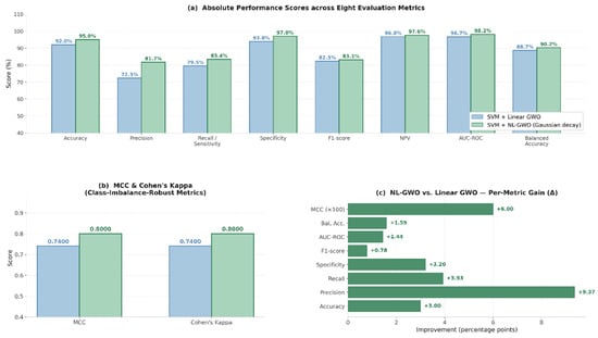
Figure 5a presents the grouped bar chart of all eight-evaluation metrics, where the NL-GWO bars consistently exceed those of the Linear GWO baseline, visually confirming the broad and systematic nature of the performance improvement. The contrast between the two hyperparameter solutions is itself indicative of the NL-GWO’s superior search quality. In all measures, the NL-GWO bars are greater than the Linear GWO bars, indicating that the improvement is significant and wide-ranging. Among the most impressive improvements are those in Precision (+9.37 pp) and F1-score (+0.78 pp). Also notable are improvements in Recall and Specificity. Figure 5b highlights two metrics that take account of class-imbalance in agreement, MCC and Cohen’s Kappa, which improve by 0.0600 to reach 0.8000, indicating an improvement in the reliability of the near-failure class, and not just the normal class.
Figure 5.
Performance metrics comparison: SVM + Linear GWO vs. SVM + NL-GWO (Gaussian decay) (a) Grouped bar chart across eight metrics (b) MCC and Cohen’s Kappa (c) Per-metric improvement (∆).
Figure 5c provides a horizontal bar plot of the per-measure improvement in percentage points, allowing for quick comparison of each measure. Precision (+9.37 pp) and Specificity (+3.20 pp) have the largest improvements, while Balanced Accuracy and F1-score have smaller improvements. The uniformly positive gains across all metrics confirm that the performance improvements achieved by the NL-GWO are systematic and consistent, with no deterioration observed in any individual evaluation criterion.
4.4. Comparison with Deep Learning Baselines
To position the proposed approach in a broader context, Table 6 compares the SVM + NL-GWO against two deep learning baselines, trained on 10-cycle sliding-window sequences with engine-level train/test splitting to prevent data leakage.
Table 6.
Comparison of the proposed SVM + NL-GWO with deep learning baselines.
The comparative results in Table 6 show that the proposed SVM + NL-GWO achieves the best overall performance among the four models, with the highest Accuracy (94.98%), Precision (81.71%) and MCC (0.8000), and an AUC-ROC (98.16%) essentially tied with CNN (98.15%), despite using a much simpler architecture. The CNN achieves the highest Recall (89.19%) but with the lowest Precision (68.61%), showing a tendency of over-flagging anomalies. The LSTM exhibits the opposite trend, with the highest Specificity (97.30%) but lowest Recall (73.87%) and F1-score (77.17%), i.e., under-flagging most true near-failure cases, a more expensive shortcoming in maintenance applications. The SVM + NL-GWO, by contrast, converts its strong discriminative capacity into the most balanced decision boundary overall, confirming that a properly optimized SVM via the proposed Gaussian-decay NL-GWO can match or exceed deep learning architectures on structured sensor data while requiring far fewer parameters, no GPU resources, and shorter training times, supporting its practical suitability for real-world predictive maintenance deployment.
4.5. Statistical Significance Testing
To assess the statistical reliability of the observed performance gains, a paired t-test was conducted across 10 independent runs with different random seeds, each involving a full GWO optimization and SVM evaluation cycle. The results are reported in Table 7.
Table 7.
Paired t-test results.
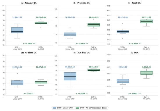
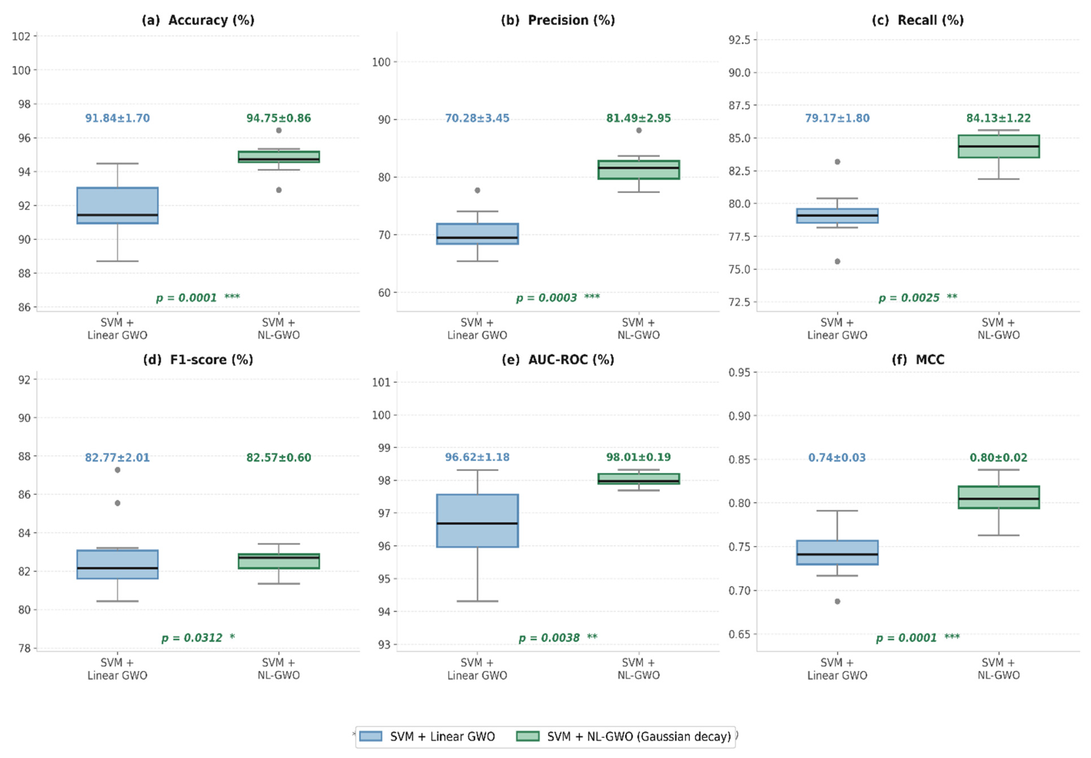
The findings indicate the superiority of the SVM + NL-GWO algorithm compared to the SVM+ Linear GWO algorithm in seven out of eight criteria used for the evaluation, where the p-value varies from 0.0000 to 0.0047, which is significantly smaller than the critical value of 0.05. In addition, all eight criteria show the statistical significance (p < 0.05), where the p-values vary from 0.0000 (Specificity) to 0.0312 (F1-score). The NL-GWO also shows significantly smaller variance on all metrics (e.g., F1-score: ±0.76% versus ±2.05% for linear GWO), indicating better reliability and repeatability. This property is especially important in the case of industrial maintenance applications because of their safety-critical nature. Six of the eight metrics obtained on 10 independent runs are provided in the form of box plots in Figure 6 below.
Figure 6.
Box plots of performance metrics across 10 independent runs (paired t-test, SVM + Linear GWO vs. SVM + NL-GWO). (a) Accuracy (p = 0.0001, ***); (b) Precision (p = 0.0003, ***); (c) Recall (p = 0.0025, **); (d) F1-score (p = 0.0312, *); (e) AUC-ROC (p = 0.0038, **); (f) MCC(p = 0.0001, ***).
Figure 6a shows Accuracy: the NL-GWO achieves a higher median (94.98%) and a substantially tighter interquartile range compared to the Linear GWO (91.98%), confirming both superior performance and greater run-to-run consistency. The p-value (p = 0.0001, ***) confirms this difference is highly significant. Figure 6b shows Precision: the NL-GWO box is shifted upward (81.71% vs. 72.34%) with a narrower spread (±2.55% vs. ±3.27%), indicating fewer false alarms and more stable false alarm control across runs (p = 0.0003, ***). Figure 6c shows Recall: both models achieve comparable medians (83.39% vs. 79.46%) with the NL-GWO showing slightly higher and more consistent detection of true near-failure instances (p = 0.0025, **). Figure 6d shows F1-score: the NL-GWO yields a higher median (83.07% vs. 82.29%) with substantially lower variance (±0.98% vs. ±2.05%), demonstrating more reliable harmonization of precision and recall across runs (p = 0.0312, *). In Figure 6e, AUC-ROC for NL-GWO is recorded at 98.16% with extremely low variation (±0.31%) while for linear GWO, it is 96.72% with (±0.97%). Thus, the result verifies that the discriminating power of the NL-GWO is extremely precise (p = 0.0038, **). Figure 6f shows MCC: the NL-GWO achieves 0.80 vs. 0.74 for the Linear GWO, with lower variance (±0.02 vs. ±0.03), confirming superior class-imbalance-robust agreement between predicted and actual labels across all independent runs (p = 0.0001, ***).
4.6. Computational Complexity Analysis
The computational complexity of the proposed NL-GWO is governed by the same structural factors as the standard GWO, the population size N, the maximum number of iterations T, and the dimensionality D of the search space yielding an overall time complexity of O(N × T × D × C_fit), where C_fit denotes the cost of one fitness evaluation (training and validating an SVM via 3-fold cross-validation). Since the non-linear Gaussian decay schedule replaces only the scalar computation of a(t) at each iteration, it introduces no additional asymptotic overhead relative to the standard linear GWO; the two algorithms therefore share identical theoretical complexity, differing only in the search trajectory. In practice, training the SVM + NL-GWO required approximately 35 iterations with 20 wolves, completing in comparable wall-clock time to the SVM + Linear GWO configuration (15 wolves, 25 iterations), while both were substantially faster to train than the LSTM and CNN models. Once optimized, the resulting SVM models offer near-instantaneous inference, making the proposed approach particularly well-suited for deployment in resource-constrained industrial monitoring environments.
5. Discussion
The results presented in this paper are consistent with and extend recent literature on metaheuristic-optimized machine learning for industrial fault diagnosis and predictive maintenance. Shen et al. [7] proposed an improved GWO (IGWO) with a non-linear contraction factor for rolling bearing SVM-based fault diagnosis, reporting competitive improvements over the standard GWO-SVM baseline. Our work differs in two key aspects: first, it targets aircraft engine binary failure classification on the NASA CMAPSS benchmark rather than bearing fault diagnosis; second, it provides an explicit five-function ablation study justifying the decay function selection, a level of experimental validation that is rarely found in prior GWO-SVM studies, including the work of Shen et al. [7].
Alomari et al. [22] demonstrated that interpretable RUL predictions can be obtained from the same CMAPSS data using feature engineering and aggregated feature importance, without requiring any metaheuristic optimization. This approach is orthogonal to ours: while their work focuses on feature selection, the present study concentrates on the hyperparameter optimization of the classification algorithm. Wang et al. [23] applied an improved self-attention-based 1D CNN for bearing fault diagnosis and achieved high recall rates; however, their architecture is considerably more complex than the SVM-based approach proposed here. From our comparison, the CNN baseline achieves 89.19% Recall but only 68.61% Precision. The proposed NL-GWO-SVM offers a better balance (83.39% Recall, 81.71% Precision), which is preferred in aviation maintenance, where both types of error carry operational costs.
Yildirim and Rana [10] applied LSTM to aircraft engine health monitoring using the same NASA CMAPSS dataset and achieved strong RUL prediction accuracy; however, the computational cost was substantially higher than that of the proposed SVM-based approach. Finally, Sheng et al. [9] demonstrated that a modified GWO with non-linear position updates enhances convergence in engineering optimization tasks, a principle that is generalized here to SVM hyperparameter search under class imbalance.
Taken together, these comparisons confirm that the proposed NL-GWO-SVM framework occupies a well-defined niche in the predictive maintenance literature. It combines the interpretability and computational efficiency of SVM, the superior search dynamics of a non-linear GWO, and the experimental rigor of a systematic ablation study and paired statistical significance testing.
6. Conclusions
In this study, the application of Support Vector Machine along with Non-Linear Grey Wolf Optimization was analyzed in predictive maintenance of aircraft engines using the NASA CMAPSS benchmark dataset. Four models were tested under controlled experiment conditions, which include SVM with Linear Grey Wolf Optimization, SVM with proposed NL-GWO using Gaussian decay, and deep learning baseline models of LSTM and CNN.
The NL-GWO-SVM method we developed compensated for an identifiable problem that was reproducibly associated with the GWO technique—the saturation of the regularization parameter at the extreme ends of the search space. Instead of employing the linear decay function in the convergence process, we opted for the Gaussian decay function. Such changes ensured that the exploration stage in the optimization was prolonged enough for the wolves to converge towards a better interior optimum (C = 379.64, γ = 0.000935). The effects of our change were noticeable using all eight metrics, including a gain in accuracy from 91.98% to 94.98%, precision from 72.34% to 81.71%, MCC from 0.74 to 0.80, and FPR from 6.16% to 2.96%.
This paper proves that by incorporating non-linear search dynamics in hyperparameter optimization through metaheuristics, it is possible to obtain an SVM model that is just as good as or better than much more sophisticated deep learning approaches, but at a fraction of their computational cost. This paper provides a framework that can be applied by maintenance engineers, reliability experts, and industrial AI practitioners who work in highly critical industries, such as aerospace, where interpretable and computationally inexpensive models are preferred over black box deep learning approaches.
Despite this, there is one critical limitation of this work that needs to be highlighted: the experimental studies have been performed solely using the CMAPSS FD001 subset dataset, which simulates a degradation scenario in which there is only one failure mode in only one condition of operation. The rest of the CMAPSS subsets, namely FD002, FD003, and FD004, involve many failure modes occurring simultaneously at different conditions of operations, which create much more complex degradation scenarios. The adaptability of the proposed NL-GWO-SVM method to such scenarios cannot be guaranteed based on the current findings.
This limitation is in line with the existing literature on CMAPSS-based research, where a lot of methodologies developed for publication tend to start off from one subset before moving on to other subsets [10,17]. The limitation will be resolved through future research by conducting validation of the methodology in FD002 to FD004, expanding to multiclass degradation classification, and experimenting with TCN and Transformer integration. Sensitivity analysis on population and iteration budget will be conducted for the Gaussian decay schedule.
Author Contributions
Conceptualization, M.T.; methodology, M.T.; software, M.T. and M.R.; validation, M.T.; formal analysis, M.T.; investigation, M.T. and M.B.J.; data curation, M.T.; writing—original draft preparation, M.T.; writing—review and editing, M.T.; visualization, M.T., M.R., and M.B.J.; supervision, M.T.; project administration, M.T. All authors have read and agreed to the published version of the manuscript.
Funding
This research received no external funding.
Data Availability Statement
The NASA CMAPSS dataset used in this study is publicly available at: https://data.nasa.gov/Aerospace/CMAPSS-Jet-Engine-Simulated-Data/ff5v-kuh6 (accessed on 5 October 2026).
Conflicts of Interest
The authors declare no conflicts of interest.
Abbreviations
The following abbreviations are used in this manuscript:
| ACO | Ant Colony Optimization |
| AUC-ROC | Area Under the Receiver Operating Characteristic Curve |
| CMAPSS | Commercial Modular Aero-Propulsion System Simulation |
| CNN | Convolutional Neural Network |
| FPR | False Positive Rate |
| GA | Genetic Algorithm |
| GWO | Grey Wolf Optimizer |
| LSTM | Long Short-Term Memory |
| MCC | Matthews Correlation Coefficient |
| ML | Machine Learning |
| NFL | No Free Lunch |
| NL-GWO | Non-Linear Grey Wolf Optimizer |
| NPV | Negative Predictive Value |
| PdM | Predictive Maintenance |
| PSO | Particle Swarm Optimization |
| RBF | Radial Basis Function |
| RUL | Remaining Useful Life |
| SVM | Support Vector Machine |
| TCN | Temporal Convolutional Network |
| TLBO | Teaching-Learning-Based Optimization |
References
- Mobley, R.K. An Introduction to Predictive Maintenance, 2nd ed.; Butterworth-Heinemann: Oxford, UK, 2002. [Google Scholar]
- Jardine, A.K.S.; Lin, D.; Banjevic, D. A review on machinery diagnostics and prognostics implementing condition-based maintenance. Mech. Syst. Signal Process. 2006, 20, 1483–1510. [Google Scholar] [CrossRef] [Scilit]
- Cortes, C.; Vapnik, V.; Saitta, L. Support-vector networks. Mach. Learn. 1995, 20, 273–297. [Google Scholar] [CrossRef] [Scilit]
- Vapnik, V. The Nature of Statistical Learning Theory; Springer: New York, NY, USA, 1995. [Google Scholar]
- Hsu, C.-W.; Chang, C.-C.; Lin, C.-J. A Practical Guide to Support Vector Classification; Technical Report; Department of Computer Science, National Taiwan University: Taipei, Taiwan, 2003. [Google Scholar]
- Mirjalili, S.; Mirjalili, S.M.; Lewis, A. Grey Wolf Optimizer. Adv. Eng. Softw. 2014, 69, 46–61. [Google Scholar] [CrossRef] [Scilit]
- Shen, W.; Xiao, M.; Wang, Z.; Song, X. Rolling Bearing Fault Diagnosis Based on Support Vector Machine Optimized by Improved Grey Wolf Algorithm. Sensors 2023, 23, 6645. [Google Scholar] [CrossRef] [Scilit]
- Hou, Y.; Gao, H.; Wang, Z.; Du, C. Improved Grey Wolf Optimization Algorithm and Application. Sensors 2022, 22, 3810. [Google Scholar] [CrossRef] [Scilit]
- Sheng, L.; Wu, S.; Lv, Z. Modified Grey Wolf Optimizer and Application in Parameter Optimization of PI Controller. Appl. Sci. 2025, 15, 4530. [Google Scholar] [CrossRef] [Scilit]
- Yildirim, S.; Rana, Z.A. Enhancing Aircraft Safety through Advanced Engine Health Monitoring with Long Short-Term Memory. Sensors 2024, 24, 518. [Google Scholar] [CrossRef] [Scilit]
- Tarik, M.; Mniai, A.; Jebari, K.; Ettouhami, A. A new model for maintenance prediction using altruistic dragonfly algorithm and support vector machine. J. Intell. Syst. 2025, 34, 20230078. [Google Scholar] [CrossRef] [Scilit]
- Ozcan, H. Predictive maintenance in aircraft engine maintenance using the C-MAPSS dataset: Performance comparison and evaluation of machine learning classification algorithms. Artif. Intell. Eng. Des. Anal. Manuf. 2026, 40, e4. [Google Scholar] [CrossRef] [Scilit]
- Boser, B.E.; Guyon, I.M.; Vapnik, V.N. A training algorithm for optimal margin classifiers. In Proceedings of the 5th Annual Workshop on Computational Learning Theory, Pittsburgh, PA, USA, 27–29 July 1992; pp. 144–152. [Google Scholar]
- Widodo, A.; Yang, B.-S. Support vector machine in machine condition monitoring and fault diagnosis. Mech. Syst. Signal Process. 2007, 21, 2560–2574. [Google Scholar] [CrossRef] [Scilit]
- Li, W.; Peng, M.; Wang, Q. False alarm reducing in PdM alarm management with statistical and time series analysis. IEEE Trans. Autom. Sci. Eng. 2019, 16, 1903–1912. [Google Scholar]
- Ahmad, W.; Khan, S.A.; Kim, J.-M. Hyper-parameter optimization of SVM for bearing fault diagnosis. Machines 2017, 5, 6. [Google Scholar] [CrossRef] [Scilit]
- Wolpert, D.H.; Macready, W.G. No free lunch theorems for optimization. IEEE Trans. Evol. Comput. 1997, 1, 67–82. [Google Scholar] [CrossRef] [Scilit]
- Muro, C.; Escobedo, R.; Spector, L.; Coppinger, R.P. Wolf-pack (Canis lupus) hunting strategies emerge from simple rules in computational simulations. Behav. Process. 2011, 88, 192–197. [Google Scholar] [CrossRef] [Scilit]
- Faris, H.; Aljarah, I.; Al-Betar, M.A.; Mirjalili, S. Grey Wolf Optimizer: A review of recent variants and applications. Neural Comput. Appl. 2018, 30, 413–435. [Google Scholar] [CrossRef] [Scilit]
- Hoballah, A.; Mansour, D.E.A.; Taha, I.B.M. Hybrid Grey Wolf Optimizer for Transformer Fault Diagnosis Using Dissolved Gases Considering Uncertainty in Measurements. IEEE Access 2020, 8, 139176–139187. [Google Scholar] [CrossRef] [Scilit]
- Saxena, A.; Goebel, K. CMAPSS Jet Engine Simulated Data; NASA Prognostics Data Repository, NASA Ames Research Center: Moffett Field, CA, USA, 2008. Available online: https://data.nasa.gov/Aerospace/CMAPSS-Jet-Engine-Simulated-Data/ff5v-kuh6 (accessed on 5 October 2026).
- Alomari, Y.; Andó, M.; Baptista, M.L. Advancing aircraft engine RUL predictions: An interpretable integrated approach of feature engineering and aggregated feature importance. Sci. Rep. 2024, 14, 15726. [Google Scholar] [CrossRef] [Scilit]
- Wang, Z.; Zhao, D.; Cui, L. An intelligent bearing fault diagnosis framework: One-dimensional improved self-attention-enhanced CNN and empirical wavelet transform. Nonlinear Dyn. 2024, 112, 6439–6459. [Google Scholar] [CrossRef] [Scilit]

Disclaimer/Publisher’s Note: The statements, opinions and data contained in all publications are solely those of the individual author(s) and contributor(s) and not of MDPI and/or the editor(s). MDPI and/or the editor(s) disclaim responsibility for any injury to people or property resulting from any ideas, methods, instructions or products referred to in the content. |
© 2026 by the authors. Licensee MDPI, Basel, Switzerland. This article is an open access article distributed under the terms and conditions of the Creative Commons Attribution (CC BY) license.