


Abstract
This paper introduces a computationally efficient method for identifying the orientation of objects with diverse geometries and is compared with other popular image processing approaches. The proposed method estimates object orientation by averaging multiple extreme boundary points located at opposite sides of the detected object contour, thereby reducing the sensitivity of the orientation estimation to individual boundary-point perturbations. Unlike learning-based approaches that require model training, the proposed method operates directly on the detected object contour. Across the complete set of 1870 images, it achieved a sample-weighted pooled mean angular error of 16.17° and a mean execution time of 34.28 μs, while the macro-average angular error across the five datasets was 18.404°. The proposed method may be suitable for computationally constrained applications with morphology-dependent accuracy constraints. The proposed technique is evaluated against five established orientation estimation methods: Ellipse Fitting, Principal Component Analysis (PCA), Minimum Area Rectangle, Morphological skeleton, and Hough Transform. Although Hough Transform achieved higher overall angular accuracy, the proposed method required substantially less execution time. Extensive experiments were conducted on 1870 images of various fish species and plant leaves, covering a wide range of resolutions and structural complexities. Experimental results show that acceptable accuracy is achieved while maintaining a significantly lower computational execution time. In shape alignment applications based on Ensemble of Regression Trees (ERT), orientation estimation error within ±20° is typically acceptable; thus, the proposed method can be exploited.
1. Introduction
Accurate orientation estimation of two-dimensional objects constitutes a fundamental problem in computer vision, pattern recognition, robotics, and biological image analysis. The determination of the dominant axis of an object is essential in applications such as robotic manipulation and navigation [1], morphological analysis of biological specimens [2], automated species classification in ecological monitoring systems [3], medical image interpretation [4], and industrial production lines [5]. Despite decades of research, robust orientation estimation remains challenging when objects exhibit irregular shapes, concavities, partial occlusions, or high contour variability.
Classical approaches to orientation estimation are primarily based on second-order statistical moments and geometric fitting. Principal Component Analysis (PCA) is widely used due to its simplicity and computational efficiency, extracting the dominant eigenvector of the covariance matrix of contour points to determine the principal direction [6,7]. Similarly, Ellipse Fitting methods approximate the contour with a conic section and compute the orientation of the major axis [8]. These techniques perform well when objects exhibit near-elliptical symmetry or uniform mass distribution. However, their performance deteriorates significantly in the presence of asymmetric protrusions, non-uniform thickness, or serrated boundary characteristics commonly observed in biological objects such as fish and leaves.
More advanced contour-based descriptors have been proposed to address these limitations. Fourier descriptors represent closed contours in the frequency domain, enabling rotation-invariant shape analysis [9]. Shape context descriptors capture local geometric distributions for matching and recognition tasks [10]. Curvature-based representations and geodesic metrics further enhance discrimination power in complex shapes [11]. While these approaches improve robustness in recognition scenarios, they are often computationally demanding and not specifically optimized for direct orientation estimation.
Transform-based methods such as the Hough Transform have also been extensively applied to detect dominant linear structures within images [12]. These computationally expensive techniques depend heavily on threshold selection and accumulator resolution, making them sensitive to noise. Similarly, skeletonization and medial axis transforms provide structural representations of shapes [13,14], but iterative morphological operations introduce significant computational overhead and may amplify segmentation artifacts.
Another widely used geometric approach is the minimum area bounding rectangle (MinAreaRect), which determines the orientation of the rectangle with minimal area enclosing the contour of the object under interest [15]. Despite the efficiency of this method, instability may be exhibited when multiple near-optimal bounding rectangles exist, especially for objects with different body shapes.
Contour-based geometric representations have also been extensively investigated for shape analysis, as object boundaries provide direct information about global geometry and local morphological variations [16,17]. Boundary-based approaches have been successfully applied in computational geometry [18], object recognition [19], and morphological analysis [20]. However, the direct exploitation of multiple opposite extreme regions of the detected contour for computationally lightweight orientation estimation remains comparatively less investigated.
A comprehensive evaluation on a dataset of 1870 images of biological objects, including multiple fish species and plant leaves, demonstrated that the proposed method achieves a balanced trade-off between accuracy and efficiency. Its computational simplicity makes it potentially suitable as an orientation-estimation component in real-time computer vision and embedded applications, including robotic perception, biological morphology analysis, agricultural monitoring, and automation. In such applications, the estimated orientation could be used as an intermediate geometric measurement for subsequent processing stages, such as object alignment, selection of orientation-dependent models, or manipulation planning [21]. However, the present study evaluates the orientation-estimation stage independently and does not include implemented ERT alignment, robotic grasping, or a closed-loop control system. Consequently, the effect of orientation-estimation errors on these downstream tasks remains to be experimentally quantified.
In practical applications such as aquaculture monitoring and automated leaf harvesting (e.g., vine leaves), reliable orientation estimation plays a critical role for shape alignment and robotic task manipulation. In aquaculture systems, accurate fish orientation facilitates the shape alignment needed for size estimation, behavioral analysis [22], and automated handling in conveyor-based grading systems in the hatcheries [23]. Similarly, in agricultural tasks involving leaf or fruit collection, such as grapevine leaves, orientation information is essential for precise harvesting, stacking, quality inspection, and packaging automation [24]. These application domains impose strict requirements on speed, computational efficiency and robustness, as they often involve high-throughput processing under noisy imaging conditions and significant shape variability [25]. Consequently, orientation estimation methods must be capable of handling irregular biological object geometries while maintaining stable performance in real-time environments.
Biological object shapes such as fish and leaves present unique challenges. Fish contours often include fins and tails that introduce local asymmetries, while leaves may contain serrated edges or lobed structures. These morphological characteristics produce contour perturbations that bias covariance-based estimators and parametric fitting methods. Consequently, there is a strong need for an orientation estimation technique that is insensitive to concavities, robust to contour noise, and computationally efficient for large-scale dataset processing.
Recently, deep-learning-based approaches have been explored for orientation estimation, leveraging convolutional neural networks to directly regress object pose from image data. While such methods can achieve high accuracy, they typically require large training datasets and a lot of computational resources, making them less suitable for lightweight or real-time applications compared to geometric approaches.
Recent developments in computer vision and robotic perception have introduced advanced approaches for geometric feature extraction, object representation, image restoration, and detection. UE-Extractor employs adaptive grid projection and boundary refinement for extracting ground points from three-dimensional environments [26], while DynAvatar uses deformation and spatial context information to represent non-rigid objects [27]. MoA-VR addresses video degradation through a mixture-of-agents framework [28], whereas SOE-YOLO improves small-object detection using multiscale features [29]. CSGrasp employs semantic representations and point-wise correspondences for robotic grasping [30]. Although these approaches address different stages of visual perception, they demonstrate the importance of reliable geometric information. The proposed method focuses on estimating the orientation axis from a previously extracted two-dimensional object contour, without requiring object recognition or learned feature representations.
In this work, we introduce an extreme-point averaging orientation estimator that computes the object orientation directly from its detected contour. The method extracts subsets of the leftmost and rightmost contour points and computes their mean positions. The vector connecting these averaged extreme regions defines the estimated orientation axis.
Unlike conventional orientation estimation methods that rely on global statistical properties (such as PCA), parametric fitting (as in Ellipse Fitting), or structural representations (e.g., skeletonization), the proposed method explicitly exploits the spatial distribution of extreme regions along the detected object contour. By averaging multiple extreme points, the method reduces sensitivity to individual boundary-point variations while maintaining low computational complexity. However, its estimation accuracy depends on object morphology, as the selected extreme regions may not always represent the dominant geometric axis of irregularly shaped objects.
Unlike PCA [6], which estimates orientation from the dominant direction of spatial variance, the proposed method determines the orientation axis from opposite extreme contour regions. Compared to Ellipse Fitting [8], it does not impose a quadratic model on the contour, while, unlike skeleton-based approaches [13], it avoids iterative morphological thinning. Furthermore, it does not require feature extraction based on Scale-Invariant Feature Transform (SIFT) [31] or wavelet-based multi-scale analysis [32], nor does it depend on template matching strategies [33]. These differences concern the geometric formulation and computational requirements of the methods and do not imply superior estimation accuracy across all object morphologies.
Recent approaches based on deep learning have also been proposed for orientation estimation; however, they typically require large annotated datasets and significant computational resources, making classical geometric methods more appropriate for lightweight and real-time applications.
For robotic applications, the performance of an intermediate perception component should ultimately be evaluated in terms of its effect on the subsequent tasks. Recent geometry-aware perception research has followed this principle by complementing perception-level evaluation with downstream robotic grasping experiments [34]. In the present study, orientation estimation is evaluated as an independent perception component because it only affects the subsequent shape alignment stage that is not examined in this paper. As long as the shape alignment model trained for the draft orientation estimate is selected, the errors in shape alignment are the ones that can affect the robotic grasping.
The proposed method is evaluated against five widely used orientation estimation techniques: Ellipse Fitting, PCA, Minimum Area Rectangle, Morphological skeleton fitting, and Hough Transform. Experiments were conducted on heterogeneous datasets consisting of multiple fish and leaf image collections with varying resolutions and morphological complexity.
The experimental results demonstrate that the proposed method achieves a macro-average angular error of 18.404° with a mean execution time of 34.28 μs. Although the Hough Transform provides substantially higher angular accuracy, the proposed method requires less computational time. Its performance varies with object morphology, showing competitive accuracy for the examined fish datasets but reduced accuracy for Nazli grape leaves. These findings indicate that the proposed method may be considered for computationally constrained applications where the observed accuracy is sufficient for the target object morphology.
A key strength of the proposed method lies in its robustness under heterogeneous and non-ideal imaging conditions. Unlike many existing approaches evaluated on simplified or noise-free datasets, the present study considers real-world scenarios involving irregular biological shapes, varying image resolutions, and complex background noise. This allows for a more realistic assessment of orientation estimation performance and demonstrates the practical applicability of the proposed method in uncontrolled environments. In particular, the inclusion of high-noise natural backgrounds and biologically irregular contours introduces a level of variability that is often absent in benchmark datasets.
The main contributions of this paper are:
- The formulation of a contour-based extreme-point averaging orientation estimator.
- A theoretical justification of its variance-reduction properties through extreme-point averaging.
- A comprehensive experimental evaluation of the proposed method against five established orientation estimation techniques.
- An experimental analysis of the influence of object morphology on orientation estimation accuracy, identifying both favorable operating conditions and limitations across biologically diverse datasets
The remainder of this paper is organized as follows. Section 2.1 introduces the object orientation application framework. Section 2.2 presents the mathematical formulation of both the proposed method and the evaluated techniques. Section 2.3 details the dataset preparation. Experimental setup and results are presented in Section 3.1 and Section 3.2, respectively. Section 4 discusses the comparison of the experimental results and provides a detailed discussion of the findings. Finally, Section 5 concludes the paper and outlines future research directions.
2. Materials and Methods
2.1. Object Orientation Application Framework
We have developed a tool framework for primary sector applications, including fish monitoring and grapevine leaf collection. This framework appears in Figure 1. In these applications, the objects of interest (such as fish or grapevine leaves) are first localized in the initial image or video frame and image patches containing a single object are extracted. Shape alignment is applied to the isolated objects appearing in the patches in order to detect, e.g., fish malformations, or to detect where the stem of the grapevine leaf is in order to guide a robotic arm to cut it. A hardware-accelerated Ensemble of Regression Trees (ERT) method has been developed to implement fast shape alignment. However, shape alignment based on ERT cannot rotate the object shape by more than ±20 degrees [35,36]. For this reason, we have trained multiple ERT models for different orientations of the objects we are interested in, and the model with the closest orientation is employed in real time. Therefore, the orientation of an object needs to be estimated in real time for each image patch [36].
Figure 1.
Object orientation estimation pipeline for primary sector applications.
In primary sector applications like the ones mentioned above, a pre-trained Artificial Intelligence (AI) object detection method is first employed to locate objects within an input image or in a video frame. Patches containing a single object are extracted. An estimation of the orientation of the object is performed before shape alignment based on ERT. The ERT algorithm selects the model that has been trained for the detected orientation of the object.
For this reason, the subsystem responsible for orientation estimation must be both reliable in terms of accuracy and fast, because it should be executed in the pipeline between object detection and the subsequent ERT-based hardware-accelerated shape alignment.
In fish farming applications, the detected orientation is used to detect the fish orientation before the shape alignment process is used for body malformation detection (e.g., spinal curvature or fin malformations) or size estimation. An orientation error of up to ±20° is tolerable, as the subsequent ERT-based shape alignment process can select between models trained for different orientations (e.g., in steps of 45°). Similarly, in agricultural applications such as grapevine leaf harvesting, the orientation estimation is again used to select the appropriate ERT shape alignment model trained for the detected direction of the leaf. Shape alignment is then used to detect the leaf stem and cut it through a robotic arm.
The requirements regarding speed and accuracy in orientation estimation vary depending on the specific application. Furthermore, the geometric shape of the object plays a decisive role in the selection of the most appropriate orientation estimation approach.
The overall pipeline is illustrated in Figure 1.
2.2. Description of the Compared Orientation Estimation Methods
Orientation estimation is a fundamental problem in Computer Vision and Digital Image Processing, particularly in applications involving object recognition, shape analysis, and monitoring. Determining the dominant orientation of a shape allows algorithms to perform rotation, analyze structural properties, and extract meaningful geometric features. Several well-established approaches have been proposed in the literature for estimating the orientation of planar objects. Among the most widely used techniques are Ellipse Fitting, principal component analysis, Minimum Area Rectangle estimation, morphological skeleton analysis, and line-based orientation detection using the Hough Transform. This section presents the mathematical formulation underlying these methods.
2.2.1. Ellipse
Ellipse Fitting estimates the orientation of a shape by approximating its boundary points with an ellipse. Let S be the set of N points with coordinates (xi, yi) describing the contour of a shape
The general conic representation of an ellipse can be expressed as
where A, B, C, D, E, and F are the conic coefficients defining the ellipse in the Cartesian coordinate system.
Ax2 + Bxy + Cy2 + Dx + Ey + F = 0
To ensure that the conic corresponds to an ellipse, the constraint
must be satisfied. The parameters (A, B, C, D, E, F) are estimated through least squares minimization of the algebraic distance between the observed contour points and the conic curve.
B2 − 4AC < 0
Once the ellipse parameters are determined, the orientation of the ellipse major axis can be derived analytically. The angle (θ) between the major axis of the ellipse and the horizontal axis is given by
where θ represents the orientation angle of the ellipse’s semi-major axis relative to the horizontal x-axis, providing an estimate of the object’s global alignment.
Ellipse Fitting is particularly effective for compact or approximately elliptical shapes, where the principal axes capture the global structure of the object.
2.2.2. PCA
Another widely adopted method for orientation estimation is Principal Component Analysis. PCA determines the direction of maximum variance in a set of points representing the object.
Let the centroid () of the point set (S) be
The coordinates are centered as
The and are the centered coordinates of the contour points, where the mean value (centroid) is subtracted from each point.
The covariance Σc of the centered data is
where Σc is the 2 × 2 covariance matrix of the centered contour coordinates and where σxx, σyy and σxy are estimated as follows:
The principal axes of the point set correspond to the eigenvectors of the covariance matrix Σ. To obtain these eigenvectors, we solve the characteristic equation
where λ represents the eigenvalues and I is the 2 × 2 identity matrix [37]. The eigenvalues λ1 ≥ λ2 quantify the variance along each principal direction, while the corresponding eigenvectors v1 and v2 define the orientations of the principal axes. The eigenvector associated with the largest eigenvalue λ1 determines the dominant orientation of the object.
det(Σc − λI) = 0
The orientation of the dominant axis (the eigenvector associated with the largest eigenvalue) is
This angle defines the main direction of spatial variance in the object. PCA is computationally efficient and robust for a wide variety of shapes.
2.2.3. MinRect
The minimum area bounding rectangle method estimates orientation by finding the smallest rotated rectangle enclosing the object. This method is typically applied to the convex hull of the shape.
Let H = {h1, h2, ……, hM} denote the ordered points of the convex hull, where each hk = (xk, yk) represents a vertex of the hull. The algorithm commonly used for computing the minimal bounding rectangle is based on the Rotating Calipers technique.
For each edge ek of the convex hull, defined by two consecutive vertices hk and hk+1, the edge orientation is computed as
θk = atan2(yk+1 − yk, xk+1 − xk).
For each candidate orientation θk the hull points are expressed with respect to an orthogonal coordinate system aligned with the corresponding hull edge. This is mathematically equivalent to projecting the hull points onto axes parallel and perpendicular to the edge and does not require a physical rotation of the object in the image.
Let (,) denote the coordinates of the i-th hull point after applying this rotation for edge k. For these rotated coordinates, the bounding rectangle dimensions are computed as
where wk and hk denote the width and height of the bounding rectangle when the hull is rotated according to edge ek. The area Ak of this rectangle is then
Ak = wk hk.
The orientation corresponding to the minimum area :
defines the estimated object orientation. Specifically, the angle associated with the edge that yields is taken as the object’s dominant orientation.
2.2.4. Skeleton
The morphological skeleton provides a structural representation of a shape by reducing it to a set of medial axis points. A comprehensive introduction to skeletonization and thinning methodologies can be found in [13,14]. The skeleton of a binary region Xb can be defined using morphological operations as
Here Βs is a structuring element, ⊖ denotes erosion, n denotes the erosion iteration index, and ο denotes the morphological opening operator. The term nBs denotes the structuring element Βs applied n successive times during erosion.
After skeletonization, the skeleton points (xs, ys) form a thin graph representing the object’s medial axis. Orientation can be estimated by analyzing the principal branch of the skeleton. If the main skeleton branch contains points (xi, yi), a line can be fitted through these points using the least squares method. The fitted line is expressed as
where the slope a and intercept b are computed by minimizing the sum of squared vertical residuals
with and denoting the mean coordinates of the skeleton points, and Ns being the number of points on the main skeleton branch.
y = ax + b
The orientation of the fitted line is
θ = tan−1(a).
This approach is particularly useful for elongated or branching structures where the medial axis captures the object’s internal geometry.
2.2.5. Hough
The Hough Transform is a feature extraction technique used to detect parametric curves such as lines. For orientation estimation, the transform identifies dominant linear structures within the object.
In the polar parameterization of a line,
where ρ denotes the perpendicular distance of the line from the origin.
ρ = xcosθ + ysinθ
Each edge point (xi, yi) in the image contributes votes in the (ρ, θ) parameter space. The accumulator array Ar(ρ, θ) counts the number of votes corresponding to each parameter pair.
The dominant orientation corresponds to the angle assocated with the maximum accumulator value:
where ρ and θ denote the radial distance and angular parameters of the Hough space, respectively.
The detected indicates the orientation of the most prominent line in the object, which can be interpreted as the global orientation when strong linear features are present.
2.2.6. Proposed Method
The proposed method is a geometric orientation estimation technique designed to determine the dominant direction of an object based on the spatial distribution of its extreme boundary points. The method operates directly on the detected object contour and estimates orientation by analyzing multiple boundary points located at opposite extreme regions of the object. Instead of relying on a single pair of extreme points, multiple points from each extreme region are averaged to obtain two representative locations. The vector connecting these locations is subsequently used to estimate the orientation of the object. This formulation provides a computationally simple and deterministic orientation estimator while reducing the sensitivity of the estimated axis to individual boundary-point variations.
Let the detected object contour Co be represented by a set of N two-dimensional boundary points
where pi = (xi, yi) denotes the i-th contour point. The proposed method operates directly on these contour points without requiring an intermediate parametric shape model. The orientation estimate is obtained from two opposite extreme regions of the contour, defined according to the horizontal image coordinate.
Unlike approaches that rely on a single pair of extreme boundary points, the proposed method introduces an Extreme Point Averaging strategy. A set of Ne points is selected from each of the leftmost and rightmost regions of the contour. The mean coordinates of each set are subsequently calculated to obtain two representative points, PL and PR. The direction vector connecting these representative points defines the estimated orientation axis. By averaging multiple extreme points rather than relying on a single minimum and maximum boundary point, the method reduces the influence of individual boundary-point variations on the resulting orientation estimate.
A key property of this approach is the variance reduction achieved through extreme-point averaging; by averaging Ne points, the estimation becomes significantly more robust to pixel-level quantization noise and local geometric deformations. Consequently, the orientation angle provides a more stable and repeatable axis of orientation compared to methods sensitive to individual outlier pixels or mass distribution.
The contour points are sorted in ascending order according to their horizontal coordinate x
such that
p(1), p(2), …, p(N)
x(1) ≤ x(2) ≤ … ≤x(N).
Let Ne denote the number of extreme points selected from each side of the contour. In the implementation used in this work, Ne = 2 (More about Ne in Section 3). Two subsets of extreme points are then defined as follows:
Left extreme set:
L = {p(1), p(2), …, p(Ne)};
Right extreme set:
Instead of using only the single leftmost and rightmost points, the method averages several extreme points to improve robustness against local noise and discretization artifacts.
The geometric centers of the left and right extreme regions are calculated as the mean coordinates of their corresponding point sets.
For the left region:
For the right region:
where PL and PR denote the representative mean positions of the left and right extreme-point regions, respectively.
Both the left–right and the upper–lower extreme regions could be used to construct an orientation vector. However, these two vectors may correspond to different structural axes of the object and can differ by approximately 90° for elongated shapes. The proposed formulation therefore uses a single, consistently defined pair of opposite extreme regions, namely the leftmost and rightmost regions, in order to produce a unique orientation estimate while avoiding an additional decision rule for selecting between competing axes.
A vector representing the estimated orientation axis is then defined by connecting the two representative extreme-region points
where
This vector provides the orientation estimate by linking the representative mean positions of the leftmost and rightmost contour regions.
The orientation angle θ of the object is obtained using the two-argument arctangent function
where atan2 denotes the four-quadrant inverse tangent (equivalent to tan−1 with proper quadrant handling). The resulting orientation is expressed in degrees as
θ = atan2(dy,dx)
Finally, the angle is normalized to the interval (−180°, 180°] in order to maintain consistent orientation representation across all images.
θnorm ∈ (−180°,180°]
It should be clarified that the orientation estimated by the proposed method represents the dominant geometric axis of the object rather than a directed heading. Although the vector connecting the representative leftmost and rightmost contour regions is defined with a specific direction for computational consistency, this direction does not provide information regarding the anatomical or functional orientation of the object. Therefore, two angles differing by 180° are considered equivalent, since they describe the same geometric axis. This distinction is particularly important for biological objects, where identifying the head-to-caudal fin direction of a fish or the base-to-tip direction of a leaf may require additional morphological information. This information can be extracted in a customized way depending on the object of interest. For example, in fish, the majority of the pixels within the contour are closer to the head of the fish rather than its caudal fin. Consequently, the proposed method estimates the undirected orientation axis independently of object recognition or the identification of specific anatomical features. In the framework described in Section 2.1, other information can also be exploited to also determine the direction of the object besides its tilt. For example, with fish tracking, the past positions of a fish can also be used to find out where the fish is heading.
The proposed method reduces sensitivity to local boundary variations by averaging multiple extreme contour points. Compared to selecting a single minimum- and maximum-x point, this approach limits the influence of individual pixel-level perturbations on the estimated orientation. The averaging operation also provides local smoothing of the extreme regions, improving the stability of the resulting orientation axis.
Mathematically, this averaging operation reduces the variance of the estimated extreme positions. If the noise in point coordinates is assumed to be independent with variance σ2, the variance of the averaged centroid coordinates becomes
where σ2 denotes the variance of the coordinate noise affecting the contour points.
Thus, increasing Ne may improve robustness; however, excessively large values may introduce bias because the selected points progressively extend beyond the local extreme regions and include contour portions that are less representative of the object’s extremities. The selection of the optimal value for Ne, along with its impact on estimation accuracy, is experimentally investigated in Section 3 (Experimental Results).
2.3. Dataset Preparation
For the implementation of the experiments, publicly available benchmark datasets and a custom fish image dataset were used. The images were selected with an emphasis on diversity in object shapes, image dimensions, and image complexity, thereby approximating real-world conditions characterized by varying visual and environmental properties.
Specifically, a total of 1870 images were included across five datasets: 113 fish images from a custom dataset, 500 diverse-species fish images from dataset [38], 1007 fish images from dataset [39], 100 Nazli grape leaf images from dataset [40], and 150 mango leaf images from dataset [41].
The images were classified into four resolution categories according to their total pixel count, calculated as the product P of image width W and height H (P = W × H). The distribution of images across these categories is presented in Table 1.
Table 1.
Dataset image resolution categorization by pixel count.
To characterize image-intensity complexity, each image was resized to 200 × 200 pixels and converted to grayscale. The variance of the resulting pixel-intensity values was then calculated. Images with a variance below 500 were classified as low complexity, whereas images with a variance greater or equal to 500 were classified as high complexity. The corresponding distribution is presented in Table 2.
Table 2.
Dataset image background categorization.
This classification provides a reproducible measure of global image-intensity variability. Since it considers the entire image, including the foreground object, it should not be interpreted as an isolated measurement of background complexity. Sample images from the datasets are shown in Figure 2.
Figure 2.
Representative images from each dataset (the low resolution of some of these images is owed to the fact that are patches extracted from video frames in the framework of Figure 1).
2.4. Reference Annotation and Contour Extraction Protocol
Reference orientations were established through manual annotation using a dedicated OpenCV-based tool. For each image, an operator selected two points representing the longitudinal direction of the target object. The reference angle was calculated using the atan2 function and normalized to [0°, 360°). For the evaluation of axial orientation, angular differences were calculated with 180° symmetry.
To assess the sensitivity of the proposed method to contour extraction, an additional experiment was performed using 20 images, with four images selected from each of the five datasets. The fish datasets contained moderate-to-high background complexity, whereas the leaf datasets generally contained simpler backgrounds.
Two contour extraction procedures were compared in Table 3. In the automatic procedure, images were converted to grayscale and processed using Canny edge detection with optimal thresholds. External contours were extracted using OpenCV’s findContours function (parameters RETR_EXTERNAL; CHAIN_APPROX_SIMPLE were used), and the contour with the largest enclosed area was selected. No morphological operations were applied.
Table 3.
Effect of contour extraction on the angular accuracy of the proposed method.
In the manual procedure, a polygon-based binary mask was annotated for the target object at its original image resolution. The external contour was then extracted from the binary mask. The proposed method was applied to both contour types with identical parameters (Ne = 2). In the presence of multiple objects, the automatic procedure selected the largest detected external contour, whereas manual annotation isolated a single target object.
3. Experimental Setup and Results
3.1. Experimental Setup
As already mentioned, the orientation of an object as treated in this work may not be identical to its biological orientation. Thus, for certain biological objects, the extreme boundary points may not coincide exactly with anatomically meaningful points or with the actual operational direction of the object. For example, in a fish image, the shape of the head and caudal fin regions may result in extreme points whose connecting line deviates from the central anatomical direction of the fish. However, when the geometric configuration of the object remains sufficiently consistent, this deviation can be considered as a systematic angular offset between the estimated geometric orientation and the desired operational direction. Such an offset can be compensated through a constant calibration rotation when the application requires alignment with a specific operational direction.
Therefore, the proposed method is considered a geometric orientation estimator rather than a biological direction heading estimator. Its purpose is to provide a consistent orientation axis that can be used for object alignment and subsequent processing. This definition is particularly appropriate for the considered application, where the estimated orientation is used to align biological objects with the corresponding ERT model.
For the evaluation of the experimental results, a ground truth dataset was created containing the ground-truth orientation angles of the objects present in the images. The true orientation angles were determined manually using an application developed in the Python programming language.
This application displays each image and allows the user to manually select two extreme points on the object (Figure 3). After these points are selected, the code computes the orientation angle of the object based on the line defined by the two selected points relative to the horizontal X-axis.
Figure 3.
The red dots in the fish image patch extracted in the framework of Figure 1, show the farthest points of the object used for angle calculation.
To ensure the reliability of the reference orientations, the manual annotation process was performed independently by two expert annotators. For each image, both annotators were instructed to select two extreme visible points along the dominant elongation direction of the object, without requiring these points to correspond to anatomically defined landmarks. The orientation angle was then calculated automatically from the line connecting the selected points relative to the horizontal X-axis.
Inter-annotator agreement was assessed using the absolute axial angular difference, accounting for the 180° symmetry of orientation measurements. The reported mean disagreement was 4.2° (SD = 3.1°), with a predefined acceptance threshold of 10°. Cases exceeding this threshold were referred to a third senior annotator for review. The final reference orientation was determined using the annotation resolution procedure described in the study.
Since the objective of the present study is to estimate the dominant geometric axis rather than the directed heading of the object, orientations differing by 180° were considered equivalent. Let θ_ref and θ_est denote the reference and estimated orientation angles, respectively. The angular error was calculated as the minimum axial angular separation between these orientations, yielding values between 0° and 90°. This evaluation criterion was applied consistently to all investigated methods. The resulting reference orientation dataset was subsequently used to evaluate the angular accuracy of the compared methods.
The experimental evaluation was conducted on a workstation running Windows 11, equipped with an AMD Ryzen 7 5800 eight-core processor, 32 GB of RAM, and an NVIDIA GeForce RTX 4060 Ti GPU with 16 GB of dedicated memory. All orientation estimation methods were implemented in Python 3.10.0 using OpenCV 5.0.0 and NumPy 2.2.6. The methods were executed sequentially at the application level, without explicit multiprocessing, multithreading, or CUDA-based GPU acceleration (the GPU of our system is exploited by the object recognition AI tool used in the framework described in Section 2.1). Although OpenCV reported 16 configured threads and enabled OpenCL support, these settings do not necessarily indicate GPU execution, while internal CPU parallelism may be employed by supported library operations.
Execution times were measured using the Python time.perf_counter function and expressed in microseconds. Timing measurements were performed around the orientation estimation operations using previously extracted contours. Therefore, the reported execution times exclude image loading, grayscale conversion, Canny edge detection, contour retrieval, and contour selection, and should be interpreted as method-specific execution times rather than end-to-end image-processing latency. The reason we selected to measure only the additional time needed for orientation estimation, excluding contour extractions, is because these two steps can be performed in parallel in a pipeline; i.e., while the orientation estimation is performed, the boundary of the next image patch can be extracted.
To evaluate execution-time variability, an additional benchmark was conducted using 20 warm-up iterations followed by 100 timed repetitions per successfully processed image. The number of extreme points was fixed at Ne = 2. Timing measurements were obtained using Python’s time.perf_counter_ns(), with a reported timer resolution of 0.1 μs. The measured interval included contour-point sorting, averaging of the extreme-point coordinates, orientation calculation using tan2 and angle normalization.
Of the 1870 image files, 1838 yielded contours suitable for execution of the orientation estimation routine. The remaining 32 images were excluded from the timing analysis because no contours were detected under the specified preprocessing settings. Accordingly, 183,800 individual execution-time measurements were collected.
The overall mean execution time was 67.89 μs, a standard deviation of 141.12 μs, and a 95th-percentile latency of 273.60 μs.
An empirical regression analysis was also performed using the median execution time of each image as the dependent variable. The resulting model was
where n denotes the number of contour points. The model achieved R2 = 0.9973, demonstrating a strong empirical relationship between contour size and execution time. In comparison, a linear regression based on total image pixel count yielded R2 = 0.0027.
T(n) = 10.1395 + 0.020726 n log2(n)
These findings are consistent with the sorting-based computational complexity of O(n log n). They also indicate that the number of contour points is a substantially stronger predictor of orientation-stage execution time than image resolution alone. This conclusion applies specifically to the measured orientation estimation routine and not to the complete image-processing pipeline.
3.2. Experimental Results
To investigate the influence of the number of extreme contour points (Ne) on orientation estimation accuracy and computational cost, a sensitivity analysis was conducted for Ne values ranging from 1 to 12. The results indicate that the relationship between Ne and angular error is not monotonic and varies across datasets. Using a small number of extreme points may increase sensitivity to local contour variations, whereas increasing Ne changes the contour regions contributing to the estimated orientation axis. Depending on object morphology, this may either improve or reduce estimation accuracy. Consequently, the selection of Ne involves an accuracy–runtime trade-off and should be evaluated in relation to the geometric characteristics of the target objects.
Table 4 presents the values obtained from the proposed method, which vary depending on the selected value of the parameter Ne. A total of twelve experiments were conducted for Ne values ranging from 1 to 12. A summarized version of the results, sorted in ascending order with respect to mean angular error (degrees) and mean execution time (μs), is provided in Table 5.
Table 4.
Macro-average angular error (in degrees) and execution time for each dataset for Ne values between 1 and 12.
Table 5.
Sorted average values in ascending order with respect to mean angular error (degrees) and mean execution time (μs).
The sensitivity analysis indicates that the selection of the number of extreme contour points (Ne) affects both angular estimation accuracy and computational cost. As shown in Table 5, Ne = 7 achieved the lowest macro-average angular error (18.210°), whereas Ne = 2 achieved a slightly higher error (18.404°) but the lowest mean execution time (34.28 μs). The difference in angular error between these configurations was 0.194°, indicating that Ne = 2 provides a favorable accuracy–runtime trade-off among the evaluated configurations rather than the highest absolute estimation accuracy.
The optimal selection of Ne also depends on the geometric characteristics of the target objects. Different contour shapes and distributions of extreme points can influence the estimated orientation axis, and larger Ne values may improve accuracy for certain datasets while reducing it for others. Therefore, Ne should be considered an application-dependent parameter. In the present study, Ne = 2 was selected to prioritize computational efficiency while maintaining competitive aggregate accuracy. For applications involving different object morphologies, the parameter should be evaluated using representative samples from the target dataset.
Based on the experimental results from Table 5, Ne = 2 provides the most favorable trade-off between accuracy and computational efficiency. Although lower mean angular errors are achieved for some larger values of Ne, Ne = 2 combines a low mean angular error of 18.404° with the lowest mean execution time of 34.28 μs among the evaluated configurations. This indicates that a small set of extreme points is sufficient to obtain competitive orientation accuracy while minimizing computational overhead.
To further investigate the influence of object tilt on the proposed method, the experimental samples were grouped into six intervals according to their reference orientation angle. Table 6 presents the number of samples, mean angular error, standard deviation, and median error for each interval.
Table 6.
Orientation-dependent angular error of the proposed method across six reference-angle intervals.
Table 6 presents the angular error of the proposed method across six reference-angle intervals. Lower mean errors were observed for predominantly horizontal orientations (0–60° and 150–180°), whereas the error increased for near-vertical orientations, reaching 30.42° and 36.65° in the 60–90° and 90–120° intervals, respectively. This behavior may be attributed to the selection of leftmost and rightmost contour regions, which may become less representative of the longitudinal axis for vertically oriented objects. However, it has to be noted that the distribution of samples across the angular intervals was highly uneven, with 1608 images in the 0–30° and 150–180° intervals and only 91 images in the 60–120° intervals.
Subsequently, experimental evaluations were carried out to compare the effectiveness and performance of the object orientation estimation methods. The experimental results obtained from the execution of the computations for each dataset by each method are presented in Table 7.
Table 7.
Mean angular error in degrees (macro-average error) and standard deviation for each method, computed with respect to the manually annotated reference orientations.
In Table 7, the mean angular error values are reported with respect to the ground truth orientation angles obtained from the manually annotated reference dataset. The standard deviation is computed based on the angular deviation errors between the estimated orientation and the corresponding ground truth for each image. Specifically, for each method and dataset, the standard deviation quantifies the dispersion of the angular errors around their mean value.
Since the evaluated datasets contain different numbers of images, two complementary averaging schemes are reported. The macro-average assigns equal weight to each dataset and results in a mean angular error of 18.404° for the proposed method. However, this value does not account for the different number of samples contained in each dataset. When the dataset-level errors are weighted according to the corresponding number of images, the sample-weighted pooled mean angular error is only 16.17° (see Table 8). The latter therefore represents the average performance over the complete set of 1870 evaluated images, whereas the macro-average provides an equal-weight comparison across the five datasets. Both measures are reported to distinguish between dataset-level and sample-level overall performance.
Table 8.
The macro-average assigns equal weight to each dataset, whereas the sample-weighted pooled average accounts for the number of images in each dataset.
As shown in Table 9, the Wilcoxon signed-rank test revealed statistically significant differences between the proposed method and most of the evaluated orientation estimation methods across the five datasets. The proposed method exhibited significantly lower angular errors than Ellipse Fitting in all datasets (p < 0.001). For the three fish datasets, the proposed method also achieved significantly lower errors than PCA, MinAreaRect, and morphological skeleton (p < 0.05), whereas the Hough Transform achieved significantly lower angular errors than the proposed method. For the 100 Nazli grape leaves dataset, no statistically significant difference was observed between the proposed method and PCA (p = 0.124) or between the proposed method and morphological skeleton (p = 0.087), while significant differences were observed with Ellipse Fitting, MinAreaRect, and the Hough Transform. For the 150 Mango leaves dataset, all pairwise differences were statistically significant (p < 0.001); however, PCA, MinAreaRect, morphological skeleton, and the Hough Transform achieved lower angular errors than the proposed method. These findings indicate that the relative performance of the proposed estimator depends on object morphology, while demonstrating particularly competitive accuracy across the evaluated fish datasets.
Table 9.
Statistical comparison between the proposed method and the other evaluated methods using the Wilcoxon signed-rank test applied to paired per-image angular errors. Values indicate p-values for the null hypothesis that the median of the paired error differences is zero.
It should be noted that the statistical comparisons reported in Table 6 are based on per-sample angular errors and are therefore independent of the aggregated statistics (mean and standard deviation) presented in Table 9.
In Table 10, the average execution times per method are presented separately for each dataset.
Table 10.
Mean execution time.
To examine the distribution of angular errors across methods and datasets, box-plot diagrams were constructed for each dataset (Figure 4). Each box illustrates the interquartile range (IQR), median value, and data spread, while values beyond 1.5 × IQR are represented as outliers. The distributions indicate that the relative performance of the evaluated methods varies across datasets, reflecting differences in object morphology. Although the proposed method achieves competitive angular accuracy for the examined fish datasets, its performance is less favorable for Nazli grape leaves. Furthermore, the results for mango leaves show that several alternative methods achieve lower mean angular errors. Therefore, the proposed method is not always more accurate across all biological object types examined in this work. The comparison of angular accuracy and execution time is presented separately in Figure 5.
Figure 4.
Box-plots showing the angular error distribution per method for each dataset.
Figure 5.
Comparison of Mean Error and Execution Time for each orientation method.
Based on the experimental results, a diagram (Figure 5) was constructed illustrating the mean performance of each method in terms of mean angular error (degrees) and mean execution time, enabling a comparative evaluation of the examined approaches.
As shown in Figure 5, the proposed method achieves the second-lowest macro-average angular error (18.404°) among the evaluated methods, while requiring substantially less execution time than the Hough Transform, which achieves the lowest error (10.14°). However, the relative accuracy of the methods varies across the examined datasets. The proposed method achieves competitive results for the three fish datasets, whereas its accuracy decreases for Nazli grape leaves. For mango leaves, PCA, MinAreaRect, morphological skeleton, and Hough Transform achieve lower angular errors. These findings indicate that the proposed method provides a trade-off between angular accuracy and computational efficiency, rather than superior accuracy across all object morphologies. Its suitability should therefore be assessed according to the geometric characteristics and accuracy requirements of the target application.
To evaluate the sensitivity of the examined methods to contour degradation, a controlled experiment was conducted using erosion, dilation, boundary noise, missing contour sections, and partial occlusion. Perturbation severity ranged from 5% to 30%, in increments of 5%. All six methods were evaluated using mean absolute angular error (MAE) and valid estimate rate (VER), defined as the percentage of samples producing a valid orientation estimate. Representative results for severity levels of 10%, 20%, and 30% are presented in Table 11.
Table 11.
Values are reported as MAE (°)/VER (%), where MAE is calculated from valid orientation estimates and VER represents the percentage of samples for which a valid orientation estimate was obtained. The complete experiment was performed at severity levels of 5%, 10%, 15%, 20%, 25%, and 30%; representative levels are reported in the table for readability.
The results show that the effect of contour degradation depends on the perturbation type and severity. For the proposed method, boundary noise increased MAE from 16.10° to 21.73° at 30% severity, while severe erosion reduced VER from 99.89% to 30.39%. Dilation, missing contour sections, and partial occlusion produced smaller changes within the examined range. These findings indicate that both angular accuracy and valid estimate rate should be considered when evaluating robustness to contour degradation.
3.3. Controlled Evaluation of Image-Scale Sensitivity
To further investigate the sensitivity of the evaluated orientation estimation methods to image resolution and contour sampling density, an additional controlled image-scale experiment was conducted. In contrast to a direct comparison between images of different resolutions, which may introduce confounding effects related to object morphology and dataset composition, the same images were evaluated repeatedly after controlled resizing. Therefore, the object geometry and corresponding reference orientation remained unchanged, while only the image scale and the resulting contour representation were modified.
A total of 1827 images were included in this analysis. The original image resolutions ranged from 82 × 51 pixels (0.004182 MP) to 1809 × 900 pixels (1.6281 MP). Each original image was resized to 25%, 50%, 75%, 100%, 125%, 150%, and 175% of its original linear dimensions while preserving its aspect ratio. The 100% condition corresponded to the original image without resizing and was used as the experimental baseline. Following resizing, the same contour-extraction procedure was applied independently at each scale, and the resulting contour was subsequently processed by each orientation estimation method. The same reference orientation was retained for all scaled versions of a given image.
Table 12 reports the mean angular error obtained at each image scale. The proposed method achieved the lowest mean angular error among the evaluated methods at all seven scales in this controlled experiment. Its mean angular error ranged from 13.893° at 25% scale to 19.405° at 175% scale and remained below the 20° reference threshold throughout the complete investigated scale range. At the original 100% scale, the proposed method achieved a mean angular error of 16.119° in this controlled experiment.
Table 12.
Mean angular error (°) obtained at different image scales.
The results indicate that changes in image scale and the corresponding contour sampling density affect the orientation estimates; therefore, the proposed method should not be interpreted as mathematically scale-invariant. Nevertheless, the observed variation was gradual, and no abrupt degradation of the proposed method was observed across the investigated range. Interestingly, the lower-scale conditions produced slightly lower mean errors than the original 100% condition. This behavior may be associated with the smoothing effect introduced by image downsampling, which can reduce small local contour irregularities. Thus, scaling down an image can be exploited to further decrease accuracy error while increasing speed.
To complement the angular-error analysis, Table 13 reports the percentage of images for which each method produced a valid orientation estimate. The proposed method maintained a valid-estimate rate between 96.99% and 99.89% across the complete scale range. In contrast, the Hough-based approach produced valid estimates for approximately 90–93% of the images under the implementation used in this controlled experiment, indicating greater sensitivity to the availability of sufficiently dominant linear structures in the extracted contours.
Table 13.
Valid orientation estimate rate (%) at different image scales.
4. Discussion
The manual definition of the reference orientation introduces a degree of annotation uncertainty that should be considered when interpreting the experimental results. In the present dataset, the mean absolute angular difference between the two independent annotators was 4.2°, with a standard deviation of 3.1°. This variation indicates that the reference orientation cannot be considered an exact anatomical ground truth for every image. However, the observed inter-annotator variation is substantially smaller than the ±20° orientation tolerance considered in the target ERT alignment application. Therefore, although annotation uncertainty may contribute to the measured angular error, it is not the dominant factor in the error margin allowed by the target application. For cases in which a specific anatomical orientation differs systematically from the geometric orientation defined by the boundary points, a calibration angle can be applied to compensate for this constant offset.
In the following table (Table 14), the comparative results are summarized along with the ranking order of each method based on the experimental outcomes.
Table 14.
The final ranking order of the methods.
Table 14 summarizes the ranking of the evaluated methods in terms of macro-average angular error and mean execution time. The proposed method ranks second in angular accuracy (18.404°) and third in execution time (34.28 μs). The Hough Transform achieves the lowest macro-average angular error (10.14°), but requires substantially more execution time, whereas MinAreaRect provides the lowest computational time at the expense of higher overall angular error. However, these aggregate rankings do not reflect the differences observed among object categories. The proposed method achieves competitive accuracy for the examined fish datasets, while its performance is less favorable for Nazli grape leaves. For mango leaves, PCA, MinAreaRect, morphological skeleton, and Hough Transform achieve lower angular errors. Therefore, the proposed method offers a potentially useful accuracy–runtime trade-off for selected object morphologies, rather than a universally superior solution for irregularly shaped biological objects.
The evaluated orientation estimation methods rely on different geometric representations and assumptions, which may influence their performance depending on object morphology. PCA estimates orientation from the principal direction of spatial variance, whereas Ellipse Fitting derives an orientation axis from a fitted parametric shape. The Minimum Area Rectangle method uses the orientation of the enclosing rectangle, while skeleton-based techniques estimate orientation from a representation of the object’s internal structure. The Hough Transform identifies dominant line orientations through a voting-based procedure. Consequently, differences in contour geometry, elongation, curvature, and structural complexity may affect the relative accuracy of these approaches. The experimental results confirm that no single method provides the lowest angular error across all the examined datasets.
The proposed method introduces a complementary strategy concerning the geometrical features of the objects of interest. Rather than relying on global statistical properties or internal object structure, it analyzes the spatial distribution of extreme boundary points directly along the detected contour. By selecting and averaging the leftmost and rightmost contour-point subsets, representative centroids of the two opposite extreme regions are obtained, defining the estimated orientation axis.
From a computational perspective, the proposed method consists of two main processing stages that can be executed in parallel: contour extraction and geometric orientation estimation. In the first stage, the input image is converted to grayscale, edge detection is performed, and the contour corresponding to the object of interest is extracted. In the second stage, the detected contour points are processed to estimate the dominant orientation axis.
Let P denote the number of pixels in the input image, n the number of points belonging to the selected contour, and Ne the number of extreme points selected from each side. The grayscale conversion and edge detection operations require processing the image pixels and exhibit approximately linear computational complexity with respect to P for fixed processing parameters. Contour extraction also introduces an image-dependent computational cost associated with the identification and representation of object boundaries.
The proposed orientation estimation procedure operates on the extracted contour. In the implementation used in this study, the contour points are sorted according to their horizontal coordinate, resulting in O(n log n) computational complexity. Subsequently, Ne points are selected from each of the two opposite extreme regions, and their mean coordinates are calculated. These operations require O(Ne) additional computational time, while the final orientation angle is obtained using the two-argument arctangent function, which has constant computational cost.
Consequently, the computational complexity of the implemented orientation estimation stage is O(n log n + Ne). Since Ne is a fixed parameter, the complexity is dominated by contour-point sorting and can be expressed as O(n log n). It should be emphasized that this expression describes the orientation estimation stage after contour extraction and does not represent the complete image-processing pipeline.
Considering the image preprocessing and contour extraction stages, the overall computational cost depends on both the image resolution and the number of extracted contour points. Under the assumption of linear image-level preprocessing and contour extraction, the end-to-end computational complexity is approximately O(P + n log n). This distinction is important because the computational requirements of the complete system may be influenced by image resolution, contour density, and the complexity of the object boundaries.
It should also be noted that sorting all contour points is not strictly necessary for selecting a fixed number of extreme points. An alternative implementation could identify the required extreme-point subsets through a single contour traversal while maintaining a limited number of candidate points. For fixed Ne, such an approach could reduce the theoretical complexity of the orientation estimation stage to O(n), without changing the underlying extreme-point averaging formulation. However, this optimization was not employed in the implementation evaluated in the present study, and the reported execution times correspond to the original sorting-based procedure.
Table 15 summarizes the theoretical computational complexities of the six evaluated methods together with their experimentally measured mean execution times. The theoretical expressions describe the dominant operations under the corresponding implementation assumptions, whereas the measured execution times reflect the computational behavior of the evaluated implementations on the hardware platform used for the experiments. Therefore, methods exhibiting similar asymptotic complexity may present different execution times due to implementation details, constant computational factors, memory operations, and the use of optimized library functions.
Table 15.
Theoretical computational complexities and experimentally measured execution times of the evaluated orientation estimation methods.
The experimental results indicate that the proposed method achieves a mean execution time of 34.28 μs, ranking third among the evaluated approaches. Although the Minimum Area Rectangle and PCA methods exhibit lower measured execution times, the proposed method provides a favorable balance between computational efficiency and angular estimation accuracy. These findings support the computational efficiency of the evaluated implementation.
The proposed method could be integrated into computer vision systems that provide sufficiently accurate two-dimensional object contours. For example, SOE-YOLO could be used for object localization, followed by contour extraction, while MoA-VR could improve degraded input images before segmentation. However, neither object detection nor image restoration directly guarantees accurate boundary estimation, and the integration of these frameworks with the proposed method was not experimentally evaluated in this study.
Since the proposed method relies on extreme contour points, errors in boundary extraction may affect the estimated orientation. Therefore, further investigation is required to evaluate the relationship between segmentation quality, extreme-point localization, and angular estimation accuracy when using automatically extracted contours.
The proposed method is limited by contour quality and object morphology. The controlled perturbation experiment showed that boundary noise increased angular error, while severe erosion reduced the valid estimate rate. Dilation, missing contour sections, and partial occlusion had smaller effects within the examined range. Accuracy may also decrease for near-circular objects or shapes without a well-defined dominant axis. Furthermore, the fixed number of extreme contour points introduces sensitivity to image scale and contour sampling density. Although the scale experiment in Section 3.3 showed mean angular errors below 20° for image scales from 25% to 175%, some scale dependence remained. Future work will investigate scale-adaptive extreme-point selection, including spatial bands defined relative to object width.
The proposed method estimates the geometric orientation axis without determining the direction of biological objects. For applications requiring the direction rather than the tilt, additional morphological or temporal information would be necessary. For example, head-to-caudal fin direction in fish could be inferred from local contour characteristics, while object displacement and tracking information could be used in video sequences.
The evaluation of the proposed method on biological objects, including fish and plant leaves, demonstrated a favorable balance between angular accuracy and computational efficiency. These characteristics support its potential use in real-time computer vision and robotic applications. In the framework described in Section 2.1, the method is already employed in a fish monitoring application, where its orientation estimates are used by the ERT shape alignment module to select the model trained for the specific orientation. Its application to robotic grape leaf harvesting is under development, while further extensions to other fields, such as medical imaging, may also be investigated.
5. Conclusions
A contour-based orientation estimation method using extreme-point averaging was presented and experimentally evaluated across five biological image datasets. The proposed method achieved a weighted mean error of 16.17° and a mean execution time of 34.28 μs, providing a computationally efficient alternative to the more accurate but substantially slower Hough Transform. However, its estimation accuracy was found to depend on object morphology. The proposed method achieved competitive results across the three fish datasets, with mean angular errors ranging from 15.20° to 15.68°, whereas its error increased to 35.04° for Nazli grape leaves. For mango leaves, PCA, MinAreaRect, morphological skeleton, and Hough Transform achieved lower angular errors. These findings demonstrate that the proposed method offers a trade-off between accuracy and computational efficiency for selected object morphologies, but does not consistently outperform alternative approaches across all biological object categories. Scale dependence exists but mean angular error below 20° was maintained across scales ranging from 25% to 175% of the original resolution.
Future work will focus on improving contour extraction and investigating scale-adaptive extreme-point selection strategies, particularly for highly irregular shapes and complex visual environments. The extension of the proposed method to three-dimensional orientation estimation will also be investigated.
Author Contributions
Conceptualization, N.P. and I.B.; methodology, I.B.; software, I.B.; validation, I.B., N.P. and P.G.; formal analysis, I.B.; investigation, I.B.; resources, I.B.; data curation, I.B.; writing—original draft preparation, I.B. and N.P.; writing—review and editing, I.B. and N.P.; visualization, I.B.; supervision, N.P. and N.S.V.; project administration, C.P.A., N.P. and N.S.V.; funding acquisition, N.P. All authors have read and agreed to the published version of the manuscript.
Funding
This research was partially funded by the Hellenic Foundation for Research and Innovation (H.F.R.I.) under the project ‘Smart Fish Farming’ (16242), within the framework of the National Recovery and Resilience Plan ‘Greece 2.0’, funded by the European Union-NextGenerationEU.
Data Availability Statement
Datasets used in this paper are publicly available (see references [32,33,34,35]).
Conflicts of Interest
The authors declare no conflicts of interest.
References
- Tao, Y.; Li, M.; Cao, X.; Lu, P. Mobile Robot Collision Avoidance Based on Deep Reinforcement Learning With Motion Constraints. IEEE Trans. Intell. Veh. 2025, 10, 2163–2173. [Google Scholar] [CrossRef] [Scilit]
- Zováthi, B.H.; Kainz, P. Automated Morphological Profiling via Deep Learning-Based Segmentation for High-Throughput Phenotypic Screening. J. Imaging 2026, 12, 179. [Google Scholar] [CrossRef] [Scilit] [PubMed]
- Besson, M.; Alison, J.; Bjerge, K.; Gorochowski, T.E.; Høye, T.T.; Jucker, T.; Mann, H.M.R.; Clements, C.F. Towards the Fully Automated Monitoring of Ecological Communities. Ecol. Lett. 2022, 25, 2753–2775. [Google Scholar] [CrossRef] [Scilit] [PubMed]
- Alnaggar, O.A.M.F.; Jagadale, B.N.; Saif, M.A.N.; Ghaleb, O.A.M.; Ahmed, A.A.Q.; Aqlan, H.A.A.; Al-Ariki, H.D.E. Efficient artificial intelligence approaches for medical image processing in healthcare: Comprehensive review, taxonomy, and analysis. Artif. Intell. Rev. 2024, 57, 221. [Google Scholar] [CrossRef] [Scilit]
- Qi, K.; Song, Z.; Dai, J.S. Safe physical human-robot interaction: A quasi whole-body sensing method based on novel laser-ranging sensor ring pairs. Robot. Comput.-Integr. Manuf. 2022, 74, 102280. [Google Scholar] [CrossRef] [Scilit]
- Jolliffe, I.T.; Cadima, J. Principal component analysis: A review and recent developments. Philos. Trans. R. Soc. A Math. Phys. Eng. Sci. 2016, 374, 20150202. [Google Scholar] [CrossRef] [Scilit] [PubMed]
- Gonzalez, R.C.; Woods, R.E. Digital Image Processing, 4th ed.; Pearson: New York, NY, USA, 2018; pp. 810–845. [Google Scholar]
- Szpak, Z.L.; Chojnacki, W.; van den Hengel, A. Guaranteed Ellipse Fitting with the Sampson Distance. In Computer Vision–ECCV 2012. ECCV 2012; Fitzgibbon, A., Lazebnik, S., Perona, P., Sato, Y., Schmid, C., Eds.; Lecture Notes in Computer Science; Springer: Berlin/Heidelberg, Germany, 2012; Volume 7576. [Google Scholar] [CrossRef] [Scilit]
- Zhang, D.; Lu, G. Review of shape representation and description techniques. Pattern Recognit. 2020, 37, 1–19. [Google Scholar] [CrossRef] [Scilit]
- Belongie, S.; Malik, J.; Puzicha, J. Shape matching and object recognition using shape contexts. IEEE Trans. Pattern Anal. Mach. Intell. 2022, 24, 509–522. [Google Scholar] [CrossRef] [Scilit]
- Lomov, N. Skeleton-geodesic Distances for Shape Recognition: Efficient Computation by Continuous Skeleton. In Proceedings of the 15th International Joint Conference on Computer Vision, Imaging and Computer Graphics Theory and Applications (VISIGRAPP 2020), Valletta, Malta, 27–29 February 2020. [Google Scholar] [CrossRef] [Scilit]
- Hassanein, A.S.; Sherien, M.; Sameer, M.; Ragab, M.E. A Survey on Hough Transform, Theory, Techniques and Applications. arXiv 2015, arXiv:1502.02160. [Google Scholar]
- Saha, P.K.; Borgefors, G.; di Baja, G.S. A survey on skeletonization algorithms and their applications. Pattern Recognit. Lett. 2015, 76, 3–12. [Google Scholar] [CrossRef] [Scilit]
- Cornea, N.D.; Silver, D.; Min, P. Curve-skeleton extraction applications and algorithms. IEEE Trans. Vis. Comput. Graph. 2007, 13, 530–548. [Google Scholar] [CrossRef] [Scilit] [PubMed]
- Freeman, H.; Shapira, R. Determining the minimum-area encasing rectangle for an arbitrary closed curve. Commun. ACM 1975, 18, 409–413. [Google Scholar] [CrossRef] [Scilit]
- Barber, C.B.; Dobkin, D.P.; Huhdanpaa, H. The quickhull algorithm for convex hulls. ACM Trans. Math. Softw. 2020, 22, 469–483. [Google Scholar] [CrossRef] [Scilit]
- de Berg, M.; Cheong, O.; van Kreveld, M.; Overmars, M. Computational Geometry: Algorithms and Applications, 3rd ed.; Springer: Berlin/Heidelberg, Germany, 2008; pp. 243–265. [Google Scholar] [CrossRef] [Scilit]
- Preparata, F.P.; Shamos, M.I. Computational Geometry: An Introduction; Springer Science & Business Media: New York, NY, USA, 2012; pp. 95–140. [Google Scholar]
- Dryden, I.L.; Mardia, K.V. Statistical Shape Analysis: With Applications in R, 2nd ed.; John Wiley & Sons: Chichester, UK, 2016; pp. 31–88. [Google Scholar]
- Duda, R.O.; Hart, P.E.; Stork, D.G. Pattern Classification, 2nd ed.; John Wiley & Sons: New York, NY, USA, 2020; pp. 215–280. [Google Scholar]
- Yang, L.; Liu, Y.; Yu, H.; Fang, X.; Song, L.; Li, D.; Chen, Y. Computer Vision Models in Intelligent Aquaculture with Emphasis on Fish Detection and Behavior Analysis: A Review. Arch. Comput. Methods Eng. 2021, 28, 2785–2816. [Google Scholar] [CrossRef] [Scilit]
- Mathiassen, J.R.; Misimi, E.; Østvik, S.O.; Aursand, I.G. Computer vision in the fish industry. In Woodhead Publishing Series in Food Science, Technology and Nutrition, Computer Vision Technology in the Food and Beverage Industries; Woodhead Publishing: Cambridge, UK, 2012; pp. 352–378. [Google Scholar] [CrossRef]
- Liu, A.; Zhang, C.; Guan, C.; Zhang, Y. Design and Experimental Evaluation of a Bottom-Drain and Modified-Screw Lifting System for Efficient Adult Fish Harvesting and Digital Sorting in Industrialized Aquaculture Systems. AgriEngineering 2026, 8, 355. [Google Scholar] [CrossRef] [Scilit]
- Droukas, L.; Doulgeri, Z.; Tsakiridis, N.L.; Triantafyllou, D.; Kleitsiotis, I.; Mariolis, I.; Giakoumis, D.; Tzovaras, D.; Kateris, D.; Bochtis, D. A Survey of Robotic Harvesting Systems and Enabling Technologies. J. Intell. Robot. Syst. 2023, 107, 21. [Google Scholar] [CrossRef] [Scilit] [PubMed]
- Siciliano, B.; Khatib, O. (Eds.) Springer Handbook of Robotics, 2nd ed.; Springer International Publishing: Cham, Switzerland, 2016; pp. 1320–1355. [Google Scholar] [CrossRef] [Scilit]
- Li, R.; Wang, Y.; Sun, S.; Zhang, Y.; Ding, F.; Gao, H. UE-Extractor: A Grid-to-Point Ground Extraction Framework for Unstructured Environments Using Adaptive Grid Projection. IEEE Robot. Autom. Lett. 2025, 10, 5991–5998. [Google Scholar] [CrossRef] [Scilit]
- Song, W.; Ye, Z.; Wu, Z.; Li, S.; Hou, X.; Hao, A. DynAvatar: Dynamic 3D Head Avatar Deformation With Expression Guided Gaussian Splatting. IEEE Trans. Vis. Comput. Graph. 2026, 32, 2454–2466. [Google Scholar] [CrossRef] [Scilit] [PubMed]
- Liu, L.; Cai, C.; Shen, S.; Liang, J.; Ouyang, W.; Ye, T.; Mao, J.; Duan, H.; Yao, J.; Zhang, X.; et al. MoA-VR: A Mixture-of-Agents System Toward All-in-One Video Restoration. IEEE J. Sel. Top. Signal Process. 2025, 19, 1822–1837. [Google Scholar] [CrossRef] [Scilit]
- Ye, C.; Yao, Y.; Lin, W.; Yang, X.; Qiu, J. CSGrasp: Category-Level Semantically-Aware Grasping Method. IEEE Trans. Ind. Electron. 2026, 73, 2610–2619. [Google Scholar] [CrossRef] [Scilit]
- Zhang, C.; Gu, C.; Duan, Q.; Zhao, S. SOE-YOLO: A Small-Object Enhancement Detection Network. IEEE Sens. J. 2025, 25, 24849–24862. [Google Scholar] [CrossRef] [Scilit]
- Lowe, D.G. Distinctive image features from scale-invariant keypoints. Int. J. Comput. Vis. 2004, 60, 91–110. [Google Scholar] [CrossRef] [Scilit]
- Mallat, S. A Wavelet Tour of Signal Processing: The Sparse Way, 3rd ed.; Academic Press: Burlington, MA, USA, 2021; pp. 115–160. [Google Scholar]
- Brunelli, R. Template Matching Techniques in Computer Vision: Theory and Practice; John Wiley & Sons: Chichester, UK, 2020; pp. 45–90. [Google Scholar]
- He, Z.; Liang, Q.; Jiang, G.; Yu, M.; Chen, Y.; Luo, T.; Zhou, W. Local and Global Structure-Guided No-Reference Point Cloud Quality Assessment. IEEE Trans. Multimed. 2025, 27, 9252–9266. [Google Scholar] [CrossRef] [Scilit]
- Kazemi, V.; Sullivan, J. One millisecond face alignment with an ensemble of regression trees. In Proceedings of the IEEE Conference on Computer Vision and Pattern Recognition (CVPR), Columbus, OH, USA, 23–28 June 2014; pp. 1867–1874. [Google Scholar] [CrossRef] [Scilit]
- Christakos, P.; Petrellis, N.; Mousouliotis, P.; Keramidas, G.; Antonopoulos, C.P.; Voros, N. A High Performance and Robust FPGA Implementation of a Driver State Monitoring Application. Sensors 2023, 23, 6344. [Google Scholar] [CrossRef] [Scilit] [PubMed]
- Petrellis, N.; Kosmadakis, I.-E.; Vardakas, M.; Gioulekas, F.; Birdas, M.; Lalos, A. Compressing and Filtering Medical Data in a Low Cost Health Monitoring System. In Proceedings of the 21st Pan-Hellenic Conference on informatics, Larissa, Greece, 28–30 September 2017. [Google Scholar] [CrossRef] [Scilit]
- Fish Species Image Data. Kaggle. Available online: https://www.kaggle.com/datasets/sripaadsrinivasan/fish-species-image-data (accessed on 1 August 2026).
- Betounis, I. Fishes Image Dataset. Kaggle. Available online: https://www.kaggle.com/datasets/ioannisbetounis/fishes (accessed on 1 August 2026).
- Koklu, M. Grapevine Leaves Image Dataset. Kaggle. Available online: https://www.kaggle.com/datasets/muratkokludataset/grapevine-leaves-image-dataset (accessed on 1 August 2026).
- Mango Leaf Disease Dataset. Kaggle. Available online: https://www.kaggle.com/datasets/warcoder/mango-leaf-disease-dataset (accessed on 1 August 2026).
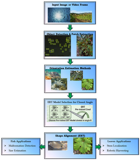
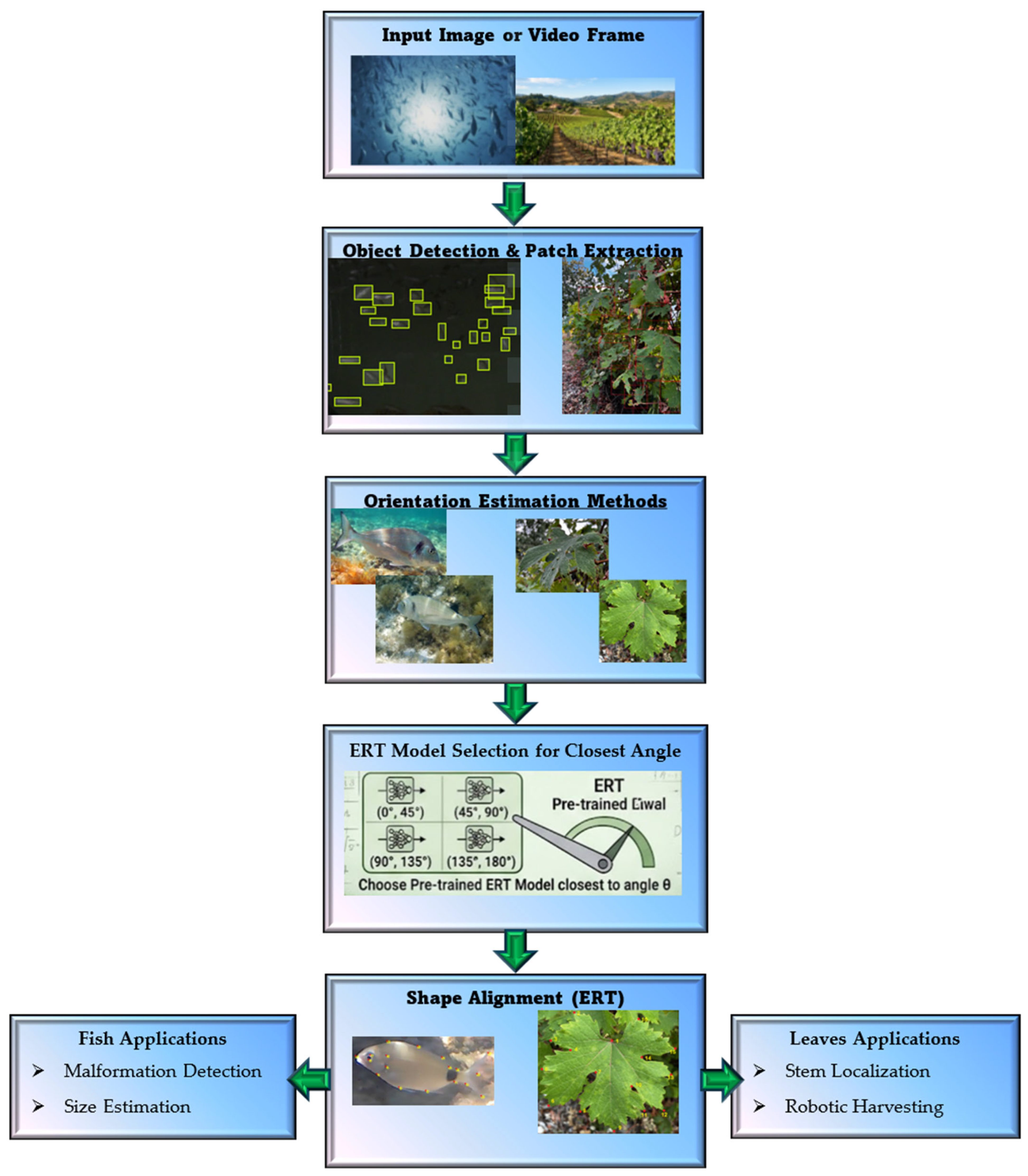
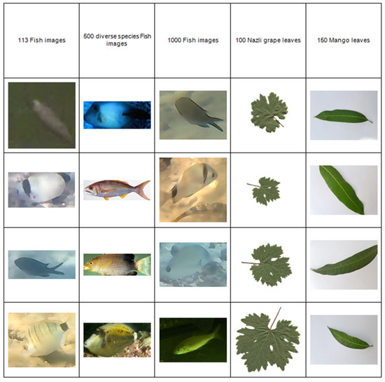
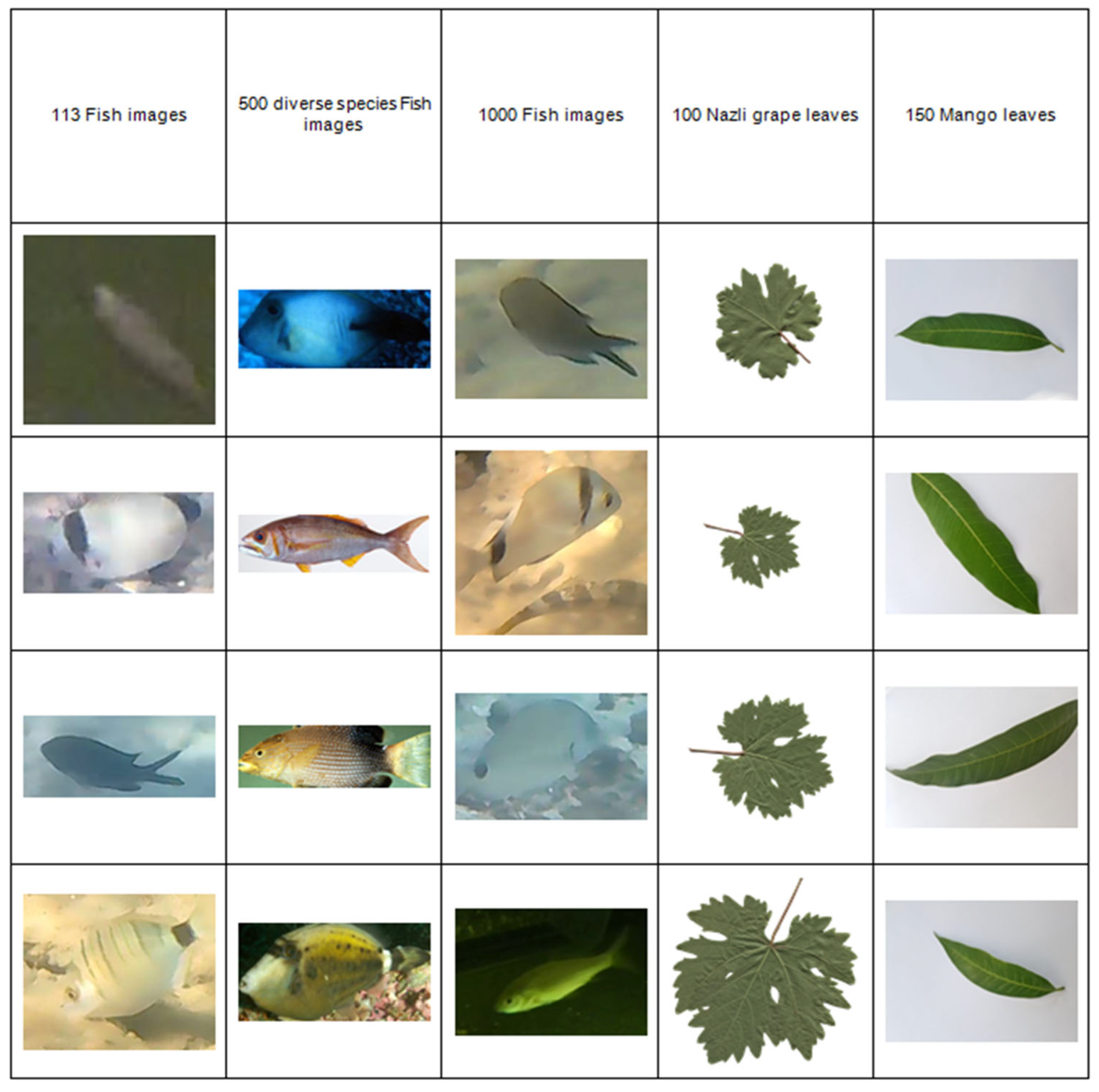
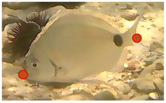
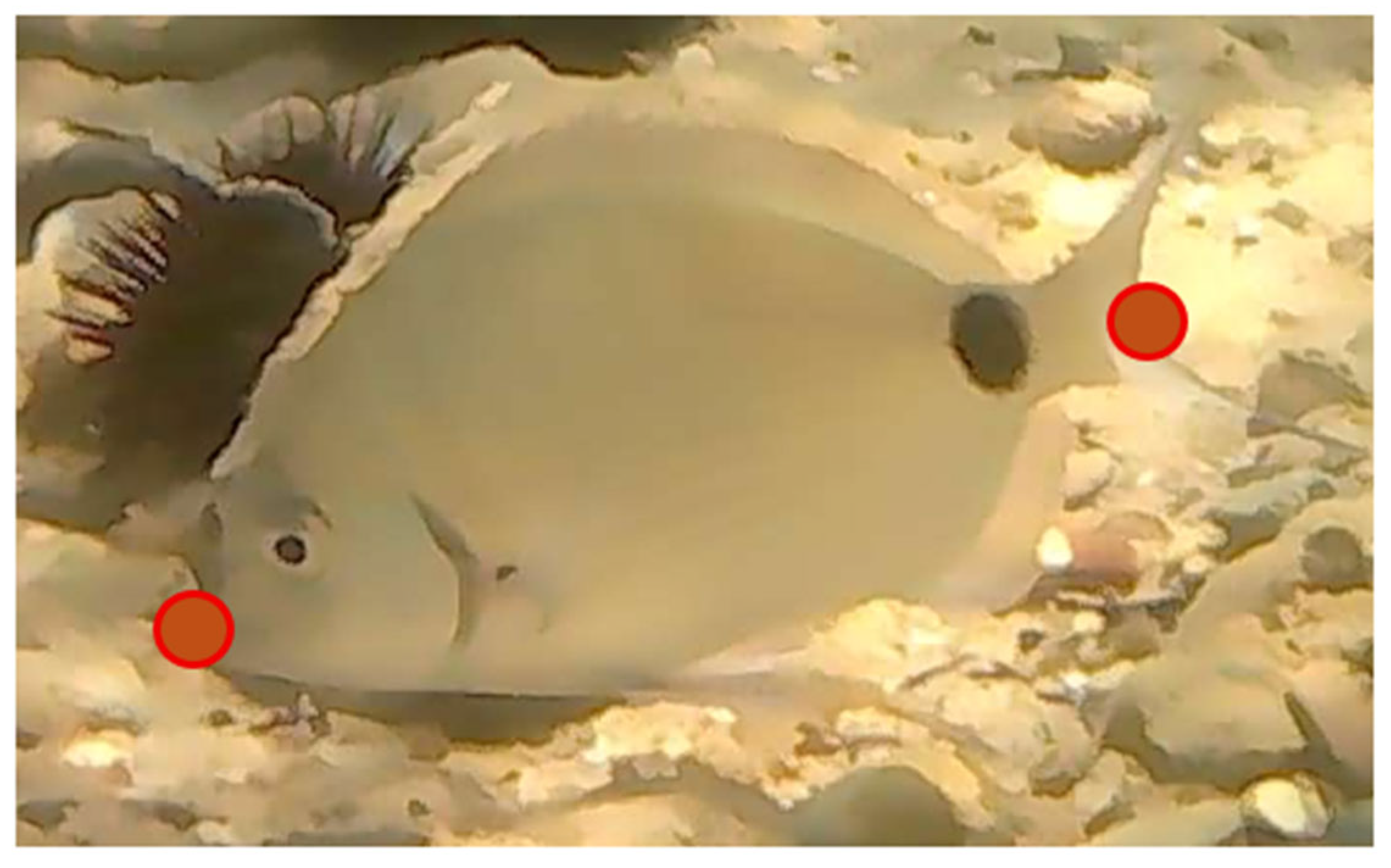
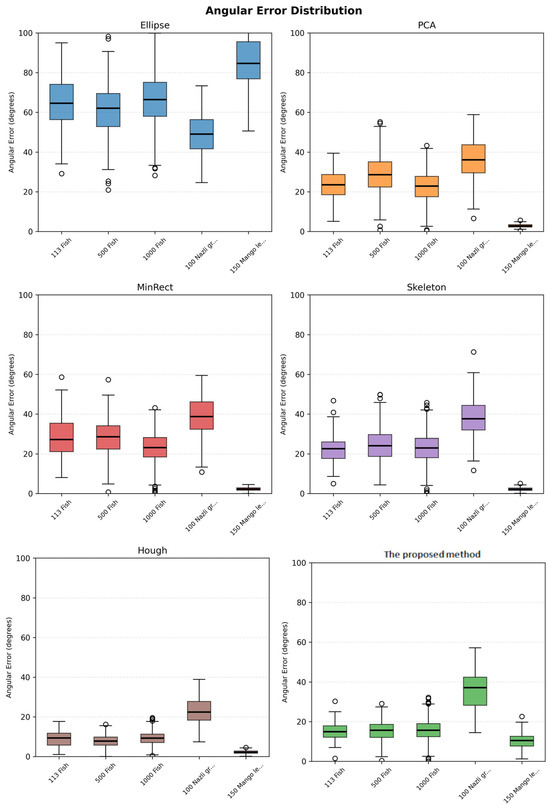
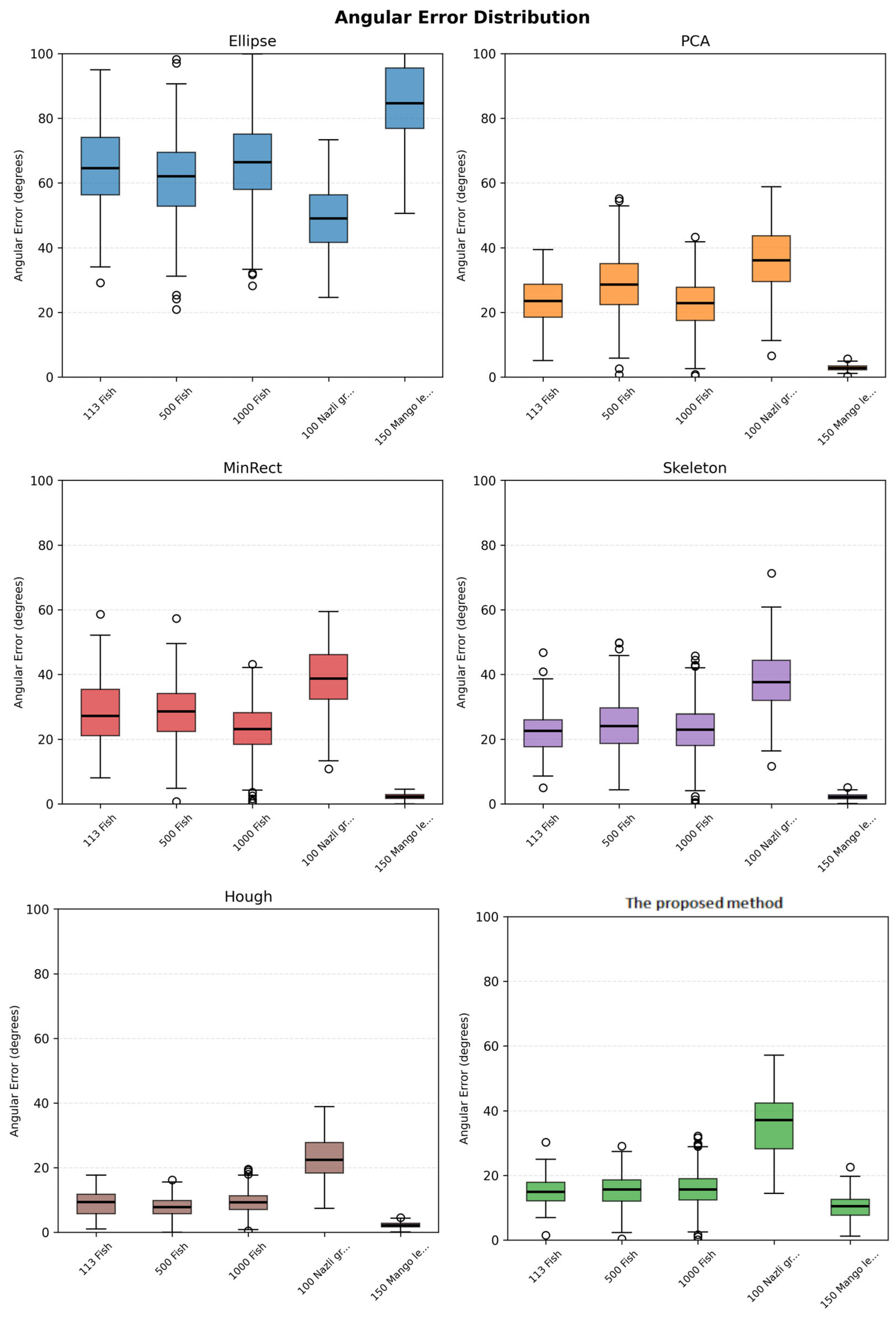
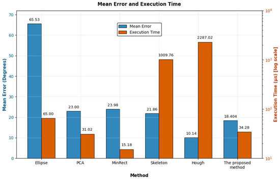

Disclaimer/Publisher’s Note: The statements, opinions and data contained in all publications are solely those of the individual author(s) and contributor(s) and not of MDPI and/or the editor(s). MDPI and/or the editor(s) disclaim responsibility for any injury to people or property resulting from any ideas, methods, instructions or products referred to in the content. |
© 2026 by the authors. Licensee MDPI, Basel, Switzerland. This article is an open access article distributed under the terms and conditions of the Creative Commons Attribution (CC BY) license.