


Abstract
Some passive wireless frequency-conversion approaches require an additional local oscillator or dual-frequency excitation, increasing circuit complexity. This paper proposes a single-frequency-excited wireless passive sensing mixer that exploits the nonlinear parasitic junction capacitance of a field-effect transistor (FET) coupled to a sensing resonator. By utilizing the voltage-dependent parasitic capacitance normally suppressed in conventional RF design, the circuit couples device nonlinearity with the characteristic response of the sensing resonant network to generate frequency-converted components separated from the incident carrier without an additional external local oscillator. First, the resonant response formed by the voltage-dependent FET gate–source (GS) capacitance and the front-end equivalent inductance is analyzed in terms of its operating-point-dependent natural frequency and nonlinear forced response. Under the modeling assumption that the internal sensing mode approximately modulates the front-end equivalent parameters periodically, a generalized forced Mathieu–Duffing model is used to describe the coupling among nonlinear restoring behavior, parametric modulation, and frequency conversion. A complete circuit is then simulated in ADS at 433 MHz. The input impedance and single-frequency spectrum are first characterized with the normal gate–drain parasitic capacitance Cdg. The Cdg branch is then set to zero while all surrounding circuit parameters and RF excitation conditions are kept unchanged; the normal Cdg model is subsequently restored for a separate optimization of the matching network. With only a 433 MHz RF excitation, the complete circuit produces non-harmonic frequency-conversion components near 420 and 446 MHz. These components remain observable when Cdg is set to zero, whereas the carrier response and input-impedance characteristics change. Matching optimization changes the input impedance at 433 MHz from 24.511 + j85.561 Ω to 49.529 + j2.150 Ω and increases the spectral response at the designated 420 and 446 MHz frequencies. Repeated measurements on fixed-parameter printed circuit board (PCB) configurations demonstrate repeatable converted-frequency output, and a separate wireless loading experiment shows a load-dependent received-frequency response. Over the 0–200 g loading range, the mean return-frequency shift reaches approximately 70.76 kHz. The simulations and measurements jointly support the feasibility of single-frequency-excited frequency conversion and wireless sensing readout, providing an approach to simplified, low-power wireless sensing systems.
1. Introduction
With the continued development of the Internet of Things (IoT), smart manufacturing, and ubiquitous sensing, the demand for long-term, low-maintenance data acquisition in complex environments has increased. Wireless passive sensors do not require built-in batteries or continuous active power supplies and therefore offer simple structures, low maintenance requirements, long service life, and convenient distributed deployment. They have been widely applied to industrial condition monitoring, environmental sensing, structural health monitoring, and biomedical detection [1,2].
Existing wireless passive sensing systems mainly encode and wirelessly read sensing information through resonance-frequency shifts, impedance modulation, and nonlinear frequency conversion. Inductor–capacitor (LC), surface acoustic wave (SAW), and radio-frequency identification (RFID) schemes typically map variations in the measurand to changes in resonant frequency, phase, or reflection coefficient [3,4,5]. However, when sensing perturbations are weak, wireless coupling distance increases, or the environment becomes complex, limited frequency shifts and echo variations are susceptible to propagation loss, background reflection, and system frequency instability.
To improve spectral distinguishability, passive frequency-conversion technologies exploiting device nonlinearities have attracted increasing attention [6,7]. Conventional mixers use two different excitation frequencies to generate sum- and difference-frequency products, while an ordinary nonlinear device driven by a single tone predominantly produces integer harmonics. This work examines a different operating mode: coupling a single external RF signal with an internal sensing-resonator response to produce frequency components separated from the carrier by non-integer multiples. Since the passive circuit has no independent power-gain stage, its response under weak excitation is particularly sensitive to device nonlinearity, resonant coupling, and impedance conditions.
Nonlinear dynamics offers a framework for analyzing this response. The Duffing model describes amplitude-dependent frequency responses caused by nonlinear restoring behavior, whereas the Mathieu model represents periodic variation of system parameters [8,9]. The charge–voltage relationship, conduction behavior, and parasitic capacitances of a radio-frequency field-effect transistor (FET) are intrinsically nonlinear and can participate in generating harmonics and combination-frequency components [10]. In particular, the voltage-dependent gate–source (GS) parasitic junction capacitance, together with the equivalent inductance of the input-matching network, contributes to the front-end resonant response. Variations in gate–source voltage or operating state alter the effective GS capacitance and local natural frequency, producing a nonlinear forced response with a variable natural frequency. When the internal sensing mode can be modeled as approximately periodic modulation of the front-end equivalent parameters, a generalized forced Mathieu–Duffing equation provides a description of nonlinear restoring behavior, periodic parameter modulation, and RF forcing. Instead of suppressing parasitic-capacitance nonlinearity as an unwanted RF imperfection, the proposed design makes use of its voltage dependence, particularly under specified forward electric-field conditions, and combines it with the sensing resonator for single-frequency nonlinear frequency conversion.
On this basis, a wireless passive mixer is designed using FET parasitic junction-capacitance nonlinearity and a forced response with a variable local natural frequency. The system comprises a shared transmit/receive antenna, an input-impedance matching network, an FET nonlinear mixing element, a gate sensing resonator, a drain frequency-selective load network, and a microvoltage adjustment branch. The single-frequency RF signal is coupled to the FET through the matching network, where the GS parasitic junction capacitance and the equivalent front-end inductance jointly establish local resonance conditions. The nonlinear forced response couples with the internal sensing resonator to generate combination-frequency components under suitable parameter conditions. Variations in the sensing parameters affect the internal resonant response and mixed-component frequencies, while the drain network regulates input impedance and spectral-energy distribution. The objective is to relate device nonlinearity, sensing-resonance coupling, and single-frequency mixing to a practical low-power wireless sensing circuit.
The main contributions of this work are as follows.
- (1)
- A wireless passive nonlinear mixer operating under a single externally applied RF frequency is proposed. Coupling the FET nonlinear unit with the internal sensing resonant network produces non-harmonic combination-frequency components without a second external mixing excitation. Sensing information is represented by changes in the frequencies of the mixed components, enabling frequency encoding and wireless readout.
- (2)
- A nonlinear-dynamics analysis that deliberately exploits FET parasitic GS junction-capacitance nonlinearity is developed. The GS capacitance–voltage (C–V) relation characterizes voltage dependence, and the corresponding junction charge–voltage (Q–V) relation provides the nonlinear restoring terms. The resonant response formed by the GS junction capacitance and the front-end equivalent inductance is represented as a forced system with an operating-point-dependent natural frequency. When the internal sensing mode can be approximated by a periodic response, an equivalent periodic-parameter term is included to establish a generalized forced Mathieu–Duffing model for analyzing the relationship between parasitic-capacitance nonlinearity and the observed mixing response.
- (3)
- An analysis framework is established for nonlinear mixing and frequency conversion under single-frequency excitation. It considers the voltage dependence of the GS parasitic junction capacitance, transistor conduction nonlinearity, sensing-resonator coupling, and the frequency selectivity of the surrounding network, including the effects of the drain load on input impedance and spectral distribution. With the original, non-optimized matching network and normal Cdg as a common baseline, separate controls are performed by zeroing Cdg and by optimizing the surrounding matching network. These comparisons assess the effects of the GD parasitic branch and matching conditions on the input impedance and spectral response within the same circuit topology.
- (4)
- The circuit is evaluated through Advanced Design System (ADS) simulations, printed circuit board (PCB) measurements, and wireless pressure-sensing tests. Under a single 433 MHz RF excitation, the complete circuit produces non-harmonic components approximately ±13 MHz from the carrier. Seven same-board measurements are carried out for each of two fixed circuit configurations, repeatedly observing converted-frequency outputs at recorded 433 MHz excitation levels of approximately 1.91–2.51 μW. In an independent wireless test with a single 433 MHz excitation, a load-dependent received component is detected near 421.5 MHz, with a mean shift of approximately 70.76 kHz over the 0–200 g loading range.
The remainder of this paper is organized as follows. Section 2 reviews the relevant technologies and research progress; Section 3 presents the circuit architecture and theoretical model; Section 4 reports circuit simulations; Section 5 presents PCB measurements and wireless sensing validation; and Section 6 summarizes the findings and future work.
2. Research Progress in Wireless Passive Sensing and Nonlinear Frequency-Conversion Technologies
2.1. Resonance-Frequency-Shift-Based Wireless Passive Sensing
Resonance-frequency-shift-based wireless passive sensing uses external physical quantities such as temperature, pressure, humidity, and strain to alter the equivalent inductance, capacitance, or propagation parameters of a sensing structure. These changes cause shifts in resonant frequency, phase, or reflection characteristics that can be detected wirelessly by an external reader. Because continuous active power is not required, such systems offer simple structures, low maintenance requirements, and suitability for long-term deployment.
LC resonant sensors are a representative form of wireless passive sensing and operate by converting changes in sensitive-element parameters into shifts of the resonant frequency. Ong et al. demonstrated the feasibility of wireless passive resonant circuits for temperature, humidity, pressure, and dielectric-property sensing [3]. The resonant frequency of an ideal LC resonant network can be expressed as follows:
where f0 is the resonant frequency, and L and C are the equivalent inductance and capacitance, respectively. When an external physical quantity causes L or C to change, the sensing information can be read from the shift of f0. With advances in flexible electronics and microfabrication, LC passive sensors have increasingly moved toward flexible and wearable implementations. For example, Sun et al. developed a flexible wireless passive LC pressure sensor that enabled wireless detection of pressure variations [11].
SAW sensors use the sensitivity of surface-acoustic-wave velocity, phase, or resonant frequency in piezoelectric materials to environmental parameters. These devices offer relatively high quality factors and good frequency stability and have been used for temperature, pressure, strain, and biochemical sensing. More recently, piezoelectric materials such as AlN and ScAlN have improved the temperature response and environmental adaptability of SAW devices; however, fabrication generally relies on piezoelectric films, interdigital transducers, and micro/nanofabrication processes, which impose constraints on cost and manufacturing complexity.
In addition to resonant structures, RFID-based passive sensing commonly changes the antenna reflection coefficient through load-impedance modulation and thereby encodes sensing information into the backscattered signal. Nikitin and Rao showed that the readout performance of passive ultra-high-frequency (UHF) RFID systems is jointly limited by the tag activation threshold, antenna gain, propagation loss, and the backscatter link [12]. The excitation frequency, coupling condition, and readout method of wireless passive resonators also directly affect the distinguishability of their resonant features [13].
Overall, LC, SAW, and RFID techniques provide mature passive sensing approaches, using changes in resonance, phase, or reflection to represent sensing information. When perturbations and wireless coupling are weak, quality factor, propagation loss, and interference can constrain these responses. Mapping sensing information into combination-frequency components separated from the incident carrier offers another means of improving spectral distinguishability and motivates the study of non-harmonic mixing with single-frequency RF excitation.
2.2. Passive Wireless Mixing and Frequency-Conversion Techniques
Passive wireless mixing and frequency-conversion techniques exploit the current–voltage, charge–voltage, or switching nonlinearities of diodes and other nonlinear devices to couple signals at different frequencies and generate sum-frequency, difference-frequency, harmonic, and intermodulation components. Compared with conventional sensing methods based on small resonance-frequency shifts, frequency translation can move sensing information away from the carrier and thereby reduce interference from strong carrier leakage and co-frequency background reflections.
Conventional passive RF mixers commonly use diode nonlinearity for frequency conversion. Let the input voltage applied to the nonlinear device be v(t); around an operating point, the device current can be expressed as follows:
i(t) = a1v(t) + a2v2(t) + a3v3(t)+…
When the input contains multiple components at frequencies f1 and f2, the higher-order nonlinear terms generate components satisfying:
fm,n = |mf1 ± nf2|, m,n = 0,1,2,…
Maas showed that the conversion performance of passive diode mixers depends jointly on device nonlinearity, impedance matching, and RF drive level [14]. Because a passive circuit has no independent power-gain stage, its mixed-frequency components are generally weak under low RF drive. With RF integrated-circuit development, complementary metal–oxide–semiconductor (CMOS) passive mixers based on periodic switching of metal–oxide–semiconductor (MOS) transistors have been studied extensively. Such circuits offer low static power consumption and high integration density but generally exhibit conversion loss and are affected by on-resistance, parasitic capacitance, and nonideal switch drive [15].
In wireless passive sensing, intermodulation communication and harmonic backscatter extend the use of nonlinear frequency conversion. Viikari et al. reviewed passive wireless sensors using intermodulation communication, where multiple external excitation frequencies generate intermodulation products in a passive node and encode sensing information onto those components [6]. Harmonic RFID systems studied by Mondal et al. convert incident RF signals into second or higher harmonics to mitigate fundamental-carrier leakage and part of the background scattering [7]. These results demonstrate the feasibility of passive frequency conversion, although their frequency-generation mechanisms principally involve multi-tone intermodulation or integer harmonics. In comparison, nonlinear coupling between a single external RF excitation and an internal sensing resonator offers another means of producing mixed-frequency components not related to the carrier by a simple integer ratio. This response depends on internal circuit dynamics and cannot be equated with ordinary harmonic generation in a static nonlinearity.
In addition to explicit diode and switching nonlinearities, parasitic parameters within transistors are voltage-dependent. Niemeier et al. identified nonlinear parasitic capacitances in OFF-state MOS transistors as an important source of RF harmonics [16]. Previous work has also demonstrated the use of FETs in zero-power or passive intermodulation sensing systems [17]. However, conventional RF design usually suppresses or compensates for parasitic-capacitance nonlinearity. Deliberately exploiting the voltage dependence of the FET GS parasitic junction capacitance, particularly under specified forward-field conditions, may allow this nonlinearity to influence the front-end dynamic parameters and sensing-resonance coupling, providing another direction for improving low-power nonlinear frequency conversion.
To provide an overview of representative passive nonlinear frequency-conversion and wireless sensing approaches, Table 1 summarizes their operating frequencies, excitation schemes, reported RF power levels, converted-frequency outputs, and validation conditions. The reported power values are presented according to the definitions and test conditions used in the corresponding studies.
Table 1.
Comparison of operating conditions and reported frequency-conversion results in representative passive wireless sensing studies.
The reported RF power values are based on the measurement conditions and reference planes specified in the respective studies, including simulation excitation, wired input power, signal-generator output, and activation or onset thresholds. These quantities differ from the RF power delivered to or received by a sensing device. The values are retained in their original reporting forms and are used to compare operating conditions and implementation approaches rather than directly rank conversion performance or power efficiency.
Table 1 summarizes representative passive frequency-conversion approaches, including dual-tone intermodulation, harmonic conversion, and single-frequency excitation involving internal oscillation or parametric coupling. These studies differ in operating frequency, excitation method, experimental configuration, and RF power definition. Accordingly, the reported power levels and converted-signal characteristics are interpreted within their respective measurement conditions rather than compared as directly equivalent performance metrics. The proposed circuit utilizes the coupling between voltage-dependent FET GS parasitic capacitance and an internal sensing resonator to realize frequency conversion under a single external RF excitation. Repeated PCB measurements demonstrate observable converted-frequency components at low recorded excitation levels, while separate wireless loading experiments confirm load-dependent frequency readout. The comparison therefore highlights differences in frequency-conversion mechanisms, excitation requirements, and experimental validation approaches.
In summary, diode mixers, CMOS passive mixers, intermodulation communication, and harmonic backscatter provide a foundation for passive frequency conversion. Nevertheless, further investigation is warranted into the coupling between an internal sensing-resonance response and transistor parasitic junction-capacitance nonlinearity under a single external excitation. Establishing a physical link among voltage-dependent GS capacitance, the variable local natural frequency, nonlinear sidebands, and load selectivity is a particular focus of this work.
2.3. Nonlinear Dynamics in RF Devices
As device dimensions shrink, operating frequencies rise, and signal amplitudes increase, nonlinear charge–voltage relations, parasitic capacitances, and conduction characteristics in RF devices can significantly affect system dynamics and may produce amplitude-dependent frequency shifts, harmonics, intermodulation, and multistability. Nonlinear dynamics provides a unified framework for describing these responses in terms of restoring forces, damping, and external excitation.
The Duffing oscillator is a classical model for nonlinear forced response and can be written as follows:
Here, β represents the cubic nonlinear restoring coefficient. The Duffing model characterizes resonance-curve bending and amplitude-dependent frequency shifts, as well as jumps, hysteresis, or multistability under suitable excitation and damping conditions. It describes state-dependent nonlinear restoration; periodic variations in system parameters can be represented separately by a Mathieu-type model.
The Mathieu model is mainly used to describe periodic parametric modulation and can be written in its basic form as follows:
Here, h and ωm denote the depth and angular frequency of parametric modulation, respectively. Unlike ordinary external forcing, Mathieu-type excitation changes the effective restoring coefficient periodically. In the RF circuit model, the Mathieu parameter term thus represents periodic equivalent-parameter changes induced by the internal mode, as distinct from the nonlinear restoring response associated with voltage dependence alone.
When periodic parameter modulation, nonlinear restoring forces, and external forcing occur together, a generalized forced Mathieu–Duffing model may be adopted:
Here, α and β are the quadratic and cubic nonlinear restoring coefficients, ωs denotes the modulation angular frequency, and ωRF is the external RF excitation angular frequency. Unlike the Duffing-only or Mathieu-only models, this formulation incorporates nonlinear restoration, periodic parameter variation, and forced response in a common framework for examining their coupled influence on frequency response. Lyu et al. combined Duffing nonlinearity and mode localization to enhance the sensitivity of a microelectromechanical-system (MEMS) mass sensor [23], whereas Wang et al. employed a Mathieu–Duffing oscillator for weak periodic-signal detection, demonstrating the analytical value of coupled parameter modulation and nonlinear response [24].
These concepts can also be applied to nonlinear RF semiconductor circuits. The present study exploits the voltage dependence of the FET parasitic GS junction capacitance, with particular attention to its nonlinear variation under specified forward electric-field conditions. The capacitance and surrounding matching network are mapped to effective restoring, damping, and local natural-frequency characteristics. Under the modeling assumption that the internal sensing mode can be approximated by a periodic response, an equivalent periodic parameter term describes its coupling to the front-end restoring coefficient. The generalized forced Mathieu–Duffing framework is then used to examine single-frequency RF forcing, sensing-resonator coupling, and nonlinear frequency conversion.
2.4. Summary of Research Gaps
Wireless passive sensing has developed a substantial foundation in resonant-frequency shifts, impedance modulation, intermodulation communication, harmonic backscatter, and nonlinear resonators. LC, SAW, and RFID techniques provide passive sensing and wireless readout, while nonlinear devices such as diodes and MOS transistors generate harmonics, intermodulation, and combination-frequency components. Three aspects remain especially relevant to the present investigation: non-harmonic conversion under single-frequency excitation, deliberate utilization of junction-capacitance nonlinearity, and a physical connection between device-level characteristics and system-level nonlinear dynamics.
(1) Non-harmonic frequency conversion and sensing encoding under single-frequency excitation. Whereas conventional mixing commonly uses two tones to produce sum- and difference-frequency components, this study examines nonlinear coupling between one external RF tone and an internal sensing-resonator response, with particular emphasis on non-integer-related components and frequency-domain sensing readout.
(2) Deliberate utilization of parasitic junction-capacitance nonlinearity. Conventional RF design often suppresses or compensates for parasitic capacitance to preserve matching and linearity. Here, the FET GS parasitic junction capacitance is used as a voltage-dependent parameter, with its effects on front-end impedance, local natural frequency, and low-power forced response investigated under relevant operating and forward-field conditions.
(3) Physical linkage between device-level nonlinearity and system-level mixing dynamics. Conventional passive-mixer studies frequently emphasize nonlinear transfer functions and spectra, while Duffing and Mathieu descriptions employ effective nonlinear coefficients. For FET-junction-capacitance-based mixing circuits, the capacitance–voltage (C–V) characteristic used for device characterization must be distinguished from the charge–voltage (Q–V) relation used in the dynamical model. This distinction helps connect variable natural frequency, sensing-resonance coupling, and mixed-frequency components while identifying the different physical sources of ordinary nonlinear restoration and periodic parameter modulation.
To address these issues, this work presents a wireless passive mixer based on FET parasitic GS junction-capacitance nonlinearity and a forced response with a variable local natural frequency. By exploiting the voltage dependence of the parasitic capacitance together with input matching, the gate sensing resonator, and the frequency-selective drain load, the circuit realizes non-harmonic conversion under a single external RF excitation. Under the modeling assumption that the internal sensing mode can be approximated by a periodic response, a generalized forced Mathieu–Duffing model is used to describe the parametric coupling between nonlinear restoration and the sensing mode, connecting device-level capacitance nonlinearity with effective system dynamics.
This work aims to provide a unified analysis framework for single-frequency excitation, nonlinear parasitic-capacitance response, and sensing-resonance coupling, and to analyze the effects of frequency conversion and load regulation on sensing readout. ADS simulations, PCB measurements, and wireless pressure-sensing experiments are used to verify low-power mixing and load-dependent frequency response.
3. Circuit Design and Theoretical Modeling
This section establishes an equivalent model of the wireless passive mixer circuit based on the system architecture and device physics. The modeling objective is to project the interactions among input matching, GS junction capacitance, sensing resonance, nonlinear frequency conversion, and the D-terminal load onto a small set of state variables with clear physical meaning, thereby providing a unified basis for subsequent device-level, circuit-level, and spectral validation.
3.1. Overall Circuit Architecture and Signal Transmission
The proposed system consists of a transmit/receive antenna, an impedance-matching circuit, an FET nonlinear mixing unit, a sensing circuit, a D-terminal resonant load, and a microvoltage branch, as shown in Figure 1. The shared antenna is a single-port device that receives RF excitation and returns the mixed signal. The matching circuit is formed by a passive inductive network and transforms the antenna-port impedance to the RF input impedance of the FET. The sensing circuit converts an external physical quantity into a change in resonant parameters. The FET exploits the nonlinear junction-capacitance and channel current–voltage characteristics to provide frequency coupling, while the D-terminal network regulates the transmission paths of different frequency components through a frequency-selective impedance boundary.
Figure 1.
Overall architecture of the wireless passive mixing system.
A specific implementation of the circuit is shown in Figure 2. L1, L2, and L3 form the T-type matching network; the sensing inductor Ls and sensitive capacitor Csense form the G-terminal sensing resonant branch; and Lp and Cp form the D-terminal parallel resonant network. The microvoltage branch is used to adjust the static gate-source operating point of the FET. Zero bias is the basic operating mode of the system. When a microbias is introduced, the main RF signal path remains passive, and the microbias is used only to shift the device operating point.
Figure 2.
Specific circuit configuration of the wireless passive mixing system. V denotes the microbias voltage, and the arrow across Csense indicates a variable sensing capacitance.
Let the antenna-port reference impedance be Z0 and the equivalent input impedance observed from the antenna be Zin. The input reflection coefficient can then be written as follows:
The matching network increases the RF voltage coupled to the nonlinear branch near the main operating frequency; the final magnitude of the target converted component is jointly determined by matching, FET nonlinear conversion, and the frequency selectivity of the drain network.
Let the incident antenna voltage be Vinc and the complex transfer function from the matching network to the GS terminal be Hin(ω). The equivalent forcing amplitude acting on the front-end principal mode is then:
Ve(ωc) = |Hin(ωc)|Vinc
When the input network and the GS equivalent branch are close to series resonance and the loss is small, the GS-terminal voltage can exhibit a resonance-induced increase analogous to a quality-factor enhancement. This increase results from passive energy storage and does not represent positive power gain generated by the circuit.
3.2. Nonlinear FET GS Junction-Capacitance Model
The FET GS junction exhibits voltage-dependent capacitance characterized by a nonlinear relation between junction charge Qgs and gate–source voltage Vgs. The corresponding local differential capacitance is defined as follows:
The C–V characteristic describes the junction capacitance as a function of gate–source bias; its ordinate is capacitance, not junction charge. In Equation (9), Qgs is a theoretical modeling variable, and its increment relative to the reference operating point follows by integrating Cgs(Vgs). The measured or simulated capacitance characteristic is therefore distinct from the incremental-charge coordinate used in the dynamical derivation.
Consider the static operating point V0 set by the microbias VB. Let q = Qgs − Qgs(V0) denote the charge relative to the static charge and v = Vgs − V0 the AC increment. To map the device parameters directly to the dynamic restoring terms, the inverse charge–voltage function is expanded around the operating point as:
v(q) = a1q + a2q2 + a3q3 + O(q4)
Let C0 = Cgs(V0), and let C1 and C2 denote the first and second voltage derivatives, respectively, of Cgs evaluated at V0. The coefficients of the inverse function are then:
Here, a1 determines the small-signal restoring stiffness near the operating point, a2 represents the quadratic nonlinearity arising from device asymmetry, and a3 represents the cubic nonlinearity. The sign of a3 determines whether the equivalent Duffing response tends toward hardening or softening. The quadratic term a2 also produces static offsets, even-order harmonics, and conventional sum- and difference-frequency components, and therefore cannot be neglected a priori in the FET mixing model. Changes in microbias alter C0, C1, C2, and the corresponding nonlinear coefficients.
The first- and second-order voltage derivatives of the capacitance describe the local variation of the C–V characteristic. During parameter extraction, these derivatives should be obtained from capacitance data at multiple bias points or a validated voltage-dependent device model.
Taking the incremental charge q of the nonlinear GS-capacitance branch as the generalized coordinate, let Le denote the equivalent inductance formed by the input-matching network, interconnect parasitics, and principal-mode projection, and let Re denote the equivalent series loss incorporating conductor loss, device loss, and radiative coupling. The front-end principal-mode equation can then be written as:
Through the junction capacitance–voltage (C–V) characteristic and the associated junction charge–voltage (Q–V) relation, the front-end principal-mode equation links device-level nonlinearity with the forced circuit response. Variations in GS capacitance jointly affect the local natural frequency, nonlinear restoring coefficients, FET port impedance, and coupling to the surrounding network, giving rise to coupled changes in impedance and spectrum.
The microbias and resonant voltage jointly determine whether the channel enters the pronounced nonlinear conduction-transition region. Let the GS-terminal fundamental amplitude be Ag. A convenient approximate condition for crossing both sides of the threshold within one RF cycle is:
where Vth is the equivalent conduction threshold and VD is the barrier-voltage upper limit allowed by the junction-capacitance model. If Ag is expressed as a peak voltage and Hg denotes the transfer coefficient from antenna-port power to GS fundamental voltage, the input power required to first approach the threshold can be estimated as:
The above expression indicates that the excitation threshold can be reduced by increasing input coupling and resonant voltage or by appropriately shifting the static operating point.
3.3. Sensing Network and Time-Varying Natural-Frequency Model
The sensing branch converts the measurand X into a change in the equivalent inductance Ls(X) or equivalent capacitance Cs(X). When loss is small and a single resonant mode dominates, its characteristic angular frequency is:
A first-order linearization around the operating point gives the relative variation of the sensing frequency:
To discuss the physical origin of the Mathieu parameter term, a normalized sensing mode y is introduced. Its lower-order dynamics can be described as follows:
In Equation (17), Fs(t) denotes the effective coupling excitation generated by the front-end response through the gate resonant network and device nonlinearity. The sensing mode changes the front-end restoring coefficient through the G-terminal voltage, GS junction capacitance, or equivalent input impedance. With a front-end linear restoring coefficient a1(t) = a1 + κy(t), the dominant-mode approximation represents the periodic sensing response as follows:
y(t) = Ascos(ωst + φs)
Under the weak-modulation approximation, the instantaneous front-end natural angular frequency can be expressed as:
Here, ω0 is the local natural angular frequency near the operating point, and h is the dimensionless parameter-modulation depth.
3.4. Generalized Forced Mathieu–Duffing Model
In the equivalent model, a periodic parameter term represents modulation of the front-end restoring coefficient by the sensing mode. This term and the quadratic and cubic nonlinear restoring terms derived from the voltage dependence of GS junction capacitance are incorporated into the front-end principal-mode equation. Dividing by the equivalent inductance Le yields the generalized forced Mathieu–Duffing model used in this work:
The main physical meanings of the variables and parameters are summarized in Table 2.
Table 2.
Main parameters of the Mathieu–Duffing model and their circuit interpretation.
Equation (20) incorporates external RF excitation, GS junction-capacitance nonlinearity, and sensing-mode coupling into a unified dynamical description. Table 2 lists the physical meanings and circuit origins of the parameters. On this basis, the subsequent simulations analyze the effects of device characteristics, input matching, and load networks on the mixing response. Experiments further verify frequency-converted output and wireless readout of sensing information under single-frequency excitation, linking circuit structure, nonlinear response, and sensing applications.
3.5. Nonlinear Mixing and Frequency-Selective Return Transmission
For a steady response synchronized with single-frequency excitation, the spectral components consist of the fundamental and its integer harmonics. Mixing, by contrast, involves coupling different frequency components through a nonlinear device. Only one external RF excitation is applied here; the carrier response and the internal sensing-branch dynamics are analyzed as a coupled system to explain non-harmonic mixing. Equation (20) describes nonlinear restoration and sensing-mode parameter coupling; the following discussion uses the FET nonlinear transfer characteristics and surrounding frequency-selective network to explain combination-frequency generation and return transmission.
To analyze frequency coupling between the carrier and internal dynamics, the equivalent GS terminal voltage is represented by a carrier component and a component at the characteristic sensing frequency:
vgs(t) = Vccos(ωct) + Vscos(ωst)
The FET drain current, or equivalent output current, is expanded around the operating point as follows:
Substituting Equation (21) into Equation (22), the cross product of the quadratic term generates sum- and difference-frequency components at ωc + ωs and ωc − ωs. Cubic and higher-order terms additionally generate harmonics, frequency multiplication, and higher-order combinations of the form mωc + nωs. This relation shows that nonlinear coupling of the carrier and the internal response can represent sensing information at combination frequencies without a second external RF input. Upper- and lower-sideband amplitudes are jointly affected by the front-end response and the selectivity of the surrounding network and need not be equal.
The D-terminal Lp–Cp network forms a parallel-resonant boundary near the target frequency. Including a finite loss resistance RD, its equivalent impedance is:
The FET GD and DS parasitic branches form multiport coupling between the drain termination and the input port. Using Z parameters for the locally linearized two-port network, the input impedance with the D-terminal load is:
Equation (24) indicates that the D-terminal load changes the input impedance through internal device coupling and also affects transmission of mixing components from inside the FET to the antenna. Let Ak,int denote the mixing component generated inside the device at the target frequency, and let Hret denote the corresponding return-transfer function. The antenna-port output power can then be expressed as:
Equation (25) indicates that the measured mixing output depends jointly on nonlinear frequency conversion inside the device and return-transmission capability at the target frequency. Sensing information is represented by the frequency of the target mixing component. Changes in the measurand alter the equivalent inductance or capacitance of the sensing branch and consequently its resonant characteristics. In the frequency-coupling description above, changes in the characteristic sensing frequency are reflected in the target mixing frequency through nonlinear coupling with the carrier. Internal resonant response and nonlinear frequency conversion thus map changes in sensing parameters to frequency changes in the wireless return signal, enabling wireless readout of sensing information.
In summary, this section links input matching, nonlinear GS junction capacitance, sensing-resonance coupling, and return transmission through the D-terminal load. The generalized forced Mathieu–Duffing model describes nonlinear restoration and sensing-mode parameter coupling; FET nonlinear expansion establishes combination-frequency relations; and frequency-selective networks link internal mixing to antenna-port output, offering an overall explanation of frequency-converted output and sensing readout under one external excitation.
4. Circuit Simulation
To investigate the proposed wireless passive nonlinear mixer, a unified complete-circuit model is established in ADS to analyze the basic device characteristics, original input matching, nonlinear mixing with normal Cdg under single-frequency excitation, the Cdg-zeroing control, and optimization of the surrounding matching network.
The simulation sequence begins with the FET DC transfer characteristic, equivalent GS capacitance, and parasitic-branch frequency responses. The S-parameter, transient, and spectral responses are then obtained for the original, non-optimized matching network with normal Cdg, providing a common baseline. With all surrounding matching parameters unchanged, only Cdg is set to zero to evaluate changes in impedance and spectrum. Finally, the normal Cdg model is restored, and the matching-network parameters are optimized. Thus, the Cdg-branch and matching-network effects are examined in two separate controlled comparisons.
This chapter proceeds from device characterization to original input impedance, the complete-circuit single-frequency mixing spectrum, the Cdg-zeroing control, and matching optimization. DC characteristics, equivalent capacitances, S-parameters, transient waveforms, and fixed-frequency spectral markers are used to compare the response of the same circuit topology under controlled conditions.
4.1. Simulation Environment and Parameter Settings
ADS is used as the main RF simulation platform, together with S-parameter, transient, spectral, and Momentum electromagnetic analyses. S-parameters provide input reflection, impedance, and Smith charts; transient and spectral analyses characterize the dynamic response and components near the carrier; Momentum is used to analyze the electromagnetic characteristics of the PCB structure.
The complete circuit is operated around 433 MHz using a single external RF excitation and a 50 Ω port reference impedance. The commercial ATF54143 FET is used as the representative nonlinear device, modeled with its conduction and parasitic characteristics. The modeling approach also provides a basis for extending the analysis to other MOS/FET devices with voltage-dependent parasitic capacitance.
Separate DC and GS/GD/DS parasitic-branch models are first used to characterize FET conduction, equivalent GS capacitance, and frequency response. The normal-Cdg circuit with the original, non-optimized matching network is adopted as the common baseline: Section 4.3 presents its input reflection and impedance, and Section 4.4 presents its transient response and spectrum under a single 433 MHz excitation. In Section 4.5, only the FET gate–drain parasitic capacitance Cdg is set to zero, while the surrounding circuit, 433 MHz excitation, RF port, and spectral-extraction conditions remain unchanged. In Section 4.6, normal Cdg is restored, and only the surrounding matching-network parameters are optimized.
All three controlled circuit states use port 2 as the RF excitation port, with S22 describing input reflection over a 0–1 GHz sweep. Transient waveforms are displayed over 0–500 ns, and the spectrum is obtained from the same ADS node voltage TRAN.Vin using fs(TRAN.Vin), focusing on the 433 MHz carrier and adjacent converted-frequency components. The Cdg-zeroing comparison and matching-optimization comparison are discussed separately. Table 3 summarizes the simulation settings.
Table 3.
Main circuit-simulation settings.
Three controlled states of the complete circuit are considered. State A is the baseline with the original, non-optimized matching network and normal Cdg. In state B, only Cdg is set to zero while the original matching parameters remain unchanged. State C retains the normal-Cdg model and uses an optimized surrounding matching network. The A–B comparison evaluates the effects of the Cdg branch on input impedance and spectral response, whereas the A–C comparison evaluates matching optimization. Setting Cdg to zero changes both the capacitance magnitude and coupling conditions and does not selectively remove junction-capacitance nonlinearity. Spectral MARK values are extracted from simulated node voltages and do not directly represent antenna-radiated power or conversion gain.
4.2. Basic FET Characterization
Device-level FET characterization is first performed to obtain parameters required for subsequent input-matching, junction-capacitance, and nonlinear-mixing analyses. The DC transfer characteristic, GS equivalent capacitance, and the frequency responses of the GS, GD, and DS parasitic branches are examined to provide a parameter basis for the complete-circuit analysis.
4.2.1. DC Transfer Characteristic
A gate-source voltage sweep is first performed to obtain the drain-current dependence on gate-source voltage. The DC transfer characteristic can be expressed as:
ID = f(VGS,VDS)
The simulated transfer characteristic is shown in Figure 3. At low VGS, the drain current is close to zero, and the device is in cutoff; as VGS increases, the drain current rises nonlinearly.
Figure 3.
DC transfer characteristic of FET drain current versus gate-source voltage.
The DC sweep of the current FET model shows a transition from cutoff and weak conduction to pronounced conduction over approximately 0.35–0.52 V, providing an operating-state reference for discussing nonlinear conduction.
4.2.2. GS Equivalent Capacitance and Package Parasitics
The GS-branch equivalent capacitance is further extracted under zero-bias conditions. Because the GS branch is predominantly capacitive near 433 MHz, the equivalent capacitance can be estimated from the imaginary part of the input impedance:
Figure 4 presents the equivalent capacitance-frequency (C-f) characteristics of the bare chip and the packaged model GS under a fixed zero bias condition. Near 433 MHz, the effective capacitance is approximately 2.0 pF for the bare die and 2.4 pF when package parasitics are included.
Figure 4.
Equivalent GS capacitance–frequency (C–f) characteristics of bare-die and packaged models at fixed zero bias.
The capacitance values in Figure 4 are calculated from ADS frequency-domain impedance at zero bias and characterize the effective RF capacitance of the GS branch near 433 MHz. They represent a capacitance–frequency (C–f) sweep rather than a capacitance–voltage (C–V) scan; voltage derivatives of the junction capacitance require bias-dependent data. Package leads, pads, and interconnections are considered through their contribution to the complete circuit response.
4.2.3. Frequency Responses of the GS, GD, and DS Parasitic Branches
To examine the influence of individual parasitic paths on the RF response, zero-bias S-parameter sweeps are performed for the GS, GD, and DS branches, as shown in Figure 5, Figure 6 and Figure 7.
Figure 5.
S-parameter frequency response of the FET GS-related branch under zero bias.
Figure 6.
S-parameter frequency response of the FET GD-related branch under zero bias.
Figure 7.
S-parameter frequency response of the FET DS-related branch under zero bias.
The GS, GD, and DS branches exhibit frequency-dependent characteristics. The GS branch primarily affects input equivalent capacitance and matching, while the GD and DS branches influence impedance boundaries and spectral transmission through multiport coupling. Together with the surrounding matching and loading networks, these device parasitics determine the response of the complete circuit.
Two principal observations are obtained from the basic FET characterization.
- (1)
- For the present device model, approximately 0.35–0.52 V is a pronounced conduction-transition region, reflecting the nonlinear conduction process of the device.
- (2)
- At zero bias, the GS capacitance calculated from RF impedance near 433 MHz is approximately 2.0–2.4 pF and is affected by package parasitics; this is a C–f result rather than a bias-dependent C–V measurement.
These results provide the device-parameter basis for the subsequent input-matching, junction-capacitance, and nonlinear-mixing analyses.
4.3. Input-Impedance Matching and Frequency-Response Analysis
After FET characterization, the input impedance and frequency response of the complete circuit are examined with normal Cdg and the original, non-optimized matching network. ADS S-parameter analysis provides the input reflection coefficient, impedance, and Smith chart near the target frequency. These results, together with the normal-Cdg spectrum in Section 4.4, establish the common baseline for the Cdg-zeroing control in Section 4.5 and matching optimization in Section 4.6. Port 2 is used as the RF input with a 50 Ω reference impedance.
4.3.1. Input Reflection Characteristic
The input-reflection frequency response of the complete circuit under the original matching condition is shown in Figure 8. Over the 0–1 GHz sweep, the minimum occurs at 332 MHz with S22 ≈ −16.638 dB. At the target frequency of 433 MHz, the reflection-coefficient magnitude is about 0.787, corresponding to S22 ≈ −2.1 dB, indicating substantial input mismatch.
Figure 8.
Input-reflection frequency response of the complete circuit before matching optimization.
Figure 8 shows that the minimum-reflection point of the original configuration lies away from the 433 MHz operating frequency. Accordingly, the external matching-network parameters are optimized for the 433 MHz excitation.
4.3.2. Input-Impedance Analysis at 433 MHz
To further evaluate the impedance state at the target frequency, the input Smith chart at 433 MHz is extracted, as shown in Figure 9.
Figure 9.
Input Smith chart of the complete circuit at 433 MHz before matching optimization. The red lines denote the Smith-chart grid, while the red trace represents the (S(2,2)) trajectory. The black marker m5 identifies the point at 433 MHz.
Figure 9 indicates an input impedance of approximately 24.511 + j85.561 Ω at 433 MHz. The real part is substantially below the 50 Ω reference, and the large positive imaginary part indicates pronounced inductive reactance. The impedance lies far from the Smith-chart center, consistent with the relatively high input reflection in Figure 8, leaving substantial scope for optimizing the matching network.
The input impedance depends not only on the matching components but also on coupling among internal FET parasitics and the surrounding load network. Both device characteristics and circuit-level impedance conditions must therefore be considered.
4.3.3. Discussion of Input Matching Results
Figure 8 and Figure 9 establish the original 433 MHz input-matching baseline: S22 ≈ −2.1 dB and Zin ≈ 24.511 + j85.561 Ω, substantially different from the 50 Ω reference impedance.
Figure 8 and Figure 9 represent the common baseline with normal Cdg and the original matching parameters. Section 4.4 first presents the corresponding transient and spectral responses, establishing the converted-frequency components under single-frequency excitation. Section 4.5 changes only Cdg while keeping the surrounding matching parameters unchanged. Section 4.6 restores normal Cdg and optimizes the surrounding matching network at 433 MHz. The spectral response also depends on FET conduction nonlinearity, internal sensing resonance, and the frequency selectivity of the drain load.
4.4. Nonlinear Mixing Response of the Complete Circuit Under Single-Frequency Excitation
ADS transient and spectral analyses characterize the original, non-optimized complete circuit with normal Cdg under a single 433 MHz excitation. Together with the impedance results in Section 4.3, these responses establish the common baseline for the Cdg-zeroing control in Section 4.5 and matching optimization in Section 4.6. Both spectra are extracted from the same simulated node.
Figure 10 shows that the single 433 MHz RF excitation produces a sustained high-frequency oscillatory response after an initial transient.
Figure 10.
Transient voltage response of the complete circuit under single-frequency 433 MHz excitation.
In Figure 11, the 433.0 MHz carrier is accompanied by frequency-converted components near 420.0 and 446.0 MHz, approximately 13.0 MHz on either side, forming nearly symmetric non-harmonic components.
Figure 11.
Nonlinear mixing spectrum of the complete circuit under single-frequency 433 MHz excitation.
Only one external 433 MHz RF excitation is applied, and converted-frequency components are observed near 420 and 446 MHz. In the equivalent model of Section 3, the voltage-dependent FET GS junction capacitance, variable front-end natural frequency, and dynamic coupling to the internal sensing resonator provide a nonlinear-dynamics description of these non-integer-related frequency components. The generalized forced Mathieu–Duffing model describes nonlinear restoration and equivalent periodic parameter coupling associated with the sensing mode.
Figure 10 and Figure 11 establish the transient and spectral baselines for the original, non-optimized matching network with normal Cdg. The next section retains the same surrounding circuit and RF excitation while setting only Cdg to zero to assess its influence on port impedance, the carrier, and converted-frequency components. Section 4.6 subsequently evaluates matching optimization with normal Cdg, and Section 5.3 discusses the difference between simulated and measured frequency offsets.
4.5. Zero-Capacitance Control of the FET Gate–Drain Parasitic Branch (Cdg)
To assess the effect of the FET gate–drain parasitic junction capacitance Cdg on the complete-circuit RF response, the normal-Cdg, non-optimized matching state established in Section 4.3 and Section 4.4 is used as the reference. Only Cdg is set to zero; all other surrounding matching parameters, input-port settings, the 433 MHz RF excitation, and spectral-extraction conditions are retained. Figure 12 and Figure 13 present the input-impedance and transient/spectral results for the Cdg-zeroed circuit and are compared with Figure 8, Figure 9, Figure 10 and Figure 11 for normal Cdg. Matching optimization with normal Cdg is addressed separately in Section 4.6.
Figure 12.
Input-impedance characteristics with Cdg set to zero: (a) input-reflection coefficient versus frequency; (b) input-impedance Smith chart. Smith chart showing the (S(2,2)) trajectory and the corresponding impedance markers. The red lines denote the Smith-chart grid, and markers m5 and m7 indicate the points at 433 MHz and 339 MHz, respectively.
Figure 13.
Transient and spectral responses with Cdg set to zero: (a) transient voltage response; (b) nonlinear mixing spectrum.
4.5.1. Effect of Zeroing Cdg on Input Impedance
Figure 12 presents the input-impedance characteristics after Cdg is set to zero while the original matching network is held unchanged. At 433 MHz, the normal-Cdg baseline has S22 ≈ −2.1 dB and an input impedance of 24.511 + j85.561 Ω; the corresponding Cdg-zeroed values are S22 ≈ −2.691 dB and 29.876 + j80.970 Ω. The minimum-reflection point is around 332 MHz in the normal-Cdg state, whereas the Cdg-zeroed circuit exhibits better matching near 339 MHz, with S22 ≈ −24.532 dB and input impedance approximately 44.480 − j0.986 Ω.
Zeroing Cdg changes the input impedance at 433 MHz from 24.511 + j85.561 Ω to 29.876 + j80.970 Ω, increasing its resistive part by 5.365 Ω and reducing its inductive reactance by 4.591 Ω. The frequency of the reflection minimum moves from approximately 332 to 339 MHz. This comparison shows that the GD parasitic-capacitance branch participates in determining the overall input impedance and matching response through multiport device coupling.
4.5.2. Effects of Zeroing Cdg on Transient and Spectral Responses
With the original matching network and single 433 MHz RF excitation held unchanged, the transient and spectral responses of the Cdg-zeroed model are calculated, as shown in Figure 13. Relative to the normal-Cdg baseline in Figure 10 and Figure 11, both states retain converted-frequency components near 420 and 446 MHz on either side of the 433 MHz carrier, although the carrier and sideband amplitudes differ.
The frequency-spectrum MARK values in Figure 13 are −57.521 dBm at 420 MHz, −3.916 dBm at the 433 MHz carrier, and −61.190 dBm at 446 MHz. Compared with the normal-Cdg baseline, the MARK values change by +0.330 dB at 420 MHz, −7.806 dB at 433 MHz, and −0.078 dB at 446 MHz. These results show that setting Cdg to zero substantially changes the carrier response and input impedance, while the converted-frequency components near 420 and 446 MHz remain observable with only minor changes in their fixed-frequency spectral values. This indicates that the GD parasitic-capacitance branch influences impedance matching and spectral distribution but is not essential for the appearance of the converted-frequency components under the investigated conditions.
The remaining frequency-conversion response is consistent with the combined effects of GS capacitance nonlinearity, FET conduction nonlinearity, and sensing-resonator coupling. Since these mechanisms remain coupled in the complete circuit, the present comparison characterizes the influence of Cdg rather than independently quantifying the nonlinear contribution of Cgs. A further comparison using a linearized Cgs model under otherwise identical circuit conditions would help distinguish the individual nonlinear contributions.
4.6. Influence of Matching Optimization on Input Impedance and Mixing Response
To distinguish the effect of the matching network from that of the Cdg branch, the normal-Cdg FET model is retained throughout this section. Only the surrounding matching parameters are adjusted relative to the common baseline described in Section 4.3 and Section 4.4. Input reflection, impedance, transient response, and major spectral components are compared to assess how matching affects nonlinear frequency conversion.
4.6.1. Input-Impedance Characteristics After Matching Optimization
The optimized input-reflection spectrum is shown in Figure 14. S22 reaches a minimum of approximately −53.283 dB near 430 MHz. At the target frequency of 433 MHz, the reflection-coefficient magnitude is approximately 0.022, corresponding to S22 ≈ −33.1 dB. This represents a substantial improvement over the original value of approximately −2.1 dB.
Figure 14.
Input-reflection frequency response after matching optimization.
The optimized Smith chart is shown in Figure 15. At 433 MHz, the impedance changes from 24.511 + j85.561 Ω to 49.529 + j2.150 Ω. The resistance approaches 50 Ω, and the reactance is much smaller, indicating satisfactory matching near the operating frequency.
Figure 15.
Input Smith chart at 433 MHz after matching optimization. The red lines denote the Smith-chart grid, the red trace represents the (S(2,2)) trajectory, and marker m5 indicates the corresponding impedance at 433 MHz.
These results demonstrate that adjusting the surrounding network parameters substantially changes the input impedance and decreases reflections near the operating frequency, establishing a better-matched condition for subsequent analysis of the mixing spectrum.
4.6.2. Influence of Matching Optimization on the Principal Spectral Components
Figure 16 shows the optimized transient voltage response. Both the oscillation amplitude and the initial transition differ from the original condition, followed by a sustained high-frequency response, demonstrating that matching parameters affect the circuit’s dynamic operating state.
Figure 16.
Transient voltage response after matching optimization.
Figure 17 shows the spectrum of the optimized circuit. In addition to the 433.0 MHz carrier, components appear near 420.0 and 446.0 MHz, with an approximately ±13.0 MHz offset at the designated marker frequencies. The 420 and 446 MHz markers do not coincide exactly with the maxima of the corresponding side peaks; their displayed values therefore represent fixed-frequency spectral markers rather than the actual sideband peaks.
Figure 17.
Nonlinear mixing spectrum after matching optimization.
The main simulation results before and after optimization are summarized in Table 4. At 420.0 MHz, the lower-sideband marker changes from −57.851 to −47.751 dBm, an increase of 10.100 dB; at 446.0 MHz, the upper-sideband marker changes from −61.112 to −47.182 dBm, an increase of 13.930 dB. At 433.0 MHz, the carrier marker changes from +3.890 to −0.347 dBm, a decrease of 4.237 dB. These differences compare spectral values at the same designated frequencies, not true sideband peak gains or conversion gain.
Table 4.
Main simulation results before and after matching optimization.
After matching optimization, the 433 MHz carrier marker decreases while the spectral markers at 420 and 446 MHz increase, indicating that matching-network parameters redistribute the nonlinear frequency components.
4.6.3. Analysis of the Effects of Matching Optimization on Nonlinear Mixing
The surrounding impedance network affects the mixer in two principal ways: it improves impedance matching at the operating frequency and changes the coupling between the FET and surrounding network, modifying the distribution of carrier and converted-frequency components. The optimized simulation exhibits higher fixed-frequency spectral markers at 420 and 446 MHz together with improved matching at 433 MHz. This supports the role of surrounding impedance conditions in regulating the response, while wireless readout is investigated separately in Section 5.4.
4.7. Summary of Simulation Results
This chapter combines basic FET characterization, input-impedance and spectral analysis of the original complete circuit, a controlled Cdg-zeroing comparison, and matching optimization. It first establishes the single-frequency mixing baseline and then evaluates the separate contributions of the GD parasitic branch and the matching network to the RF response.
The FET model shows a pronounced nonlinear conduction transition around 0.35–0.52 V. At zero bias, the RF-equivalent GS capacitance near 433 MHz is approximately 2.0–2.4 pF, confirming the significance of device parasitics in the RF response.
All three controlled states exhibit non-integer-related components near 420 and 446 MHz under a single 433 MHz RF excitation. With the original matching network held unchanged, setting Cdg to zero lowers the carrier MARK value by 7.806 dB, whereas the values at 420 and 446 MHz change by only +0.330 and −0.078 dB, respectively. The converted-frequency components remain observable, consistent with a frequency response influenced jointly by other transistor nonlinearities, sensing-resonator coupling, and the surrounding network.
Matching optimization improves the input reflection at 433 MHz from approximately −2.1 to −33.1 dB and changes the impedance from 24.511 + j85.561 Ω to 49.529 + j2.150 Ω. At the designated 420 and 446 MHz frequencies, the spectral markers increase by 10.100 and 13.930 dB, respectively, while the 433 MHz carrier marker decreases by 4.237 dB. These measurements characterize the changes at fixed marker frequencies; the exact changes in the local sideband maxima are not determined by those markers.The main results are presented in Table 5.
Table 5.
Summary of the principal circuit-simulation results.
Section 4.4 establishes the normal-Cdg single-frequency spectral baseline under the original, non-optimized matching condition. The voltage dependence of GS junction capacitance underpins the dynamical model, while the Cdg-zeroing control in Section 4.5 demonstrates the influence of the GD parasitic branch on impedance and spectral distribution. Section 4.6 then assesses how matching optimization with normal Cdg regulates input matching near 433 MHz and the fixed-frequency spectral response near 420 and 446 MHz. Section 5 examines converted-frequency output and wireless sensing readout through repeated M1/M2 PCB measurements and independent loading tests.
5. Experimental Validation
5.1. Experimental Circuits and Measurement Methods
To examine low-power mixing and sensing-frequency readout under a single excitation, two experimental campaigns are conducted: repeated measurements of the mixer circuit and over-the-air tests of a pressure sensor. The circuit measurements employ two versions with the same topology but different fixed device-parameter configurations, denoted M1 and M2. Seven measurements are made on the same PCB for each configuration, with component settings unchanged within each group.
At 433 MHz, the input-impedance real and imaginary parts are recorded, followed by the onset excitation power, mixed-component output frequency, and output power under single-frequency 433 MHz RF excitation. The onset power is defined as the recorded RF power at which the target converted-frequency component first becomes observable. The output frequency and power are measured at the corresponding onset excitation in each run.
A separate pressure-sensor test fixture is used for wireless measurements. An RF signal generator, circulator, transmitting/receiving antenna, and spectrum analyzer form the wireless excitation and frequency-readout path. Five return-frequency readings are collected at each applied mass.
5.2. Input-Impedance Characterization
Input impedance determines the RF-port matching condition, influences the coupling of external excitation energy into the circuit, and consequently affects the RF voltage across the nonlinear device. Before analyzing low-power onset and mixing output, the input impedance is therefore characterized to establish the port properties at the operating frequency and examine the dispersion of repeated measurements under a fixed device-parameter configuration, providing a basis for the subsequent performance analysis.
Figure 18 presents seven input-impedance measurements at 433 MHz for each of M1 and M2. The real part for M1 ranges from 32.6 to 40.4 Ω, with a mean of 36.94 Ω and a sample standard deviation of 2.78 Ω. For M2, the real part ranges from 35.2 to 41.5 Ω, with a mean of 38.57 Ω and a sample standard deviation of 2.24 Ω. The two real-part ranges overlap substantially, and the readings within each configuration are relatively concentrated. The imaginary part for M1 ranges from −36.0 to −16.7 Ω, indicating capacitive behavior, whereas that for M2 ranges from 8.7 to 35.7 Ω, indicating inductive behavior. These results show concentrated same-board real-part measurements under each fixed configuration, with the sign of reactance remaining consistent across all seven measurements. The similar real parts and different reactive characteristics indicate that different device-parameter configurations within the same topology correspond to different input-port reactance states. These measurements establish the input-port conditions for the subsequent onset-power and mixing-output tests; their relationship with circuit output is further analyzed in the next section.
Figure 18.
Repeated input-impedance measurements of M1 and M2 at 433 MHz. Open diamonds indicate means; horizontal and vertical error bars represent ±1 sample standard deviation (n = 7).
5.3. Low-Power Onset and Mixed-Frequency Output
Figure 19 summarizes the onset powers, output frequencies, and output powers of the two circuits under single-frequency 433 MHz excitation. For M1, the onset power ranges from −27.0 to −26.0 dBm, with a mean of −26.57 dBm and a sample standard deviation of 0.34 dB. For M2, it ranges from −27.2 to −26.2 dBm, with a mean of −26.53 dBm and a sample standard deviation of 0.35 dB. The onset powers of both circuits are concentrated near −26.5 dBm, showing that onset can be repeatedly observed at similar excitation levels within each fixed configuration. All recorded RF excitation powers correspond to approximately 1.91–2.51 μW, supporting the generation of measurable mixing components under microwatt-level excitation.
Figure 19.
Repeated measurements of onset power and mixing output for M1 and M2. Filled symbols represent individual measurements. Open diamonds indicate the means, and error bars represent ±1 sample standard deviation (n = 7 per configuration).
Under single-frequency 433 MHz excitation, the target mixing components are recorded at 426.5201–426.6315 MHz for M1 and 428.2157–428.2474 MHz for M2. Their respective frequency separations from the excitation are 6.3685–6.4799 MHz and 4.7526–4.7843 MHz. Both outputs are separated from the 433 MHz excitation, demonstrating mixing output under a single external RF excitation.
The mean output frequency for M1 is 426.5627 MHz, with a sample standard deviation of 52.7 kHz; for M2, it is 428.2299 MHz, with a sample standard deviation of 12.3 kHz. The corresponding output powers range from −60.07 to −51.57 dBm and from −65.18 to −60.57 dBm, respectively, as summarized in Table 6. The mean output frequencies differ appreciably between the two parameter configurations, while the same-board frequency readings for each circuit remain concentrated within its own narrow interval. This shows that reproducibly observable frequency outputs are obtained when the parameter configurations are distinguished.
Table 6.
Repeated-measurement statistics for the two fixed circuit configurations.
The generalized forced Mathieu–Duffing model uses nonlinear restoring terms and an equivalent periodic parameter term to describe coupling between GS junction-capacitance nonlinearity and the internal sensing response, providing a dynamical explanation of non-harmonic mixing under a single external excitation. Both ADS simulations and PCB experiments exhibit mixing components displaced from the carrier under single-frequency 433 MHz excitation. The wireless loading experiment further shows changes in return frequency with loading state. These observations are qualitatively consistent with the theoretical description of internal resonant response participating in nonlinear frequency coupling and sensing-parameter changes affecting the mixing frequency. However, the simulated sideband spacing of approximately 13 MHz differs appreciably from the PCB measurements: the frequency separations between mixing output and excitation are 6.3685–6.4799 MHz for M1 and 4.7526–4.7843 MHz for M2. Interpreting this difference involves both circuit-parameter configurations and the levels of model description. The theory adopts an equivalent principal-mode approximation, ADS uses complete device and surrounding-network models, and the physical prototypes are additionally affected by actual component values, package and PCB interconnect parasitics, soldered connections, and losses. These factors jointly influence internal resonance, impedance matching, and frequency coupling and provide a basis for analyzing the frequency-offset differences, although the available data do not quantify their individual contributions. The sample standard deviations of output power are 3.06 dB for M1 and 1.79 dB for M2; same-board fluctuations may also be affected by RF connection conditions and changes in the test environment. Overall, the simulation and experimental results demonstrate mixing and wireless sensing readout under single-frequency excitation. The equivalent dynamical model provides a theoretical basis for analyzing the formation of mixing components and the influence of sensing parameters on output frequency.
5.4. Wireless Pressure-Sensor Measurements
To examine wireless frequency readout in sensing applications, the platform shown in Figure 20 is constructed. The RF signal generator (Agilent E4438C) outputs a single 433 MHz signal at a set power of −1 dBm. A circulator operating over 400–470 MHz connects the signal generator, the reader’s shared transmit/receive antenna, and the spectrum analyzer (Keysight MXA N9020A). It directs RF excitation to the antenna and routes the sensor return signal received by the same antenna to the spectrum analyzer. The sensor comprises a pressure-sensitive unit, a sensor circuit, and a whip antenna. The pressure-sensitive unit is connected to the sensor circuit, which couples wirelessly to the reader through the whip antenna. Mechanical loading of the pressure-sensitive unit changes the LC resonant frequency of the sensing branch, and changes in the frequency of the mixed return signal represent the loading state. The generator output reaches the reader antenna through cables and the circulator. Antenna feed power is affected by link loss and port matching, while the power received by the sensor antenna is further influenced by wireless propagation and antenna coupling.
Figure 20.
Pressure sensor and wireless measurement setup.
Five applied masses (0, 20, 50, 100, and 200 g) are used, with five return-frequency measurements at each mass. To avoid conflating mass and pressure, the horizontal axis represents applied mass. Means and sample standard deviations are listed in Table 7. Figure 21 shows all 25 individual readings and the frequency shifts relative to the mean unloaded frequency.
Table 7.
Statistics of wireless return frequency under different applied masses.
Figure 21.
Relationship between applied mass and wireless return-frequency shift.
The mean return frequency increases with applied mass, from 421.50252 MHz under no load to 421.51280, 421.52592, 421.54260, and 421.57328 MHz. Relative to the mean unloaded frequency, the four loading levels correspond to shifts of 10.28, 23.40, 40.08, and 70.76 kHz, respectively. The sample standard deviations at the five loading levels range from 0.38 to 1.13 kHz. In these measurements, the load-induced mean frequency changes are appreciably larger than the fluctuations within each loading level, supporting discrimination among loading states through wireless frequency readout.
A linear fit of the five mean frequency shifts against applied mass yields a response slope of approximately 0.346 kHz/g and a coefficient of determination of 0.991, indicating a good linear relationship between mean return-frequency shift and applied mass over 0–200 g. Figure 21 retains the individual readings, means, and standard deviations for each loading level. The load-induced frequency changes are appreciably larger than the within-load fluctuations, demonstrating that the return frequency can effectively distinguish different loading states. These results show that, under a single external RF excitation, the sensor’s loading response is converted into a measurable return signal separated in frequency from the excitation. Its frequency changes enable wireless readout of loading information, verifying the feasibility of the circuit for wireless pressure sensing through frequency readout.
The experiment yields return-frequency responses that distinguish different loading states under the specified wireless-link configuration. As the RF signal passes through the feedline, circulator, and wireless propagation path, antenna feed power and sensor received power vary with transmission loss, port matching, and coupling conditions. The loading–frequency relationship and its repeatability therefore characterize wireless readout performance under the present test conditions, while interpretation of system energy-transfer efficiency and conversion gain remains limited by differences in power reference planes and link losses.
5.5. Summary of Experimental Results
Input-impedance characterization, low-power onset and mixing-output measurements, and wireless pressure-sensor tests verify the designed circuit’s low-power frequency-conversion function and wireless readout of loading information. The main experimental results are summarized in Table 8. The input-impedance measurements show concentrated real-part readings for both circuits under their respective fixed parameter configurations, with consistent reactive characteristics across repeated measurements. They provide an experimental basis for analyzing RF coupling at the operating frequency.
Table 8.
Main experimental results and scope of validation.
Under single-frequency 433 MHz excitation, both circuits generate measurable mixing components at recorded excitation levels of approximately 1.91–2.51 μW, with output frequencies concentrated near 426.56 MHz and 428.23 MHz, respectively. The target output, separated from the excitation frequency, is obtained in all seven same-board measurements for each circuit. This verifies frequency-converted output under a single external RF excitation and its repeatable observability within each fixed parameter configuration, providing direct experimental support for nonlinear frequency conversion at low RF excitation levels.
The wireless pressure-sensor test further verifies the sensing-readout function of the frequency-conversion circuit. Over the 0–200 g loading range, the mean return frequency increases monotonically with applied mass, reaching a total shift of 70.76 kHz. The load-induced frequency changes are appreciably larger than the fluctuations within each loading level. The mean frequency shift has a good linear relationship with applied mass, showing that mechanical loading information is effectively represented by changes in the wireless return frequency. Together, the circuit measurements and sensing tests verify mixing output under single-frequency RF excitation and wireless pressure-sensor readout, providing experimental support for the use of this circuit in low-power wireless sensing.
6. Conclusions
For low-power frequency conversion and wireless sensing readout under single-frequency RF excitation, this work establishes a joint analysis framework incorporating input matching, FET GS junction-capacitance nonlinearity, internal sensing resonance, and the frequency-selective D-terminal load. A generalized forced Mathieu–Duffing model describes nonlinear response and equivalent periodic parametric coupling in a system with a variable natural frequency. ADS simulations produce non-harmonic frequency components on both sides of the carrier under single-frequency 433 MHz excitation. PCB experiments exhibit frequency-converted output at recorded RF excitation levels of approximately 1.91–2.51 μW, with the target frequency component repeatedly observed in all seven same-board measurements for each of the fixed-parameter circuit configurations M1 and M2. An independent wireless loading experiment over 0–200 g yields a mean return-frequency shift of 70.76 kHz and a good linear relationship between frequency shift and applied mass. These results support the feasibility of the proposed design in terms of both circuit response and wireless readout. Future work will combine internal-mode characterization with model-parameter identification to establish a quantitative correspondence between the dynamical model and measured frequency responses.
Author Contributions
Conceptualization, L.Z., C.L., L.L. and Y.L. (Yong Liao); methodology, X.L., Y.L. (Yue Liu) and Y.L. (Yong Liao); software, X.L. and Y.L. (Yue Liu); validation, X.L., Y.L. (Yue Liu), X.H. and J.C.; formal analysis, X.H., J.C. and Y.L. (Yong Liao); investigation, X.L. and Y.L. (Yue Liu); data curation, X.L., Y.L. (Yue Liu), X.H. and J.C.; writing—original draft preparation, X.H., J.C. and Y.L. (Yong Liao); writing—review and editing, L.Z., C.L., L.L. and Y.L. (Yong Liao); visualization, X.H. and J.C.; supervision, L.Z., C.L., L.L. and Y.L. (Yong Liao); project administration, L.Z. and L.L. All authors have read and agreed to the published version of the manuscript.
Funding
This research received no external funding.
Data Availability Statement
The original contributions presented in this study are included in the article. Further inquiries can be directed to the corresponding authors.
Conflicts of Interest
Authors Li Zhao, Lichun Li, Xiao Liu and Yue Liu was employed by the Chengdu Simu-Tech Science and Technology Development Co., Ltd. The company participated in experiments and data validation, but had no role in the design of the study, the analysis and interpretation of data, the writing of the manuscript, or the decision to publish the results. The remaining authors declare that the research was conducted in the absence of any commercial or financial relationships that could be construed as a potential conflict of interest.
References
- He, D.; Cui, Y.; Ming, F.; Wu, W. Advancements in passive wireless sensors, materials, devices, and applications. Sensors 2023, 23, 8200. [Google Scholar] [CrossRef] [Scilit]
- Wang, Y.; Chen, Z.; Huang, T.; Ren, J.; Zhang, J.; Yuan, Z.; Shen, G. Battery-free flexible wireless sensors using tuning circuit for high-precision detection of dual-mode dynamic ranges. Nano Energy 2025, 133, 110492. [Google Scholar] [CrossRef] [Scilit]
- Ong, K.G.; Grimes, C.A.; Robbins, C.L.; Singh, R.S. Design and application of a wireless, passive, resonant-circuit environmental monitoring sensor. Sens. Actuators A Phys. 2001, 93, 33–43. [Google Scholar] [CrossRef] [Scilit]
- Mandal, D.; Banerjee, S. Surface acoustic wave (SAW) sensors: Physics, materials, and applications. Sensors 2022, 22, 820. [Google Scholar] [CrossRef] [Scilit]
- Wei, M.; Liu, Y.; Qu, Y.; Gu, X.; Wang, Y.; Liu, W.; Cai, Y.; Guo, S.; Sun, C. Development of temperature sensor based on AlN/ScAlN SAW resonators. Electronics 2023, 12, 3863. [Google Scholar] [CrossRef] [Scilit]
- Viikari, V.; Song, J.; Pesonen, N.; Pursula, P.; Seppä, H. Review of passive wireless sensors utilizing the intermodulation communication. In Proceedings of the 2014 IEEE RFID Technology and Applications Conference (RFID-TA), Tampere, Finland, 8–9 September 2014; pp. 56–61. [Google Scholar] [CrossRef] [Scilit]
- Mondal, S.; Kumar, D.; Chahal, P. Recent advances and applications of passive harmonic RFID systems: A review. Micromachines 2021, 12, 420. [Google Scholar] [CrossRef] [Scilit]
- Lifshitz, R.; Cross, M.C. Nonlinear dynamics of nanomechanical and micromechanical resonators. In Reviews of Nonlinear Dynamics and Complexity; Schuster, H.G., Ed.; Wiley-VCH: Weinheim, Germany, 2008. [Google Scholar] [CrossRef] [Scilit]
- Nayfeh, A.H.; Mook, D.T. Nonlinear Oscillations; Wiley: New York, NY, USA, 1979. [Google Scholar]
- Maas, S.A. Nonlinear Microwave and RF Circuits, 2nd ed.; Artech House: Boston, MA, USA, 2003. [Google Scholar]
- Sun, Z.; Fang, H.; Xu, B.; Yang, L.; Niu, H.; Wang, H.; Chen, D.; Liu, Y.; Wang, Z.; Wang, Y.; et al. Flexible wireless passive LC pressure sensor with design methodology and cost-effective preparation. Micromachines 2021, 12, 976. [Google Scholar] [CrossRef] [Scilit]
- Nikitin, P.V.; Rao, K.V.S. Performance limitations of passive UHF RFID systems. In Proceedings of the 2006 IEEE Antennas and Propagation Society International Symposium, Albuquerque, NM, USA, 9–14 July 2006; pp. 1011–1014. [Google Scholar] [CrossRef] [Scilit]
- Reindl, L.M.; Aftab, T.; Gidion, G.; Ostertag, T.; Luo, W.; Rupitsch, S.J. Optimal excitation and readout of resonators used as wireless passive sensors. Sensors 2024, 24, 1323. [Google Scholar] [CrossRef] [Scilit]
- Maas, S.A. Microwave Mixers, 2nd ed.; Artech House: Boston, MA, USA, 1993. [Google Scholar]
- Razavi, B. RF Microelectronics, 2nd ed.; Pearson: Singapore, 2012. [Google Scholar]
- Niemeier, D.; Feick, H.; Bartels, M.; Cattaneo, A.; Malkov, N. Modeling OFF-state harmonics in MOS transistors used as RF switches. Solid-State Electron. 2020, 173, 107872. [Google Scholar] [CrossRef] [Scilit]
- Yang, M.; Ye, Z.; Sun, C.H.; Zhu, L.; Hajizadegan, M.; Chen, P.Y. A lightweight, zero-power intermodulation sensor based on the graphene oscillator. IEEE Sens. J. 2023, 23, 3243–3250. [Google Scholar] [CrossRef] [Scilit]
- Viikari, V.; Seppä, H.; Kim, D.-W. Intermodulation read-out principle for passive wireless sensors. IEEE Trans. Microw. Theory Tech. 2011, 59, 1025–1031. [Google Scholar] [CrossRef] [Scilit]
- Abdelnour, A.; Lazaro, A.; Villarino, R.; Kaddour, D.; Tedjini, S.; Girbau, D. Passive harmonic RFID system for buried assets localization. Sensors 2018, 18, 3635. [Google Scholar] [CrossRef] [Scilit]
- Palazzi, V.; Roselli, L.; Tentzeris, M.M.; Mezzanotte, P.; Alimenti, F. Energy-efficient harmonic transponder based on on-off keying modulation for both identification and sensing. Sensors 2022, 22, 620. [Google Scholar] [CrossRef] [Scilit]
- Nie, X.; Wu, N.; Wu, C.-T.M.; Chen, P.-Y. A compact, batteryless, and chipless intermodulation sensor for wireless crack detection. IEEE Sens. J. 2024, 24, 9998–10005. [Google Scholar] [CrossRef] [Scilit]
- Hussein, H.M.E.; Kim, S.; Rinaldi, M.; Alù, A.; Cassella, C. Passive frequency comb generation at radiofrequency for ranging applications. Nat. Commun. 2024, 15, 2844. [Google Scholar] [CrossRef] [Scilit]
- Lyu, M.; Zhao, J.; Kacem, N.; Liu, P.; Tang, B.; Xiong, Z.; Wang, H.; Huang, Y. Exploiting nonlinearity to enhance the sensitivity of mode-localized mass sensor based on electrostatically coupled MEMS resonators. Int. J. Non-Linear Mech. 2020, 121, 103455. [Google Scholar] [CrossRef] [Scilit]
- Wang, Q.; Yang, Y.; Zhang, X. Weak signal detection based on Mathieu-Duffing oscillator with time-delay feedback and multiplicative noise. Chaos Solitons Fractals 2020, 137, 109832. [Google Scholar] [CrossRef] [Scilit]
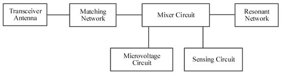
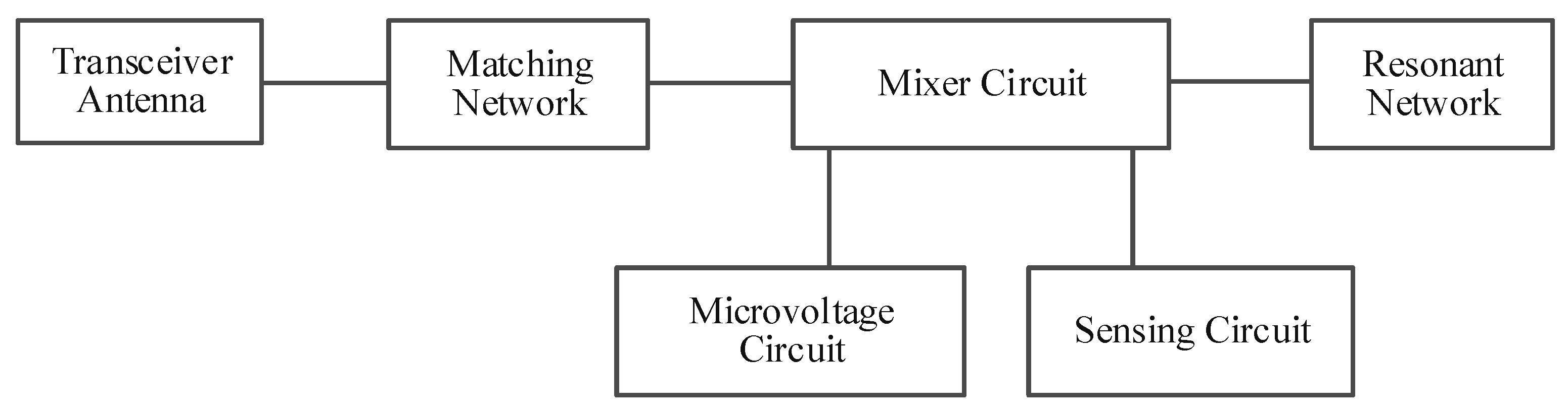
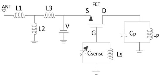
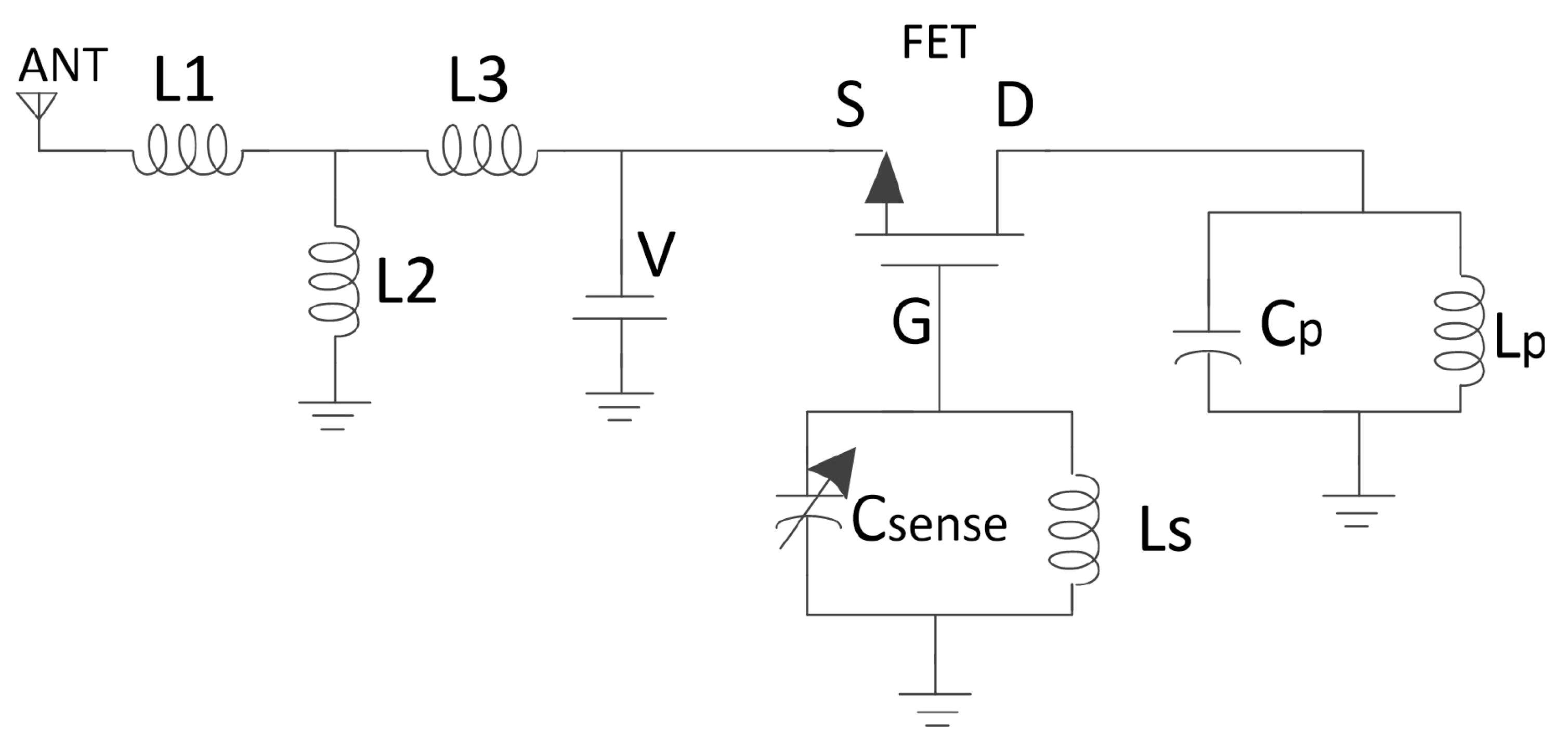
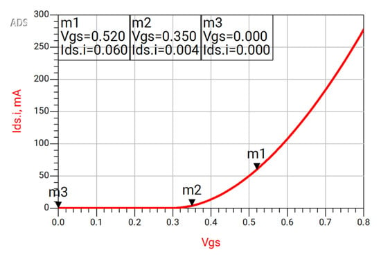
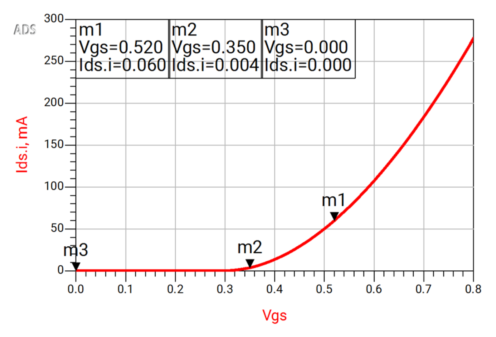
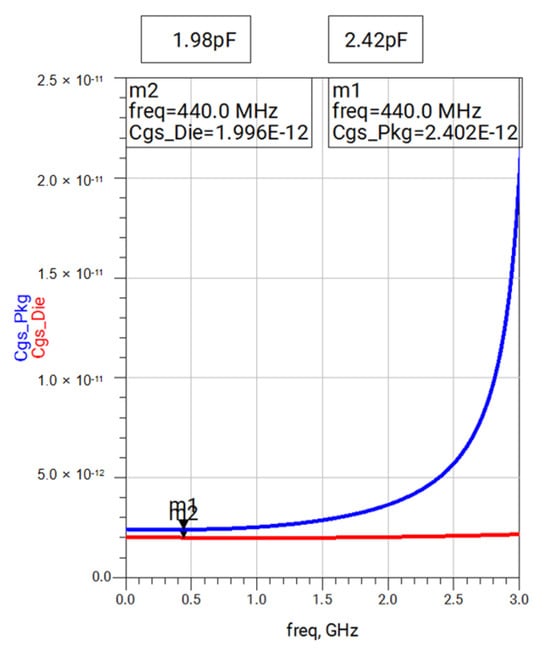
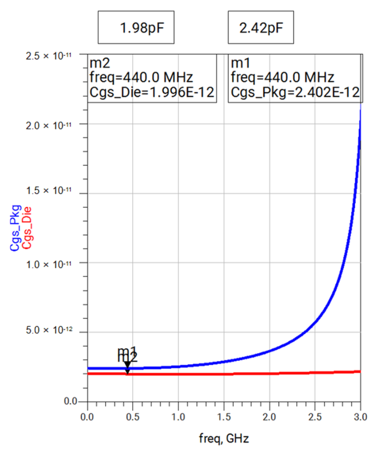
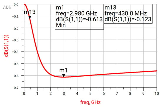
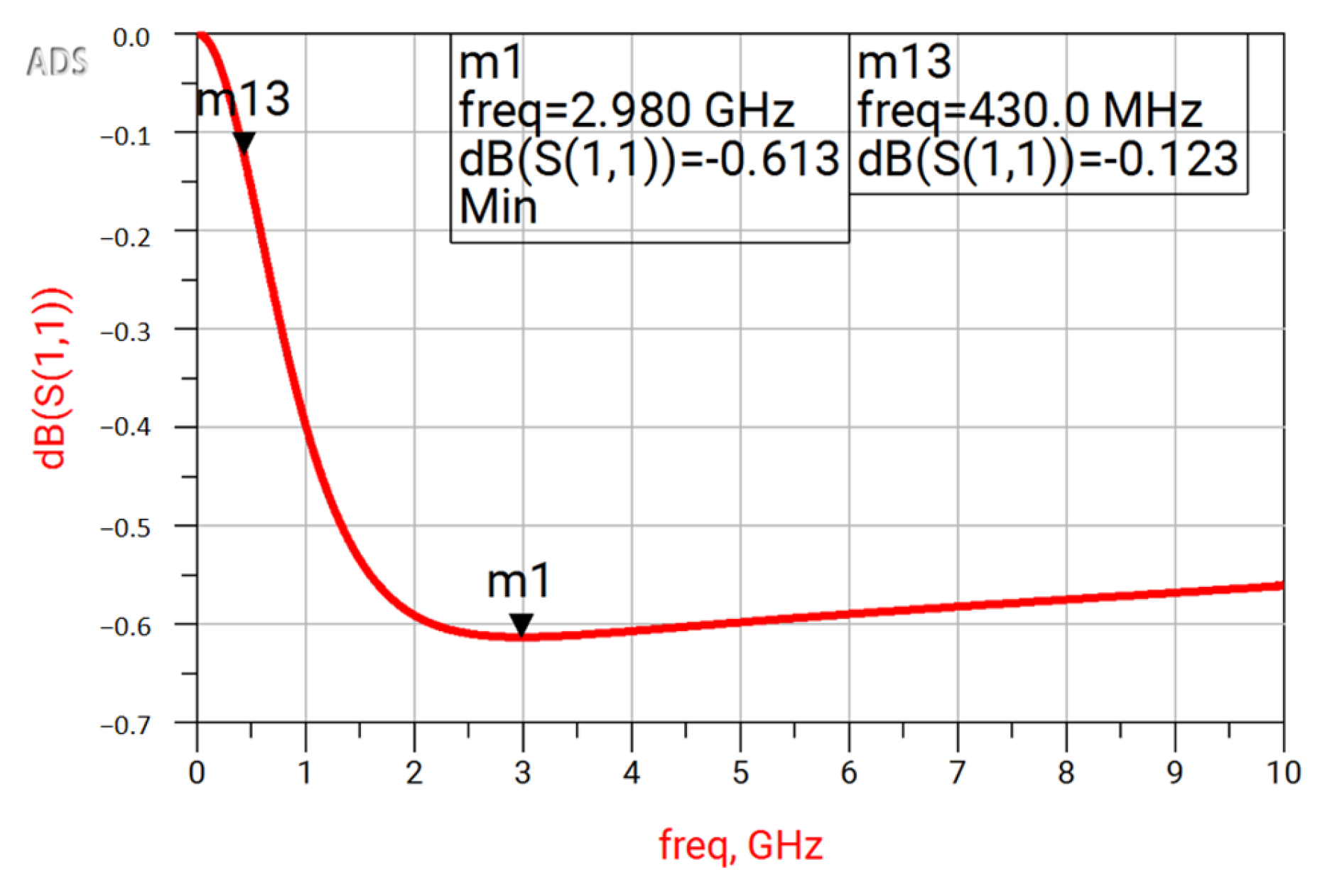
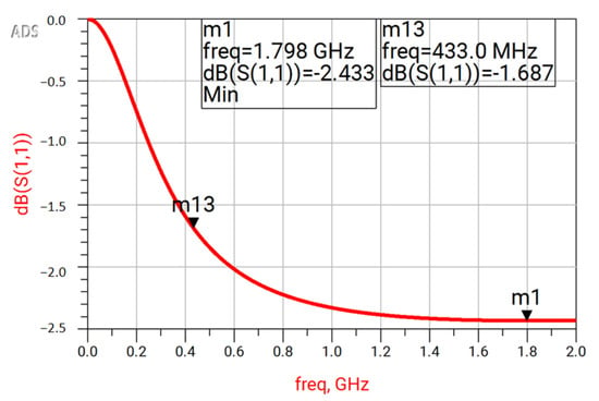
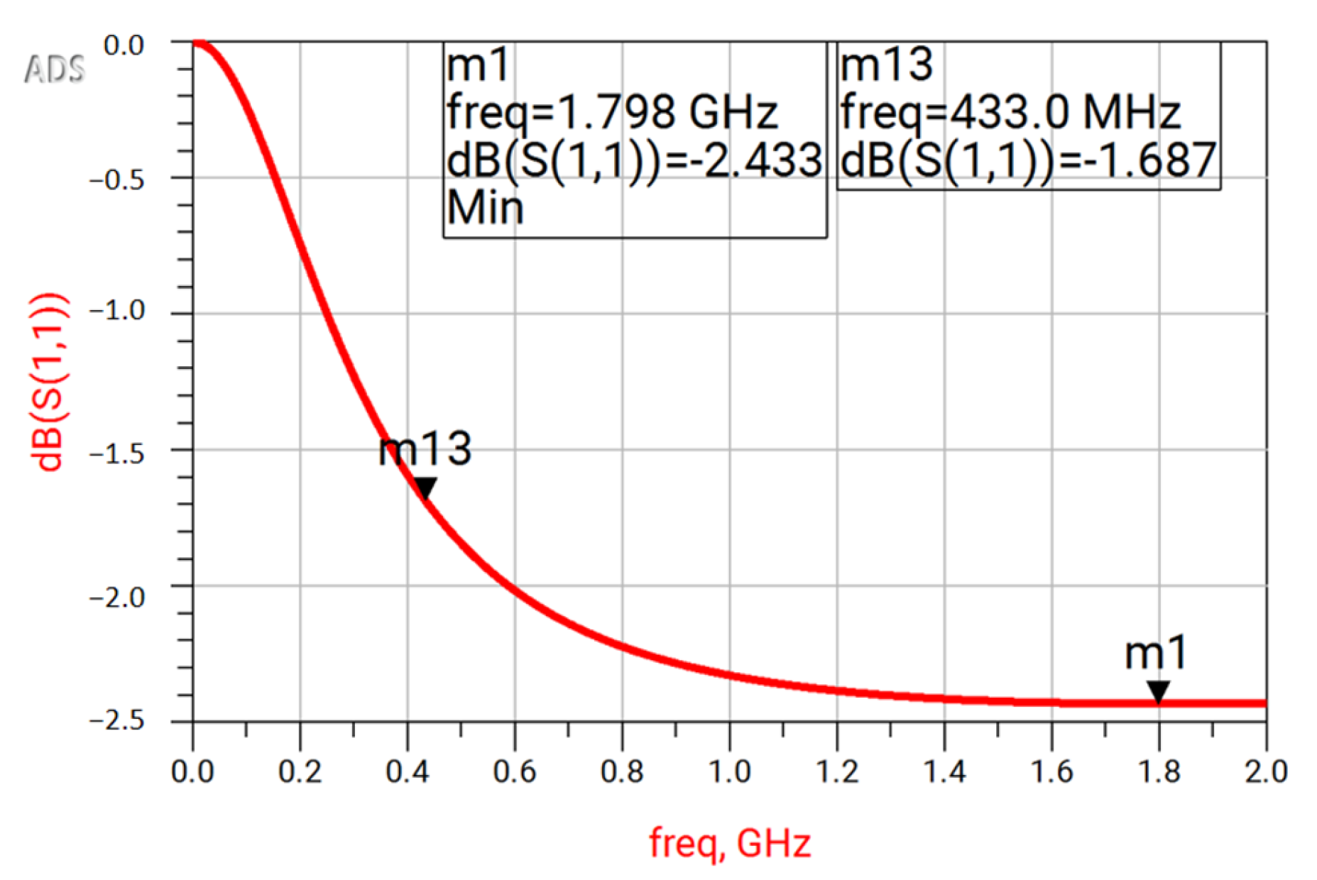
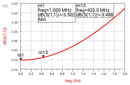
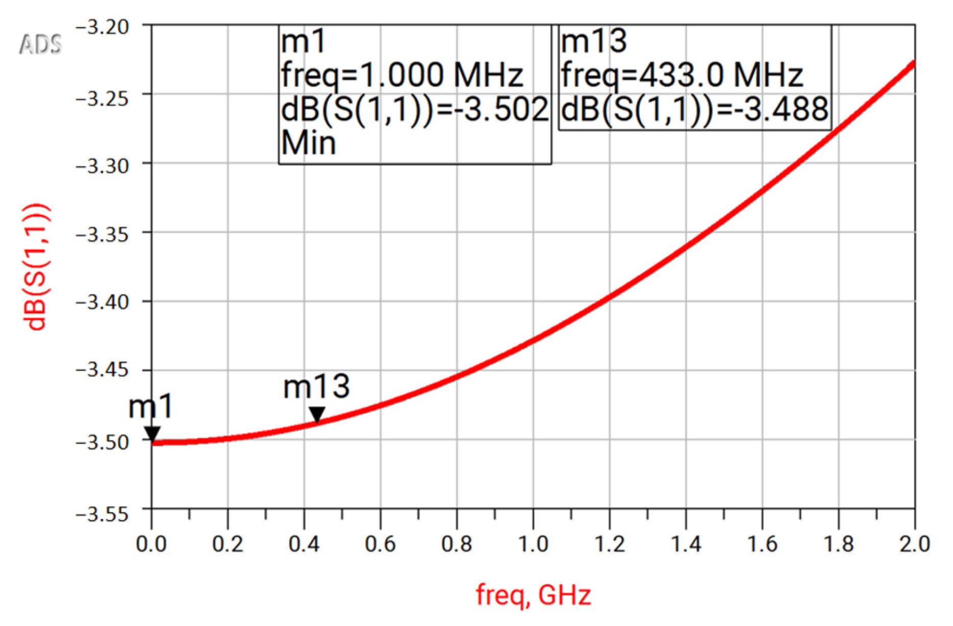
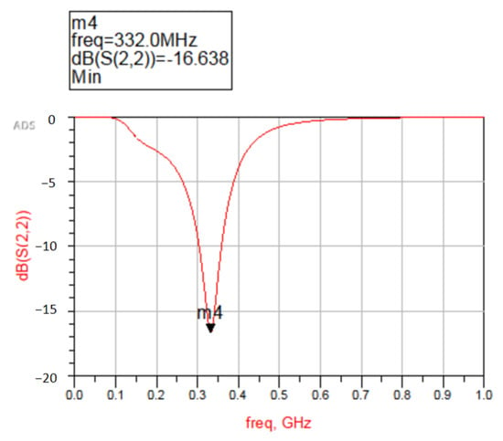
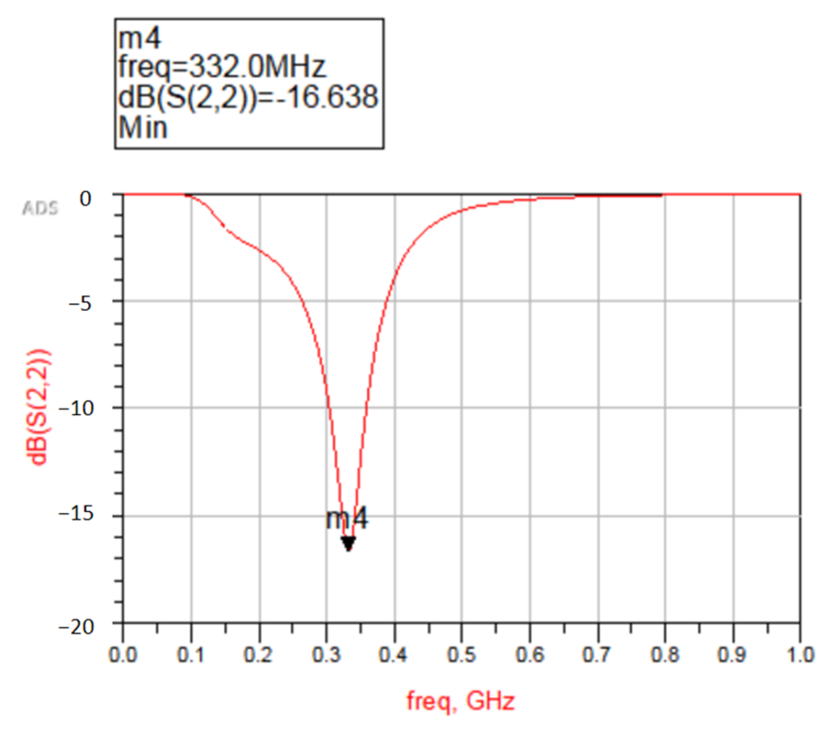
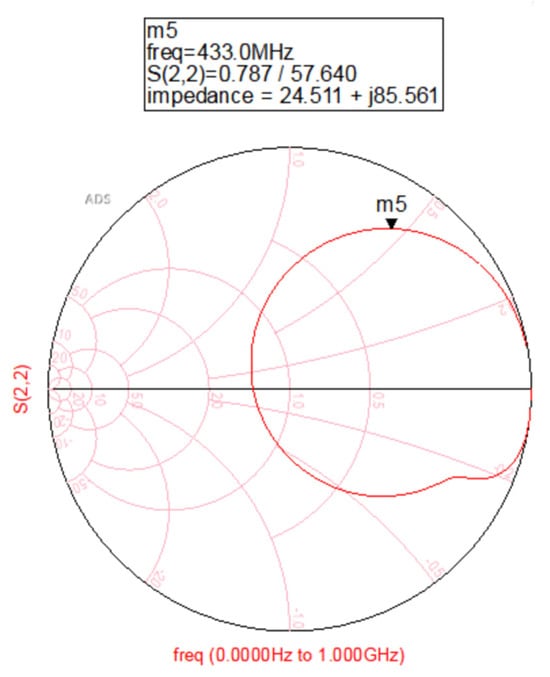
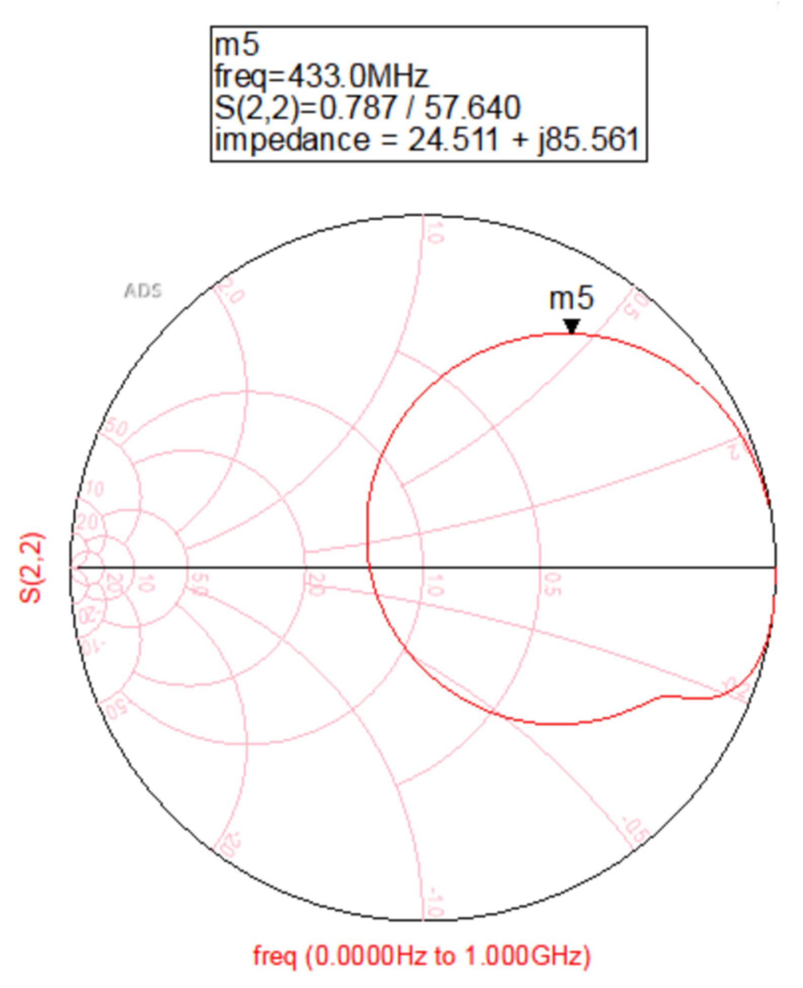
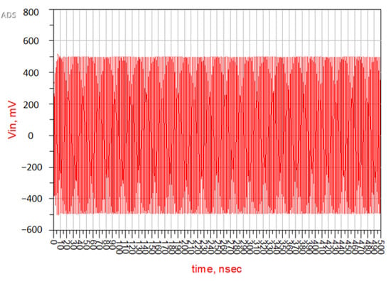
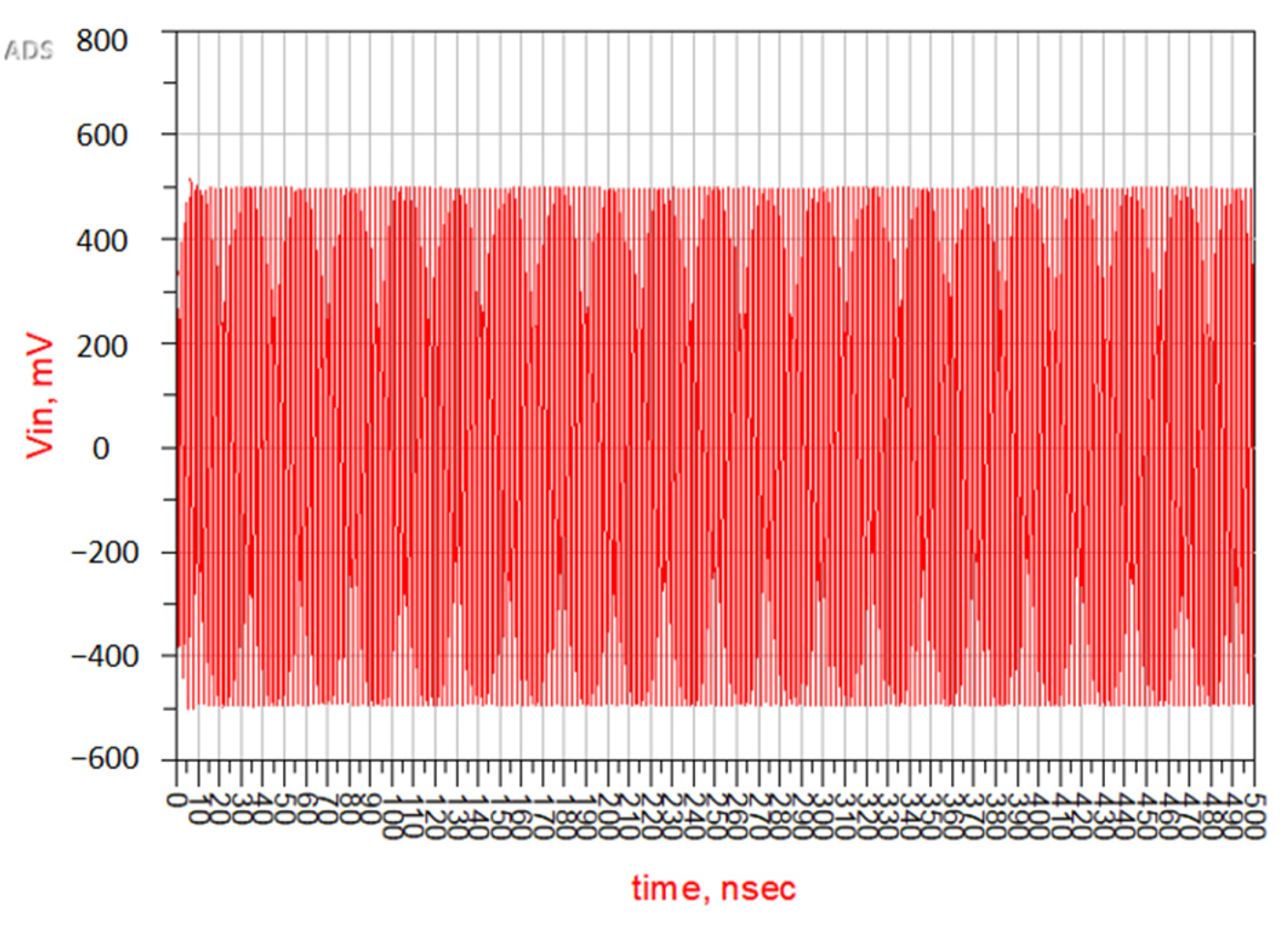
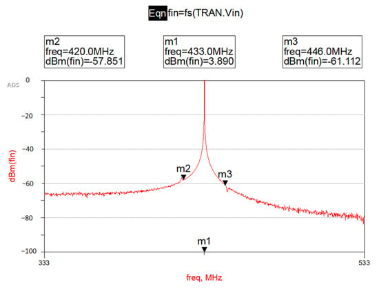
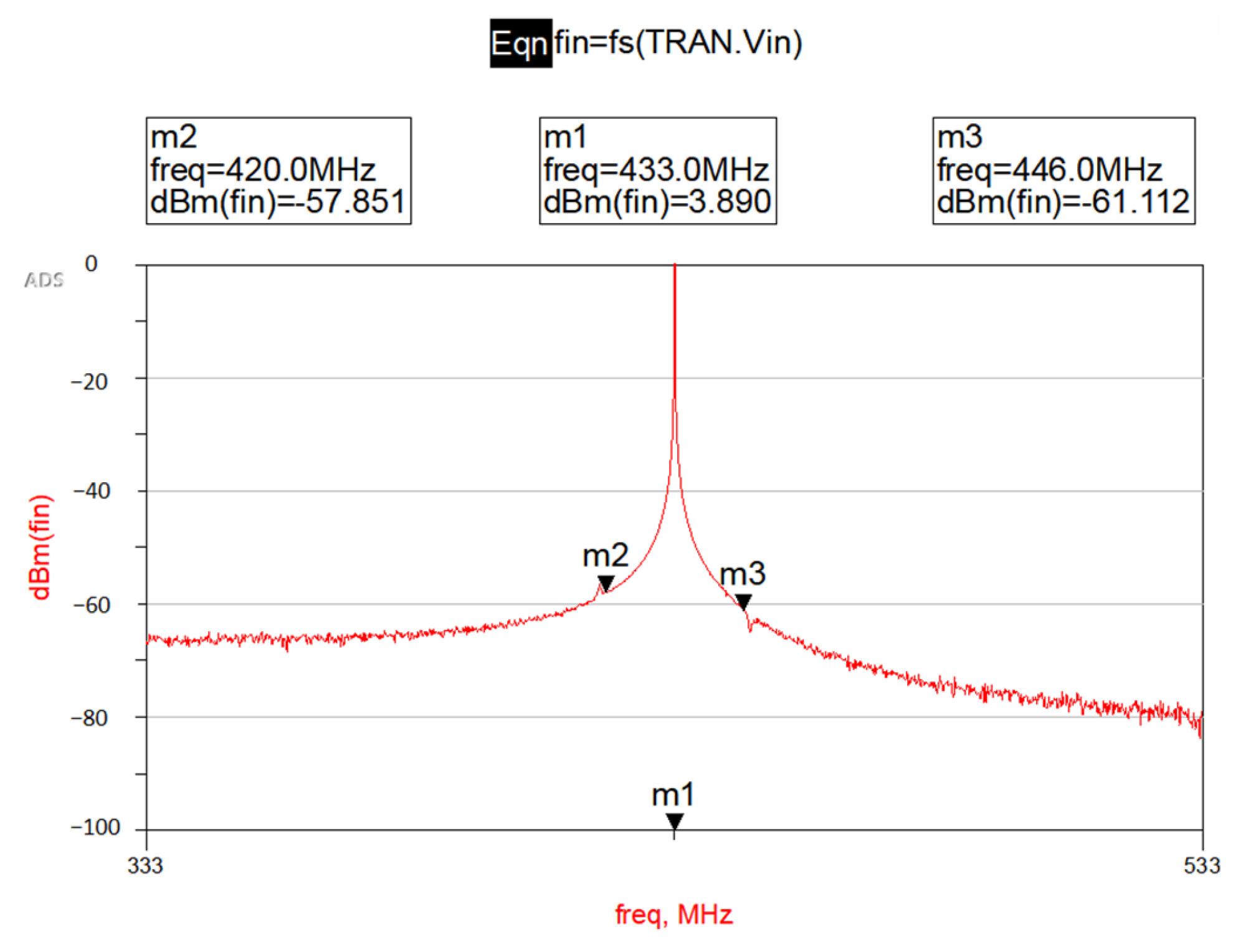
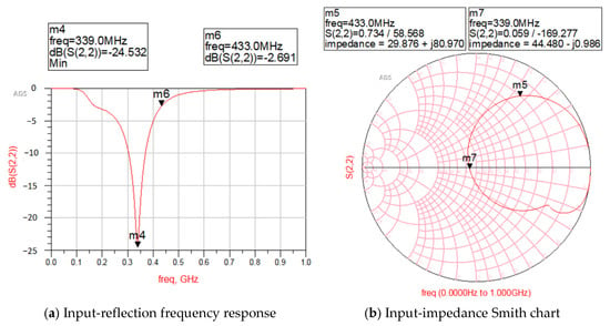
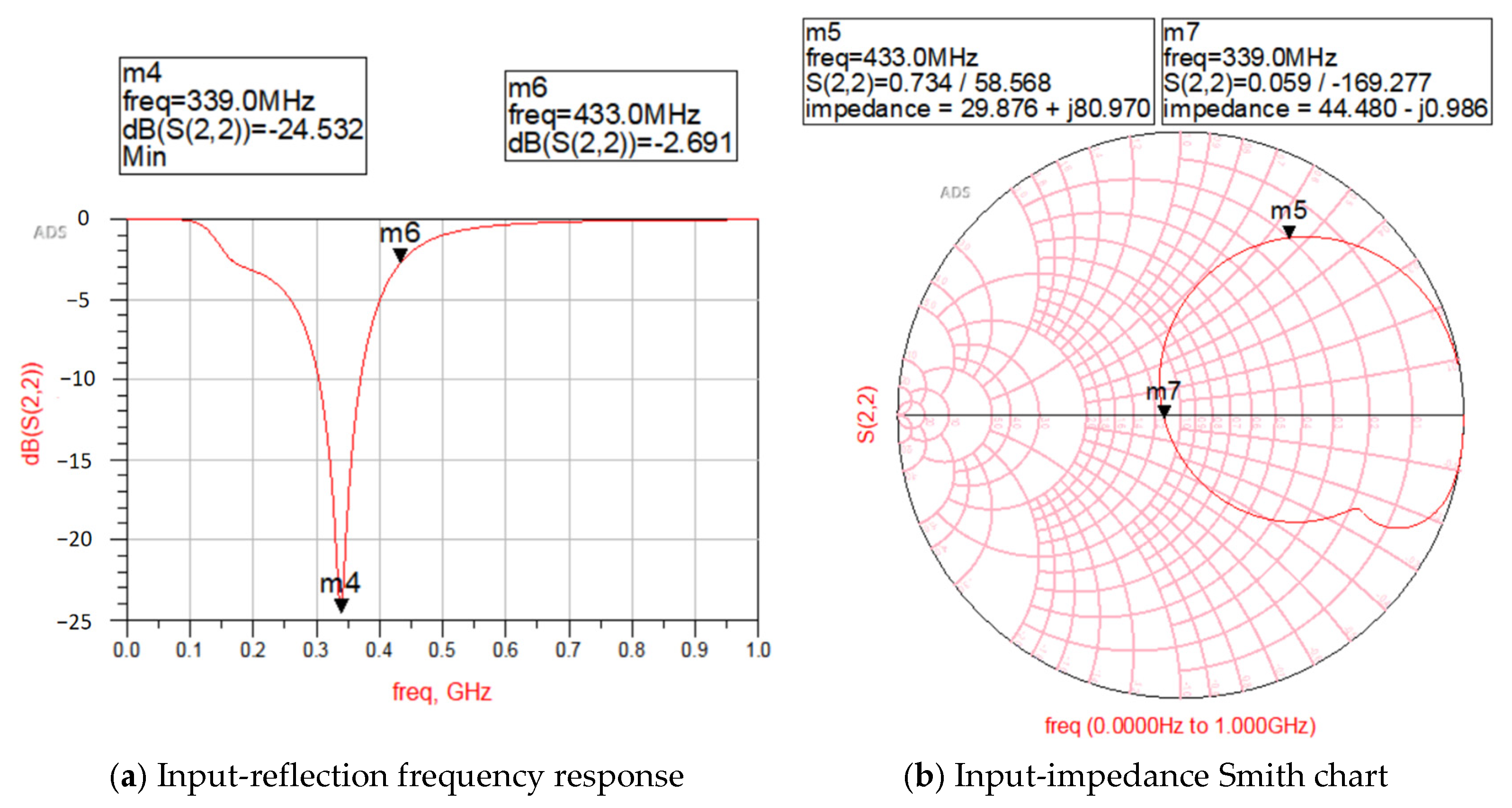
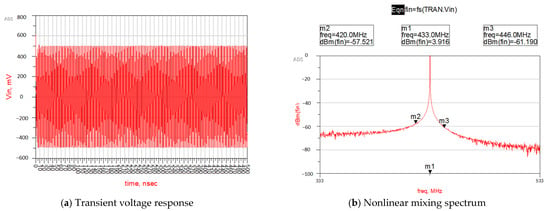
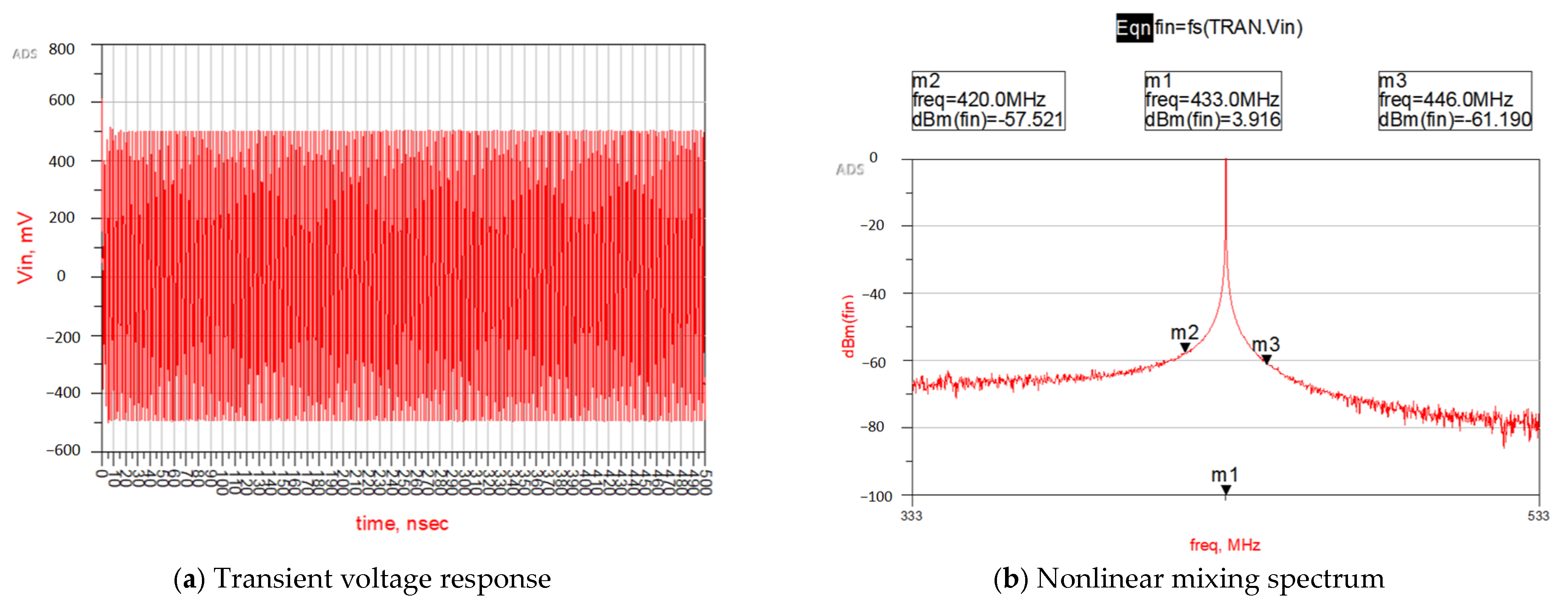
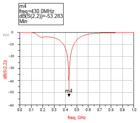
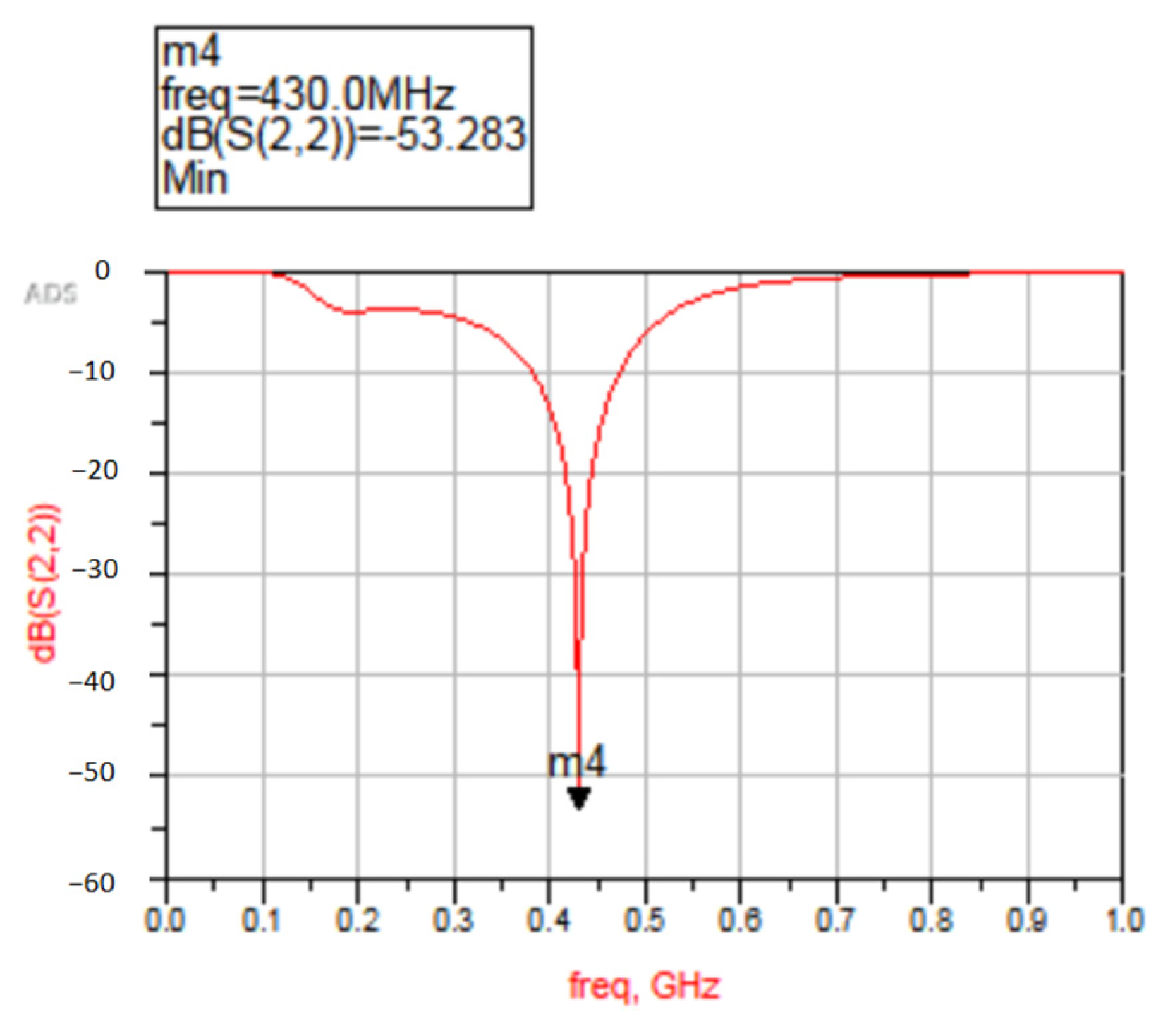
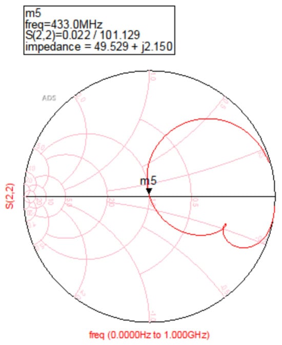
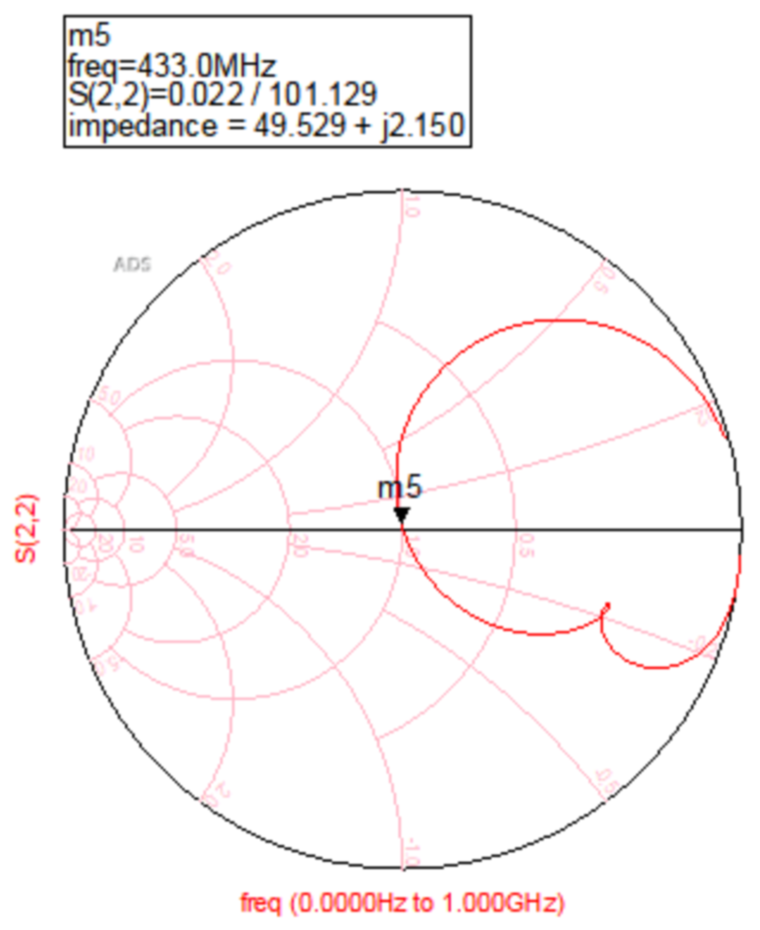
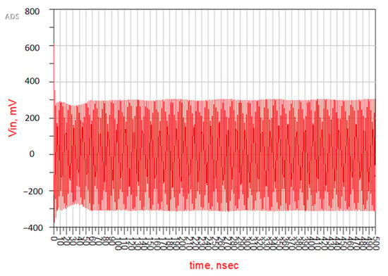
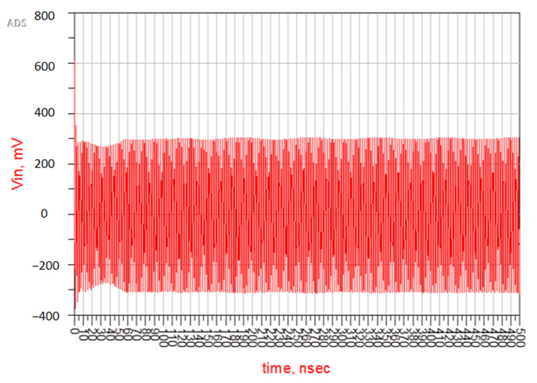
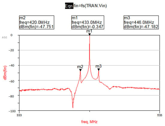
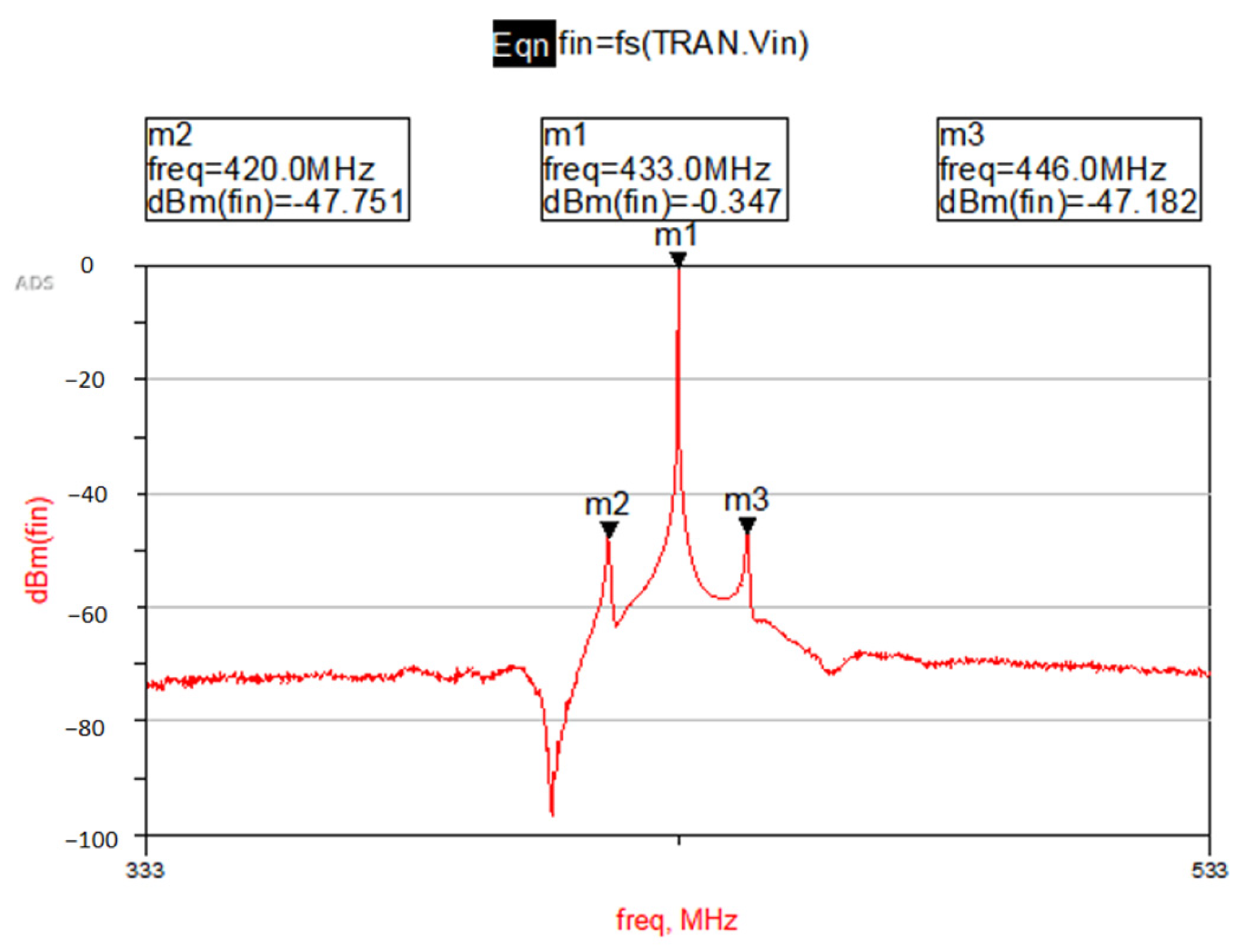
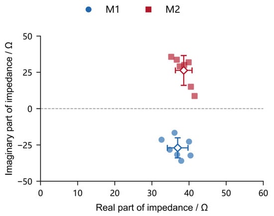
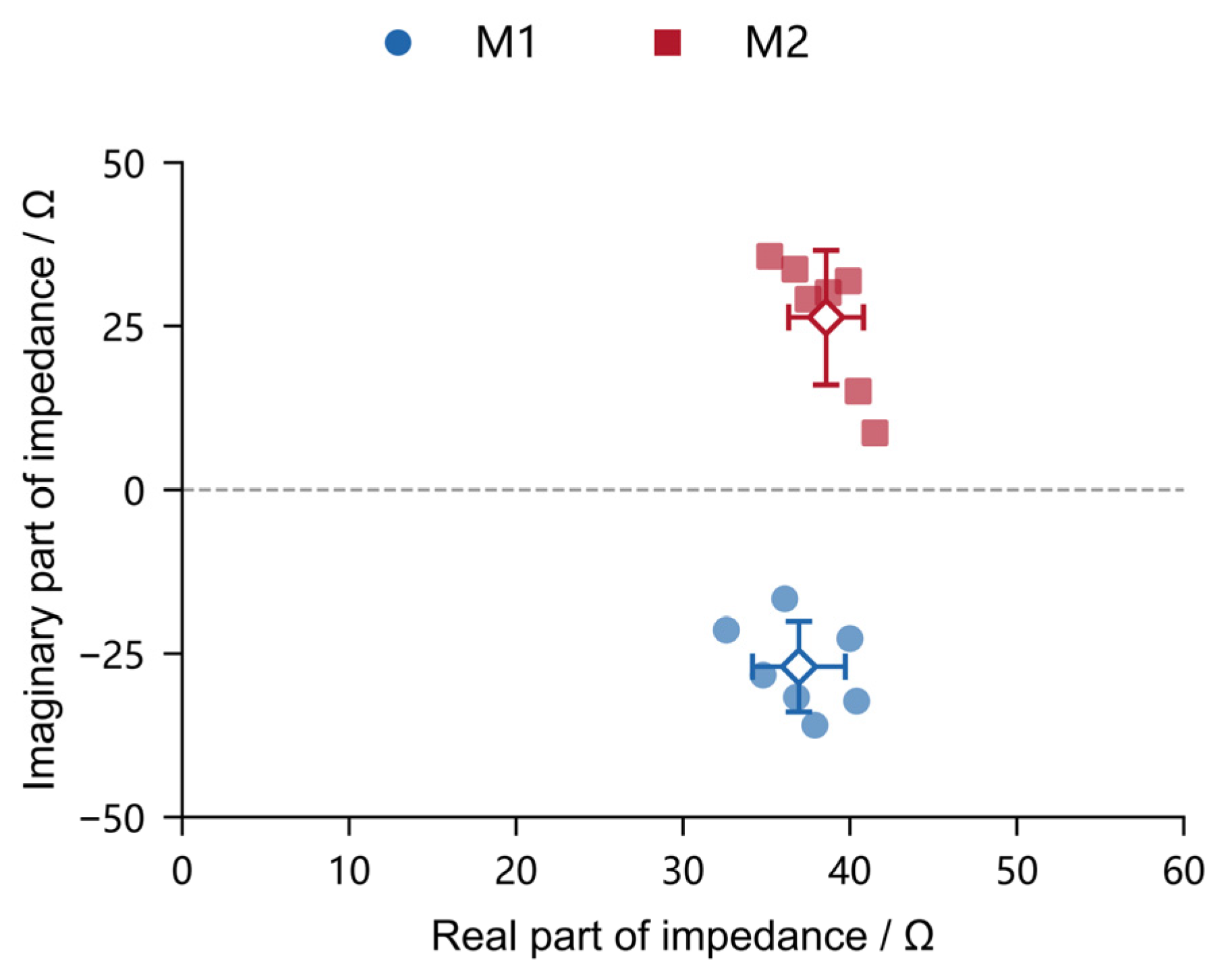
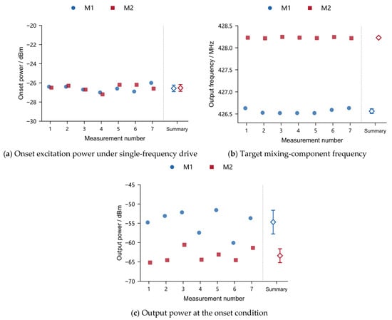
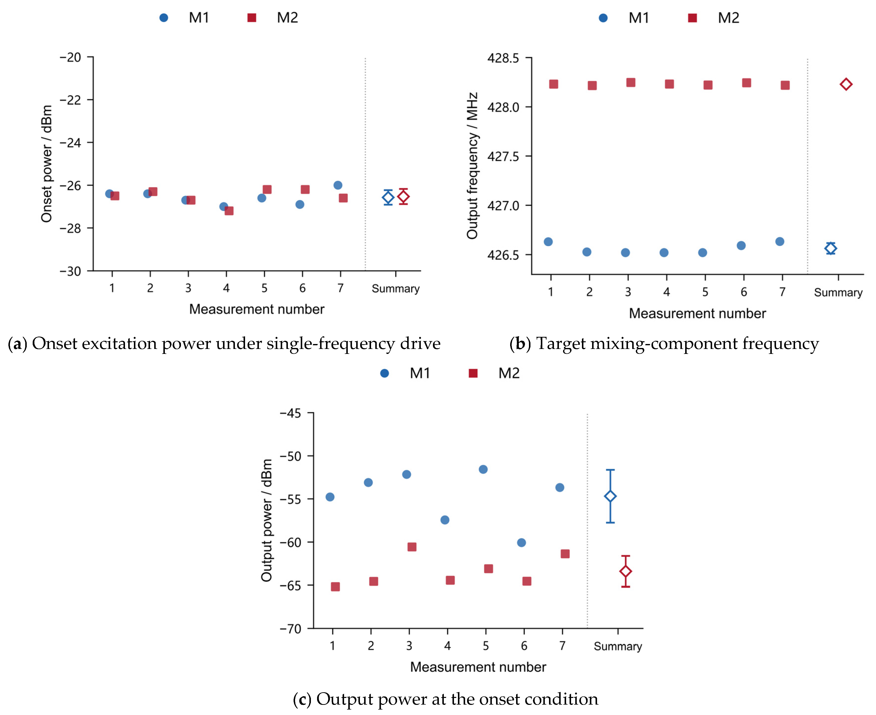
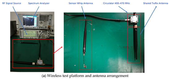
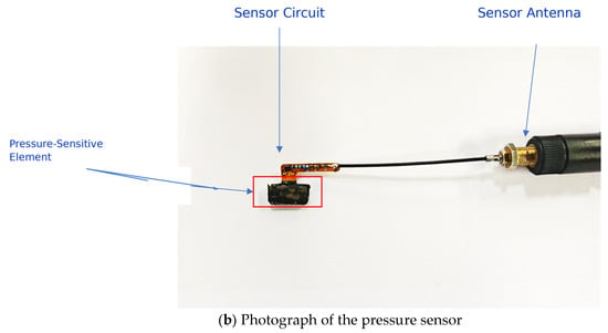
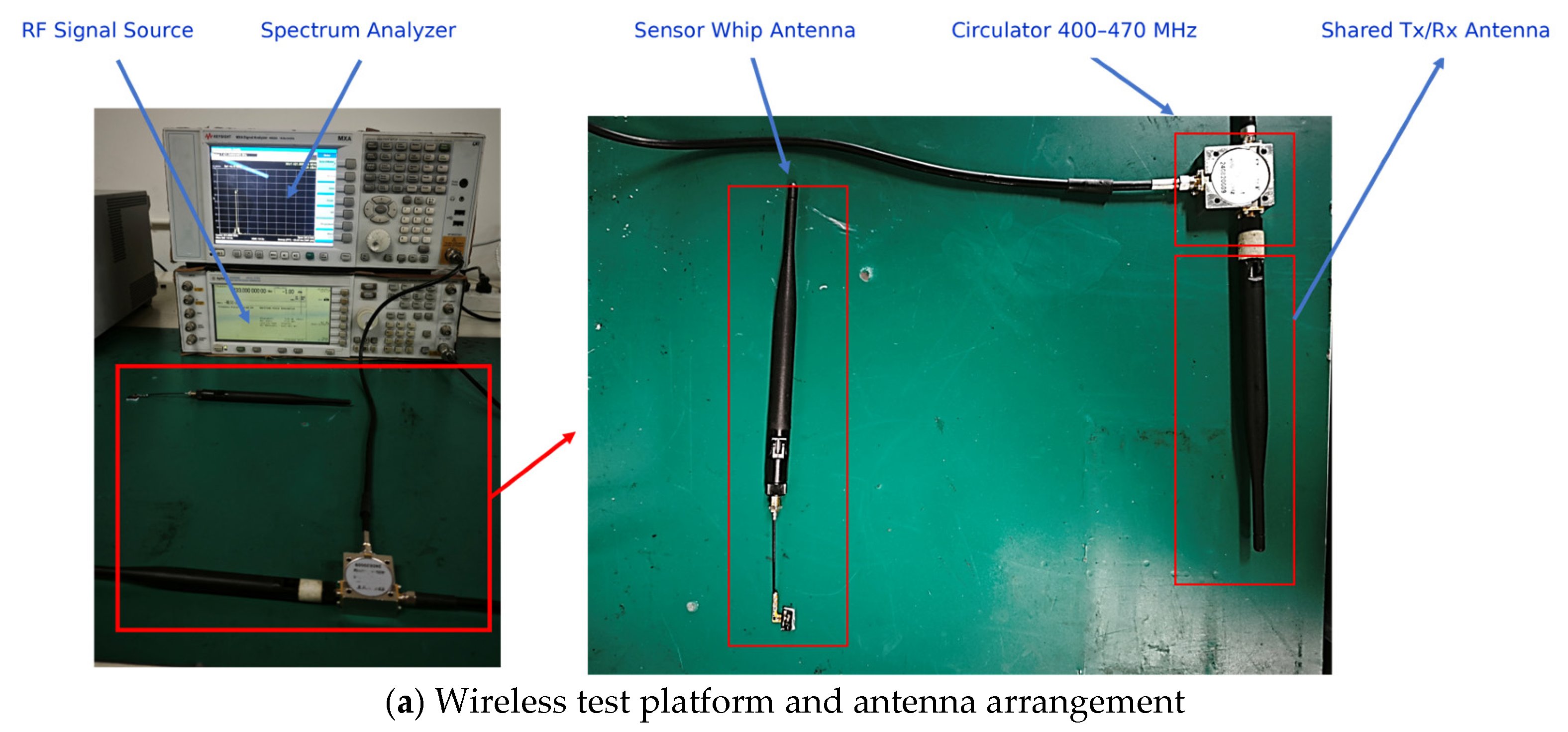
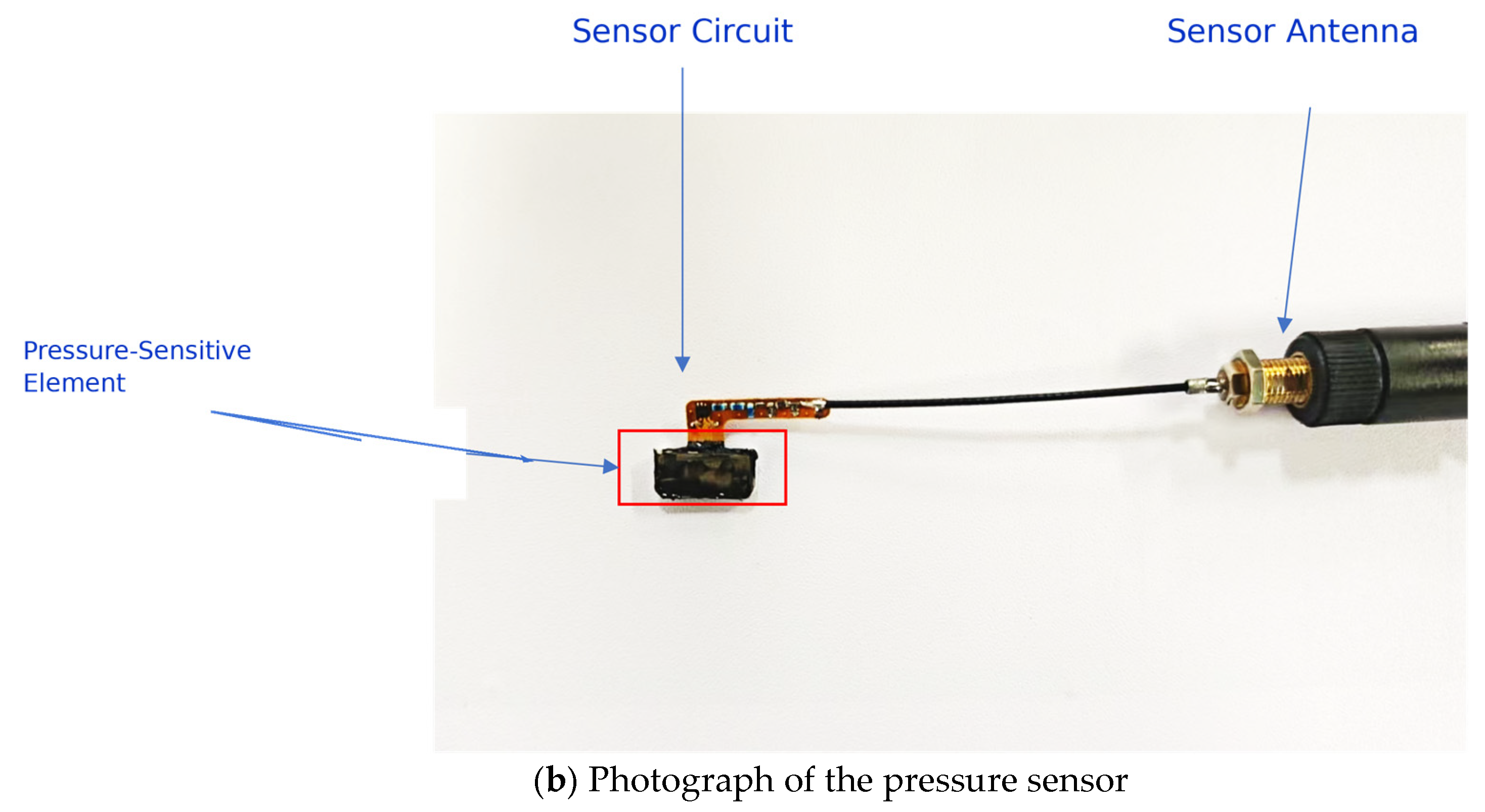
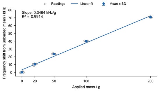
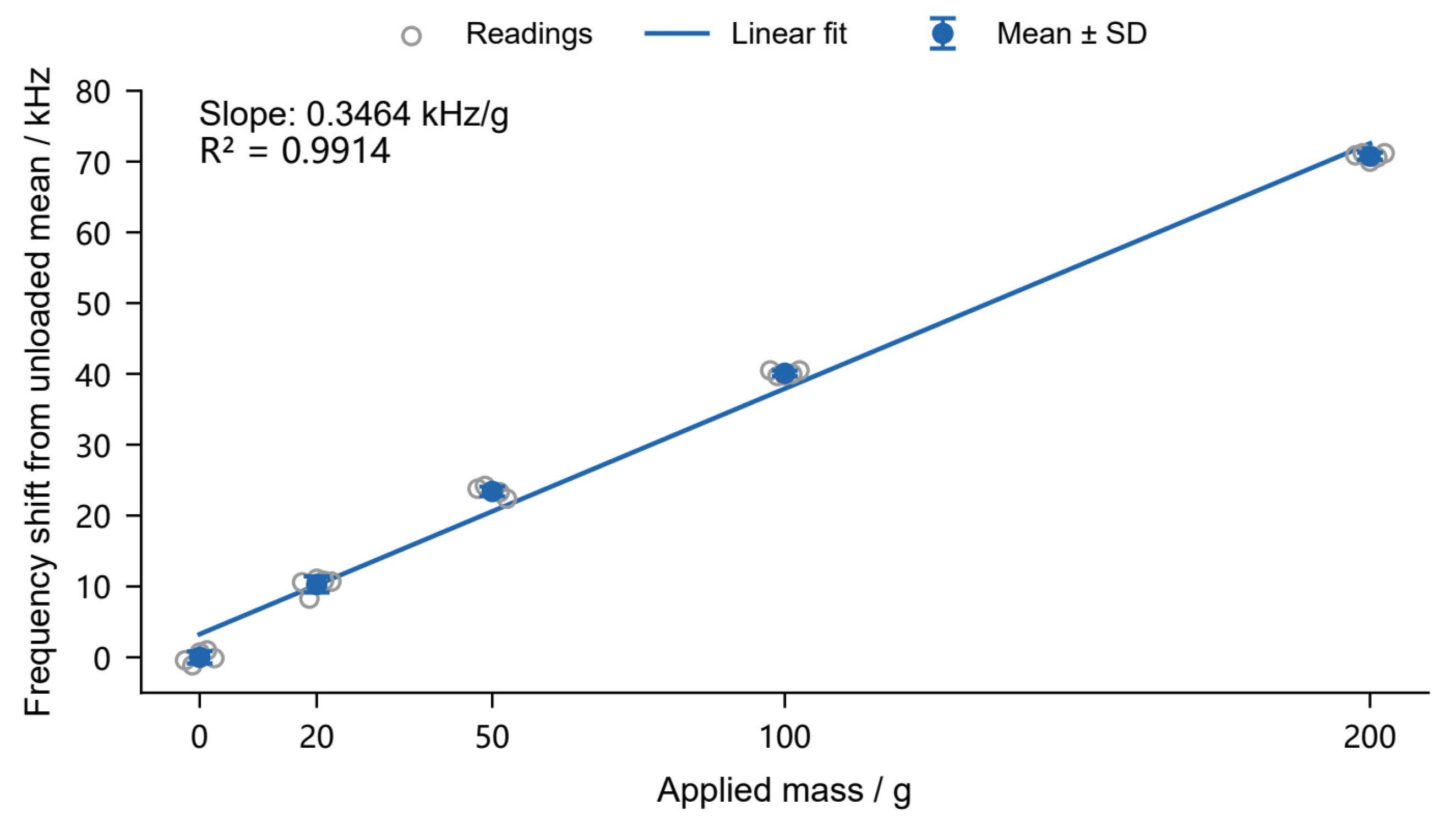

Disclaimer/Publisher’s Note: The statements, opinions and data contained in all publications are solely those of the individual author(s) and contributor(s) and not of MDPI and/or the editor(s). MDPI and/or the editor(s) disclaim responsibility for any injury to people or property resulting from any ideas, methods, instructions or products referred to in the content. |
© 2026 by the authors. Licensee MDPI, Basel, Switzerland. This article is an open access article distributed under the terms and conditions of the Creative Commons Attribution (CC BY) license.