


Abstract
The k-SAT problem is a canonical NP-complete problem for which no efficient algorithm is known. This paper proposes a hybrid quantum–classical search algorithm that employs Grover’s algorithm as the inner local search of a randomized outer loop. Each outer iteration measures a random assignment, prepares a problem-dependent superposition over the Hamming ball of radius r around it, and applies amplitude amplification to locate a satisfying assignment; it returns an assignment rather than a yes/no answer and cannot certify unsatisfiability. Because the ball center is measured, the outer loop remains a classical repetition over independently sampled balls and contributes the inverse success probability rather than its square root; balancing this against the inner quadratic speedup shifts the optimal radius from to and yields the running time , up to polynomial factors— for k = 3, below the best known classical . The contribution is not an asymptotic record—the best known quantum exponents for k-SAT, obtained by amplifying stronger classical solvers as black boxes, remain smaller—but a fully explicit, gate-level construction: the problem-dependent state over the Hamming ball and the k-SAT oracle are decomposed into elementary quantum gates, and the polynomial gate and qubit overheads are accounted for in full.
1. Introduction
The k-SAT problem (k ≥ 3) is a canonical NP-complete problem [1], and no polynomial-time algorithm for it is known. Classical algorithms for k-SAT fall broadly into two categories: deterministic and probabilistic. Deterministic approaches typically rely on divide-and-conquer, exhaustive search, or backtracking, while probabilistic methods often employ local search heuristics. The worst-case time complexity of state-of-the-art algorithms in both categories is generally , where n is the number of Boolean variables, and > 1 is a constant base. Since a smaller implies lower computational complexity, much research [2,3,4] has focused on minimizing this exponential base.
On the probabilistic side, Paturi, Pudlák, and Zane [2] introduced the PPZ algorithm in 1997, achieving a randomized upper bound significantly below . Schöning [3] subsequently proposed a simple local search algorithm with expected running time , yielding , which improved upon the earlier PPZ bound of Ref. [2]. Hofmeister et al. [5] later refined Schöning’s approach, reducing the three-SAT complexity to . Meanwhile, Paturi et al. [6] enhanced the original PPZ framework into the PPSZ algorithm, achieving for unique three-SAT (the variant with exactly one satisfying assignment). Hertli [7] subsequently extended that analysis, proving that the PPSZ bound under the uniqueness assumption applied equally to general three-SAT. More recently, Hansen et al. [8] introduced a biased variant of PPSZ, further improving the unique three-SAT bound to . These algorithms use polynomial working space. Their running time is exponential, and their analyses give the smallest exponential bases known. The analyses do rest on structural assumptions, usually uniqueness of the solution or a bound on the number of satisfying assignments. These assumptions then have to be removed by a separate argument, as in the passage from unique three-SAT to general three-SAT of Ref. [7]. Over two decades of refinements, the base has improved by about two percent over that of far simpler methods: from for the random walk of Ref. [3] to for the biased PPSZ analysis of Ref. [8].
Parallel to these randomized advances, significant effort has been devoted to derandomization and deterministic algorithm design. Dantsin et al. [9] showed how to simulate Schöning’s random walk deterministically, at the price of a mildly larger base: their Hamming-ball local search ran in time , i.e., for k = 3. For three-SAT specifically, they introduced a tailored local search strategy that further reduced the bound to . Moser and Scheder [10] later completed the full derandomization of Schöning’s algorithm using limited independence, and they did so at the price of only an arbitrarily small in the base: their deterministic algorithm ran in time , i.e., for . Brueggemann and Kern [4] refined the local search strategy of Dantsin et al., reducing the three-SAT complexity to . Scheder [11] further improved that bound to . Makino, Tamaki and Yamamoto [12] then derandomized the faster randomized algorithm of Hofmeister, Schöning, Schuler and Watanabe [5] and obtained a deterministic algorithm for three-SAT. The smallest deterministic base for three-SAT is therefore the of Ref. [12]. For general k, it is the of Ref. [10]. Moreover, a deterministic algorithm needs no randomness and no assumption on the instance, and its bounds are reproducible worst-case bounds. What it pays for this is the replacement of the random choices of the probabilistic algorithms by an exhaustive or pseudo-random enumeration. The base is therefore left larger than the randomized one ( against for three-SAT). The deterministic base has come close to the randomized one without going below it, which is why we turn to a different mechanism: a quadratic speedup inside the ball, which changes the base rather than refining the classical search.
Quantum algorithms have demonstrated advantages over classical counterparts in several computational tasks, including integer factorization, unstructured search, and search on graphs [13,14,15], and they are studied as a tool for application areas ranging from machine learning to combinatorial optimization [16,17,18].
Hybrid quantum–classical schemes have become the standard way of exploiting quantum resources while devices remain small. In such a scheme, a classical outer loop calls a quantum subroutine. The optimization landscape of this family is reviewed in Ref. [19]. Such algorithms can be implemented on near-term hardware with few qubits and shallow circuits and are assessed by the quality of the solution that the classical optimizer reaches. In addition, a related line of work embeds quantum or quantum-inspired search into a classical metaheuristic. Nardin and D’Andreagiovanni [20], for instance, combine a quantum-inspired ant colony optimization with exact local searches that guarantee convergence to an optimum within a suitable solution neighborhood. The method works on structured combinatorial problems and is validated empirically. Grover-type search has also been adapted to combinatorial problems through dedicated state preparations and oracles. Examples are a simplified quantum counter for the exact cover problem [21] and Dicke-state search for vertex cover [22]. Hybrid schemes have further been proposed for continuous optimization [23], text search [24] and reconfigurable quantum–classical computing frameworks [25]. These works address other aspects of hybrid schemes (implementability on near-term devices, empirical performance on structured problems, dedicated state preparations and oracles) rather than the quantity analyzed in this paper, namely, the exponent of the total cost of the hybrid with the classical repetitions included; each is cited as an example of one line of work in the family to which the present scheme belongs, and that is the use made of them here. These works show how a quantum subroutine can be inserted into a classical search while keeping the quantum resource small. Ref. [26] optimizes such a hybrid method as a whole, and it is the one taken up next.
Among the hybrid schemes for combinatorial optimization, the one closest in approach to the present work is Ref. [26], which also solves three-SAT with a hybrid quantum–classical algorithm. It asks whether a quantum computer of Q qubits can speed up a computation on variables, a question motivated by the size of near-term devices, and shows that it can, by exhibiting a hybrid algorithm faster than its fully classical counterpart. Four points separate the two contributions. (i) Model of the device, and the question asked. Ref. [26] imposes a size restriction (the device is much smaller than the instance) and asks whether a speedup exists under it. Here, no size restriction is imposed (the device must hold the n assignment qubits together with polynomially many ancillas), and the question is quantitative: What exponent does an explicit construction achieve for every (Ref. [26] treats three-SAT), and how must the classical outer loop and the quantum inner loop be balanced to obtain it? (ii) What is designed. Both works search a Hamming ball of radius around a center, and both balance the number of balls, , against the cost of the search inside one ball. Ref. [26] writes out that balance as well and optimizes it for a classical ball search, obtaining for the radius of Ref. [9] and of Ref. [3]. There, however, the radius that the quantum routine can handle is capped by the device ( for qubits), so the optimum of the balance with a quantum inner search is not attainable in that model. Here, no such cap is imposed: because the center of each ball is measured, the outer loop stays classical and contributes the inverse success probability rather than its square root, and re-balancing that factor against the cost of the inner amplitude amplification moves the radius to its own optimum, , which fixes the exponent (Section 3.7). The radius is thus fixed by the optimization, not by the size of the device. (iii) Where the quantum search is placed. In Ref. [26] the quantum routine is inserted at the bottom of a classical recursion: the ball search recurses with a decreasing radius, and the device is called once the radius is small enough to fit into Q qubits, hence the effort that reference spends on compressing the branch register into qubits. Here, the whole ball of radius is searched coherently within one run. The tree is in both cases the clause-driven one, selected at each round by the first unsatisfied clause. What the present work adds is the bound on the marked amplitude: a leaf of depth d carries amplitude , so the state of Equation (6) has amplitude at least on the satisfying assignments, and reflecting about that state rather than about the uniform superposition is what fixes the polynomial overhead (Section 3.5 and Section 3.7). (iv) What is established. Ref. [26] establishes that a polynomial speedup over Schöning’s algorithm survives for a device of any constant fraction of the instance size; the radius is in that case fixed by the device, and the exponent is expressed relative to Schöning’s, as . By contrast, the present paper removes the size restriction and evaluates the same balance at its own optimum, which yields the exponent in closed form for every k≥ 3: it gives a gate-level decomposition of the state preparation and of the k-SAT oracle (Section 3.3 and Section 3.4), counts the polynomial overhead in full (Section 3.7) and checks numerically the two bounds on which the exponent rests (Section 4). Stated positively, the two works share the idea of placing amplitude amplification inside a Hamming-ball search; what the present work adds is the three points (ii) to (iv), namely, the radius fixed by the optimization rather than by the size of the device, together with the closed-form exponent obtained at that radius for every and the explicit construction with the two bounds verified numerically. The two works are complementary rather than competing: Ref. [26] asks what a device of a given size can still achieve, the present paper what the construction achieves once the size restriction is removed.
Motivated by these developments, we investigate the application of quantum computation to the k-SAT problem. Prior quantum approaches to k-SAT largely accelerate an existing classical solver while keeping its structure inside a black-box oracle. Grover’s algorithm alone yields [14]. Combining Grover search with the then best classical three-SAT algorithm ( [5]) lowers the exponent to [27], and applying amplitude amplification [28] to the PPSZ algorithm [6,7,8] gives for three-SAT. These are, to our knowledge, the strongest known exponents for worst-case three-SAT in the gate model. Inspired by the classical algorithm in [3], we propose a hybrid quantum–classical algorithm that employs Grover’s algorithm as a local search subroutine for solving k-SAT. The proposed algorithm is a hybrid quantum–classical procedure: its outer loop classically samples local search spaces, while its inner loop performs quantum search. It proceeds in t outer iterations. In each iteration, a problem-dependent superposition state is constructed over a local search space—specifically, a Hamming ball of radius r centered at a randomly generated assignment—by exploiting the problem structure. Grover’s algorithm is then applied to that state in its amplitude-amplification form—the number of solutions inside a ball is not known in advance, so the exponential-search variant is used—to search for a satisfying assignment. Because the outer loop is a classical repetition over independently sampled balls, the number of outer iterations is governed by the classical success probability, and the resulting running time is (with the optimal radius ), which improves upon the classical local-search bounds for k-SAT [3,9] and, at k = 3, upon the best known classical algorithm [8] ( versus ; see Section 3.9 for the general-k comparison). These gains are over classical solvers: black-box amplification of a stronger classical solver yields smaller quantum exponents [6,8,27,28].
The contributions of this work can be summarized as follows.
- An explicit, gate-level construction. Both the problem-dependent superposition over the Hamming ball and the k-SAT oracle are decomposed into elementary gates, so that no black-box oracle is left in the complexity and the polynomial overhead is fixed at gates.
- A hybrid framework with a re-optimized ball radius. Because the center of each ball is measured, the outer loop is a classical repetition over independently sampled balls and contributes the inverse success probability rather than its square root; balancing this factor against the quadratic speedup of the inner search shifts the optimal radius from the classical to , so that the classical repetition does not simply reproduce the classical Hamming-ball exponent.
- A complete accounting and a numerical verification. The qubit and gate costs of the whole construction are counted, and the two bounds on which the exponent rests—the success probability of a ball and the marked amplitude of the constructed state—are checked numerically for on small instances (Section 4).
- A precise statement of what the algorithm computes, and of how robust it is. The procedure is a search algorithm: it returns a classically verifiable satisfying assignment and never certifies unsatisfiability (Section 3.6). The effect of state-preparation and gate errors on the success probability is quantified, and the assumptions needed for a reliable implementation are listed. The quantum and classical resources are counted explicitly (Section 3.8). Finally, the numerical verification is extended to instance classes with few satisfying assignments, where the worst-case amplitude bound is nearly tight (Section 4).
The remainder of this paper is organized as follows. Section 2 introduces the k-SAT problem, defines quantum analogs of the three fundamental classical logic gates involved, and reviews Grover’s algorithm. Section 3 presents the proposed algorithm, beginning with an overview of the framework, followed by the construction of the problem-dependent state and the decomposition of the Grover oracle for k-SAT into elementary quantum gates. The section concludes with an analysis of the algorithm’s feasibility and time complexity and with a comparison against prior quantum algorithms and additionally provides the pseudocode of the complete procedure (Section 3.2), a precise statement of the problem the algorithm solves (Section 3.6) and an analysis of its robustness to state-preparation and gate errors together with the full resource accounting (Section 3.8). Section 4 reports the numerical verification of the two bounds entering the exponent, on planted instances as well as on instance classes with few satisfying assignments; Section 5 offers concluding remarks, including the limitations of the study and directions for future work, and the Appendix A details the gate-level implementation of the conditional neighborhood expansion.
2. Preliminaries
2.1. Definition of the k-SAT Problem
The k-SAT problem in conjunctive normal form (CNF) is defined as follows. Let be a finite set of n Boolean variables, and let be a set of m clauses. Each clause is given by , where each is called a literal; for simplicity, the k literals of a clause are assumed to involve k distinct variables, so that no clause contains both and . This is the case considered throughout, and it is what makes the k branches generated by [Equation (5)] distinct. The k-SAT problem asks whether there exists an assignment, such that the formula is satisfied. If is satisfied by a, then a is called a satisfying assignment of .
Note that for fixed n and m, each distinct set of clauses defines a unique instance of the k-SAT problem. Throughout, m is taken to be polynomially bounded in n, so that the clause count contributes only a polynomial factor to all running times reported below. In classical computation, a Boolean variable takes a binary value of either zero (false) or one (true), and logical operations act on one or more such variables. By analogy, a quantum truth value can be defined as a superposition of the basis states and . A quantum logical variable assumes such a quantum truth value and is naturally represented by a qubit, whose state encodes that value. Consequently, a quantum logical operation is defined as a quantum gate acting on one or more qubits, transforming their joint quantum state.
The k-SAT problem involves n Boolean variables, each taking a value in . Consequently, there are possible assignments, which constitute the search space . Each assignment can be encoded as a computational basis state , where . In the remainder of this paper, we identify each classical assignment with its corresponding computational basis state.
2.2. Quantum Realizations of Logic Gates: NOT, AND, and OR
As shown above, the k-SAT problem is built upon three basic logical operations: (∧), (∨), and (¬). Their quantum analogs, denoted as , , and , are defined as follows.
The classical operation maps and . Its quantum analog, , is defined by its action on the computational basis:
This operator is equivalent to the single-qubit Pauli-X gate, which flips .
The classical gate () embeds into a reversible three-qubit operator :
This is precisely the Toffoli gate, which applies a bit-flip to the third qubit if and only if the first two qubits are both .
The classical operation acts on two Boolean variables, yielding zero if and only if both inputs are zero. Its reversible quantum analog, , is defined on three qubits as:
where ⊕ denotes addition modulo two. This operation flips the target qubit conditioned on at least one of the control qubits or being one. The gate can be implemented via and . Specifically, one applies to each of the first two qubits, then to all three qubits, and finally to each of the three qubits.
2.3. Grover’s Algorithm
In Grover’s algorithm, the Grover iteration is applied times to the system state, where is the search space size (n being the number of qubits) and M is the number of solutions. The qubits are then measured in the computational basis, which returns a solution with probability ; repeating the whole procedure times raises the success probability to at least .
The Grover iteration consists of the following four steps:
- Apply the oracle O: , where if x is a solution and otherwise. This marks the solution states by flipping their phases.
- Apply the Hadamard transform .
- Apply the diffusion operator , which reflects the state about (equivalently, flips the phase of all non-zero computational basis states).
- Apply the Hadamard transform .
Using the identity , where is the equal superposition state, the Grover iteration simplifies to
where O is the oracle defined in Step 1.
If an oracle is available that marks the solution states of a given problem, Grover’s algorithm can solve it without exploiting additional problem-specific structure beyond the oracle itself. In particular, for the k-SAT problem, assuming such an oracle exists and the instance has a unique solution (), Grover’s algorithm achieves a time complexity of . This provides a quadratic speedup over exhaustive classical search; it does not, however, beat the classical bounds of Section 1: for , its base lies above the deterministic of Ref. [12] and above the randomized of Ref. [8], as Table 1 also records. Nevertheless, incorporating problem structure into the quantum algorithm can further reduce the complexity, as demonstrated in the subsequent analysis.
Table 1.
Exponential base in the gate-model running time for worst-case 3-SAT. The first two rows are classical reference points included for comparison; the remaining rows are quantum gate-model algorithms.
3. The Proposed Algorithm
3.1. Algorithm Framework
The proposed algorithm is a hybrid quantum–classical procedure whose outer loop performs t classically repeated iterations, each consisting of the following three steps:
- Random assignment generation. Prepare the uniform superposition state by applying to n qubits initialized in , then measure all qubits in the computational basis to obtain a random assignment .
- Subspace state preparation. Construct a problem-dependent quantum state starting from the randomly generated assignment .
- Grover search within subspace. Apply Grover’s algorithm to to search for a solution to the k-SAT instance. The number of solutions inside a ball is not known in advance, so the exponential-search variant of amplitude amplification is used, as in Step 3 of Algorithm 1 (Section 3.2).
| Algorithm 1 Hybrid quantum–classical k-SAT search. |
| Input: a k-CNF formula with n variables and m clauses; radius ; , the number of trials that brings the success probability to ; failure tolerance ; total number of trials , where the constant absorbs the (rather than unit) success probability of the amplification of Step 3. Output: a satisfying assignment of , or fail. Repeat Steps 1–4 for ; the T trials are independent classical repetitions of the same procedure.
|
3.2. Pseudocode of the Complete Procedure
Algorithm 1 collects the three steps of Section 3.1 into a single procedure and marks which operations are quantum, which are classical, and where the two meet. Step 1 is a measurement: the center a is a classical bit string. The T repetitions of the loop are therefore independent classical trials, and the loop contributes the inverse success probability rather than its square root. This is what fixes the optimal radius at in Section 3.7. Steps 2 and 3 are performed coherently: the r rounds of state preparation, the J amplitude-amplification iterations and the oracle calls of one round are executed without intermediate measurement, the only measurements being the intermediate checks of the exponential-search schedule of Step 3 and the final readout of Step 4. That last step costs classical time per trial, a factor of the cost of one run, and over the t trials, which is sub-dominant to the total of Equation (12) and leaves the exponent unchanged. It is what makes the output verifiable, since the algorithm never returns an assignment that does not satisfy . A single trial succeeds with probability , so the budget is what lifts the success probability of the procedure to . The trials are independent and identically distributed, so the single loop of trials already brings the failure probability below any prescribed > 0. Note that the t samples that bring the success probability of a single trial to and the repetitions that raise it to are not two separate loops: they are one and the same classical repetition, written here as the single loop of T trials that is also used in Section 3.6.
3.3. Construction of the Problem-Dependent State
The problem-dependent state is constructed by applying the following two procedures iteratively r times, starting from the randomly generated assignment ; throughout this section, denotes the state of the round being considered.
- Clause evaluation (E). This procedure computes the quantum truth value of each clause in the k-SAT instance. For a clause , we introduce auxiliary qubits , all initialized to . Let denote the qubit corresponding to literal . The quantum OR operation () is applied sequentially: first to , , and ; then to , , and ; and so on, until finally to , , and . The final result is stored in . Across all m clauses, this requires auxiliary qubits, with the truth values of clauses stored in , respectively.The full clause-evaluation operator is defined aswhere denotes the sequence of gates applied to clause , as described above. After applying E, the state of the current round becomes entangled with each clause register aswhere and are the (unnormalized) components of that state supported on the subspaces in which clause evaluates to false and true, respectively.
- Conditional neighborhood expansion (F). This procedure applies a conditional transformation to each computational basis state in the superposition , expanding the neighborhood of one unsatisfied clause. Let be the index of the first clause that is false under a, and let denote conditioning on the clause-register pattern in which clauses are true and clause is false, i.e., the multiply-controlled unitary that acts as the identity unless the clause registers hold that pattern and that applies the operation in its argument whenever they do. The conditional expansion operator is defined as the product of these controlled unitaries,where is the expansion operator associated with clause . The m control patterns are mutually exclusive, and the expansion changes only the assignment and label registers. The clause registers are therefore untouched while a factor acts. Consider a computational basis state whose clause registers hold the values . Exactly one sector of Equation (3) is then selected, namely, that of the first clause that is false, i.e., clause . If a satisfies every clause, no expansion takes place, and F acts as the identity on the assignment and label registers. On such a basis state, F therefore reduces to a direct sum over the mutually exclusive sectors. The summands are one unitary for each i, together with the identity on the sector in which all clauses are true. An individual summand is only a partial isometry. It is the completeness of the sectors that makes the operator F unitary. Thus, F performs a single k-way branching per round instead of a simultaneous expansion of all m clauses. This mirrors the branching step of a classical local search, in which a single unsatisfied clause is selected and each of its k literals is tried in turn; applying instead the expansion of every false clause, with each controlled by the single clause , would generate branches in a single round for an assignment with false clauses and would not correspond to the classical search tree. The circuit implementation of F is illustrated in Figure 1.Each block acts on the assignment register and on an auxiliary label register of qubits, initialized to : a unitary W first prepares a uniform superposition over k basis states of , which then controls a Pauli- flip of the corresponding literal,where prepares the uniform superposition in , the label values being understood cyclically, , so that the basis states of are indexed by ; the second sum then acts as the identity on the unused label values , which for is the single all-zero label (cf. Appendix A) and is empty when , so that it completes the first factor to a unitary on the whole register space. flips the variable to which the literal refers. Acting on an assignment a that falsifies , this block giveswhere denotes the assignment obtained by flipping the bit corresponding to literal in a. Each differs from in exactly one bit position and satisfies , so maps to a uniform, coherent superposition over its k Hamming-distance-1 neighbors that satisfy , with the chosen branch recorded in the label register . This label is retained rather than uncomputed, and no unitary can do otherwise: the corresponding map on the assignment register alone, , is not an isometry. For and , it gives . The obstruction persists for inside the sector where is active. Were the label reset, the falsifying input would keep a component of amplitude on . That is the very state that the control leaves untouched for the orthogonal input . Therefore, no unitary that generates Equation (5) can also return to . Consequently, each of the r rounds of the construction employs its own label register (and, in the case , its own copy of the auxiliary register of Appendix A), and each round keeps its own copy of the clause registers as well, since these cannot be uncomputed either (see the discussion of Equation (6)). We provide an implementation scheme of using elementary quantum gates in Appendix A.
Figure 1.
Quantum circuit implementing procedure F. The qubit encodes the quantum truth value of the ith clause; the block is activated only when (open circle, i.e., clause is false) while all preceding clauses are true (filled circles), so that at most one block acts on each computational basis state, and no block acts when every clause is satisfied (the filled control drawn on the row of dots belongs to the control line coming from the preceding clause qubits and passes through the omitted rows); denotes the label register of the round, shared by its blocks , prepared in a uniform superposition of k basis states and retained as the branch label [Equations (4) and (5)] (each round uses its own copies of the clause registers and its own register ); and denotes the state of the round being expanded, i.e., the problem-dependent superposition constructed so far.
The full construction procedure can then be written as
where denotes the clause-evaluation operator [Equation (2)] acting on the ith copy of the clause registers, which starts in , and the conditional neighborhood expansion [Equation (3)] controlled by those registers and acting on the label register of the ith round. In each round, the quantum truth values of all clauses are first computed by for the assignment currently held in the assignment register, and the conditional neighborhood expansion is then applied on the basis of these truth values. Unlike the oracle of Equation (9), the expansion changes the assignment register, so the clause registers of a round cannot be uncomputed by : applying after the expansion computes the clause values of the new assignment on top of those of the previous one, and the registers return to only when the assignment register is left unchanged. That holds for the oracle but not here. Like the branch label of F [Equation (5)], they are therefore retained rather than uncomputed and reused. This iterative process leverages the clause structure of the k-SAT instance to transform the initial random assignment into a problem-dependent superposition. The resulting state is supported on basis states of the form , tensored with the retained clause registers, in which lies in the Hamming ball , and the labels record the k-way choices taken along the corresponding branch of the search tree, so that the state forms a local search subspace tailored to the problem instance.
Remark on unitarity. All the operators employed above are unitary: , , and act as permutations of the computational basis (and are self-inverse); the Hadamard transform H and are Hermitian and satisfy ; W is a state-preparation unitary [Equation (4) and Appendix A]; E [Equation (2)], [Equation (7)], [Equation (4)] and F [Equation (3)] are products of multiply-controlled unitaries, each control condition being a computational-basis pattern on the clause registers (so that the operator reduces to a direct sum of unitaries over the mutually exclusive sectors), and the same holds for the construction C [Equation (6)], the oracle O [Equation (9)] and the Grover iteration G [Equation (1)]. Within the construction, the only non-unitary object in the analysis is the branch-and-forget map introduced below Equation (5). It is not an executed operation but the shortcut of discarding the branch labels. It is also the reason why those labels and, as explained above, the clause registers of each round are retained rather than uncomputed. In this way, every step of the construction is a unitary gate. Non-unitary operations occur only where the algorithm measures: in generating the random assignment in Step 1, in the intermediate checks performed by the exponential-search variant of amplitude amplification in Step 3, and in the final readout. It is the measurement in Step 1 that keeps the outer loop over balls a classical repetition.
3.4. Oracle for the k-SAT Problem
In this subsection, we decompose the oracle O into elementary quantum operations. As previously described, the oracle O identifies solution states and flips their phases. To detect these states, we first apply the clause-evaluation operator E [Equation (2)] to compute the quantum truth values of all m clauses. Subsequently, the quantum AND operation () is applied sequentially times to evaluate the entire formula . This formula-evaluation procedure is defined as
where are auxiliary qubits initialized to , and denotes the gate acting on qubits x, y, and z. This step requires auxiliary qubits in total, with the final truth value of stored in .
Writing the collection of labels produced by the construction as , the problem-dependent state can be decomposed into two orthogonal components based on the value of :
where and are unnormalized and span the subspaces corresponding to unsatisfying and satisfying assignments, respectively (the label and clause registers of the construction are spectators: the oracle below acts as the identity on them and uses its own clause and formula registers, initialized to , so the marking condition depends only on the assignment). After applying the clause-evaluation operator E [Equation (2)] and the formula-evaluation operator [Equation (7)], the system becomes entangled with the ancilla qubit :
Finally, a controlled-NOT () gate is applied to the ancilla qubits (control) and (target), where is initialized to . This operation transforms the entangled state into
The complete oracle for the k-SAT problem is then given by
where and are the inverses of the clause-evaluation operator E [Equation (2)] and the formula-evaluation operator [Equation (7)], respectively. These uncomputation steps restore the clause and formula registers to their initial states, ensuring that the oracle acts as a pure phase oracle on the computational basis; it is the identity on the label and clause registers of the construction.
3.5. Reachability Within Hamming Balls
Suppose is a satisfying assignment. We now show that after r iterations of the construction procedure [Equation (6)], the state has amplitude at least on the marked subspace, i.e., on the components of Equation (8) whose assignment register holds a satisfying assignment. The Hamming distance between two assignments x and y, denoted , is the number of bit positions in which they differ. The set of all assignments within Hamming distance r from a center assignment a is called a Hamming ball, denoted .
By construction [Equation (6)], each literal-flip operator satisfies . Consequently, all assignments reachable via the state-generation procedure lie within . For any clause that is unsatisfied by a, at least one literal in must evaluate to true under . Flipping the corresponding variable in a yields an assignment such that
Thus, after r rounds of the construction procedure [Equation (6)], the state necessarily contains a component whose assignment register holds a satisfying assignment: at every round the selected clause contains at least one literal that is true under (which satisfies every clause), so a distance-decreasing flip is always available, and the path that applies such a flip in each of the r rounds ends at unless it meets another satisfying assignment after rounds, in which case no further expansion takes place and the path ends there. More quantitatively, every branch of the expansion carries the same amplitude [Equation (5)], so the distance-decreasing path carries the amplitude , or the larger amplitude if it ends after rounds. Distinct paths are recorded by distinct label configurations and are therefore mutually orthogonal, so their contributions add in quadrature, with no interference and hence no cancellation; the squared overlap, i.e., the probability, of with the marked subspace is thus at least , since the distance-decreasing path alone has an amplitude of magnitude no less than on that subspace. Moreover, once the assignment register reaches a satisfying assignment, it is no longer modified: every clause is satisfied there, hence none of the control patterns of Equation (3) holds, and F acts as the identity on the assignment and label registers, so the amplitude of the component that ends there is preserved. The amplitude of on the marked subspace is therefore at least , so amplitude amplification locates a satisfying assignment within iterations. Since the number of satisfying assignments inside the ball is not known in advance, we use the exponential-search variant of amplitude amplification [28], which preserves this scaling up to a constant factor.
3.6. Nature of the Algorithm: Search, Not Decision
We now state what Algorithm 1 computes: the distinction determines how its running time and its claimed advantage are to be read.
It is a search algorithm. Given a satisfiable instance, the algorithm returns a satisfying assignment. On every outer iteration, the assignment produced by the final measurement is checked against all m clauses in classical time, and it is returned only if the check succeeds. The output is therefore always a genuine solution, and the error is one-sided: the algorithm can fail to find a solution, but it cannot return an incorrect one. Formally, for every satisfiable instance and every constant , running the procedure for outer iterations returns a satisfying assignment with probability at least . The cost is elementary gates. The dependence on is the multiplicative factor , because the passes are independent classical repetitions.
It is not a bounded-error decision procedure. There is no mechanism for certifying that no satisfying assignment exists. On an unsatisfiable instance, every outer iteration ends with Step 4 finding a violated clause. Once the budget is exhausted, the algorithm reports fail without having produced a certificate. The failure probability is therefore the probability of not having hit a solution within the allocated repetitions, not the probability of a wrong yes/no answer. The algorithm is a zero-error (Las Vegas) search procedure with a randomized running time, not a decision procedure with two-sided error.
This has three consequences for the comparisons of Section 3.9. (i) The bound of Equation (11) is a worst-case bound over satisfiable instances, with respect to an arbitrary satisfying assignment of the given instance. Nothing is asserted about unsatisfiable instances, beyond the fact that the algorithm terminates and reports failure. (ii) The classical reference values that apply are therefore the exponents of the classical search algorithms: Schöning’s local search [3] and the PPSZ-type algorithms [6,7,8]. These are randomized search procedures of the same kind. Comparing with the deterministic algorithms of Section 1 is not a fair comparison, because those do decide satisfiability. Their base is larger ( for 3-SAT). Unlike the present algorithm, however, they also settle the unsatisfiable case. If a decision answer is required, the search has to be combined with a deterministic decision procedure, and the resulting base is the larger of the two. (iii) Every exponent quoted in this paper is accordingly the base of a search-to-solution procedure. The improvement claimed is an improvement of that base over the classical search bounds. It is not a claim about deciding satisfiability.
3.7. Time Complexity
Throughout, running times are counted as the number of elementary gates; the depth of a single run is of the same order as its gate count, since the amplitude-amplification iterations are sequential, and the t classically repeated runs multiply both quantities by the same factor.
The size of the Hamming ball satisfies the following bounds [9]:
where , and is the binary entropy function.
Assume the given k-SAT instance has at least one satisfying assignment, and fix one such assignment . The analysis below therefore does not require the instance to have a unique solution, and the unique-solution assumption made for plain Grover search in Section 2.3 is not needed here. Under the uniform distribution over all assignments, the probability that a fixed solution lies in is at least
Since the initial random assignment is measured before the quantum search, different balls are sampled classically and independently, so the outer loop is a purely classical repetition. The probability that a single sampled ball contains a fixed satisfying assignment is [Equation (10)], so repetitions are required to locate a ball containing a solution. Within such a ball, the constructed state is spread over the reachable branches of the search tree, at most of them, each recorded by its own label configuration; by the amplitude bound established in Section 3.5, its amplitude on the satisfying assignments is at least ; applying amplitude amplification [28] therefore locates a satisfying assignment in iterations. Note also that the reflection is taken about the prepared state rather than about the equal superposition [cf. Equation (1)]: writing , where denotes the construction C [Equation (6)] preceded by the Pauli- layer that prepares the measured assignment , the diffusion operator is realized as . The total runtime (up to polynomial factors) is therefore
Minimizing this expression with respect to (equivalently, minimizing ) and using yields the optimal choice , i.e., , which gives
For comparison, the corresponding classical template performs local-search steps, since the search tree of depth r has leaves, and the two factors are balanced at ; the resulting exponent is , i.e., exactly the Hamming-ball local search of Dantsin et al. [9]. Replacing by the quadratic of amplitude amplification is what shifts the optimal radius to and yields Equation (11). In particular, when k = 3, the time complexity is .
Finally, we make the polynomial overhead explicit. Each gate is implemented by a single (Toffoli) gate together with a constant number of single-qubit gates, so the clause-evaluation operator E [Equation (2)] requires gates and auxiliary qubits, while the formula-evaluation operator [Equation (7)] requires gates and auxiliary qubits. Since the oracle [Equation (9)] consists of E, , their inverses, and a single , a single oracle call costs elementary gates and uses auxiliary qubits of its own. Together with the rounds of state preparation [Equation (6)] and the Grover iterations performed for each of the sampled balls, the total number of elementary gates over all runs is
with auxiliary qubits for the oracle’s own clause and formula registers, which are uncomputed by and and are therefore reused across all Grover iterations and t sampled balls. The registers of the construction, by contrast, cannot be uncomputed and are therefore retained: because both the branch label [Equation (5)] and the clause registers [Equation (6)] of a round are kept, each of the rounds uses its own label register of qubits, plus L qubits in the case (see Appendix A), and its own clause ancillas, i.e., and qubits in total, respectively. Both counts are polynomial in n for and leave the exponential scaling of Equation (11) unchanged. In summary, the explicit construction fixes the polynomial overhead of the algorithm rather than leaving it inside an unaccounted-for oracle. Table 2 collects the resulting resources for k = 3, 4, 5: the optimal radius , the number of classically repeated runs, the number of amplitude-amplification iterations performed in each run, and the exponential base of Equation (11). The two factors balance at , and their product reproduces ; note that the classical factor alone, , is much smaller than the total cost, so that the exponent is dominated by the inner quantum search. The polynomial factors are those of Equations (12) and (13) and the accompanying text: gates per state preparation and per amplitude-amplification iteration, and qubits in total, with ; a single run costs the gates of Equation (13). Both polynomial factors multiply the base ; Section 3.8 collects them, together with the classical cost, in one place.
3.8. Robustness and Resource Requirements
The exponent of Equation (11) is derived for an ideal, noiseless device. We now quantify how state-preparation and gate errors degrade it. We also list the assumptions a reliable implementation requires, and collect the resources in one place.
State-preparation errors of the branch label. For (in particular for k = 3) the uniform superposition over the k branch labels is prepared only approximately. The unwanted all-zero label keeps a residual weight per round, where L is the number of iterations of the scheme in Appendix A. The residual component is carried by its own register . It is therefore orthogonal to the branches of the search tree recorded by and by the other copies of , and it does not interfere with them. The amplitude of every retained branch is multiplied by instead of by 1. Over the rounds the marked amplitude is thus multiplied by , and with , this factor is . The number of amplitude-amplification iterations and the total cost are multiplied by , so this source of error changes the prefactor and not the exponent.
Generic state-preparation errors. The picture changes if the noise is not orthogonal to the constructed state. Suppose the state actually prepared in a ball satisfies . Its amplitude on the marked subspace is then bounded below only by . Amplitude amplification still returns a solution in iterations, as long as . The admissible error is therefore exponentially small in r, rather than a constant. This is the precision that any quadratic speedup demands of its initial state. It is the price paid for amplifying an amplitude as small as .
Gate errors. A single run consists of the state preparation, of gates, followed by amplitude-amplification iterations of gates each, so its depth is
which for is (Table 2). If every elementary gate fails independently with probability , the state of the run deviates from the ideal one by , and combining this with the bound above gives the requirement
The per-gate error rate must therefore decrease exponentially with n. Read the other way round, a fixed physical error rate limits the usable instance size. The limit is , that is, . This is of order 23 variables at , and of order 57 at . The usable size therefore grows only logarithmically in . The exponent of Equation (11) can consequently be realized only on fault-tolerant, logically encoded gates, whose error rate scales as the inverse of the gate count. This is the same requirement that any Grover-type quadratic speedup places on its hardware, and it is the strongest assumption of the present analysis. On a device with a constant error rate the algorithm remains correct, since every returned assignment is still verified. The window of n in which it beats the classical search bounds is, however, small or empty.
Effect on the success probability. Errors enter the running time in two different ways, and only one of them affects the exponent. An error that reduces the success probability of a single ball by a constant factor is absorbed by the outer loop. This is the situation covered by the branch-label analysis above. The outer loop is a classical repetition over independent balls, so the number of repetitions t is multiplied by , and so is the total cost. Equation (11) is left unchanged. An error budget that grows with n is different. It either forces J to exceed or makes the amplified amplitude vanish. The exponent then degrades towards the classical value. This is the content of Equations (13) and (14).
Assumptions required for a reliable implementation. In summary, the analysis assumes that (i) the instance is satisfiable, the algorithm being a search procedure that cannot refute unsatisfiability (Section 3.6); (ii) the device holds the n assignment qubits together with ancillas, and executes the D gates of Equation (13) coherently within one run; its coherence time must therefore grow with D; (iii) the effective per-gate error rate obeys Equation (14), which in practice means fault-tolerant operation; (iv) no classical pre-processing beyond reading the formula is used, and the output is verified classically in time; (v) the number of solutions inside a ball need not be known, which is why the exponential-search variant of amplitude amplification is used. Assumptions (ii) and (iii) are the demanding ones. They are the reason why the result is to be read as a statement about the gate complexity of the construction, rather than as a near-term prescription.
Resources. Table 2 collects the exponential ingredients at the optimal radius. The polynomial factors are as follows. The state preparation costs r rounds of gates each (clause evaluation plus the conditional structure of Appendix A, which adds gates per round), that is, gates in total. One amplitude-amplification iteration costs one oracle call, gates, plus the reflection about [Equation (1)]. That reflection is realized by two state preparations ( and ) of gates each. A single run therefore uses gates and qubits. Over the balls, the whole algorithm uses the elementary gates of Equation (12). The classical cost stays sub-dominant throughout and amounts to , which is up to polynomial factors for and is absorbed into the of Equation (12) without changing the exponent. It covers the sampling of the t centers, the check of each readout and the bookkeeping that the exponential-search schedule requires.
3.9. Comparison with Prior Quantum Algorithms
Table 1 collects the best known exponents for worst-case 3-SAT in the gate model together with the exponent obtained here. Table 3 lists the same comparison for general k with , where Schöning’s bound and the deterministic Hamming-ball template are confronted with the exponent obtained here. The exponent of the present algorithm lies below both classical bounds for every , since the optimal fraction exceeds both and ; the gap to the Hamming-ball template that it accelerates is substantial—at the base falls from to , a reduction of about —and it persists over the whole range, the exponent obtained here being strictly smaller than both classical exponents.
Table 3.
Exponential bases in the running time for general k: Schöning’s local search [3], the deterministic Hamming-ball template [9], and the exponent obtained here. The present exponent lies below both classical bounds for every k≥ 3.
A quantum algorithm that accelerates a classical solver as a black box achieves, up to polynomial factors, the square root of that solver’s exponent; the quality of the resulting bound is therefore determined by the quality of the underlying classical algorithm. Grover search alone gives [14]; combining it with the best classical 3-SAT algorithm of its time ( [5]) gives [27]; and applying amplitude amplification [28] to the PPSZ algorithm [6,7,8] gives . The present construction, by contrast, accelerates a Hamming-ball (Dantsin-type) local search whose classical exponent is ( for ; instance-specific refinements of this Hamming-ball search reach [9], [4], and [11], but they modify the local search itself rather than the ball-by-ball template accelerated here), and it does so only in its inner loop: because the random assignment of Step 1 is measured, the outer loop over balls remains classical, so the exponent is rather than the square root that a fully coherent variant would give. For general k, the classical reference points are Schöning’s local search [3], the deterministic Hamming-ball search [9], and the PPSZ-type bounds [6,8]; the exponent obtained here lies below Schöning’s for every (for instance at and at ; Table 3 extends the comparison up to ), so the improvement claimed in the abstract refers to the classical local-search bounds, while for it also applies to the best known classical algorithm, whose exponent is [8]. Consequently, the exponents obtained here do not compete with those listed above, and we make no claim of an improvement in the asymptotic exponent over previous quantum algorithms. The contribution of this work is instead an explicit, gate-level realization of a problem-structured quantum local search, in which the problem-dependent superposition over the Hamming ball and the k-SAT oracle are both decomposed into elementary quantum gates (Section 3.3 and Section 3.4). Extending this explicit construction so that its exponent becomes competitive—for example, by removing the measurement in Step 1 so that the outer loop can also be amplified—is an interesting direction for future work; for a recent study of quantum advantage for structured k-SAT that accounts for fault-tolerant overheads, see Ref. [29].
4. Numerical Verification
Experimental setup. For reproducibility, the ingredients of this section are stated explicitly. Instances: random three-CNF formulas over n variables with clauses (the nearest integer to , i.e., 51, 68, 85, 102 clauses at , 16, 20, 24). Every clause contained three literals on distinct variables. The formulas were drawn from the planted model. There, a uniformly random assignment was fixed first, and each clause was constrained to be satisfied by it. Satisfiability was therefore guaranteed, and a reference solution was known. The ratio was the value at which uniformly random three-SAT instances were the hardest. Algorithm: The procedure of Algorithm 1, whose quantum part was simulated classically. The branch tree of Equation (6) was enumerated exactly, so that the two quantities entering the exponent were measured directly. No quantum hardware was used, and no classical SAT solver was run. Parameters: to 38; radii r equal to the integer nearest for . (The ceiling of Algorithm 1 differed from it by at most one, which changed no exponent.) The cost measurements were taken at the optimal radius . Each point used sampled ball centers for . It used 40 enumerated branch trees for , and 13–20 for . Performance measures: (i) , the probability that a sampled ball contains a solution, estimated by Monte Carlo and compared with the exact binomial tail ; (ii) , the marked amplitude of Equation (15), obtained by exact enumeration of the branch tree; (iii) the implied cost , with balls and amplitude-amplification iterations, and its base . The figure is the iteration count of a fixed schedule; the exponential-search variant of Step 3 of Algorithm 1 differs from it by a constant factor, which leaves the base unchanged. Reference values: All comparisons were against the analytic worst-case exponents of the classical algorithms: Schöning’s [3], the Hamming-ball template [9] and the PPSZ-type bound for three-SAT [6,7,8]. They were not against measured running times of solvers, and no wall-clock advantage over an implementation is claimed. What follows is a verification of the two bounds on which the exponent rests, on the ensembles stated here.
The exponent of Equation (11) rests on two worst-case bounds: the probability that a uniformly sampled ball contains a solution [Equation (10)], and the lower bound on the amplitude of the constructed state on the marked subspace (Section 3.5). Both are checkable independently on small instances, and we did so here for on the ensembles and with the parameters stated above. The probability was measured by Monte Carlo sampling of the ball center, while the marked amplitude
was obtained by exact enumeration of the branch tree of Equation (6); the sum runs over those leaves ℓ whose assignment satisfies every clause, and is the depth of ℓ. Equation (15) is precisely the amplitude of on the marked subspace: by Equation (5) such a leaf carries the amplitude , and distinct leaves are recorded by distinct label configurations and are therefore mutually orthogonal, so that their amplitudes combine in quadrature. The enumeration also reproduced the structural statement of Section 3.5 directly: in every run reported below, a ball containing a solution produced a satisfying leaf of the enumerated tree.
Figure 2a confronts the measured with Equation (10). Because is a sum of n independent fair bits, the probability that a uniformly random center lies within distance r of a fixed solution is exactly the binomial tail , which can be evaluated without sampling error; the figure shows both this exact value and the Monte Carlo estimate. The two agree at every point to within the statistical error of the sampler, which validates the sampling of the ball center on which the amplitude measurements rely, and every point lies inside the window delimited below by Equation (10) and above by the bound of Section 3.7. The plotted ratio tends toward the lower end of that window rather than toward unity: the entropy factor taken alone overestimates by a root-of-n factor, and at the optimal radius the ratio to the lower bound of Equation (10) lies between and for every n studied, so that the bound is tight up to its root-of-n correction. At the other radii, the ratio to the lower bound runs from at to at , the increase reflecting both the growth of the correction of Equation (10) and the loosening of the entropy approximation as approaches .
Figure 2.
Verification of the two bounds entering the exponent, for . (a) The measured in units of the entropy factor , for , , , , and . Solid lines are the exact binomial tail with r the integer nearest , open symbols the Monte Carlo estimate at the same points, dotted lines the lower bound of Equation (10) and the dashed line its upper bound; every value lies inside the window. (b) The measured marked amplitude in units of the guaranteed bound , drawn as the dashed line at unity, for the radii of panel (a) and for the optimal radius up to . The bound holds everywhere and is increasingly conservative as r grows.
Figure 2b shows the measured in units of the guaranteed bound . Every point satisfies , as required, but the bound is far from tight: at the optimal radius, the ratio grows from at to 831 at , in proportion to ; the measured stays of order to rather than decaying, while the guaranteed bound falls off exponentially. Two effects contribute. First, a leaf that satisfies the formula at depth carries rather than , so every satisfying leaf reached before the last round raises above the bound. Second, and more importantly, the planted instances used here are not unique-solution instances: exact enumeration of the instances of class A of Table 4 gives a mean of , , and satisfying assignments at n = 12, 16, 20 and 24, respectively. This is far more than the count that the estimate predicts for a uniform random instance of the same density, because conditioning every clause on the planted solution keeps a whole cluster of assignments around it alive. (The estimate applies to uniformly random instances and understates the count on the planted ensemble by more than an order of magnitude.) Thus, a ball of radius r typically contains several solutions instead of the single one assumed in the worst case. The measured therefore probes the typical instance, whereas is a guarantee that must hold for the least favorable placement of a single solution, which is the situation the analysis of Section 3.5 is designed for. The enumeration visits leaves per tree, which is why the number of trees per point falls with r as stated above. This is the main source of the residual scatter of the points at the largest n, and it also dominates the uncertainty of the last two entries of Table 5: repeating the measurement at with a different number of trees moves from to , that is, the ratio to the bound from 476 to 831.
Table 4.
Instance classes with few satisfying assignments, k = 3 at the optimal radius . is the number of satisfying assignments of the instance, counted by exact enumeration and averaged over the four instances of the row; is the exact binomial tail of Equation (10) for one fixed solution; is the marked amplitude, averaged over the enumerated balls that contain a solution; is the guaranteed bound of Section 3.5; and is the base of the total cost with balls of amplitude-amplification iterations each, to be compared with . Four instances and 24 branch trees per row. The measured hit rate—the fraction of sampled centers whose ball contains some solution—is not tabulated separately; its ratio to , which tends to 1 as the number of solutions tends to 1, is reported in the text below.
Table 5.
Numerical verification at the optimal radius for . is the exact binomial tail ; is the marked amplitude of Equation (15) measured by exact enumeration of the branch tree; and is the base of the total cost , with classically repeated balls of amplitude-amplification iterations each, to be compared with of Equation (11). The guaranteed lower bound is .
Table 5 collects the corresponding costs at , with balls and amplitude-amplification iterations per ball, and Figure 3 shows the total cost against n. The measured base decreases from at to at , and a least-squares fit over gives , below the asymptotic value of Equation (11). This gap is not a claim of a better complexity. The measured quantities are averages over planted instances, whereas Equation (11) bounds every instance, and over the range of n accessible here, the polynomial overhead alone, of order elementary gates as in Equation (12), is already large enough to bridge the difference: the bound exceeds the measured cost by a factor growing from two at to 290 at , whereas a polynomial overhead of order in the total cost is 230 at the largest n studied and exceeds that difference at every smaller n; extrapolating a base from this window would therefore not be meaningful. What the numbers do establish is that both ingredients of the analysis are valid, and conservative in the typical case: obeys Equation (10) including the root-of-n correction, the amplitude bound of Section 3.5 holds at every point, and the inner quantum search is far cheaper than the worst-case estimate on which Equation (11) is built.
Figure 3.
Total cost at the optimal radius against n, for k = 3. Symbols are the measured values of Table 5, the solid line a least-squares fit over and the dashed line the asymptotic bound of Equation (11). The measured base lies below the bound because the bound uses the worst-case amplitude , and over this range of n, the polynomial overheads that Equation (11) discards are of the same order as the difference.
Instance Classes with Few Satisfying Assignments
The measurements above are averages over the planted ensemble. The solution counts just quoted show that this ensemble is far from the worst case the analysis is designed for: a ball typically contains many solutions, and each of them contributes to . From those numbers alone, one cannot decide whether the slack of the bound comes from the analysis or from how easy the ensemble is. We therefore repeated the measurement on two further instance classes. They were chosen so that the number of satisfying assignments was small, and the situation approached the one the worst-case analysis assumed:
- Class A (reference): planted instances with clauses, the ensemble used in Table 5;
- Class B: planted instances with clauses, i.e., above the satisfiability threshold, where the cluster of solutions around the planted assignment is much smaller;
- Class C: uniform random instances with clauses, kept only if they are satisfiable and have at most eight solutions (rejection sampling; no solution is planted, and the number of solutions is counted exactly by enumeration).
For every class, the same quantities as in Table 5 were measured at the optimal radius , with four instances and 24 enumerated branch trees per point. The class-A entries therefore differed slightly from the corresponding rows of Table 5, which used more trees per point. In addition, the exact enumeration of the solution set restricted class C to . The same range was used for the other two classes, so that the three could be compared row by row. Table 4 and Figure 4 summarize the outcome.
Figure 4.
The two bounds of the exponent on the three instance classes of Table 4, for at the optimal radius . (a) The measured marked amplitude in units of the guaranteed bound (dashed line at unity). On the planted classes A and B the bound is exceeded by a factor that grows with n. On class C, which has only a few satisfying assignments, the ratio stays within one order of magnitude of unity. (b) The base of the measured total cost, against the asymptotic bound of Equation (11) (dashed line): the planted classes lie systematically below the bound, whereas class C lies on both sides of it.
Two conclusions follow. First, the bound is not uniformly loose: its slack is a property of the ensemble rather than of the analysis. On the planted classes, the ratio grows with n, and reaches (class A) and (class B) at n = 24. On class C, where an instance has between one and a handful of solutions, the ratio stays between 1.6 and 7.2, an order of magnitude smaller at the same n. The measured base moves correspondingly. For classes A and B it lies clearly below the asymptotic bound (–). For class C it lies on both sides of the bound (–), and the bound of Equation (11) falls inside that interval. On instances close to the worst case, the bound is thus attained, up to the constant and the polynomial factors discarded by Equation (11). The sub-bound bases of Table 5 and Figure 3, by contrast, are a property of the planted ensemble. The base measured on planted instances must not be extrapolated into a complexity claim. That is why the measured bases are not put forward as an exponent anywhere in this paper. Second, the classical factor behaves as assumed: the ratio of the measured hit rate to falls from (class A, solutions at ) to (class C, solutions at ). It moves towards the value of one that the analysis postulates for an instance with a single solution. Thus, is the correct repetition count precisely in the regime where the bound is proved. However, the comparison is limited in range: exact enumeration of the solution set and of the branch tree restricts it to with four instances per point. The numbers therefore indicate a trend rather than an asymptotic behavior.
5. Conclusions
The k-SAT problem is NP-complete and admits no known efficient classical solution. The best known classical algorithms for three-SAT run in time [6,7,8]. In this paper, we proposed a hybrid quantum–classical algorithm that integrates Grover’s search as a local subroutine within a randomized framework.
Assuming the given k-SAT instance is satisfiable, the proposed hybrid algorithm requires classically repeated iterations of the outer loop (up to polynomial factors) to find a satisfying assignment with probability at least , for any constant . Each round uses its own clause registers of qubits together with a label register of qubits; these are retained rather than uncomputed and therefore accumulate over the r rounds, whereas the oracle uses its own clause and formula registers, which are uncomputed and reused. Both counts are polynomial in n and immaterial for the exponential scaling. In each iteration, Grover’s algorithm searches within a Hamming ball of radius centered at a uniformly random assignment. As detailed in Section 3.3, we constructed a problem-dependent superposition state that encodes all candidate solutions within this Hamming ball based on the clause structure. Subsequently, Section 3.4 presented an explicit, gate-level implementation of the oracle that identifies solution states within that superposition, built from the elementary gates , , , and .
The overall runtime of our algorithm is , which improves upon the classical local-search bounds for k-SAT and, at , upon the best known classical algorithm (). The gain over the classical Hamming-ball template comes from the inner quantum search alone: because the center of each ball is measured, the outer sampling of balls remains a classical repetition and contributes the factor rather than its square root, and balancing this factor against the cost of amplitude amplification shifts the optimal radius from to (Table 2), the resulting base lying below both classical local-search bounds for every (Table 3). The explicit constructions of Section 3.3 and Section 3.4 fix the polynomial overhead at a factor elementary gates, so that the total cost is that of Equations (11) and (12), and no unaccounted-for oracle is left in the complexity. Both bounds entering this exponent were verified numerically on small planted instances (Section 4). This exponent did not improve upon the best known quantum algorithms, obtained by accelerating stronger classical solvers [6,8,27,28] (Table 1). The main contribution of this work is therefore an explicit, gate-level realization of a problem-structured quantum local search rather than a new asymptotic record.
Limitations. The following points delimit the scope of the result. (i) The exponent is not a record. As Table 1 shows, black-box amplitude amplification applied to a stronger classical solver gives smaller quantum exponents, and no improvement over those is claimed. The gain is over the classical local-search bounds. It is a gain in the base of a search procedure, the algorithm being a search and not a decision procedure (Section 3.6). (ii) The hardware assumptions are strong. The running time assumes a device that holds qubits. It also assumes that the gates of a single run are executed coherently, with a per-gate error rate obeying Equation (14). With a fixed physical error rate, the window of n in which the bound is meaningful is small, because it grows only logarithmically in (Section 3.8). (iii) The construction is expensive in qubits. Neither the branch labels nor the clause registers of a round can be uncomputed. The construction therefore retains a copy of each of them per round, and the width grows as with the radius. This is polynomial, but it makes the qubit count the binding constraint at small n. (iv) The verification is a simulation, not a run. Section 4 measures the two bounds that carry the exponent by exact enumeration of the branch tree. It is limited to ( for the classes with few solutions). It uses no quantum hardware, and it makes no statement about constant factors of a real implementation. (v) No comparison against solver implementations is made. The classical reference values are analytic worst-case exponents. Moreover, measured running times of solvers, and the effect of instance structure, are outside the scope of this paper.
Future work. The most immediate direction is to remove the measurement of Step 1 of Algorithm 1, so that the outer loop over balls can be amplified as well. A fully coherent variant would replace the factor by its square root. With the radius re-optimized at , it would give the exponent , that is, for . However, whether the superposition over ball centers can be prepared at polynomial cost while keeping the construction explicit is an open question. The same gate-level treatment could be applied to stronger classical templates, in particular, to the PPSZ-type algorithms of Section 1, where the competitive exponents are to be found. It would show whether an explicit construction can match the black-box bounds. On the resource side, an uncomputation scheme for the branch labels, or a compressed label encoding, would remove the growth of the width noted in (iii). On the robustness side, the error budget of Equation (14) suggests studying truncated variants, in which the radius r is capped by the available coherence time. The aim would be to obtain the best exponent achievable on a device with a given error rate. Finally, the numerical verification could be carried to larger n by sampling the branch tree instead of enumerating it. This would allow the trend of Table 4, the tightening of the amplitude bound as the number of solutions decreases, to be followed into the asymptotic regime. A comprehensive recent review of the opportunities and challenges of quantum optimization, including the benchmarking needed to assess quantum advantage against classical methods, is given in Ref. [30]. A recent alternative route to quantum k-SAT is the measurement-driven approach of Ref. [31], in which generalized clause measurements implement a Zeno-dragging dynamics; that work likewise benchmarks against the classical Schöning exponent and distinguishes instances having a unique, multiple, or no solution, which is closely related to the solution-count classes studied here. Grover-type search has meanwhile been applied to further combinatorial problems, for instance the vehicle routing problem [32]. A complementary recent development is the space-efficient formulation of Ref. [33], in which a structural reduction of the clause set lowers the effective search dimension before the instance is handed to quantum annealing or QAOA; this pursues the same goal of exploiting problem structure so as to reduce the quantum resources required, although by a mechanism different from the one used here.
Supplementary Materials
The following supporting information can be downloaded at: https://www.mdpi.com/article/10.3390/electronics15204867/s1, Script S1: Python scripts used for the numerical verification of Section 4, together with the data underlying Figure 2 and Figure 3 and Table 5; the script exp_few_sat.py and the data underlying Figure 4 and Table 4 of Section 4.
Funding
This research was funded by the Hainan Natural Science Foundation of China, grant numbers 621RC741 and 723QN237.
Institutional Review Board Statement
Not applicable.
Informed Consent Statement
Not applicable.
Data Availability Statement
The Python scripts and the numerical data reported in Section 4, which also underlie Figure 2 and Figure 3 and Table 5, are provided as Supplementary Materials (Script S1). All remaining data are contained within the article.
Conflicts of Interest
The author declares no conflicts of interest.
Appendix A. Implementation of Fci
The implementation of can be divided into two steps. The first step prepares the state , i.e., a uniform superposition over k computational basis states in the label register , which is initialized to . The second step conditionally flips each qubit of controlled by the corresponding component of [Equation (4)]; the register then records which branch was taken and is retained rather than uncomputed [Equation (5)]. Three cases must be considered based on the value of k: (1) , (2) , and (3) < k < , where q denotes the number of qubits in .
In the first case (), the uniform superposition over all k basis states of is prepared by applying Hadamard gates to all q qubits, i.e., in Equation (4). The second step of then employs Pauli-X gates conditioned on via multi-controlled gates; for , these are and (Toffoli) gates, while for , each of them decomposes into Toffoli gates together with ancillas, which leaves the polynomial overhead of Section 3.7 unchanged. Taking as an example, suppose for illustration that is in the basis state (in the algorithm, holds the assignment being expanded). Hadamard gates are first applied to the two auxiliary qubits to generate the uniform superposition state:
Subsequently, each of the four qubits in is flipped conditioned on the corresponding basis state of . The quantum circuit for these controlled-flip operations is depicted in Figure A1. After these operations, and become entangled as follows:
In the second case, a uniform superposition over exactly k computational basis states of cannot be prepared by directly applying Hadamard gates. However, this state can be approximately obtained through an iterative procedure: Hadamard gates are repeatedly applied to the all-zero component of , controlled by an additional auxiliary qubit register initialized to , where L denotes the number of iterations of the procedure.
Taking as an example, requires qubits to encode k computational basis states. We first prepare the full uniform superposition over all computational basis states of by applying Hadamard gates to every qubit. The resulting state can be decomposed as:
where spans the desired subspace, and corresponds to the unwanted all-zero component. Applying the operation depicted in Figure A2 to and affects only the component, transforming it into , where
In general, the ith application of the operation on and affects only , transforming it into , where
and the first i qubits of are in the state . After L applications of this operation, the joint state of and can be expressed as:
The amplitude of is , so the residual weight of the unwanted all-zero component is , i.e., exponentially small in L. Within each branch i, the k desired basis states carry equal amplitudes (i.e., for the present case , ), so the marginal distribution over the desired basis states is uniform up to the residual weight that the state places on the unwanted component. Each application of the operation to the all-zero component of requires one additional auxiliary qubit initialized to , so the register comprises L qubits. Like , the register is retained as part of the branch label of its round [Equations (4) and (5)] and does not return to , so that each of the r rounds uses its own copy; choosing for a fixed keeps the residual weight of the unwanted all-zero component small enough that the total error accumulated over the rounds, of order , is .
The third case () requires a uniform superposition over a specified subset S of k of the computational basis states, which can be prepared exactly by standard state-preparation techniques. Starting from the equal superposition , the indicator function of S is computed into an auxiliary qubit and one step of amplitude amplification [28] rotates the marked component into the target state . Since the subset occupies a fraction of the search space, amplification iterations suffice, and the indicator of S is evaluated with elementary gates from its classical description. Read as a strict statement, the amplification route just described prepares only up to a deviation , and so does the alternative route. Either way, the deviation can be made an arbitrarily small , at a cost of gates. This holds whether one uses exact amplitude amplification [28] or prepares the uniform superposition over the first k labels recursively and maps it onto S with a classically controlled permutation. Taking small enough for the residual error to fall inside the budget quantified in Section 3.8, the choice between these two standard routes therefore leaves the exponential scaling of Equation (11) unchanged.
Conditional structure. The selection that defines each factor of Equation (3)—clauses true and clause false—is a computational-basis condition on the clause registers and is therefore realized by a multiply-controlled gate: the m control patterns are computed simultaneously into a flag register by a reversible cascade of gates with work ancillas, is then applied controlled on the ith flag, and the flags are uncomputed; if no flag is set, i.e., if every clause is satisfied, no expansion is applied. Because changes only the assignment and label registers, the clause registers are untouched while the expansion acts, so the flags remain valid and their uncomputation is exact, returning all work ancillas to for reuse in the next round. The conditional structure thus adds gates per round to the gates of the clause evaluation, which leaves the polynomial overhead of Section 3.7 unchanged.
Figure A1.
Entanglement between computational basis components of and via four Toffoli gates. The first gate entangles the component of with the component of ; the second, third, and fourth gates analogously entangle , , and of with , , and of , respectively.
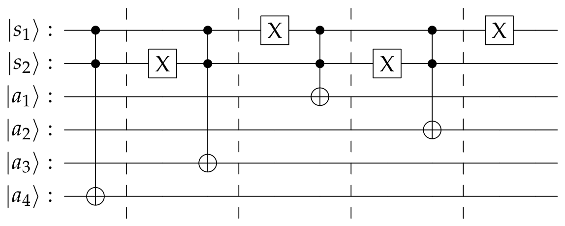
Figure A2.
Circuit decomposition of the expansion operation on the all-zero component of using an ancilla qubit .
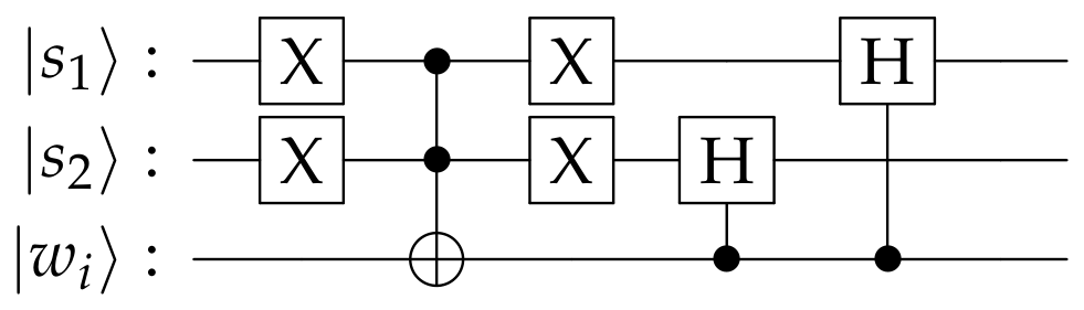
References
- Karp, R.M. Reducibility Among Combinatorial Problems. In 50 Years of Integer Programming 1958–2008: From the Early Years to the State-of-the-Art; Jünger, M., Liebling, T.M., Naddef, D., Nemhauser, G.L., Pulleyblank, W.R., Reinelt, G., Rinaldi, G., Wolsey, L.A., Eds.; Springer: Berlin/Heidelberg, Germany, 2010; pp. 219–241. [Google Scholar] [CrossRef] [Scilit]
- Paturi, R.; Pudlák, P.; Zane, F. Satisfiability Coding Lemma. In Proceedings of the 38th Annual IEEE Symposium on Foundations of Computer Science (FOCS ’97); IEEE: New York, NY, USA, 1997; pp. 566–574. [Google Scholar] [CrossRef] [Scilit]
- Schöning, U. A probabilistic algorithm for k-SAT and constraint satisfaction problems. In Proceedings of the 40th Annual IEEE Symposium on Foundations of Computer Science (FOCS ’99); IEEE: New York, NY, USA, 1999; pp. 410–414. [Google Scholar] [CrossRef] [Scilit]
- Brueggemann, T.; Kern, W. An improved deterministic local search algorithm for 3-SAT. Theor. Comput. Sci. 2004, 329, 303–313. [Google Scholar] [CrossRef] [Scilit]
- Hofmeister, T.; Schöning, U.; Schuler, R.; Watanabe, O. A Probabilistic 3—SAT Algorithm Further Improved. In STACS 2002, Proceedings of the 19th Annual Symposium on Theoretical Aspects of Computer Science, Antibes–Juan les Pins, France, 14–16 March 2002; Springer: Berlin/Heidelberg, Germany, 2002; pp. 192–202. [Google Scholar] [CrossRef] [Scilit]
- Paturi, R.; Pudlák, P.; Saks, M.E.; Zane, F. An improved exponential-time algorithm for k-SAT. J. ACM 2005, 52, 337–364. [Google Scholar] [CrossRef] [Scilit]
- Hertli, T. 3-SAT Faster and Simpler—Unique-SAT Bounds for PPSZ Hold in General. SIAM J. Comput. 2014, 43, 718–729. [Google Scholar] [CrossRef] [Scilit]
- Hansen, T.D.; Kaplan, H.; Zamir, O.; Zwick, U. Faster k-SAT algorithms using biased-PPSZ. In Proceedings of the 51st Annual ACM SIGACT Symposium on Theory of Computing (STOC ’19), Phoenix, AZ, USA, 23–26 June 2019; pp. 578–589. [Google Scholar] [CrossRef] [Scilit]
- Dantsin, E.; Goerdt, A.; Hirsch, E.A.; Kannan, R.; Kleinberg, J.; Papadimitriou, C.; Raghavan, P.; Schöning, U. A deterministic (2 − 2/(k + 1))n algorithm for k-SAT based on local search. Theor. Comput. Sci. 2002, 289, 69–83. [Google Scholar] [CrossRef] [Scilit]
- Moser, R.A.; Scheder, D. A Full Derandomization of Schöning’s k-SAT Algorithm. In Proceedings of the 43rd Annual ACM Symposium on Theory of Computing (STOC ’11), San Jose, CA, USA, 6–8 June 2011; pp. 245–252. [Google Scholar] [CrossRef] [Scilit]
- Scheder, D. Guided Search and a Faster Deterministic Algorithm for 3-SAT. In LATIN 2008: Theoretical Informatics; Laber, E.S., Bornstein, C., Nogueira, L.T., Faria, L., Eds.; Springer: Berlin/Heidelberg, Germany, 2008; pp. 60–71. [Google Scholar] [CrossRef] [Scilit]
- Makino, K.; Tamaki, S.; Yamamoto, M. Derandomizing the HSSW Algorithm for 3-SAT. Algorithmica 2013, 67, 112–124. [Google Scholar] [CrossRef] [Scilit][Green Version]
- Shor, P.W. Polynomial-Time Algorithms for Prime Factorization and Discrete Logarithms on a Quantum Computer. SIAM J. Comput. 1997, 26, 1484–1509. [Google Scholar] [CrossRef] [Scilit]
- Grover, L.K. Quantum Mechanics Helps in Searching for a Needle in a Haystack. Phys. Rev. Lett. 1997, 79, 325–328. [Google Scholar] [CrossRef] [Scilit]
- Shenvi, N.; Kempe, J.; Whaley, K.B. Quantum random-walk search algorithm. Phys. Rev. A 2003, 67, 052307. [Google Scholar] [CrossRef] [Scilit]
- Schuld, M.; Sinayskiy, I.; Petruccione, F. An introduction to quantum machine learning. Contemp. Phys. 2015, 56, 172–185. [Google Scholar] [CrossRef] [Scilit]
- Biamonte, J.; Wittek, P.; Pancotti, N.; Rebentrost, P.; Wiebe, N.; Lloyd, S. Quantum machine learning. Nature 2017, 549, 195–202. [Google Scholar] [CrossRef] [Scilit]
- Gemeinhardt, F.; Garmendia, A.; Wimmer, M.; Weder, B.; Leymann, F. Quantum Combinatorial Optimization in the NISQ Era: A Systematic Mapping Study. ACM Comput. Surv. 2024, 56, 1–36. [Google Scholar] [CrossRef] [Scilit]
- Ge, X.; Wu, R.B.; Rabitz, H. The optimization landscape of hybrid quantum-classical algorithms: From quantum control to NISQ applications. Annu. Rev. Control 2022, 54, 314–323. [Google Scholar] [CrossRef] [Scilit]
- Nardin, A.; D’Andreagiovanni, F. A Quantum-Inspired Ant Colony Optimization Algorithm for Parking Lot Rental to Shared E-Scooter Services. Algorithms 2024, 17, 80. [Google Scholar] [CrossRef] [Scilit]
- Jiang, J.R.; Wang, Y.J. Using a Simplified Quantum Counter to Implement Quantum Circuits Based on Grover’s Algorithm to Tackle the Exact Cover Problem. Mathematics 2025, 13, 90. [Google Scholar] [CrossRef] [Scilit]
- Jiang, J.R. Dicke State Quantum Search for Solving the Vertex Cover Problem. Mathematics 2025, 13, 3005. [Google Scholar] [CrossRef] [Scilit]
- Mikes, C.; Gutman, D.H.; Howle, V.E. Quantum-Enhanced Generalized Pattern Search Optimization. Quantum Rep. 2024, 6, 509–521. [Google Scholar] [CrossRef] [Scilit]
- Ablayev, F.; Salikhova, N.; Ablayev, M. Hybrid Classical–Quantum Text Search Based on Hashing. Mathematics 2024, 12, 1858. [Google Scholar] [CrossRef] [Scilit]
- Pratibha; Mahmud, N. A Reconfigurable Framework for Hybrid Quantum–Classical Computing. Algorithms 2025, 18, 271. [Google Scholar] [CrossRef] [Scilit]
- Dunjko, V.; Ge, Y.; Cirac, J.I. Computational Speedups Using Small Quantum Devices. Phys. Rev. Lett. 2018, 121, 250501. [Google Scholar] [CrossRef] [Scilit]
- Ambainis, A. Quantum search algorithms. ACM SIGACT News 2004, 35, 22–35. [Google Scholar] [CrossRef] [Scilit]
- Brassard, G.; Høyer, P.; Mosca, M.; Tapp, A. Quantum amplitude amplification and estimation. In Quantum Computation and Information; Contemporary Mathematics; American Mathematical Society: Providence, RI, USA, 2002; Volume 305, pp. 53–74. [Google Scholar] [CrossRef] [Scilit]
- Brehm, M.; Weggemans, J. Assessing fault-tolerant quantum advantage for k-SAT with structure. Quantum 2026, 10, 1975. [Google Scholar] [CrossRef] [Scilit]
- Abbas, A.; Ambainis, A.; Augustino, B.; Bärtschi, A.; Buhrman, H.; Coffrin, C.; Cortiana, G.; Dunjko, V.; Egger, D.J.; Elmegreen, B.G.; et al. Challenges and opportunities in quantum optimization. Nat. Rev. Phys. 2024, 6, 718–735. [Google Scholar] [CrossRef] [Scilit]
- Zhang, Y.; Lewalle, P.; Whaley, K.B. Solving k–SAT problems with generalized quantum measurement. npj Quantum Inf. 2025, 11, 170. [Google Scholar] [CrossRef] [Scilit]
- Liu, L.; Qian, L.; Wu, X.Y.; Fan, C.R.; Zhang, L.F.; Cai, D.B.; Lu, H.J.; Wang, T.J.; Wang, C. Solving vehicle routing problem using Grover adaptive search algorithm. IEEE Trans. Intell. Transp. Syst. 2025, 26, 9682–9692. [Google Scholar] [CrossRef] [Scilit]
- Lu, Q.; Wei, S.; Zeng, J.; Yang, W.; Zheng, M.; Chang, P.; Ruan, D.; Wang, Z.; Long, G. Space-efficient quantum solvers for Boolean satisfiability problems via structural reduction. Phys. Rev. A 2026. accepted. [Google Scholar] [CrossRef] [Scilit]
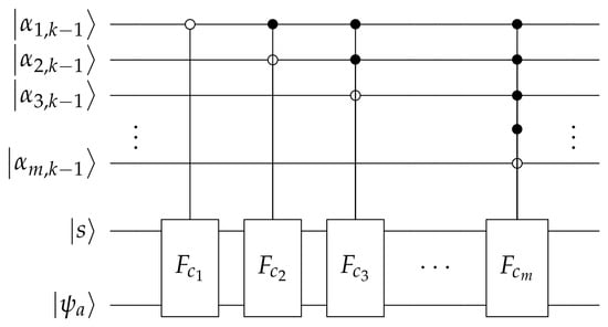
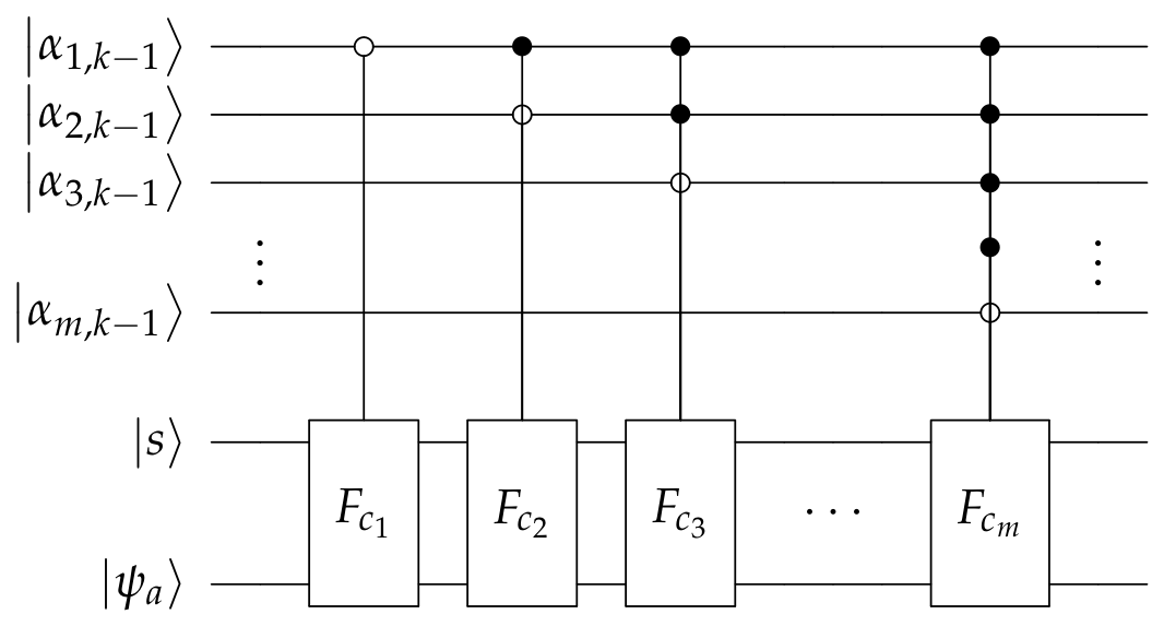
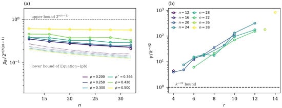
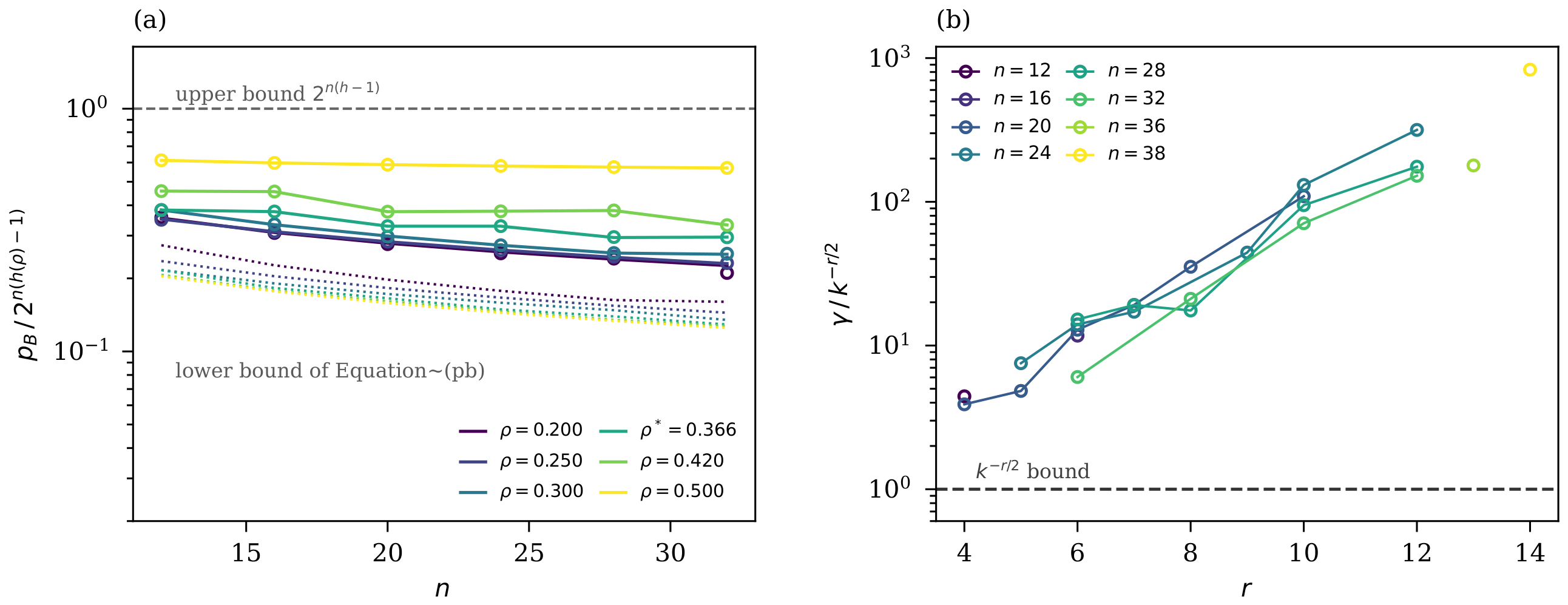
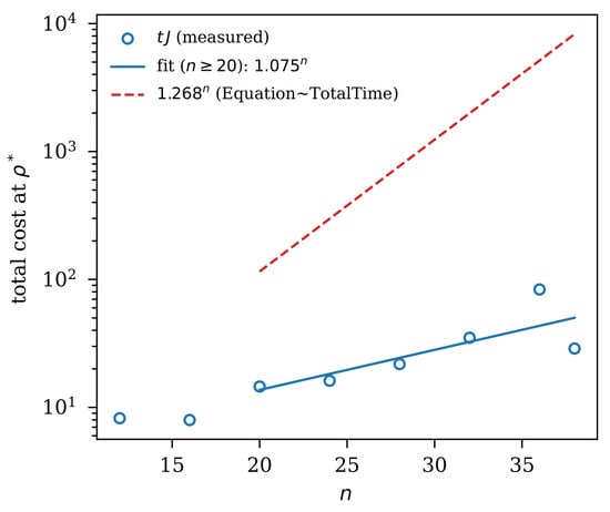
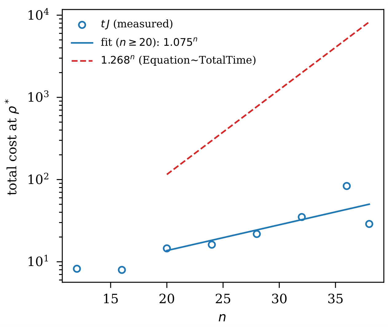
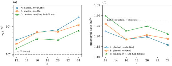

Disclaimer/Publisher’s Note: The statements, opinions and data contained in all publications are solely those of the individual author(s) and contributor(s) and not of MDPI and/or the editor(s). MDPI and/or the editor(s) disclaim responsibility for any injury to people or property resulting from any ideas, methods, instructions or products referred to in the content. |
© 2026 by the author. Licensee MDPI, Basel, Switzerland. This article is an open access article distributed under the terms and conditions of the Creative Commons Attribution (CC BY) license.