Target-Adaptive CAN Intrusion Detection Across Heterogeneous Vehicle Datasets via Robust Residual Modeling and Empirical Block-Rank Calibration

Abstract

Vehicle-specific CAN identifiers, timing, and payload encodings complicate intrusion detection across vehicles. This study proposes a 12-dimensional residual representation that measures deviations from each vehicle’s normal communication and combines it with Isolation Forest (IF) and empirical block-rank (EBR) calibration. The method uses normal-only target adaptation: trusted target-normal commissioning data define the residual references, fit the detector, and calibrate block-level alarms. Across four can-train-and-test scenarios with five random seeds each, the mean area under the receiver operating characteristic curve (AUROC) was 0.918, the area under the precision–recall curve (AUPRC) was 0.622, and the Matthews correlation coefficient (MCC) was 0.573. Capture-disjoint and leave-one-capture-out AUPRC values decreased to 0.553 and 0.521. At α = 0.05, the block false-positive rate (FPR) was 0.072, and the attack-block recall was 0.786; the pooled false-alarm event rate after event aggregation was 11.1 per hour. Repeating the commissioning procedure on ROAD with newly fitted target-specific models achieved an AUPRC of 0.503, with split-level recall ranging from 0 to 0.571. Matched comparisons showed the contribution of the residual representation, while capture-separated and ROAD results identified commissioning coverage and alarm stability as central operational challenges.

1. Introduction

Modern vehicles depend on continuous communication among electronic control units (ECUs) for powertrain, chassis, body, and advanced driver-assistance functions. Controller Area Network (CAN) remains widely used because of its low cost, priority-based arbitration, reliability, and mature automotive ecosystem [1]. However, CAN was designed for a trusted in-vehicle environment and does not natively provide sender authentication or payload confidentiality. An adversary who gains access through a diagnostic interface, telematics or infotainment system, compromised ECU, or exposed gateway can inject, replay, suppress, or modify syntactically valid frames [2,3,4]. Anomaly-based intrusion detection is therefore attractive for legacy and heterogeneous platforms because it can monitor raw communication without redesigning the underlying protocol.

Existing CAN intrusion detection systems (IDSs) exploit complementary forms of evidence. Timing and frequency methods model periodicity, inter-arrival behavior, message counts, and transmission gaps [5,6,7], with related temporal formulations extending these cues [8,9,10]. Payload- and signal-aware methods capture manipulations that preserve nominal transmission rates [11,12,13]. Recent studies include signal-level deep models, multimodal and ensemble fusion [14,15,16], knowledge and graph representations [17,18], lightweight image or graph encodings [19,20], and adaptive, multi-knowledge, and physical-layer designs [21,22,23]. Ensemble learning combines complementary predictors through bagging of resampled learners, sequential boosting, voting over base predictions, or stacking with a learned second-level model. Interpretable ensemble applications in rockburst risk assessment [24], material-strength prediction [25], and wave-height prediction [26] provide related examples of combining predictive diversity with explanations of model output.

Vehicle heterogeneity complicates these approaches because identifier assignments, timing scales, payload encodings, and transition structures change with vehicle configuration. The can-train-and-test and ROAD datasets support evaluation across vehicles, attack families, and collection conditions [27,28], while studies of capture design show that the evaluation protocol affects measured performance [29,30]. Evaluation must distinguish gains from target-normal data access, feature representation, and estimator choice and connect anomaly ranking with operational alarms under serially dependent traffic. These requirements define the gap addressed by this study.

Operational alarm calibration connects anomaly scores to detection decisions. Recent CAN IDS studies emphasize discrimination under benchmark-specific thresholds [31,32,33]. Conformal ranking provides a finite-sample interpretation under exchangeability, whereas serial dependence and distribution shift require additional assumptions or adaptive procedures [34,35,36]. In CAN streams, the testing unit and temporal aggregation determine how a nominal alarm level relates to realized false alarms. Evaluating window, block, and event decisions therefore connects score discrimination with the practical alarm burden.

This study addresses these requirements through a normal-only target-adaptation framework. For each vehicle, trusted normal commissioning traffic defines local residual references, fits an anomaly detector, and supplies a separate calibration partition. Target adaptation denotes this vehicle-specific fitting procedure; workflow replication repeats it on another dataset with newly fitted target-specific models. The protocol augments the official can-train-and-test unknown-vehicle setting with target-normal commissioning data. Source-only and source-supported behavioral models provide comparison baselines.

The proposed contribution is a 12-dimensional target-normal residual representation integrated with dependence-informed block calibration. The vector combines payload and timing deviations with identifier rarity, novelty, transition surprise, and distributional change. The calibration workflow estimates a temporal scale from normal scores, constrains block length to preserve empirical rank resolution, and compares test-block maxima with calibration maxima. Isolation Forest and empirical ranking supply the established estimator and rank rule. Matched inputs, estimator comparisons, and feature ablations examine the representation’s contribution, while capture separation, contamination, and operational sensitivity analyses test the commissioning and alarm workflow.

2. Materials and Methods

2.1. Problem Formulation and Overall Framework

The framework converts trusted normal CAN traffic into block-level intrusion alarms in four stages. Adaptation data first define the residual references for each analysis window. Isolation Forest then maps residual vectors to anomaly scores. The autocorrelation of normal scores proposes a block length, which is constrained by the available calibration data; EBR compares each test-block maximum with the calibration maxima. Finally, a merge horizon and refractory interval combine positive blocks into alarm events. Behavioral-role features support vehicle-configuration diagnostics and comparison baselines.

Let the chronologically ordered CAN stream from vehicle $v$ be ${\mathcal{M}}^v=\{n_v^m{n=1}_N^{\}}$, where each frame contains timestamp $n_v^t$, CAN identifier $n_v^i$, data length $n_v^d$, and payload vector $n_v^x$. The frame representation is

$$n_v^m=\left(n_v^t,n_v^i,n_v^d,n_v^x\right)$$

(1)

The detector models the target vehicle’s normal communication and flags deviations through one-class anomaly scoring. Adaptation data estimate the residual references and robust standardization, fit the detector, and characterize temporal dependence. A disjoint normal calibration partition determines the alarm rule. Feature design, model fitting, and threshold selection use normal traffic in the clean protocol; attack-family labels enter only evaluation and the separately defined contamination experiment. Source-based baselines are fitted on normal source frames.

Commissioning assumes trusted, attack-free normal traffic. In can-train-and-test, benchmark labels identify the prefix preceding the first attack; dedicated ROAD ambient files supply normal data for that dataset. The partition rules are specified in Section 2.4. Field commissioning would obtain trusted traffic through controlled manufacturing or service-center collection, supported by data-sanitization checks. Section 3.5 evaluates sensitivity to contamination of the normal reference and calibration data.

Frames were segmented into non-overlapping fixed-duration windows $W_q$ of length $\Delta T=0.05\hspace{0.17em}\mathrm{s}$, and windows with fewer than $n_{min}=8$ frames were discarded. Alarm calibration used the separate normal partition $t_c^D$.

2.2. Behavioral Diagnostics and Target-Normal Residual Scoring

The same numerical CAN identifier need not represent the same function across vehicles. Each identifier $i$ was therefore characterized by an eight-dimensional normal-traffic signature comprising transmission frequency $f_i$, median same-ID inter-arrival time ${\tilde{\Delta }}_i$, coefficient of variation ${CV}_i$, normalized payload entropy $H_i$, bit-flip rate $B_i$, transition entropy $i_{tr}^H$, and normalized transition-graph in- and out-degrees $i_{in}^d$ and $i_{out}^d$:

$$i_v^s=\left[log\left(1+f_i\right),{\tilde{\Delta }}_i,{CV}_i,H_i,B_i,i_{tr}^H,i_{in}^d,i_{out}^d\right]$$

(2)

Because absolute signature values remain vehicle-dependent, each dimension was converted to a within-vehicle rank. For signature dimension $k$, the resulting role coordinate is

$${i,k}_v^r={\displaystyle \frac{{rank}_v\left({i,k}_v^s\right)-0.5}{\left|I^v\right|}}$$

(3)

For each window $W_q$, the behavioral representation aggregates frame-level role vectors using the component-wise mean, 90th percentile, and standard deviation, together with the fraction of reference identifiers active in the window. With ${i_n}_v^r$ denoting the role vector of frame $n$ and $I_q$ denoting the active identifier set, the window representation is

$$h^v\left(W_q\right)=\left[mean\left({i_n}_v^r\right),Q_{0.9}\left({i_n}_v^r\right),std\left({i_n}_v^r\right),\left|I_q\right|/\left|I^v\right|\right]$$

(4)

Behavioral normalization can improve comparability while attenuating sparse local deviations. A separate target-local reference was therefore constructed using only $t_a^D$. For payload byte $b$ of identifier $i$, the normal center and scale were estimated by the median and median absolute deviation (MAD), with a floor ${\sigma }_{min}$ for nearly constant bytes:

$${\mu }_{i,b}=median\left(x_{i,b}\right), {\sigma }_{i,b}=max\{1.4826\hspace{0.17em}MAD\left(x_{i,b}\right),{\sigma }_{min}\}$$

(5)

Frame-level payload and inter-arrival residuals were defined by robust standardized deviations. The empirical target-normal identifier probability ${\pi }_i$ and transition probability $P\left(i\to j\right)$ additionally defined identifier- and transition-surprise terms. Residual magnitudes were clipped at 12; identifiers absent from $t_a^D$ received a fixed penalty of 8; the bottom 20% of positive target-normal identifier probabilities defined the rare-ID set. For frame $n$, the principal residual quantities are

$$\begin{gathered} {n,b}_x^z={\displaystyle \frac{\left|x_{n,b}-{i_n,b}_x^{\mu }\right|}{{i_n,b}_x^s}}, n_{\Delta }^z={\displaystyle \frac{\left|\Delta t_n-{i_n}_{\Delta }^{\mu }\right|}{{i_n}_{\Delta }^s}}. \\ {n}_{id}^u=-log{\pi }_{i_n}, n_{tr}^u=-logP\left(i_{n-1}\to i_n\right). \end{gathered}$$

(6)

Payload centers and scales were estimated from each identifier’s bytes using Equation (5); timing centers and scales used the analogous median and MAD rule for same-identifier inter-arrival times. Zero-probability identifier and transition events received the fixed unseen-event penalty before logarithmic scoring. Scale floors, smoothing, payload-byte aggregation, and capture-boundary handling were held fixed across experiments.

Aggregating frame residuals and identifier-use statistics yields the twelve-dimensional vector below. Its total-variation term compares the window identifier distribution $q_q$ with the target-normal distribution $\pi$:

$$\begin{gathered} g_q=\left[q_{unseen}^u,q_{rare}^u,q_x^{\psi },q_{\Delta }^{\psi },q_{tr}^{\psi },q_{id}^{\psi },D_{TV}\left(q_q,\pi \right)\right]. \\ {q}_x^{\psi }=\left[mean\left(z^{x,mean}\right),Q_{0.9}\left(z^{x,max}\right),max\left(z^{x,max}\right)\right]. \\ {q}_{\Delta }^{\psi }=\left[mean\left(z^{\Delta }\right),Q_{0.9}\left(z^{\Delta }\right)\right], q_{tr}^{\psi }=\left[mean\left(u^{tr}\right),Q_{0.9}\left(u^{tr}\right)\right], q_{id}^{\psi }=\left[mean\left(u^{id}\right),Q_{0.9}\left(u^{id}\right)\right]. \end{gathered}$$

(7)

In Equation (7), dimensions 1–2 are the unseen-ID and rare-ID ratios; 3–5 are mean, upper-quantile, and maximum payload deviations; 6–7 are mean and upper-quantile timing deviations; 8–9 are mean and upper-quantile transition surprise; 10–11 are mean and upper-quantile identifier surprise; 12 is the identifier-distribution total variation. Payload and timing residuals measure byte and transmission changes, while the remaining terms measure unusual identifier use and sequencing. Means retain sustained deviations, and upper-quantile and maximum summaries retain sparse excursions. All references are estimated from adaptation data and held fixed during evaluation. These decoder-free statistics are evaluated through feature-group ablations in Section 3.3.

Isolation Forest was fitted to target-adaptation residual vectors using 100 trees and at most 256 observations per learner. Each feature was standardized with its adaptation-set median and MAD (Equation (8)), and the forest’s anomaly score was passed to calibration. The behavioral IF baseline combined source and target-adaptation windows at a 1:4 ratio. One-class support vector machine (OCSVM) and local outlier factor (LOF) baselines used the same standardized behavioral inputs.

Estimator comparisons shared the adaptation and calibration data, evaluation windows, and block construction. Table 1 compares IF, OCSVM, and LOF on behavioral inputs; Section 3.3 compares them on identical standardized residual inputs and compares raw with residual features under IF. Neural baselines used target-normal adaptation data and returned one score per evaluation window for the common block-decision layer. Source-only baselines used their separately specified data access. Table 1 summarizes the pipeline settings.

Table 1. Prespecified analysis parameters common to the can-train-and-test and ROAD experiments.

Setting	Parameter	Prespecified Value
Window construction	Duration; minimum frames	0.05 s; 8 frames
Residual scoring	Magnitude clip; unseen-event penalty	12; 8
Rare-identifier rule	Positive-probability cutoff	Bottom 20%
Isolation Forest	Trees; maximum observations per learner	100; 256
Behavioral baseline	Source-to-target window ratio	1:4
ACF search	Initial lags; extension; maximum; in-band run	80; 40; 240; 8 lags
Rank resolution	Minimum calibration blocks	100
Alarm levels	Evaluated α; default α	{0.01, 0.025, 0.05, 0.075, 0.10}; 0.05
Target-normal split	Oracle-clean prefix reserved; adaptation/calibration	First 40% of clean prefix; adaptation/calibration: 20%/20% of full prefix
Repeated fits	Isolation Forest seeds per scenario	5
Event post-processing	Merge horizon; refractory interval	10 s; 30 s

The multilayer perceptron autoencoder (MLP-AE) used a symmetric 12-32-8-32-12 encoder–decoder with rectified linear unit (ReLU) hidden units and a linear output. The long short-term memory autoencoder (LSTM-AE) processed sequences of 16 residual windows with encoder widths of 64 and 32, a mirrored decoder, and dropout of 0.20. Deep support vector data description (Deep SVDD) used a bias-free 12-32-16-8 embedding and a one-class center objective. The temporal convolutional network autoencoder (TCN-AE) used 16-window sequences; three causal residual blocks with 32, 64, and 64 channels; a kernel size of 3; dilations of 1, 2, and 4; and a 16-dimensional latent code. The autoencoders used mean squared reconstruction errors, Adam with a learning rate of 0.001, a batch size of 64, a maximum of 100 epochs, and early stopping with a patience of 10 epochs. Deep SVDD used Adam with a learning rate of 0.0001, a batch size of 128, and 150 epochs. Reconstruction error or squared distance from the Deep SVDD center defined the window score. Hyperparameters followed representative normal-only CAN and time-series designs [37,38,39] and remained fixed across scenarios.

$${\tilde{g}}_{q,j}={\displaystyle \frac{g_{q,j}-median\left(j_a^G\right)}{1.4826\hspace{0.17em}MAD\left(j_a^G\right)+\epsilon }}, a_q=F^R\left({\tilde{g}}_q\right).$$

(8)

The hybrid analysis tested whether behavioral scores added information to residual scores. Both scores were standardized using target-normal adaptation scores and combined by a predefined maximum rule. All estimator comparisons used the block length selected from the primary residual score, keeping the decision unit common across methods.

2.3. Dependence-Informed Empirical Block-Rank Calibration

Consecutive CAN windows can remain dependent even when they do not overlap. The sample autocorrelation function (ACF) of target-residual adaptation scores was therefore estimated within capture boundaries. Starting from 80 lags, the inspected range was extended in steps of 40 up to 240 lags whenever the current tail remained unresolved. The candidate length was the first lag of a run of eight consecutive autocorrelations falling within the approximate 95% sampling band; if no such run was observed, the candidate was set immediately after the last significant lag within the inspected range. Because an excessively large block would reduce empirical rank resolution, the operational length was further constrained to retain at least 100 normal calibration blocks whenever feasible:

$$\begin{gathered} b=min\left(b_{ACF},b_{res}\right). \\ {b}_{res}=max\left\{b^{\prime }:\sum _{f}floor\left({\displaystyle \frac{f_c^N}{b^{\prime }}}\right)\ge M_{min}\right\} \end{gathered}$$

(9)

Capture-specific calibration-window counts determine the largest block length that retains at least 100 calibration maxima. Equation (9) constrains the ACF candidate to this length. The 100-block minimum supports empirical rank resolution near the lowest evaluated alarm level, α = 0.01. Calibration scores were partitioned into non-overlapping blocks within capture boundaries, and each block was represented by its maximum anomaly score. For calibration block j,

$$A_j=\underset{q\in B_j}{max}{a}_q.$$

(10)

For a test block with maximum score S*, Equation (11) defines a smoothed upper-tail empirical rank statistic by counting calibration-block maxima at least as large as S*. A block is declared positive when that statistic does not exceed α:

$$p^{test}={\displaystyle \frac{1+{\displaystyle {\sum }_{j=1}^M}1\left(A_j\ge A^{test}\right)}{M+1}}, \widehat{y}=1\left(p^{test}\le \alpha \right).$$

(11)

At the default α = 0.05, Equation (11) supplies the empirical upper-tail rank used for block decisions. Its finite-sample conformal interpretation requires block exchangeability. Realized FPR and recall assess calibration under the remaining temporal dependence and operating-condition changes.

Evaluation used non-overlapping test blocks of operational length b. A block was positive if any constituent window overlapped a labeled attack interval; blocks containing only benign windows formed the FPR denominator. Blocks remained within capture boundaries, and incomplete terminal blocks were discarded. AUROC and AUPRC used the block-maximum score. MCC, FPR, and recall used the default α = 0.05 decisions. MCC was computed from block-level TP, FP, TN, and FN counts, with a zero denominator assigned a value of 0. Window-rule decisions were mapped to the same reporting blocks through an any-window rule.

Window Percentile applied the empirical 1 − α quantile of calibration-window scores to individual test windows and mapped the resulting decisions to a block alarm using an any-window rule. Window empirical rank (Window ER) replaced the percentile threshold with the same upper-tail rank construction at the window level and used the same any-window mapping. Bonferroni empirical rank (Bonferroni ER) tested each constituent window at α/b before applying the any-window rule. ACF-Block Percentile applied an empirical 1 − α quantile to calibration-block maxima, whereas EBR applied Equation (11) directly to the test-block maximum. These rules share the same anomaly score but not the same primitive testing unit; comparisons involving window rules therefore combine within-block multiplicity with temporal and distributional dependence.

2.4. Experimental Protocols and Performance Measures

Primary evaluation used the unknown-vehicle/unknown-attack subset (test_04_unknown_vehicle_unknown_attack) of each of the four official can-train-and-test sets [27], augmented with target-normal commissioning data. The source/target scenarios were Chevrolet Impala/Chevrolet Silverado, Chevrolet Traverse/Subaru Forester, Chevrolet Silverado/Subaru Forester, and Subaru Forester/Chevrolet Traverse. Source-based baselines used source frames after labeled attacks were removed. Five random seeds varied source subsampling and Isolation Forest construction.

For each target capture, labels delimited the clean prefix preceding the first attack. The first 40% of its frames, rounded down to an integer count, formed the commissioning set. Adaptation received the first half of that set, again rounded down, and calibration received the remainder. The remaining 60% of the clean prefix and the subsequent stream formed the chronological evaluation set. Windows, transition histories, recurrent sequences, and decision blocks were constructed separately within each partition and capture, with histories reset at boundaries. Adaptation supplied feature references, standardization, detector fitting, and score autocorrelation; calibration supplied block maxima and the counts used in Equation (9).

ROAD repeated the feature definitions, detector settings, block-maximum scoring, and alarm levels with new references and detectors fitted to ROAD normal traffic [28]. Each of the five seeded file splits assigned five dynamometer ambient files to adaptation, two to calibration, and three to benign testing (Table A1), keeping file roles disjoint within a split. Attack files supplied the attack evaluation. Two highway/street ambient files supplied the road-driving stress condition, and four accelerator post-exploit captures were profiled separately. Block length followed Section 2.3: ROAD adaptation scores supplied the ACF candidate, and calibration-window counts supplied the rank-resolution constraint in Equation (9). All five splits used an operational length of 48 windows (2.4 s), retaining 211–796 calibration blocks (Table A1). The splits reuse ambient and attack captures, providing overlapping resamples on one vehicle.

AUROC and AUPRC assess ranking of block-maximum scores. Can-train-and-test AUPRC lift divides AUPRC by scenario-specific attack-block prevalence. Seeds were averaged within each scenario before calculating the mean and sample standard deviation (SD) across the four can-train-and-test scenarios. ROAD reports the mean and sample SD across five file splits; Table A2 gives the individual confusion matrices.

Detection latency was measured from the first attack-labeled frame to the completion of the first newly alarm-raising decision unit for which its completion time fell within the labeled attack interval. The decision unit was a window for window rules and a block for block rules. Scenario latency was the median across captures with a qualifying detection; captures without one were excluded from this conditional latency summary. An alarm that was already active at attack onset did not qualify as a new detection. Block-level metrics retained the overlap labels in Section 2.3. Every attack-labeled block entered the recall denominator, with an unalarmed attack block counted as a false negative. An alarmed block was a true positive if any constituent window overlapped a labeled attack interval and a false positive if all constituent windows were benign. These labels also applied to blocks that were completed after the attack ended.

Capture-disjoint evaluation assigned separate captures to adaptation, calibration, and testing, using label-verified clean prefixes for commissioning (Table A3). In leave-one-capture-out (LOCO) evaluations, each member of the scenario-specific pool was held out once for testing. Every remaining capture followed the primary chronological commissioning rule: With N denoting the label-verified benign frames of that capture before the first attack, the first n = ⌊0.40 × N⌋ frames entered commissioning, of which the first ⌊0.50 × n⌋ frames were assigned to adaptation, and the remaining n − ⌊0.50 × n⌋ frames were assigned to calibration. The held-out capture contributed evaluation frames only. Capture and partition boundaries separated windows, transition histories, recurrent sequences, and decision blocks, with histories reset at each boundary. Held-out predictions were aggregated within each scenario before calculating the four-scenario summary. These protocols assess recording conditions beyond the primary chronological holdout.

Commissioning contamination was introduced by replacing randomly selected normal analysis windows with an equal number of target windows overlapping labeled attacks. Replaced windows were treated as nominal during reference estimation, fitting, or calibration, and partition sizes remained fixed. The joint-contamination sweep used 0%, 1%, 3%, 5%, and 10%; the 5% location analysis contaminated adaptation only, calibration only, or both. Contamination windows were excluded from final evaluation blocks. Attack labels selected the substitutions for this controlled experiment.

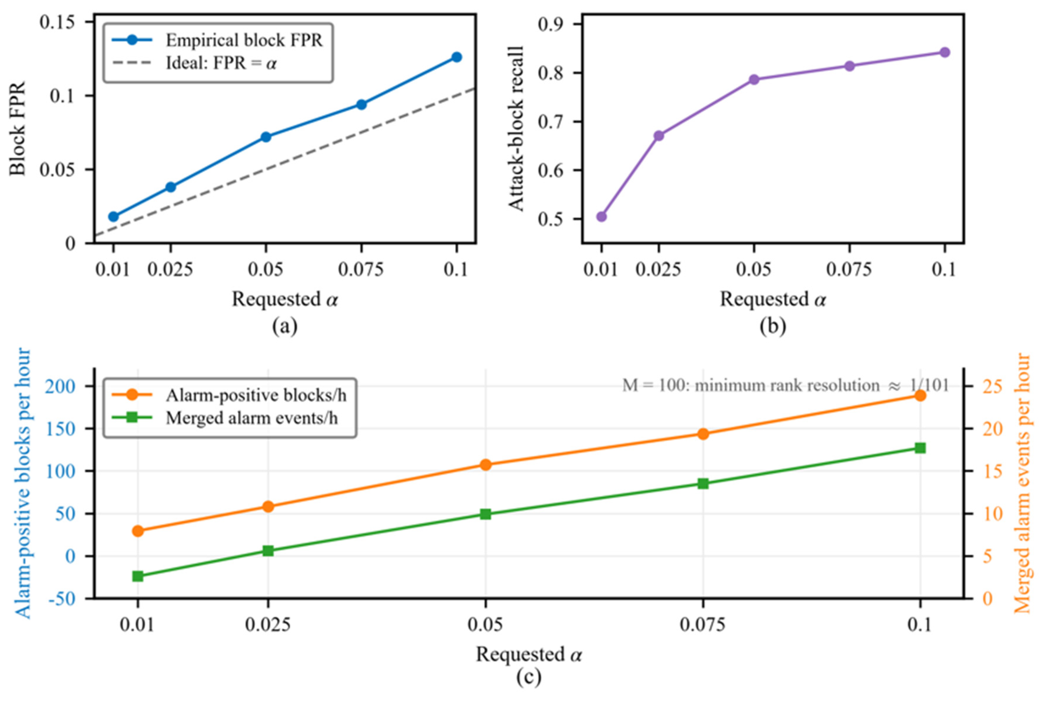
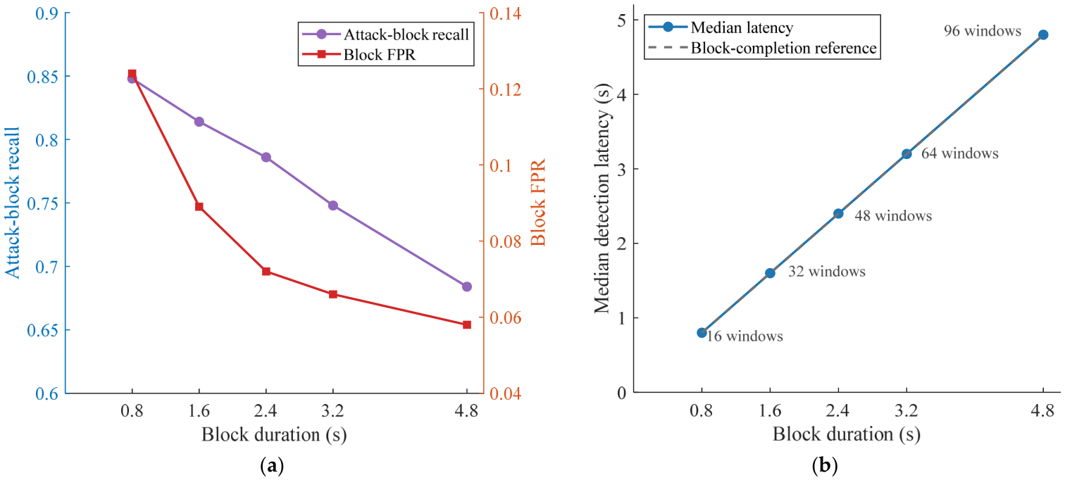
Operating-level analysis used α ∈ {0.01, 0.025, 0.05, 0.075, 0.10}. With 100 calibration blocks, the minimum smoothed rank is 1/101 ≈ 0.0099. At α = 0.05, event processing compared no merging with merge/refractory settings of 5/15 s, 10/30 s, and 20/60 s. Block-length sensitivity used 16, 32, 48, 64, and 96 windows, corresponding to 0.8, 1.6, 2.4, 3.2, and 4.8 s. These grids provide retrospective operating-point comparisons.

3. Results

3.1. Target-Adaptive Detection and Representation Diagnostics

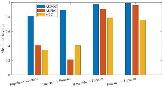
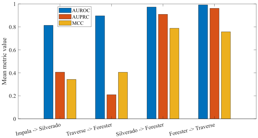
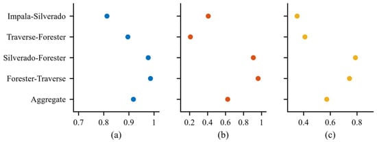
Across four can-train-and-test scenarios, the residual IF achieved an AUROC of 0.918 (SD 0.081), AUPRC of 0.622 (SD 0.372), AUPRC lift of 7.805 (SD 2.962), and MCC of 0.573 (SD 0.232). Scenario AUPRC ranged from 0.210 to 0.962, and attack-block prevalence ranged from approximately 0.027 to 0.251 (Figure 1).

Figure 1. Scenario-level target-adaptive performance of the primary target-residual IF on can-train-and-test scenarios: AUROC, AUPRC, and MCC across the four official source/target vehicle scenarios.

Silverado/Forester achieved an AUROC of 0.977, AUPRC of 0.909, and MCC of 0.788; Forester/Traverse achieved 0.986, 0.962, and 0.743, respectively. Traverse/Forester retained an AUROC of 0.896 but had an AUPRC of 0.210. The two Forester-target scenarios thus differed substantially despite sharing the target model name. Table 2 compares the estimators and decision rules.

Table 2. Target-adaptive anomaly-scoring performance and descriptive block-level decisions on can-train-and-test scenarios. Anomaly-scoring metrics are the mean (SD) across four vehicle scenarios; decision metrics are evaluated at α = 0.05. (Bold rows denote the column headers of the table’s two panels; no data values are bolded.)

Representation and Anomaly-Scoring Performance
Method	AUROC	AUPRC	AUPRC Lift	MCC
Raw source IF	0.567 (0.140)	0.248 (0.239)	2.928 (2.047)	0.158 (0.218)
Behavioral-role source IF	0.498 (0.120)	0.161 (0.131)	1.773 (0.479)	0.109 (0.077)
Target-adapted role IF	0.854 (0.056)	0.456 (0.331)	5.292 (2.112)	0.438 (0.212)
Target-adapted role OCSVM	0.857 (0.063)	0.492 (0.330)	6.214 (3.097)	0.427 (0.253)
Target-adapted role LOF	0.585 (0.105)	0.202 (0.255)	1.761 (0.689)	0.079 (0.180)
Target residual IF (primary)	0.918 (0.081)	0.622 (0.372)	7.805 (2.962)	0.573 (0.232)
Hybrid role + residual sensitivity	0.915 (0.087)	0.561 (0.407)	6.446 (2.471)	0.543 (0.246)
Descriptive Block-Level Decision Comparison at the Default Operating Point
Decision Rule	Block FPR at α = 0.05	Attack-Block Recall	Interpretation
Window Percentile	0.668	0.981	Window threshold mapped to any-window block alarm
Window ER	0.665	0.981	Window empirical rank mapped to any-window block alarm
Bonferroni ER	0.053	0.605	Within-block multiplicity correction
ACF-Block Percentile	0.080	0.794	Empirical threshold for block maxima
EBR	0.072	0.786	Empirical ranking of block maxima; descriptive under unresolved dependence

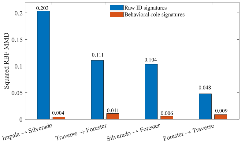
Residual IF had the highest mean ranking performance and default-threshold MCC among Table 2’s configurations. Adapted behavioral IF and OCSVM had AUPRC values of 0.456 and 0.492 compared with 0.622 for residual IF; the hybrid configuration reached 0.561. Figure 2 examines how vehicle-relative behavioral ranks changed identifier-level discrepancy.

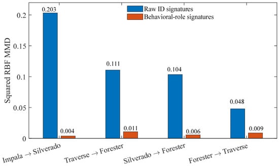
Figure 2. Identifier-level source-target representation discrepancy across four can-train-and-test scenarios: raw identifier signatures versus within-vehicle rank-normalized behavioral-role signatures.

Within-vehicle rankings reduced the standardized squared radial basis function (RBF)–kernel maximum mean discrepancy (MMD) by 81.7–98.2%, averaging 91.2% (Figure 2). Impala/Silverado decreased from 0.203 to 0.004, Silverado/Forester from 0.104 to 0.006, and Forester/Traverse from 0.048 to 0.009. Raw and role-window domain classifiers remained almost perfectly discriminative, so vehicle information persisted at the complete-window level.

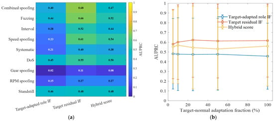
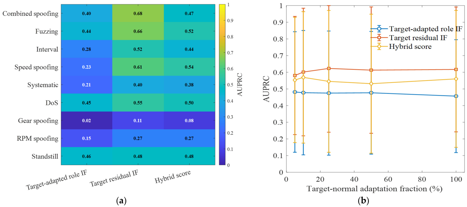
Residual IF had the highest or joint-highest mean AUPRC for each displayed attack family (Figure 3a). Relative to adapted-role IF, AUPRC increased from 0.40 to 0.68 for combined spoofing, from 0.23 to 0.61 for speed spoofing, and from 0.02 to 0.11 for gear spoofing. Gear and RPM manipulations remained the weaker families. The mean residual AUPRC changed little across adaptation fractions and reached 0.580 at the 5% budget (Figure 3b); between-scenario dispersion exceeded changes in the mean curve.

Figure 3. Attack-family AUPRC and target-normal adaptation-budget sensitivity on can-train-and-test: (a) attack-family performance; (b) target-normal adaptation-budget sensitivity.

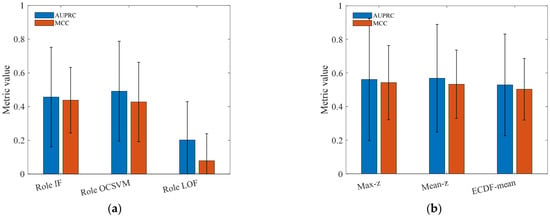
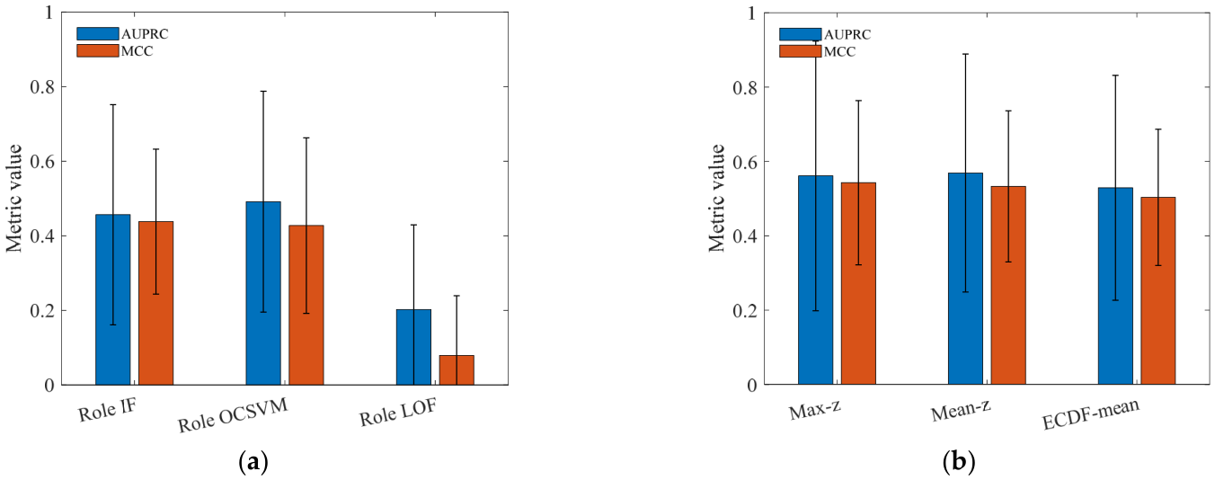
On behavioral inputs, OCSVM had a higher mean AUPRC than IF (0.492 versus 0.456), while IF had a higher MCC (0.438 versus 0.427); LOF reached an AUPRC of 0.202 and MCC of 0.079 (Figure 4a). The max-z, mean-z, and empirical cumulative distribution function (ECDF)–mean fusion rules reached an AUPRC of 0.561, 0.569, and 0.529 (Figure 4b) compared with the residual-only AUPRC of 0.622.

Figure 4. Detector and fusion sensitivity analyses: (a) adapted-role detector baselines and (b) attack-label-free fusion rules.

3.2. Block-Length Selection and Decision-Rule Comparison

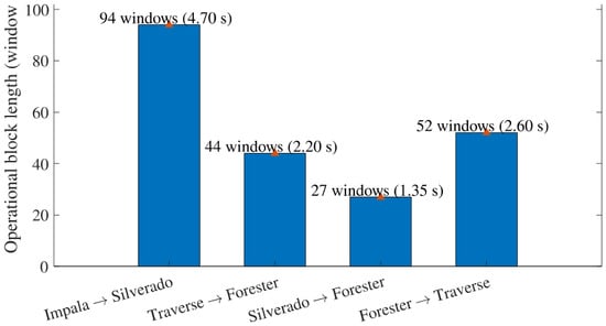
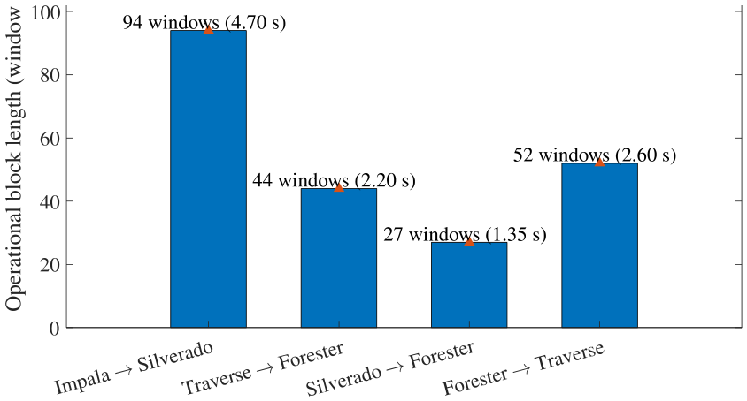
The selected block length had a median of 48 windows (2.4 s) across 20 scenario-seed runs. The rank-resolution constraint was active in all runs, and the ACF tail remained unresolved at the maximum inspected lag in 10 runs (Figure 5).

Figure 5. Resolution-constrained, dependence-informed block lengths across four can-train-and-test scenarios. Bars show operational block length in windows; labels give the corresponding duration at 0.05 s per window.

Scenario-specific lengths ranged from 27 windows (1.35 s) for Silverado/Forester to 94 windows (4.70 s) for Impala/Silverado, with intermediate lengths of 44 and 52 windows (Figure 5). Figure 6 compares the resulting decision rules at a common block-level reporting unit.

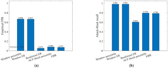
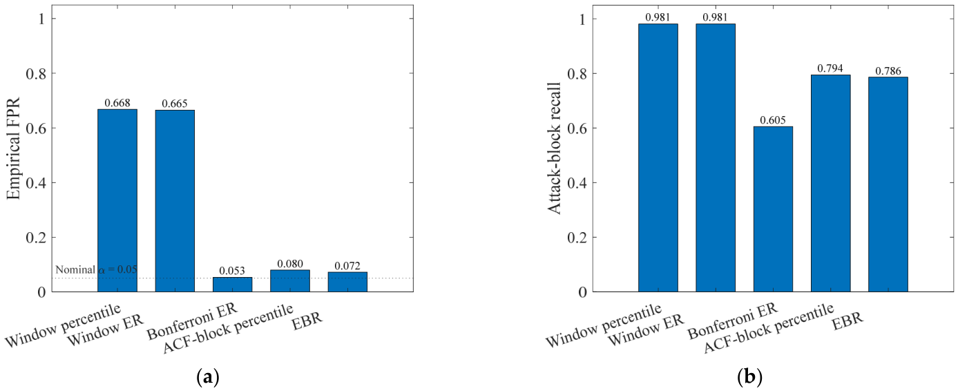
Figure 6. Descriptive can-train-and-test block-level comparison at α = 0.05: (a) empirical block FPR; (b) attack-block recall. Window rules are mapped to blocks by an any-window alarm rule.

At α = 0.05, Window Percentile and Window ER produced block FPRs of 0.668 and 0.665, with a recall of 0.981 after any-window aggregation (Figure 6). Bonferroni ER reduced FPR to 0.053, with a recall of 0.605. ACF-Block Percentile and EBR achieved FPRs of 0.080 and 0.072, with recalls of 0.794 and 0.786. The largest false-alarm reduction accompanied block-maximum calibration; the difference between the two block rules was smaller.

At the median 2.4 s block duration, an FPR of 0.072 corresponds to approximately 108 positive benign blocks per hour. The primary evaluation yielded 11.1 merged false-alarm events per hour, with 10 s merging and a 30 s refractory interval. Mean feature-construction, scoring, and calibration times were 772.7, 35.6, and 0.038 s, respectively; batch throughput was 9222 frames/s.

3.3. Matched Baselines, Feature Ablations, and Block-Level Comparison

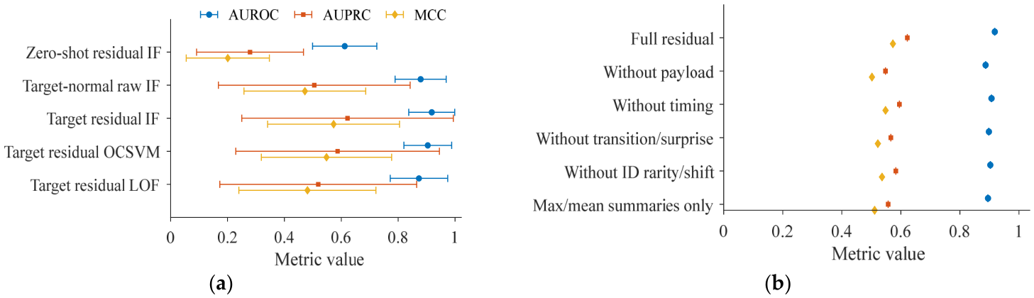
Target-normal raw-feature IF outperformed the source-normal residual baseline in Figure 7a. Under the same target-normal IF setting, residual inputs increased AUPRC from 0.505 to 0.622. IF, OCSVM, and LOF also received identical standardized residual vectors and the same calibration protocol. The IF–OCSVM AUPRC difference was 0.035, compared with the 0.117 raw-to-residual gain under IF.

Figure 7. Matched detector baselines and residual-feature ablations on can-train-and-test: (a) matched learning-setting and detector comparisons, reported as mean with SD across four scenarios; (b) residual feature-group ablations using Isolation Forest.

Residual IF exceeded target-normal raw-feature IF by 0.039 in AUROC, 0.117 in AUPRC, and 0.101 in MCC. Payload removal caused the largest AUPRC reduction of 0.074 (Figure 7b). Retaining only maximum and mean summaries reduced AUPRC by 0.065; removing transition and surprise features reduced it by 0.056; removing identifier-rarity and distribution-shift features reduced it by 0.039; removing timing features reduced it by 0.027. The full representation had the highest value on each displayed metric.

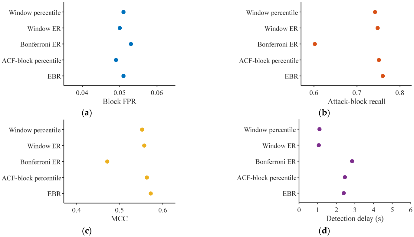
The matched-FPR analysis aligned thresholds post hoc to an evaluation-set benign block FPR near 0.05. This retrospective diagnostic compares decision rules at similar realized false-alarm levels; the primary operating point uses commissioning-based calibration. Figure 8 reports decision metrics and latency.

Figure 8. Retrospective comparison at matched evaluation-set block FPR near 0.05: (a) block FPR; (b) attack-block recall; (c) MCC; (d) median latency among detected captures, in seconds. Points represent the five decision rules, and row labels apply to both columns. Thresholds were aligned post hoc.

The five matched methods operated at a block FPR of 0.049–0.053. EBR reached a recall of 0.760 and MCC of 0.572, compared with a recall of 0.742 for Window Percentile, 0.748 for Window ER, and 0.751 for ACF-Block Percentile. Median latency was approximately 1.1 s for the two window rules, 2.4 s for EBR, and 2.85 s for Bonferroni ER (Figure 8).

3.4. Scenario Heterogeneity, Operational Burden, and ROAD Replication

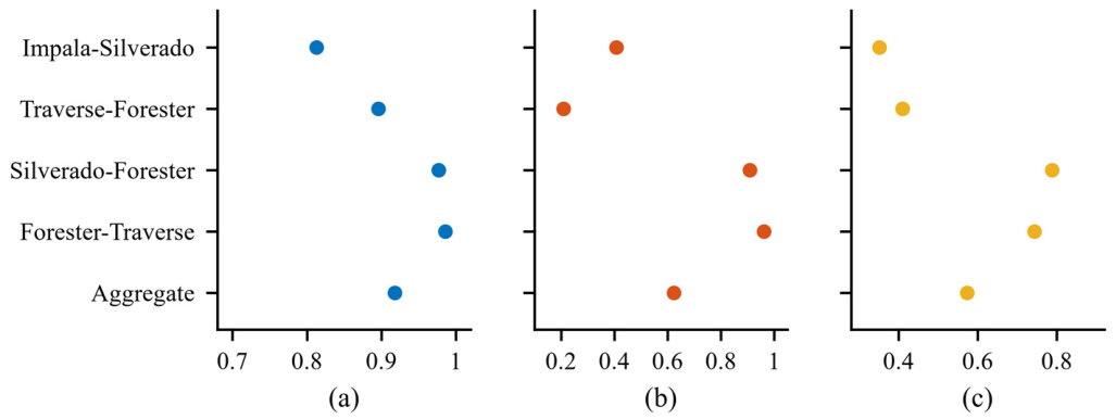
Figure 9 compares the scenario-level AUROC, AUPRC, and MCC point estimates. Silverado/Forester and Forester/Traverse had the highest AUPRC and MCC, while Traverse/Forester combined had an AUROC of 0.896 with an AUPRC of 0.210. The aggregate values summarize these distinct performance regimes.

Figure 9. Scenario-level performance of residual IF: (a) AUROC; (b) AUPRC; (c) MCC. Points show the individual scenario estimates and their four-scenario aggregate. Between-scenario sample SDs are reported in Table 2.

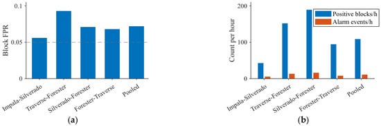
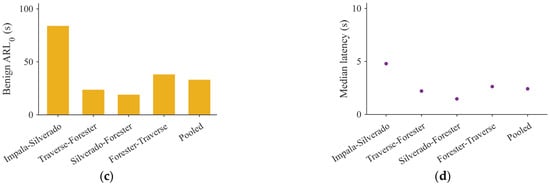
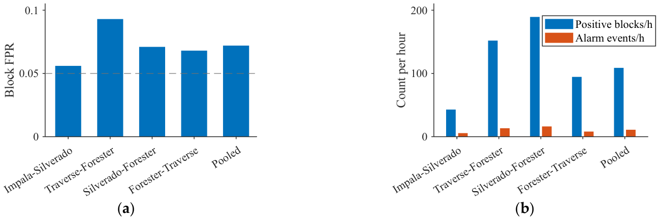
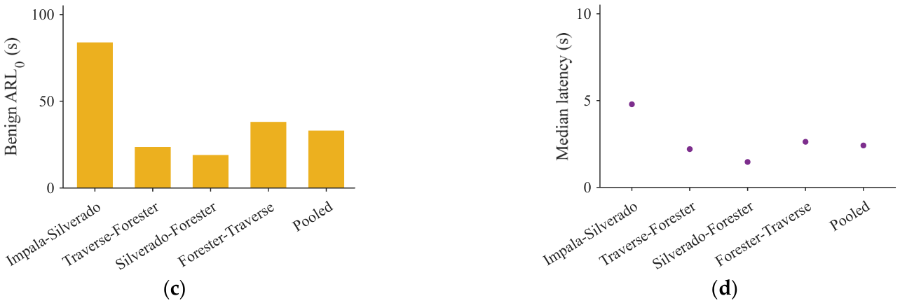
At α = 0.05, merged false-alarm rates ranged from 5.6 to 16.1 events per hour, and benign-state average run length ranged from 19.0 to 83.9 s (as shown in Figure 10).

Figure 10. EBR operational alarm metrics at α = 0.05: (a) benign-block FPR; (b) positive benign blocks and false-alarm events per hour; (c) benign-state average run length; (d) median latency among detected captures. Scenario estimates and the pooled summary are shown separately. Events use a 10 s merge horizon and 30 s refractory interval. The dashed line indicates the nominal block FPR at α = 0.05.

Block FPR ranged from 0.056 to 0.093, with Traverse/Forester farthest above the nominal α = 0.05. Silverado/Forester produced 189.3 positive blocks and 16.1 merged events per hour; Impala/Silverado produced 42.9 blocks and 5.6 events per hour. Benign-state average run length varied inversely with false alarms, and median detection delay increased with scenario-specific block duration (Figure 10).

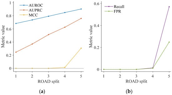
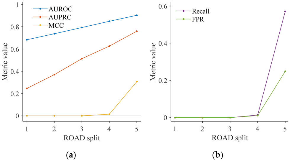
ROAD recall and FPR varied sharply with the commissioning split. Splits 1–3 produced neither positive attack blocks nor positive benign blocks. Split 4 reached a recall of 0.014 and FPR of 0.011; split 5 reached a recall of 0.571 and FPR of 0.249 (Figure 11). Table A2 reports the underlying confusion matrices.

Figure 11. Split-level stability of the ROAD target-refitted residual IF: (a) AUROC, AUPRC, and MCC; (b) attack-block recall and block FPR across five file-level splits.

ROAD AUROC and AUPRC ranged from 0.683 and 0.246 in split 1 to 0.903 and 0.760 in split 5. Per-split MCC values were 0, 0, 0, 0.014, and 0.307, yielding a mean of 0.064 and a sample SD of 0.136 (Figure 11; Table A2).

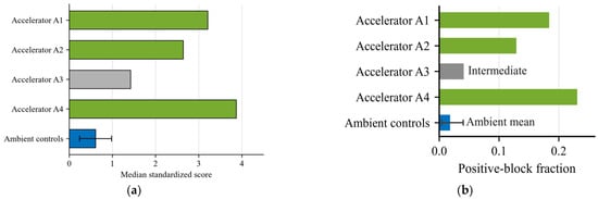
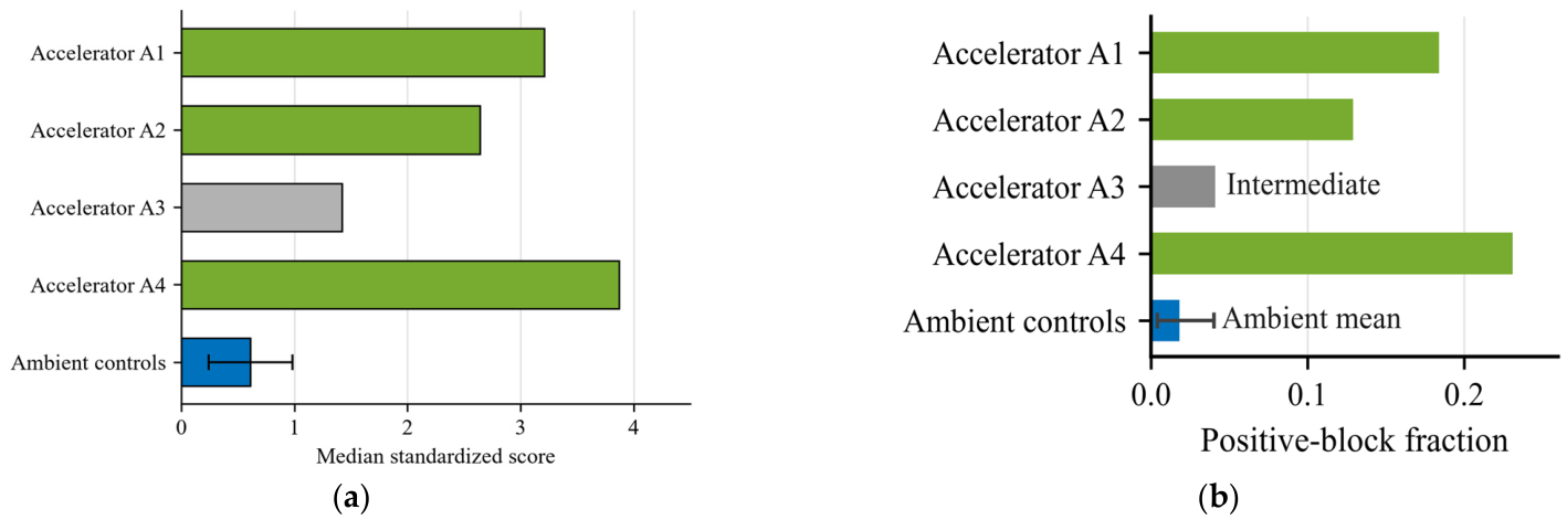
The separate accelerator analysis compared four post-exploit captures with ten ambient controls using capture-level median standardized scores and positive-block fractions (Figure 12).

Figure 12. Exploratory accelerator/post-exploit capture profile on ROAD: (a) median standardized score; (b) positive-block fraction. Green marks the three captures with the largest values, gray marks Accelerator A3, and blue summarizes ambient controls.

Accelerator A1, A2, and A4 had median standardized scores of 3.21, 2.64, and 3.87 and positive-block fractions of 0.184, 0.129, and 0.231. Accelerator A3 reached 1.42 and 0.041, compared with ambient-control means of 0.61 and 0.018 (Figure 12).

Across the five ROAD splits, residual IF achieved an AUROC of 0.793 (SD 0.087) and AUPRC of 0.503 (SD 0.203). At α = 0.05, recall was 0.117 (SD 0.254), block FPR was 0.052 (SD 0.110), and MCC was 0.064 (SD 0.136). Attack-block prevalence ranged from 0.285 to 0.482 (Table A2). Table 3 compares the ROAD configurations under the same commissioning protocol.

Table 3. ROAD workflow replication with target-specific commissioning. Values are mean (sample SD) across five overlapping file splits. MCC, attack-block recall, and block FPR use the default α = 0.05 block decisions.

Method	AUROC	AUPRC	MCC	Attack-Block Recall	Block FPR
Source-only role IF	0.519 (0.093)	0.270 (0.095)	−0.009 (0.026)	0.026 (0.059)	0.028 (0.054)
Target-adapted role IF	0.522 (0.085)	0.282 (0.068)	0.024 (0.088)	0.040 (0.088)	0.017 (0.031)
Target-refitted residual IF (primary)	0.793 (0.087)	0.503 (0.203)	0.064 (0.136)	0.117 (0.254)	0.052 (0.110)
Hybrid role + residual	0.666 (0.073)	0.381 (0.129)	0.015 (0.086)	0.051 (0.113)	0.027 (0.051)

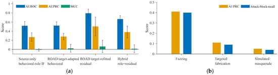
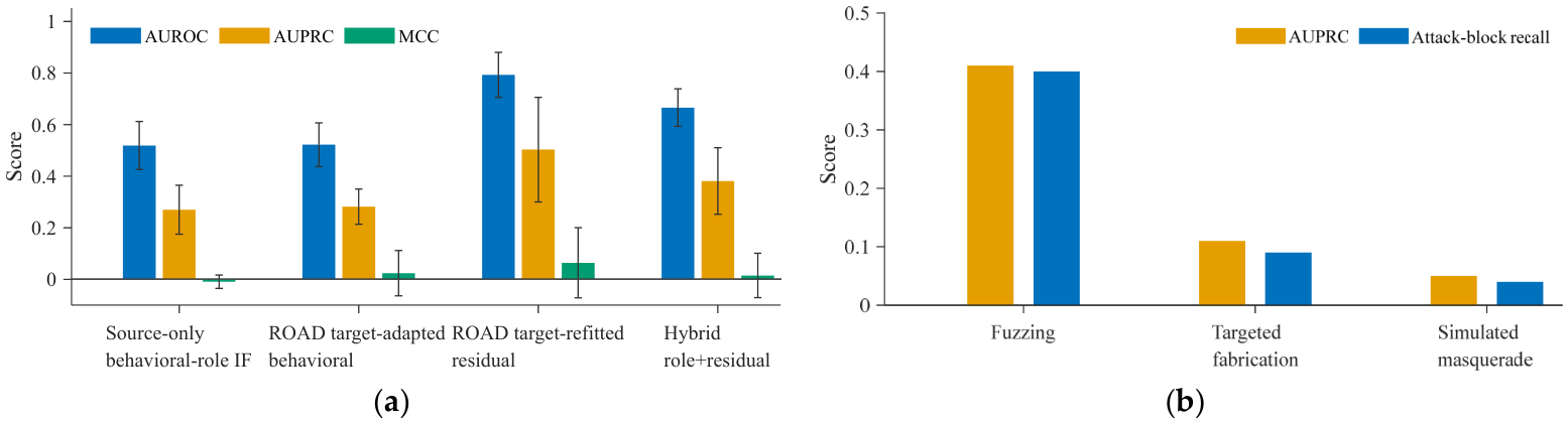
Residual IF had the highest mean AUROC and AUPRC among the ROAD configurations. Its AUPRC of 0.503 exceeded adapted-role IF at 0.282 and the hybrid configuration at 0.381 (Table 3; Figure 13a).

Figure 13. ROAD target-specific detection: (a) detector comparison, with error bars showing sample SD across five splits; (b) attack-family performance of the primary residual IF. Detector configurations are defined in Table 3.

Fuzzing produced the strongest ROAD family-level performance, with AUPRC and recall both being approximately 0.4. Targeted fabrication and simulated masquerade remained below approximately 0.12 (Figure 13b). These frame-level attack families were evaluated separately from the accelerator post-exploit profiles.

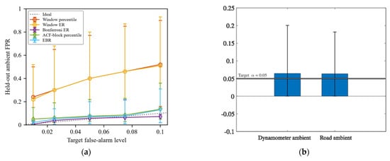
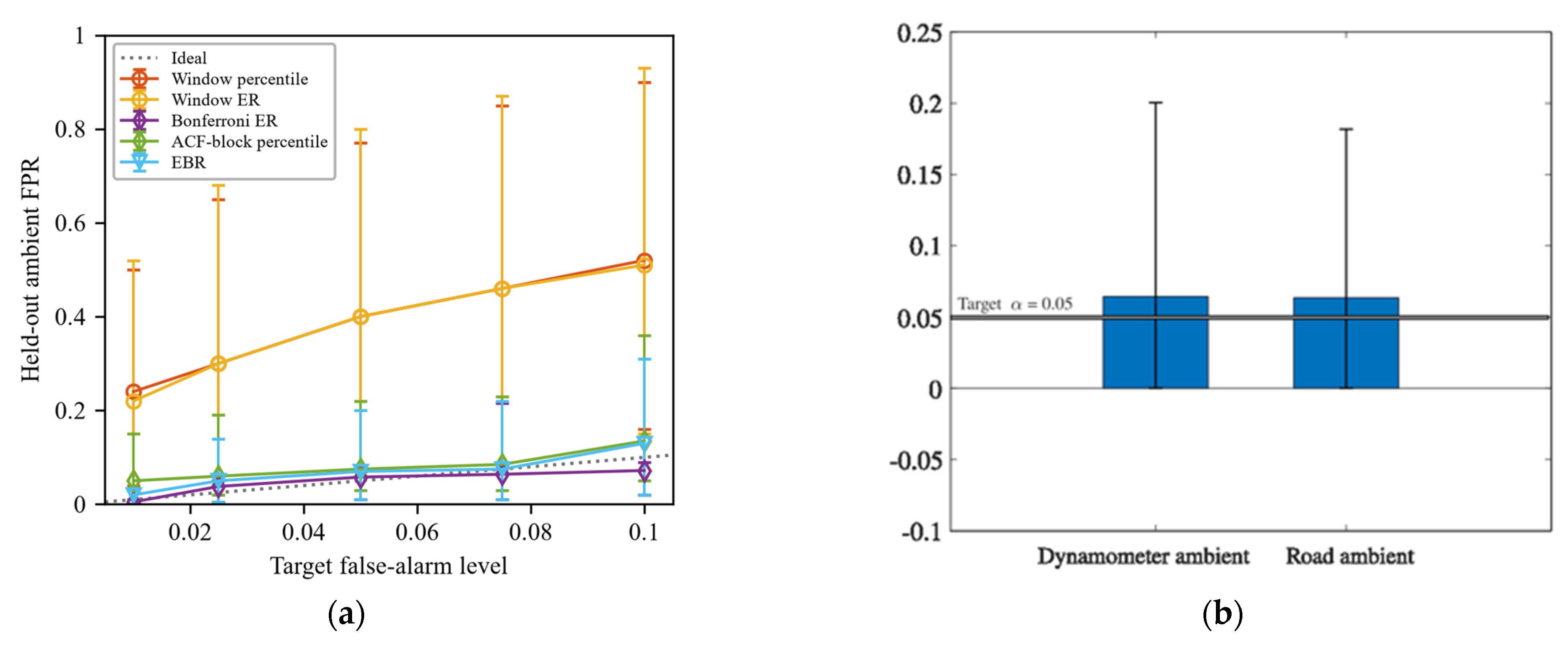
Uncorrected window rules exceeded requested FPR levels across the α range, while block-based rules tracked them more closely (Figure 14a). Held-out dynamometer and road-driving ambient traffic had similar mean FPRs near but above 0.05; across-split dispersion exceeded the mean difference between driving conditions (Figure 14b).

Figure 14. ROAD calibration: (a) empirical FPR across requested α levels for Window Percentile, Window ER, Bonferroni ER, ACF-Block Percentile, and EBR; (b) benign-condition FPR shift at α = 0.05.

3.5. Robustness and Operational Sensitivity Analyses

Table 4 summarizes the capture-separation, matched normal-only baseline, and controlled contamination analyses.

Table 4. Capture-separation, normal-only baseline, and 5% target-normal contamination results. Values are scenario-aggregated point estimates.

Configuration or Method	AUROC	AUPRC	MCC	Attack-Block Recall	Block FPR
Capture-partition sensitivity analysis
Same-capture chronological	0.918	0.622	0.573	0.786	0.072
Capture-disjoint	0.889	0.553	0.486	0.714	0.079
Leave-one-capture-out	0.875	0.521	0.451	0.681	0.083
Stronger normal-only baselines
Target-normal raw IF	0.879	0.505	0.472	0.682	0.077
MLP-AE	0.892	0.546	0.492	0.701	0.080
LSTM-AE	0.903	0.578	0.526	0.728	0.078
Deep SVDD	0.910	0.600	0.555	0.749	0.075
TCN-AE	0.914	0.609	0.562	0.762	0.074
Residual IF	0.918	0.622	0.573	0.786	0.072
Diagnostic at 5% target-normal contamination
Adaptation only	0.894	0.556	0.501	0.719	0.074
Calibration only	0.913	0.601	0.538	0.676	0.057
Adaptation and calibration	0.892	0.548	0.492	0.701	0.065

TCN-AE was the closest neural comparator to residual IF, reaching an AUPRC of 0.609 and MCC of 0.562. Deep SVDD reached 0.600 and 0.555 (Table 4). At 5% joint contamination, AUPRC was 0.548, and MCC was 0.492. Calibration-only contamination yielded an AUPRC of 0.601, recall of 0.676, and block FPR of 0.057.

Capture-disjoint and LOCO AUPRC values fell from 0.622 to 0.553 and 0.521, with absolute decreases of 0.069 and 0.101 (11.1% and 16.2%). MCC fell from 0.573 to 0.486 and 0.451, and recall decreased from 0.786 to 0.714 and 0.681, while block FPR increased from 0.072 to 0.079 and 0.083 (Table 4). Table A3 lists the capture assignments and LOCO pools.

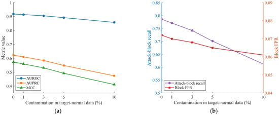
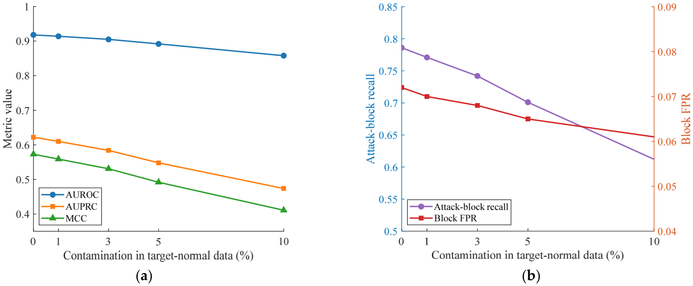
Joint commissioning contamination progressively reduced ranking and detection performance (Figure 15). At 5%, AUROC, AUPRC, MCC, and recall decreased by 0.026, 0.074, 0.081, and 0.085. Block FPR also fell from 0.072 to 0.065, together with recall and ranking quality. Performance declined further at 10%.

Figure 15. Sensitivity to target-normal contamination from 0% to 10%: (a) AUROC, AUPRC, and MCC; (b) attack-block recall and block FPR.

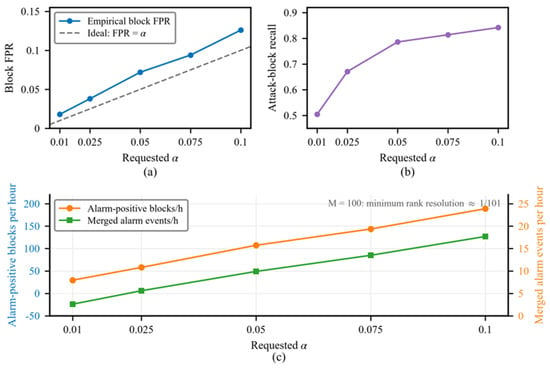
Increasing α from 0.01 to 0.10 increased FPR, recall, and alarm burden (Figure 16). At α = 0.05 in this sweep, FPR was 0.072, and recall was 0.786; approximately 108 positive blocks per hour resulted in approximately 10 merged alarm events per hour with the default 10/30 s event settings.

Figure 16. EBR operating-level tradeoff: (a) block FPR; (b) attack-block recall; (c) alarm-positive blocks and merged alarm events per hour. The α grid begins at 0.01 because M = 100 provides a rank resolution of approximately 0.0099.

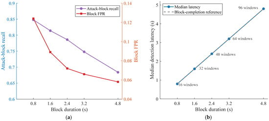
Increasing block duration from 0.8 to 4.8 s reduced FPR from approximately 0.124 to 0.059 and recall from 0.848 to 0.684, while median latency increased from 0.8 to 4.8 s (Figure 17). The 48-window (2.4 s) condition represents the median selected scale across the 20 primary scenario-seed runs; primary block lengths remained scenario-specific.

Figure 17. Block-length sensitivity across 16, 32, 48, 64, and 96 windows: (a) block FPR and attack-block recall; (b) median latency among detected captures.

4. Discussion

The matched comparisons support the contribution of target-local residual features to CAN attack detection. Under IF, residual inputs improved AUPRC by 0.117 over raw target-normal features, whereas the IF–OCSVM difference on residual inputs was 0.035. TCN-AE and Deep SVDD also approached the primary IF result on the common residual representation. Payload ablation produced the largest decrease, with timing, transitions, and identifier-use terms contributing additional evidence. Vehicle-relative ranks reduced identifier-signature MMD but retained vehicle information in full-window classifiers, explaining their role as configuration diagnostics alongside the target-local detector.

The scenario variation shows the importance of commissioning coverage and test composition. Silverado/Forester and Traverse/Forester share a target model name yet differ substantially in AUPRC. Recording conditions, attack families, prevalence, and normal-state coverage vary together in these dataset pairings. Capture-disjoint and LOCO evaluations reduced AUPRC by 11.1% and 16.2%, respectively, while lowering recall and increasing FPR. These results indicate a sensitivity to conditions beyond the chronological holdout. ROAD extends the same fitting and calibration procedure to another dataset, where split 5 contributed most detections and false alarms. It establishes workflow replication with target-specific refitting and exposes sensitivity to the selected normal files.

Calibrating block maxima accounted for most of the false-alarm reductions relative to any-window aggregation. ACF-Block Percentile and EBR share the block length and calibration maxima; EBR adds the smoothed upper-tail rank, tie handling, and attainable finite-sample tail levels. Their recall difference at matched FPR was 0.009. The main operational change therefore came from the decision unit, with the empirical rank rule providing a smaller refinement. The 2.4 s scale represents the median selected block length under the rank-resolution constraint. Longer blocks reduced FPR but also lowered recall and delayed alarms; longer trusted commissioning streams would provide more calibration maxima at the selected scale.

The fixed references and calibration make long-term normal-state coverage a further concern. Driving patterns, component aging, or seasonal temperatures can shift benign residual scores into the calibrated upper tail and increase false alarms. Periodic re-commissioning on independently trusted normal data or sequential adaptive calibration [34,35,36] offers an extension to the fixed evaluation procedure. Updates would need a trusted-data gate to distinguish benign change from attack traffic. The random attack-window substitution experiment measures dispersed contamination; contiguous sessions, identifier-specific poisoning, and contamination coordinated with operating conditions require evaluation of their temporal and feature-level effects. Novel benign states should be assessed separately from malicious poisoning, with longitudinal studies tracking both false alarms and attack recall.

The weaker targeted-fabrication and simulated-masquerade results are consistent with the statistical content of the residual vector. Byte deviations, timing, identifier use, and transitions respond to communication changes, but low-rate manipulations can preserve these distributions while altering signal meaning. Window summaries can further dilute sparse changes. A semantics-aware layer could add decoded-signal plausibility, rates of change, and cross-signal or vehicle-state consistency [12,13]. This extension would require vehicle-specific definitions, such as DBC files, and trusted normal signal coverage. Evaluation should include subtle attacks, benign state changes, and manipulations that retain physically plausible trajectories.

The pooled 11.1 false-alarm events per hour correspond to an interruption about every 5–6 min. Direct driver warnings at this rate would be disruptive, while fleet monitoring would increase Security Operations Center (SOC) workload. Lower α, event triage, and complementary detection evidence offer routes to alarm reduction, with associated recall and latency trade-offs. The reported 9222 frames/s is batch software throughput. Deployment assessment needs ECU memory use, scheduling behavior, and online latency measured through window accumulation, block completion, scoring, and event processing.

The evaluation covers four can-train-and-test pairings with three named target models—Silverado, Forester, and Traverse—and one ROAD vehicle. Reused captures and overlapping ROAD splits constrain the estimates to the evaluated datasets. Independent vehicles, sites, and driving sessions would broaden normal-state coverage and test the observed sensitivity. The accelerator analysis profiles four post-exploit captures; capture-level classification would need a threshold assessed on independent captures.

Further work should combine independent-drive validation with structured poisoning and drift experiments and prospective event-level assessment. Ensembles of residual and semantic learners, supported by feature attribution, offer a direction for combining complementary evidence and explaining alarm causes [24,25,26]. Their added detection value should be measured under the same trusted commissioning and event-level protocol.

5. Conclusions

This study developed a 12-dimensional target-normal residual representation and a dependence-informed block-calibration workflow for CAN intrusion detection. Each vehicle supplies trusted normal commissioning data for local reference estimation, detector fitting, and calibration. Across four can-train-and-test scenarios, residual IF achieved a mean AUPRC of 0.622 and MCC of 0.573. Matched comparisons and ablations identified contributions from payload, timing, transitions, and identifier use. Block-maximum calibration provided the main false-alarm reduction, while EBR supplied a smaller refinement to the rank-based decision rule.

Capture-separated evaluations and ROAD replication showed sensitivity to normal-data coverage and recording conditions. ROAD AUPRC reached 0.503 after target-specific refitting, with strong split-level variation and better detection of fuzzing than subtle semantic attacks. The remaining 11.1 false-alarm events per hour define a practical priority for further development. Independent-drive validation, trusted drift adaptation, semantic evidence, and online hardware measurements should extend the present workflow.

References

- Tanksale, V. Intrusion detection system for controller area network. Cybersecurity 2024, 7, 4. [Google Scholar] [CrossRef] [Scilit]
- Fayyaz Khan, O.; Mubashir, M.; Iqbal, J. Comprehensive review of CAN bus security: Vulnerabilities, cryptographic and IDS approaches, and countermeasures. J. Eng. Technol. Appl. Phys. 2025, 7, 19–26. [Google Scholar] [CrossRef] [Scilit]
- Rai, R.; Grover, J.; Sharma, P.; Pareek, A. Securing the CAN bus using deep learning for intrusion detection in vehicles. Sci. Rep. 2025, 15, 13820. [Google Scholar] [CrossRef] [Scilit]
- Yang, H.; Effatparvar, M. A deep learning based intrusion detection system for CAN vehicle based on combination of triple attention mechanism and GGO algorithm. Sci. Rep. 2025, 15, 19462. [Google Scholar] [CrossRef] [Scilit]
- Olufowobi, H.; Young, C.; Zambreno, J.; Bloom, G. SAIDuCANT: Specification-based automotive intrusion detection using Controller Area Network (CAN) timing. IEEE Trans. Veh. Technol. 2020, 69, 1484–1494. [Google Scholar] [CrossRef]
- Bozdal, M.; Samie, M.; Jennions, I.K. WINDS: A wavelet-based intrusion detection system for Controller Area Network (CAN). IEEE Access 2021, 9, 58621–58633. [Google Scholar] [CrossRef] [Scilit]
- Lee, S.; Jo, H.J.; Cho, A.; Lee, D.H.; Choi, W. TTIDS: Transmission-resuming time-based intrusion detection system for Controller Area Network (CAN). IEEE Access 2022, 10, 52139–52153. [Google Scholar] [CrossRef] [Scilit]
- Kim, W.; Lee, J.; Lee, Y.; Kim, Y.; Chung, J.; Woo, S. Vehicular multilevel data arrangement-based intrusion detection system for in-vehicle CAN. Secur. Commun. Netw. 2022, 2022, 4322148. [Google Scholar] [CrossRef] [Scilit]
- Desta, A.K.; Ohira, S.; Arai, I.; Fujikawa, K. Rec-CNN: In-vehicle networks intrusion detection using convolutional neural networks trained on recurrence plots. Veh. Commun. 2022, 35, 100470. [Google Scholar] [CrossRef] [Scilit]
- Lo, W.; AlQahtani, H.; Thakur, K.; Almadhor, A.S.; Chander, S.; Kumar, G. A hybrid deep learning based intrusion detection system using spatial-temporal representation of in-vehicle network traffic. Veh. Commun. 2022, 35, 100471. [Google Scholar] [CrossRef] [Scilit]
- Zhang, G.; Liu, Q.; Cao, C.; Li, J.; Li, Y. Bit scanner: Anomaly detection for in-vehicle CAN bus using binary sequence whitelisting. Comput. Secur. 2023, 134, 103436. [Google Scholar] [CrossRef] [Scilit]
- Nichelini, A.; Pozzoli, C.A.; Longari, S.; Carminati, M.; Zanero, S. CANova: A hybrid intrusion detection framework based on automatic signal classification for CAN. Comput. Secur. 2023, 128, 103166. [Google Scholar] [CrossRef] [Scilit]
- Jeong, S.; Lee, S.; Lee, H.; Kim, H.K. X-CANIDS: Signal-aware explainable intrusion detection system for Controller Area Network-based in-vehicle network. IEEE Trans. Veh. Technol. 2024, 73, 3230–3246. [Google Scholar] [CrossRef] [Scilit]
- Shahriar, M.H.; Xiao, Y.; Moriano, P.; Lou, W.; Hou, Y.T. CANShield: Deep-learning-based intrusion detection framework for Controller Area Networks at the signal level. IEEE Internet Things J. 2023, 10, 22111–22127. [Google Scholar] [CrossRef] [Scilit]
- Kang, H.; Vo, T.; Kim, H.K.; Hong, J.B. CANival: A multimodal approach to intrusion detection on the vehicle CAN bus. Veh. Commun. 2024, 50, 100845. [Google Scholar] [CrossRef] [Scilit]
- Khan, M.H.; Javed, A.R.; Iqbal, Z.; Asim, M.; Awad, A.I. DivaCAN: Detecting in-vehicle intrusion attacks on a controller area network using ensemble learning. Comput. Secur. 2024, 139, 103712. [Google Scholar] [CrossRef] [Scilit]
- Sun, H.; Wang, J.; Weng, J.; Tan, W. KG-ID: Knowledge graph-based intrusion detection on in-vehicle network. IEEE Trans. Intell. Transp. Syst. 2025, 26, 4988–5000. [Google Scholar] [CrossRef] [Scilit]
- Al-Absi, G.A.; Fang, Y.; Qaseem, A.A. STC-GraphFormer: Graph spatial-temporal correlation transformer for in-vehicle network intrusion detection system. Veh. Commun. 2025, 51, 100865. [Google Scholar] [CrossRef] [Scilit]
- Xia, Z.; Huang, L.; Tan, J.; Yu, Y.; Hao, W.; Long, K. A lightweight intrusion detection system for connected autonomous vehicles based on ECANet and image encoding. J. Inf. Secur. Appl. 2025, 92, 104082. [Google Scholar] [CrossRef] [Scilit]
- Sreelekshmi, M.S.; Aji, S. A deep architecture for in-vehicle intrusion detection using controller area network-graph relied feature images. Comput. Electr. Eng. 2025, 127, 110584. [Google Scholar] [CrossRef] [Scilit]
- Cheng, P.; Liu, S.; Wu, Z.; Tan, L.; Liu, G. MKF-ADS: Multi-knowledge fusion based anomaly detection system in vehicular control area networks. IEEE Trans. Veh. Technol. 2025, 74, 13795–13808. [Google Scholar] [CrossRef] [Scilit]
- Ileri, K.; Rakib, A.; Djahel, S. MetaCAN: An optimized adaptive hybrid metaheuristic-based intrusion detection system for CAN bus security. Veh. Commun. 2025, 55, 100956. [Google Scholar] [CrossRef] [Scilit]
- Zhang, M.; Li, J.; Lai, Y.; Huan, S.; Shang, W. A lightweight voltage-based ECU fingerprint intrusion detection system for in-vehicle CAN bus. IEEE Trans. Veh. Technol. 2025, 74, 15536–15548. [Google Scholar] [CrossRef] [Scilit]
- Wang, J.; Huang, X.; Dong, L.; Ji, S.; Luo, C. Rockburst risk assessment in deep mining using ensemble models with interpretable features. Tunn. Undergr. Space Technol. 2026, 178, 108033. [Google Scholar] [CrossRef] [Scilit]
- Cai, X.; Wang, Y.; Zhao, Y.; Chen, L.; Wang, P.; Wang, Z.; Li, J. Dynamic strength prediction of brittle engineering materials via stacked multi-model ensemble learning and interpretability-driven feature analysis. Materials 2025, 18, 3054. [Google Scholar] [CrossRef] [Scilit]
- Wang, M.; Ying, F.; Yang, J.; Zhu, D. An explainable (interpretable) stacking ensemble machine learning model for real-time and short-term significant sea wave height prediction. Sustain. Energy Technol. Assess. 2026, 85, 104794. [Google Scholar] [CrossRef] [Scilit]
- Lampe, B.; Meng, W. can-train-and-test: A curated CAN dataset for automotive intrusion detection. Comput. Secur. 2024, 140, 103777. [Google Scholar] [CrossRef] [Scilit]
- Verma, M.E.; Bridges, R.A.; Iannacone, M.D.; Hollifield, S.C.; Moriano, P.; Hespeler, S.C.; Kay, B.; Combs, F.L. A comprehensive guide to CAN IDS data and introduction of the ROAD dataset. PLoS ONE 2024, 19, e0296879. [Google Scholar] [CrossRef] [Scilit]
- Kidmose, B.; Kidmose, A.; Meng, W. can-sleuth: Sleuthing out the capabilities, limitations, and performance impacts of automotive intrusion detection datasets. Int. J. Inf. Secur. 2025, 24, 193. [Google Scholar] [CrossRef] [Scilit]
- Ghadi, A.; Mohd, T.K. Learning-based intrusion detection systems for in-vehicle CAN networks: A comprehensive survey with deployment and real-time considerations. J. Braz. Comput. Soc. 2026, 32, 1755–1785. [Google Scholar] [CrossRef] [Scilit]
- Wang, X.; Zhao, J.; Liu, P.; Yao, N.; Xu, Z. CAN bus intrusion detection based on deep learning with data augmentation for connected autonomous vehicles. IEEE Trans. Veh. Technol. 2026, 75, 2253–2266. [Google Scholar] [CrossRef] [Scilit]
- Yin, Z.; Li, Z.; Zhang, Y.; Li, J.; Liu, D.; Wei, H. Temporal-spatial feature fusion based intrusion detection system for in-vehicle networks. Comput. Secur. 2026, 161, 104781. [Google Scholar] [CrossRef] [Scilit]
- El-Fatyany, A.; Wang, X.; Lu, L.; Ren, K. EF-IDS: An efficient intrusion detection system with enriched features for CAN bus in modern vehicles. J. Syst. Archit. 2026, 171, 103646. [Google Scholar] [CrossRef] [Scilit]
- Barber, R.F.; Candès, E.J.; Ramdas, A.; Tibshirani, R.J. Conformal prediction beyond exchangeability. Ann. Stat. 2023, 51, 816–845. [Google Scholar] [CrossRef] [Scilit]
- Xu, C.; Xie, Y. Conformal prediction interval for dynamic time-series. Proc. Mach. Learn. Res. 2021, 139, 11559–11569. [Google Scholar]
- Gibbs, I.; Candès, E.J. Adaptive conformal inference under distribution shift. Adv. Neural Inf. Process. Syst. 2021, 34, 1660–1672. [Google Scholar]
- Ruff, L.; Vandermeulen, R.A.; Goernitz, N.; Deecke, L.; Siddiqui, S.A.; Binder, A.; Müller, E.; Kloft, M. Deep one-class classification. Proc. Mach. Learn. Res. 2018, 80, 4393–4402. [Google Scholar]
- Thill, M.; Konen, W.; Wang, H.; Bäck, T. Temporal convolutional autoencoder for unsupervised anomaly detection in time series. Appl. Soft Comput. 2021, 112, 107751. [Google Scholar] [CrossRef] [Scilit]
- Althunayyan, M.; Javed, A.; Rana, O. A robust multi-stage intrusion detection system for in-vehicle network security using hierarchical federated learning. Veh. Commun. 2024, 49, 100837. [Google Scholar] [CrossRef] [Scilit]
Disclaimer/Publisher’s Note: The statements, opinions and data contained in all publications are solely those of the individual author(s) and contributor(s) and not of MDPI and/or the editor(s). MDPI and/or the editor(s) disclaim responsibility for any injury to people or property resulting from any ideas, methods, instructions or products referred to in the content. |
© 2026 by the authors. Licensee MDPI, Basel, Switzerland. This article is an open access article distributed under the terms and conditions of the Creative Commons Attribution (CC BY) license.