


Abstract
Physics-informed neural networks (PINNs) have recently attracted considerable attention as a framework for solving partial differential equations. Underwater sound-field prediction fundamentally relies on solving acoustic wave equations, making PINNs a natural candidate for this application. This paper reviews recent developments in PINN-based modeling of underwater acoustic propagation, which we group into two main lines of research. The first introduces mathematically motivated simplifications of the governing equations and then employs PINNs as efficient solvers; examples include ray-based PINNs and PINN estimators of modal wavenumbers. The second focuses on improving computational performance by tailoring network architectures and hyperparameters, such as spatial domain-decomposition strategies. While PINNs demonstrate significant potential, challenges persist regarding computational efficiency and convergence in high-frequency regimes. Future research directions are identified, emphasizing a multi-faceted strategy that systematically addresses limitations at both the physical formulation level and the neural network architecture level. By integrating advanced hybrid physics-data modeling and scalable training algorithms, this review highlights the pathway toward bridging the gap between theoretical frameworks and realistic ocean applications.
1. Introduction
Driven by hardware innovations and algorithmic optimizations, recent advancements in computational infrastructure have catalyzed unprecedented progress in neural network architectures [1,2]. These models have achieved remarkable success across diverse domains, including computer vision (e.g., autonomous driving), natural language processing, generative artificial intelligence, and image synthesis. In the wake of these developments, the scientific community increasingly recognizes the transformative potential of integrating machine learning with engineering and physical sciences. This convergence has positioned “AI for Science” as a burgeoning frontier, garnering significant research attention worldwide.
The evolution of scientific discovery was succinctly characterized by Turing Award laureate Jim Gray through four distinct paradigms: experimental, theoretical, computational, and data-intensive science. The fourth paradigm focuses on distilling insights from massive datasets that remain intractable for traditional methodologies. In this context, data-driven machine learning has emerged as a fundamental instrument, excelling at the modeling and analysis of such substantial volumes of information [3].
The potential of machine learning, however, extends far beyond existing applications. “AI for Science” represents a cutting-edge convergence of machine learning and natural sciences, a synergy exemplified by breakthroughs such as AlphaFold2 [4], which demonstrated superhuman capabilities in resolving intricate biological challenges. Microsoft Research posits that machine learning holds the unique promise of reconciling the often-competing demands of computational speed and physical accuracy in scientific discovery. Propelled by this vision, initiatives such as the AI4Science research center have been established, dedicated to leveraging artificial intelligence to develop novel tools for exploration and to pioneer a fifth paradigm of scientific discovery.
Within this broader landscape, “AI for PDE” has emerged as a pivotal branch, focusing on the deployment of deep learning methodologies to approximate solutions to partial differential equation (PDE). These mathematical problems are conventionally categorized into two types: forward problems, which involve solving for field variables given known boundary conditions, initial conditions, and equation parameters; and inverse problems, which aim to infer unknown coefficients or boundary conditions by assimilating observational or experimental data into the PDE framework.
In scientific and engineering domains, PDEs serve as the fundamental language for describing complex physical phenomena. While traditional numerical methods remain effective for standard applications, they often face prohibitive computational bottlenecks when applied to high-dimensional or highly nonlinear systems. Recent advances in deep learning offer a transformative alternative to these limitations. By approximating solutions in a mesh-free paradigm leveraged by automatic differentiation [5], neural networks effectively mitigate the curse of dimensionality. Moreover, they provide a flexible framework that enables the direct inversion of PDE parameters from sparse data—a capability that distinctively sets them apart from conventional numerical approaches.
AI methodologies for solving PDEs can be categorized into two primary frameworks based on their core principles:
- Neural surrogate networks: exemplified by architectures such as Fourier Neural Operator (FNO) [6] and DeepONet [7], which learn mappings between input functions and PDE solutions. However, such data-intensive approaches have seen limited application and research in underwater acoustics, primarily due to their substantial data requirements which are often incompatible with the sparse data reality of ocean environments. Consequently, these methods fall beyond the scope of the present study.
- Neural PDE solvers: typified by Physics-Informed Neural Networks (PINNs), which directly embed physical laws (e.g., governing equations, boundary conditions) into the training loss.
Traditional data-driven methods for approximating PDE solutions suffer from critical limitations, most notably their heavy reliance on large-scale, high-quality datasets. Furthermore, these approaches often exhibit poor extrapolation capabilities beyond the training domain, limited robustness, and a lack of interpretability [8]. A significant concern is that, without explicit constraints, purely data-driven models may yield solutions that fundamentally violate governing physical principles.
In contrast to task-specific solvers, neural operators are designed to approximate nonlinear mappings between infinite-dimensional function spaces. This capability enables them to solve entire families of PDEs across diverse initial conditions, boundary conditions, and geometries, making them particularly advantageous for high-dimensional and multi-input/multi-output problems. However, training neural operators typically demands extensive paired input-output datasets, which necessitate computationally expensive numerical simulations or are limited by sparse experimental observations. Moreover, their inability to explicitly incorporate governing equations can lead to generalization failures under distribution shifts and result in physically inconsistent predictions. These challenges underscore the urgent need for hybrid methodologies that seamlessly integrate data-driven learning with physics-based constraints.
PINN was originally proposed by Raissi, Perdikaris, and Karniadakis [9], constitute the core methodology of this study. Designed for supervised learning, PINNs explicitly encode physical constraints within their loss functions, including governing equations and boundary conditions. This formulation systematically penalizes outputs that violate physical principles, thereby significantly constraining the search space for nonlinear optimization and alleviating the dependence on massive datasets. Consequently, observational data transitions from being the primary driver to playing an auxiliary role in the learning process. PINNs demonstrate distinct advantages in solving both forward and inverse problems for nonlinear PDE systems, delivering robust, interpretable, and physically consistent solutions even in regimes characterized by sparse or noisy data.
Since their inception, PINNs have garnered substantial attention from the scientific community. Research leveraging PINNs has expanded rapidly, with applications spanning fluid dynamics, solid mechanics, heat transfer, and electromagnetic modeling, thereby establishing PINNs as a dominant for PDE solving via deep learning [10]. This methodology has matured through extensive theoretical refinements and robust practical implementations. Notably, the development of specialized software ecosystems has streamlined PINN deployment: Lu et al. introduced DeepXDE [11], an open-source Python framework tailored for physics-informed deep learning, while NVIDIA released Modulus, a GPU-accelerated platform designed for simulating complex nonlinear physical systems. These standardized toolkits, alongside a vibrant community of open-source repositories, have significantly democratized access to PINN research and applications.
The proliferation of these frameworks has catalyzed significant methodological advancements, including the development of adaptive sampling strategies, hybrid architectures such as domain decomposition (e.g., XPINNs [12]), and rigorous uncertainty quantification techniques [13]. As PINNs transition from theoretical constructs to industrial-grade tools, their adoption is expanding across domains that demand real-time simulation, multi-physics coupling, and inverse design optimization. This trajectory underscores the unique capacity of PINNs to bridge the gap between data-driven machine learning and traditional computational physics paradigms.
In the context of the ocean environment, acoustic waves represent the sole effective medium for long-range wireless information transmission. Consequently, understanding sound propagation through the ocean constitutes the physical foundation for analyzing and predicting hydroacoustic phenomena. This knowledge enables critical applications such as underwater detection, localization, identification, and tracking—capabilities that hold strategic significance for underwater sensing networks, submersible platforms, and naval operations.
Underwater acoustic field modeling, a cornerstone of ocean acoustics, fundamentally entails solving the acoustic wave equation [14]. However, obtaining closed-form analytical solutions to this equation in realistic ocean settings is generally intractable. Historically, researchers have relied on asymptotic approximations and simplifying assumptions to derive numerical solutions using established models, including ray theory [15], Normal Mode methods [16], Parabolic Equation (PE) methods [17], and the Finite Element Method (FEM) [18]. While these traditional methods have substantially advanced the field, they exhibit inherent limitations, such as restricted domains of applicability and a strong sensitivity to spatially and temporally variable environmental parameters (e.g., sound speed profiles and seabed properties).
The spatiotemporally dynamic nature of the ocean presents a fundamental challenge in underwater acoustics. Applications pertaining to ocean acoustic propagation modeling are primarily categorized into two domains: forward problems and inverse problems, as illustrated in Figure 1. Forward problems involve predicting the acoustic field distribution at receiver locations given known environmental parameters and source configurations. Conversely, inverse problems focus on inferring unknown environmental characteristics (e.g., sound speed profiles or geoacoustic parameters) from measured acoustic data.
Figure 1.
Schematic illustration of (a) the forward problem and (b) the inverse problem in ocean acoustics. (a) The forward problem involves predicting the acoustic field distribution within an Area of Interest (AOI) or at specific receiver locations, given known environmental parameters (e.g., SSP, BTY) and source configurations. (b) The inverse problem focuses on inferring unknown environmental characteristics or source parameters from sparse acoustic data measured by arrays (e.g., VLA). SSP: Sound Speed Profile; BTY: Bathymetry; AOI: Area of Interest; VLA: Vertical Line Array.
The emergence of PINNs holds transformative potential for addressing these challenges. Unlike conventional numerical methods, which often rely on computationally intensive grid generation and approximate data assimilation schemes, PINNs facilitate the seamless integration of governing physical laws with sparse observational data. Beyond their demonstrated capability in solving forward problems, PINNs offer a unique advantage in inverse modeling. By embedding the acoustic wave equation directly into the loss function, they can simultaneously reconstruct the wavefield and identify key environmental parameters, such as spatially varying sound speed profiles and seabed reflection coefficients, thereby presenting a robust and flexible alternative to traditional inversion approaches.
While several reviews have summarized the progress of PINNs in general mechanics [8,19] or data-driven machine learning in ocean acoustics [20,21], a dedicated survey focusing specifically on PINN-based underwater acoustic modeling remains absent. Existing reviews typically overlook the unique challenges associated with solving the high-frequency Helmholtz equation and handling large-scale, heterogeneous ocean environments. This paper fills this critical gap by providing a comprehensive review of PINNs applied to underwater acoustic propagation, systematically analyzing their inherent challenges, and outlining promising directions for future development.
In the field of underwater acoustics, the prevalence of narrowband signal applications renders the frequency-domain Helmholtz equation the predominant governing model, often taking precedence over time-domain wave equation formulations. Consequently, direct time-domain solutions have received comparatively limited attention in the context of efficient propagation modeling [22]. Furthermore, while the heterogeneous ocean medium dictates the acoustic refractive index, boundary conditions at the sea surface and seabed are routinely approximated according to the scale of the problem. Accordingly, this review explicitly excludes time-domain modeling, strongly nonlinear acoustic phenomena, and complex fluid–structure or flow–acoustic interactions. Instead, our discussion is centered on acoustic fields governed by the Helmholtz equation within realistic oceanic environments—a regime that encompasses the vast majority of practical applications in sonar, underwater communications, and environmental acoustics.
The remainder of this paper is organized as follows: Section 2 outlines the general theoretical framework of PINNs and elaborates on the ocean acoustic prediction problem. Section 3 comprehensively reviews recent advances in PINN-based methodologies for underwater acoustic propagation. Building upon the intrinsic characteristics of PINNs and the current state of the art, Section 4 provides a critical synthesis of the technical challenges encountered in PINN-based acoustic field prediction. Following this, Section 5 envisions future research directions, proposing systematic solutions to advance PINN applications in the underwater acoustics domain. Finally, Section 6 concludes the paper with a summary of the key findings.
2. Physical-Informed Neural Network (PINN) and Ocean Acoustics
The concept of PINNs was originally proposed by Raissi, Perdikaris, and Karniadakis [9]. Since then, PINNs have attracted considerable attention as a physics-informed learning framework for solving forward and inverse problems governed by partial differential equations (PDEs). A key idea of PINNs is to embed governing equations, conservation laws, and prior knowledge directly into the training objective, thereby reducing reliance on large, supervised datasets.
Unlike conventional numerical solvers, which typically require mesh generation and discretization of the computational domain in space and/or time, PINNs represent the solution using a neural network and exploit automatic differentiation (AD) to evaluate differential operators appearing in the PDE. This mesh-free formulation can simplify handling complex geometries and enables a unified treatment of forward simulation and parameter identification within a single optimization framework.
A standard PINN implementation uses a multi-layer perceptron (MLP) with fully connected layers to approximate the target field variables (e.g., pressure or particle velocity) as a function of spatial coordinates and, when needed, time. Physical consistency is enforced by penalizing the PDE residual, obtained by substituting the network output into the governing differential operators. A typical loss function is formulated as
where measures the mismatch between the network prediction and available observations, and enforces adherence to the governing PDE through the residual loss. The weighting parameter controls the balance between data fidelity and physical consistency.
By minimizing composite loss using gradient-based optimization, PINNs aim to satisfy the underlying physics while fitting observations in the training domain. As a result, they can provide physically consistent predictions at unobserved locations and support inverse inference of unknown parameters when data are sparse or noisy.
For the ocean acoustic problems considered in this study, sound propagation is governed by the acoustic wave equation. Under the simplifying assumptions of an acoustically homogeneous fluid with constant density and constant sound speed c, the homogeneous wave equation for the acoustic pressure reads:
where represents the sound pressure, c denotes the sound speed in seawater, and t represents time.
Given the prevalence of narrowband signals in underwater acoustics, it is common practice to transform the time-domain wave equation into the frequency domain. By applying the Fourier transform, we obtain the Helmholtz equation, which governs monochromatic wave propagation. In a cylindrical coordinate system, this equation is written as:
where denotes the horizontal range, is the depth, and is the wavenumber corresponding to the angular frequency . This frequency-domain formulation effectively transforms the original hyperbolic time-dependent problem into an elliptic boundary value problem (steady-state). This transformation facilitates computationally efficient modeling of harmonic wave propagation, particularly in contexts dominated by frequency-specific phenomena.
The structural diagram of a standard PINN applied to ocean acoustics is presented in Figure 2. A critical consideration in this domain is that the acoustic pressure field is inherently complex-valued, whereas conventional neural network frameworks typically operate on real-valued domains. To circumvent this constraint, prevalent methodologies implement a component-wise strategy: the complex pressure field is decoupled into its real and imaginary components. These components are subsequently treated as distinct output channels within the network architecture, with the governing Helmholtz equation split into a coupled system of two real-valued PDEs [23].
Figure 2.
The structure diagram of standard PINN for ocean acoustics.
Obtaining a unique solution to the wave equation necessitates the imposition of appropriate boundary conditions, which include source excitation terms and physical domain boundaries. In ocean acoustics, sources are conventionally modeled as idealized point sources represented by the Dirac delta function. However, since the Dirac delta is singular and non-differentiable, posing severe challenges for automatic differentiation. A common computational practice is to approximate it using a Gaussian function with a finite width. This substitution provides a smooth, differentiable representation that ensures numerical stability during the training of the neural network.
Regarding domain boundaries, the sea surface is typically characterized as a pressure-release boundary. This imposes a Dirichlet boundary condition where the acoustic pressure vanishes (i.e., ). Conversely, the seabed boundary involves complex interactions, including reflection, scattering, and transmission into sediment layers.
Modeling the seabed is mathematically nontrivial, as it may require frequency-dependent impedance boundary conditions or continuity conditions across fluid–elastic interfaces. To reduce model complexity and improve training stability, many existing PINN-based studies adopt simplified bottom representations. A preliminary choice is a rigid (sound-hard) boundary, i.e., a Neumann condition enforcing zero normal particle velocity, which corresponds to an idealized perfectly reflecting seabed. Alternatively, some works avoid explicit seabed modeling by prescribing boundary information through auxiliary sound pressure data along the bottom boundary. While these simplifications reduce computational burden, they may introduce non-negligible modeling errors in scenarios where seabed properties strongly influence acoustic propagation.
3. Current Applications and Developments of PINNs
Since their introduction, PINNs have garnered significant research interest for solving acoustic problems. Their theoretical foundation stems from the Universal Approximation Theorem [24,25], which asserts that feedforward neural networks with sufficient hidden neurons can approximate any continuous function to arbitrary precision. This theorem provides the essential mathematical justification for the capacity of neural networks to represent the complex solution manifolds of PDEs.
Nevertheless, persistent challenges hinder the practical implementation of PINNs in acoustics. The intrinsic stiffness of acoustic wave equations, coupled with the spectral bias inherent in MLPs [26], frequently results in inadequate convergence at critical regions of the solution. Specifically, even as the global loss decreases during optimization, localized features such as discontinuities, sharp gradients, and high-frequency wave components often fail to resolve accurately. This limitation arises because the standard residual minimization objective (e.g., Mean Squared Error) inherently prioritizes low-frequency, smooth components of the solution, thereby struggling to capture the high-frequency oscillations or steep gradients that are characteristic of acoustic wavefields.
The ocean acoustic environment is inherently defined by multiscale dynamics, ranging from millimeter-scale turbulence to basin-scale variations spanning hundreds of kilometers. Concurrently, many active sonar and communication systems rely on high-frequency acoustic waves to achieve fine spatial resolution. This combination of large-scale domains and short-wavelength oscillations presents formidable computational challenges for standard PINNs [27].
Through a systematic review of the extant literature, we categorize prevailing methodologies into two principal classes, as illustrated in Figure 3:
Figure 3.
Taxonomy of PINN-based methodologies for ocean acoustics, categorized into modifications based on conventional models and performance-enhancement strategies.
- Modifications based on conventional models: These approaches integrate PINNs with established numerical frameworks (i.e., ray theory, normal modes, or PE models) to incorporate physical priors, thereby enhancing compatibility with specific propagation regimes or reducing computational complexity.
- Modifications based on network architecture: These innovations focus on improving the solver itself and span several critical areas, including neural architecture modifications, hyperparameter optimization, and training strategy advancements. The latter encompasses techniques such as adaptive loss weighting schemes, domain decomposition, and sophisticated optimization algorithms designed to navigate the complex loss landscape of acoustic problems.
These two classes of methodologies manifest divergent efficacy in addressing domain-specific challenges, revealing distinct intrinsic strengths and limitations. Hybrid models that incorporate conventional solvers frequently excel in computational efficiency and convergence speed; however, their accuracy is inherently bounded by the asymptotic approximations endemic to the underlying physical models. Conversely, architecture-driven enhancements demonstrate superior capabilities without physical simplifications. Yet, demand considerable computational resources for training and require meticulous hyperparameter tuning.
3.1. Direct Application of PINNs for Solving Acoustic Governing Equations
This section reviews studies that directly apply PINNs to solve the fundamental governing equations of acoustics. Based on the domain of the problem, existing works can be broadly classified into time-domain wave equation solvers and frequency-domain Helmholtz equation solvers. While these direct solvers aim to capture full-wave physics without asymptotic approximations, they face distinct challenges when applied to realistic underwater environments.
3.1.1. Time-Domain Wave Equation Modeling
Direct time-domain PINNs have primarily been explored as proof-of-concept solvers that demonstrate the feasibility of physics-constrained learning for transient wave dynamics. Early studies often focus on low-dimensional or idealized settings. For example, Borrell-Jensen et al. reported accurate predictions for a one-dimensional acoustic wave equation with relative mean errors below 2% (0.2 dB) [28]. While such results confirm the basic capability of PINNs to enforce wave physics, their direct transfer to realistic ocean acoustics is limited due to the simplified geometry and boundary conditions.
Moving beyond 1D settings, PINN performance in more complex media has been investigated in geophysics-oriented studies, which remain methodologically informative for underwater acoustics. Moseley et al. examined two-dimensional wave-equation problems in homogeneous, layered, and complex Earth models, highlighting that medium heterogeneity and geometric complexity can significantly affect training stability and accuracy [29]. PINNs have also been used in ultrasonic wave modeling [30]. Conversely, de Wolff et al. attempted to apply PINNs to ocean-related PDEs (including acoustic wave equations) and reported suboptimal training and generalization, pointing to practical limitations related to sampling/training strategy and the availability/quality of data constraints [31]. Taken together, these studies suggest that direct time-domain PINNs are feasible in controlled settings but still face challenges in robustness and generalization when targeting realistic, multi-scale ocean environments.
From an application perspective, time-domain formulations are essential for broadband and transient scenarios. However, the current literature indicates that stable learning in large-scale space–time domains remains non-trivial, which partly motivates the community’s strong focus on frequency-domain modeling in underwater acoustics.
3.1.2. Direct PINN Solvers for the Helmholtz Equation
Given the narrowband nature of many sonar systems, the frequency-domain Helmholtz equation is often a more relevant governing model. Direct PINN solvers for Helmholtz-type PDEs have therefore received increasing attention. Song et al. used PINNs to solve a two-dimensional Helmholtz equation in transversely isotropic media [32]. Although the study is primarily geophysical, it is directly relevant here because it demonstrates PINN behavior in highly oscillatory Helmholtz settings, which share fundamental numerical difficulties with underwater acoustics.
A particularly relevant direction for ocean acoustics is the use of physics-informed learning to infer waveguide-related quantities. He et al. incorporated physical constraints into PINNs to predict modal wavenumbers and eigenfunctions and reported consistency with KRAKEN benchmarks [33]. This line of work aligns with the physics of underwater waveguides, but it also reflects a broader trend: many Helmholtz PINN studies adopt simplified boundary conditions to ease training, which may reduce physical fidelity when transferred to realistic environments.
Beyond waveguide parameters, PINNs have also been used for direct Helmholtz equation solving with acoustic field prediction in 2D/3D settings [34]. These studies demonstrate the potential of PINNs to approximate Helmholtz solutions; however, they also expose typical constraints, such as simplified rigid-bottom assumptions, limited computational domains, and reliance on substantial auxiliary training data to stabilize training and achieve acceptable accuracy [34].
The review above highlights a critical gap: Direct PINN solvers for full-wave Helmholtz or time-domain wave equations with PINNs become increasingly challenging in high-frequency or large-domain regimes typical of ocean acoustics. The underlying reasons include strong oscillatory behavior, complex boundary interactions, and multi-path interference, which amplify training difficulties. As a result, physics-reduced or hybrid formulations are often introduced to improve trainability and scalability [35].
The rationale for these simplified models can be summarized as follows:
- Reducing oscillatory complexity: Envelope demodulation aims to remove a dominant phase term so that the network learns a smoother residual field.
- Reducing representation burden: Modal or ray-based representations shift the learning target from the full wavefield to lower-dimensional objects, such as modal parameters and ray descriptors.
- Improving scalability: Hybrid strategies can combine classical solvers with PINNs, potentially improving efficiency.
The trade-off is that these formulations are valid only under specific regimes: ray methods may degrade in strong interference regions, mode-based methods can be limited under strong range-dependent coupling, and envelope methods can lose effectiveness in strongly multimode fields where a single reference wavenumber cannot demodulate all phase components. Therefore, simplified models should be presented and evaluated as scenario-dependent compromises, not universal substitutes for full-wave solutions.
The following sections will review these simplified approaches and their trade-offs in detail.
3.2. Modifications Based on Traditional Models
Owing to the spectral bias of standard neural networks, PINNs often struggle to represent high-frequency components and rapidly varying solution fields. This limitation is particularly relevant in underwater acoustics, where the pressure field can exhibit strong spatial oscillations and localized sharp variations. Such high-gradient features commonly occur near reflecting boundaries and in regions of strong focusing or interference. As a result, conventional PINNs may fail to resolve these localized structures even when the global training loss decreases.
To mitigate these issues and improve predictive accuracy, researchers have integrated PINNs with established acoustic propagation models. By introducing physical simplifying assumptions, such as reducing the elliptic Helmholtz equation to parabolic forms or asymptotic ray series. These hybrid approaches replace the direct solution of the full-wave equation with computationally tractable approximations. Representative integrations encompass ray method, Normal Mode theory, and PE method. These methods effectively reduce the spectral complexity of the target function, significantly reduced training complexity relative to direct PINN implementations.
3.2.1. Ray Method-Based PINNs
In 2023, Li et al. proposed a data-assisted physics-based framework for high-frequency underwater acoustic propagation, successfully predicting 10 kHz acoustic fields using only sparse observational data [36]. Their approach integrates the ray theory formalism into the neural network architecture, as shown in Figure 4. Specifically, they constructed a specialized ray-based neural network layer that structurally enforces the ray series solution derived from the asymptotic wave equation. In this formulation, the total acoustic pressure is represented as the coherent superposition of multiple ray paths:
where , , and denote the amplitude, phase, and wavenumber vector of the ray, respectively. By decomposing the field into these components, this method significantly reduces the spectral complexity associated with directly solving the oscillatory wave equation, making it highly effective for approximating high-frequency underwater sound fields. However, as an asymptotic approximation, this approach inherits the inherent limitations of traditional ray models, rendering it unsuitable for low-frequency scenarios where diffraction effects are significant. Notably, this study also demonstrated the capability to invert seabed reflection parameters in the region of interest using limited measurements, marking a significant advancement for PINNs in ocean acoustic inversion problems.
Figure 4.
Architecture of the ray method-based PINN.
3.2.2. Normal Mode-Based PINNs
In 2023, Li et al. employed PINNs to directly estimate modal wavenumbers in shallow-water waveguides by solving the eigenvalue problem associated with the mode depth functions [37]. The architecture of this Normal Mode-Based PINN is illustrated in Figure 5. A key advantage of their method is the elimination of the requirement for precise knowledge of the horizontal distance between the source and the Vertical Line Array (VLA), thereby extending its applicability to range-dependent waveguide environments where source localization may be uncertain. However, it is important to note that this approach does not directly predict the full acoustic pressure field; rather, it outputs the modal components. Reconstructing the total sound field from these PINN-derived modes requires an additional synthesis step involving modal summation and amplitude scaling, which introduces further parametric dependencies. Furthermore, the approach relies on measured acoustic pressure data from VLAs to construct the data-fidelity term in the loss function. Concurrently, Jiang et al. adopted PINNs to investigate shallow-water acoustic propagation by embedding the coupled mode equations directly into the network constraints [38].
Figure 5.
Architecture of the Normal Mode-based PINN.
In 2024, Huang et al. developed an efficient broadband modeling framework for underwater acoustic channels by formulating loss functions based on modal decomposition equations across sparsely sampled frequencies [39]. While the method yielded valid predictions over propagation distances of up to 20 km, it required approximately 105 discrete observation points per frequency. This substantial data requirement highlights a continued reliance on dense empirical measurements, which remains a challenge for practical deployment in data-scarce environments.
3.2.3. Parabolic Equation-Based PINNs
In 2024, Park et al. proposed OceanPINN [40,41,42], a framework that incorporates PE-derived envelope transformations to demodulate high-wavenumber pressure fields into low-wavenumber representations. The architecture of this PE-Based PINN is illustrated in Figure 6. This approach effectively alleviates numerical stiffness by reducing the spatial frequency of the target function, yielding a solution manifold that is significantly smoother than that of the original highly oscillatory wave equation. Consequently, this transformation largely mitigates the spectral bias inherent in neural networks, enabling PINNs to converge to more accurate solutions with reduced computational cost.
Figure 6.
Architecture of the Parabolic Equation-based PINN.
Through the assimilation of sparse experimental measurements from the SWellEx-96 campaign, OceanPINN achieved accurate reconstruction of 109 Hz acoustic pressure fields within the experimental domain. Building upon this foundation, subsequent research demonstrated its efficacy in range-coherent data preprocessing, which enhanced modal beam estimation capabilities [43]. In the context of inverse problems, Park employed OceanPINN for matched-field source-range estimation [44]. These results highlight the advantages of a physics-informed, data-driven approach for ocean acoustic localization in realistic, data-limited environments. However, the efficacy of the envelope transformation relies on the assumption of a dominant reference wavenumber. In strongly multi-mode scenarios or deep-water environments with broad angular propagation, the interference between modes with large wavenumber differences can still induce rapid phase variations in the transformed field, potentially limiting the effectiveness of this demodulation strategy.
3.2.4. Finite Element Method-Based PINNs
In 2025, Xi et al. proposed a hybrid framework integrating the Finite Element Method (FEM) with a Physics-Informed Kernel Function Neural Network (PIKFNN) [45]. This innovative method replaces the standard governing equations in the PINN loss function with Green’s functions acting as Physics-Informed Kernel Functions (PIKFs). By explicitly encoding this prior physical knowledge into the network architecture, the framework enables accurate prediction of underwater acoustic propagation induced by structural vibrations across diverse environments, including unbounded, deep, and shallow oceans.
However, given that the standard FEM faces inherent challenges in underwater acoustic modeling, such as significant dispersion errors and prohibitive computational burdens in large-scale, high-frequency domains. Its direct application is relatively restricted compared to other numerical solvers like ray or PE methods. Additionally, the integration of FEM with PINNs has received limited attention in the current literature. Therefore, we limit our discussion of FEM-based approaches to this brief synopsis.
3.3. Modifications Based on PINN Performance Enhancements
Although simplified models derived from traditional acoustic theories have demonstrated effectiveness, they inherently inherit the limitations of those conventional approaches, such as validity restrictions at low frequencies or difficulties in handling strong range dependence. To address these fundamental challenges, architectural innovations targeting the intrinsic capabilities of PINNs have garnered significant scholarly attention. Researchers aim to enhance the neural network’s capacity to capture high-frequency oscillations and strong nonlinearities by refining network architectures and training strategies. Considering the extensive exploration of PINNs in domains like fluid dynamics and solid mechanics, methodologies from these fields provide valuable, transferable insights for underwater acoustics.
In 2023, Alkhadhr et al. introduced a Particle Swarm-Optimized PINN, which employs a meta-heuristic algorithm to dynamically adjust the weights of the loss function terms, thereby improving the solution accuracy for the acoustic wave equation [46]. However, this study focused solely on simplified wave equation forms, limiting its direct applicability to realistic, complex underwater forecasting scenarios. Concurrently, Duan et al. proposed a dual-network PINN architecture that enables the simultaneous estimation of forward sound propagation and the inverse reconstruction of sound speed fields [47].
In 2024, Gao and Xu et al. established the superiority of enforcing hard constraints for sea surface boundary conditions [48,49]. By implementing exact Dirichlet-type boundary enforcement, they achieved empirically greater physical consistency in the solutions, whereas traditional soft penalty-based approaches often exhibited convergence issues near boundaries. In parallel, Duan et al. proposed a spatial domain decomposition strategy, which partitions the large computational domain into smaller, manageable subdomains. Their approach integrates domain decomposition directly into the neural network architecture, as illustrated in Figure 7. This strategy has been proven to improve the computational accuracy of ocean sound propagation modeling [50]. Furthermore, by increasing the number of subdomains, this method holds the potential to significantly expand the computational range of PINNs to basin-scale problems.
Figure 7.
Architecture of the domain decomposition-based PINN.
In a 2025 study, Xia et al. proposed a Physics-Informed Generative Adversarial Network to solve both forward and inverse problems in ocean acoustics [51]. Concurrently, the Physics-Informed Neural Operator (PINO), derived from FNO frameworks, has emerged as a powerful tool. Unlike traditional methods constrained to finite-dimensional Euclidean spaces, neural operators excel at learning mappings between infinite-dimensional function spaces. This capability is particularly advantageous for modeling sound propagation under varying environmental conditions. Once trained, these operators can generalize to new environments without retraining, a significant advantage over standard PINNs, which require retraining for every new instance. This enables rapid, real-time forecasting. However, it is important to note that neural operator methods typically require a large volume of high-fidelity training data, and their application to complex ocean environments remains an active area of research with ongoing challenges [52,53,54].
3.4. Practical Engineering Applications
A review of the aforementioned literature reveals a notable trend: while PINNs have advanced rapidly in the general field of PDE solving, their deployment in practical underwater acoustic engineering remains relatively limited, specifically for forward sound field prediction with real-world data and complex environments. However, several grounded and representative applications have recently emerged, primarily focusing on inverse problems and parameter estimation. In these scenarios, PINNs are leveraged not merely to replace traditional solvers for one-off forward calculations, but to reconstruct environmental or source parameters using limited observations. As such, PINNs are beginning to demonstrate distinct advantages in three key areas: geoacoustic inversion, environmental monitoring, and source localization.
- Geoacoustic Inversion: Seabed parameters, such as sediment sound speed, density, and attenuation, critically influence transmission loss and interference patterns in shallow water but are notoriously difficult to measure directly in engineering practice. PINNs address this challenge by incorporating the Helmholtz equation as a physical constraint and using array-received pressure observations as the data fidelity term. This formulation allows geoacoustic parameters to be treated as trainable variables for joint inversion [36]. By simultaneously optimizing the acoustic field and the seabed properties, this approach offers a robust alternative to traditional exhaustive search methods.
- Sound Speed Profile Reconstruction: The sound speed profile determines the refractive structure and channeling effects of acoustic waves, making it the core input for ocean propagation prediction. Real-time monitoring of the SSP using limited sensor data is a challenging inverse problem. A typical application of PINNs in this domain involves treating the SSP parameters as optimization variables. By enforcing physical laws alongside sparse pressure measurements, PINNs can accurately invert the full-field sound speed profile [47].
- Underwater Source Localization: PINNs are also finding utility in source localization tasks. Recently, a novel approach has been proposed where replica fields predicted by a PINN are integrated into a Matched Field Processing scheme. This integration enables fine-resolution estimation of the source-receiver range without requiring detailed prior knowledge of geoacoustic bottom parameters [44]. This demonstrates the capability of PINNs to serve as high-fidelity surrogate models that enhance traditional signal processing frameworks.
Collectively, these applications highlight the potential of PINNs not only as forward solvers but also as an integrated tool for environmental sensing and target analysis. By reformulating inverse problems as physics-constrained optimization tasks, PINNs provide a unified framework that is particularly attractive for real-world ocean engineering settings characterized by sparse data and significant uncertainty.
3.5. Summary and Comparison
Based on a systematic investigation of the literature, this section provides a comparative analysis of the advantages and limitations of various PINN-based underwater acoustic methods. Direct cross-paper benchmarking remains challenging because existing studies differ significantly in environmental settings, network architectures, training configurations, and hardware platforms. To improve rigor and practical usefulness, we provide a two-level comparison.
First, Table 1 presents a scenario-aware qualitative analysis that clarifies each method’s trade-offs in physical fidelity, training efficiency, scalability, and data dependency. Second, to address the need for concrete performance indicators, Table 2 summarizes quantitative performance metrics reported in representative publications. Although these values are not strictly comparable across papers due to hardware heterogeneity, they serve as valuable order-of-magnitude references for readers to gauge typical accuracy levels and computational costs in relevant application scenarios.
Table 1.
The main existing methods for improving PINNs: a qualitative methodological comparison.
Table 2.
Quantitative performance summary of representative studies.
- Physical Fidelity: Assesses how well the method captures the true physical wavefield, including amplitude, phase, interference, and energy distribution.
- Efficiency: Refers primarily to the computational cost and time required to train a usable model.
- Scalability: Evaluates the method’s potential to be applied to realistic ocean-scale problems spanning hundreds to thousands of kilometers.
- Data Requirement: Indicates the dependence on observational or high-fidelity numerical data beyond the governing PDEs and general boundary conditions.
Based on the analysis presented in Table 1 and Table 2, a clear methodological landscape of PINN applications in underwater acoustics emerges. Simplified physical models and specialized PINN variants effectively trade off physical fidelity for computational efficiency and scalability within their respective valid regimes. For instance, while ray-based PINNs sacrifice full-wave phase information, they offer superior scalability for high-frequency deep-water scenarios. Table 2 provides a quantitative corroboration of these qualitative trends. It reveals that while original PINNs can achieve reasonable accuracy in small-scale, low-frequency near-field problems, their computational cost scales poorly to larger domains. Furthermore, neural operators demonstrate the potential for rapid inference in large-scale (100 km) domains, albeit at the cost of substantial pre-training data and time. Collectively, these results underscore that no single method is universally optimal; rather, the choice of PINN architecture must be carefully tailored to the specific frequency band, domain scale, and available data of the acoustic problem at hand.
4. Challenges
A comprehensive review has been conducted on the application of PINNs and their variants for underwater acoustic field prediction. Significant progress has been achieved in this rapidly evolving field over the past five years. However, despite these advances, existing studies are constrained by significant limitations. Similarly, these challenges can be roughly divided into two levels: the physical level, which stems from the complexity of the ocean acoustic environment itself and the physical characteristics of sound wave propagation, and the network level, which includes the architectural features, training mechanisms, and limitations of optimization algorithms of deep learning models.
4.1. Physical-Level Challenges
4.1.1. The Rigidity of the Governing Equation
In ocean acoustics, the sound field is typically governed by the frequency-domain Helmholtz equation. In common mid-to-high-frequency sonar applications, the acoustic wavelength is significantly smaller than the propagation range, resulting in a large wavenumber. Consequently, the acoustic pressure field exhibits rapid spatial variations and highly oscillatory behavior [55]. Specifically, in typical far-field scenarios where the propagation range far exceeds the ocean depth, these oscillations are predominantly manifested along the range direction due to the accumulation of spatial beating. This phenomenon is visually illustrated in Figure 8, where the range-dependent fluctuations dominate the wavefield structure. This presents a fundamental challenge of accurately approximating a field with fine-wavelength structures over an extensive physical domain.
Figure 8.
Real component of the simulated acoustic pressure field for ranges from 1000 m to 1200 m, generated using the KRAKEN based on the SWellEx-96 experimental environment. The source frequency is 49 Hz. The real part of the pressure exhibits pronounced oscillations, demonstrating the high-frequency and multi-scale characteristics inherent to the wave field.
Furthermore, ocean is a highly complex and dynamic medium. The sound speed structure is inherently inhomogeneous, exhibiting significant range dependence as it varies with depth, horizontal location, and time due to factors such as temperature and salinity gradients, internal waves, mesoscale eddies, and oceanic fronts. This environmental complexity is compounded by intricate boundary conditions at the sea surface and the seabed. sound absorption and reflection at the sea surface and seabed, along with scattering from small-scale oceanic microstructures, introduce additional complexity, particularly at higher frequencies. These factors collectively create a multi-scale problem characterized by strong oscillations.
4.1.2. Source Singularity
In underwater acoustic modeling, acoustic sources are commonly idealized as point sources, mathematically represented by the Dirac delta function [56]. A defining characteristic of this representation is the singularity at the source location, where the theoretical acoustic pressure diverges to infinity. This inherent singularity poses a significant challenge for PINN frameworks. As universal approximators designed for continuous functions, neural networks struggle to learn or represent such discontinuous, unbounded behavior directly, making it difficult to capture the abrupt field gradients near the source. Consequently, the direct inclusion of a Dirac delta function as a source term within the PINN loss formulation often leads to numerical instability, gradient explosion, and poor convergence.
In prevailing research, this fundamental issue is frequently circumvented by omitting the explicit source term from the governing PDE residual. Instead, the source influence is implicitly enforced through a data-fidelity loss term, which constrains the network’s output to match known field values at or near the source location. However, this approach relies heavily on the availability and accuracy of such near-field data. In a notable departure, Gao et al. proposed an alternative method by replacing the singular Dirac delta function with a regularized, smooth approximation using a Gaussian function [48]. To compensate for the smoothing error, they adaptively increased the sampling density of PDE collocation points in the vicinity of the source. This strategy successfully approximated the source condition within a purely physics-constrained framework, demonstrating a more robust approach to embedding singular source effects into PINN training.
4.1.3. Boundary Conditions
In realistic ocean acoustic propagation scenarios, boundary conditions serve as essential constraints for solutions to forward acoustic problems. For the sound field, boundary and interface conditions fundamentally govern propagation characteristics, such as waveguide modes, critical refraction, and bottom reflection loss, as illustrated in Figure 9. The sea surface is commonly approximated as a pressure-release boundary, while realistic scenarios must also account for a dynamically varying interface due to random roughness and surface waves. The seafloor, in contrast, is typically a complex multi-layered elastic medium exhibiting interface waves, scattering, and absorption, often with significant topographic relief [57]. If PINNs fails to accurately represent these regions, the overall physical solution may become severely distorted even when the residual error within the ocean appears small. Constructing an accurate geoacoustic model for a specific ocean area remains a formidable challenge, as the relevant parameters typically vary spatially. In existing studies, explicit modeling of seabed interactions within the boundary conditions is often omitted, with sampled acoustic data used as a substitute instead. The encoding of continuity conditions such as acoustic pressure continuity boundary condition and continuity condition of normal particle velocity for fluid seabed and displacement-stress relations for elastic seabed, remains an unresolved challenge. Addressing these limitations is essential for advancing the physical realism and predictive accuracy of PINN-based models in underwater acoustics.
Figure 9.
The transmission loss (in dB). Transmission loss is defined as , where is the acoustic pressure and is the reference pressure at 1 m from the source. The prominent reflection zones at the sea surface and bottom, denoted by black dashed lines, and the refraction caused by the microstructure of ocean sound velocity often exhibit characteristic high-frequency variations. These fine-scale details are particularly challenging for the network to learn.
Conversely, from the perspective of the reverse problem, in scenarios where the seabed exhibits highly complex and variable boundary conditions that are difficult to accurately characterize with physical models, this approach presents a distinct advantage. The PINN framework circumvents the need for an explicit and precise seabed model. Instead, it can inversely infer the seabed’s fine-scale details directly from the acoustic data through the data loss component. This intrinsic capability to resolve unknown boundaries in a data-driven manner transforms a common modeling obstacle into a significant strength [58].
4.1.4. Realistic Ocean Environment
Realistic ocean environments introduce further challenges for PINN-based acoustic modeling. The vast ranges involved in oceanic sound propagation, often extending over hundreds to thousands of kilometers. This presents a major obstacle for PINN training, as it necessitates learning highly oscillatory solutions over immense domains. In current PINN research related to acoustics, the computational domain is often limited to scales of a few kilometers, well below realistic oceanic ranges.
In addition to long-range propagation, realistic deep-sea environments introduce further challenges for PINN-based acoustic modeling. deep-sea problems typically involve a much larger vertical domain and multi-scale environmental variability, requiring denser sampling and more computational resources to achieve stable and accurate solutions. Moreover, deep oceans often feature strong depth-dependent refraction and sound-channel effects such as SOFAR channels, which lead to highly structured multi-path interference patterns. This increases the oscillatory complexity of Helmholtz solutions and can aggravate spectral bias and optimization difficulties during PINN training.
Extending wave-equation models from idealized numerical simulations to realistic ocean acoustic propagation scenarios remains challenging. First, environmental heterogeneity sound speed profiles and complex bathymetry transform the constant-coefficient wave equation into a variable-coefficient problem with non-smooth boundaries, significantly complicating the loss landscape. Second, realistic oceans exhibit strong environmental variability and uncertainty, whereas idealized simulations typically assume stationary, perfectly known media. The realistic boundary conditions are difficult to model: sea-surface roughness and motion, as well as seabed impedance, layering, and roughness, can introduce scattering and attenuation that are often neglected or simplified. Finally, effectively scaling PINN methodologies to realistic distances remains an unresolved problem. From an implementation perspective, standard neural network weight initialization schemes and activation functions are sensitive to input scale [59]. Using raw spatial coordinates directly can lead to issues like vanishing or exploding gradients. Therefore, input normalization is a common preprocessing step. However, normalizing a vast computational domain introduces a critical paradox: while the physical wavelength remains unchanged, its representation relative to the normalized input coordinates shrinks. Effectively, the oscillatory frequency within the network’s input space becomes extremely high. This forces the network to learn a greater number of oscillation cycles within a shortened input interval, thereby exacerbating, rather than alleviating, the high-frequency oscillation challenge inherent in the original physical problem.
4.2. Neural Network-Level Challenges
4.2.1. Data Dependency
Although PINNs exhibit superior performance for inverse problems, their efficacy in forward problems currently underperforms compared to traditional numerical methods, primarily due to accuracy uncertainties and prohibitive computational costs [60]. A critical observation is that nearly all current research relies heavily on measured data support to constrain the solution. Due to the absence of well-defined source models and precise seabed boundary conditions in many formulations, relying solely on the PDE residual loss often fails to drive the network toward a physically consistent solution. This heavy reliance on auxiliary data contradicts the original vision of establishing PINNs as autonomous, universal solvers capable of rapid and precise acoustic field prediction given only the environmental specifications.
Field experiments in ocean acoustics are typically logistically demanding and costly, often requiring weeks to months of dedicated sea time for data acquisition. This substantial temporal and financial investment inherently limits the availability of high-resolution, in situ acoustic measurements. Furthermore, the concurrent collection of environmental parameters essential for accurate acoustic modeling, such as detailed sound speed profiles and seabed geoacoustic properties, is often spatially and temporally sparse, exacerbating the difficulty of constructing a complete physical model.
The physical constraints embedded within the PINN framework, derived from governing equations like the Helmholtz equation, are predicated on precise environmental inputs. Environmental mismatch, where the assumed or estimated parameters deviate from the true ocean state, can introduce significant bias. In such scenarios, the physical laws encoded in the PINN’s loss function constitute an inaccurate representation of reality, thereby steering the model towards erroneous solutions. Crucially, sparse observational data are generally insufficient to fully correct these physics-based biases or to effectively constrain the high-dimensional solution space. This dual deficiency, characterized by incorrect physics priors and insufficient data, undermines the robustness of the training process and compromises the generalizability of the resulting model.
Consequently, the pervasive challenges of data sparsity and environmental uncertainty represent a fundamental obstacle to the reliable application of PINNs in practical ocean acoustic engineering.
4.2.2. Spectral Bias
Spectral bias is widely recognized as a significant obstacle to the successful training of PINNs. This bias refers to the tendency of deep neural networks to preferentially learn low-frequency components of a target function, while converging only with great difficulty, or even failing entirely, to capture its high-frequency constituents [26,61]. In ocean acoustics, the solution to the wavefield is inherently characterized by high-frequency oscillations. This intrinsic property directly opposes the natural inductive bias of PINNs. Consequently, during the initial and often extended phases of training, the network typically captures only the smooth, averaged trend of the acoustic field. The high-frequency details, which carry critical information such as precise phase relationships and intricate interference patterns, are frequently lost. This failure mode manifests during optimization as a stagnation in the PDE residual loss, which plateaus at a certain level and ceases to decrease meaningfully. In severe cases, even after tens of thousands of training iterations, the model may remain incapable of capturing the correct oscillatory waveform.
The core rationale underlying many of the previously described improvement strategies, whether physics-motivated or network-based, lies in their ability to alleviate spectral deviation to varying degrees, thereby enhancing PINN performance. Underwater acoustic propagation often involves high-frequency sources, leading to solutions characterized by significant high-frequency components. Spectral bias presents significant challenges for PINNs in training and generalization when resolving such high-frequency phenomena. Wang et al. mathematically demonstrated this bias through the neural tangent kernel perspective, revealing that divergent convergence rates among loss components hinder simultaneous data fitting and PDE residual minimization [62].
4.2.3. Loss Landscape and Sampling Strategies
The loss function in a physics-informed neural network is typically constructed as a weighted sum of multiple objective terms. These terms include the residual of the governing partial differential equation, the residuals from the imposed boundary conditions, and the mismatch with any available observational data. The relative weighting among these different loss components, namely the PDE loss, the boundary condition loss, and the data loss, constitutes a critical and highly sensitive hyperparameter tuning problem [63]. An improper balance often results in a scenario where the network minimizes one constraint, such as satisfying the boundary conditions, while severely violating another, such as the underlying physics. For instance, if the gradient magnitude originating from the PDE residual is several orders of magnitude smaller than that from the boundary conditions, the optimization process may effectively ignore the governing equation. This balancing act is exceptionally challenging in large-scale ocean acoustics, where the acoustic pressure exhibits an enormous dynamic range due to geometric spreading and attenuation over vast propagation distances. Consequently, manually tuning these static weights is often impractical, necessitating the adoption of adaptive weighting schemes that dynamically adjust the contribution of each loss term during training to ensure stable convergence [63,64].
In addition to inter-loss weighting, the spatial distribution of the collocation points used to evaluate the PDE residual is of paramount importance. As noted previously, the inherent stiffness of the Helmholtz equation leads to a highly non-convex optimization landscape for the composite loss function, characterized by numerous local minima and saddle points [65]. A primary training challenge arises from using automatic differentiation to compute higher-order derivatives, such as the Laplacian operator in the PDE loss, which can yield unstable or imbalanced gradients. Due to the strong inhomogeneity of the ocean sound speed structure and the multi-scale nature of the acoustic field, the magnitude of the PDE residual can vary dramatically across different spatial coordinates. If the sampling of collocation points is biased toward regions where the field is relatively smooth or the residual is consistently small, the optimizer can easily become trapped, converging to a trivial solution that fails to capture the true oscillatory and multi-scale behavior of the acoustic wavefield [66]. Therefore, designing effective sampling strategies that adaptively probe regions of high residual error is essential for the successful training of PINNs in ocean acoustic applications [67].
4.2.4. Computational Accuracy and Time Efficiency
As a potential solution for PDEs, the accuracy of PINNs persists as a primary concern. Fundamental limitations of neural networks, as identified by Jagtap et al., reveal significant challenges in terms of convergence error and training time. Owing to the non-convex nature of the optimization problem, training may converge to local minima, commonly resulting in absolute errors no lower than 10−5 [68]. Moreover, the significant computational expense of automatic differentiation in deep neural networks for loss function evaluation often results in PINN training times being significantly longer than those of traditional ocean acoustic numerical solvers.
Enhancing the accuracy of PINNs necessitates the consideration of multiple optimization strategies. Since PINNs encode physical laws into the loss function, careful hyperparameter tuning is required to equilibrate data-driven and physics-informed components. The L2-norm, frequently employed for residual quantification, inherently favors smooth solutions, thereby struggling to resolve high-frequency or steep-gradient features. The performance of PINNs is critically contingent upon hyperparameter selection, a challenge pervasive in most neural network-based methods. Presently, no systematic architecture design methodology exists, mandating trial-and-error approaches for specific tasks and datasets. Recent advancements have investigated various strategies to improve PINN performance, including non-dimensionalization and input-output linear transformations to normalize scales [69], hard constraint encoding to rigorously enforce boundary conditions, and model decomposition combined with architectural modifications to enhance representational capacity.
4.2.5. Limited Extrapolation and Generalization
Two significant practical limitations hinder the widespread deployment of PINNs in operational ocean acoustic modeling. The first is the issue of high computational cost per scenario. Standard PINNs are inherently problem specific. Consequently, any change in a key parameter, for example, the sound speed profile or the source frequency, necessitates retraining the entire network from scratch. This process is often computationally more expensive than running a single instance of a conventional solver [70].
Second, and critically for large scale propagation, PINNs generally exhibit poor extrapolation capability. A network trained on data or physics constraints within a specific spatial domain typically struggles to generate accurate solutions outside that domain. This limitation severely restricts direct application to realistic scale ocean environments where sound may propagate over dynamic ranges far exceeding the computationally feasible training domain. The model’s inability to generalize beyond its trained region stems from its learned approximation being tightly coupled to the specific spatial and parametric context of the training data [71]. This coupling causes a failure to capture the broader physical principles required for effective extrapolation.
5. Future Directions
Based on the analysis in the preceding chapters, a range of significant challenges has been identified, spanning from the complex physical characteristics of ocean acoustics to the spectral bias and training pathologies inherent to PINNs. These hurdles currently impede the robust, practical application of PINNs in this domain. However, despite these substantial obstacles, the fundamental paradigm of embedding physical knowledge into a data-driven framework retains significant transformative potential for ocean acoustics. The path forward lies not in a singular solution, but in a multi-faceted strategy that systematically addresses limitations at both the level of physical formulation and the level of neural network architecture and training.
5.1. Envelope Transformation
In contrast to the original rapidly oscillating pressure field, the envelope varies slowly, which significantly reduces the spatial frequency content that the network must learn directly, thereby mitigating spectral bias. Moreover, the envelope carries clear physical significance, representing the modulation of acoustic energy, and inherently respects the underlying wave structure of ocean acoustic propagation. Consequently, transforming the acoustic pressure into its envelope is highly advantageous for applying PINNs in ocean acoustics, as visually demonstrated in Figure 10.
Figure 10.
Simulation results using the KRAKEN model for the SWellEx-96 S5 environment at a source frequency of 49 Hz over a 1–4 km range. (a) The real part of the acoustic pressure field. (b) The imaginary part of the acoustic pressure field. (c) The real part of the corresponding envelope. (d) The imaginary part of the corresponding envelope. All fields are normalized to the interval [−1, 1] based on the maximum amplitude within the computational domain. The comparison demonstrates that the transformation from the full pressure field (top row) to its envelope (bottom row) yields a significantly smoother profile, thereby reducing complexity and making the representation more amenable to learning by PINNs.
The envelope is obtained by dividing the pressure field by a distance-dependent Hankel function:
where is the reference wavenumber, denotes the angular frequency, and is a reference sound speed.
Correspondingly, the Helmholtz equation transforms into the following envelope form:
where is the envelope, is the refractive index. This physics-based reformulation can substantially improve the practical performance of PINNs and can be seamlessly integrated with other architectural or training-level enhancements. Presently, a series of studies have been conducted based on the OceanPINN framework initially proposed by Seunghyun Yoon et al. [41].
It is important to note that the efficacy of the envelope transformation relies on the situation that the acoustic field is dominated by a limited range of horizontal wavenumbers. In strongly multi-mode scenarios, the field contains multiple effective horizontal wavenumbers {}, a single reference wavenumber can only demodulate the central carrier; it cannot eliminate the rapid phase variations arising from the interference between modes with large wavenumber differences. Consequently, the transformed envelope may still exhibit significant residual oscillations, which requires the PINN to retain a sufficient resolution to capture these features.
We conducted simulation experiments based on the PINN of envelope transformation in the SWellEx-96 experimental environment, with a source frequency of 49 Hz. We selected 13 depth data between 94.125 m and 212.25 m, and took one data point every 20 m in the distance direction, totaling 13 × 50. The conclusion indicates that PINN can reconstruct a physically consistent high-resolution envelope with an extremely small amount of data, thereby obtaining a high-resolution sound pressure field. The result is shown in Figure 11.
Figure 11.
Comparison of the envelope fields (real part). (a) The reference envelope field simulated using the KRAKEN model. (b) The corresponding envelope field reconstructed by the PINN.
5.2. Adaptive Training Strategy
Static, uniform sampling and fixed loss weights are insufficient for training PINNs in the complex domain of ocean acoustics. Adaptive sampling of PDE collocation points, combined with residual-based refinement, dynamically allocates computational resources to regions exhibiting high PDE residuals. This targeted focus is essential for capturing fine-scale wavefield features, such as interference patterns and caustics. For instance, the Retain-Resample-Release (R3) method proposed by Daw et al. has demonstrated effective performance in this regard [72]. Similarly, advanced adaptive weighting schemes, such as the one introduced by Li et al., successfully balance the convergence dynamics among the competing PDE, boundary condition, and data loss terms [64].
Furthermore, recent advances in PINNs have introduced multi-stage training with spectral initialization for learning residual fields, effectively mitigating spectral bias and enabling convergence to machine precision for the objective function [73]. Empirical studies also suggest that employing the Adam optimizer during initial training phases, followed by L-BFGS fine-tuning, can significantly improve the predictive accuracy of PINNs [74]. Notably, Xu et al. identified that a primary cause of training failure is often not entrapment in local minima, but rather numerical precision issues or premature termination of the optimization process. They demonstrated that by simply switching to double-precision (FP64) arithmetic, a basic PINN architecture can surpass the performance of many complex state-of-the-art models across a range of partial differential equation benchmarks [75].
5.3. Architectural Modifications
At the architectural level, several promising strategies can be implemented to enhance PINN performance for ocean acoustics. Domain decomposition methods offer a pathway to extend the computational domain to realistic ocean scales spanning hundreds to thousands of kilometers, thereby fostering the practical deployment of PINNs for long-range propagation problems. Additionally, explicitly mapping spatial coordinates into a high-dimensional space via Fourier feature mappings, as illustrated in Figure 12, can effectively mitigate spectral bias. This technique enables the network to approximate high-frequency field components much more efficiently, which is crucial for accurately modeling scenarios involving high-frequency sources [76,77].
Figure 12.
Architecture of the Fourier feature-based PINN.
Given that Fourier feature mappings have been only sparsely explored in PINN based ocean acoustic modeling, we conducted preliminary numerical experiments to assess their effectiveness. A PINN augmented with Fourier feature embeddings was applied to simulate the full acoustic wavefield in a canonical shallow water environment at low frequency. The results, as illustrated in Figure 13, show that the model achieves high accuracy across the entire computational domain. These observations suggest that incorporating Fourier features can alleviate spectral bias and improve the ability of PINNs to represent oscillatory wave solutions, indicating the potential of this approach for more complex acoustic propagation problems.
Figure 13.
Reconstruction of the underwater sound field using a PINN with Fourier features. (a) The real part of the acoustic pressure from the original low-resolution sound field, serving as the ground truth. A subset of 100 points was randomly selected from this field as training data. (b) The super-resolution sound field reconstructed after 1000 training epochs. The comparison demonstrates that Fourier feature embedding significantly enhances the convergence rate and the ability of the network to recover fine-scale details.
5.4. Hybrid Modeling and Transfer Learning
For practical ocean acoustic applications, hybrid modeling strategies that use traditional solvers for pre training and initialization appear promising [78]. Fast approximate solvers such as BELLHOP or KRAKEN can generate simulation data that provide a physically reasonable starting point for training. The model can then be adapted to a specific target environment through transfer learning using limited field measurements, which may significantly reduce training time and improve convergence [79]. Within this pre training and transfer learning framework, a PINN can combine abundant low fidelity simulation data with sparse high fidelity experimental observations. This strategy can help alleviate the performance bottleneck caused by data scarcity and improve feasibility for practical deployment.
6. Conclusions
This paper presents a comprehensive review of the rapidly advancing domain of PINNs for underwater acoustic field estimation and delineates ongoing challenges and future research directions. Translating PINNs into practical acoustic simulation tools requires a framework that is robust, accurate across all frequencies, and free from demanding prior knowledge, objectives that remain largely unmet despite recent research advances. Key challenges include reducing reliance on prior data, mitigating spectral bias, enhancing boundary condition incorporation, addressing high-frequency source modeling, scaling to large computational domains, optimizing neural network architectures, refining hyperparameter selection, and balancing loss components. Furthermore, while existing studies predominantly focus on solving forward problems in underwater acoustic propagation, substantially less attention has been devoted to their application potential in inverse problems.
Recent significant advancements in mitigating spectral bias and enhancing the performance of PINNs for solving PDE have engendered substantial research opportunities. Foundational progress in algorithmic design and mathematical analysis is anticipated to exert transformative influences across broad application domains. PINNs are envisaged to evolve into quantitative tools capable of predicting acoustic propagation phenomena in arbitrary ocean environments and inverting environmental parameters, including sound speed profiles and seabed properties, utilizing sparse and noisy field measurements for acoustic field reconstruction. By developing physics-aware neural architectures, intelligent adaptive training algorithms, and pragmatic hybrid frameworks, the next generation of PINNs can be engineered to overcome current limitations. This progress will bridge the gap between theoretical models and practical applications, ultimately providing a powerful and flexible computational tool for understanding and monitoring the complex ocean environment.
Author Contributions
Conceptualization, Y.G. and P.X.; methodology, Y.G., P.X. and S.X.; software, Y.G.; validation, Y.G., P.X. and S.X.; formal analysis, P.X. and Z.L.; writing—original draft preparation, Y.G.; writing—review and editing, Y.G., P.X., S.X. and Z.L.; supervision, Z.L.; All authors have read and agreed to the published version of the manuscript.
Funding
This research was funded by the National Natural Science Foundation of China, grant number 12474446; and by the Guangdong Basic and Applied Basic Research Foundation, grant number 2024A1515030149.
Data Availability Statement
No new data were created or analyzed in this study based on previously published work cited in the manuscript. Therefore, no data are available.
Conflicts of Interest
The authors declare no conflicts of interest.
Abbreviations
The following abbreviations are used in this manuscript:
| PINNs | Physics-Informed Neural Networks |
| PDE | Partial Differential Equation |
| FNO | Fourier Neural Operator |
| PE | Parabolic Equation |
| FEM | Finite Element Method |
| MLP | Multi-Layer Perceptron |
| MSE | Mean Squared Error |
| VLA | Vertical Line Array |
| PIKFNN | Physics-Informed Kernel Function Neural Network |
| PIKFs | Physics-Informed Kernel Functions |
| PSO-PINN | Particle Swarm-Optimized PINN |
| PINO | Physics-Informed Neural Operator |
| NTK | Neural Tangent Kernel |
| R3 | Retain-Resample-Release |
References
- Vaswani, A.; Shazeer, N.; Parmar, N.; Uszkoreit, J.; Jones, L.; Gomez, A.N.; Kaiser, L.; Polosukhin, I. Attention is All you Need. In Proceedings of the Neural Information Processing Systems (NIPS), Long Beach, CA, USA, 4–9 December 2017. [Google Scholar]
- Rombach, R.; Blattmann, A.; Lorenz, D.; Esser, P.; Ommer, B. High-Resolution Image Synthesis with Latent Diffusion Models. In Proceedings of the IEEE/CVF Conference on Computer Vision and Pattern Recognition (CVPR), New Orleans, LA, USA, 18–24 June 2022; pp. 10684–10695. [Google Scholar]
- Tolle, K.M.; Tansley, D.S.W.; Hey, A.J.G. The Fourth Paradigm: Data-Intensive Scientific Discovery [Point of View]. Proc. IEEE 2011, 99, 1334–1337. [Google Scholar] [CrossRef] [Scilit]
- Jumper, J.; Evans, R.; Pritzel, A.; Green, T.; Figurnov, M.; Ronneberger, O.; Tunyasuvunakool, K.; Bates, R.; Žídek, A.; Potapenko, A.; et al. Highly accurate protein structure prediction with AlphaFold. Nature 2021, 596, 583–589. [Google Scholar] [CrossRef] [Scilit]
- Baydin, A.G.; Pearlmutter, B.A.; Radul, A.A.; Siskind, J.M. Automatic differentiation in machine learning: A survey. J. Mach. Learn. Res. 2017, 18, 5595–5637. [Google Scholar]
- Li, Z.; Kovachki, N.B.; Azizzadenesheli, K.; Liu, B.; Bhattacharya, K.; Stuart, A.; Anandkumar, A. Fourier Neural Operator for Parametric Partial Differential Equations. In Proceedings of the International Conference on Learning Representations (ICLR), Online, 3–7 May 2021. [Google Scholar]
- Lu, L.; Jin, P.; Pang, G.; Zhang, Z.; Karniadakis, G.E. Learning nonlinear operators via DeepONet based on the universal approximation theorem of operators. Nat. Mach. Intell. 2021, 3, 218–229. [Google Scholar] [CrossRef] [Scilit]
- Karniadakis, G.E.; Kevrekidis, I.G.; Lu, L.; Perdikaris, P.; Wang, S.; Yang, L. Physics-Informed Machine Learning. Nat. Rev. Phys. 2021, 3, 422–440. [Google Scholar] [CrossRef] [Scilit]
- Raissi, M.; Perdikaris, P.; Karniadakis, G.E. Physics-informed neural networks: A deep learning framework for solving forward and inverse problems involving nonlinear partial differential equations. J. Comput. Phys. 2019, 378, 686–707. [Google Scholar] [CrossRef] [Scilit]
- Raissi, M.; Yazdani, A.; Karniadakis, G.E. Hidden fluid mechanics: Learning velocity and pressure fields from flow visualizations. Science 2020, 367, 1026–1030. [Google Scholar] [CrossRef] [Scilit]
- Lu, L.; Meng, X.; Mao, Z.; Karniadakis, G.E. DeepXDE: A Deep Learning Library for Solving Differential Equations. SIAM Rev. 2021, 63, 208–228. [Google Scholar] [CrossRef] [Scilit]
- Jagtap, A.D.; Karniadakis, G.E. Extended Physics-Informed Neural Networks (XPINNs): A Generalized Space-Time Domain Decomposition Based Deep Learning Framework for Nonlinear Partial Differential Equations. Commun. Comput. Phys. 2020, 28, 2002–2041. [Google Scholar] [CrossRef] [Scilit]
- Zou, Z.; Meng, X.; Karniadakis, G.E. Correcting model misspecification in physics-informed neural networks (PINNs). J. Comput. Phys. 2024, 505, 112918. [Google Scholar] [CrossRef] [Scilit]
- Jensen, F.B.; Kuperman, W.A.; Porter, M.B.; Schmidt, H. Computational Ocean Acoustics, 2nd ed.; Springer: New York, NY, USA, 2011. [Google Scholar]
- Porter, M.B.; Bucker, H.P. Gaussian beam tracing for computing ocean acoustic fields. J. Acoust. Soc. Am. 1987, 82, 1349–1359. [Google Scholar] [CrossRef] [Scilit]
- Jensen, F.B.; Kuperman, W.A.; Porter, M.B.; Schmidt, H. Normal modes. In Computational Ocean Acoustics, 2nd ed.; Springer: New York, NY, USA, 2011; pp. 337–455. [Google Scholar]
- Tappert, F.D. The parabolic approximation method. In Wave Propagation and Underwater Acoustics; Keller, J.B., Papadakis, J.S., Eds.; Springer: Berlin/Heidelberg, Germany, 1977; pp. 224–287. [Google Scholar]
- Huang, D. Finite element solution to the parabolic wave equation. J. Acoust. Soc. Am. 1988, 84, 1405–1413. [Google Scholar] [CrossRef] [Scilit]
- Zhao, C.; Zhang, F.; Lou, W.; Wang, X.; Yang, J. A comprehensive review of advances in physics-informed neural networks and their applications in complex fluid dynamics. Phys. Fluids 2024, 36, 101301. [Google Scholar] [CrossRef] [Scilit]
- McCarthy, R.A.; Zhang, Y.; Verburg, S.A.; Jenkins, W.F.; Gerstoft, P. Machine Learning in Acoustics: A Review and Open-source Repository. npj Acoust. 2025, 1, 18. [Google Scholar] [CrossRef] [Scilit]
- Bianco, M.J.; Gerstoft, P.; Traer, J.; Ozanich, E.; Roch, M.A.; Gannot, S.; Deledalle, C.-A. Machine learning in acoustics: Theory and applications. J. Acoust. Soc. Am. 2019, 146, 3590–3628. [Google Scholar] [CrossRef] [Scilit] [PubMed]
- Dumont, P.-A.; Auclair, F.; Stéphan, Y.; Dumas, F. Modelling acoustic propagation in realistic ocean through a time-domain environment-resolving ocean model. J. Acoust. Soc. Am. 2024, 156, 4099–4115. [Google Scholar] [CrossRef] [Scilit] [PubMed]
- Ma, F.; Zhao, S.; Burnett, I.S. Sound field reconstruction using a compact acoustics-informed neural network. J. Acoust. Soc. Am. 2024, 156, 2009–2021. [Google Scholar] [CrossRef] [Scilit] [PubMed]
- Cybenko, G. Approximation by superpositions of a sigmoidal function. Math. Control Signals Syst. 1989, 2, 303–314. [Google Scholar] [CrossRef] [Scilit]
- Hornik, K.; Stinchcombe, M.; White, H. Multilayer feedforward networks are universal approximators. Neural Netw. 1989, 2, 359–366. [Google Scholar] [CrossRef] [Scilit]
- Rahaman, N.; Baratin, A.; Arpit, D.; Draxler, F.; Lin, M.; Hamprecht, F.; Bengio, Y.; Courville, A. On the Spectral Bias of Neural Networks. In Proceedings of the 36th International Conference on Machine Learning (ICML), Long Beach, CA, USA, 9–15 June 2019; pp. 5301–5310. [Google Scholar]
- Colosi, J.A. Sound Propagation Through the Stochastic Ocean; Cambridge University Press: Cambridge, UK, 2016. [Google Scholar]
- Borrel-Jensen, N.; Engsig-Karup, A.P.; Jeong, C.-H. Physics-informed neural networks for one-dimensional sound field predictions with parameterized sources and impedance boundaries. JASA Express Lett. 2021, 1, 122402. [Google Scholar] [CrossRef] [Scilit]
- Moseley, B.; Markham, A.; Nissen-Meyer, T. Solving the wave equation with physics-informed deep learning. arXiv 2020, arXiv:2006.11894. [Google Scholar] [CrossRef] [Scilit]
- Wang, H.; Li, J.; Wang, L.; Liang, L.; Zeng, Z.; Liu, Y. On acoustic fields of complex scatters based on physics-informed neural networks. Ultrasonics 2023, 128, 106872. [Google Scholar] [CrossRef] [Scilit]
- de Wolff, T.; Carrillo, H.; Martí, L.; Sanchez-Pi, N. Assessing Physics Informed Neural Networks in Ocean Modelling and Climate Change Applications. In Proceedings of the AI: Modeling Oceans and Climate Change Workshop at ICLR 2021, Online, 3–7 May 2021. [Google Scholar]
- Song, C.; Alkhalifah, T.; Waheed, U.B. A versatile framework to solve the Helmholtz equation using physics-informed neural networks. Geophys. J. Int. 2021, 228, 1750–1762. [Google Scholar] [CrossRef] [Scilit]
- He, J.; Li, X.; Gao, W.; Liu, P.; Wang, L.; Tang, R. Solving Differential Equations with Neural Networks: Application to the Normal-mode Equation of Sound Field under the Condition of Ideal Shallow Water Waveguide. In Proceedings of the OCEANS 2022, Chennai, India, 21–24 February 2022; pp. 1–7. [Google Scholar]
- Du, L.; Wang, Z.; Lv, Z.; Wang, L.; Han, D. Research on underwater acoustic field prediction method based on physics-informed neural network. Front. Mar. Sci. 2023, 10, 1302077. [Google Scholar] [CrossRef] [Scilit]
- Yokota, K.; Kurahashi, T.; Abe, M. Physics-informed neural network for acoustic resonance analysis in a one-dimensional acoustic tube. J. Acoust. Soc. Am. 2024, 156, 30–43. [Google Scholar] [CrossRef] [Scilit]
- Li, K.; Chitre, M. Data-Aided Underwater Acoustic Ray Propagation Modeling. IEEE J. Ocean. Eng. 2023, 48, 1127–1148. [Google Scholar] [CrossRef] [Scilit]
- Li, X.; Wang, P.; Song, W.; Gao, W. Modal wavenumber estimation by combining physical informed neural network. J. Acoust. Soc. Am. 2023, 153, 2637. [Google Scholar] [CrossRef] [Scilit]
- Jiang, Q.; Wang, X.; Yu, M.; Tang, M.; Zhan, B.; Dong, S. Study on pile driving and sound propagation in shallow water using physics-informed neural network. Ocean Eng. 2023, 281, 114684. [Google Scholar] [CrossRef] [Scilit]
- Huang, Z.; An, L.; Ye, Y.; Wang, X.; Cao, H.; Du, Y.; Zhang, M. A broadband modeling method for range-independent underwater acoustic channels using physics-informed neural networks. J. Acoust. Soc. Am. 2024, 156, 3523–3533. [Google Scholar] [CrossRef] [Scilit] [PubMed]
- Yoon, S.; Park, Y.; Seong, W. Improving mode extraction with physics-informed neural network. J. Acoust. Soc. Am. 2023, 154, A339–A340. [Google Scholar] [CrossRef] [Scilit]
- Yoon, S.; Park, Y.; Gerstoft, P.; Seong, W. Predicting ocean pressure field with a physics-informed neural network. J. Acoust. Soc. Am. 2024, 155, 2037–2049. [Google Scholar] [CrossRef] [Scilit] [PubMed]
- Park, Y.; Gerstoft, P.; Yoon, S.; Seong, W. Physics-Informed Neural Networks for Ocean Acoustic Field Prediction with Envelope Smoothing. In Proceedings of the 2025 IEEE International Conference on Acoustics, Speech and Signal Processing (ICASSP), Hyderabad, India, 6–11 April 2025; pp. 1–5. [Google Scholar]
- Yoon, S.; Park, Y.; Lee, K.; Seong, W. Physics-informed neural networks in support of modal wavenumber estimation. J. Acoust. Soc. Am. 2024, 156, 2275–2286. [Google Scholar] [CrossRef] [Scilit]
- Park, Y. Physics-informed machine learning for matched field source-range estimation. J. Acoust. Soc. Am. 2025, 158, 4623–4636. [Google Scholar] [CrossRef] [Scilit]
- Xi, Q.; Fu, Z.; Xu, W.; Xue, M.-A.; Rashed, Y.F.; Zheng, J. FEM-PIKFNN for underwater acoustic propagation induced by structural vibrations in different ocean environments. Comput. Math. Appl. 2024, 176, 46–54. [Google Scholar] [CrossRef] [Scilit]
- Alkhadhr, S.; Almekkawy, M. Modeling the Wave Equation Using Physics-Informed Neural Networks Enhanced with Attention to Loss Weights. In Proceedings of the 2023 IEEE International Conference on Acoustics, Speech and Signal Processing (ICASSP), Rhodes Island, Greece, 4–10 June 2023; pp. 1–5. [Google Scholar]
- Duan, J.; Zhao, H. PINNs for Sound Propagation and Sound Speed Field Estimation Simultaneously. In Proceedings of the OCEANS 2023—Limerick, Limerick, Ireland, 5–8 June 2023; pp. 1–5. [Google Scholar]
- Gao, Y.; Xiao, P.; Li, Z. Physics-Informed Neural Networks for Solving Underwater Two-dimensional Sound Field. In Proceedings of the 2024 OES China Ocean Acoustics (COA), Harbin, China, 29–31 May 2024; pp. 1–4. [Google Scholar]
- Xu, R.; Pan, X. Weakly-Supervised Physics-Informed Neural Networks with Hard Constraints for Sound Propagation Problems in Complex Environments. In Proceedings of the OCEANS 2024—Singapore, Singapore, 15–18 April 2024; pp. 1–6. [Google Scholar]
- Duan, J.; Zhao, H.; Song, J. Spatial domain decomposition-based physics-informed neural networks for practical acoustic propagation estimation under ocean dynamics. J. Acoust. Soc. Am. 2024, 155, 3306–3321. [Google Scholar] [CrossRef] [Scilit] [PubMed]
- Xia, R.; Guo, X.-W.; Zhang, H.; Li, G.; Xiao, J.; Xiao, Q.; Song, M.; Li, C.; Liu, J. A physics-informed generative adversarial network for advancing solutions in ocean acoustics. Phys. Fluids 2025, 37, 037198. [Google Scholar] [CrossRef] [Scilit]
- Xu, L.; Zhang, H.; Zhang, M. Training a deep operator network as a surrogate solver for two-dimensional parabolic-equation models. J. Acoust. Soc. Am. 2023, 154, 3276–3284. [Google Scholar] [CrossRef] [Scilit]
- Zheng, X.; Tang, S.; Fan, P.; Zhang, C. Research on Intelligent Prediction Method of Underwater Acoustic Field Based on Parabolic Equation. In Proceedings of the 2024 IEEE 4th International Conference on Information Technology, Big Data and Artificial Intelligence (ICIBA), Chongqing, China, 6–8 December 2024; Volume 4, pp. 497–502. [Google Scholar]
- Niu, H. Evaluation of data-driven neural operators in ocean acoustic propagation modeling. J. Acoust. Soc. Am. 2024, 155, A44. [Google Scholar] [CrossRef] [Scilit]
- Chen, Y.; Cheng, J.; Li, T.; Miao, Y. A learning based numerical method for Helmholtz equations with high frequency. J. Comput. Phys. 2025, 520, 113478. [Google Scholar] [CrossRef] [Scilit]
- Brekhovskikh, L.; Lysanov, Y. Reflection of Sound from the Surface and Bottom of the Ocean. Point Source. In Fundamentals of Ocean Acoustics; Springer: Berlin/Heidelberg, Germany, 1982; pp. 68–90. [Google Scholar]
- Biot, M.A. Theory of Propagation of Elastic Waves in a Fluid-Saturated Porous Solid. I. Low-Frequency Range. J. Acoust. Soc. Am. 1956, 28, 168–178. [Google Scholar] [CrossRef] [Scilit]
- Sonnemann, T.; Dettmer, J.; Holland, C.W.; Dosso, S.E. Meso-scale seabed quantification with geoacoustic inversion. Commun. Eng. 2024, 3, 60. [Google Scholar] [CrossRef] [Scilit]
- Glorot, X.; Bengio, Y. Understanding the difficulty of training deep feedforward neural networks. In Proceedings of the Thirteenth International Conference on Artificial Intelligence and Statistics (AISTATS), Sardinia, Italy, 13–15 May 2010; Volume 9, pp. 249–256. [Google Scholar]
- Sau, R.C.; Yin, L. A Review of Neural Network Solvers for Second-order Boundary Value Problems. arXiv 2024, arXiv:2407.00442. [Google Scholar] [CrossRef] [Scilit]
- Xu, Z.-Q.J.; Zhang, Y.; Luo, T.; Xiao, Y.; Ma, Z. Frequency Principle: Fourier Analysis Sheds Light on Deep Neural Networks. Commun. Comput. Phys. 2020, 28, 1746–1767. [Google Scholar] [CrossRef] [Scilit]
- Wang, S.; Yu, X.; Perdikaris, P. When and why PINNs fail to train: A neural tangent kernel perspective. J. Comput. Phys. 2022, 449, 110768. [Google Scholar] [CrossRef] [Scilit]
- McClenny, L.D.; Braga-Neto, U.M. Self-adaptive physics-informed neural networks. J. Comput. Phys. 2023, 474, 111722. [Google Scholar] [CrossRef] [Scilit]
- Li, Z.; Zhang, T.; Cheng, L. Adaptive physics-informed neural networks for underwater acoustic field prediction. JASA Express Lett. 2025, 5, 068301. [Google Scholar] [CrossRef] [Scilit] [PubMed]
- Schoder, S.; Furmanová, A.; Hruška, V. Convergence of physics-informed neural networks modeling time-harmonic wave fields. arXiv 2025, arXiv:2506.11395. [Google Scholar]
- Wu, H.; Ma, Y.; Zhou, H.; Weng, H.; Wang, J.; Long, M. ProPINN: Demystifying Propagation Failures in Physics-Informed Neural Networks. arXiv 2025, arXiv:2502.00803. [Google Scholar]
- Yu, J.; Lu, L.; Meng, X.; Karniadakis, G.E. Gradient-enhanced physics-informed neural networks for forward and inverse PDE problems. Comput. Methods Appl. Mech. Eng. 2022, 393, 114823. [Google Scholar] [CrossRef] [Scilit]
- Jagtap, A.D.; Kharazmi, E.; Karniadakis, G.E. Conservative physics-informed neural networks on discrete domains for conservation laws: Applications to forward and inverse problems. Comput. Methods Appl. Mech. Eng. 2020, 365, 113028. [Google Scholar] [CrossRef] [Scilit]
- Wu, J.; Wu, Y.; Zhang, G.; Zhang, Y. Variable linear transformation improved physics-informed neural networks to solve thin-layer flow problems. J. Comput. Phys. 2024, 500, 112761. [Google Scholar] [CrossRef] [Scilit]
- Dwivedi, V.; Srinivasan, B. Physics Informed Extreme Learning Machine (PIELM)—A rapid method for the numerical solution of partial differential equations. Neurocomputing 2020, 391, 96–118. [Google Scholar] [CrossRef] [Scilit]
- Xu, K.; Zhang, M.; Li, J.; Du, S.S.; Kawarabayashi, K.; Jegelka, S. How Neural Networks Extrapolate: From Feedforward to Graph Neural Networks. In Proceedings of the 9th International Conference on Learning Representations (ICLR 2021), Online, 3–7 May 2021. [Google Scholar]
- Daw, A.; Bu, J.; Wang, S.; Perdikaris, P.; Karpatne, A. Mitigating Propagation Failures in Physics-informed Neural Networks using Retain-Resample-Release (R3) Sampling. In Proceedings of the 39th International Conference on Machine Learning (ICML), Baltimore, MD, USA, 17–23 July 2022. [Google Scholar]
- Wang, Y.; Lai, C.-Y. Multi-stage neural networks: Function approximator of machine precision. J. Comput. Phys. 2024, 504, 112865. [Google Scholar] [CrossRef] [Scilit]
- Rathore, P.; Lei, W.; Frangella, Z.; Lu, L.; Udell, M. Challenges in training PINNs: A loss landscape perspective. In Proceedings of the 41st International Conference on Machine Learning (ICML), Vienna, Austria, 21–27 July 2024; pp. 42095–42127. [Google Scholar]
- Xu, C.; Liu, D.; Nassereldine, A.; Xiong, J. FP64 is All You Need: Rethinking Failure Modes in Physics-Informed Neural Networks. In Proceedings of the Thirty-Ninth Annual Conference on Neural Information Processing Systems (NeurIPS), San Diego, CA, USA, 2–7 December 2025. [Google Scholar]
- Chai, X.; Cao, W.; Li, J.; Long, H.; Sun, X. Overcoming the Spectral Bias Problem of Physics-Informed Neural Networks in Solving the Frequency-Domain Acoustic Wave Equation. IEEE Trans. Geosci. Remote Sens. 2024, 62, 5923520. [Google Scholar] [CrossRef] [Scilit]
- Wang, S.; Wang, H.; Perdikaris, P. On the eigenvector bias of Fourier feature networks: From regression to solving multi-scale PDEs with physics-informed neural networks. Comput. Methods Appl. Mech. Eng. 2021, 384, 113938. [Google Scholar] [CrossRef] [Scilit]
- Jin, G.; Wong, J.C.; Gupta, A.; Li, S.; Ong, Y.-S. Fourier warm start for physics-informed neural networks. Eng. Appl. Artif. Intell. 2024, 132, 107887. [Google Scholar] [CrossRef] [Scilit]
- Tang, J.; Niu, H. Physics-informed neural network with pretraining optimization for ocean acoustic field prediction. J. Acoust. Soc. Am. 2025, 158, 3846–3860. [Google Scholar] [CrossRef] [Scilit] [PubMed]
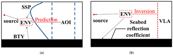
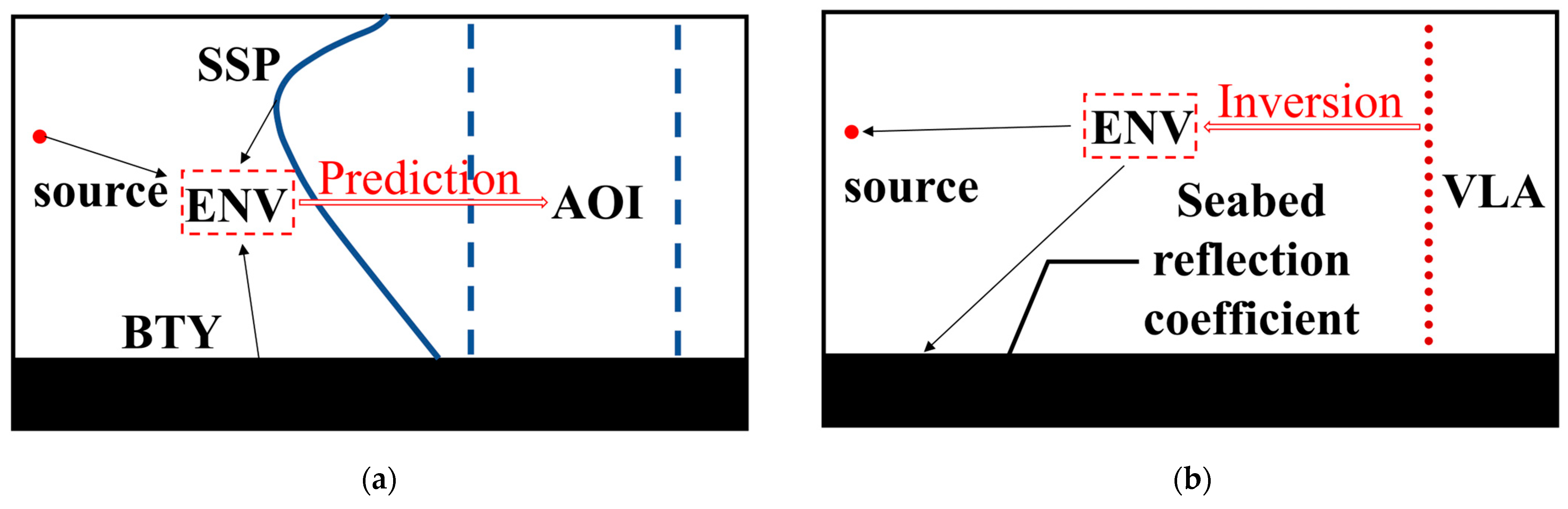
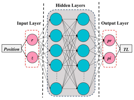
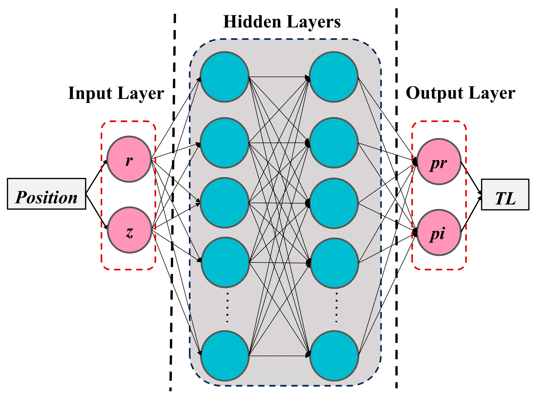
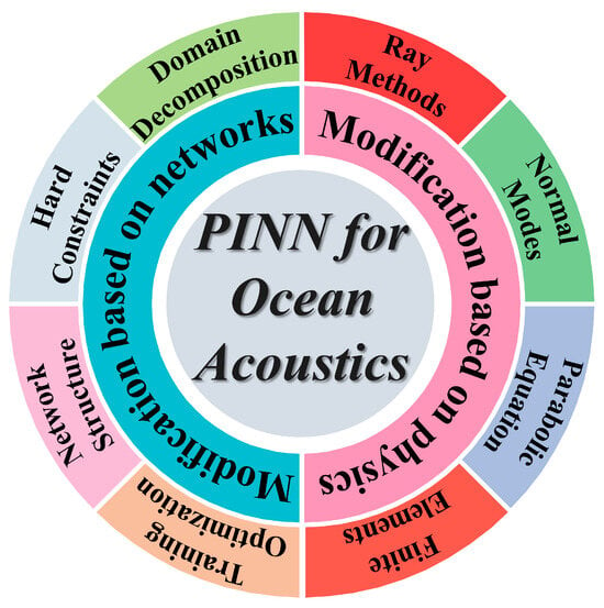
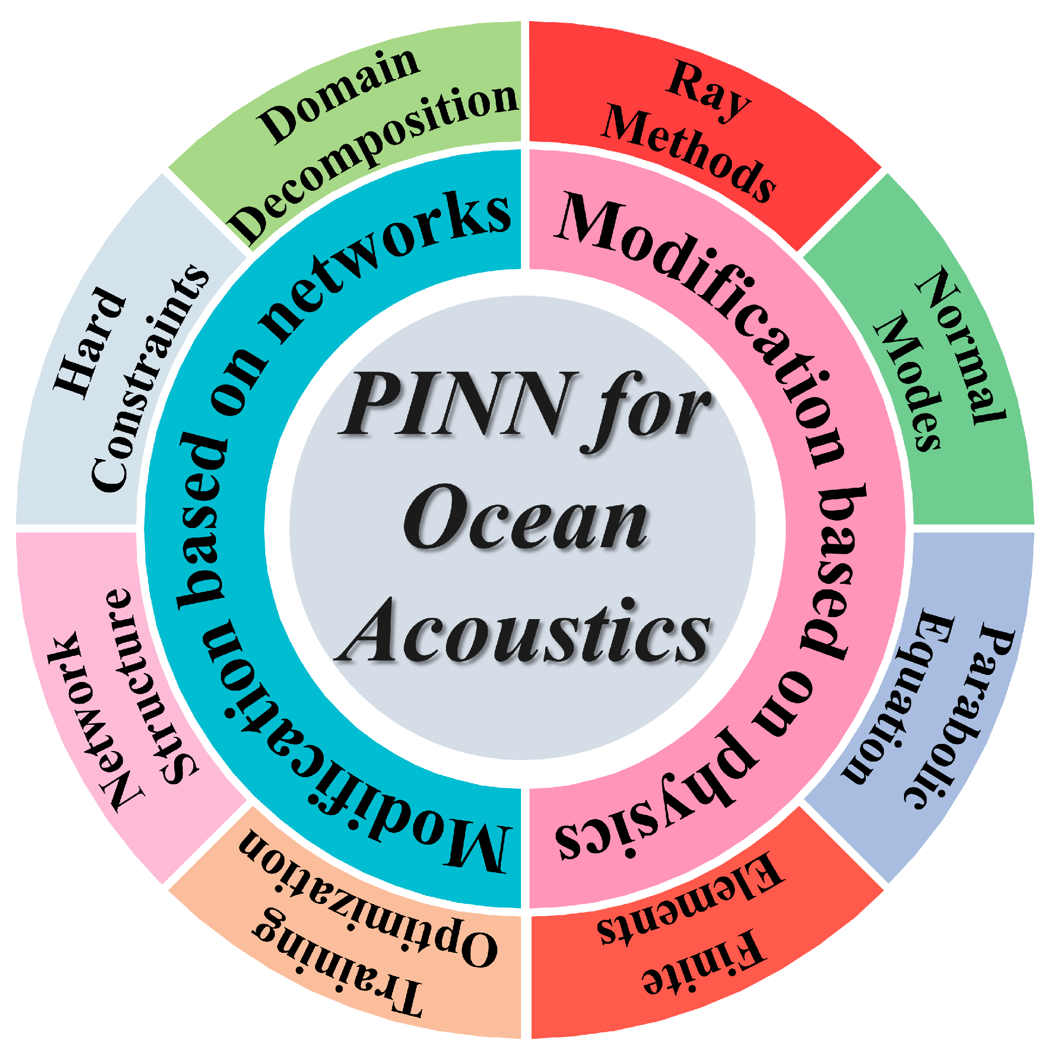
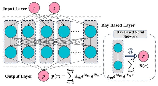
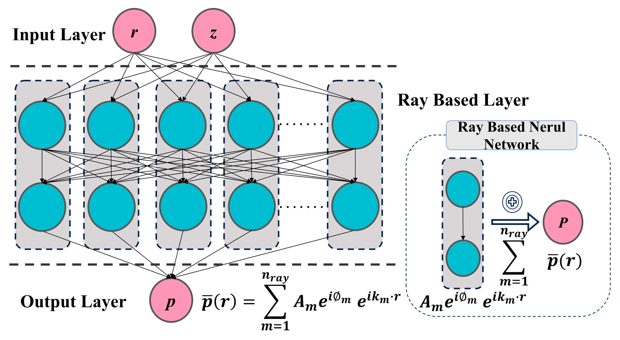
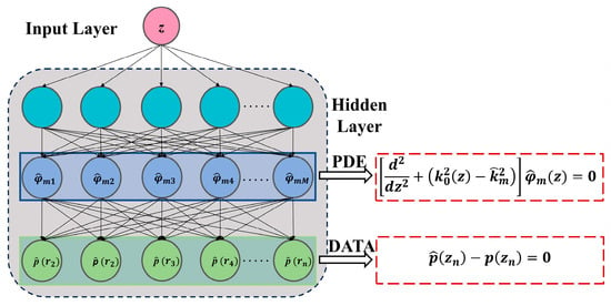
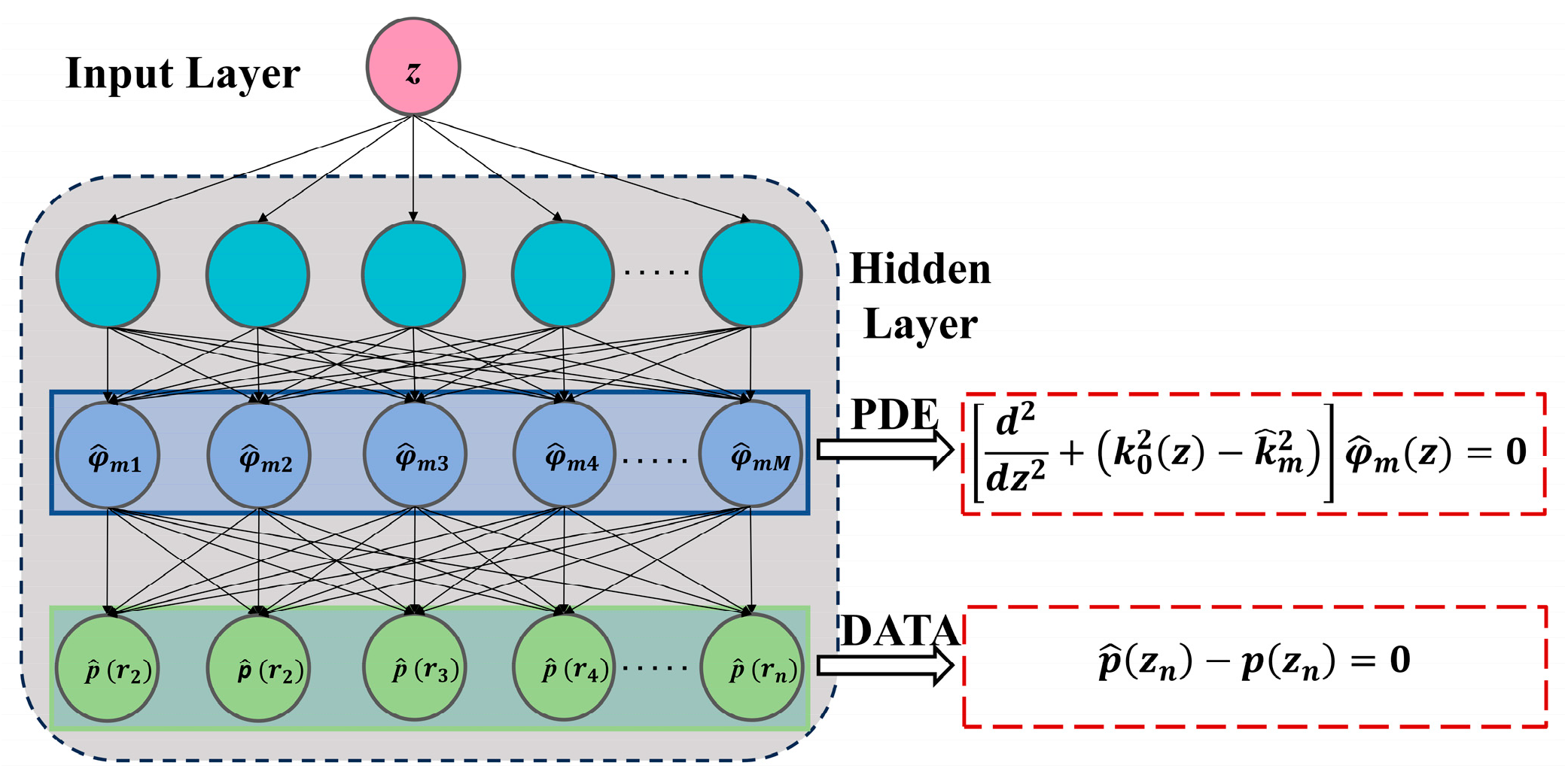
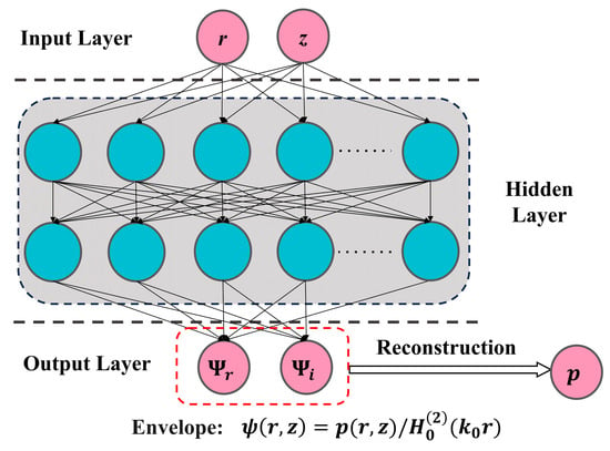
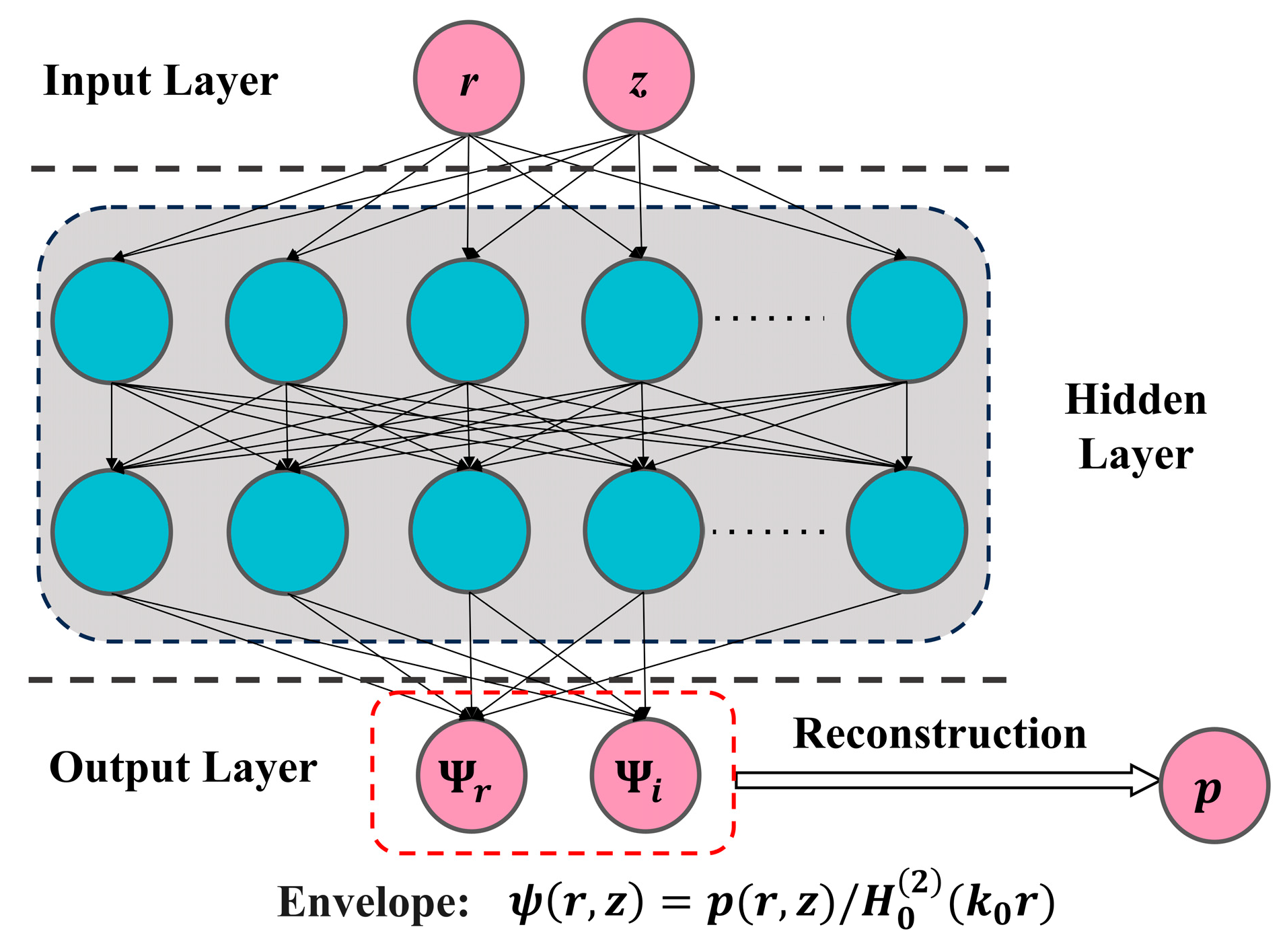
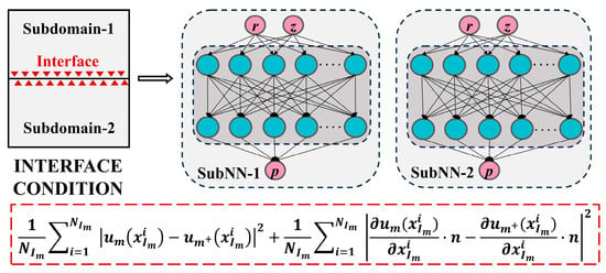
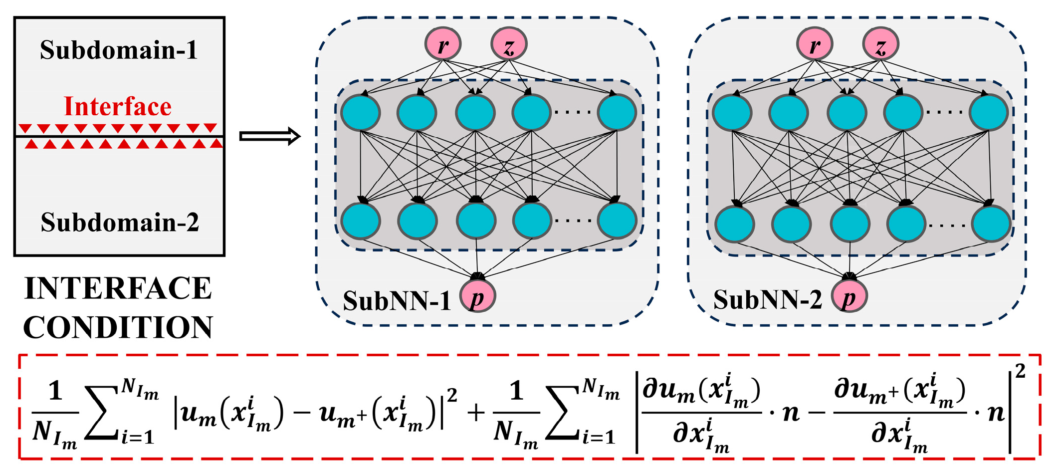
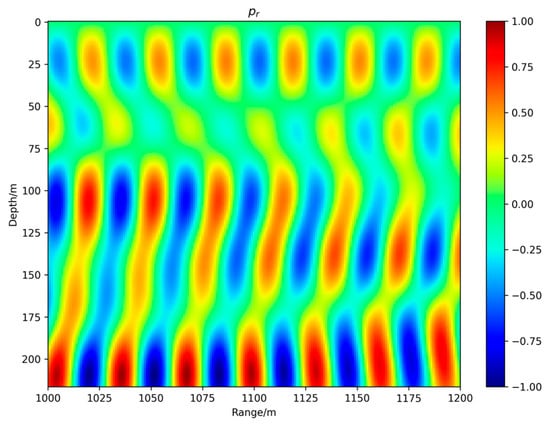
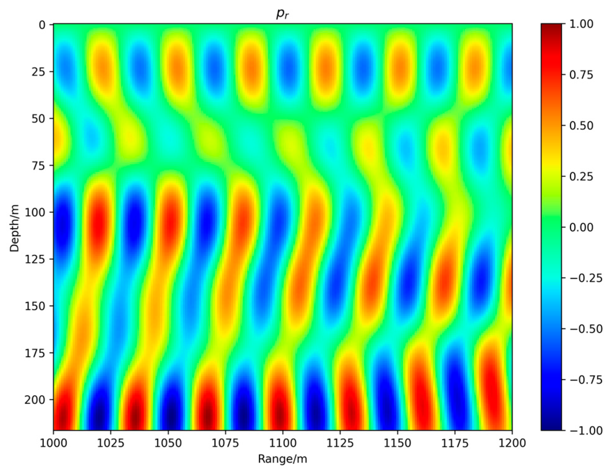
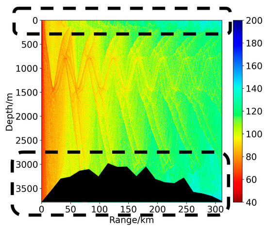
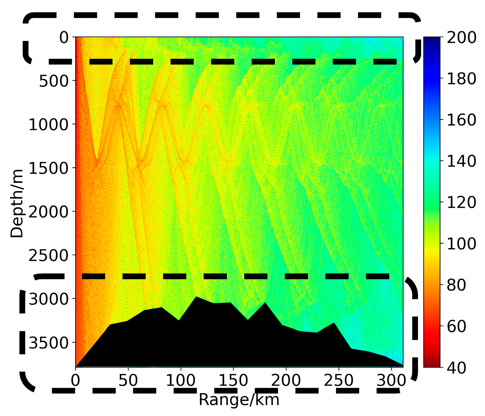
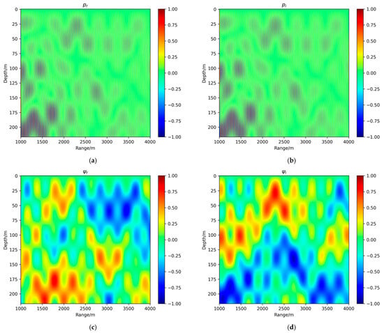
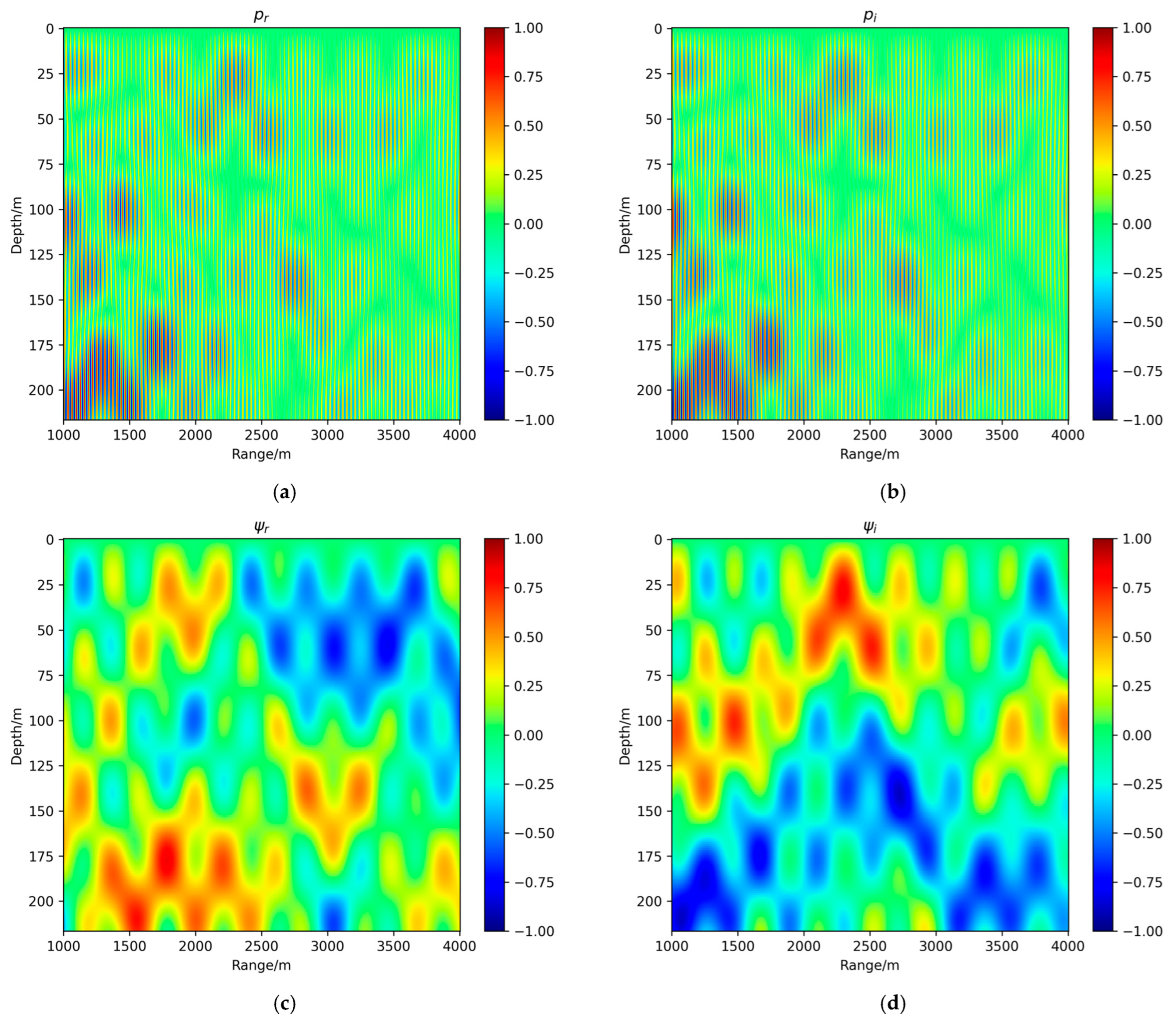
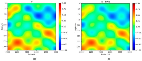
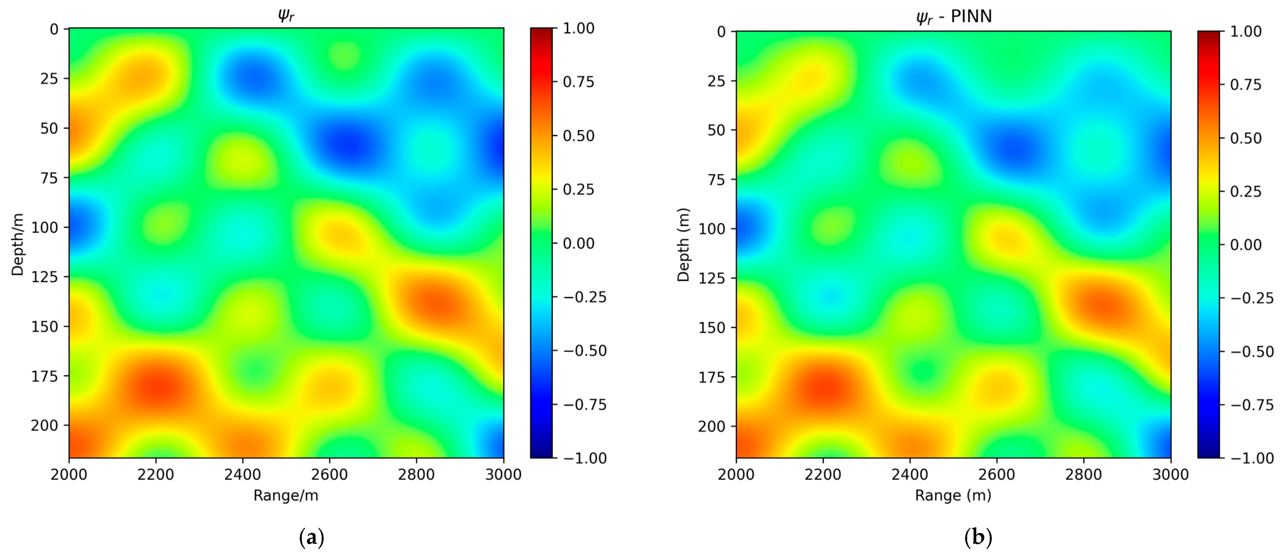
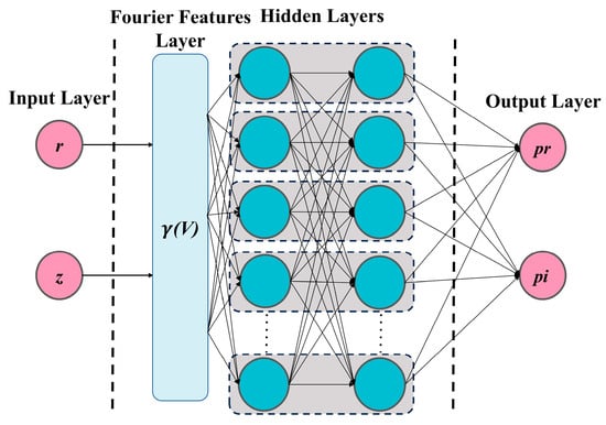
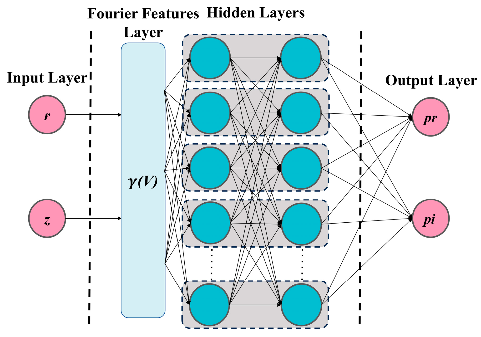
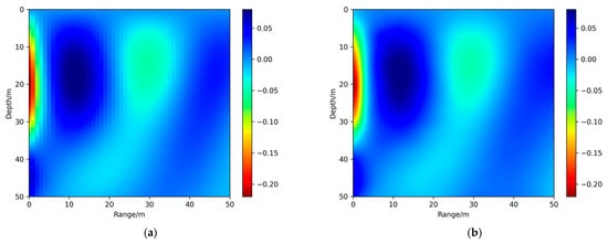
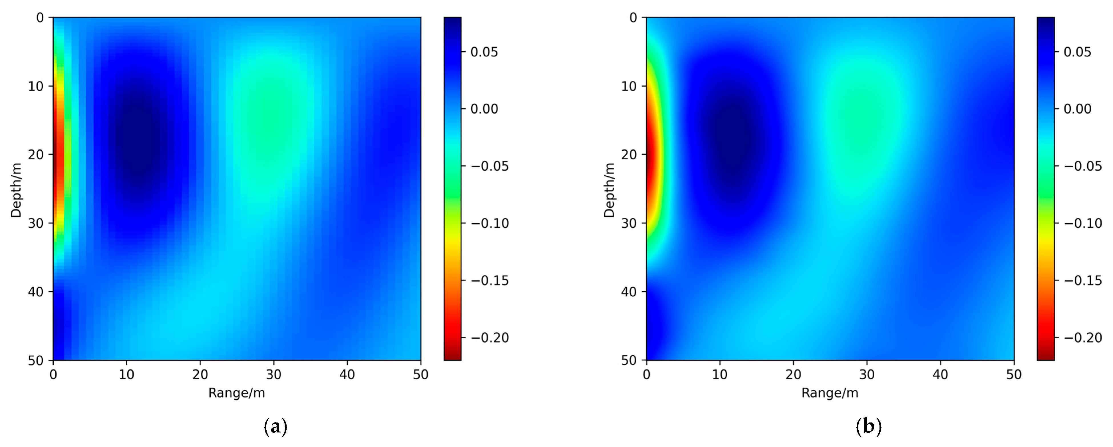

Disclaimer/Publisher’s Note: The statements, opinions and data contained in all publications are solely those of the individual author(s) and contributor(s) and not of MDPI and/or the editor(s). MDPI and/or the editor(s) disclaim responsibility for any injury to people or property resulting from any ideas, methods, instructions or products referred to in the content. |
© 2026 by the authors. Licensee MDPI, Basel, Switzerland. This article is an open access article distributed under the terms and conditions of the Creative Commons Attribution (CC BY) license.