


Abstract
Pitting corrosion is a localized degradation mechanism that can significantly affect the structural integrity of steel components while remaining difficult to detect and characterize using conventional monitoring approaches. This work investigates the use of pulse-echo ultrasound and data-driven signal analysis for the observability and characterization of localized pitting in low-carbon steel. The ultrasonic response of two 20 MHz single-element contact transducers was investigated through laboratory measurements on artificial pits and physics-based k-Wave simulations spanning a wider range of pit sizes and morphologies. The results show that localized pits modify the received signal through attenuation, scattering, waveform distortion, and the generation of secondary reflections, with the observed ultrasonic response strongly dependent on pit morphology and transducer aperture. A signal-processing and feature-extraction framework was developed to analyze these changes and to evaluate pit observability prior to characterization. Using pit-free measurements, observability limits were quantified with an autoencoder trained on signal descriptors, demonstrating that pit observability is influenced predominantly by pit geometry, normalized pit width, and pit volume rather than by depth alone. For signals exhibiting sufficiently observable and specular pit reflections, time-of-flight measurements enabled pit-depth estimation for defects deeper than 300 µm. To account for propagation-path distortions affecting pit-related echoes, an empirically derived cross-path delay compensation approach was developed using Random Forest models trained on synthetic signals, reducing systematic depth-estimation errors in the synthetic dataset and providing a physics-informed framework for future quantitative characterization studies. Additional Random Forest models employing waveform descriptors and reflection-amplitude indicators were used to assess pit morphology and acoustic surface specularity. The proposed framework was evaluated using laboratory measurements and through preliminary long-term monitoring of two pre-pitted specimens deployed in the HarshLab offshore environment. In these deployments, the methodology enabled simultaneous tracking of localized pit-wall evolution and overall backwall thickness changes from the same pulse-echo measurements, illustrating the potential of the approach for monitoring localized corrosion activity alongside generalized specimen wall loss.
1. Introduction
Pitting corrosion is one of the most critical degradation mechanisms affecting low-carbon structural steels operating in aggressive marine environments. In offshore wind turbine (OWT) support structures, steels such as S355 and S235 are continuously exposed to chloride-rich conditions that promote localized breakdown of the passive layer and the formation of corrosion pits [1,2]. Unlike uniform corrosion, pitting is highly localized and can cause significant structural degradation while affecting only a small fraction of the exposed surface. The impact of pitting on structural integrity is strongly influenced by the morphology and dimensions of the resulting cavities, which may act as severe stress concentrators and preferential initiation sites for fatigue cracks [3,4,5]. Consequently, the early detection, monitoring, and quantification of localized pitting are of considerable importance for the integrity management and lifetime assessment of offshore wind structures [6].
The need to improve structural reliability and reduce maintenance costs has motivated a transition from periodic inspections toward continuous structural health monitoring. A variety of non-destructive testing (NDT) techniques have been investigated for corrosion assessment, including visual inspection, radiography, thermography, acoustic emission, eddy-current testing, electrochemical methods, and ultrasonic testing [1,7,8,9,10]. Among these approaches, ultrasound is particularly attractive because it can provide volumetric information, operate non-invasively, and is compatible with permanently installed sensing systems.
Several ultrasonic techniques have been investigated for pitting detection, each addressing different aspects of the problem. Guided waves provide an effective means of large-area screening and can be combined with scattering, coda-wave, and nonlinear acoustic analyses to improve sensitivity to pitting corrosion [11,12,13]. Ultrasonic phased-array systems further enhance defect characterization in metallic components through beam steering and high-resolution imaging capabilities [14,15,16], and array-based ultrasonic imaging has also demonstrated effectiveness for the detection of internal defects in materials beyond steel, such as concrete [17]. For autonomous monitoring applications, however, pulse-echo ultrasound remains particularly attractive because it requires access to only the non-exposed side of the structure and can be implemented using compact, low-power sensors. Previous studies have shown that localized pits modify pulse-echo signals through attenuation, secondary reflections, scattering, and waveform distortions [18,19,20,21,22].
To enhance the detectability and characterization of these pit-induced signatures, recent studies have increasingly incorporated advanced signal-processing and learning-based approaches. Convolutional neural networks (CNNs) have been explored using timelapse representations of pulse-echo measurements to track pit evolution over time, demonstrating promising characterization capabilities for the specific drilled pit morphology considered in the study while relying on the availability of complete monitoring histories to construct the timelapse representation [20]. In parallel, autoencoder-based approaches have shown promise in suppressing noise and enhancing subtle defect signatures [21,23], while other deep-learning architectures have been investigated for feature extraction, localization, and characterization under challenging signal-to-noise conditions [24,25]. Machine-learning techniques have also been integrated into broader corrosion-monitoring frameworks, including multi-sensor approaches that combine field-signature measurements and ultrasonic thickness monitoring, with spatial voltage patterns from the field-signature measurements used to distinguish between shallow and deep pits [26]. Together, these developments highlight the growing potential of combining physics-based sensing with data-driven signal interpretation for localized corrosion assessment.
The increasing adoption of such machine-learning techniques in ultrasonic NDE has also motivated the use of synthetic and augmented datasets to overcome the scarcity of experimentally characterized defects. Recent reviews have summarized the growing role of physics-based simulations, data augmentation, and synthetic training datasets for defect detection and characterization tasks [27]. Likewise, simulation-to-experiment transfer has received increasing attention through domain-adaptation techniques that combine simulated and experimental datasets to improve model generalization and reduce the impact of domain mismatch [28].
Despite these advances, several challenges remain for the autonomous monitoring of localized pitting corrosion. Guided-wave approaches are well suited for large-area screening but often struggle to establish direct relationships between measured signals and the geometry of individual pits. Phased-array systems provide enhanced imaging capabilities but generally require more complex hardware, higher power consumption, and increased operational costs, limiting their suitability for distributed long-term monitoring networks. Pulse-echo methods offer a more deployable alternative, yet the ultrasonic signatures associated with small pits are often weak and strongly influenced by pit morphology, diffraction or scattering effects, transducer characteristics, and defect position within the sensing footprint.
Furthermore, existing studies have demonstrated their methods under specific experimental assumptions, such as relatively large defects, simplified drilled geometries, cylindrical or conical pit-like defects, multi-sensor corrosion-monitoring architectures, or approaches that require the complete monitoring history to infer pit depth, leaving open questions regarding the real-time detection and characterization of small, irregular pits under realistic corrosion conditions. Existing efforts have largely focused on defect detection, depth classification, corrosion-severity assessment, or the analysis of isolated ultrasonic indicators such as backwall amplitude variations, while comparatively less attention has been devoted to understanding when localized pits become observable from pulse-echo measurements, how observability depends on pit geometry, morphology, and sensing configuration, and which aspects of pit evolution can be reliably inferred from the ultrasonic response. In addition, the extent to which pulse-echo measurements can provide information beyond conventional wall-thickness monitoring, enabling the simultaneous tracking of specimen thickness and localized pitting activity, remains insufficiently explored. The limited availability of representative datasets and the incomplete understanding of how pit geometry influences ultrasonic observability also limit the development of robust machine-learning models and quantitative characterization methodologies for localized pitting corrosion.
This work addresses these challenges through a pulse-echo ultrasonic framework designed for long-term autonomous monitoring of localized corrosion in offshore environments, with periodic measurements enabling characterization of the current corrosion state. The proposed methodology extends previous developments in autonomous ultrasonic monitoring of uniform corrosion, where high-precision wall-thickness estimation was achieved through advanced signal-processing and time-of-flight (ToF) analysis techniques [29,30]. In contrast, the present study focuses on localized pitting corrosion, where scattering, diffraction, and localized reflections generate more complex ultrasonic patterns and where the observability of pit-induced signatures becomes a fundamental challenge.
Rather than aiming to provide full structural coverage, the proposed approach adopts a point-monitoring strategy in which compact sensing nodes are deployed at predefined areas of interest. The objective is to continuously monitor localized corrosion activity while maintaining low cost, low power consumption, and long-term deployability. To maximize sensitivity to small defects, the methodology prioritizes resolution over penetration capability. Since higher ultrasonic frequencies provide shorter wavelengths and improved axial resolution at the expense of increased attenuation, 20 MHz pulse-echo transducers are employed to enhance sensitivity to pit-induced reflections, scattering, and waveform distortions. Although direct installation on thick monopile structures is not feasible for these high-frequency sensors, the system is instead intended for deployment on dedicated steel coupons acting as pit-evolution indicators at strategically selected hot-spot locations, such as the splash zone, where localized corrosion is most severe.
The laboratory measurements are performed on specimens containing artificially introduced pre-pits designed to emulate corrosion cavities that form after the breakdown of the protective passive layer. These experiments are complemented by acoustic simulations performed with the k-Wave MATLAB toolbox [31], enabling the investigation of a much broader range of pit morphologies and dimensions than can be realized experimentally. The synthetic dataset is used to analyze the influence of pit geometry, pit size, and transducer footprint extent on ultrasonic observability, and to develop characterization models based on pulse-echo descriptors. To improve the realism of the simulated signals, domain-approximation techniques derived from defect-free experimental measurements are incorporated into the synthetic dataset, while pit-containing specimens are primarily employed to assess the ability of the framework to generalize beyond idealized simulated scenarios. A machine-learning framework is then developed to support pit observability assessment and characterization using temporal, spectral, and time-of-flight features extracted from ultrasonic signals. The proposed methodology introduces an empirical cross-path compensation model to improve pit-depth estimation from pit-wall-related echoes and investigates the use of pulse-echo descriptors as indicators of pit morphology, pit-wall specularity, and localized corrosion activity. Furthermore, in cases where pit-wall reflections remain sufficiently observable, the framework enables the simultaneous monitoring of pit-depth evolution and specimen-thickness evolution from the same pulse-echo measurement. While the results highlight the importance of simulation-to-experiment transferability and the need for more representative datasets of realistically corroded and accurately characterized pits, they establish a methodology for systematically investigating pit observability and characterization challenges in localized corrosion. Ultimately, this work provides a foundation for future autonomous ultrasonic monitoring nodes capable of intelligent pit observability assessment and characterization during long-term offshore deployments.
The remainder of this paper is organized as follows. Section 2 describes the proposed methodology, including the ultrasonic monitoring system, the experimental specimens and measurements, the k-Wave numerical simulations, the signal-processing pipeline, the feature-extraction procedure, the domain-transferability analysis, the cross-path propagation compensation for pit-depth estimation, and the machine-learning framework developed for pit observability assessment and characterization. Section 3 presents the experimental and numerical results along with the corresponding discussion, including simulated signal characteristics, pit observability studies, descriptor transferability analysis, pit characterization results, and long-term monitoring experiments. Finally, Section 4 summarizes the conclusions and outlines directions for future work.
2. Materials and Methods
This section describes the methodology followed in this work for the detection and characterization of localized pitting corrosion using pulse-echo ultrasound. An overview of the methodology is presented in Figure 1. The workflow is organized into three main stages: data acquisition, signal processing and feature extraction, and a machine-learning-based analysis. Data acquisition combines laboratory measurements, long-term monitoring experiments, and three-dimensional k-Wave simulations to obtain representative ultrasonic responses from both pitted and non-pitted conditions. The acquired signals are subsequently processed to isolate relevant echoes and extract temporal, spectral, and time-of-flight features associated with localized pits. These features are then used within a machine-learning workflow that includes pit observability analysis and pit characterization, providing estimates of pit depth, shape, and relative width while supporting long-term autonomous pitting corrosion monitoring.
Figure 1.
Methodology used to develop the proposed data-driven framework for pitting corrosion monitoring using pulse-echo ultrasound.
2.1. Data Acquisition
This stage focuses on the generation of ultrasonic datasets used throughout the study. Laboratory measurements, long-term field monitoring experiments, and physics-based numerical simulations were combined to obtain representative ultrasonic responses from both pitted and non-pitted conditions. Throughout this work, the transducer is assumed to be centered over the pit location, so that the measured signal depends primarily on the pit characteristics rather than on lateral positioning within the ultrasonic beam. The resulting dataset was subsequently used for signal analysis, feature extraction, and machine-learning models development.
2.1.1. Experimental Measurements
The monitoring approach is based on a pulse-echo ultrasonic configuration using a single-element transducer coupled to the rear surface of the inspected steel component. Longitudinal waves are introduced into the material, and reflections from localized pits and the backwall are analyzed to assess corrosion damage. In laboratory experiments, coupling gel is used to ensure proper acoustic contact, while in long-term monitoring the transducer is permanently glued.
The measurements are performed using the smart ultrasonic corrosion monitoring system presented in [29]. Data acquisition can be initiated via a PC-based executable or configured for automated periodic operation. The acquisition procedure follows the pulse-echo implementation described therein. Signals are recorded using a pulse-echo configuration with an analogue-to-digital converter (ADC) sampling at 125 MHz, corresponding to a temporal resolution of 8 ns per sample.
Artificial pitting defects were introduced into S235 low-carbon steel samples provided by C-Cube International (Delft, The Netherlands) and S355 low-carbon steel samples provided by Sirris (Brussels, Belgium) to emulate localized corrosion cavities. Two defect types were considered: cylindrical machined pits in the S235 specimens and mechanically hammered pits in the S355 specimens. The investigated defects covered a range of geometries representative of early-stage localized corrosion, with diameters up to 3 mm and depths up to 1.2 mm. This study employed two 20 MHz contact ultrasonic transducers acquired from Evident Scientific (Waltham, MA, USA), selected to provide high axial resolution and aperture sizes comparable to the pit dimensions:
- V116: 20 MHz transducer with a 3.2 mm nominal element diameter.
- V212: 20 MHz transducer with a 6.4 mm nominal element diameter and a 4.336 s delay line.
The V116 and V212 transducers correspond to commercial 1/8 in. (3.175 mm) and 1/4 in. (6.35 mm) element specifications, respectively. Nominal rounded metric values (3.2 mm and 6.4 mm) are used consistently throughout all simulation setups and analytical formulations.
The longitudinal wave velocity in the S235 specimens was experimentally calibrated using a reference sample. Measurements were performed at six locations, with five repeated measurements acquired at each location. For every measurement, five consecutive ultrasonic acquisitions were recorded and used to estimate the time-of-flight. Thickness measurements (d) were obtained measuring the same six spots with a digital micrometer, and the longitudinal speed of sound was calculated according to . The resulting average longitudinal wave velocity was () m/s. For the S355 specimens, the value of 5950 m/s reported in [29] was adopted.
Laboratory measurements were performed on the artificial pit specimens under controlled conditions. Additional measurements were also conducted on hammered pre-pitted S355 samples immersed in salt water to increase the dataset of pit conditions under accelerated laboratory corrosion. Long-term monitoring of corrosion evolution was carried out using autonomous sensing nodes on two 5 mm thick S235 specimens with cylindrical pre-pits, deployed at the floating test site HarshLab [32], located off the Basque Country coast. The first specimen contained a 0.7 mm deep, 2 mm diameter pre-pit and was monitored using the V212 transducer from September 2025 to April 2026, whereas the second contained a 0.5 mm deep, 1 mm diameter pre-pit and was monitored using the V116 transducer from April 2026 (ongoing; data analyzed in this work cover measurements through July). The autonomous sensor nodes operated periodically, collecting measurements every six hours.
2.1.2. Synthetic Signal Generation Using k-Wave Simulations
Three-dimensional numerical simulations were performed using the k-Wave toolbox to generate synthetic pulse-echo ultrasonic signals representative of corrosion pits. The k-Wave toolbox solves coupled first-order wave equations using a k-space pseudospectral method on a spatially and temporally staggered grid, utilizing its elastodynamic extension to model full elastic wave propagation within the solid specimen [33]. For pit-like volumetric defects, the two-dimensional formulation previously used for layered media signal generation in [34] was extended to a fully three-dimensional representation. The numerical model reproduced the experimental inspection configuration while enabling systematic variation of pit geometry beyond what could be practically manufactured or measured experimentally. The resulting synthetic dataset was used to investigate pit observability, analyze the effects of pit geometry and sensing configuration, support descriptor-based characterization, and evaluate transferability under experimental conditions.
A nominal steel plate thickness of was selected for the primary simulation dataset, as it provides sufficient path length to ensure complete temporal separation between successive round-trip echoes, preventing reflections from adjacent passes from overlapping while maintaining computational efficiency. A subset of simulations was also conducted at to incorporate thickness-dependent variations in the pit-related ToF indicators. A three-dimensional Cartesian computational domain was defined to represent a steel plate coupled to a medium on one side and exposed to air on the opposite side. Ten grid points of perfectly matched layers (PML) were applied inside all boundaries to minimize artificial reflections at the domain edges [33]. For the and steel specimens, total grid dimensions (including PML) were nodes (active physical domain of nodes spanning ) and nodes (active physical domain of nodes spanning ), respectively. Total grid sizes were chosen with small prime factors (≤5) for optimal Fast Fourier Transform execution. Dividing active physical dimensions by interior node counts (excluding PML) yielded spatial discretization steps of ( case) and ( case) along the propagation axis, and laterally. These spatial grid steps satisfy the Nyquist criterion of at least two points per acoustic wavelength required by k-Wave’s Fourier pseudo-spectral operator for longitudinal wave propagation in steel (, at 20 MHz). Specifically, this resolution yields over 9 points per wavelength along the main propagation axis () and ≥3.2 points per wavelength laterally (), satisfying k-Wave’s recommended 3–4 points per wavelength guideline for heterogeneous media, and ensuring minimal numerical spatial dispersion while balancing 3D computational cost and spatial representation of the pit geometries. Under the Rayleigh scattering regime, the sub-wavelength stair-casing steps introduced by the discretization are assumed to have minimal influence on specular reflections, primary echo amplitudes, and coherent mode conversion under the evaluated configurations. The propagation medium consisted of three materials representing an effective transducer–couplant layer, the steel specimen, and the surrounding air. Their acoustic properties, along with justifications for specific physical and numerical parameter choices, are detailed in Table A1 of Appendix A.
Localized pits were defined by creating air cavities within the steel medium. Four defect geometries representative of localized corrosion were considered: cylindrical, truncated-conical, Gaussian, and elliptical pits. The cylindrical and truncated-conical cases define a continuous family in which the shape transitions from a conical pit to a flat-bottom cylindrical pit as the inner diameter increases from zero. Gaussian and elliptical geometries were included alongside this family to represent a broader range of pit-like cavities that may occur on steel surfaces under different corrosion conditions. Each pit was parameterized by its depth d, surface outer diameter w, and an offset parameter o accounting for possible asymmetric material removal in the axial direction. Overall, the selected geometries and parameterization were designed to emulate defect variability. While naturally occurring marine corrosion often produces irregular, asymmetric, or multi-pitted morphology patterns, the single and symmetric defect configurations evaluated in this work serve as a controlled baseline. This idealization isolates the fundamental physical relationships governing acoustic wave interaction, cross-path ToF delays, and echo attenuation as a function of single pit dimensions, avoiding confounding interference from adjacent pit scattering before extending the methodology to complex, unstructured corrosion states. Simulated pit depths ranged from 0.1 to 1.0 mm. The maximum surface diameter was constrained by the transducer aperture to ensure physically consistent interaction between the ultrasonic field and the defect. Specifically, pit diameters were limited to half the transducer aperture diameter (), resulting in ranges of 0.2–1.6 mm for the V116 transducer (3.2 mm aperture) and 0.4–3.2 mm for the V212 transducer (6.4 mm aperture). In addition to ideal smooth surfaces, backwall roughness was introduced to emulate uniform corrosion-induced surface degradation (mathematically formulated in Appendix A). Both smooth and rough backwall conditions were equally represented in the simulated dataset. Representative computational domains illustrating the different simulated pit geometries and backwall conditions are shown in Figure 2.
Figure 2.
Representative computational domains employed in the k-Wave simulations: (a,e) cylindrical, (b,f) truncated cone, (c,g) semi-ellipsoidal, and (d,h) Gaussian pit geometries. The first row (a–d) corresponds to smooth backwall conditions, whereas the second row (e–h) includes backwall roughness mimicking uniform corrosion. All examples correspond to pits with a depth of and a surface diameter of , allowing direct comparison of the different pit geometries and backwall conditions.
Rather than using an ideal analytical pulse, the excitation waveform was derived directly from experimental measurements. For each transducer (V116 and V212), a normalized backwall echo acquired from a defect-free steel specimen was used as an approximation of the incident ultrasonic pulse. The corresponding waveform was interpolated to the temporal discretization of the numerical model and used as the source excitation. The ultrasonic source was modelled as a circular piston reproducing the physical aperture of each experimental transducer. A Gaussian weighting was applied across the active element as an effective source apodization to improve the agreement between simulated and experimentally measured echoes from specimens containing pit defects. The Gaussian standard deviation was defined as , where R is the transducer radius and is a dimensionless scaling factor controlling the degree of source apodization. The parameter was calibrated by maximizing the normalized cross-correlation (NCC) between simulated and experimentally measured echoes from the two samples that were subsequently deployed for long-term exposure at HarshLab. The calibration yielded for the V116 transducer and for the V212 transducer. These values should therefore be interpreted as effective modeling parameters rather than direct physical properties of the transducers. Figure 3 shows the simulated and experimental waveforms obtained with the calibrated source model. The corresponding NCC values were 0.925 and 0.959 for Echo 1 and Echo 2, respectively, for the first sample, and 0.981 and 0.985 for Echo 1 and Echo 2, respectively, for the second sample, indicating close agreement between the simulated and experimental waveforms. The remaining minor discrepancies are attributed to the finite computational grid resolution and the modeling approximations adopted to reproduce the experimental conditions.
Figure 3.
Comparison of simulated and experimentally measured Echo 1 and Echo 2 signals for the two cylindrical pre-pits in 5 mm thick steel specimens used to calibrate the source model, obtained after optimization of the beam apodization parameter: (a) 0.5 mm deep, 1 mm diameter pre-pit (V116 transducer); and (b) 0.7 mm deep, 2 mm diameter pre-pit (V212 transducer). The simulated echoes were interpolated and temporally aligned before computing the normalized cross-correlation (NCC), whose value is reported in each subplot.
Synthetic signals were generated to cover the range of pit geometries and dimensions described previously for both transducer configurations. For each simulation, the A-scan signal was obtained by spatially averaging the acoustic pressure across the active receiver surface elements and subsequently downsampled from approximately 3 GHz to 125 MHz to match the sampling frequency of the experimental acquisition system. The simulated dataset included both pitted and non-pitted specimens: a larger number of pitted cases was generated to provide sufficient variability for pit characterization, whereas a smaller set of non-pitted signals was included for pit observability analysis. Simulations were performed under both smooth and rough backwall conditions. Since grid discretization introduces small deviations from the nominal pit geometry, the effective pit dimensions were recomputed after discretization and stored together with each simulated signal. These recomputed dimensions were subsequently used as ground-truth labels in all analyses, thereby accounting for discretization-induced deviations from the nominal geometry and preventing artificial ToF shifts in target labels.
To reduce discrepancies between simulated and experimental ultrasonic responses, a transfer-function-based spectral augmentation strategy was introduced as a domain adaptation effort to account for variability in the reference backwall echo used to define the simulation excitation (see Appendix A for mathematical derivation). Using a regularized inverse filter, spectral mapping functions were estimated from experimentally measured defect-free backwall echoes to quantify variations in coupling, transducer response, and acquisition electronics without requiring computationally expensive re-simulations. To incorporate this variability into the dataset, three transfer functions were randomly sampled from the transducer-specific database and applied to the spectrum of each simulated signal. This spectral augmentation approach introduced realistic acquisition-chain perturbations, increasing the dataset size by a factor of three to yield nearly 50,000 synthetic signals, of which 12% correspond to defect-free cases.
2.2. Signal Processing and Feature Extraction
The acquired ultrasonic signals were processed with MATLAB R2024a to enhance defect-related information and reduce the influence of measurement noise. Following signal conditioning, a set of temporal, spectral, and time-of-flight features was extracted to characterize waveform modifications associated with localized pitting corrosion. Additional analyses were performed to compensate for cross-path propagation effects affecting depth-related ToF measurements.
2.2.1. Signal Processing
All experimental and synthetic A-scan signals were processed using a common signal processing pipeline derived from the methodology previously proposed for uniform corrosion monitoring [30] and adapted here for localized pit characterization. Applying the same processing chain to all experimental measurements (from both the V116 and V212 transducers) and to all synthetic signals, ensured methodological consistency across the entire dataset and between the experimental measurements, numerical simulations, and the reference echoes used to define the simulation excitation. The processing workflow consisted of four main stages:
- 1.
- Band-pass filtering.
- 2.
- Wavelet-based denoising.
- 3.
- Echo detection and windowing.
- 4.
- Propagation medium impulse response estimation.
First, the acquisition system dead zone was removed. The resulting signals were then filtered using a zero-phase finite impulse response (FIR) band-pass filter, designed with a Hanning window, 115 coefficients, and a passband extending from 3 to 28 MHz. Its primary purpose was to suppress the low-frequency components associated with the transient response of the transducer and acquisition system (more pronounced for the V116 transducer and substantially reduced for the V212 transducer due to the delay line), together with high-frequency electronic noise outside the useful ultrasonic bandwidth. However, the dominant source of noise in the inspected specimens is grain scattering, whose spectral content overlaps that of the pit echoes. Consequently, the band-pass filter cannot provide significant additional noise reduction without also attenuating defect-related information.
To further improve the signal-to-noise ratio while preserving the transient characteristics of the ultrasonic echoes, the filtered signal was subsequently denoised using the maximal overlap discrete wavelet transform (MODWT) with a Symlet-4 mother wavelet and four decomposition levels. Soft thresholding was applied to the detail coefficients at the first three decomposition levels, while the fourth level was left unchanged before signal reconstruction. Unlike conventional frequency-domain filtering, wavelet denoising exploits the joint time-frequency representation of the signal, enabling selective attenuation of grain-scattering noise while preserving localized echo features associated with pit reflections.
An analytic envelope was then computed to facilitate echo localization. The first two longitudinal backwall echoes were identified by searching for the strongest envelope maxima satisfying the expected separation imposed by specimen thickness. Only the first two echoes were considered, as they provide the highest signal-to-noise ratio and most reliable information for pit analysis. In higher-order echoes, cumulative attenuation progressively reduces signal amplitude, while multiple reflections and increasingly complex propagation paths produce more intricate waveforms that complicate the identification and interpretation of pit-related reflections. Signals not fulfilling minimum quality criteria, including insufficient signal-to-noise contrast, missing echoes, saturated acquisitions, or inconsistent echo spacing, were discarded from further analysis.
Once the envelope maximum of each backwall echo had been identified, a fixed analysis window was extracted using predefined offsets relative to the detected maximum. These parameters were optimized for the 3 mm and 5 mm thick specimens to capture the complete backwall reflection together with any associated pit-related reflections while avoiding overlap with adjacent round-trip echoes. This windowing assumes that the information relevant for subsequent analysis is confined to these temporal intervals, whereas signal components outside the selected windows are treated as undesired noise. Finally, a Tukey window with a tapering parameter of 0.1 was applied to each extracted echo to smoothly attenuate the window edges, further suppressing residual out-of-window contributions without distorting the waveform within the region of interest and improving the numerical stability of the subsequent spectral analysis.
Following echo extraction, the propagation medium impulse response between the first and second backwall echoes was computed using the frequency-domain deconvolution procedure presented in our previous work [34]. This representation largely removes the influence of the excitation waveform and isolates the propagation characteristics of the inspected specimen, providing an alternative signal representation for subsequent analysis. Figure 4 illustrates a representative raw experimental signal after sensor dead-zone removal together with the corresponding processed signal after band-pass filtering, wavelet denoising, and automatic echo segmentation.
Figure 4.
Ultrasonic A-scan signals acquired using the V212 transducer from a 5 mm thick specimen containing a cylindrical pit with a diameter of 2 mm and a depth of 0.7 mm: (a) raw signal after dead-zone removal; and (b) band-pass filtered and wavelet-denoised signal with windowed echo regions highlighted for subsequent analysis. The dominant sub-echo in each echo region corresponds to the backwall reflection, whereas the weaker sub-echoes preceding the dominant one correspond to reflections from the pit.
2.2.2. Feature Extraction
Following signal processing, a set of descriptors was extracted from the isolated echoes to characterize waveform distortions associated with localized pitting. A first group comprised global temporal and spectral descriptors, including metrics such as signal-to-noise ratio (SNR), inter-echo relative energy decay, statistical moments (skewness and kurtosis), crest factor, energy-based temporal echo width, spectral centroid, and bandwidth. To specifically capture pulse deformations induced by pitting corrosion, three additional energy-based descriptors were formulated and included in the descriptor set: the Coherent Energy Ratio (CER), Secondary Energy Ratio (SER), and Energy-Weighted Asymmetry (EWA). Graphical representations and definitions of these specialized energy descriptors are provided in Appendix B. From a wave propagation standpoint, both standard and energy-based descriptors respond to physical phenomena such as edge diffraction, intra-pulse phase interference, and multi-path scattering at the defect boundary. Because these acoustic mechanisms interact non-linearly with pit depth, wall slope, and surface aperture, individual features may not exhibit direct one-to-one relationships with isolated geometric parameters. Nevertheless, the complete descriptor set jointly captures changes in echo amplitude, symmetry, duration, and frequency distribution, remaining informative even when a distinct pit reflection cannot be resolved (e.g., due to temporal overlap with the backwall echo or diffuse scattering). Multivariate models can thus leverage these combined variations to achieve robust geometric estimations despite complex, coupled wave distortions. Additionally, the time-of-flight (ToF) between Echo 1 and Echo 2 was estimated from the parabolically interpolated peak of their cross-correlation. Assuming that delays introduced by pit reflections within either echo are negligible, this echo-to-echo ToF directly corresponds to the remaining backwall thickness.
A second group of descriptors relied on the identification of pit-related reflections and therefore could only be extracted when these reflections were observable. A dedicated peak analysis algorithm was applied to the first echo, the second echo, and the impulse response. The algorithm identifies the dominant backwall reflection together with a preceding pit-related reflection whenever both can be reliably separated. For Echo 1 and Echo 2, peak detection was performed after cross-correlating each isolated echo with a bipolar rectangular reference pulse matched to the characteristic signal period of () approximately. This reference pulse acts as a computationally efficient matched filter that suppresses out-of-band noise and stabilizes the correlation envelope. The resulting peak locations were refined using parabolic interpolation, and the pit-to-backwall ToF was computed as the temporal distance between the interpolated pit and backwall correlation maxima. For the impulse response, the ToF was evaluated directly on the deconvolved waveform peaks following parabolic interpolation. Corresponding amplitude ratios were subsequently extracted to characterize the redistribution of acoustic energy caused by pit-induced scattering. The extracted peak-based descriptors include:
- Pit-to-backwall ToF and corresponding amplitude ratio estimated from the first-echo waveform .
- Pit-to-backwall ToF and corresponding amplitude ratio estimated from the second-echo waveform .
- Pit-to-backwall ToF and corresponding amplitude ratio estimated from the deconvolved impulse response signal .
These peak-based descriptors provide a more direct characterization of the pit geometry. In particular, the pit-to-backwall time-of-flight is directly related to the pit depth. In long-term monitoring campaigns, ToF metrics were compensated for temperature dilation relative to the lab temperature by using temperature readings from the sensor node and applying the calibrated value and the method detailed in [30]. Meanwhile, the relative amplitudes of the pit and backwall reflections are influenced by the pit reflectivity, which depends on its radial extent, geometry, and orientation relative to the incident ultrasonic field. Consequently, whenever pit-related reflections can be reliably separated from the backwall echo, these descriptors provide physically interpretable information for pit characterization. When a distinct pit reflection is not observable, the global temporal and spectral descriptors remain applicable and provide complementary information for pit observability assessment and approximate geometry estimation.
2.2.3. Time-of-Flight Analysis and Cross-Path Compensation
The ToF metric extracted from the first echo exhibits a direct relationship with . The corresponding metrics extracted from the second echo are affected by cross-path propagation effects that introduce systematic delays relative to the true pit depth. Because the deconvolution response is computed from the first and second backwall echoes, its ToF metrics are likewise influenced by these delays and therefore exhibit a similar systematic offset. These effects would be negligible if the pit depth was much smaller than the sample thickness (); however, in the coupons considered in this work (3 mm and 5 mm), , while smaller than , is not small enough relative to it for this approximation to hold. To compensate for these effects, time-of-flight descriptors extracted from synthetic pit signals with known depths were used to fit compensation models accounting for the additional propagation path introduced by pit reflections. The availability of multiple compensated ToF metrics provides independent estimates of pit depth and enables depth quantification even when only one of the possible pit-related reflections is detected.
Figure 5 illustrates the ultrasonic propagation paths considered in the presence of a pit, including the direct and cross-path contributions. Two reflectors are considered: the pit-wall () and steel backwall (), both representing steel-to-air acoustic transitions with same-sign pressure amplitudes and . The direct echo paths from each reflector are:
Defining the time-of-flight difference (so that ), the first received round-trip echo is expressed as:
where and relate directly to pit depth and total thickness via the speed of sound in steel :
As only the pit-wall term depends on , measuring peak separation in directly yields the pit depth .
Figure 5.
Ultrasonic wave propagation paths in steel in the presence of a pit.
Because the pit-wall is a finite reflector, part of the transducer beam rebounding from the rearside surface (scaled by attenuation ) illuminates the neighboring reflector, giving rise to cross-path contributions in the second round-trip echo ():
where and are effective cross-path amplitudes, and , are excess propagation delays relative to direct paths. The complete geometric derivation of and and their small-angle trigonometric approximations are detailed in Appendix C.
Since and diverge from one another as grows, the two cross-path contributions do not, in general, arrive at the exact same instant. For real, band-limited echoes of finite duration, this arrival offset may cause partial constructive or destructive overlap between wavelets, distorting peak shape and amplitude. Non-ideal perturbations (such as pit-wall curvature, non-specular reflection, or diffraction) further affect cross-path timing and amplitude in ways not captured analytically. To compensate for these effects without overparameterizing the model, a single effective delay
is characterized empirically from synthetic signals and used for compensation. This deliberate simplification treats both cross-paths as fully coincident and summed into a single doubled contribution at that time position.
Combining the direct and cross-path terms under the single effective delay , and substituting , the second received round-trip echo is:
The first term () is attenuated by squaring and typically untrackable in practice. Pit depth analysis in therefore relies on peak separation between the coincident cross-path term and the backwall double-bounce term, compensating for . The delta representation of the reflections contributing to each round-trip echo is shown in Figure 6.
Figure 6.
Simplified echo timing diagram showing the reflected contributions in and , where vertical arrows represent ideal Dirac delta impulses.
Having independent depth estimates from and ensures robust characterization when one echo fails to yield a trackable peak. While the pit locally delays the backwall arrival time across the transducer aperture, as observed in the k-Wave simulated B-scans in this study and previously reported by Wangensteen et al. [20], this spatial variation is smoothed out when the response is averaged over the transducer aperture to form the A-scan, and is not separately resolvable in the resulting for the transducers and pit dimensions considered in this work. The backwall ToF, and correspondingly via Equation (3), can therefore be taken as an estimate of generalized wall thinning. Tracking over time, alongside , allows the evolution of the pit to be monitored separately from, and compared against, generalized corrosion affecting the sample’s overall thickness.
2.3. Machine Learning Workflow
The extracted ultrasonic descriptors were used to develop a machine-learning methodology for pit observability analysis and characterization. The workflow combines synthetic datasets generated using the proposed three-dimensional simulation framework with experimental measurements acquired from laboratory specimens and long-term monitoring campaigns. Synthetic data provide extensive coverage of pit geometries and dimensions under controlled conditions, whereas experimental data incorporate realistic acquisition variability. The complete framework was implemented in Python 3.9.18.
2.3.1. Domain Transferability and Feature Selection
Although the numerical simulations reproduce the main physical mechanisms of ultrasonic wave propagation—and even after applying the spectral augmentation filters described in Appendix A to the 1D synthetic signals to reduce the domain gap—the simulated outputs cannot capture all the variability present in experimental measurements. These discrepancies might arise from physical non-idealities (such as instrumentation effects, electronic noise, couplant thickness variations, and grain scattering) as well as morphological differences. While synthetic pits cover a broad parametric range of sizes and shapes under ideal centered conditions, some experimental specimens exhibit localized pitting roughness around the defects from salt-water exposure that are not fully captured by synthetic backwall roughness models. Consequently, the transferability of the extracted descriptors between the synthetic and experimental datasets was evaluated before training the machine-learning models.
The signals underwent the processing and feature extraction described in Section 2.2, yielding an initial set of 34 ultrasonic descriptors per sample, corresponding exclusively to the first group of non-distance-based descriptors. These descriptors remain informative independently of whether the pit reflection can be identified as a distinct echo, making them suitable for the observability stage.
Some descriptors provide almost the same information. To avoid redundancy, pairs of descriptors with a Spearman correlation coefficient greater than were considered equivalent, and one descriptor from each pair was removed. The remaining descriptors were then evaluated for their transferability between the synthetic and experimental datasets.
The transferability of each descriptor was quantified using the domain-AUC criterion, based on the proxy -distance framework proposed by Ben-David et al. [35]. For each descriptor separately, a rank-based classifier (equivalent to the Mann–Whitney U statistic) attempted to distinguish synthetic from experimental samples using only that descriptor. A domain-AUC close to 0.5 indicates that the descriptor has a similar distribution in both datasets and is therefore highly transferable, whereas larger values indicate increasing differences between the two datasets. Since the criterion is rank-based, no assumptions regarding the underlying feature distributions are required. Because the simulated dataset includes a wider range of pit sizes than the experimental dataset, the two domains were first restricted to a common range of pit volumes before evaluating feature transferability. Specifically, pit-bearing samples were retained only if their pit volumes were present in both datasets, while all pit-free samples were kept. The same subset of samples was then used to evaluate every descriptor, ensuring that differences in transferability reflected the descriptors themselves rather than differences in the pit sizes being compared. Descriptors with a domain-AUC below a predefined threshold of 0.65 were retained for the subsequent machine-learning analyses. This pragmatic threshold was selected to discard only the least transferable descriptors while preserving features exhibiting moderate domain discrepancies that could still provide useful information for pit observability.
Finally, because individual feature scores do not reflect how features interact, the selected feature set was also evaluated using a joint domain classifier following the Proxy Distance procedure of Ganin et al. [36]. A logistic regression classifier configured with L2 regularization, balanced class weighting across the synthetic and real domains, and a maximum convergence limit of 1000 iterations was trained using 5-fold stratified group cross-validation with a fixed pseudo-random seed (seed = 0). Grouping ensured that repeated measurements of the same physical specimen were kept strictly within the same fold. This analysis was used to assess the remaining discrepancy between the synthetic and experimental domains after feature selection.
2.3.2. Pit Observability Analysis
Not every pit produces a measurable ultrasonic response. Depending on its geometry and scattering behavior, the pit-induced perturbations may be too weak or may be masked by variability arising from transducer characteristics, surface roughness, and other experimental noise sources, resulting in waveform descriptors that cannot be reliably distinguished from those of pit-free measurements.
To identify defects that generate a measurable ultrasonic response, pit observability was analyzed before supervised learning using an unsupervised autoencoder. The network was trained exclusively with healthy ultrasonic signals from both the synthetic and experimental datasets, represented by the transferable feature set described in Section 2.3.1. The autoencoder consisted of an encoder with two hidden layers of 18 and 9 neurons followed by a four-dimensional latent space, and a symmetric decoder. Exponential Linear Unit (ELU) activation functions were used in the hidden layers, while the latent and output layers employed linear activations. The network was trained to minimize the mean squared reconstruction error using the Adam optimizer. The healthy dataset was randomly divided into training (80%) and validation (20%) subsets (stratified by data origin using a fixed pseudo-random seed = 42), and training was performed for a maximum of 70 epochs with a batch size of 16. Early stopping based on the validation loss, with a patience of 15 epochs, was used to prevent overfitting.
By learning only the variability of healthy measurements, the autoencoder reconstructs healthy signals with low error, whereas signals containing pit-induced perturbations produce larger reconstruction errors. The root mean squared (RMS) reconstruction error was used as the observability score, and the observability threshold was defined as the 95th percentile of the reconstruction-error distribution obtained from the pit-free training data. Signals exceeding this threshold were classified as pit-observable.
The trained autoencoder was first applied to the synthetic pit dataset to analyze how observability varies with pit geometry and dimensions under controlled conditions. The resulting observability scores were used to investigate the influence of pit morphology, volume, depth and normalized pit width (NPW). To quantify these relationships, sigmoid functions were fitted to the probability of observation as a function of pit volume and NPW for each pit geometry and transducer. The fitted curves were then used to estimate the pit volume and NPW corresponding to observation probabilities of 50% and 90%.
Finally, the observability criterion was applied to all pit measurements from both the synthetic and experimental datasets, classifying each sample as observable or non-observable. Only pit samples classified as observable were retained for subsequent analysis to avoid introducing unreliable labels during supervised training when the signal did not contain sufficient information to reliably observe the pit.
2.3.3. Pit Characterization Methods
To evaluate defect geometry and monitor corrosion dynamics across heterogeneous feature spaces, Random Forest models were selected as the core machine-learning architecture throughout this study. The primary objective is to characterize physical defect parameters rather than evaluate alternative model algorithms; Random Forests effectively capture complex acoustic non-linearities while providing intrinsic feature-importance metrics that clarify underlying physical relationships.
Defect evaluation is partitioned into two complementary frameworks: qualitative morphological characterization paired with surface specularity monitoring, and quantitative depth estimation leveraging delta-compensated time-of-flight metrics. Pit characterization relies on the features described in Section 2.2.2, combining domain-transferable global descriptors with peak-dependent metrics—specifically Time-of-Flight (ToF) distances and peak amplitude ratios ()—extracted from the first two round-trip backwall echoes. Global statistical descriptors summarize overall waveform energy distributions to drive qualitative shape classification, whereas deterministic peak-finding metrics establish explicit physical boundaries for micrometer-scale depth tracking. Models are trained on the synthetic acoustic dataset because physical laboratory specimens are scarce and do not contain micrometer-level ground truth.
Qualitative Morphology and Surface Specularity
To establish the predictive capacity of the extracted features prior to implementing specialized geometry models, a multi-stage feature analysis pipeline was conducted on pit-observable samples. Initial global feature sensitivity was evaluated using multi-target Random Forest regressors (100 decision trees, maximum tree depth = 12) and classifiers (100 decision trees, maximum tree depth = 10) trained on synthetic pit measurements using the full 18 global temporal and spectral descriptors (with a deterministic pseudo-random seed = 42). Evaluated via 5-fold cross-validation and permutation feature importance rankings, this analysis identified the statistical metrics contributing most strongly to the prediction of pit depth, external width, volume, and shape. To optimize computational efficiency for edge deployment on autonomous monitoring nodes, feature dimensionality was systematically pruned by comparing the full descriptor set against compact Top-10 and Top-5 configurations on unseen synthetic validation data.
To characterize lateral defect dimensions independently of transducer aperture size, a normalized pit width metric was implemented for truncated cone geometries, defined as , where w represents the outer diameter, is the inner base diameter, and is the transducer aperture length or diameter. Normalizing by allows larger pits measured with the V212 transducer to yield directly comparable dimensionless values to smaller defects measured with the V116 transducer, while simultaneously capturing the relationship between the inner base and outer pit width. Rather than functioning strictly as a static geometric width measurement, the predicted normalized pit width parameter () serves as an acoustic specularity indicator that tracks surface roughening and localized corrosion activity over time. Unlike direct ToF depth measurements, peak amplitude ratios within this model remain approximate indicators of scattering and acoustic specularity rather than exact physical width measurements. Decreases in indicate acoustic scattering caused by initial pitting or floor degradation, while increases reflect localized planar leveling or floor re-stabilization relative to normal ultrasound incidence. Because the deployed long-term monitoring specimens and the majority of laboratory samples consist of cylindrical defects ()—which naturally fall within the truncated cone family—this metric provides a practical, standardized indicator to track when pit initiation occurs or when defect geometry evolves relative to the backwall echo. However, generalizing a single universal metric across arbitrary, complex morphologies (such as semi-ellipsoidal or Gaussian pitting) remains challenging, as scalar width ratios carry distinct physical and acoustic meanings for non-truncated profiles. The model was therefore trained exclusively on the synthetic dataset of observable truncated cone pits for consistency.
For the NPW model, backscattered peak amplitude ratios ( derived from , , and ) were combined with the five top-ranked transferable global descriptors from the NPW-specific feature analysis. Whereas depth estimation is performed independently for each peak metric, NPW is estimated from this joint feature space. Missing peak amplitude ratios were conditionally imputed as zero () whenever at least one valid pit-related peak was detected but the remaining peak representations could not be resolved. This choice reflects the physical interpretation that an unresolved peak corresponds to a negligible pit reflection, i.e., , rather than to unknown or missing information. Consequently, the feature space remains continuous without introducing artificial reflected energy.
Depth Estimation via ToF and Delta Compensation
As discussed in Section 2.2.3, beam cross-path effects introduce delays from the second round-trip echo onward. Direct time-of-flight distance measurement is one of the primary strengths of the ultrasonic pulse-echo technique because ToF is directly and physically linked to absolute defect depth. Because high-frequency sensors are employed, the objective is to achieve high-accuracy, micrometer-scale depth estimation rather than the approximate predictions sufficient for other characterization outputs. However, the three peak representations do not reflect the true depth with equal fidelity and require targeted fine compensation.
The peak extraction algorithm imposes a lower axial detectability threshold of , defined as the minimum separation between the pit-wall and main backwall reflections required for the algorithm to resolve them as distinct peaks. This threshold therefore represents an axial resolution limit, whose applicability assumes sufficient acoustic specularity to produce a resolvable pit-wall reflection. In irregular geometries, increased scattering and phase cancellation can reduce peak extraction efficiency even when the nominal axial separation exceeds this limit. Consequently, high-precision depth compensation is restricted to signals in which the pit-wall and backwall reflections are successfully extracted as distinct peaks.
To correct these acoustic deviations while preserving model explainability, regression models were designed to predict a residual delta correction () rather than estimating absolute depth directly from the more abstract waveform descriptors. Feature inputs to the compensation models included backwall ToF-derived specimen thickness, raw ToF-estimated pit depth, the corresponding pit-backwall amplitude ratio, and the set of 18 global temporal and spectral waveform descriptors, as residual deltas depend on these physical and geometric parameters.
An independent Random Forest delta model () (100 decision trees, maximum tree depth = 8, minimum leaf size = 3, pseudo-random seed = 42) was developed for each depth representation (). The models were trained exclusively on high-confidence synthetic signals for which the peak extraction method produced a depth estimate within () of the ground-truth effective depth and an amplitude ratio of at least 0.10. These conditions define the peak validation criteria adopted for the depth compensation procedure. During real-world deployment when ground truth is unavailable, signal quality is screened using the amplitude ratio threshold (≥0.10), while spurious peak detections can be identified and removed by comparing predictions against previous readings to discard unphysical step jumps.
During inference, each peak representation is processed independently. For peak representations satisfying the validation criteria, the corresponding model prediction, , is added to the raw depth estimate, , yielding the corrected depth estimate,
Peak representations that cannot be extracted or fail the validation criteria are excluded rather than being imputed.
Consequently, a single measurement sample can independently yield 1, 2, or 3 valid, accurate depth estimates depending on peak resolution. This multi-metric availability enables internal cross-validation to maximize pit depth reliability during continuous monitoring.
3. Results and Discussion
This section presents the validation and performance evaluation of the proposed ultrasonic monitoring framework, following the methodology illustrated in the final block of Figure 1. First, synthetic and real data descriptors are compared. Subsequently, pit observability is analyzed as a function of pit geometry and dimensions, followed by the evaluation of the machine-learning models for pit characterization. Finally, the proposed framework is assessed using long-term offshore monitoring data to demonstrate its capability for tracking localized pitting corrosion evolution.
3.1. Simulation Signals and Real Domain Transferability
The following analysis evaluates the representativeness of the synthetic ultrasonic dataset from both a physical and a machine-learning perspective. First, representative simulated pulse-echo responses are analyzed to illustrate how pit morphology and backwall roughness influence the received ultrasonic waveforms. Subsequently, the statistical similarity between synthetic and experimental data is investigated to assess the suitability of the simulated features for training machine-learning models intended for application to real measurements.
Figure 7 compares representative pulse-echo responses simulated for three pit geometries having identical external dimensions (0.6 mm depth and 1.2 mm width) but different internal profiles. For each geometry, responses are shown for both an ideal smooth backwall and a rough backwall representative of corrosion-induced surface irregularities. The results correspond to simulations using a V116-equivalent ultrasonic source excitation and include both the first and second backwall echoes.
Figure 7.
Simulated pulse-echo responses obtained using the k-Wave model for three pit geometries with identical external dimensions (0.6 mm depth and 1.2 mm width), using the V116 transducer model (20 MHz, 3.2 mm aperture) as the ultrasonic source. The top row shows profiles over an ideal smooth backwall for (a) truncated conical, (b) semi-ellipsoidal, and (c) Gaussian-shaped pits. The bottom row shows corresponding geometries with backwall roughness representative of uniform corrosion: (d) truncated conical, (e) semi-ellipsoidal, and (f) Gaussian-shaped.
For pits with the same nominal depth and external width, the simulated ultrasonic responses differ significantly because the pit-related reflection depends strongly on the shape of the reflecting surface. The truncated conical pit generates the strongest reflection owing to its nearly planar bottom surface, whereas the semi-ellipsoidal and Gaussian profiles progressively reduce the coherent energy returned to the transducer as their curved surfaces increase ultrasonic scattering. The semi-ellipsoidal geometry is particularly relevant, as it is widely reported to represent naturally occurring corrosion pits [37].
Backwall roughness further modifies the received waveforms by reducing the amplitude of the backwall echoes and increasing diffuse scattering and attenuation, particularly in the second echo. As a result, pit-related reflections become less distinguishable, illustrating the combined influence of localized pitting and general corrosion on ultrasonic observability.
Overall, these results show that pulse-echo responses are strongly influenced by both pit morphology and steel backwall condition, even when the nominal pit dimensions remain unchanged. This variability supports the inclusion of multiple pit geometries and roughness conditions in the synthetic dataset, allowing the machine-learning models to learn waveform variations representative of possible real defect morphologies rather than a single idealized defect. Because not all experimental acquisitions have corresponding specimen-specific simulations, domain agreement was assessed through the extracted ultrasonic descriptors using the transferability analysis (Section 2.3.1).
Applying the correlation-based redundancy analysis reduced the initial set of 34 descriptors to 22 non-redundant features. Redundant pairs mainly corresponded to descriptors quantifying the same waveform property through different formulations. For example, correlation and cosine similarity with the reference echo were nearly identical (), while skewness, kurtosis and crest factor formed a mutually redundant group (–). Similar redundancy was observed for spectral skewness, spectral kurtosis and bandwidth descriptors.
Figure 8 shows the feature-wise Domain-AUC rankings for the 22 descriptors. Applying the transferability threshold retained 18 features (e.g., waveform skewness, asymmetry, energy ratios, RMS width, spectral metrics), while excluding four non-transferable descriptors: first-echo coherent energy ratio, first-echo spectral bandwidth, second-echo spectral centroid, and first-echo SNR. The poor transferability of first-echo SNR stems directly from unmodeled physical noise sources such as material grain scattering and electronic noise.
Figure 8.
Feature-wise Domain-AUC ranking illustrating the relative transferability of the extracted descriptors between the synthetic and experimental domains. Colors indicate whether features were retained or excluded according to the adopted transferability threshold.
Although the retained descriptors were individually transferable, the joint domain classifier achieved a domain-AUC of 0.87, indicating that the complete feature set still contains domain-specific information when considered collectively. This residual separation reflects physical and numerical domain discrepancies—such as grid spatial discretization, transducer ring-down variations, and structural differences arising from distinct morphological populations, where synthetic models cover a broad parametric range while some real specimens exhibit localized salt-water pitting roughness. Nevertheless, given the limited number of independent experimental specimens, the retained descriptors were considered sufficiently transferable to combine the synthetic and experimental datasets for the observability analysis presented in the following section.
3.2. Pit Observability Results
The observability criterion described in Section 2.3.2 was first used to investigate the physical conditions under which corrosion pits produce measurable ultrasonic perturbations. Training the autoencoder with pit-free synthetic and experimental measurements resulted in an observability threshold of 0.495, corresponding to the 95th percentile of the healthy reconstruction-error distribution. Consequently, approximately 95% of pit-free signals remain below this threshold, whereas signals producing larger deviations are classified as pit-observable.
The influence of pit geometry and dimensions was then investigated using the synthetic dataset, which provides systematic coverage of pit morphology, width, depth and volume beyond that available experimentally. Figure 9 shows the observability score as a function of pit volume for the three simulated pit geometries and both transducer configurations. Marker color represents the normalized pit width (NPW), i.e., the pit width relative to the transducer aperture, indicating the fraction of the transducer surface covered by the pit. A clear increase in observability with increasing pit volume is observed for both transducers. Moreover, for a given volume, pits with larger normalized widths, corresponding to a greater fraction of the transducer aperture being covered by the pit, generally exhibit higher observability scores.
Figure 9.
Observability score as a function of pit volume for the three simulated pit geometries and the two transducer configurations. Each point represents one simulated pit-containing signal, while pit-free measurements are used only to determine the observability threshold. The horizontal dashed red line indicates the 95th percentile of the healthy reconstruction error distribution, corresponding to a threshold of (shown as ≥0.50 in the plot annotations due to rounding). Both axes are shown on logarithmic scales to accommodate the wide dynamic range of pit volumes and reconstruction errors. Marker color represents the normalized pit width (NPW), defined as for Gaussian and semi-ellipsoidal pits and for truncated conical pits, where w is the outer pit width, is the inner width of the truncated cone, and is the transducer diameter.
The effect of pit morphology and transducer type is particularly evident in the proportion of samples exceeding the observability threshold (≥0.495). Truncated conical defects exhibit the highest detection rates, surpassing the threshold in 68.3% of simulated cases for the V116 transducer and 37.0% for the V212 transducer. Semi-ellipsoidal pits follow with detection rates of 54.9% (V116) and 22.4% (V212). In contrast, Gaussian defects represent the most challenging geometry, achieving observability in only 22.3% of cases for V116 and dropping to 4.6% for V212. This behavior can be explained by the scattering characteristics of each morphology. Truncated conical and semi-ellipsoidal pits contain larger locally planar regions that generate stronger specular reflections towards the receiving transducer. In contrast, Gaussian pits exhibit a continuously curved surface that redistributes the reflected wavefront over a wider angular range, reducing the coherent energy returning to the transducer. As a result, the corresponding waveform perturbation may be masked by the backwall echo and background noise, reducing the observability score such that the pit may no longer be distinguishable from the healthy response. Across all geometries, the V116 transducer consistently outperforms the V212 transducer, yielding nearly double the detection rate for conical and ellipsoidal geometries and nearly five times the detection rate for Gaussian pits.
The same analysis was performed as a function of pit depth (0.1–1 mm). Pearson correlation analysis confirms a generally negligible dependence of observability on depth across most configurations (). The only notable exception occurs for truncated conical pits with the V116 transducer (), where increasing depth allows the specular pit reflection to become progressively more resolvable from the backwall echo. These results indicate that, within this range, pit depth plays a far less pronounced role in observability than lateral dimensions and morphology. Although shallow defect reflections may temporally overlap with the backwall echo, they still can introduce measurable waveform perturbations that are effectively captured by the set of descriptors used for the observability analysis.
To quantify these trends, sigmoid functions were fitted to the probability of observation as a function of pit volume and normalized pit width. The resulting characteristic observability limits are summarized in Table 1, where lower values indicate better detectability (i.e., smaller pits are required to achieve detection). Truncated conical pits exhibit the lowest thresholds for both transducers, followed by semi-ellipsoidal and Gaussian pits, which generally show progressively higher thresholds. For V116, the volume thresholds increase from to and mm3 at 50% observation probability for truncated conical, semi-ellipsoidal, and Gaussian pits, respectively. The same ordering is observed for NPW and at 90% probability. For V212, the same morphology-dependent trend is observed, although substantially larger pit volumes and NPWs are required to reach the same observation probabilities. Across all geometries, V212 therefore exhibits higher observability thresholds than V116. These differences reflect the effective transducer model adopted in the simulations, including the calibrated source representation, and should therefore not be attributed solely to the physical transducer characteristics.
Table 1.
Pit volume (V) and normalized pit width (NPW) required to achieve 50% (, NPW50) and 90% (, NPW90) observability probability for each pit geometry and transducer, as estimated from sigmoid fits to the observation probability. Values marked with † correspond to extrapolations of the fitted sigmoid beyond the investigated pit-size range and should therefore be interpreted as model-based estimates.
Applying the observability criterion to the complete dataset showed that approximately one third of the simulated pits, more than 80% of the laboratory pits, and all long-term monitoring pits were classified as observable. The lower proportion in the synthetic dataset is expected because it deliberately includes extremely small defects and challenging Gaussian morphologies to investigate the physical observability limits of the inspection technique, whereas the experimental datasets mainly contain larger, physically developed or artificially introduced pits that predominantly lie within the observable regime. Consequently, only observable pit measurements were retained for the subsequent pit characterization analyses. The reported characterization results should therefore be interpreted in the context of pits producing distinct ultrasonic signals above background noise, as sub-threshold defects fall outside the scope of the analysis.
3.3. Pit Characterization Results
The performance of the two-part characterization framework—qualitative shape/specularity monitoring and quantitative delta-compensated depth estimation—was evaluated across synthetic validation, laboratory experiments, and long-term offshore field deployments.
Crucially, these two evaluation pathways operate under distinct signal processing constraints. Qualitative shape classification and surface specularity tracking do not depend on successful acoustic peak extractions; thanks to the conditional zero-imputation strategy implemented for missing peak amplitude ratios explained in Section Qualitative Morphology and Surface Specularity, the morphological and specularity feature space remains continuous even under severe wave scattering. In contrast, high-precision quantitative pit depth estimation strictly relies on valid, uncorrupted pit-related peak extractions to establish deterministic ToF boundaries.
3.3.1. Qualitative Morphology Characterization and Activity Monitoring
To test how effectively temporal and spectral statistical acoustic waveform descriptors characterize defect geometry, Random Forest models were trained on observable synthetic pit data using three feature sets: all 18 features, the Top-10 features, and the Top-5 features. As shown in Table 2, reducing the feature count to Top-10 retains at least of the full-model performance across all targets, while the compact Top-5 subset retains for depth, for width, for volume, and for shape morphology, confirming its viability for low-power edge hardware. Feature importance rankings explain how different acoustic features relate to pit geometry. Outputs related to lateral dimensions, such as volume and width, depend heavily on the first echo—specifically the 90th percentile width and Energy Weighted Asymmetry ( EWA)—as well as the inter-echo energy loss ( drop), as wider pit openings scatter more sound energy. Conversely, depth (d) depends mainly on second echo () behavior, such as RMS width and energy ratios ( CER and SER), where internal sound reflections and phase delays provide key clues when individual pit-echo peaks are difficult to resolve.
Table 2.
Pit-geometry characterization performance on observable synthetic pit dataset across feature dimensionalities and top contributing global descriptors.
Shape classification uses a combination of and features, led by the inter-echo energy drop and SER. Using the Top-10 feature set, statistical features achieved strong predictive accuracy across all targets, as summarized in Table 2. Shape classification reached overall accuracy on synthetic testing. As shown in the synthetic portion of the confusion matrix in Table 3, misclassifications mainly occurred between similar shapes: true truncated cone pits were identified with 72.91% accuracy (with 21.66% misclassified as semi-ellipsoid and 5.44% as Gaussian), while Gaussian shapes showed the highest confusion (58.89% accuracy, with 29.06% confused as semi-ellipsoid and 12.05% as truncated cone) due to their smooth, rounded edges. When testing synthetic Top-10 models directly on real laboratory samples (N = 2159), shape classification transferred well to real physical data, achieving an overall accuracy of . Looking at the experimental lab portion of the confusion table in Table 3, cylindrical pits were correctly recognized as part of the truncated cone family with accuracy (N = 1114). For the pre-hammered pits that underwent progressive pitting corrosion and most closely resembled semi-ellipsoidal geometries (), the shape classifier correctly classified 53.61% of the samples as semi-ellipsoidal, while 35.46% were classified as truncated cones, likely due to the development of steep internal sidewalls, and 10.93% as Gaussian. Shape classification was further evaluated during long-term field testing under offshore conditions in the HarshLab environment (Table 3). Initial pre-pits introduced into the test specimens were physically cylindrical with steep, vertical sidewalls. For the V212-monitored specimen (), the model classified 100.00% of the timestamps as truncated cones, the geometric family encompassing cylindrical pits. In contrast, V116-monitored specimen readings () alternated between semi-ellipsoid () and truncated cone (). Given that V116 monitors a smaller initial pit, these minor state fluctuations suggest that small-defect geometry produces subtle variations in the received acoustic waveform that lie near the decision boundary.
Table 3.
Shape classification performance across domain environments: synthetic validation (N = 15,373), laboratory testing (N = 2159), and real offshore deployment in HarshLab (N = 545).
Despite their utility for qualitative shape classification, continuous global statistical descriptors alone cannot reliably predict physical pit dimensions on experimental data. Direct regression models trained purely on synthetic global descriptors suffer from domain shift, as numerical simulations calibrated under controlled conditions fail to fully capture physical transducer non-idealities, instrumentation noise, and unmodeled material scattering. This mismatch causes real-domain estimations to exhibit systematic baseline shifts across physical pit geometries. Furthermore, because global descriptors summarize overall energy distributions rather than discrete physical reflection boundaries, they lack the physical explicability required for absolute depth sizing. Consequently, quantitative sizing is restricted to deterministic ToF peak distances—which define explicit depth boundaries—supplemented by reflection amplitude ratios to track surface specularity loss.
To evaluate lateral defect dynamics and acoustic scattering independently of transducer aperture, the normalized pit width () prediction model was assessed as a standardized specularity indicator. The predictive performance of both the baseline 3 amplitude ratios descriptor model and the enhanced 8-feature model (3 amplitude ratio + 5 most important descriptors) was evaluated using 5-fold cross-validation on the synthetic dataset ( valid truncated cone observations). As summarized in Table 4, adding the global descriptors increased the out-of-fold from to while reducing the MAE from to .
Table 4.
Predictive performance comparison between the baseline 3-descriptor model and the joint 8-feature model (3 + 5 descriptors) for surface specularity () across synthetic cross-validation and real laboratory evaluation.
To evaluate domain transferability, both models were evaluated on cylindrical pit laboratory specimens ( observations). Incorporating the five global transferable descriptors substantially improved domain transfer performance, elevating from to and reducing MAE from to .
The joint 8-feature model (3 + 5) was applied to track pit surface specularity evolution across the time-series datasets recorded at HarshLab. The nominal non-dimensional aperture baseline for both specimens is ( for V212 and for V116). As shown in the time-series trends of Figure 10, both specimens show predictions that stay close to the expected nominal baseline. The V212-monitored pit (October 2025–April 2026) begins at , dips to in November due to acoustic scattering during initial surface roughening and localized pitting, and—following a temporary loss of gateway connectivity caused by extreme weather conditions—stabilizes at – by January 2026 as indicative of pit floor flattening, holding steady at through April. V116-monitored pit (April–July 2026) starts at , undergoes a transient spike to in mid-April, and decays to in June before recovering to by July as planar leveling restores specularity.
Figure 10.
Temporal evolution of the predicted surface specularity indicator () during long-term HarshLab offshore monitoring for: (a) the V212-monitored specimen; and (b) the V116-monitored specimen. Solid lines represent the centered moving average over a window of 12 consecutive valid acquisitions, with shaded bands reflecting the local temporal standard deviation.
Overall, these field trends confirm that combining pit-to-backwall reflection amplitude ratios with transferable global descriptors enables the model to reliably track pitting corrosion activity by capturing non-stationary acoustic specularity and morphological evolution in harsh offshore environments.
3.3.2. Quantitative Depth Estimation via Delta-Compensated Time-of-Flight
The depth compensation analysis was restricted to signals with successfully resolved pit-wall and backwall reflections, subject to the minimum separation criterion. Independent Random Forest models () were trained on these detections to compensate for systematic timing offsets by predicting the residual depth correction, . Their predictive performance was evaluated using 5-fold cross-validation on the synthetic dataset, with the results summarized in Table 5.
Table 5.
5-fold cross-validation performance of delta compensation models () estimating residual depth offset () on synthetic signals.
The empirical validation demonstrates high-precision estimation of absolute defect depth across all three representation metrics. Among the uncorrected metrics, the first echo depth estimate proved to be the most inherently reliable depth indicator by itself, yielding the lowest baseline error () due to minimal contamination from pit-induced diffraction. By learning subtle phase delays, cross-path diffraction, and geometric distortions, the delta-compensation models refine the raw ToF-derived positions to sub-wavelength measurement accuracy, reducing residual mean absolute errors down to (), () and (). The medium impulse response model () achieved the largest individual correction (+15.04 improvement, ), effectively eliminating systematic diffraction-induced offsets from the baseline ToF estimates.
Experimental validation on physical lab specimens reveals a strong dependency on defect geometry and transducer response. Uniform cylindrical pits provided exceptionally high extraction percentages ( for V116 and for V212) because they produced strong specular reflections. Conversely, complex irregular geometries (corrosion-exposed pre-hammered pits) suffered lower extraction rates ( for V116 and for V212) driven by severe phase scattering and wave attenuation. When measured with the V212 transducer, the synthetic-trained model generalized effectively, reducing measurement error on cylindrical pits by (MAE dropped from to ). When applied to V116 cylindrical samples, the depth estimation error exhibited a minor increase (MAE increased by ). Notably, a shift of this magnitude falls well within the inherent micrometric uncertainty bounds of the physical specimen depth references—particularly across samples where direct profilometric validation was unavailable. These preliminary findings highlight both the feasibility of the delta-compensation framework and the necessity of tight experimental ground-truth controls for future model refinement.
The HarshLab time-series datasets were subsequently used to evaluate pit-depth evolution and relative wall degradation through peak detection combined with -compensation. To filter out spurious readings from failed peak detections, each measurement was compared against a 5-sample trailing median buffer and discarded as an unphysical outlier if its step change relative to the buffer exceeded . Moreover, time points were retained only when at least two independent ToF descriptors yielded valid readings. Finally, time-series trends were generated using a centered moving average over a window of 12 consecutive valid acquisitions—which represents a 3-day window under uninterrupted 6-h sampling, but adapts dynamically across filtered gaps—with shaded bands capturing short-term temporal variance. Figure 11 shows the evolution of both specimens for the raw depth values extracted from ToF metrics as well as the depth values following -correction. Initial pit dimensions were verified using 3D optical profilometry. For dataset V212 (initial baseline depth ), raw ToF metrics underestimate the initial profile (–). Applying the model shifts the initial baseline measurement precisely onto the reference mark across all three metric streams. Furthermore, it aligns the and curves with each other, closely matching the trajectory—with the exception of the central gap region, which can be attributed to localized pitting dynamics not captured during synthetic signal generation that subtly altered the -compensation. For dataset V116 (initial baseline depth ), uncorrected depth estimates exhibit a systematic offset, overestimating the initial depth (–) across the and metrics. Applying the multi-descriptor Random Forest correction realigns initial depth estimations closer to the true physical ground truth () for both metrics. Over the deployment duration, corrected trends not only eliminate initial offsets but also reconcile slight inter-metric variations over time. Both datasets capture continuous pit deepening, reaching depths exceeding (V116) and (V212) based on the -extracted depth metric.
Figure 11.
Long-term pit depth evolution monitored at the HarshLab platform for: (a) the V212-monitored specimen (initial depth , deployed September 2025–April 2026); and (b) the V116-monitored specimen (initial depth , deployed April 2026–July 2026). Curves compare raw ToF metrics against multi-descriptor -compensated depth estimates from , and . Colored shaded bands denote the temporal standard deviation over a centered moving window of 12 consecutive valid acquisitions, capturing short-term variability, while horizontal gray shaded regions indicate the confidence interval of the final post-test optical ground truth measurements.
Tracking backwall thickness evolution in parallel allows the remaining pit-wall thickness () to be evaluated relative to overall plate corrosion. Relative thickness changes measured from initial values at are plotted in Figure 12 to quantify localized material loss. For the V212-monitored specimen, backwall thinning initiates slightly earlier than pit-wall degradation. A transient local increase in wall thickness is observed, which can be attributed to early oxide layer formation, a behavior previously reported in uniform corrosion monitoring studies [30]. Over the 6-month deployment, general backwall corrosion reaches , while the pre-pit floor continues to thin rapidly, reaching a total relative wall degradation of approximately by early 2026—indicating accelerated pitting corrosion within the pre-pit. Similarly, for the V116 deployment, general wall thinning tracked by the backwall stabilizes around . Pit-wall tracking reveals localized degradation within the pit floor, showing a maximum relative thickness loss of approximately for over the 3-month monitoring window.
Figure 12.
Relative wall thickness change relative to baseline () during offshore deployment for: (a) the V212-monitored specimen; and (b) the V116-monitored specimen. Curves illustrate the progression of general plate thinning (backwall) versus accelerated localized degradation at the pit floor (pit-wall). Shaded bands denote the standard deviation computed within a centered moving window of 12 consecutive valid acquisitions, capturing short-term temporal measurement variability.
At the conclusion of the V212 sensor node monitoring campaign, the physical pit geometry was profiled using high-resolution 3D optical profilometry (SensoSCAN version 7.7 for acquisition and SensoVIEW version 1.9.1 for processing and pit profile extraction; Sensofar Tech, S.L., Terrassa, Spain); the extracted orthogonal cross-sectional profiles are shown in Figure 13.
Figure 13.
Post-deployment 3D optical profilometry measurements of the V212-monitored specimen showing: (a) 3D surface map of the degraded pit region, (b) horizontal cross-sectional profile indicating an average pit floor depth of ( step offset), and (c) vertical cross-sectional profile showing a maximum pit depth of ( step offset). Numbers in brackets […] within the cross-sectional profiles denote the sequential metric index in order of appearance.
At the conclusion of the V212 sensor node monitoring campaign, the physical pit geometry was profiled using high-resolution 3D optical profilometry; the extracted orthogonal cross-sectional profiles are shown in Figure 13. The profilometry reveals that a semi-ellipsoidal pit formed over time at the bottom of the pre-pit, spanning roughly three-quarters of its base area. The vertical cross-section shows a clear maximum pit depth of (), with a step offset of relative to the less-corroded pit floor margin. The horizontal profile exhibits greater surface roughness along the unpitted backwall area; taking an average baseline across the outer surface close to the pit indicates a pit depth of () and a localized wall thickness difference of relative to the less degraded pit-wall. Both profiles show that the outer pit width did not increase beyond its initial diameter, confirming that pitting activity was concentrated primarily at the pit floor rather than expanding laterally across the surface, where uniform corrosion predominated. Moreover, this observation of a large, apparently stable pit within the pre-pit aligns directly with the pit floor specularity stabilization inferred from the NPW indicator time-series trends (Figure 10a). To establish a statistically robust ground truth for the final pit depth, a total of eight transverse cross-sectional profiles were evaluated across the pit bottom (ranging from to , including the two orthogonal profiles shown in Figure 13). Averaging these eight profile measurements yielded a mean final ground truth pit depth of (, mean ). These end-of-test optical profile statistics () closely match the final ultrasonic monitoring values recorded at the end of the V212 monitoring campaign, where corrected depth trends converged between and —falling well within the ground truth confidence band, as can be clearly seen in Figure 11a. This agreement provides evidence that the transducer nodes are capable of continuous thickness tracking and supports the applicability of the proposed multi-descriptor -compensation framework under the investigated pre-pit and offshore monitoring conditions.
4. Conclusions
This work investigated the use of pulse-echo ultrasound, physics-based simulations, and machine-learning-assisted signal analysis for the observability and characterization of localized pitting corrosion in low-carbon steel. The primary objective was to establish a framework for understanding how pit geometry, sensing configuration, and waveform characteristics influence the information that can be extracted from pulse-echo measurements and to evaluate the extent to which localized pitting can be characterized and monitored under these conditions.
The results indicate that pit observability is governed primarily by pit morphology, normalized pit width, and pit volume rather than by depth alone. Using a combination of synthetic and experimental pit-free measurements, the proposed autoencoder-based observability analysis enabled the identification of defects producing ultrasonic perturbations distinguishable from the variability present in pit-free signals. The synthetic dataset generated using the k-Wave simulation framework enabled these observability trends to be investigated across a wider range of geometries and dimensions than was available experimentally.
For observable pits, the extracted temporal, spectral, amplitude-based, and time-of-flight descriptors provided complementary information regarding defect characteristics. Time-of-flight measurements offered physically interpretable indicators of pit depth whenever sufficiently observable and specular pit-wall reflections could be resolved as distinct echoes, enabling depth estimation for pits deeper than 300 m. To account for cross-path propagation delays affecting pit-related echoes, a Random-Forest-based compensation methodology was developed. In the synthetic dataset, the proposed framework reduced residual depth-estimation errors to approximately 8–11 m, depending on the ToF metric employed. Although these values were obtained from synthetic data, the methodology also showed encouraging performance when applied to physical specimens. For the HarshLab specimen monitored with the V212 transducer, the compensated pit-depth estimates converged to the final depth measured by post-test optical profilometry and remained within the uncertainty bounds of the profilometric ground truth. Additional Random Forest models demonstrated the potential of waveform descriptors and reflection-amplitude indicators for assessing pit morphology and acoustic surface specularity over time.
The study also demonstrated that, when pit-related reflections remain observable, pulse-echo measurements can simultaneously provide information on localized pit evolution and overall wall-thickness changes. During the HarshLab deployments, pit-wall degradation and backwall thickness evolution were successfully tracked from the same measurement location, enabling localized corrosion activity to be interpreted alongside generalized material loss. These results highlight the potential of pulse-echo monitoring to provide complementary information on both localized and uniform corrosion processes from a single measurement.
Future work will focus on extending the methodology to larger datasets containing naturally grown corrosion pits with high-fidelity geometric characterization, as well as more realistic corrosion morphologies and monitoring scenarios. Particular attention will be given to reducing the remaining simulation-to-experiment gap, incorporating effects such as transducer-position variability, irregular and multi-pit corrosion states, and improving the transferability of characterization models across domains. In addition, longer-term validation campaigns involving a larger number of specimens will help further assess the applicability of the framework under representative offshore monitoring conditions.
Author Contributions
Conceptualization, A.C. and A.I.; formal analysis, A.I. and M.P.-D.; funding acquisition, A.C.; investigation, A.C., A.I. and M.P.-D.; methodology, A.C., A.I. and M.P.-D.; project administration, A.C.; software, A.I. and M.P.-D.; supervision, A.C. and A.I.; validation, A.C., A.I. and M.P.-D.; writing—original draft, M.P.-D.; writing—review & editing, A.C., A.I. and M.P.-D. All authors have read and agreed to the published version of the manuscript.
Funding
The present research work is part of the WILLOW project, funded by the European Union with GA No. 1011122184. Views and opinions expressed are however those of the author(s) only and do not necessarily reflect those of the European Union. Neither the European Union nor the granting authority can be held responsible for them.
Data Availability Statement
A representative portion of the synthetic signal dataset generated for this study and the two monitoring series from HarshLab are openly available in Zenodo at https://zenodo.org/records/22677451 and https://zenodo.org/records/22673386, respectively (accessed on 9 September 2026).
Acknowledgments
The authors gratefully acknowledge Sirris for providing pre-pitted samples and sharing their saltwater submersion procedure to accelerate pitting corrosion, as well as C-Cube International for providing mechanically pre-pitted samples used during laboratory data acquisition and long-term monitoring at HarshLab. Additionally, generative AI tools—specifically Gemini (Flash model, Google, https://gemini.google.com) and Copilot (Microsoft, https://copilot.microsoft.com), both accessed on 21 September 2026—were utilized for text drafting, language polishing, and editing. The authors reviewed, edited, and verified all generated text for accuracy and scientific integrity, and take full responsibility for the final content of this manuscript.
Conflicts of Interest
The authors declare no conflicts of interest.
Abbreviations
The following abbreviations are used in this manuscript:
| OWT | Offshore wind turbine |
| NDT | Non-destructive testing |
| CNN | Convolutional neural network |
| ToF | Time-of-flight |
| ADC | Analog-to-digital converter |
| PML | Perfectly matched layer |
| NCC | Normalized cross-correlation |
| CFL | Courant–Friedrichs–Lewy |
| FIR | Finite impulse response |
| MODWT | Maximal overlap discrete wavelet transform |
| SNR | Signal-to-noise ratio |
| AUC | Area under the curve |
| ELU | Exponential linear unit |
| RMSE | Root mean square error |
| NPW | Normalized pit width |
| RF | Random forest |
| EWA | Energy-weighted asymmetry |
| SER | Secondary energy ratio |
| CER | Coherent energy ratio |
| PW | Pit-wall |
| BW | Backwall |
| ROC | Receiver operating characteristic curve |
| MAE | Mean absolute error |
Appendix A. Numerical Simulation Setup and Transfer-Function-Based Spectral Augmentation for Domain Adaptation
Appendix A.1. Material Parameter Approximations
The material properties employed in the 3D k-Wave simulations are summarized in Table A1, where denotes the longitudinal wave velocity, the shear wave velocity, the density, and the longitudinal attenuation coefficient.
Table A1.
Material properties employed in the k-Wave simulations.
The first medium represents an effective transducer–couplant medium that approximates the combined acoustic properties governing transmission and reflection at the steel interface. Since the liquid couplant forms only a very thin layer, propagation losses within it are negligible, and the attenuation coefficient was therefore set to . The longitudinal wave velocity of steel was set according to the experimentally calibrated value, while the shear wave velocity, density, and attenuation coefficients were selected based on typical values for low-carbon structural steels. For numerical stability, the density of the air region was increased to 10 kg/m3, as lower values (e.g., 1.2 kg/m3) led to numerical divergence in the elastic wave solver under the selected grid resolution and time-stepping conditions. This modification does not significantly affect the reflected signals due to the effectively infinite acoustic impedance mismatch between the solid media and air.
Appendix A.2. Numerical Solver Parameters
The temporal discretization was automatically determined by the k-Wave solver according to the Courant–Friedrichs–Lewy (CFL) stability condition [31], using a CFL number of 0.10 for smooth surfaces and 0.06 for rough surfaces. Each simulation was performed over a total duration of 4 s, which was sufficient to capture two complete round-trip echoes for the 5 mm thick steel specimens and three complete round-trip echoes for the 3 mm thick specimens.
Appendix A.3. Surface Roughness Formulation
Surface roughness was modeled as a spatially correlated Gaussian random field with root-mean-square amplitude . The field was generated using Gaussian filtering with a correlation length of 0.2 mm, normalized to mm, and clipped at to avoid unrealistically large asperities. The rough surface was then obtained by perturbing the steel–air interface according to:
Appendix A.4. Transfer-Function-Based Spectral Augmentation for Domain Adaptation
In the k-Wave model, a single defect-free backwall echo is used as a surrogate excitation waveform for each transducer (V116 and V212). In practice, however, measurements on defect-free specimens show that the recorded backwall response is not strictly invariant due to variations in coupling conditions, transducer response, and acquisition electronics. These variations correspond to changes in the measured backwall echoes that serve as the basis for constructing the simulation excitation. Accounting for each possible excitation variation derived from experimentally observed pit-free backwall responses would require running a separate k-Wave simulation for every case, which is computationally prohibitive. This motivates separating the excitation term from the medium (propagation) response, allowing the latter to be reused as the physically relevant component for pit characterization.
To avoid this cost, a transfer-function-based mapping approach is adopted. Let denote the reference backwall echo used as the fixed excitation in the simulations, and let denote different experimentally measured pit-free backwall echoes for a given transducer. A set of spectral mapping functions is estimated using a regularized inverse filter,
where * denotes complex conjugation and is a regularization parameter introduced to ensure numerical stability when the reference spectrum has low magnitude. In this work,
with .
The estimated transfer function quantifies how each experimentally observed system response deviates from the reference excitation used in the numerical model. The simulated signal spectrum is then transformed as
and converted back to the time domain via inverse Fourier transform.
Appendix B. Pit-Sensitive Energy Descriptors
This appendix provides a graphical explanation of the three additional energy-based descriptors introduced for pit-sensitive signal analysis: the Coherent Energy Ratio (CER), Secondary Energy Ratio (SER), and Energy-Weighted Asymmetry (EWA). The CER measures pit presence through the non-coherent residual relative to a non-pitted reference prototype echo; the SER quantifies acoustic scattering and additional reflections by measuring the energy outside the main reflection window surrounding the backwall echo; and the EWA characterizes envelope distortion through the shift between the geometric peak and the energy centroid. Figure A1 illustrates these descriptors extracted from the representative processed signal of Figure 4.
Figure A1.
Graphical illustration of the pit-sensitive energy-based descriptors (CER, SER, and EWA) for Echo 1 (left) and Echo 2 (right), computed for the signal shown in Figure 4.
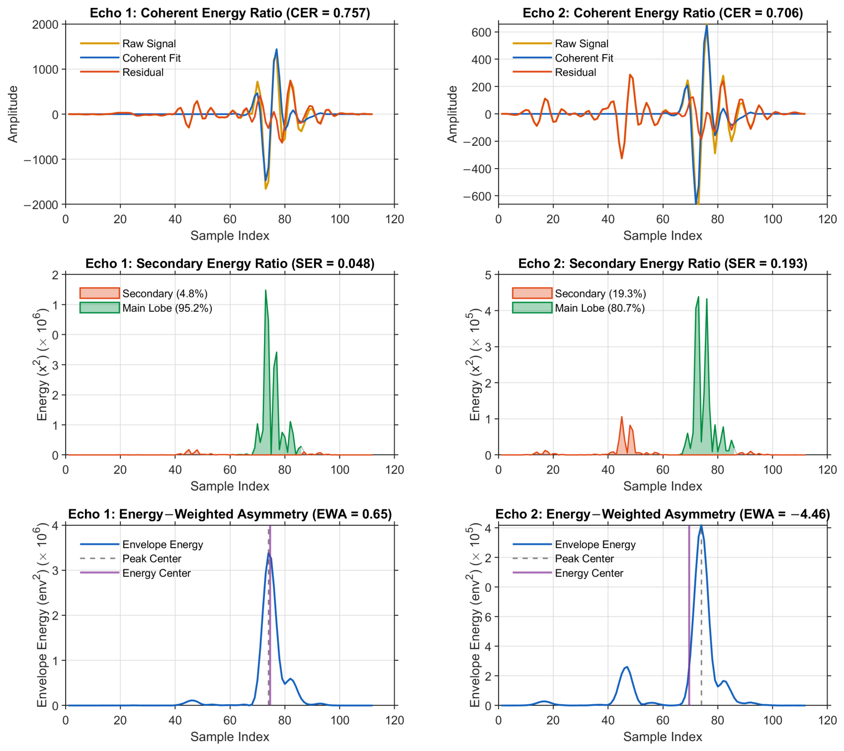
Appendix C. Geometric Derivation of Cross-Path Propagation Delays
This appendix presents the ray-tracing derivation for the individual cross-path propagation delays and introduced in Section 2.2.3. After rebounding from the rearside (transducer-coupling) interface, waves participating in cross-path propagation travel obliquely at an angle relative to the transducer normal over an axial distance to illuminate the adjacent reflector. The round-trip excess delay relative to normal incidence for a generic path i is:
where represents the direct axial time-of-flight. The propagation angle is governed by the effective lateral distance a required to span the pit’s lateral extent over axial depth , such that . Applying the small-angle approximation , the excess delay simplifies to:
Evaluating this expression for the two distinct geometric paths gives:
- Backwall cross-path (): The wave spans the pit’s lateral extent over the full sample thickness:
- Pit-wall cross-path (): The wave spans the same lateral extent over the reduced material thickness to the pit-wall:
With respect to axial geometry, depends primarily on overall sample thickness and decreases as the sample becomes thicker (independent of pit depth to this order of approximation). Conversely, increases as the pit becomes deeper at a fixed sample thickness. The two delays therefore diverge from one another as the pit-depth-to-thickness ratio grows.
References
- Bhandari, J.; Khan, F.; Abbassi, R.; Garaniya, V.; Ojeda, R. Modelling of pitting corrosion in marine and offshore steel structures—A technical review. J. Loss Prev. Process Ind. 2015, 37, 39–62. [Google Scholar] [CrossRef] [Scilit]
- Parangusan, H.; Bhadra, J.; Al-Thani, N. A review of passivity breakdown on metal surfaces: Influence of chloride- and sulfide-ion concentrations, temperature, and pH. Emergent Mater. 2021, 4, 1187–1203. [Google Scholar] [CrossRef] [Scilit]
- Kolawole, S.; Kolawole, F.; Enegela, O.; Adewoye, O.; Soboyejo, A.; Soboyejo, W. Pitting Corrosion of a Low Carbon Steel in Corrosive Environments: Experiments and Models. Adv. Mater. Res. 2015, 1132, 349–365. [Google Scholar] [CrossRef] [Scilit]
- Shojai, S.; Schaumann, P.; Brömer, T. Probabilistic modelling of pitting corrosion and its impact on stress concentrations in steel structures in the offshore wind energy. Mar. Struct. 2022, 84, 103232. [Google Scholar] [CrossRef] [Scilit]
- Sofiani, F.M.; Chaudhuri, S.; Elahi, S.; Hectors, K.; De Waele, W. A numerical study on tensile stress concentration in semi-ellipsoidal corrosion pits. Procedia Struct. Integr. 2023, 51, 51–56. [Google Scholar] [CrossRef] [Scilit]
- Okenyi, V.; Bodaghi, M.; Mansfield, N.; Afazov, S.; Siegkas, P. A review of challenges and framework development for corrosion fatigue life assessment of monopile-supported horizontal-axis offshore wind turbines. Ships Offshore Struct. 2024, 19, 1–15. [Google Scholar] [CrossRef] [Scilit]
- Caines, S.; Khan, F.; Shirokoff, J. Analysis of pitting corrosion on steel under insulation in marine environments. J. Loss Prev. Process Ind. 2013, 26, 1466–1483. [Google Scholar] [CrossRef] [Scilit]
- Li, R.; Wang, H.; Zhu, Y.; Mu, X.; Wang, X. Machine learning–assisted in situ corrosion monitoring: A review. Corros. Rev. 2026, 44, 20250014. [Google Scholar] [CrossRef] [Scilit]
- Lamas, J.S.; Tacq, J.; Teerlinck, B. Assessing the potential of electrochemical techniques for monitoring pitting corrosion in carbon steel for offshore structures. Electrochim. Acta 2026, 563, 148721. [Google Scholar] [CrossRef] [Scilit]
- Suzuki, T.; Otaka, N.; Shibano, K.; Fujimoto, Y.; Hagiwara, T. Detection of Pitting Corrosion in Stainless-Steel Sheet Pile Walls Using Deep Learning. Corros. Mater. Degrad. 2026, 7, 23. [Google Scholar] [CrossRef] [Scilit]
- Sriramadasu, R.C.; Banerjee, S.; Lu, Y. Detection and assessment of pitting corrosion in rebars using scattering of ultrasonic guided waves. NDT E Int. 2019, 101, 53–61. [Google Scholar] [CrossRef] [Scilit]
- Sun, X.; Zhang, M.; Gao, W.; Guo, C.; Kong, Q. A novel method for steel bar all-stage pitting corrosion monitoring using the feature-level fusion of ultrasonic direct waves and coda waves. Struct. Health Monit. 2023, 22, 714–729. [Google Scholar] [CrossRef] [Scilit]
- Cao, W.; Wang, K.; Zhou, P.; Yang, X.; Xu, L.; Liu, M.; Fromme, P.; Pang, B.; Chi, R.; Su, Z. Nonlinear ultrasonic evaluation of disorderedly clustered pitting damage using an in situ sensor network. Struct. Health Monit. 2020, 19, 1989–2006. [Google Scholar] [CrossRef] [Scilit]
- Yang, X.; Xue, B.; Jia, L.; Zhang, H. Quantitative analysis of pit defects in an automobile engine cylinder cavity using the radial basis function neural network–genetic algorithm model. Struct. Health Monit. 2017, 16, 696–710. [Google Scholar] [CrossRef] [Scilit]
- Villaverde, E.L.; Croxford, A.J.; Velichko, A. Optimal Extraction of Ultrasonic Scattering Features in Coarse Grained Materials. IEEE Trans. Ultrason. Ferroelectr. Freq. Control 2021, 68, 2238–2250. [Google Scholar] [CrossRef] [Scilit] [PubMed]
- Civera, M.; Surace, C. Non-Destructive Techniques for the Condition and Structural Health Monitoring of Wind Turbines: A Literature Review of the Last 20 Years. Sensors 2022, 22, 1627. [Google Scholar] [CrossRef] [Scilit] [PubMed]
- Wu, Y.; Wang, Y.; Li, D.; Zhang, J. Two-step detection of concrete internal condition using array ultrasound and deep learning. NDT E Int. 2023, 139, 102945. [Google Scholar] [CrossRef] [Scilit]
- Jarvis, A.J.C.; Cegla, F.B.; Bazaz, H.; Lozev, M. Ultrasonic monitoring of pitting corrosion. In Proceedings of the AIP Conference Proceedings, Denver, CO, USA, 15–20 July 2012; Volume 1511, pp. 1312–1319. [Google Scholar] [CrossRef] [Scilit]
- Rodríguez, C.; Biezma, M.V. Detección de la corrosión por picadura en aceros inoxidables empleando ultrasonidos. Rev. Metal. 2014, 50, e005. [Google Scholar] [CrossRef] [Scilit]
- Wangensteen, M.; Franke Johansen, T.; Fatemi, A.; Viggen, E.M.; Eidissen Haugan, L. Pitting detection and characterization from ultrasound timelapse images using convolutional neural networks. IEEE Open J. Instrum. Meas. 2024, 3, 2500212. [Google Scholar] [CrossRef] [Scilit]
- Ha, J.M.; Seung, H.M.; Choi, W. Autoencoder-based detection of near-surface defects in ultrasonic testing. Ultrasonics 2022, 119, 106637. [Google Scholar] [CrossRef] [Scilit] [PubMed]
- Eason, T.J.; Bond, L.J.; Lozev, M.G. Ultrasonic scattering from a hemispherical pit theory and experimental measurement precision. In Proceedings of the AIP Conference Proceedings, Atlanta, GA, USA, 17–22 July 2016; AIP Publishing: Melville, NY, USA, 2017; Volume 1806, p. 050011. [Google Scholar] [CrossRef] [Scilit]
- Xu, W.; Li, X.; Zhang, J.; Xue, Z.; Cao, J. Ultrasonic signal enhancement for coarse grain materials by machine learning analysis. Ultrasonics 2021, 117, 106550. [Google Scholar] [CrossRef] [Scilit] [PubMed]
- Hu, T.; Zhao, J.; Zheng, R.; Wang, P.; Li, X.; Zhang, Q. Ultrasonic based concrete defects identification via wavelet packet transform and GA-BP neural network. PeerJ Comput. Sci. 2021, 7, e635. [Google Scholar] [CrossRef] [Scilit] [PubMed]
- Zhang, B.; Luo, Z.; Hong, X.; Jin, G. Deep learning-based corrosion-like defect localization technique for high-voltage cable aluminum sheaths using guided waves. Meas. Sci. Technol. 2023, 34, 084006. [Google Scholar] [CrossRef] [Scilit]
- Huang, S.; Li, W.; Liao, J. Research on the Multi-Sensor Fusion Model for Pipeline Corrosion and the Identification Method of Pitting Corrosion. Sensors 2026, 26, 936. [Google Scholar] [CrossRef] [Scilit] [PubMed]
- Uhlig, S.; Alkhasli, I.; Schubert, F.; Tschöpe, C.; Wolff, M. A review of synthetic and augmented training data for machine learning in ultrasonic non-destructive evaluation. Ultrasonics 2023, 134, 107041. [Google Scholar] [CrossRef] [Scilit]
- Pyle, R.J.; Bevan, R.L.T.; Hughes, R.R.; Ait Si Ali, A.; Wilcox, P.D. Domain Adapted Deep-Learning for Improved Ultrasonic Crack Characterization Using Limited Experimental Data. IEEE Trans. Ultrason. Ferroelectr. Freq. Control 2022, 69, 1485–1494. [Google Scholar] [CrossRef] [Scilit] [PubMed]
- Thibbotuwa, U.C.; Cortés, A.; Irizar, A. Ultrasound-Based Smart Corrosion Monitoring System for Offshore Wind Turbines. Appl. Sci. 2022, 12, 808. [Google Scholar] [CrossRef] [Scilit]
- Thibbotuwa, U.C.; Cortés, A.; Irizar, A. Small Ultrasound-Based Corrosion Sensor for Intraday Corrosion Rate Estimation. Sensors 2022, 22, 8451. [Google Scholar] [CrossRef] [Scilit] [PubMed]
- Treeby, B.E.; Cox, B.T. k-Wave: MATLAB toolbox for the simulation and reconstruction of photoacoustic wave fields. J. Biomed. Opt. 2010, 15, 021314. [Google Scholar] [CrossRef] [Scilit] [PubMed]
- TECNALIA. Harshlab: Floating Offshore Laboratory for Materials Testing. Available online: https://harshlab.eu/ (accessed on 1 July 2026).
- Treeby, B.E.; Jaros, J.; Rohrbach, D.; Cox, B.T. Modelling elastic wave propagation using the k-Wave MATLAB Toolbox. In IEEE International Ultrasonics Symposium; IEEE: New York, NY, USA, 2014; pp. 146–149. [Google Scholar] [CrossRef] [Scilit]
- Perez-Diego, M.; Thibbotuwa, U.C.; Cortés, A.; Irizar, A. Coating Thickness Estimation Using a CNN-Enhanced Ultrasound Echo-Based Deconvolution. Sensors 2025, 25, 6234. [Google Scholar] [CrossRef] [Scilit] [PubMed]
- Ben-David, S.; Blitzer, J.; Crammer, K.; Pereira, F. Analysis of Representations for Domain Adaptation. In Proceedings of the Advances in Neural Information Processing Systems; Schölkopf, B., Platt, J., Hofmann, T., Eds.; MIT Press: Cambridge, MA, USA, 2006; Volume 19, pp. 137–144. [Google Scholar]
- Ganin, Y.; Ustinova, E.; Ajakan, H.; Germain, P.; Larochelle, H.; Laviolette, F.; Marchand, M.; Lempitsky, V. Domain-Adversarial Training of Neural Networks. J. Mach. Learn. Res. 2016, 17, 1–35. Available online: http://jmlr.org/papers/v17/15-239.html (accessed on 13 July 2026).
- Mehri Sofiani, F.; Chaudhuri, S.; Elahi, S.; Hectors, K.; De Waele, W. Quantitative analysis of the correlation between geometric parameters of pits and stress concentration factors for a plate subject to uniaxial tensile stress. Theor. Appl. Fract. Mech. 2023, 127, 104081. [Google Scholar] [CrossRef] [Scilit]
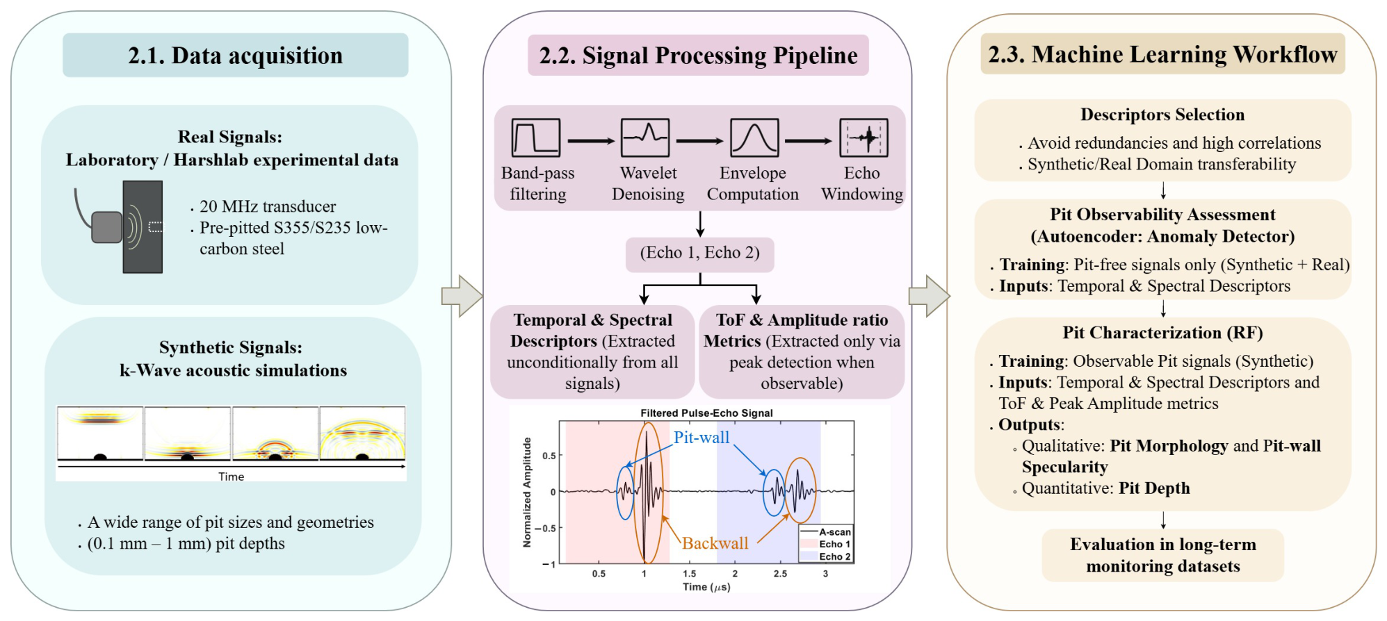
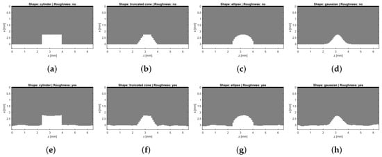
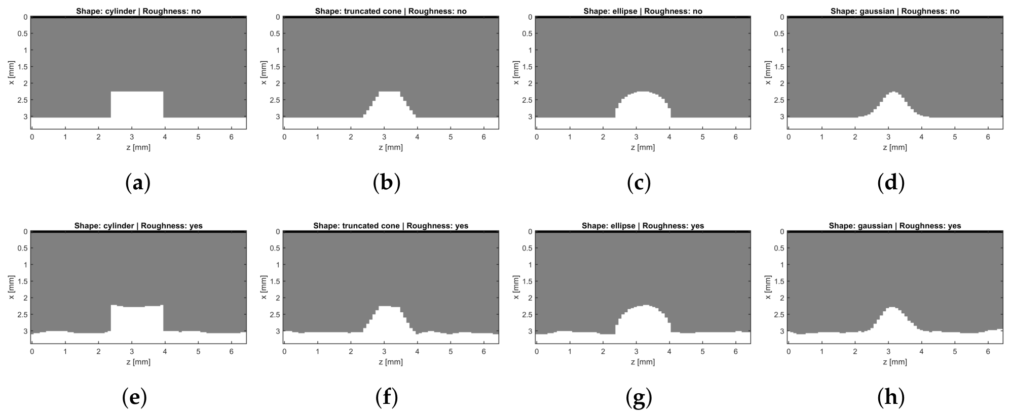
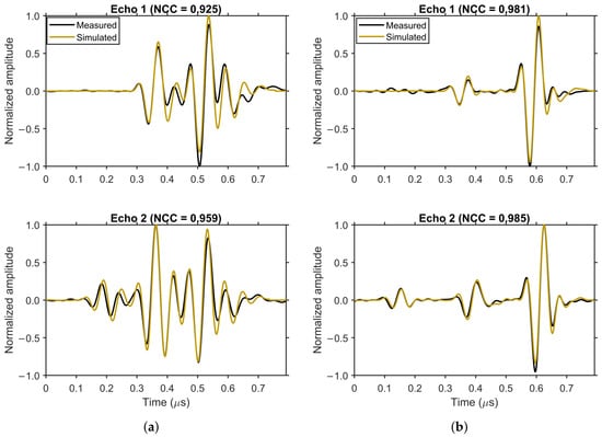
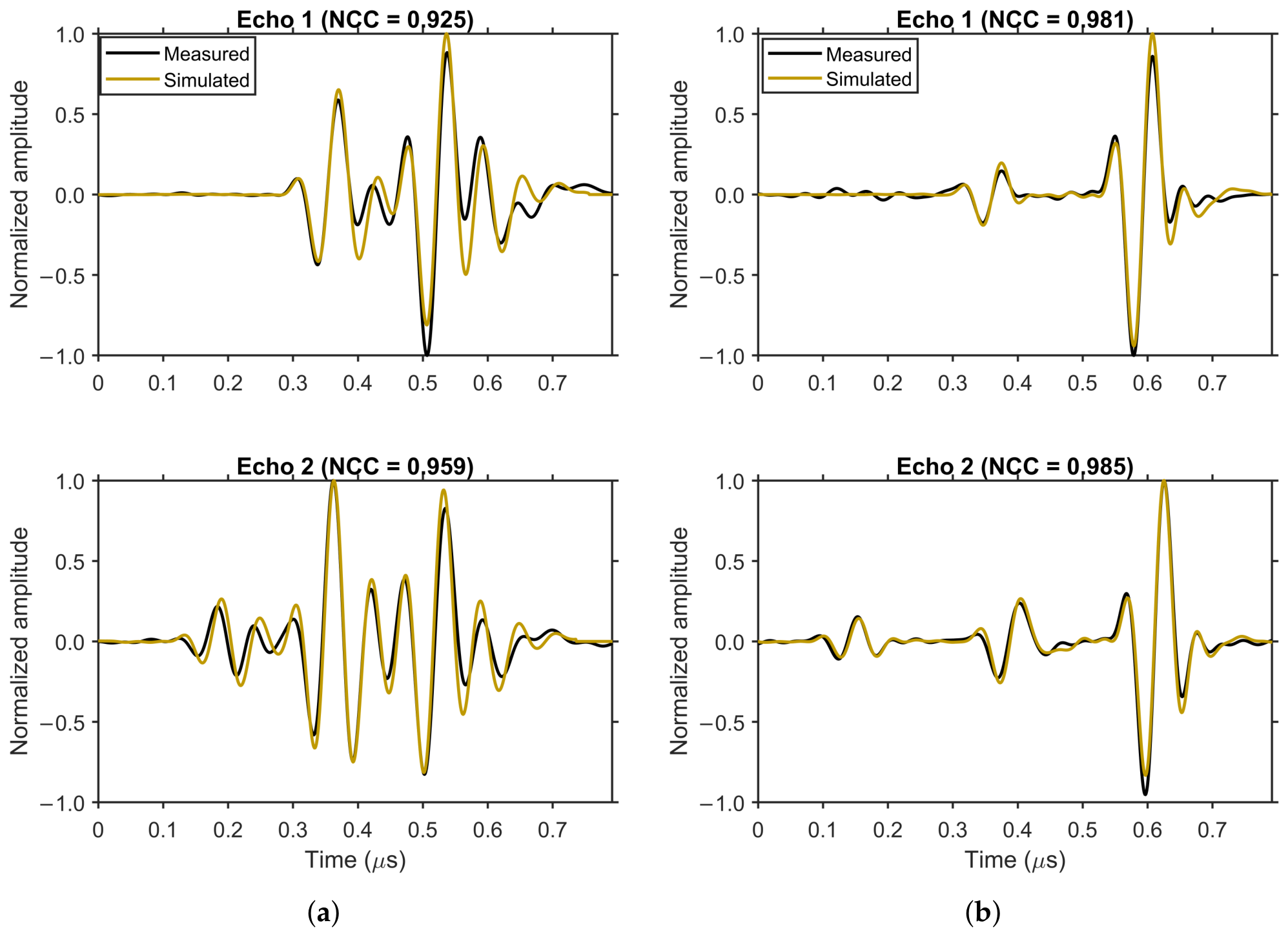
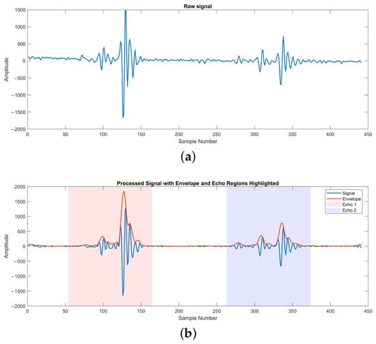
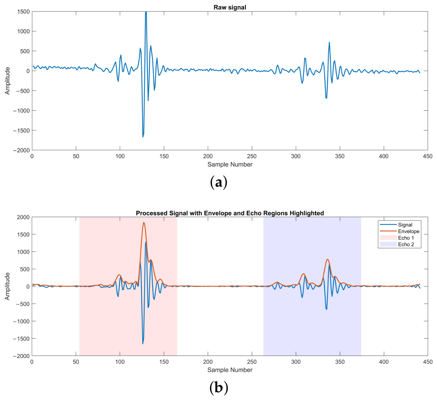
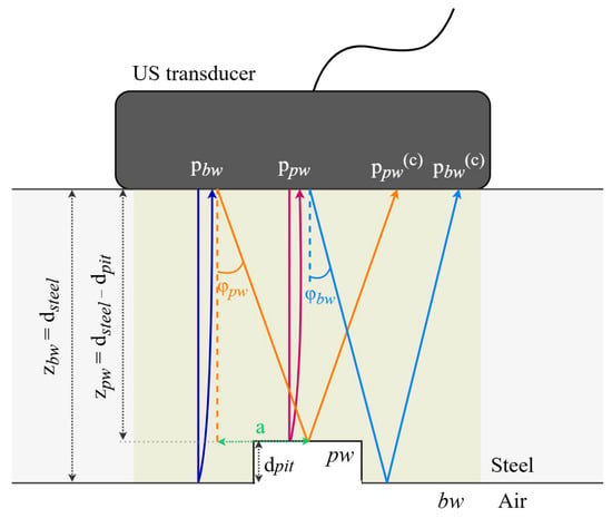
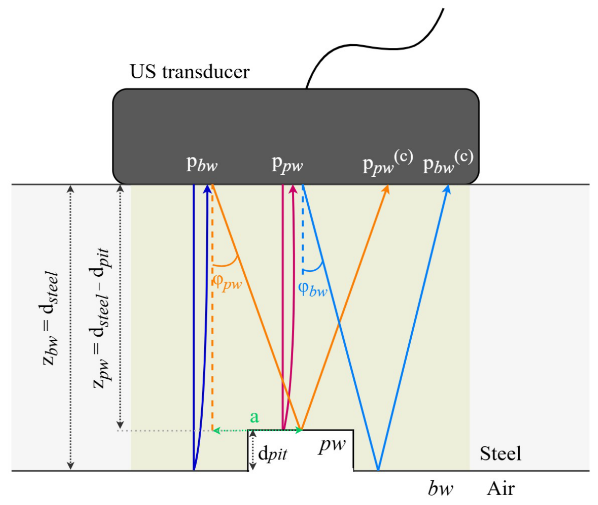
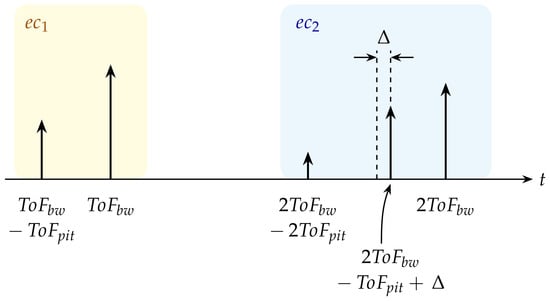
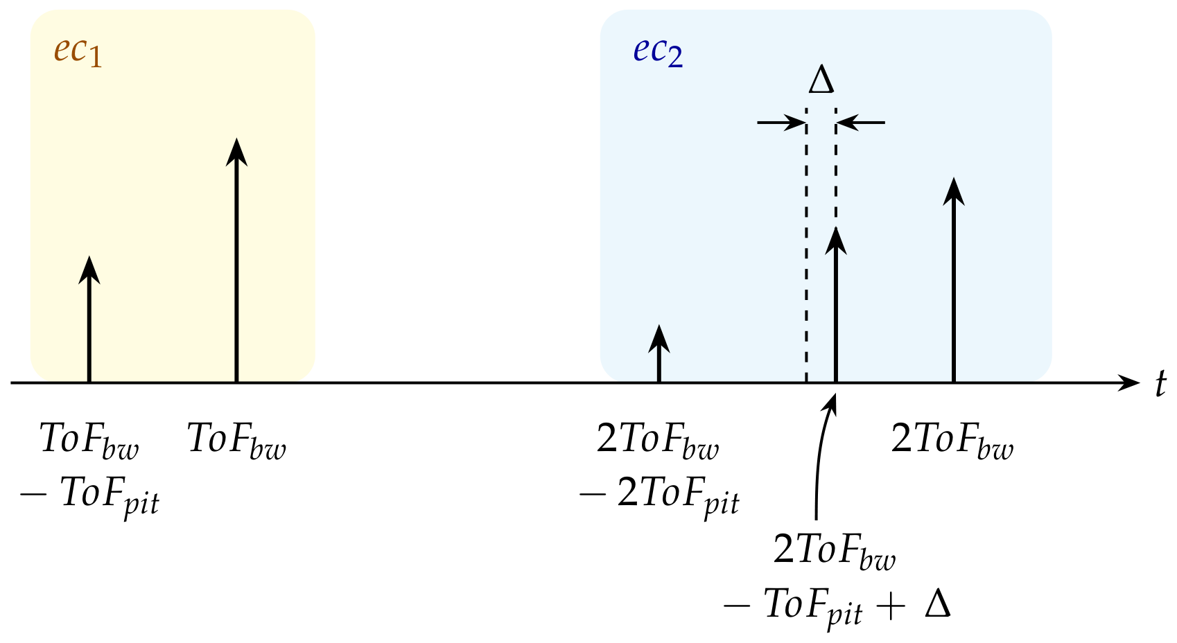
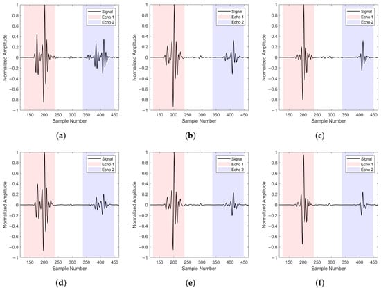
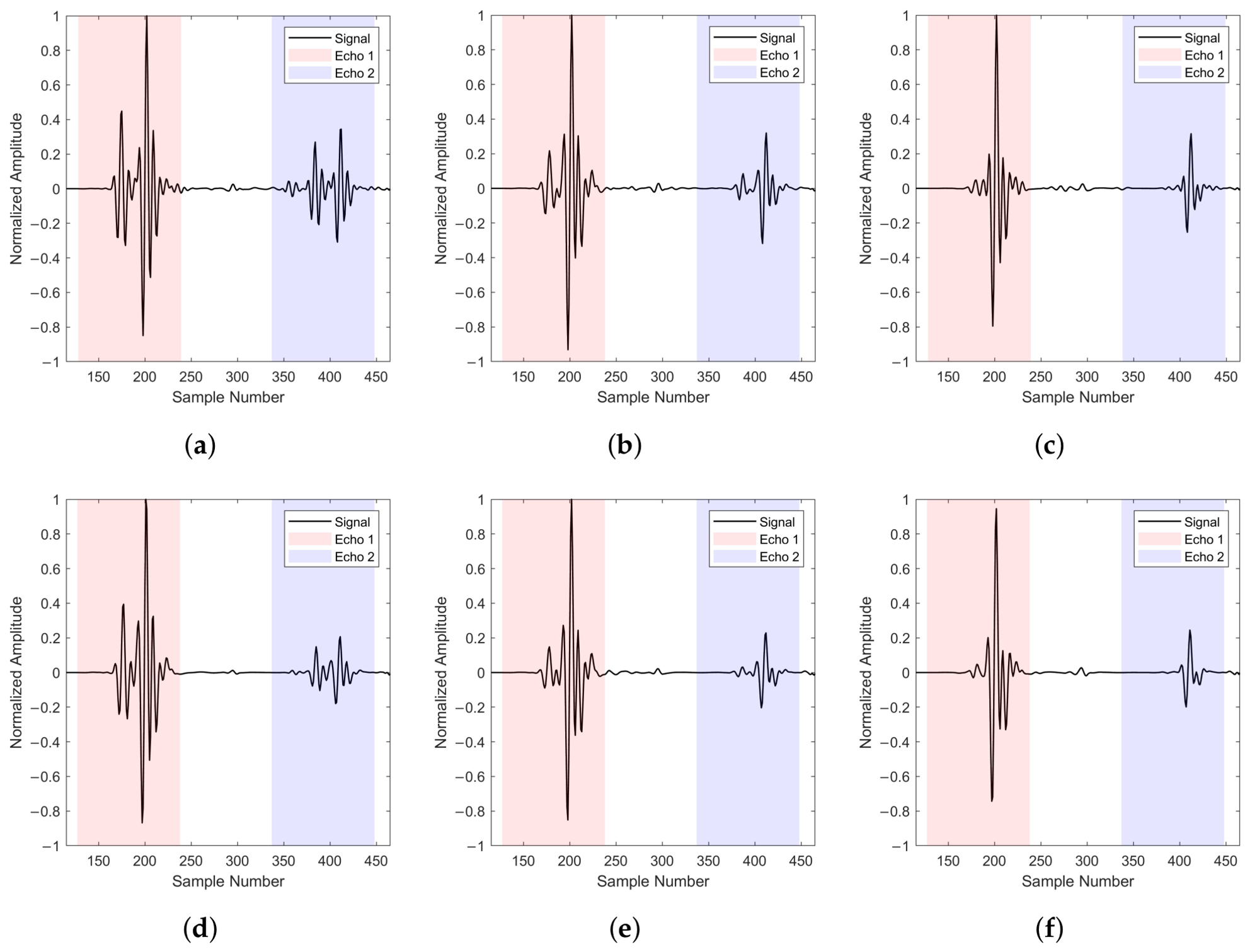
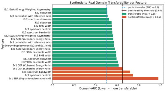
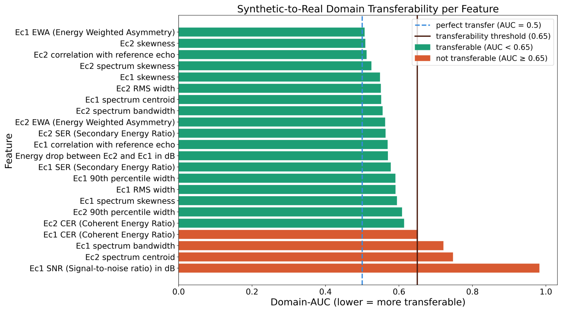
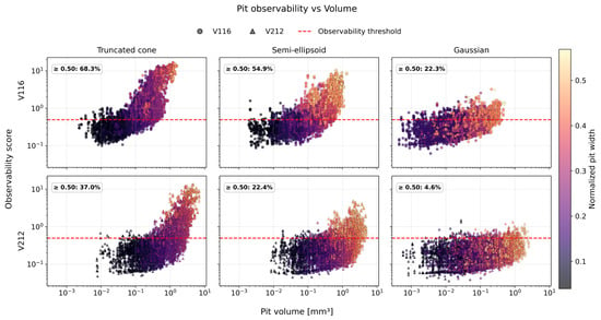
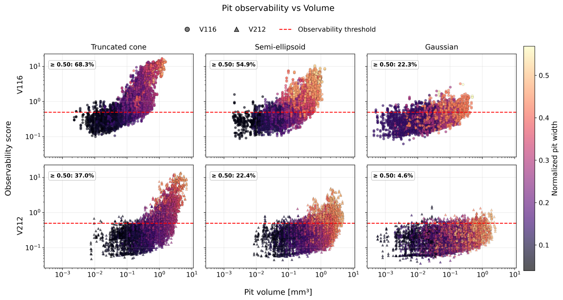
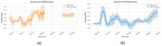
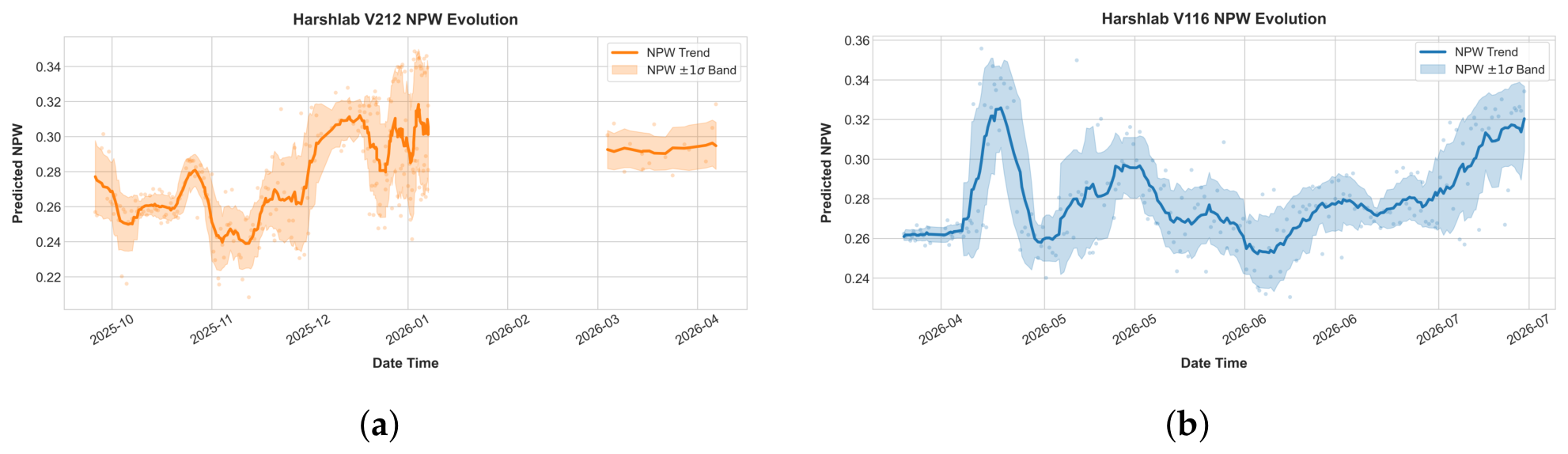
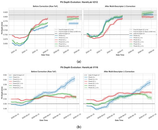
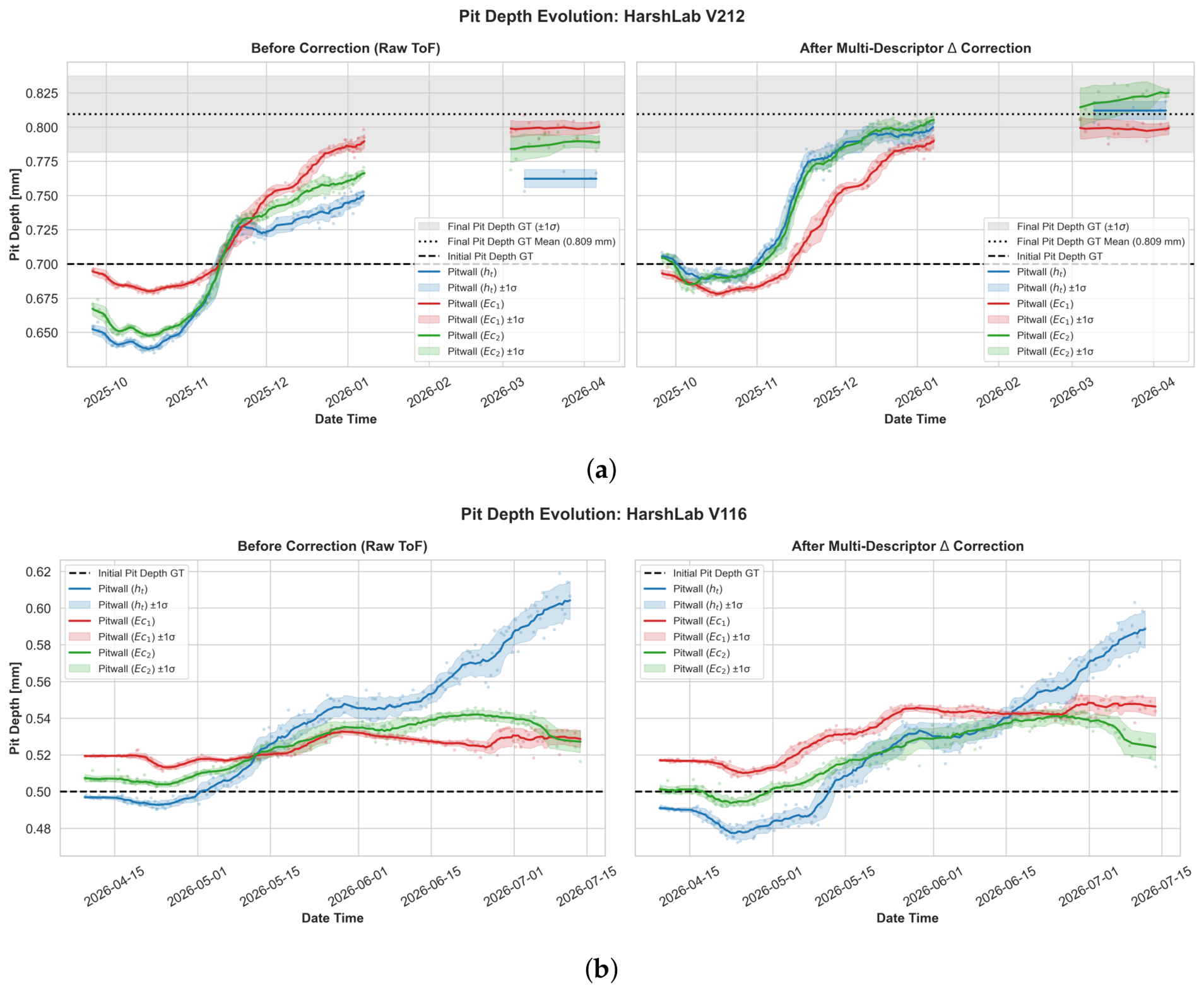
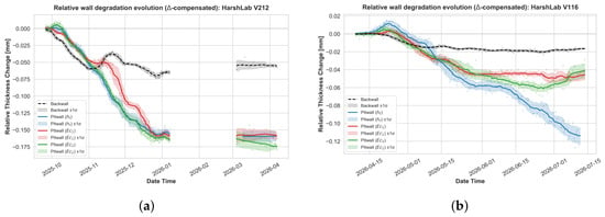
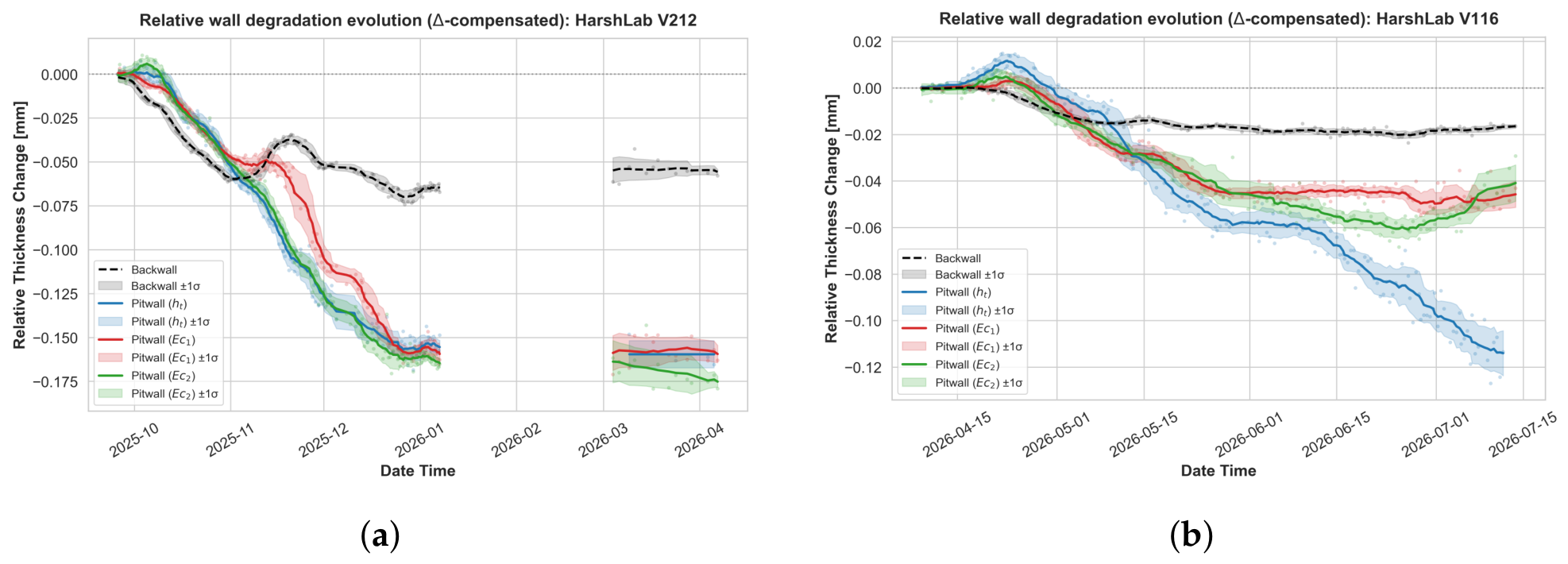
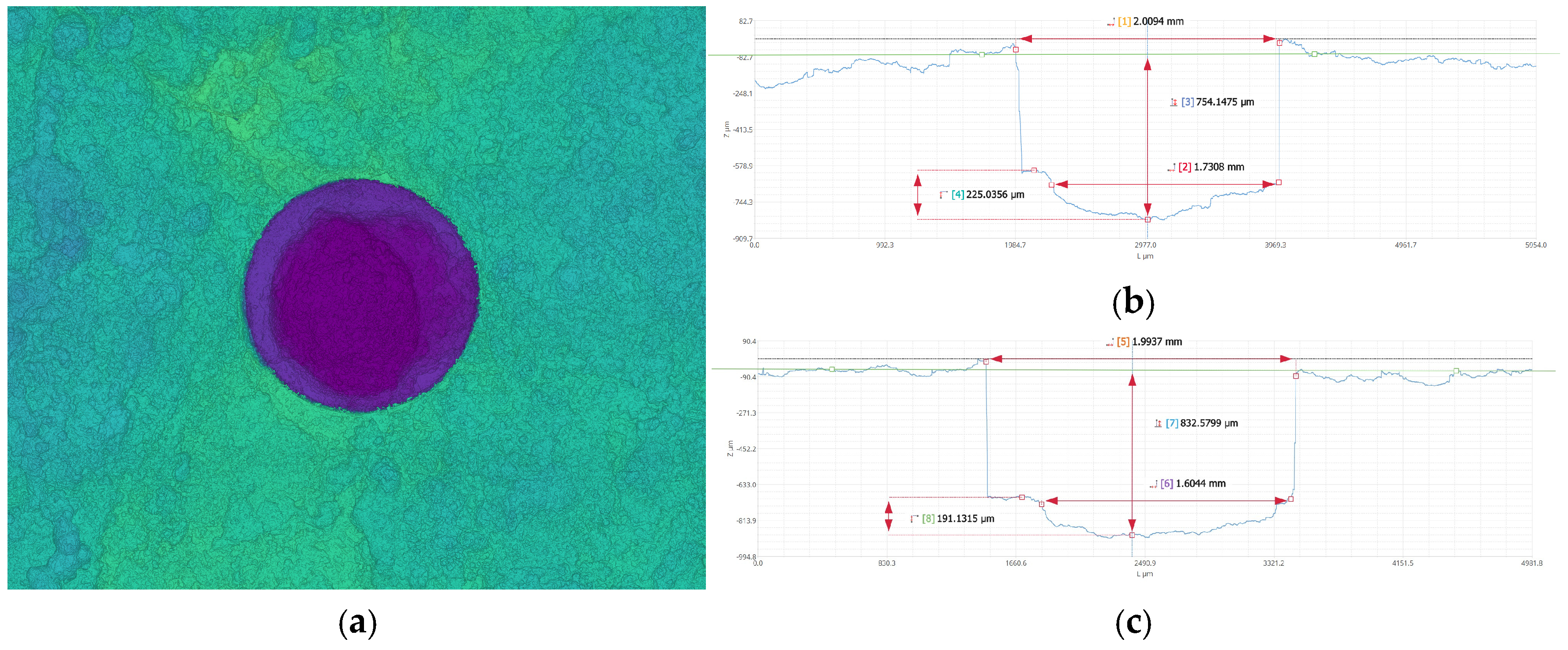

Disclaimer/Publisher’s Note: The statements, opinions and data contained in all publications are solely those of the individual author(s) and contributor(s) and not of MDPI and/or the editor(s). MDPI and/or the editor(s) disclaim responsibility for any injury to people or property resulting from any ideas, methods, instructions or products referred to in the content. |
© 2026 by the authors. Licensee MDPI, Basel, Switzerland. This article is an open access article distributed under the terms and conditions of the Creative Commons Attribution (CC BY) license.