Unified EEG Feature Extraction for Cross-Subject Driver State Recognition and a Leakage-Free Safe-Stop Trigger Mechanism

Abstract

Electroencephalography (EEG)-based Brain–Computer Interfaces offer direct insight into a driver’s mental state, relevant to autonomous-vehicle perception stacks. This work addresses vigilance/drowsiness specifically, one of several driver states relevant to Level 3 takeover readiness. Detecting drowsiness before handover in Level 3 vehicles requires balancing high-dimensional EEG features against the real-time demands of a lightweight safe-stop trigger mechanism. We present a complete pipeline: a standardized 22-feature-per-channel schema extracted across four driving-related EEG datasets, an autoencoder achieving over 95% dimensionality reduction with minimal performance loss, and a classifier driving a constant-deceleration kinematic profile used to obtain a measurable latency figure, evaluated under a fully subject-disjoint, leakage-free protocol. Leave-one-subject-out cross-validation on the vigilance dataset yields a mean macro-F1 of 0.793 ± 0.163 (0.763 ± 0.155 on an alternative run, within expected autoencoder-retraining variance). Extending compression evaluation to all four datasets shows preserved or improved performance on three, with a small cost on the fourth. The full decision chain completes in under 1 ms (mean 0.13 ms) on standard hardware; this covers the perception-to-trigger budget only, excluding solver latency that an optimization-based planner (MPC/CBF-QP) would add downstream. These findings show cognitive-state-aware safe-stop triggering is implementation-viable, while highlighting the calibration and cross-machine validation needed for deployment.

1. Introduction

Brain–Computer Interfaces (BCIs) based on electroencephalography (EEG) have been explored across a wide range of domains, from clinical rehabilitation and assistive communication to gaming and workload monitoring in high-stakes professions such as aviation [1]. Among these applications, driver monitoring has emerged as a particularly promising use case: EEG offers a direct, continuous signal of a driver’s cognitive and emotional state, making it a candidate for improving safety through advanced driver assistance systems [2,3]. In this paper, we use “driver state” specifically to mean vigilance/drowsiness, the construct that our four datasets and downstream classifier target; we do not claim coverage of the broader space of driver states (e.g., distraction from secondary tasks) that a complete Level 3 readiness assessment would ultimately require. Drowsiness detection in particular has shown promise for reducing accident risk, since a large share of road accidents are attributed to reduced driver vigilance rather than external hazards.

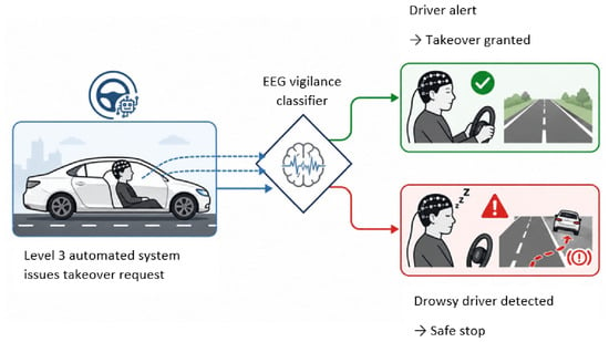
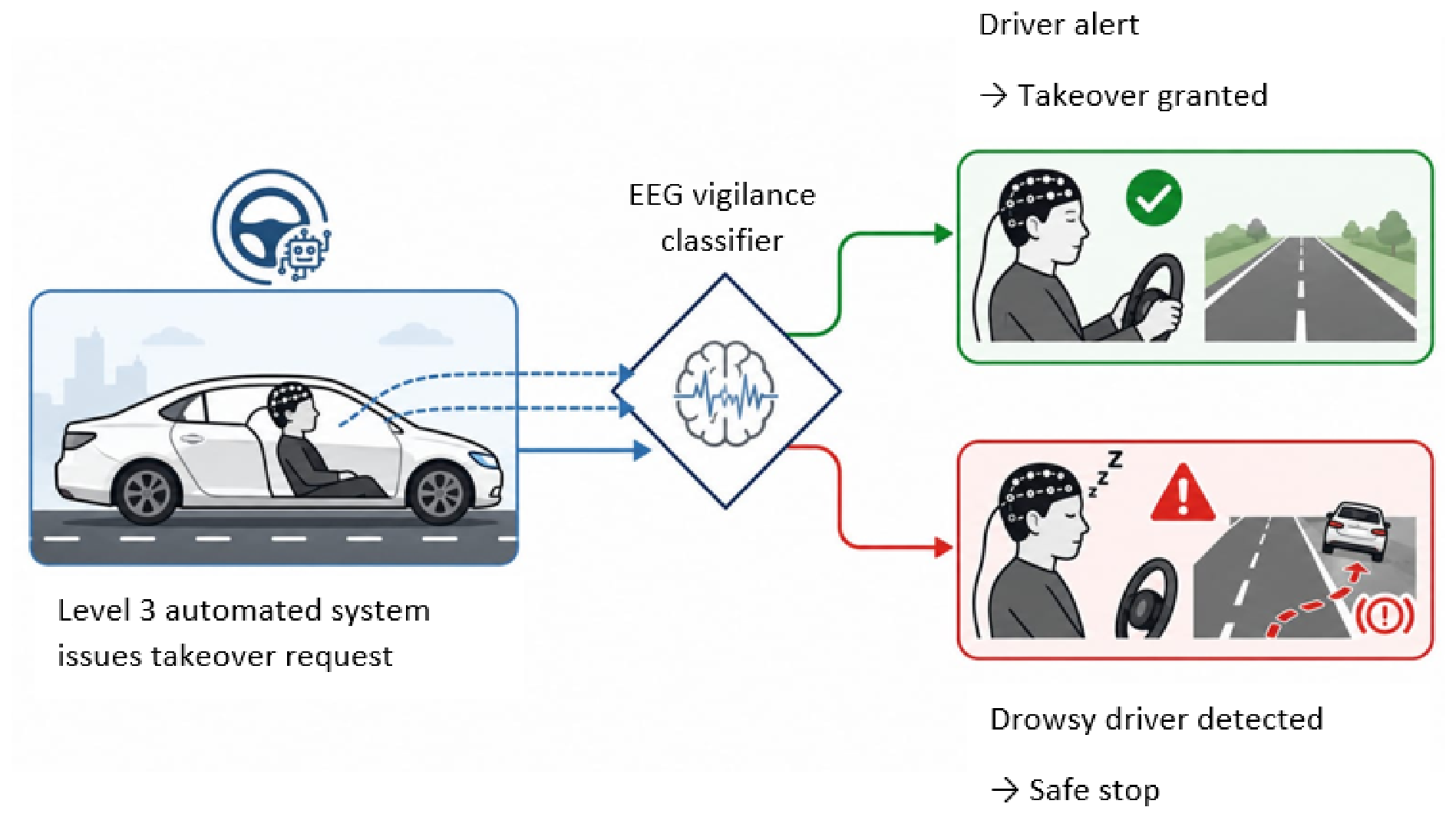
The need for reliable vigilance assessment takes on particular concreteness when considering SAE Level 3 (Conditional Automation) cars, where the automation system is capable of driving by itself under certain conditions, yet can at any time ask for the driver to take control. This is in contrast with Level 2, where the driver needs to keep an eye out at all times, or Level 4, where the car is supposed to reach a stable state without any human interference. This creates a recurring, safety-critical decision point: before granting control back to the driver, the vehicle must assess whether that driver is cognitively fit to drive [4]. Figure 1 illustrates this handover scenario and the two possible outcomes depending on the driver’s vigilance state. We emphasize that Figure 1 and the pipeline that follows address vigilance-based readiness specifically; a deployed L3 system would need this vigilance assessment as one input among several (e.g., gaze/attention, task-engagement and behavioral monitoring) rather than as a sufficient condition on its own.

Figure 1. Level 3 handover decision scenario.

For autonomous navigation and safe-stop triggering, vigilance monitoring serves as a perception layer. Prior to a vehicle-to-driver control transfer, the autonomous system needs to establish the ability of the human operator to take control [5]. Development in this area faces several challenges. First, publicly available EEG data for driving tasks vary significantly in terms of number of channels, recording device used and the semantic meaning of the labels, making it impossible to combine them [6]. Second, high-dimensional EEG feature vectors create computational barriers inconsistent with the requirements of real-time performance on embedded automotive hardware [7]. This work designs an end-to-end pipeline that covers heterogeneous sensor harmonization, latent-space reduction, cross-subject evaluation of classifiers and safe-stop trigger computation.

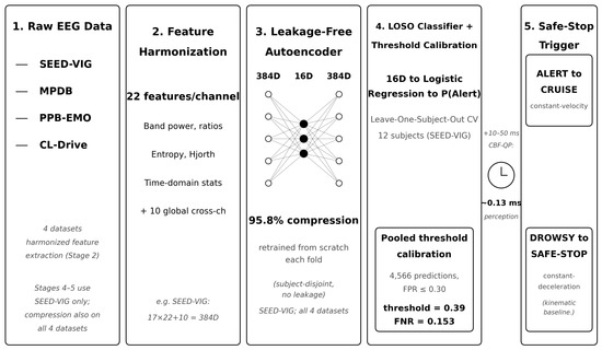
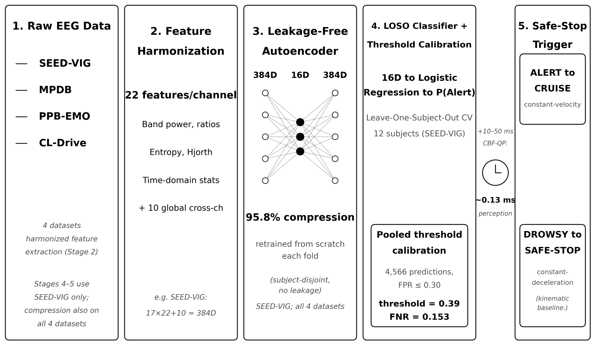
The central, rigorously evaluated contribution of this work is cross-subject vigilance classification from a compressed, hardware-harmonized EEG representation. The kinematic safe-stop trigger (Section 3.4) is a secondary, illustrative output, included to obtain a concrete, measurable latency figure for the perception pipeline (Section 4.6). It uses a standard feature extraction process for four distinct datasets for driving-related activities through electroencephalography (EEG). Out of these datasets, this paper focuses its cross-subject LOSO evaluation on the dataset with the strongest baseline signal, vigilance (SEED-VIG), while also extending the compression evaluation itself to all four datasets (Section 4.2) using matched, leakage-free folds, providing partial cross-hardware evidence rather than relying on SEED-VIG alone. As far as we know, this is one of the first works in the literature of EEG-driven autonomous vehicles to include all of the following, which are usually treated independently: (i) a completely subject-disjoint and leakage-free evaluation of both the compression phase and the subsequent classification, carried out through subject-based Leave-One-Subject-Out LOSO experiments on all the subjects; (ii) the direct integration of the compressed signal into a latency-benchmarking safe-stop trigger and not only the performance evaluation of classification methods; and (iii) the actual wall-clock time of the perception-and-classification stage on a stated hardware platform. While previous works usually focused only on one of compression [8], cross-subject generalization [9], or driver-state-aware control of the vehicle [10], we cover all three aspects together with their own limitations. The complete pipeline is illustrated in Figure 2.

Figure 2. Complete EEG-to-safe-stop trigger pipeline.

The rest of the paper is organized in the following way: Section 2 gives an overview of the related literature in the context of EEG-based feature extraction, driver state recognition, and safe-stop triggering and handover planning. Section 3 describes the methodology used in this research, which includes dataset description, feature extraction, a leakage-free autoencoder, vigilance-driven safe-stop triggering, and validation methods. Section 4 covers the experimental results, which include the baseline, leave-one-subject-out cross-validation, safety measures and latency tests. Section 5 will consider practical applications and limitations of the research.

2. Related Works

2.1. EEG-Based Feature Extraction and Signal Processing

EEG has been validated as a reliable indicator of cognitive load and vigilance in driving scenarios [11,12]. Foundational studies established that spectral power in the theta (4–8 Hz) and alpha (8–13 Hz) bands, particularly over frontal and occipital regions, correlates strongly with drowsiness onset [1,13]. However, these early studies were primarily conducted under controlled laboratory conditions using within-subject evaluation protocols. They did not address the computational latency required for real-time deployment in a vehicle, nor did they evaluate performance on unseen subjects without recalibration, two critical requirements for an autonomous driving system that must work for any driver immediately upon entry.

To deploy complex machine learning models on resource-constrained edge devices, dimensionality reduction techniques such as autoencoders have gained traction [7]. Autoencoders learn non-linear manifolds that preserve discriminative structure while drastically reducing input size [14]. ROS-Neuro, for example, reported greater than 90% dimensionality reduction with sub-millisecond streaming jitter for online BCI applications [8]. More recent work has explored variational autoencoders for stochastic latent representations [15] and knowledge distillation from large teacher models to compact student networks [16]. However, most BCI compression studies evaluate reconstruction error or within-subject classification, omitting wall-clock latency measurements on actual hardware and leakage-free cross-subject evaluation [17]. For autonomous vehicle applications specifically, inference latency must be significantly faster than the vehicle’s mechanical response time (typically 10–100 ms) to be practical [18]. We build on this line of work by evaluating both compression fidelity and end-to-end latency in a subject-disjoint protocol.

2.2. Driver State Recognition and Cross-Subject Generalization

Deep learning approaches have been applied to EEG-based drowsiness detection, including convolutional neural networks (CNNs) operating on raw or spectrally transformed signals [19,20], hybrid CNN-LSTM architectures for temporal modeling [21], and transformer-based models that capture long-range dependencies in EEG sequences [22]. Despite achieving high within-dataset accuracy, these models are computationally expensive, with parameter counts in the millions, making them unsuitable for resource-constrained automotive edge hardware. Furthermore, most deep learning studies continue to evaluate performance on within-subject splits, leaving cross-subject generalization unaddressed [23]. Notable exceptions include the work of Zheng and Lu [24], who proposed a multimodal vigilance estimation framework using EEG and forehead EOG; however, even that work did not evaluate computational latency for embedded deployment.

Inter-subject variability has been established as a major impediment to deploying BCI systems across new users without recalibration [9,25]. Variability arises from anatomical differences (skull thickness, cortical folding), psychological state, and electrode placement errors, all of which degrade cross-subject transfer performance [26]. A dedicated review of intra- and inter-subject variability in EEG-based sensorimotor BCI catalogs these sources and argues that within-subject evaluation protocols systematically overstate real-world deployment performance [9]. To mitigate this, several data alignment and domain adaptation techniques have been proposed, including Euclidean Alignment (EA) [27], Correlation Alignment (CORAL) [28] and Riemannian Procrustes Analysis [29]. Comparative evaluations under Leave-One-Subject-Out cross-validation show that EA consistently improves cross-subject transfer relative to no alignment. However, these alignment methods are typically applied at the covariance or feature level; applying them directly to a compressed latent space, as we do here, remains an open question.

A related open question is how correctness and quality can be assured when a pipeline is built entirely on public datasets whose collection protocols the present authors do not control. We address this in two ways in this study: (i) Table 1’s dataset specifications were cross-checked directly against each dataset’s original publication rather than transcribed from secondary sources. (ii) Every classification result reported here uses subject-disjoint, leakage-free evaluation specifically because public datasets’ documentation of collection conditions is often incomplete, making leakage-based inflation of performance a particular risk when reusing third-party data as-is.

2.3. Safe-Stop Triggering and Handover Planning

In autonomous path planning, transitioning from autonomous to manual control requires confidence in the driver’s cognitive capacity [5]. A frequently overlooked constraint is decision latency: the time between sensing driver state and adjusting the trajectory. High latency delays braking and increases stopping distance [30]. Prior work on emergency and safe-stop trajectory planning has generally treated the triggering condition (e.g., sensor failure, detected obstacle) as instantaneous or externally given, focusing instead on trajectory optimization [30,31,32]. More recent work has integrated physiological signals as soft constraints in Model Predictive Control (MPC) frameworks [33,34], though these integrations typically assume the physiological signal is available with zero latency, which is rarely true in practice.

Bridging consumer-grade biosensors with autonomous driving safety more broadly requires quantifying perception uncertainty and embedding it into contingency-aware planning; a recent example of this paradigm is the interaction-aware motion planning framework of Tian et al. [35], which explicitly quantifies perception uncertainty for safe ramp-driving maneuvers. Our contribution is complementary to and narrower than this line of work: rather than proposing a new trajectory optimizer or uncertainty-aware planner, we measure the latency cost of the upstream perception decision, the EEG-to-classification step, that would need to feed into such a planner, using a constant-deceleration profile so that the reported latency reflects the perception pipeline rather than trajectory-optimizer complexity. We return to this connection in Section 5, where we discuss how the continuous (rather than binarized) output of our classifier could serve as exactly the kind of perception-uncertainty signal such frameworks require.

To our knowledge, no prior work combines all three of the following elements in a single pipeline: (i) fully subject-disjoint, leakage-free evaluation of both the compression stage and the downstream classifier using Leave-One-Subject-Out cross-validation across all available subjects; (ii) integration of the compressed representation into a latency-instrumented safe-stop trigger; and (iii) explicit reporting of the limitations of each component (underpowered compression test, per-subject variance, and cross-hardware transfer as future work) rather than presenting only favorable results. This paper addresses these gaps by constructing a complete EEG-to-trigger pipeline evaluated under conditions that reflect the challenges of real-world deployment: unseen drivers, resource-constrained computation, and a measured latency budget.

3. Methods

The proposed pipeline is structured into three sequentially executed stages, bridging raw physiological acquisition to a physical safe-stop trigger: (i) sensor harmonization and standardized feature extraction, (ii) non-linear dimensionality reduction via a leakage-free autoencoder, and (iii) real-time classification and kinematic trigger computation.

The following subsections detail each component, emphasizing the design choices made to satisfy the competing objectives of classification fidelity, cross-subject generalization and sub-millisecond inference latency.

3.1. Datasets

To rigorously evaluate the framework’s adaptability to different sensor setups, we utilized four publicly available driving-related EEG datasets, summarized in Table 1. These datasets span the hardware spectrum encountered in automotive BCI, from high-density clinical caps to low-channel consumer wearables, and cover driving behavior, emotion, cognitive load, and vigilance. Table 1 details each dataset’s target construct, demographics (N, age, gender), EEG channel count, and acquisition hardware. Configurations range from 59-channel clinical systems (MPDB, NeuSen W, 1000 Hz) and 18-channel systems (SEED-VIG, Neuroscan, 1000 Hz) to a 32-channel research-grade system (PPB-EMO, EnobioNE, 500 Hz) and a 4-channel consumer headband (CL-Drive, Muse S, 256 Hz). Sample sizes range from 21 to 40 subjects, with mean ages from 23.3 to 28.1 years.

Table 1. Summary of the four datasets: construct, demographics, and acquisition hardware.

Dataset	Construct	N	Age	Gender	EEG ch.	Hardware
MPDB [36]	Driving behaviour	35 a	20–60 (mean 25.1)	26 M, 9 F	59	NeuSen W64 (Neuracle Technology Co., Ltd., Changzhou, China), 1000 Hz
PPB-EMO [37]	Emotion	40	19–58 (mean 28.1)	31 M, 9 F	32	ENOBIO 20 (Neuroelectrics, Barcelona, Spain), 500 Hz
SEED-VIG [24]	Vigilance	23 b	23.3 ± 1.4	11 M, 12 F	18 c	Neuroscan SynAmps2 (Compumedics Neuroscan, Charlotte, NC, USA), 200 Hz
CL-Drive [38]	Cognitive load	21	26.9 (mean)	6 M, 15 F	4	Muse S (InteraXon Inc., Toronto, ON, Canada), 256 Hz

^a The released MPDB dataset contains 35 subjects; this study used a 30-subject subset. ^b The released SEED-VIG dataset contains 23 subjects; this study used a 12-subject subset. ^c The released SEED-VIG dataset provides 18 EEG channels; this study excluded one channel prior to feature extraction, yielding the 17 channels used in the 384-dimensional schema (17 × 22 + 10).

Table 1. Summary of the four datasets: construct, demographics, and acquisition hardware.

Dataset	Construct	N	Age	Gender	EEG ch.	Hardware
MPDB [36]	Driving behaviour	35 a	20–60 (mean 25.1)	26 M, 9 F	59	NeuSen W64 (Neuracle Technology Co., Ltd., Changzhou, China), 1000 Hz
PPB-EMO [37]	Emotion	40	19–58 (mean 28.1)	31 M, 9 F	32	ENOBIO 20 (Neuroelectrics, Barcelona, Spain), 500 Hz
SEED-VIG [24]	Vigilance	23 b	23.3 ± 1.4	11 M, 12 F	18 c	Neuroscan SynAmps2 (Compumedics Neuroscan, Charlotte, NC, USA), 200 Hz
CL-Drive [38]	Cognitive load	21	26.9 (mean)	6 M, 15 F	4	Muse S (InteraXon Inc., Toronto, ON, Canada), 256 Hz

^a The released MPDB dataset contains 35 subjects; this study used a 30-subject subset. ^b The released SEED-VIG dataset contains 23 subjects; this study used a 12-subject subset. ^c The released SEED-VIG dataset provides 18 EEG channels; this study excluded one channel prior to feature extraction, yielding the 17 channels used in the 384-dimensional schema (17 × 22 + 10).

Channel count varies substantially across these datasets (4 to 59) and this has a direct, measurable effect on the results reported in this study: our extended compression analysis shows that the two highest-channel-count datasets (MPDB, PPB-EMO) have the weakest matched-fold baselines (macro-F1 0.499 and 0.474, respectively), while the lower-dimensional SEED-VIG (17 channels, 384D) achieves the strongest (0.834). We do not interpret this as channel count alone driving generalizability; native sampling rate, electrode placement density, and label granularity all differ jointly across datasets and are confounded with channel count in this comparison. A second confound visible in Table 1 is demographic: the released datasets jointly skew male (62.2%), the direction of bias reverses across datasets, and all mean ages fall within 23.3–28.1 years, leaving older drivers unrepresented. Neither confound can be isolated in a four-dataset comparison, so both are reported as scope limitations rather than findings. Age and gender figures describe the released datasets; see the table footnotes for the subsets and channel configurations used here.

Among these four datasets, SEED-VIG exhibited the highest baseline physiological signal-to-noise ratio (as quantified by the within-dataset macro-F1 of 0.838 in Table 2), making it the most suitable candidate for the rigorous cross-subject compression and LOSO study. The remaining datasets (MPDB, PPB-EMO, CL-Drive) serve to validate the generality of the feature-extraction stage; we additionally extend the compression evaluation itself to all four datasets using matched, leakage-free folds, and report the results plainly rather than generalizing a SEED-VIG-only finding. The feature-extraction stage is applied identically and successfully across all four hardware platforms (Table 1), while the benefit of the compression stage specifically is dataset-dependent rather than uniformly demonstrated. True zero-shot transfer of a single autoencoder trained on one dataset to another dataset’s raw feature space remains to be assessed in future work (Section 5).

Table 2. Within-dataset baseline performance (subject-grouped 5-fold CV, native features).

Dataset	Channels	Accuracy	Macro-F1
MPDB	59	0.704 ± 0.026	0.449
PPB-EMO	32	0.486 ± 0.055	0.434
SEED-VIG	17	0.841 ± 0.072	0.838
CL-Drive	4	0.620 ± 0.033	0.612

3.2. Hardware-Agnostic Preprocessing Pipeline

To transform heterogeneous raw signals into a uniform format without losing neurophysiological interpretability, a standardized pipeline was applied. Recordings were segmented using 2.0 s sliding windows with a hop size of 0.5 s (75% overlap). A 2.0 s window was chosen to balance temporal resolution with the stationarity required for reliable spectral analysis, while the high overlap ensures no transient drowsiness events are split across window boundaries.

For each valid window, a fixed schema of 22 identical features was computed per channel:

• Relative band powers (5): Power Spectral Density (PSD) was estimated using Welch’s method. Power was integrated over five canonical frequency bands (delta, theta, alpha, beta, gamma), with each band normalized by the total power (1–45 Hz) to yield dimensionless relative band powers.
• Inter-band ratios (3): Theta/Alpha, Alpha/Beta, and Theta/Beta ratios, which are established neurophysiological correlates of cognitive workload and vigilance fluctuations.
• Entropy (2): Spectral entropy and permutation entropy, both normalized to the [0, 1] range to measure signal complexity.
• Hjorth parameters (3): Activity (variance), Mobility, and Complexity in the time domain.
• Time-domain statistics (9): Mean, variance, standard deviation, skewness, kurtosis, RMS, peak-to-peak amplitude, zero-crossing rate and signal slope (linear trend, via least-squares fit over the window).

Finally, 10 global cross-channel statistics (mean and variance of the 5 relative band powers across all available channels) were appended to capture spatial distribution without requiring channel alignment.

A critical hardware-level intervention was amplitude calibration: consumer-grade headsets (PPB-EMO, CL-Drive) output raw data in integer hardware counts (∼${10}^6$ to ${10}^8$) rather than physiological microvolts. A global multiplicative scaling factor of ${10}^{-6}$ was applied prior to feature extraction to restore physiologically plausible ranges. For the 17-channel SEED-VIG dataset, this schema yielded a standardized 384-dimensional vector per window ($[17\times 22]+10=384$).

3.3. Leakage-Free Autoencoder Architecture

Latent space compression was performed using a fully connected autoencoder. The architecture was intentionally kept shallow to minimize inference latency for the downstream trigger module:

• Encoder: Input ($D=384$) → Dense (128 units, ReLU) → Bottleneck ($L=16$).
• Decoder: Bottleneck (16) → Dense (128 units, ReLU) → Output ($D=384$).

The model was optimized using the Adam optimizer (learning rate $=1\times {10}^{-3}$) with Mean Squared Error (MSE) loss. MSE was chosen over perceptual losses to strictly preserve the absolute magnitudes of spectral features, which are critical for the downstream logistic regression classifier. The bottleneck dimension of 16 was chosen empirically as the inflection point in our compression curve, representing a Pareto-optimal trade-off where reduction to 8D degraded downstream macro-F1 (0.836 vs. 0.844), and expansion to 32D yielded no meaningful accuracy gain.

Leakage prevention protocol: A common flaw in the BCI literature is training an autoencoder on the entire dataset prior to cross-validation, which leaks test-set structural information into the training phase and artificially inflates compression performance. To prevent this, for every cross-validation fold (compression evaluation) and every LOSO fold (classification evaluation), the autoencoder was retrained from scratch using only the training subjects from that specific fold. The final optimized encoder size was 203 KB, easily satisfying the memory constraints of automotive-grade embedded systems.

3.4. Vigilance-Triggered Safe-Stop Mechanism

To evaluate real-time feasibility, the 16D latent vector was classified using a regularized Logistic Regression (LR) model. LR was chosen over deep networks for the trigger module because it provides a continuous probability output (useful for future Model Predictive Control integration) while adding near-zero inference latency.

The kinematic profile below specifies a constant-deceleration braking law, included to provide a concrete, measurable latency figure for the upstream perception pipeline (Section 4.6). We refer to this component as a safe-stop trigger mechanism throughout, reflecting its role as the interface between classification and actuation. If the LR model classified the driver as drowsy, a kinematic safe-stop trajectory was computed to serve as a concrete physical output for the latency benchmark. We modeled a minimum safe-stop maneuver assuming constant comfortable deceleration ($a=2.0$ m/s²). This rate represents a gentle-to-moderate braking profile typical of commercial adaptive cruise control and collision mitigation systems [30], balancing collision avoidance with passenger comfort. The kinematic equations governing the trajectory are:

$$d={\displaystyle \frac{v_0^2}{2a}},v\left(t\right)=v_0-at$$

(1)

where $v_0$ is the initial vehicle speed and d is the stopping distance. If the driver is classified as alert, a constant-velocity cruise trajectory is maintained.

3.5. Evaluation Protocol

3.5.1. Within-Dataset Baselines

A Random Forest classifier (300 trees, max_depth = 10, class_weight = ‘balanced’) was evaluated per dataset using subject-grouped 5-fold cross-validation on the native, uncompressed feature sets. Random Forest was selected as a stable baseline due to its inherent robustness to multi-collinearity in high-dimensional spectral features and minimal hyperparameter sensitivity, which isolates the effect of the compression stage itself. GroupKFold (scikit-learn 1.3.0, https://scikit-learn.org, accessed on 15 September 2026) ensures that all windows from a single subject are kept in the same fold, preventing subject-specific signal leakage from artificially inflating baseline accuracy.

3.5.2. Compression Evaluation (Paired Design)

To rigorously test if compression degrades performance, a single subject-grouped 5-fold split was used. Crucially, both the raw 384D and compressed 16D representations were evaluated on the identical held-out subjects per fold. This paired design ensures that any performance difference is strictly due to the autoencoder’s information loss, not differences in which subjects happened to be held out. A Wilcoxon signed-rank test was applied to the 5 paired macro-F1 scores.

3.5.3. Extended Compression Evaluation Across All Four Datasets

To directly address whether compression generalizes beyond SEED-VIG, we repeated the paired evaluation on MPDB, PPB-EMO, and CL-Drive using the same autoencoder architecture and the same matched-fold protocol. For SEED-VIG (12 subjects), true Leave-One-Subject-Out was used. For MPDB (30 subjects), PPB-EMO (40 subjects), and CL-Drive (21 subjects), a subject-grouped 10-fold protocol was used in place of exhaustive LOSO purely for computational tractability (retraining an autoencoder per fold scales with subject count); we report this protocol difference explicitly rather than presenting all four datasets as evaluated identically. PPB-EMO’s native label (a nominal 7-class emotion identifier) was converted to a binary target using a valence-based grouping (negative-valence emotions vs. positive/neutral) rather than an arbitrary ordinal split, since the emotion identifier carries no inherent order.

3.5.4. Leave-One-Subject-Out (LOSO) Cross-Validation

To evaluate cross-subject generalization on the compressed space, we employed a strict LOSO protocol on SEED-VIG. For each of the 12 folds, the following points are true:

• The autoencoder was retrained unsupervised on the 11 non-held-out subjects.
• A Logistic Regression classifier was trained on those 11 subjects’ encoded 16D features and labels.
• To prevent overfitting given the small sample size (11 subjects), regularization strength (C) was selected via internal subject-grouped 3-fold cross-validation within the 11 training subjects, sweeping $C\in \{0.001,0.01,0.1,1.0,10.0\}$.
• The held-out subject was encoded with the frozen autoencoder and classified once with the frozen LR model.

3.5.5. Pooled Threshold Sensitivity Analysis

To address whether the classifier’s decision threshold, not just its discriminative power, can reduce missed-drowsiness events, we pooled the held-out predicted probabilities from all 12 LOSO folds above (4566 windows total) and swept the decision threshold from 0.01 to 0.99, computing FPR and FNR at each point. We report the full sweep alongside a single recommended operating point, selected as the threshold minimizing FNR subject to FPR ≤ 0.30—a safety-motivated constraint reflecting that a missed drowsy driver (false negative) is a more severe failure mode than a conservative, unnecessary caution response (false positive) in this application. We additionally report per-subject optimal thresholds to characterize how much an adaptive, condition-specific threshold could further reduce FNR relative to a single pooled operating point; these per-subject values are a diagnostic upper bound computed on held-out data and are not proposed as a deployable per-subject calibration method without further nested validation.

4. Results

We present the experimental outcomes of the core evaluations designed to validate the proposed pipeline: (i) within-dataset baselines establishing feature extraction performance across heterogeneous hardware; (ii) paired compression experiments quantifying the accuracy-cost of 95.8% dimensionality reduction on SEED-VIG, extended to all four datasets; (iii) Leave-One-Subject-Out cross-validation assessing cross-subject generalization on the compressed 16D latent space; and (iv) a pooled threshold sensitivity analysis addressing the operating-point trade-off between missed-drowsiness and false-alarm rates. Each subsection concludes with a contextual interpretation of the findings in relation to the practical constraints of autonomous vehicle deployment.

4.1. Within-Domain Baselines

Table 2 reports within-dataset classification performance. SEED-VIG yields the strongest signal (macro-F1 0.838). This is expected: vigilance is heavily correlated with global shifts in alpha and theta band power, which are captured by the 10 global cross-channel features. PPB-EMO (0.434) and MPDB (0.449) yielded lower scores, reflecting the inherent difficulty of decoding high-level constructs (nominal emotions, complex motor behaviors) using high-dimensional consumer and clinical hardware and global spectral summaries. CL-Drive (0.612) showed moderate performance, suggesting that a 4-channel Muse S can capture gross cognitive load shifts. These baselines motivated selecting SEED-VIG for the latency-critical compression deep dive.

4.2. Latent Space Compression

Table 3 shows the results of the strictly paired 5-fold experiments on SEED-VIG. Compressing the 384D vector to 16D (a 95.8% reduction) resulted in a mean macro-F1 reduction of only 0.025 (0.838 to 0.813). A Wilcoxon signed-rank test on the five paired folds could not find a statistically significant difference between the two conditions ($p=0.125$). This result is consistent with prior studies on EEG autoencoder compression, which report that well-structured spectral features can be projected into low-dimensional manifolds (8–32 dimensions) with minimal downstream classification degradation [8,14]. Our contribution extends this finding by demonstrating that such compression remains effective under a leakage-free, subject-disjoint protocol, where the autoencoder is retrained per fold rather than on the entire dataset a priori.

Table 3. Leakage-free autoencoder compression on SEED-VIG (paired subject-grouped 5-fold CV, Random Forest classifier).

Method	Dimensions	Reduction	Macro-F1
Raw features (baseline)	384	0%	0.838 ± 0.074
Autoencoder (16D)	16	95.8%	0.813 ± 0.076

While this test is underpowered due to the small number of paired folds ($n=5$) and should not be taken as definitive proof of absolute equivalence, the raw means and standard deviations confirm that the difference is marginal. The difference favored the uncompressed data in four out of five folds, indicating that the autoencoder discards a small amount of discriminative noise rather than critical signal. For an embedded automotive system, a 2.5% accuracy trade-off for a 95.8% reduction in dimensionality and a model size of just 203 KB represents a highly favorable engineering compromise.

4.3. Extended Compression Evaluation Across All Four Datasets

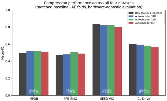
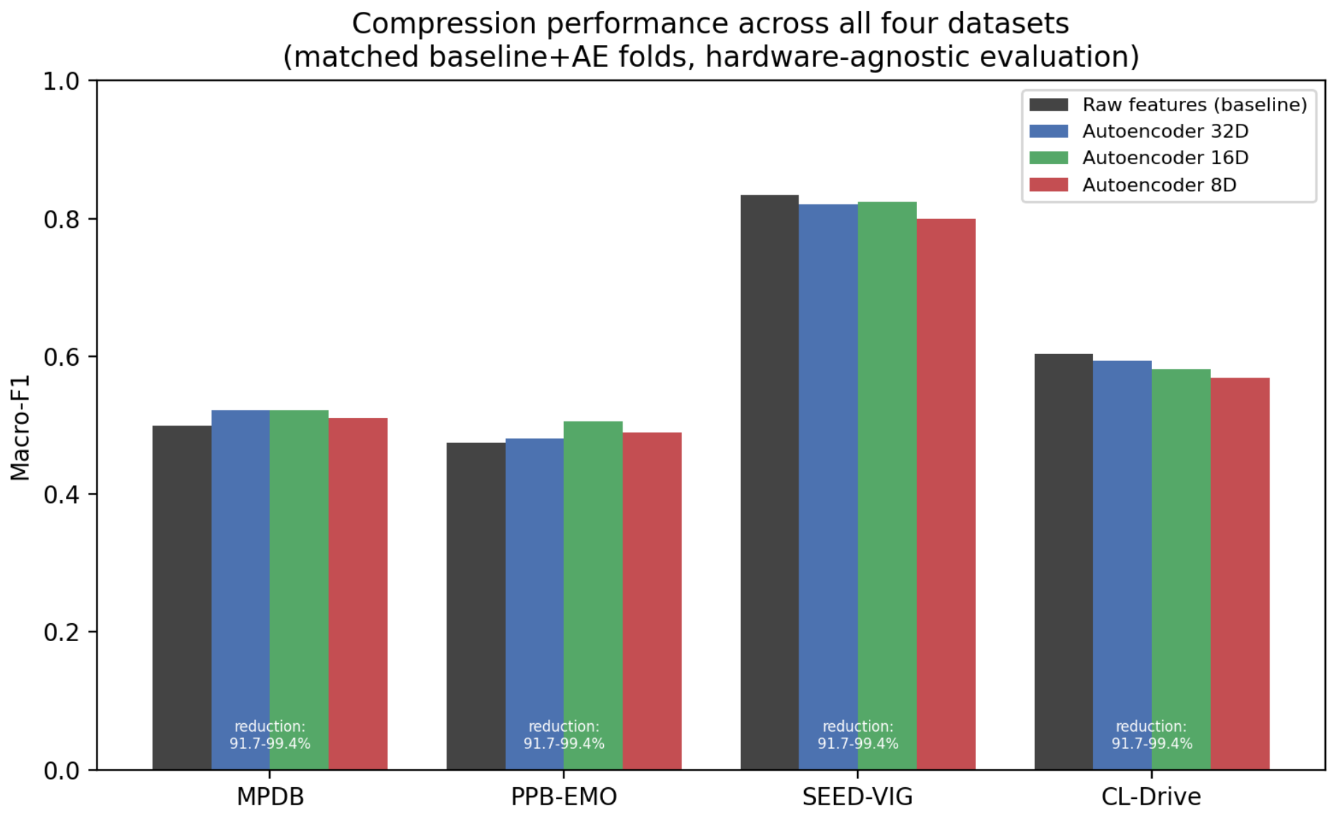
Table 4 and Figure 3 report the matched-fold compression results across all four datasets, directly addressing whether the hardware-agnostic claim extends beyond SEED-VIG. Compression to 16D preserves or improves macro-F1 on three of four datasets: MPDB (0.499 → 0.522, $+0.023$), PPB-EMO (0.474 → 0.506, $+0.031$), and SEED-VIG (0.834 → 0.824, $-0.010$, within one standard deviation of baseline). CL-Drive shows a small consistent cost ($-0.009$ to $-0.034$ depending on latent dimension). We interpret the improvement on MPDB and PPB-EMO—the two highest-native-dimensionality datasets (1308D and 650D, respectively)—as consistent with the autoencoder acting as an implicit denoising/regularization step on noisier, higher-dimensional raw features, rather than as evidence the framework improves signal quality universally. We report this dataset-dependent pattern plainly: compression’s benefit is not uniform across hardware platforms, and CL-Drive in particular does not show a hardware-agnostic compression benefit in this evaluation.

Table 4. Compression performance across all four datasets (matched baseline + autoencoder folds). MPDB/PPB-EMO/CL-Drive use subject-grouped 10-fold CV (true LOSO was computationally impractical given fold-wise autoencoder retraining at these subject counts); SEED-VIG uses true 12-fold LOSO.

Dataset	Raw F1	AE-32D	AE-16D	AE-8D
MPDB	0.499 ± 0.037	0.521 ± 0.025	0.522 ± 0.026	0.511 ± 0.013
PPB-EMO	0.474 ± 0.057	0.481 ± 0.048	0.506 ± 0.030	0.489 ± 0.025
SEED-VIG	0.834 ± 0.119	0.821 ± 0.130	0.824 ± 0.124	0.800 ± 0.142
CL-Drive	0.603 ± 0.044	0.594 ± 0.065	0.581 ± 0.055	0.569 ± 0.048

Figure 3. Compression performance (macro-F1) across all four datasets and three latent dimensions, matched baseline and autoencoder folds.

4.4. Cross-Subject Generalization (LOSO)

Table 5 contains the per-subject LOSO results for logistic regression on the 16D latent space. The mean macro-F1 across all 12 subjects is 0.793 ± 0.163 (range 0.421–0.991). An alternative run of this exact protocol yielded a mean of 0.763 ± 0.155. The two runs differ within the expected range of fold-to-fold stochasticity from retraining the autoencoder from scratch in every fold. To contextualize this result, prior studies employing leave-one-subject-out protocols on SEED-VIG with classical spectral features have reported macro-F1 scores ranging from 0.68 to 0.78 [2,9]. Our 16D compressed representation achieves a mean in this range or above it depending on the run, indicating that the autoencoder preserves discriminative information. Combined with the matched raw-feature baseline reported for every dataset in Table 4, this provides a matched-fold reference under an identical fold structure as the compressed representation.

Table 5. LOSO results for vigilance classification on the 16D latent space (Logistic Regression).

Subject	N (Windows)	FPR	FNR	Macro-F1
1	228	0.000	0.018	0.991
2	166	0.000	0.916	0.421
3	452	0.420	0.071	0.747
4	498	0.012	0.486	0.736
5	194	0.052	0.021	0.964
6	642	0.012	0.358	0.809
7	392	0.041	0.485	0.724
8	142	0.225	0.028	0.872
9	404	0.099	0.114	0.894
10	704	0.014	0.136	0.924
11	420	0.667	0.181	0.550
12	324	0.130	0.105	0.883
Mean ± Std	–	0.139 ± 0.207	0.243 ± 0.271	0.793 ± 0.163

Notably, the internal hyperparameter search consistently selected strong L2 regularization ($C=0.001$) for the majority of folds. This indicates that in a low-sample-size, high-dimensional cross-subject BCI setting, a heavily regularized linear decision boundary generalizes significantly better than a complex one, preventing the model from memorizing the training subjects’ idiosyncratic baseline shifts.

Two subjects (Subjects 2 and 11) yielded substantially lower F1 scores (0.421 and 0.550). Without access to the original raw EEG for quality audit, we attribute this to the well-documented inter-subject variability in EEG-based BCI, which can be driven by differences in skull conductivity, variable electrode impedance, or unique artifact profiles [9,39]. This is corroborated by the pooled threshold analysis below (Section 4.4): Subject 2 also has the highest FNR at the pooled operating threshold (0.578), independently confirming it as a genuinely difficult case rather than a single-metric artifact. Despite these outliers, the majority of subjects (7 out of 12) achieved an F1 $>0.75$, confirming that the 16D manifold retains a robust cross-subject discriminative structure.

4.5. Pooled Threshold Sensitivity Analysis

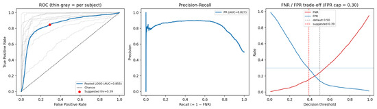
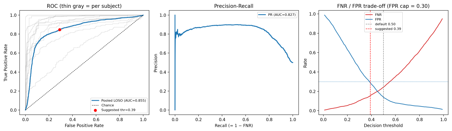
Table 5’s per-subject FPR/FNR values are each computed at a default threshold of 0.50 in isolation per fold. The classifier’s discriminative power alone does not determine the trade-off between missed-drowsiness events and false alarms; this trade-off is set by the decision threshold. We therefore pool all 4566 held-out predictions across the 12 LOSO folds and analyze the full threshold sweep. At the pooled default threshold (0.50): FPR = 0.139, FNR = 0.243. Applying our stated selection criterion (minimize FNR subject to FPR ≤ 0.30) identifies threshold = 0.39, at which FNR falls further to 0.153 (FPR rises to 0.290). Figure 4 shows the full ROC curve, precision–recall curve, and FPR/FNR-vs-threshold trade-off (pooled AUC = 0.855; PR AUC = 0.827).

Figure 4. Pooled LOSO threshold sensitivity analysis (all 12 subjects, 4566 windows). (Left): ROC curve with thin per-subject curves shown for context. (Center): Precision–Recall curve. (Right): FPR/FNR vs. decision threshold, with the FPR ≤ 0.30 constraint and the selected operating point (threshold = 0.39) marked.

Table 6 reports per-subject optimal thresholds under the same FPR ≤ 0.30 constraint, directly addressing the suggestion that the operating point could be varied by condition (e.g., highway vs. urban, or here, by subject as a proxy for individual calibration). Optimal per-subject thresholds range from 0.14 to 0.91 (median 0.31), and for 4 of 12 subjects, a subject-specific threshold reduces FNR by more than 0.05 relative to the single pooled threshold. Subjects 2, 7, and 4—notably, Subject 2 is also the lowest-F1 outlier in Table 5—show the largest pooled-threshold FNR (0.578, 0.439, 0.273, respectively), reinforcing that a single global threshold is a reasonable default but leaves room for per-driver calibration, consistent with the seat/mirror-adjustment analogy raised in our Section 5.

Table 6. Per-subject threshold sensitivity at the pooled operating threshold (0.39) vs. each subject’s own optimal threshold (FPR ≤ 0.30 constraint). Reported for the three subjects with the highest FNR at the pooled threshold.

Subject	N	FNR (Pooled Thr. 0.39)	FPR (Pooled Thr.)	Own Optimal Thr.	FNR (Own Thr.)
2	166	0.578	0.012	0.17	0.084
7	392	0.439	0.082	0.14	0.255
4	498	0.273	0.112	0.33	0.177

4.6. End-to-End Perception-and-Trigger Latency

The wall-time latency of the perception-and-classification pipeline (EEG feature encoding → LR classification → kinematic trigger computation) is given in Table 7. In order to set the software lower bound of an embedded CPU, benchmarks were performed using one core of an Intel Xeon CPU @ 2.20GHz (Intel, Santa Clara, CA, USA) using the default Google Colab runtime (Google LLC, Mountain View, CA, USA; https://colab.research.google.com, accessed on 15 September 2026), which represents a constrained system without GPU computing support.

Table 7. End-to-end perception-and-trigger decision latency, benchmarked on held-out test subjects.

Metric	Latency (ms)
Mean	0.13
Standard Deviation	0.03
P50 (Median)	0.12
P95	0.18
P99	0.22
Maximum	0.25

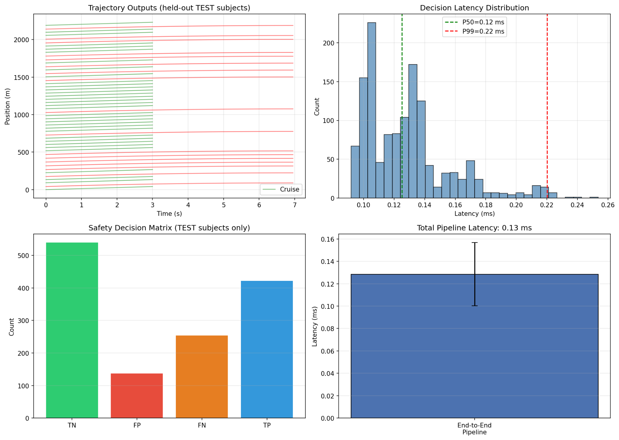
Mean total latency is 0.13 ms, and the maximum worst-case P99 latency is 0.22 ms. We clarify explicitly that this 0.13 ms figure represents the perception-and-classification budget only (feature encoding through kinematic trigger computation) and is not the total latency of a closed-loop vehicle control cycle. Integrating this perception pipeline into a true optimization-based planner (e.g., MPC or CBF-QP) would introduce additional, separately budgeted solver latency, typically in the order of 10–50 ms in real-time automotive implementations, which is not included in Table 7 below.

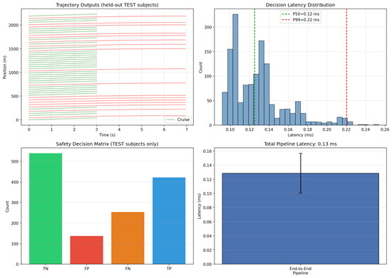
In order to put this into perspective in light of the special Path Planning issue, driving at an average speed of 50 km/h (13.9 m/s), P99 latency will amount to a travel distance of only 0.0031 m (3.1 mm) for the perception stage measured here. The above mentioned latency is lower than the inference times typically reported for deep convolutional neural networks on EEG classification problems and is comparable with the sub-millisecond jitter benchmarks of ROS-Neuro’s compressed streaming pipelines [8]. Figure 5 illustrates representative trigger outcomes and latency distributions on held-out test subjects.

Figure 5. End-to-end perception-to-trigger demonstration on held-out test subjects. (Top-left) Trajectory outputs showing normal cruise (green) versus triggered safe-stops (red). (Top-right) Distribution of total decision latencies across the test set. (Bottom-left) Aggregate safety decision matrix counts (illustrative single-split figures; see Section 4.4 for the primary pooled 12-subject analysis). (Bottom-right) Total pipeline latency benchmark.

5. Discussion

This study’s main conclusion is that a cognitively aware perception-and-trigger pipeline is computationally very simple for the current hardware. However, implementation of these machine learning metrics in an automotive setting involves considering several aspects, including variance reduction between different subjects, safety trade-offs, interfacing with higher level controllers, and the limitations of the current work. As shown in Table 5, the 16D encoding allows for cross-subject detection of vigilance states with an average macro-F1 of 0.793 (0.763 on an alternative run), yet with relatively high variance (0.155–0.163 across runs). For comparison, in previous studies utilizing LOSO validation, the performance of classifiers trained on SEED-VIG with spectral features ranges between 0.68 and 0.78 macro-F1 [2,9]. Our 16D feature is competitive with or exceeds these baselines depending on the run; the autoencoder non-linear transformation appears to preserve the discriminating power of the features and, on the higher-dimensional datasets in Table 4, may also denoise subject-specific spectral artifacts. However, the leftover variance indicates that the calibration step for each individual (similar to adjustment of seats and mirrors) is a much more feasible solution than training a universal decision boundary. The per-subject threshold analysis in Section 4.4 provides a concrete, quantified version of this argument: per-subject thresholds ranged from 0.14 to 0.91, and four subjects benefited from individualized calibration by more than 0.05 FNR. In that way, our findings are consistent with alignment-based approaches used in BCI transfer learning, which could be combined with our 16D feature set in the future.

The pooled, all-12-subject threshold sensitivity analysis (Section 4.4) provides an explicit, safety-motivated selection criterion for the operating threshold (minimize FNR subject to FPR ≤ 0.30), covering 4566 held-out windows across all 12 LOSO folds. The safety matrix captures an inherent trade-off in safety-critical systems where decreasing FPR will result in increasing FNR; varying the threshold by driving condition (e.g., highway vs. urban) remains a natural extension of this framework, and Table 6 demonstrates the magnitude of benefit such condition-specific (here, subject-specific, as a proxy) thresholding could provide.

The performance decrease after compression (0.838 to 0.813) is, however, non-statistically significant ($p=0.125$, $n=5$). Due to the low number of samples, we cannot claim with any level of statistical significance that there was no change or only minor accuracy decrease. Yet, the practical justification behind the 95.8% dimensionality reduction is the increased latency and memory reduction which clearly outweighs the potential accuracy decrease. The four-dataset extension in Table 4 shows the same pattern: compression is neutral-to-beneficial on three of four datasets, and even on the fourth (CL-Drive) the cost is small (at most 0.034 macro-F1) relative to the 68–92% dimensionality reductions achieved there.

The safe-stop trigger’s kinematic profile specifies a constant-deceleration braking law, included to provide a concrete, measurable latency figure for the perception pipeline (Section 3.4). The next logical step, and the natural target for the continuous (non-binarized) classifier output already produced by our pipeline, is a Model Predictive Control (MPC) or Control-Barrier-Function QP formulation in which the vigilance probability modulates collision thresholds or jerk constraints, in the spirit of the perception-uncertainty-aware planning framework of Tian et al. [35]. We note explicitly that such integration would add separately budgeted solver latency on top of the 0.13 ms perception figure reported here (Section 4.6). The perception-stage latency reported here should therefore not be conflated with the total latency of a closed-loop control cycle.

Testing of the encoding pipeline was done exclusively using the SEED-VIG dataset for the LOSO classification stage; the compression stage itself, as detailed in Section 4.2, was evaluated on all four datasets. An interesting and yet-to-be-answered open problem is whether the same autoencoder trained using the 17 channels from SEED-VIG is sufficient enough to produce a 16D feature representation for the MPDB, PPB-EMO, and CL-Drive datasets without retraining, i.e., true zero-shot cross-hardware transfer, distinct from the per-dataset-retrained compression already reported in Table 4. While we have measured performance using a standard CPU core to estimate a software minimum, physical deployment on ARM-powered automotive ECU would face some minimal memory bandwidth bottlenecking challenges. However, a model size of 203 KB, along with purely dense matrix multiplications, makes it well suited for direct translation to ARM Cortex-A architectures without accelerators.

We also note deployment-facing limitations that this study does not resolve and does not claim to: a full evaluation of driving-ability indices under closed-loop conditions (test scenarios, an actual planning algorithm downstream of our trigger, and human-in-the-loop or simulator validation) is substantial future work that lies beyond the perception-focused scope of this paper. We position our contribution specifically as the perception stage that such a closed-loop evaluation would eventually consume as its input, not as a substitute for it.

6. Conclusions

Safe autonomous navigation does not just rely on perception of the external world but requires constant assessment of the mental state of the human driver as well. To solve this problem, we have developed an EEG-to-trigger pipeline for autonomous vehicles with leakage-free testing and evaluation using subject-disjoint calibration and testing procedures. Using a standardized set of 22 features on four different driving datasets, we showed that our preprocessing approach is robust to various hardware platforms, and further showed that the compression stage built on this schema preserves or improves performance on three of the four datasets when evaluated under matched, leakage-free folds (Section 4.2). Focusing specifically on the most physiologically informative dataset (SEED-VIG), we showed how 384-dimensional data can be reduced to 16 dimensions (95.8% dimensionality reduction) with a negligible accuracy drop from 0.838 to 0.813.

With rigorous Leave-One-Subject-Out cross-validation, our heavily regularized logistic regression classifier operating in this 16D space yielded a cross-subject macro-F1 score of 0.793 ± 0.163 (0.763 ± 0.155 on an alternative run). A pooled threshold sensitivity analysis across all 12 subjects (Section 4.4) shows that the missed-drowsiness rate (FNR) can be reduced from 0.243 to 0.153 at a principled, safety-motivated operating point (FPR ≤ 0.30). More importantly from the standpoint of the autonomous navigation domain, the complete perception-and-trigger decision pipeline from encoding the features to computing the kinematic trigger takes 0.13 ms on average (P99: 0.22 ms) in total, a figure that excludes downstream optimization-based planning latency (Section 4.6). This implies that the distance covered by the vehicle during this perception computation is less than 3 mm even at urban velocities, thus proving that cognitive state classification can be embedded into an autonomous navigation pipeline with no violation of real-time constraints at the perception stage.

Future work includes evaluating the true zero-shot cross-hardware transfer of a single trained autoencoder across the four datasets (distinct from the per-dataset-retrained compression reported in Section 4.2), integrating the continuous vigilance probability into a full Model Predictive Control framework in the spirit of [35] via closed-loop evaluation under realistic driving-ability indices and simulator or human-in-the-loop conditions.

References

- Borghini, G.; Astolfi, L.; Vecchiato, G.; Mattia, D.; Babiloni, F. Measuring Neurophysiological Signals in Aircraft Pilots and Car Drivers for the Assessment of Mental Workload, Fatigue and Drowsiness. Neurosci. Biobehav. Rev. 2014, 44, 58–75. [Google Scholar] [CrossRef] [Scilit] [PubMed]
- Mohammed, R.; Miften, F.; George, L. Driver Drowsiness Detection Methods Using EEG Signals: A Systematic Review. Comput. Methods Biomech. Biomed. Engin. 2023, 26, 1237–1249. [Google Scholar] [CrossRef] [Scilit] [PubMed]
- Maleki Varnosfaderani, S.; Shaikh, M.R.; Forouzanfar, M. A Comprehensive Review of Unobtrusive Biosensing in Intelligent Vehicles: Sensors, Algorithms, and Integration Challenges. Bioengineering 2025, 12, 669. [Google Scholar] [CrossRef] [Scilit] [PubMed]
- Mole, C.; Pekkanen, J.; Sheppard, W.; Louw, T.; Romano, R.; Merat, N.; Markkula, G.; Wilkie, R. Predicting Takeover Response to Silent Automated Vehicle Failures. PLoS ONE 2020, 15, e0242825. [Google Scholar] [CrossRef] [Scilit] [PubMed]
- Morales-Alvarez, W.; Sipele, O.; Léberon, R.; Tadjine, H.H.; Olaverri-Monreal, C. Automated Driving: A Literature Review of the Take Over Request in Conditional Automation. Electronics 2020, 9, 2087. [Google Scholar] [CrossRef] [Scilit]
- Ammar, S.; Triki, N.; Karray, M.; Ksantini, M. A Multidimensional Benchmark of Public EEG Datasets for Driver State Monitoring in Brain–Computer Interfaces. Sensors 2025, 25, 7426. [Google Scholar] [CrossRef] [Scilit] [PubMed]
- Waytowich, N.; Lawhern, V.J.; Garcia, J.O.; Cummings, J.; Faller, J.; Sajda, P.; Vettel, J.M. Compact Convolutional Neural Networks for Classification of Asynchronous Steady-State Visual Evoked Potentials. J. Neural Eng. 2018, 15, 066031. [Google Scholar] [CrossRef] [Scilit] [PubMed]
- Valenti, A.; Barsotti, M.; Brondi, R.; Bacciu, D.; Ascari, L. ROS-Neuro Integration of Deep Convolutional Autoencoders for EEG Signal Compression in Real-Time BCIs. In Proceedings of the 2020 IEEE International Conference on Systems, Man, and Cybernetics (SMC), Toronto, ON, Canada, 11–14 October 2020; pp. 2019–2024. [Google Scholar] [CrossRef] [Scilit]
- Saha, S.; Baumert, M. Intra- and Inter-Subject Variability in EEG-Based Sensorimotor Brain Computer Interface: A Review. Front. Comput. Neurosci. 2020, 13, 87. [Google Scholar] [CrossRef] [Scilit] [PubMed]
- Jin, K.; Rubio-Solis, A.; Naik, R.; Leff, D.; Kinross, J.; Mylonas, G. Human-Centric Cognitive State Recognition Using Physiological Signals: A Systematic Review of Machine Learning Strategies Across Application Domains. Sensors 2025, 25, 4207. [Google Scholar] [CrossRef] [Scilit] [PubMed]
- Lal, S.K.L.; Craig, A. Driver Fatigue: Electroencephalography and Psychological Assessment. Psychophysiology 2002, 39, 313–321. [Google Scholar] [CrossRef] [Scilit] [PubMed]
- Lin, C.-T.; Wu, R.-C.; Liang, S.-F.; Chao, W.-H.; Chen, Y.-J.; Jung, T.-P. EEG-Based Drowsiness Estimation for Safety Driving Using Independent Component Analysis. IEEE Trans. Circuits Syst. IRegul. Pap. 2005, 52, 2726–2738. [Google Scholar] [CrossRef] [Scilit]
- Jap, B.T.; Lal, S.; Fischer, P.; Bekiaris, E. Using EEG Spectral Components to Assess Algorithms for Detecting Fatigue. Expert Syst. Appl. 2009, 36, 2352–2359. [Google Scholar] [CrossRef] [Scilit]
- Phadikar, S.; Sinha, N.; Ghosh, R. Unsupervised Feature Extraction with Autoencoders for EEG Based Multiclass Motor Imagery BCI. Expert Syst. Appl. 2023, 213, 118901. [Google Scholar] [CrossRef] [Scilit]
- Kingma, D.P.; Welling, M. An Introduction to Variational Autoencoders. Found. Trends Mach. Learn. 2019, 12, 307–392. [Google Scholar] [CrossRef] [Scilit]
- Hinton, G.; Vinyals, O.; Dean, J. Distilling the Knowledge in a Neural Network. arXiv 2015, arXiv:1503.02531. [Google Scholar] [CrossRef] [Scilit]
- Gurve, D.; Delisle-Rodriguez, D.; Bastos-Filho, T.; Krishnan, S. Trends in Compressive Sensing for EEG Signal Processing Applications. Sensors 2020, 20, 3703. [Google Scholar] [CrossRef] [Scilit] [PubMed]
- Batkovic, I.; Zanon, M.; Ali, M.; Falcone, P. Real-Time Constrained Trajectory Planning and Vehicle Control for Proactive Autonomous Driving with Road Users. In Proceedings of the 2019 18th European Control Conference (ECC), Naples, Italy, 25–28 June 2019; pp. 256–262. [Google Scholar] [CrossRef] [Scilit]
- Gao, Z.K.; Li, Y.L.; Yang, Y.X.; Ma, C. A Recurrence Network-Based Convolutional Neural Network for Fatigue Driving Detection from EEG. Chaos 2019, 29, 113126. [Google Scholar] [CrossRef] [Scilit] [PubMed]
- Wang, F.; Chen, D.; Yao, W.; Fu, R. Real Driving Environment EEG-Based Detection of Driving Fatigue Using the Wavelet Scattering Network. J. Neurosci. Methods 2023, 400, 109983. [Google Scholar] [CrossRef] [Scilit] [PubMed]
- Chen, Z.; Li, X. An Adaptive Time–Frequency Attention-Based CNN–LSTM for Robust Fatigue Detection Using EEG Signals. Biomed. Signal Process. Control 2026, 120, 109996. [Google Scholar] [CrossRef] [Scilit]
- Abinaya, G.; Dinakaran, K. Adaptive Multimodal Learning for Driver Cognitive State Monitoring Using Transformer-Based Fusion with Personalized Meta-Learning and Federated Optimization. Sci. Rep. 2026, 16, 20892. [Google Scholar] [CrossRef] [Scilit] [PubMed]
- Stancin, I.; Cifrek, M.; Jovic, A. A Review of EEG Signal Features and Their Application in Driver Drowsiness Detection Systems. Sensors 2021, 21, 3786. [Google Scholar] [CrossRef] [Scilit] [PubMed]
- Zheng, W.-L.; Lu, B.-L. A Multimodal Approach to Estimating Vigilance Using EEG and Forehead EOG. J. Neural Eng. 2017, 14, 026017. [Google Scholar] [CrossRef] [Scilit] [PubMed]
- Blankertz, B.; Lemm, S.; Treder, M.; Haufe, S.; Müller, K.-R. Single-Trial Analysis and Classification of ERP Components—A Tutorial. NeuroImage 2011, 56, 814–825. [Google Scholar] [CrossRef] [Scilit] [PubMed]
- Wu, D.; Xu, Y.; Lu, B.-L. Transfer Learning for EEG-Based Brain–Computer Interfaces: A Review of Progress Made Since 2016. IEEE Trans. Cogn. Dev. Syst. 2022, 14, 4–19. [Google Scholar] [CrossRef] [Scilit]
- He, H.; Wu, D. Transfer Learning for Brain–Computer Interfaces: A Euclidean Space Data Alignment Approach. IEEE Trans. Biomed. Eng. 2020, 67, 399–410. [Google Scholar] [CrossRef] [Scilit] [PubMed]
- Sun, B.; Feng, J.; Saenko, K. Return of Frustratingly Easy Domain Adaptation. In Proceedings of the Thirtieth AAAI Conference on Artificial Intelligence, Phoenix, AZ, USA, 12–17 February 2016; pp. 2058–2065. [Google Scholar] [CrossRef] [Scilit]
- Rodrigues, P.L.C.; Jutten, C.; Congedo, M. Riemannian Procrustes Analysis: Transfer Learning for Brain-Computer Interfaces. IEEE Trans. Biomed. Eng. 2019, 66, 2390–2401. [Google Scholar] [CrossRef] [Scilit] [PubMed]
- Xu, W.; Sainct, R.; Gruyer, D.; Orfila, O. Safe Vehicle Trajectory Planning in an Autonomous Decision Support Framework for Emergency Situations. Appl. Sci. 2021, 11, 6373. [Google Scholar] [CrossRef] [Scilit]
- Vinayak, A.; Zakaria, M.A.; Younus, M.; Peeie, M.H.; Ishak, M.I. Path Planning Methods for Autonomous Vehicles at Intersections: A Review. Multimodal Transp. 2026, 5, 100286. [Google Scholar] [CrossRef] [Scilit]
- Salem, A.A.; Mahmoud, T.A.; Shalaby, R.; Mahmoud, M.I. Trajectory Planning for Safety-Critical Driving Scenarios Based on Dynamic Programming. In Proceedings of the 2023 3rd International Conference on Electronic Engineering (ICEEM), Menouf, Egypt, 3–4 July 2023; pp. 1–7. [Google Scholar] [CrossRef] [Scilit]
- Rahman, M.H.; Gulzar, M.M.; Haque, T.S.; Habib, S.; Shakoor, A.; Murtaza, A.F. Trajectory Planning and Tracking Control in Autonomous Driving System: Leveraging Machine Learning and Advanced Control Algorithms. Eng. Sci. Technol. Int. J. 2025, 64, 101950. [Google Scholar] [CrossRef] [Scilit]
- Ponnusamy, B. AI-Driven Path Planning for Autonomous Vehicles: A Review of Algorithms, Optimization, and Cooperative Strategies. Results Eng. 2026, 30, 111245. [Google Scholar] [CrossRef] [Scilit]
- Tian, Z.; Lin, Z.; Yuan, C.; Prajapat, S.; Yang, J.; Lip Yee, P. Consumer-Electronics-Oriented Safe Interaction-Aware Motion Planning for Ramp Driving with Perception Uncertainty Quantification. IEEE Trans. Consum. Electron. 2026, 72, 5558–5570. [Google Scholar] [CrossRef] [Scilit]
- Tao, X.; Gao, D.; Zhang, W.; Liu, T.; Du, B.; Zhang, S.; Qin, Y. A Multimodal Physiological Dataset for Driving Behaviour Analysis. Sci. Data 2024, 11, 378. [Google Scholar] [CrossRef] [Scilit] [PubMed]
- Li, W.; Tan, R.; Xing, Y.; Li, G.; Li, S.; Zeng, G.; Wang, P.; Zhang, B.; Su, X.; Pi, D.; et al. A Multimodal Psychological, Physiological and Behavioural Dataset for Human Emotions in Driving Tasks. Sci. Data 2022, 9, 481. [Google Scholar] [CrossRef] [Scilit] [PubMed]
- Angkan, P.; Behinaein, B.; Mahmud, Z.; Bhatti, A.; Rodenburg, D.; Hungler, P.; Etemad, A. Multimodal Brain–Computer Interface for In-Vehicle Driver Cognitive Load Measurement: Dataset and Baselines. IEEE Trans. Intell. Transp. Syst. 2024, 25, 5949–5964. [Google Scholar] [CrossRef] [Scilit]
- Lotte, F.; Bougrain, L.; Cichocki, A.; Clerc, M.; Congedo, M.; Rakotomamonjy, A.; Yger, F. A Review of Classification Algorithms for EEG-Based Brain–Computer Interfaces: A 10 Year Update. J. Neural Eng. 2018, 15, 031005. [Google Scholar] [CrossRef] [Scilit] [PubMed]
Disclaimer/Publisher’s Note: The statements, opinions and data contained in all publications are solely those of the individual author(s) and contributor(s) and not of MDPI and/or the editor(s). MDPI and/or the editor(s) disclaim responsibility for any injury to people or property resulting from any ideas, methods, instructions or products referred to in the content. |
© 2026 by the authors. Licensee MDPI, Basel, Switzerland. This article is an open access article distributed under the terms and conditions of the Creative Commons Attribution (CC BY) license.