A Lithium-Ion Battery Remaining Useful Life Prediction Framework Based on Mode Decomposition and CNN-TimeXer

Abstract

Remaining useful life (RUL) prediction is essential for lithium-ion battery health management, yet accurate prognosis remains difficult because battery degradation trajectories are strongly non-stationary and often contain mixed-scale fluctuations together with local regeneration-like disturbances. To address this issue, this study proposes a DOA-VMD-CNN-TimeXer framework for RUL-oriented prognosis through capacity trajectory prediction and reconstruction. In the proposed framework, the Dream Optimization Algorithm (DOA) is first used to adaptively optimize the key variational mode decomposition (VMD) parameters so that the measured capacity sequence can be decomposed into modal components with clearer temporal structures. A CNN-enhanced TimeXer predictor is then constructed for component-wise forecasting, where the CNN branch extracts local fluctuation features and the TimeXer branch models long-range temporal dependencies. Finally, the predicted modal components are reconstructed into the capacity trajectory to support threshold-based end-of-life inference. Comparative experiments on four CALCE lithium-ion battery cells under 5:5 and 6:4 train–test splits show that the proposed framework achieves RMSE values ranging from 0.010316 to 0.014528, while all corresponding R² values remain above 0.994. In addition, the proposed method shows closer agreement with the measured degradation trajectories and more stable prediction behavior than the compared methods, indicating its effectiveness for lithium-ion battery RUL-oriented prognosis under the evaluated CALCE settings.

1. Introduction

Lithium-ion batteries are widely used in electric vehicles, aerospace equipment, portable electronics, and other energy storage scenarios because of their high energy density, long cycle life, and low self-discharge characteristics [1,2,3]. However, battery performance degrades continuously during repeated charge–discharge cycles, and the resulting capacity fading may eventually lead to performance loss, maintenance interruption, or even safety risks. Therefore, accurate remaining useful life (RUL) prediction is of great significance for health management, fault warning, maintenance scheduling, and reliability improvement of lithium-ion battery systems [4,5]. In the existing literature, battery RUL prediction methods can generally be divided into model-based methods and data-driven methods. Data-driven methods can be further categorized into shallow machine learning methods and deep learning methods according to their representation capability and model structure [6].

Model-based methods usually estimate battery degradation states by constructing electrochemical models, equivalent circuit models, or state-space models, and then combining them with filtering or observer-based algorithms. Representative studies have employed Kalman filtering, particle filtering, and physics-based observers to estimate battery states under dynamic conditions [7,8,9]. These methods are physically interpretable and theoretically rigorous, but their performance strongly depends on the accuracy of the degradation model and parameter identification process. Because battery aging is governed by strongly coupled electrochemical, thermal, and operating-condition-dependent mechanisms, it remains difficult to build a unified model that can accurately describe long-term nonlinear degradation under varying real operating conditions.

To avoid explicit mechanism modeling, many studies have turned to data-driven methods that learn degradation patterns directly from historical measurements. Early work mainly relied on shallow learning algorithms such as support vector regression, support vector machines, relevance vector machines, Gaussian process regression, extreme learning machines, and hybrid grey learning models [10,11,12,13]. These methods improved practical applicability and reduced dependence on prior electrochemical knowledge. Nevertheless, because lithium-ion battery degradation trajectories are typically nonlinear, non-stationary, and affected by local capacity regeneration and random disturbances, shallow models still have limited ability to simultaneously capture local fluctuation patterns and long-range temporal dependencies in full-life sequences.

With the rapid development of deep learning, researchers have increasingly introduced neural sequence models into battery prognosis. Some studies first used empirical mode decomposition or related decomposition methods to suppress complex fluctuations and then employed recurrent neural networks for prediction, such as EMD-ARIMA [14], EMD-Elman-LSTM [15], and decomposition-assisted sequence prediction models [16]. Further studies showed that decomposition before prediction can help address uncertainty and local capacity regeneration [17,18]. On this basis, more recent lithium-ion battery studies have combined VMD with deep predictors, including WOA-VMD-LSTM [19], VMD-based Seq2Seq [20], successive VMD with optimized LSTM [21], integrated deep learning frameworks with optimized VMD [22], and multi-scale VMD-based learning models [23]. Decomposition-assisted Transformer-family models and CNN–Transformer hybrids have also been reported, such as VMD-CNN–Transformer for battery SOH prediction [24], CNN–Transformer battery SOH estimation [25], BiGRU–Transformer SOH prediction [26], optimizer-guided QHDBO-BiTCN-BiGRU with health-indicator extraction [27], residual convolution plus Transformer modeling [28], and convolution-augmented Transformer frameworks for RUL prediction in other degradation scenarios [29,30]. Recent studies have also explored the incorporation of degradation-sensitive indicators and physical knowledge into battery health forecasting, such as physics-informed neural networks and physics-informed hierarchical hybrid architectures for SOH estimation [31,32]. Overall, model-based methods retain interpretability but remain sensitive to modeling assumptions, shallow learning methods are more practical but limited in long-horizon nonlinear modeling, and recurrent deep-learning methods still struggle to jointly characterize local regeneration-like fluctuations and long-range dependencies. Decomposition-assisted deep-learning methods improve signal regularity, yet the decomposition stage is often treated as fixed preprocessing, while more recent CNN–Transformer and TimeXer-related hybrids still leave room for a tighter coupling of adaptive decomposition, local fluctuation extraction, and long-range temporal modeling for battery degradation components. Recent lithium-ion battery prognostics studies have further shown that RUL prediction can be implemented not only by direct regression of the remaining cycles, but also by trajectory-based approaches that first forecast the degradation or capacity evolution and then infer the end-of-life crossing point from the predicted trajectory [33,34]. These observations motivate a unified framework that couples optimized decomposition and local-global temporal modeling for component-wise battery prognosis.

Based on the above analysis, improving lithium-ion battery RUL prediction requires the coordinated design of signal decomposition and sequence modeling rather than the simple replacement of a single predictor. VMD is suitable for non-stationary battery degradation signals because it can decompose the original sequence into band-limited modal components and alleviate mode mixing and noise interference more effectively than empirical decomposition methods [22]. However, the decomposition quality of VMD depends heavily on the number of modes K and the penalty factor α. To address this issue, this paper introduces the Dream Optimization Algorithm (DOA), a population-based metaheuristic proposed in 2025 [35], to optimize the VMD parameters and improve the adaptability of the decomposition stage to complex battery degradation sequences. Recent advanced optimizers such as ALA, QHDBO, and CPO are also recognized as strong alternatives for VMD-oriented search and serve as representative comparators for decomposition-stage optimization. After decomposition, a convolutional neural network (CNN) is used to extract local fluctuation features from each modal component, while TimeXer is adopted to capture long-range temporal dependencies and evolution patterns in the decomposed sub-series. The reconstructed capacity trajectory is then used to characterize battery degradation evolution and to support downstream threshold-based RUL estimation. In this way, the proposed route forms a complete modeling chain of DOA-based VMD parameter optimization, VMD decomposition, component-wise CNN-TimeXer prediction, trajectory reconstruction, and RUL-oriented prognosis.

To address the above issues, this paper proposes a lithium-ion battery RUL prediction framework termed DOA-VMD-CNN-TimeXer. The main contributions of this work are summarized as follows:

• A DOA-VMD-CNN-TimeXer framework is proposed for lithium-ion battery RUL-oriented prognosis, in which adaptive decomposition, component-wise prediction, and trajectory reconstruction are integrated into a unified pipeline.
• DOA is introduced to optimize the key VMD parameters, enabling the decomposition stage to better adapt to nonlinear and non-stationary battery degradation trajectories before subsequent prediction.
• CNN and TimeXer are coupled as a unified prediction backbone to simultaneously model local fluctuation patterns and long-range temporal dependencies in decomposed battery degradation components, thereby improving the quality of reconstructed capacity trajectories used for threshold-based RUL analysis.

The remainder of this paper is organized as follows. Section 2 introduces the DOA-VMD mode decomposition method. Section 3 presents the proposed predictive model based on CNN and TimeXer. Section 4 reports the experimental settings and comparative analyses. Section 5 concludes the paper.

2. DOA-VMD Mode Decomposition

2.1. DOA Algorithm

Dream Optimization Algorithm (DOA) is a memory-driven metaheuristic inspired by human-dream mechanisms such as memory reorganization and random association [35]. In the present study, its iterative search is mainly characterized by a memory-guided exploitation step and a forgetting–supplementation step, which together balance local intensification and global diversification for the low-dimensional VMD parameter search.

(1) Population initialization and memory registration. The initial population is sampled within the feasible domain:

$$X_{i,j}^0=L_j+r_{i,j}\left(U_j-L_j\right),i=1,\dots ,N,j=1,\dots ,D$$

(1)

where $L_j$ and $U_j$ are the lower and upper bounds of the jth dimension, $r_{i,j}$ is a random number sampled from $U(0,1)$, N is the population size, and D is the decision-space dimension. The corresponding objective value is

$$F_i^0=f\left({\mathbf{X}}_i^0\right)$$

(2)

where $f(·)$ is the objective function. The initial memory states are registered as

$${\mathbf{M}}_i^0={\mathbf{X}}_i^0,{\mathbf{X}}_{best}^0=\arg \underset{{\mathbf{M}}_i^0}{\min }f\left({\mathbf{M}}_i^0\right).$$

(3)

where ${\mathbf{X}}_{best}^0$ is the global best memory at iteration 0. These equations establish the initial memory archive for subsequent evolution.

(2) Basic memory strategy (development). During the exploitation-oriented update, each individual is refined around historical memory and the global best memory:

$${\mathbf{X}}_i^{dev,t}={\mathbf{M}}_i^t+{\beta }_t{\mathbf{r}}_{1,i}\odot \left({\mathbf{X}}_{best}^t-{\mathbf{X}}_i^t\right),$$

(4)

where ${\beta }_t$ is the development factor, ${\mathbf{r}}_{1,i}$ is a random vector sampled from $U(0,1)$, and ⊙ denotes element-wise multiplication. The development factor is scheduled by

$${\beta }_t={\beta }_{\max }-\left({\beta }_{\max }-{\beta }_{\min }\right){\displaystyle \frac{t}{T}}.$$

(5)

where ${\beta }_{\max }$ and ${\beta }_{\min }$ are the upper and lower bounds of the development factor. Thus, the local search radius decreases progressively with iteration.

(3) Forgetting–supplementation strategy with random association. To preserve diversification, DOA introduces the forgetting–supplementation update:

$${\tilde{\mathbf{X}}}_i^t=\left(1-{\lambda }_t\right){\mathbf{X}}_i^{dev,t}+{\lambda }_t\left(\mathbf{L}+{\mathbf{r}}_{2,i}\odot \left(\mathbf{U}-\mathbf{L}\right)\right),$$

(6)

where ${\lambda }_t$ is the forgetting ratio, and $\mathbf{L}$ and $\mathbf{U}$ are lower and upper bound vectors. A dream-like random association step is then performed:

$${\mathbf{X}}_{i,j}^{t+1}=\left\{\begin{array}{cc}{\tilde{X}}_{p,j}^t+{\gamma }_t\left({\tilde{X}}_{q,j}^t-{\tilde{X}}_{i,j}^t\right),\hfill & r_{3,i,j}<p_s,\hfill \\ {\tilde{X}}_{i,j}^t,\hfill & \mathrm{otherwise},\hfill \end{array}\right.$$

(7)

where ${\tilde{X}}_{p,j}^t$ and ${\tilde{X}}_{q,j}^t$ are the jth-dimensional values of two randomly selected individuals p and q, ${\gamma }_t$ is the association amplitude, and $p_s$ is the association probability. Together, Equations (6) and (7) enhance long-range transition capability and mitigate local trapping.

(4) Greedy memory update and termination. After boundary projection, the candidate solutions are re-evaluated by

$$F_i^{t+1}=f\left({\mathbf{X}}_i^{t+1}\right).$$

(8)

where $f(·)$ is the objective function. The individual memory is updated through greedy selection:

$${\mathbf{M}}_i^{t+1}=\left\{\begin{array}{cc}{\mathbf{X}}_i^{t+1},\hfill & F_i^{t+1}<f\left({\mathbf{M}}_i^t\right),\hfill \\ {\mathbf{M}}_i^t,\hfill & \mathrm{otherwise},\hfill \end{array}\right.$$

(9)

where the piecewise rule keeps the better one between the new solution ${\mathbf{X}}_i^{t+1}$ and the previous memory ${\mathbf{M}}_i^t$ according to objective values. The global best memory is updated as

$${\mathbf{X}}_{best}^{t+1}=\arg \underset{{\mathbf{M}}_i^{t+1}}{\min }f\left({\mathbf{M}}_i^{t+1}\right).$$

(10)

where ${\mathbf{X}}_{best}^{t+1}$ is the global best memory after iteration $t+1$. The iteration terminates when $t=T$ or when a pre-defined convergence criterion is reached. Under the standard population loop, the computational complexity is $O\left(NTD\right)$, excluding objective-evaluation cost.

2.2. Variational Mode Decomposition

Given a degradation sequence $f\left(t\right)$, VMD decomposes it into K band-limited intrinsic mode functions (IMFs) ${\left\{u_k\left(t\right)\right\}}_{k=1}^K$ and corresponding center angular frequencies ${\left\{{\omega }_k\right\}}_{k=1}^K$ [36]. Different from recursive sifting-based decomposition, VMD estimates all modes in a unified variational framework, which is advantageous for non-stationary battery aging trajectories because it separates slow trend information from high-frequency disturbances before prediction.

The decomposition is defined by the constrained variational problem in Equation (11):

$$\underset{\left\{u_k\right\},\left\{{\omega }_k\right\}}{\min }\left\{{\displaystyle \sum _{k=1}^K}{∥{\partial }_t\left[\left(\delta \left(t\right)+{\displaystyle \frac{j}{\pi t}}\right)\ast u_k\left(t\right)\right]e^{-j{\omega }_{k}t}∥}_2^2\right\}\mathrm{s}.\mathrm{t}.{\displaystyle \sum _{k=1}^K}{u}_k\left(t\right)=f\left(t\right),$$

(11)

Here, K is the number of modes, $u_k\left(t\right)$ is the kth mode, and ${\omega }_k$ is its center angular frequency.

By introducing the quadratic penalty factor α and the Lagrange multiplier $\lambda \left(t\right)$, the augmented Lagrangian in Equation (12) is obtained:

$$\begin{array}{cc}\hfill \mathcal{L}\left(\left\{u_k\right\},\left\{{\omega }_k\right\},\lambda \right)=& \alpha {\displaystyle \sum _{k=1}^K}{∥{\partial }_t\left[\left(\delta \left(t\right)+{\displaystyle \frac{j}{\pi t}}\right)\ast u_k\left(t\right)\right]e^{-j{\omega }_{k}t}∥}_2^2\hfill \\ \hfill & +{∥f\left(t\right)-{\displaystyle \sum _{k=1}^K}{u}_k\left(t\right)∥}_2^2\hfill \\ \hfill & +⟨\lambda \left(t\right),f\left(t\right)-{\displaystyle \sum _{k=1}^K}{u}_k\left(t\right)⟩.\hfill \end{array}$$

(12)

Here, α is the bandwidth-control penalty factor and $\lambda \left(t\right)$ is the dual variable.

The constrained problem in Equation (11) is solved by ADMM in the Fourier domain. At iteration $n+1$, the kth mode is updated by Equation (13):

$${\widehat{u}}_k^{n+1}\left(\omega \right)={\displaystyle \frac{\widehat{f}\left(\omega \right)-{\sum }_{i\ne k}{\widehat{u}}_i\left(\omega \right)+\frac{\widehat{\lambda }\left(\omega \right)}{2}}{1+2\alpha {\left(\omega -{\omega }_k^n\right)}^2}},$$

(13)

Then, the center frequency is updated by Equation (14):

$${\omega }_k^{n+1}={\displaystyle \frac{{\int }_0^{\infty }\omega {\left|{\widehat{u}}_k^{n+1}\left(\omega \right)\right|}^{2}d\omega }{{\int }_0^{\infty }{\left|{\widehat{u}}_k^{n+1}\left(\omega \right)\right|}^{2}d\omega }},$$

(14)

The dual variable is updated by Equation (15):

$${\widehat{\lambda }}^{n+1}\left(\omega \right)={\widehat{\lambda }}^n\left(\omega \right)+\tau \left(\widehat{f}\left(\omega \right)-{\displaystyle \sum _{k=1}^K}{\widehat{u}}_k^{n+1}\left(\omega \right)\right),$$

(15)

The iteration terminates according to Equation (16):

$${\displaystyle \sum _{k=1}^K}{\displaystyle \frac{{∥u_k^{n+1}-u_k^n∥}_2^2}{{∥u_k^n∥}_2^2}}<\epsilon .$$

(16)

Because each mode is explicitly constrained to a narrow frequency band, VMD can separate trend-dominant aging information from high-frequency disturbance components before deep prediction.

2.3. Using DOA to Optimize VMD Parameters

In this study, DOA is employed to identify the VMD parameter pair $\mathit{\theta }=[\alpha ,K]$. The decision vector of the ith individual is

$${\mathit{\theta }}_i^t=\left[{\alpha }_i^t,K_i^t\right],D=2.$$

(17)

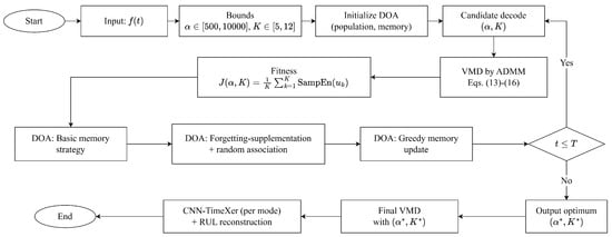
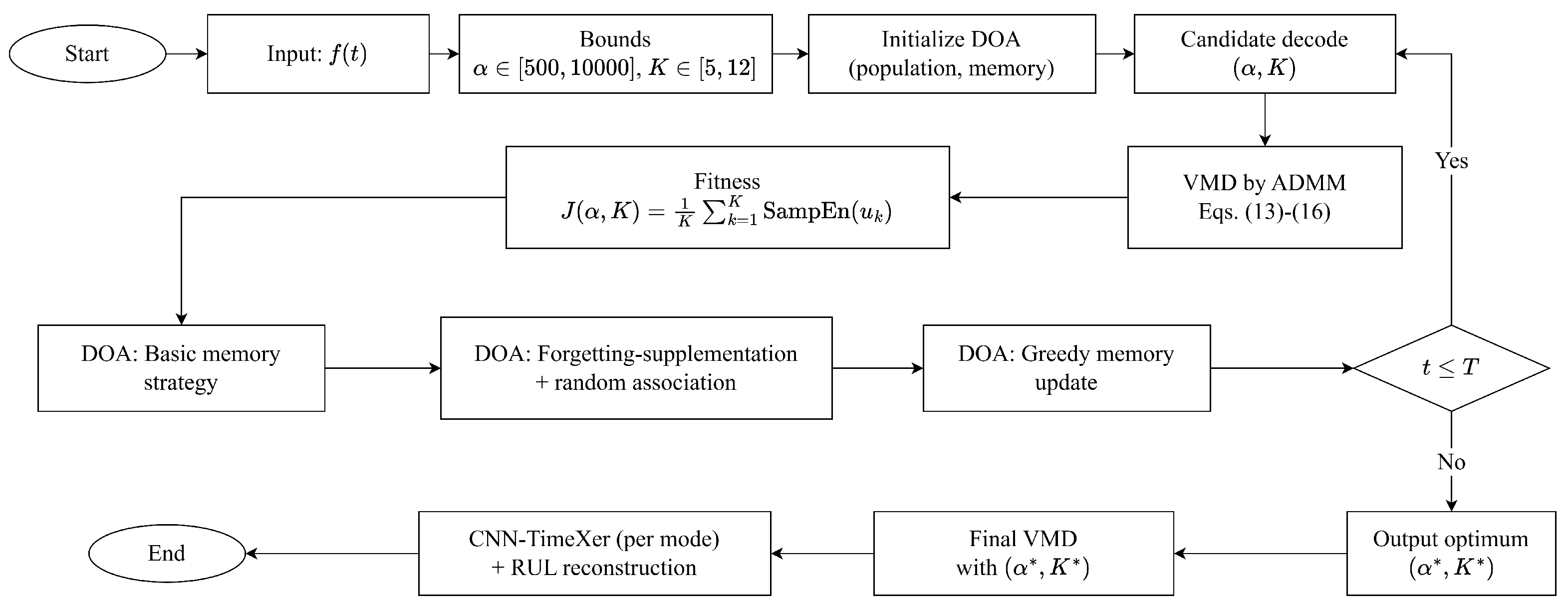
where ${\alpha }_i^t$ is the penalty factor component, $K_i^t$ is the mode-number component, and $D=2$ denotes the dimension of the optimization vector. The overall workflow is shown in Figure 1: DOA iteratively performs candidate decoding, VMD-ADMM decomposition, fitness evaluation, and memory-based state updates until the stopping criterion is satisfied.

Figure 1. Workflow of DOA-based VMD parameter optimization. The outer loop is DOA evolution, and the inner loop evaluates each candidate via VMD-ADMM decomposition and entropy-based fitness computation.

For each candidate pair $(\alpha ,K)$, one full VMD process is executed according to Equations (13)–(16), and then its decomposition quality is evaluated. Although envelope entropy is widely used in VMD parameter tuning [19], this study adopts a predictability-oriented criterion and minimizes the average sample entropy of all modes:

$$\underset{\alpha ,K}{\min }J(\alpha ,K)={\displaystyle \frac{1}{K}}{\displaystyle \sum _{k=1}^K}\mathrm{SampEn}\left(u_k(\alpha ,K)\right),$$

(18)

where $u_k(\alpha ,K)$ is the kth decomposed mode under parameter pair $(\alpha ,K)$. A smaller value of Equation (18) indicates more regular modal dynamics and thus better suitability for the subsequent CNN-TimeXer predictor.

The search ranges are constrained by

$$\alpha \in [500,10000],K\in [5,12],K=\mathrm{round}\left(K\right).$$

(19)

where the penalty factor α is bounded in $[500,10000]$, the mode number K is searched in $[5,12]$, and $\mathrm{round}(·)$ enforces the integer requirement of K. The VMD internal parameters are fixed to $\tau =0$, $DC=0$, $init=1$, and $tol={10}^{-7}$, while the DOA hyper-parameters are set to population size $N=8$ and maximum iteration number $T=30$. Under the bound condition in Equation (19), the final optimal solution is

$$\left({\alpha }^{*},K^{*}\right)=\arg \underset{\alpha ,K}{\min }J(\alpha ,K)$$

(20)

where $\left({\alpha }^{*},K^{*}\right)$ is the optimal VMD parameter pair returned by DOA. The obtained $({\alpha }^{*},K^{*})$ is then used for final decomposition before component-wise prediction and reconstruction. Let N and T denote the DOA population size and maximum iteration number, I the average ADMM iterations in VMD, and L the sequence length. The optimization-stage complexity is summarized as

$${\mathcal{C}}_{\text{DOA-VMD}}=O\left(NT\left({\mathcal{C}}_{\mathrm{VMD}}+{\mathcal{C}}_{\mathrm{SampEn}}\right)\right),{\mathcal{C}}_{\mathrm{VMD}}\approx O\left(IKL\log L\right),$$

(21)

which reflects the outer DOA search and inner VMD-ADMM coupling cost. With fixed VMD internal settings and a bounded decision space, the optimization process remains stable and reproducible.

3. Proposed Predictive Model

3.1. Convolutional Neural Network

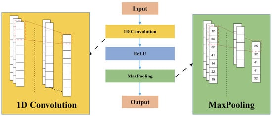
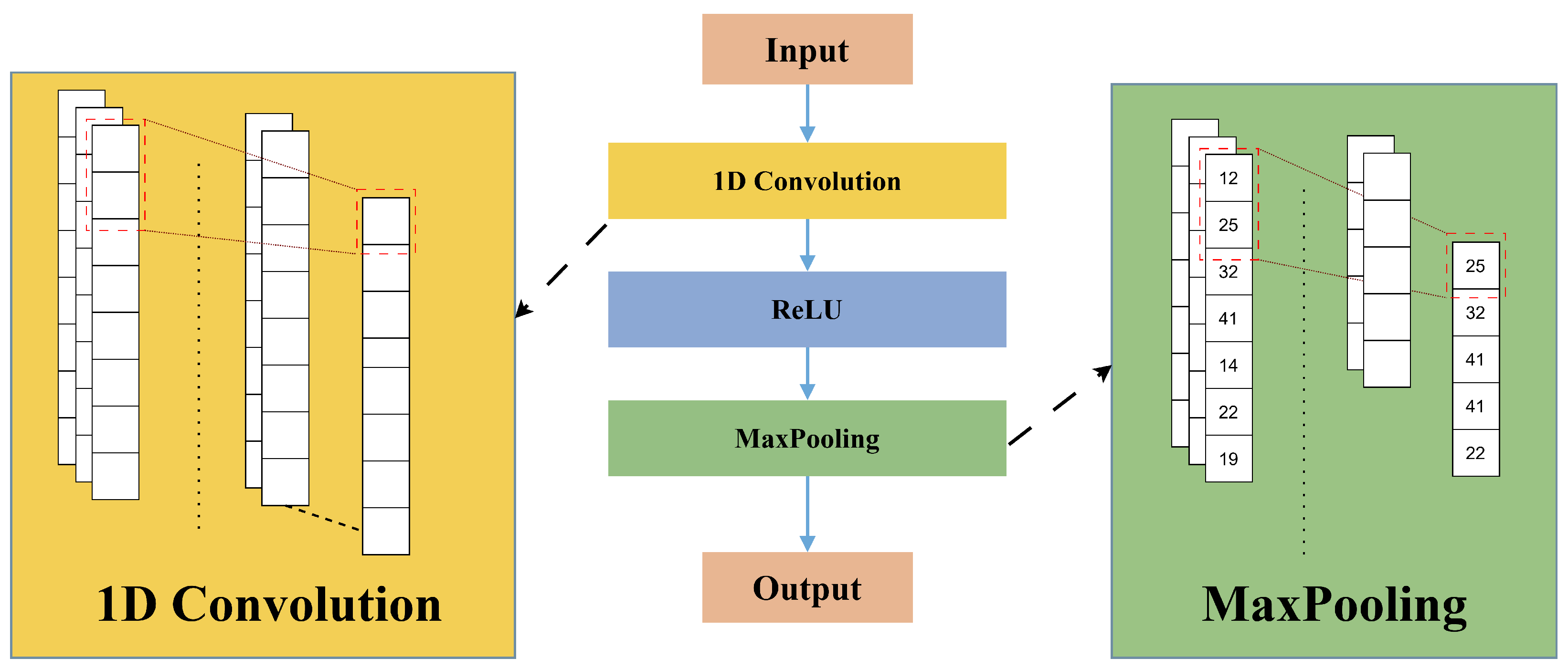
After DOA-VMD decomposition, the original capacity trajectory is represented as multiple relatively band-limited modal components, each preserving local degradation patterns at a specific frequency scale. Although these components are smoother than the raw sequence, they still contain short-range fluctuations and weak local regeneration effects. Therefore, a one-dimensional convolutional neural network (1D-CNN) is introduced to construct a CNN-enhanced exogenous context branch for subsequent TimeXer fusion. The adopted pipeline is illustrated in Figure 2. In the implementation, 1D convolution layers with ReLU are used, and same-padding is applied to preserve sequence length while enhancing local temporal patterns [24].

Figure 2. The 1D-CNN framework used in this study.

Let ${\mathbf{X}}^{\left(k\right)}\in {\mathbb{R}}^{L\times D}$ denote the multivariate input window associated with the kth component, where L is the sequence length and D is the variable dimension. For the lth convolution layer, the cth output channel at position t is computed as

$$z_{t,c}^{(l,k)}={\displaystyle \sum _{m=0}^{q_l-1}}{\displaystyle \sum _{c^{\prime }=1}^{C_{l-1}}}{w}_{m,c^{\prime },c}^{\left(l\right)}{h}_{t+m,c^{\prime }}^{(l-1,k)}+b_c^{\left(l\right)},$$

(22)

where $q_l$ is the kernel size, $C_{l-1}$ is the channel number of layer $l-1$, $w_{m,c^{\prime },c}^{\left(l\right)}$ and $b_c^{\left(l\right)}$ are trainable parameters, and $h^{(0,k)}$ is initialized from ${\mathbf{X}}^{\left(k\right)}$. With same-padding convolution, temporal length is preserved across layers. The nonlinear activation is then applied as

$${\widehat{h}}_{t,c}^{(l,k)}=\varphi \left(z_{t,c}^{(l,k)}\right),\varphi (·)=\mathrm{ReLU}(·),$$

(23)

The stacked convolution–activation pipeline enhances local fluctuation cues while keeping the sequence shape unchanged for subsequent temporal fusion. During training, the CNN parameters are optimized jointly with the downstream modules by minimizing mean squared error, so that the CNN-enhanced exogenous context branch can retain local degradation cues useful for subsequent long-range modeling. For each component, the CNN output is used as enhanced context for the exogenous embedding branch in the subsequent TimeXer module rather than directly replacing endogenous patch tokens.

3.2. TimeXer Network

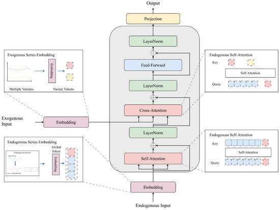
To capture long-range dependency and global degradation evolution, this study adopts an implementation-aligned dual-branch TimeXer-style encoder. The endogenous branch forms patch tokens from the multivariate input sequence, while the exogenous branch embeds CNN-enhanced covariates (with time marks) as contextual tokens. The resulting processing chain is illustrated in Figure 3. This design preserves the sequence-modeling advantages of the TimeXer family and is consistent with multivariate forecasting settings [37].

Figure 3. Implementation-aligned TimeXer architecture for per-component sequence prediction in the proposed framework.

Given a component-wise multivariate input window ${\mathbf{X}}^{\left(k\right)}\in {\mathbb{R}}^{L\times D}$, the endogenous and exogenous branches are formed as

$${\mathbf{Z}}_0^{\left(k\right)}=\mathrm{PatchEmbed}\left({\mathbf{X}}^{\left(k\right)}\right)+\mathbf{P},{\mathbf{C}}^{\left(k\right)}=\mathrm{ExoEmbed}\left({\tilde{\mathbf{X}}}^{\left(k\right)},{\mathbf{M}}^{\left(k\right)}\right),$$

(24)

where ${\tilde{\mathbf{X}}}^{\left(k\right)}$ denotes the CNN-enhanced covariate sequence and ${\mathbf{M}}^{\left(k\right)}$ is the temporal mark embedding. Let ${\mathbf{Z}}_{\mathcal{l}-1}^{\left(k\right)}\in {\mathbb{R}}^{N_p\times d}$ be the endogenous token input of the $\mathcal{l}$th encoder layer. Multi-head self-attention is defined as

$$\mathrm{MSA}\left(\mathbf{Q},\mathbf{K},\mathbf{V}\right)=\mathrm{Concat}\left({\mathrm{head}}_1,\dots ,{\mathrm{head}}_H\right){\mathbf{W}}^O,{\mathrm{head}}_h=\mathrm{Softmax}\left({\displaystyle \frac{{\mathbf{Q}}_h{\mathbf{K}}_h^{\top }}{\sqrt{d_h}}}\right){\mathbf{V}}_h,$$

(25)

with H attention heads and $d_h=d/H$.

Each encoder block first applies endogenous self-attention, then updates the global token through cross-attention with exogenous context, and finally applies feed-forward transformation:

$$\begin{array}{cc}\hfill {\overline{\mathbf{Z}}}_{\mathcal{l}}^{\left(k\right)}& =\mathrm{LN}\left({\mathbf{Z}}_{\mathcal{l}-1}^{\left(k\right)}+\mathrm{MSA}\left({\mathbf{Z}}_{\mathcal{l}-1}^{\left(k\right)}\right)\right),\hfill \\ \hfill {\mathbf{z}}_{g,\mathcal{l}}^{\left(k\right)}& =\mathrm{LN}\left({\overline{\mathbf{z}}}_{g,\mathcal{l}}^{\left(k\right)}+\mathrm{CrossAttn}\left({\overline{\mathbf{z}}}_{g,\mathcal{l}}^{\left(k\right)},{\mathbf{C}}^{\left(k\right)}\right)\right),\hfill \\ \hfill {\mathbf{Z}}_{\mathcal{l}}^{\left(k\right)}& =\mathrm{LN}\left({\tilde{\mathbf{Z}}}_{\mathcal{l}}^{\left(k\right)}+\mathrm{FFN}\left({\tilde{\mathbf{Z}}}_{\mathcal{l}}^{\left(k\right)}\right)\right),\hfill \end{array}$$

(26)

where ${\overline{\mathbf{z}}}_{g,\mathcal{l}}^{\left(k\right)}$ is the global token extracted from ${\overline{\mathbf{Z}}}_{\mathcal{l}}^{\left(k\right)}$, and ${\tilde{\mathbf{Z}}}_{\mathcal{l}}^{\left(k\right)}$ denotes the recombined token sequence obtained by replacing the original global token with ${\mathbf{z}}_{g,\mathcal{l}}^{\left(k\right)}$. Thus, exogenous information is injected mainly through global-token cross-attention. After $L_x$ stacked encoder layers, the prediction head maps the final latent sequence to the component forecast:

$${\widehat{\mathbf{y}}}^{\left(k\right)}=\mathrm{Proj}\left({\mathbf{Z}}_{L_x}^{\left(k\right)}\right),$$

(27)

where ${\widehat{\mathbf{y}}}^{\left(k\right)}$ is the predicted trajectory of the kth mode for subsequent reconstruction in Section 3.3. Related studies using TimeXer and related Transformer-based forecasting architectures in energy, infrastructure, and battery-oriented applications further support the generalization potential of this architecture family [38].

3.3. Component-Wise Capacity Prediction and Reconstruction Process of CNN-TimeXer

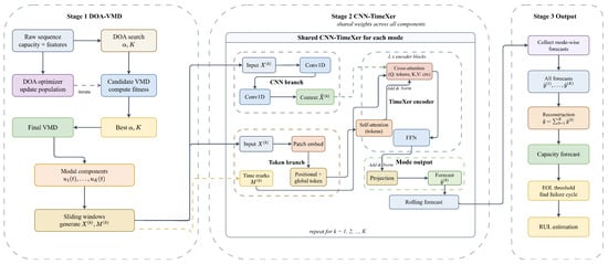
After DOA-VMD decomposition, the original battery degradation trajectory is transformed into K relatively stationary modal components. Instead of predicting the reconstructed signal directly, the proposed framework models each mode separately with the same CNN-TimeXer architecture, as illustrated in Figure 4. This component-wise strategy reduces the learning difficulty caused by mixed-frequency degradation patterns and allows the predictor to focus on modal dynamics at different temporal scales.

Figure 4. Overall framework of the proposed DOA-VMD-CNN-TimeXer method for component-wise battery degradation forecasting and reconstruction.

For the kth decomposed component, a component-specific multivariate input window ${\mathbf{X}}^{\left(k\right)}\in {\mathbb{R}}^{L\times D}$ is fed into two coordinated branches. The CNN branch extracts local fluctuation cues and yields the enhanced exogenous context ${\tilde{\mathbf{X}}}^{\left(k\right)}$, while the TimeXer branch patchifies the original window and encodes temporal marks for contextual interaction. The resulting representations are then integrated by self-attention and global-token cross-attention, and rolling one-step-ahead predictions are generated on sliding windows to form the forecast sequence of each component. The forecast of the kth mode can be expressed at the system level as

$${\widehat{\mathbf{y}}}^{\left(k\right)}={\mathcal{F}}_{\mathrm{CTX}}\left({\mathbf{X}}^{\left(k\right)},{\tilde{\mathbf{X}}}^{\left(k\right)},{\mathbf{M}}^{\left(k\right)}\right),$$

(28)

where ${\mathcal{F}}_{\mathrm{CTX}}(·)$ denotes the complete CNN-TimeXer mapping for one modal component.

After all modal components are predicted, their outputs are collected and superposed to reconstruct the future capacity trajectory, corresponding to the Stage 3 aggregation and reconstruction process in Figure 4:

$$\widehat{\mathbf{y}}={\displaystyle \sum _{k=1}^K}{\widehat{\mathbf{y}}}^{\left(k\right)},$$

(29)

where $\widehat{\mathbf{y}}$ is the reconstructed prediction of the original degradation sequence. In the present study, the reconstructed capacity sequence is directly compared with the measured capacity trajectory in the experimental section, and the model performance is evaluated through capacity-prediction metrics rather than explicit RUL-threshold error. If needed in a downstream application, the reconstructed trajectory can further support RUL estimation by determining the cycle at which the predicted capacity reaches a predefined end-of-life threshold. Accordingly, the proposed method can be summarized as a component-wise CNN-TimeXer prediction pipeline followed by modal reconstruction, which bridges the network design in Section 3 and the experimental verification in Section 4. At the system level, the method follows a compact sequential chain: DOA determines the VMD parameter pair, VMD decomposes the degradation trajectory into modal components, CNN-TimeXer generates component forecasts, and the predicted components are finally superposed to reconstruct the future capacity trajectory.

4. Experiments and Results

4.1. Experimental Configuration

This subsection focuses on the experimental protocol adopted for the proposed framework. To reduce the bias caused by a single train–test partition, two split settings were considered, namely 5:5 and 6:4. Unless otherwise specified, the 5:5 split is treated as the main setting, while the 6:4 split is used as a supplementary robustness check.

For each cell, the chronological sequence was first divided into training and testing segments according to the predefined split ratio, and the subsequent preprocessing and prediction procedures were carried out under this time-ordered setting. The multivariate inputs were normalized by MinMaxScaler, and the DOA-optimized VMD module was then used to generate modal representations for component-wise forecasting. To avoid future-information leakage, VMD was performed after the train–test split under a sliding-window protocol aligned with the model input window, and future values were further blocked by masking in the overall forecasting pipeline. For each modal component, sliding-window samples were constructed from the corresponding component-specific multivariate sequence with an input window length of 30 and a prediction horizon of one step. Temporal covariates generated by the time_features function were fed into the exogenous branch together with the CNN-enhanced modal sequence, and each mode was modeled independently using the same CNN-TimeXer architecture. Accordingly, the present work adopts a rolling trajectory-updating protocol in which newly available observations are sequentially incorporated to support threshold-based RUL inference in an online prognostic setting. The model was implemented in PyTorch 2.7.1 and trained with Adam by minimizing mean squared error. The core hyper-parameter settings are summarized in Table 1, and the DOA-VMD search settings are listed in Table 2. For comparative evaluation, representative Transformer-family models, a linear baseline, and decomposition-based ablation variants were tested under the same data split and prediction protocol. Advanced optimizers such as ALA, QHDBO, and CPO are acknowledged as strong reference methods when positioning the role of DOA in VMD parameter optimization. The quantitative metrics are introduced in the next subsection.

Table 1. Main training hyper-parameters of the proposed DOA-VMD-CNN-TimeXer model.

Module	Parameter	Value
Training	Batch size	32
Training	Epochs	500
Training	Learning rate	0.001
Training	Loss function	MSE
Training	Optimizer	Adam
TimeXer branch	Hidden dimension ($d_{model}$)	128
TimeXer branch	Number of attention heads	8
TimeXer branch	Encoder layers	2
TimeXer branch	Patch length	7
TimeXer branch	Dropout	0.1
CNN branch	Convolution dimension	1D-CNN
CNN branch	Number of convolution layers	2
CNN branch	Kernel size	3

Table 2. DOA-VMD parameter settings used in the experiments.

Item	Value
Optimized variables	Penalty factor α and mode number K
Search range of α	[500, 10,000]
Search range of K	$[5,12]$, with integer rounding
Population size N	8
Maximum iterations T	30

To keep the comparison reproducible and controlled, the CNN-TimeXer hyper-parameters listed in Table 1 were fixed for all CALCE cells and for both train–test splits. The optimization algorithm was applied only at the VMD stage, where the search variables are limited to the mode number K and penalty factor α. Jointly optimizing both decomposition parameters and CNN-TimeXer hyper-parameters would require repeated end-to-end retraining and substantially higher training cost; therefore, the present study keeps the predictor hyper-parameters fixed and leaves optimization-based CNN-TimeXer hyper-parameter tuning for future work.

4.2. Lithium Battery Experimental Data Introduction and Analysis

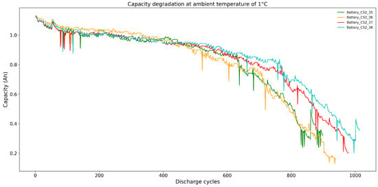
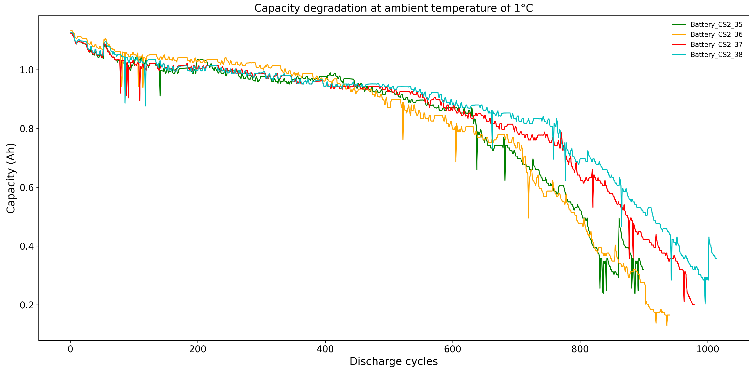
The CALCE lithium-ion battery degradation dataset was adopted for experimental evaluation, and four representative cells, namely CS35, CS36, CS37, and CS38, were selected. This subsection is limited to the data summary and degradation-trajectory analysis. The basic data usage is summarized in Table 3, and the corresponding capacity degradation trajectories are shown in Figure 5.

Table 3. Summary of the CALCE battery data used in this study.

Cell	Usable Cycles	Input Variables	Target
CS35	899	Cycle-level multivariate degradation indicators	Capacity
CS36	940	Cycle-level multivariate degradation indicators	Capacity
CS37	979	Cycle-level multivariate degradation indicators	Capacity
CS38	1014	Cycle-level multivariate degradation indicators	Capacity

Figure 5. Capacity degradation trajectories of the CALCE lithium-ion battery cells used in this study.

Following the local CALCE preprocessing routine, the raw records were reorganized into battery-wise chronological sequences, from which cycle-level indicators were extracted from voltage, current, time, energy, and resistance measurements. Local abnormal samples were then removed by a 3σ filtering strategy, and the retained cycle summaries were assembled into battery-wise feature tables. On this basis, the selected degradation-sensitive variables were reorganized into a model-ready multivariate sequence, in which Target denotes the capacity to be predicted.

The resulting multivariate inputs can be grouped into four categories, while capacity is taken as the prediction target: charging-time descriptors, energy-related descriptors, voltage-dynamic descriptors, and degradation-sensitive electrochemical indicators. Representative variables include constant-current/constant-voltage charging durations and their ratio, charge/discharge energy and energy efficiency, voltage response-rate and transition-time features, and electrochemical health indicators such as resistance and incremental-capacity peak characteristics. These variables are treated here as cycle-level degradation indicators derived from charge/discharge behavior and battery health evolution. They reflect complementary aspects of battery aging, including charge-transfer behavior, energy conversion deterioration, dynamic voltage response, and internal electrochemical evolution. Accordingly, the adopted feature set is intended to characterize degradation from multiple coupled perspectives rather than to rely on a single observable quantity.

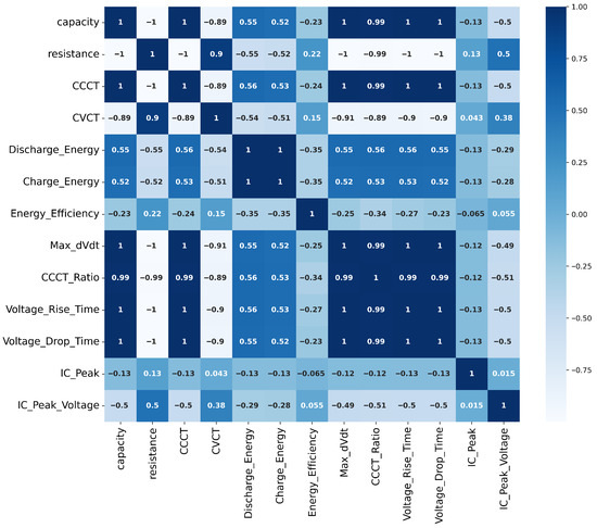
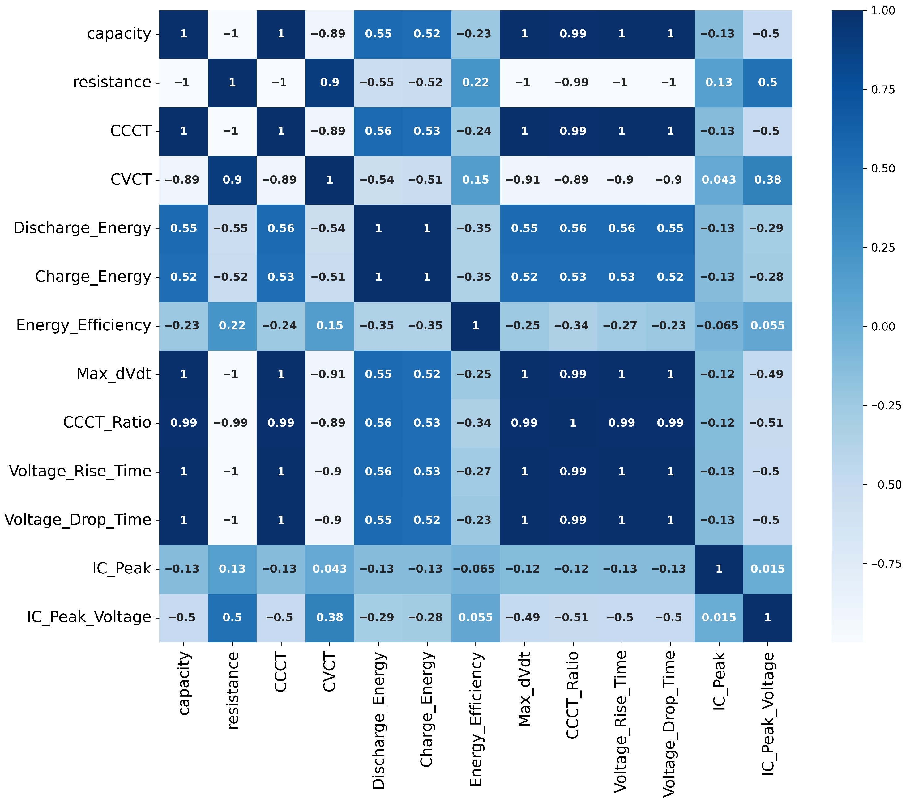
To evaluate the relevance of the constructed indicators, Pearson correlation analysis was performed on the processed multivariate data, as shown in Figure 6. Several engineered variables exhibit clear association with the target capacity, while noticeable inter-feature correlation suggests that battery aging is governed by coupled electrochemical and operational mechanisms rather than by a single observable quantity. This result supports the use of multivariate sequence modeling instead of a capacity-only univariate predictor.

Figure 6. Pearson correlation analysis of the constructed multivariate degradation indicators.

As shown in Figure 5, all four cells exhibit an overall capacity-fading trend, while still presenting local fluctuations and evident cell-to-cell heterogeneity. This behavior indicates that the degradation sequence is nonlinear and non-stationary, which increases the difficulty of direct forecasting. This observation provides the data-level motivation for the subsequent DOA-VMD-CNN-TimeXer framework, in which decomposition is introduced to simplify the degradation signal before component-wise forecasting.

4.3. Evaluation Metrics

To quantitatively assess the prediction accuracy of the proposed method, the reconstructed capacity trajectory is compared with the measured capacity sequence by four widely used regression metrics, namely MAPE, R², MSE, and RMSE. In battery prognosis studies, these trajectory-level metrics are commonly used to evaluate the quality of degradation modeling, which in turn provides the basis for subsequent threshold-based RUL inference. Let $y_i$ and ${\widehat{y}}_i$ denote the measured and predicted capacities of the ith cycle, respectively, $\overline{y}$ denote the mean of the measured capacity sequence, and N denote the number of evaluated samples. The corresponding metrics are defined as follows:

$$\mathrm{MAPE}={\displaystyle \frac{1}{N}}{\displaystyle \sum _{i=1}^N}\left|{\displaystyle \frac{y_i-{\widehat{y}}_i}{y_i}}\right|\times 100\%$$

(30)

$$R^2=1-{\displaystyle \frac{{\sum }_{i=1}^N{(y_i-{\widehat{y}}_i)}^2}{{\sum }_{i=1}^N{(y_i-\overline{y})}^2}}$$

(31)

$$\mathrm{MSE}={\displaystyle \frac{1}{N}}{\displaystyle \sum _{i=1}^N}{(y_i-{\widehat{y}}_i)}^2$$

(32)

$$\mathrm{RMSE}=\sqrt{{\displaystyle \frac{1}{N}}{\sum }_{i=1}^N{(y_i-{\widehat{y}}_i)}^2}$$

(33)

Among them, MAPE reflects the relative deviation, MSE and RMSE quantify the absolute error magnitude, and R² measures the goodness of fit between the predicted and observed capacity trajectories. Therefore, lower values of MAPE, MSE, and RMSE and a higher value of R² indicate better prediction performance. In the present study, these metrics are used to evaluate the reconstructed degradation trajectory rather than to directly quantify threshold-crossing RUL error.

4.4. DOA-VMD Analysis and Prediction of Components

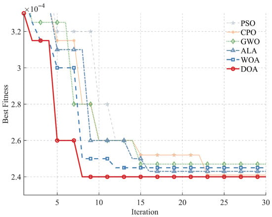
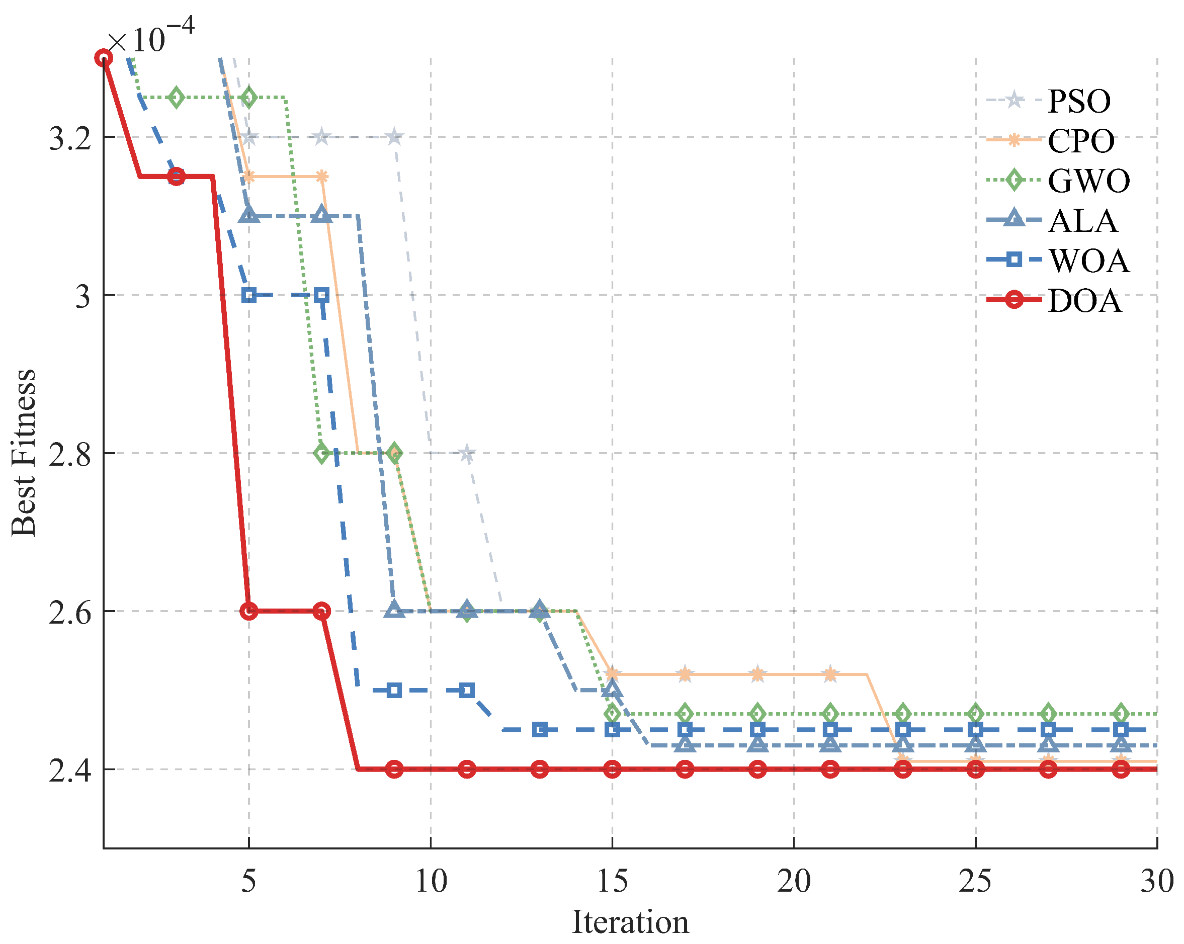
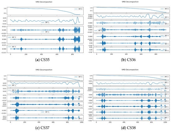
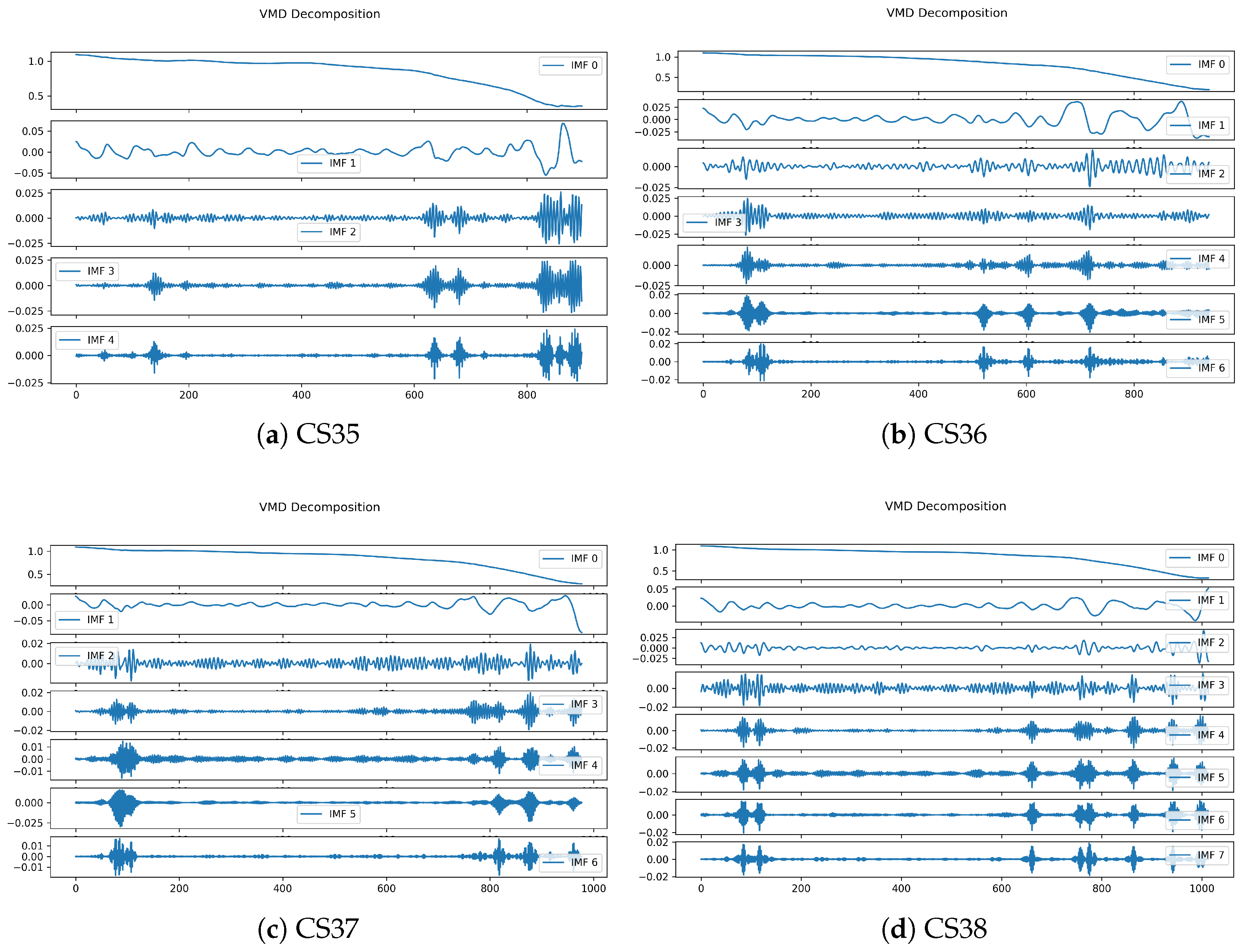
The convergence behavior of the optimization stage is shown in Figure 7. The results indicate that the compared optimization algorithms converge stably under the adopted VMD parameter-tuning setting. In Figure 8, IMF 0 mainly preserves the global degradation trend, whereas IMF 1–4 capture fluctuation components at different temporal scales. As shown in Figure 8a–d, the original battery capacity sequences can be separated by DOA-VMD into modal components with clearly different temporal characteristics. The low-frequency components mainly preserve the global degradation tendency and therefore describe the long-term capacity-fading trajectory, whereas the high-frequency components retain local oscillations, short-term regeneration-like fluctuations, and random disturbances. This decomposition is meaningful for lithium-ion battery prognosis because the raw degradation sequence is non-stationary and contains mixed-scale dynamics that are difficult to model directly in a single predictor. After decomposition, each sub-series becomes more regular in its dominant temporal pattern, which provides a more suitable input form for subsequent component-wise forecasting.

Figure 7. Convergence curves of different optimization algorithms for VMD parameter tuning, where the best fitness is plotted against the iteration number.

Figure 8. DOA-VMD decomposition results of the four CALCE battery capacity sequences. The legends in each subfigure identify IMF 0–IMF n, where IMF 0 mainly represents the low-frequency degradation trend and the remaining IMFs describe fluctuation components at different temporal scales.

Because the degradation characteristics are not identical across cells, the optimal VMD parameter pair returned by DOA is also cell-dependent. Table 4 lists the final parameter settings used for the four CALCE batteries. It can be seen that DOA assigns different combinations of mode number K and penalty factor α to CS35–CS38, indicating that the decomposition stage is adaptively matched to the complexity and fluctuation intensity of each degradation trajectory rather than relying on a uniform empirical configuration.

Table 4. DOA-optimized VMD parameter settings for different CALCE battery cells.

Parameter	CS-35	CS-36	CS-37	CS-38
Mode number K	5	7	7	8
Penalty factor α	1102	1202	1140	1060

The results in Table 4 further explain why the proposed framework emphasizes adaptive decomposition before prediction. For example, CS38 is decomposed into more modes than CS35, which suggests that its degradation sequence contains relatively richer multi-scale variation, whereas the penalty factors remain within a comparable range to maintain stable band-limited separation. On this basis, the subsequent CNN-TimeXer predictor can learn local and global temporal patterns from modal components generated under more suitable decomposition conditions.

To further illustrate the optimization behavior of DOA during VMD parameter tuning, Figure 7 presents the convergence curves of different optimizers. It can be observed that DOA reduces the fitness value more rapidly in the early iterations and reaches a lower stable level than PSO, CPO, GWO, ALA, and WOA under the evaluated setting. In particular, the DOA curve shows a pronounced fitness decrease within the first several iterations and then becomes nearly flat after about the eighth iteration, indicating that the search process can identify a high-quality parameter region with relatively fast convergence. This behavior is consistent with the role of DOA in the proposed framework, namely improving the efficiency and effectiveness of VMD parameter adaptation before the subsequent component-wise CNN-TimeXer prediction stage.

The decomposition results corresponding to the parameter settings in Table 4 are illustrated in Figure 8a–d, which are arranged as subfigures in Figure 8. These subfigures show that, after DOA-based parameter adaptation, each cell can be decomposed into a set of modal components with relatively clear frequency stratification. In general, the low-frequency modes capture the smooth long-term degradation trend, while the higher-frequency modes retain local fluctuations and regeneration-like perturbations. This result further confirms that the optimized VMD stage provides a more structured signal representation for subsequent component-wise CNN-TimeXer prediction.

Based on this decomposition result, the proposed predictor performs component-level modeling rather than direct end-to-end regression on the raw sequence. In this process, the CNN branch is mainly responsible for extracting local fluctuation patterns and short-range shape information from each modal component, while the TimeXer branch captures long-range temporal dependencies and cross-window evolution trends. Compared with predicting the original non-stationary trajectory directly, the modal prediction strategy reduces the complexity of the learning target and allows the model to focus on structured information at different temporal scales. After one-step rolling prediction is completed for each component, the final capacity trajectory is reconstructed by summing the modal forecasts, thereby linking local modal learning back to the global degradation process.

From the representative decomposition and reconstruction results, it can be qualitatively observed that the proposed strategy provides a clearer bridge between degradation characterization and sequence prediction. The decomposition stage simplifies the signal structure, while the CNN-TimeXer predictor learns complementary temporal patterns from the simplified components. Therefore, the performance gain of the proposed framework should not be understood as the isolated contribution of a single module, but rather as the joint effect of optimized decomposition and component-wise temporal modeling. This point is further examined in the following ablation and comparative experiments.

4.5. Ablation Experiment

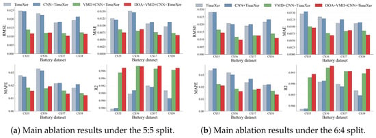
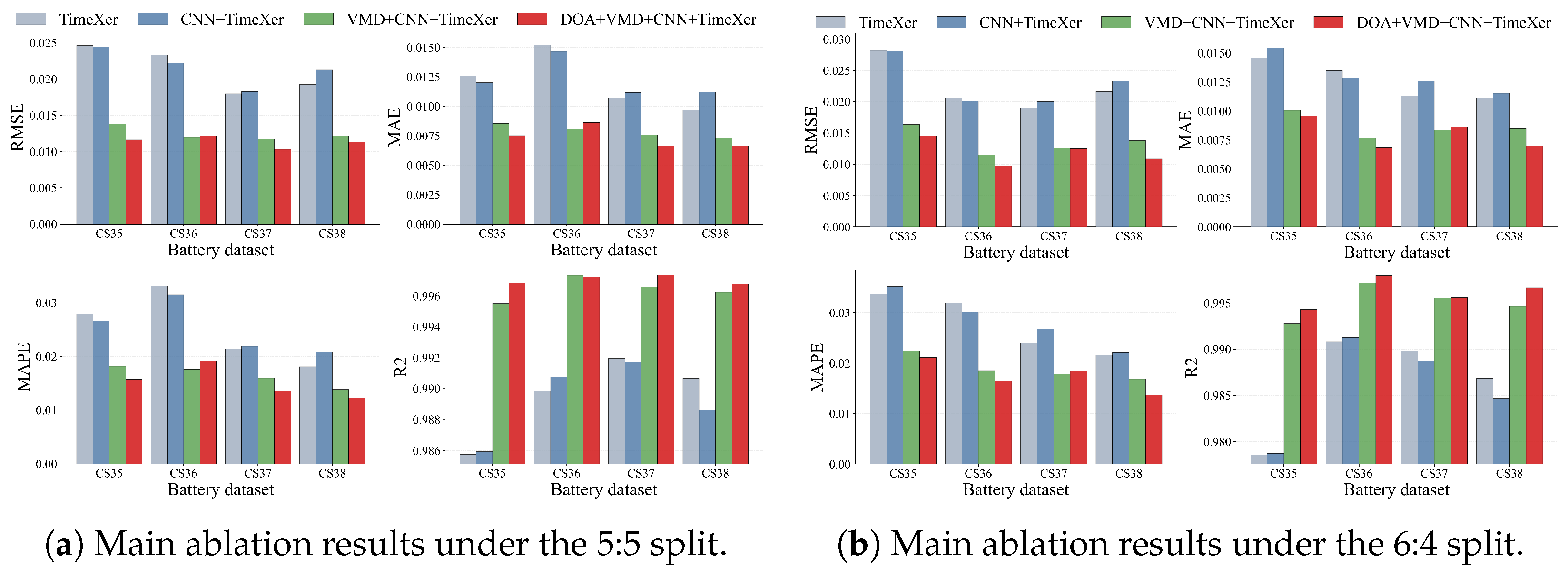
To verify whether the performance of the proposed framework originates from the complete modeling chain rather than from a single architectural enhancement, a main ablation study was conducted under both the 5:5 and 6:4 train–test splits. As summarized in Table 5 and Table 6 and visualized in Figure 9, four model variants are compared, namely the plain TimeXer predictor, CNN+TimeXer, VMD+CNN+TimeXer, and the full DOA-VMD-CNN-TimeXer model. This progressive design makes it possible to isolate the effects of direct CNN enhancement, decomposition-assisted component-wise modeling, and adaptive DOA-based parameter optimization.

Table 5. Main ablation results of different model variants under the 5:5 split. Lower MAPE, MSE, and RMSE and higher R² indicate better performance.

Cell	Model	MAPE (%)	R2	MSE	RMSE
CS35	TimeXer	2.783478	0.985741	0.000607	0.024634
CS35	CNN+TimeXer	2.667013	0.985916	0.000599	0.024482
CS35	VMD+CNN+TimeXer	1.815481	0.995488	0.000192	0.013851
CS35	DOA-VMD-CNN-TimeXer	1.575248	0.996808	0.000136	0.011650
CS36	TimeXer	3.305005	0.989853	0.000543	0.023299
CS36	CNN+TimeXer	3.147280	0.990769	0.000494	0.022223
CS36	VMD+CNN+TimeXer	1.761852	0.997329	0.000143	0.011954
CS36	DOA-VMD-CNN-TimeXer	1.916656	0.997237	0.000148	0.012158
CS37	TimeXer	2.142538	0.991953	0.000324	0.018006
CS37	CNN+TimeXer	2.187737	0.991695	0.000335	0.018292
CS37	VMD+CNN+TimeXer	1.593849	0.996590	0.000137	0.011717
CS37	DOA-VMD-CNN-TimeXer	1.350767	0.997356	0.000106	0.010316
CS38	TimeXer	1.810034	0.990662	0.000370	0.019248
CS38	CNN+TimeXer	2.080160	0.988593	0.000453	0.021274
CS38	VMD+CNN+TimeXer	1.387822	0.996251	0.000149	0.012196
CS38	DOA-VMD-CNN-TimeXer	1.228672	0.996757	0.000129	0.011343

Table 6. Main ablation results of different model variants under the 6:4 split. Lower MAPE, MSE, and RMSE and higher R² indicate better performance.

Cell	Model	MAPE (%)	R2	MSE	RMSE
CS35	TimeXer	3.372238	0.978584	0.000795	0.028204
CS35	CNN+TimeXer	3.518499	0.978720	0.000790	0.028114
CS35	VMD+CNN+TimeXer	2.239852	0.992769	0.000269	0.016388
CS35	DOA-VMD-CNN-TimeXer	2.114026	0.994317	0.000211	0.014528
CS36	TimeXer	3.201371	0.990851	0.000426	0.020649
CS36	CNN+TimeXer	3.022825	0.991291	0.000406	0.020146
CS36	VMD+CNN+TimeXer	1.857122	0.997146	0.000133	0.011534
CS36	DOA-VMD-CNN-TimeXer	1.370099	0.996669	0.000119	0.010887
CS37	TimeXer	2.392097	0.989865	0.000360	0.018974
CS37	CNN+TimeXer	2.675705	0.988702	0.000401	0.020034
CS37	VMD+CNN+TimeXer	1.781297	0.995548	0.000158	0.012576
CS37	DOA-VMD-CNN-TimeXer	1.851480	0.995598	0.000156	0.012506
CS38	TimeXer	2.162346	0.986861	0.000468	0.021622
CS38	CNN+TimeXer	2.210566	0.984686	0.000545	0.023344
CS38	VMD+CNN+TimeXer	1.685164	0.994652	0.000190	0.013795
CS38	DOA-VMD-CNN-TimeXer	1.451818	0.996351	0.000130	0.011394

Figure 9. Main ablation comparison of different model variants under the two train–test splits. Each panel summarizes cell-wise RMSE, MSE, MAPE (%), and R² for TimeXer, CNN+TimeXer, VMD+CNN+TimeXer, and DOA-VMD-CNN-TimeXer.

The ablation results reveal that simply adding a CNN front-end to the raw TimeXer predictor does not consistently improve performance when the original non-stationary capacity trajectory is modeled directly. Averaged over the four cells, the RMSE changes from 0.021296 to 0.021568 under the 5:5 split and from 0.022362 to 0.022909 under the 6:4 split, while the corresponding average R² values decrease slightly from 0.989552 to 0.989243 and from 0.986540 to 0.985850, respectively. This result indicates that local convolution alone is insufficient to resolve the mixed-scale fluctuations and long-range degradation coupling contained in the raw sequence.

In contrast, decomposition-assisted component-wise modeling brings the dominant gain. When VMD and CNN are introduced together, the prediction target is transferred from the raw trajectory to modal components with clearer temporal structure, and the CNN branch can focus on local fluctuation cues within each component before TimeXer captures long-range evolution. Relative to TimeXer, the average RMSE decreases from 0.021296 to 0.012430 under the 5:5 split and from 0.022362 to 0.013573 under the 6:4 split, corresponding to reductions of 41.64% and 39.30%, respectively. Meanwhile, the average MAPE decreases from 2.5103% to 1.6398% under the 5:5 split and from 2.7820% to 1.8909% under the 6:4 split. The bar charts in Figure 9a,b further show that this improvement is consistently reflected across all four cells and across the reported MSE, RMSE, MAPE (%), and R² metrics.

The comparison between VMD+CNN+TimeXer and the full DOA-VMD-CNN-TimeXer configuration further supports the value of adaptive decomposition at the overall-performance level. On average, DOA optimization reduces the RMSE by a further 8.55% under the 5:5 split and 9.17% under the 6:4 split relative to the manually configured VMD+CNN+TimeXer model, while the average MAPE decreases by 7.43% and 10.26%, respectively, and the average R² increases by 0.000625 and 0.000705. The gain is not numerically uniform on every single cell, which is also informative. Under the 5:5 split, CS36 slightly favors the manually configured VMD+CNN+TimeXer setting, with RMSE changing from 0.011954 to 0.012158 and MAPE from 1.7619% to 1.9167%. Under the 6:4 split, the difference on CS37 is marginal, with RMSE changing only from 0.012576 to 0.012506, while the MAPE increases slightly from 1.7813% to 1.8515%. Therefore, the contribution of DOA in the present study should be interpreted as improving the overall average accuracy and cross-split robustness of the framework under the evaluated settings, rather than guaranteeing a strict per-cell improvement in every case.

Overall, the ablation analysis supports a structured interpretation of the model design. CNN enhancement alone does not solve the difficulty of raw non-stationary sequence forecasting, whereas VMD substantially improves signal separability and creates a more suitable basis for component-wise prediction. On top of that, DOA mainly strengthens the average accuracy–robustness trade-off of the decomposition-assisted framework, even though its gain is not numerically uniform for every individual cell. Accordingly, the DOA-VMD-CNN-TimeXer framework provides the best overall performance because it integrates decomposition quality, local feature extraction, and long-range temporal modeling into a unified forecasting pipeline.

4.6. Model Comparison

For clarity and reproducibility, the key hyper-parameter settings of the comparative models are summarized in Table 7. To avoid an excessively large table, only the key settings that differentiate the model structures are listed. Unless otherwise stated, the compared models were trained with a unified input length of 30 and 500 training epochs. For the baseline scripts implemented under the same forecasting framework (FEDformer, NTSformer, Informer, TimeNet, iTransformer, TimeXer, DLinear, and PatchTST), the common training protocol used Adam, a batch size of 32, a one-step prediction horizon, ReduceLROnPlateau learning-rate scheduling, and an early-stopping ratio of 0.2. In addition, most Transformer-family baselines shared the same backbone-level settings, namely $d_{\mathrm{model}}=64$, eight attention heads, encoder/decoder layers = 2/1, and $d_{ff}=64$. Most of these models were trained with a learning rate of 0.001, while the standalone Transformer baseline followed its own implementation setting with a batch size of 64 and a learning rate of 0.0001. The proposed DOA-VMD-CNN-TimeXer model adopted the same core CNN-TimeXer training setup as described in Section 4.1, while its DOA-VMD search settings are separately reported in Table 2.

Table 7. Key hyper-parameter settings of the comparative models used in Table 8 and Table 9.

Model	Model-Specific Setting
Transformer	heads = 4; blocks = 3; dropout = 0.01; batch size = 64; learning rate = 0.0001
FEDformer	moving average = 29
NTSformer	projector hidden dims $=[64,64]$; projector layers = 2
Informer	distillation enabled
TimeNet	top-k = 5; number of kernels = 6
iTransformer	distillation enabled
TimeXer	patch length = 7; stride = 4
DLinear	linear decomposition predictor; moving average = 1
PatchTST	patch length = 16; stride = 8
DOA-VMD-CNN-TimeXer	two 1D convolution layers; patch length = 7; stride = 4

To evaluate the overall effectiveness of the proposed framework, the full DOA-VMD-CNN-TimeXer model is compared with representative baseline methods under two train–test split settings. Table 8 reports the primary 5:5 results and shows that the proposed method achieves the lowest RMSE on all four tested cells, namely 0.011650, 0.012158, 0.010316, and 0.011343 for CS35–CS38, respectively. The corresponding R² values are 0.996808, 0.997237, 0.997356, and 0.996757, indicating strong agreement between predicted and observed degradation trajectories. Relative to the strongest baseline under the same setting, which is PatchTST for all four cells, the RMSE is further reduced by 50.2%, 32.8%, 32.3%, and 41.1%, respectively. After further adding three decomposition-assisted recurrent baselines, namely CEEMDAN-LSTM, EMD-LSTM, and VMD-LSTM, the proposed method still preserves the best performance on all four cells. Compared with the strongest newly added LSTM-type competitor on each cell, the RMSE is further reduced by 66.0%, 68.0%, 59.8%, and 53.9% under the 5:5 split, which further highlights the advantage of the proposed DOA-VMD-CNN-TimeXer framework over conventional decomposition-plus-LSTM routes. These gains indicate that the proposed framework provides a consistent accuracy advantage on the tested CALCE cells under the primary split.

Table 8. Comparison of different methods under the 5:5 train–test split. Lower MAPE, MSE, and RMSE and higher R² indicate better performance.

Cell	Model	MAPE (%)	R2	MSE	RMSE
CS35	Transformer	5.432375	0.963780	0.001535	0.039177
CS35	FEDformer	4.092794	0.968228	0.001352	0.036770
CS35	NTSformer	3.891682	0.975523	0.001042	0.032274
CS35	Informer	3.643285	0.977244	0.000968	0.031119
CS35	TimeNet	3.497031	0.978381	0.000920	0.030332
CS35	iTransformer	2.814859	0.983754	0.000691	0.026294
CS35	TimeXer	2.783478	0.985741	0.000607	0.024634
CS35	DLinear	2.807035	0.986705	0.000566	0.023786
CS35	PatchTST	2.442531	0.987148	0.000547	0.023386
CS35	CEEMDAN-LSTM	4.058697	0.972181	0.001177	0.034305
CS35	EMD-LSTM	4.697767	0.965984	0.001439	0.037934
CS35	VMD-LSTM	4.739762	0.966388	0.001422	0.037708
CS35	DOA-VMD-CNN-TimeXer	1.575248	0.996808	0.000136	0.011650
CS36	Transformer	14.463192	0.859779	0.007455	0.086343
CS36	FEDformer	20.435399	0.822095	0.009517	0.097557
CS36	NTSformer	3.632773	0.989846	0.000543	0.023307
CS36	Informer	3.935818	0.988759	0.000601	0.024522
CS36	TimeNet	3.105727	0.991668	0.000446	0.021113
CS36	iTransformer	2.560886	0.992570	0.000397	0.019937
CS36	TimeXer	3.305005	0.989853	0.000543	0.023299
CS36	DLinear	4.086267	0.990461	0.000510	0.022590
CS36	PatchTST	2.313864	0.993889	0.000327	0.018081
CS36	CEEMDAN-LSTM	5.967776	0.968597	0.001667	0.040827
CS36	EMD-LSTM	4.905811	0.972625	0.001453	0.038118
CS36	VMD-LSTM	7.977945	0.945757	0.002879	0.053657
CS36	DOA-VMD-CNN-TimeXer	1.916656	0.997237	0.000148	0.012158
CS37	Transformer	27.969207	0.355905	0.025702	0.160318
CS37	FEDformer	3.654966	0.977463	0.000908	0.030133
CS37	NTSformer	3.250713	0.987322	0.000511	0.022600
CS37	Informer	3.156224	0.987521	0.000503	0.022423
CS37	TimeNet	3.154140	0.987665	0.000497	0.022293
CS37	iTransformer	2.073982	0.991161	0.000356	0.018871
CS37	TimeXer	2.142538	0.991953	0.000324	0.018006
CS37	DLinear	1.876605	0.993165	0.000275	0.016595
CS37	PatchTST	1.503503	0.994246	0.000232	0.015226
CS37	CEEMDAN-LSTM	3.011214	0.983455	0.000659	0.025673
CS37	EMD-LSTM	3.638823	0.979972	0.000798	0.028246
CS37	VMD-LSTM	11.092163	0.888454	0.004444	0.066660
CS37	DOA-VMD-CNN-TimeXer	1.350767	0.997356	0.000106	0.010316
CS38	Transformer	17.022631	0.732697	0.010572	0.102820
CS38	FEDformer	4.367802	0.972418	0.001094	0.033080
CS38	NTSformer	3.303899	0.981063	0.000751	0.027410
CS38	Informer	3.082740	0.981927	0.000717	0.026777
CS38	TimeNet	3.187846	0.981181	0.000747	0.027324
CS38	iTransformer	1.765263	0.990147	0.000391	0.019771
CS38	TimeXer	1.810034	0.990662	0.000370	0.019248
CS38	DLinear	1.774109	0.990315	0.000384	0.019602
CS38	PatchTST	1.627116	0.990663	0.000370	0.019247
CS38	CEEMDAN-LSTM	2.655795	0.984686	0.000607	0.024638
CS38	EMD-LSTM	3.203013	0.980451	0.000775	0.027837
CS38	VMD-LSTM	7.218782	0.944051	0.002218	0.047093
CS38	DOA-VMD-CNN-TimeXer	1.228672	0.996757	0.000129	0.011343

Table 9 provides a supplementary check under the 6:4 split. Under this setting, DOA-VMD-CNN-TimeXer still achieves the lowest RMSE on all four tested cells, namely 0.014528, 0.010887, 0.012506, and 0.011394 for CS35–CS38, respectively, while all corresponding R² values remain above 0.994. Relative to the strongest baseline under the same setting, which is PatchTST for all four cells, the RMSE is further reduced by 44.8%, 49.1%, 24.2%, and 46.8%, respectively. The same superiority is maintained after introducing CEEMDAN-LSTM, EMD-LSTM, and VMD-LSTM into Table 9. In particular, compared with the strongest newly added decomposition-LSTM baseline on each cell, the RMSE remains lower by 45.4%, 70.8%, 47.0%, and 59.1%, respectively, which indicates that the benefit of the proposed framework is robust across both data-split settings rather than being specific to one partition. Therefore, the observed advantage of the proposed model is not limited to the primary 5:5 partition and is also reflected under the supplementary split.

Table 9. Comparison of different methods under the 6:4 train–test split. Lower MAPE, MSE, and RMSE and higher R² indicate better performance.

Cell	Model	MAPE (%)	R2	MSE	RMSE
CS35	Transformer	9.076730	0.920801	0.002935	0.054175
CS35	FEDformer	5.463415	0.954244	0.001699	0.041225
CS35	NTSformer	4.713563	0.965470	0.001283	0.035812
CS35	Informer	4.546203	0.967820	0.001195	0.034572
CS35	TimeNet	4.482593	0.967393	0.001211	0.034801
CS35	iTransformer	3.385704	0.976879	0.000859	0.029305
CS35	TimeXer	3.372238	0.978584	0.000795	0.028204
CS35	DLinear	3.625323	0.979722	0.000753	0.027444
CS35	PatchTST	2.963391	0.981342	0.000693	0.026325
CS35	CEEMDAN-LSTM	3.205183	0.980661	0.000713	0.026705
CS35	EMD-LSTM	3.898822	0.974177	0.000952	0.030858
CS35	VMD-LSTM	6.022413	0.954996	0.001660	0.040738
CS35	DOA-VMD-CNN-TimeXer	2.114026	0.994317	0.000211	0.014528
CS36	Transformer	7.471326	0.926241	0.002615	0.051141
CS36	FEDformer	4.568228	0.958986	0.001459	0.038202
CS36	NTSformer	4.008523	0.972712	0.000971	0.031161
CS36	Informer	3.650949	0.975623	0.000867	0.029452
CS36	TimeNet	3.814419	0.974095	0.000922	0.030361
CS36	iTransformer	2.348032	0.984775	0.000542	0.023275
CS36	TimeXer	2.162346	0.986861	0.000468	0.021622
CS36	DLinear	2.018584	0.986966	0.000464	0.021535
CS36	PatchTST	1.961891	0.987121	0.000458	0.021407
CS36	CEEMDAN-LSTM	4.072000	0.960837	0.001387	0.037247
CS36	EMD-LSTM	4.631425	0.958371	0.001475	0.038401
CS36	VMD-LSTM	5.310049	0.952677	0.001676	0.040943
CS36	DOA-VMD-CNN-TimeXer	1.370099	0.996669	0.000119	0.010887
CS37	Transformer	22.712768	0.593908	0.014284	0.119515
CS37	FEDformer	3.630645	0.981524	0.000656	0.025620
CS37	NTSformer	3.909640	0.982321	0.000628	0.025061
CS37	Informer	4.198869	0.979041	0.000745	0.027286
CS37	TimeNet	3.696795	0.982938	0.000606	0.024620
CS37	iTransformer	2.237852	0.990000	0.000355	0.018848
CS37	TimeXer	2.392097	0.989865	0.000360	0.018974
CS37	DLinear	1.954888	0.991200	0.000313	0.017681
CS37	PatchTST	1.678243	0.992333	0.000272	0.016504
CS37	CEEMDAN-LSTM	2.788026	0.984062	0.000559	0.023642
CS37	EMD-LSTM	3.938734	0.977603	0.000785	0.028027
CS37	VMD-LSTM	9.560546	0.917324	0.002900	0.053848
CS37	DOA-VMD-CNN-TimeXer	1.851480	0.995598	0.000156	0.012506
CS38	Transformer	36.939901	−0.182435	0.041927	0.204761
CS38	FEDformer	5.240533	0.950408	0.001765	0.042007
CS38	NTSformer	3.929135	0.972523	0.000978	0.031268
CS38	Informer	3.641972	0.974969	0.000891	0.029844
CS38	TimeNet	3.805822	0.973762	0.000934	0.030556
CS38	iTransformer	2.173210	0.986787	0.000470	0.021683
CS38	TimeXer	2.227607	0.986537	0.000479	0.021887
CS38	DLinear	2.385866	0.985752	0.000507	0.022516
CS38	PatchTST	1.897397	0.987087	0.000459	0.021436
CS38	CEEMDAN-LSTM	3.293004	0.977961	0.000781	0.027941
CS38	EMD-LSTM	4.087577	0.970126	0.001058	0.032531
CS38	VMD-LSTM	13.675259	0.824145	0.006229	0.078927
CS38	DOA-VMD-CNN-TimeXer	1.451818	0.996351	0.000130	0.011394

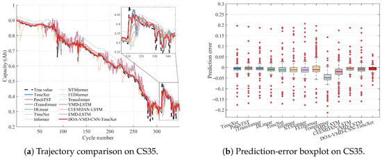
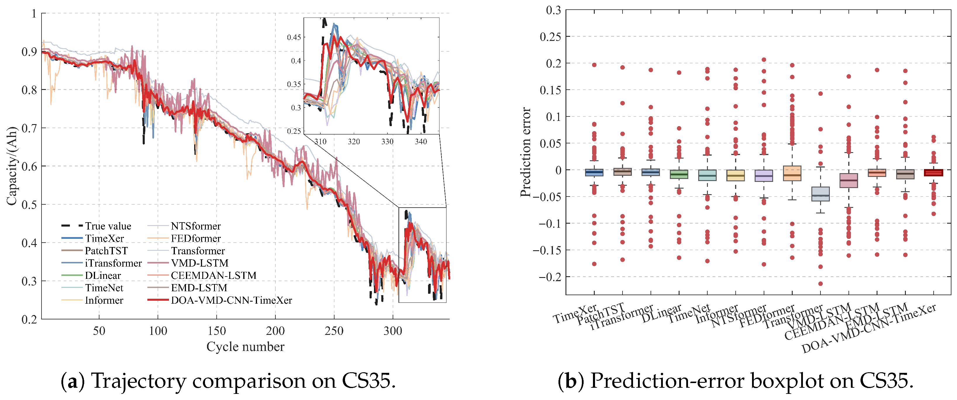
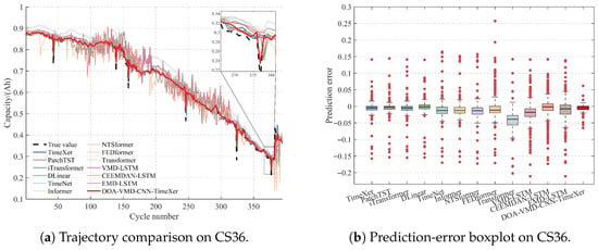
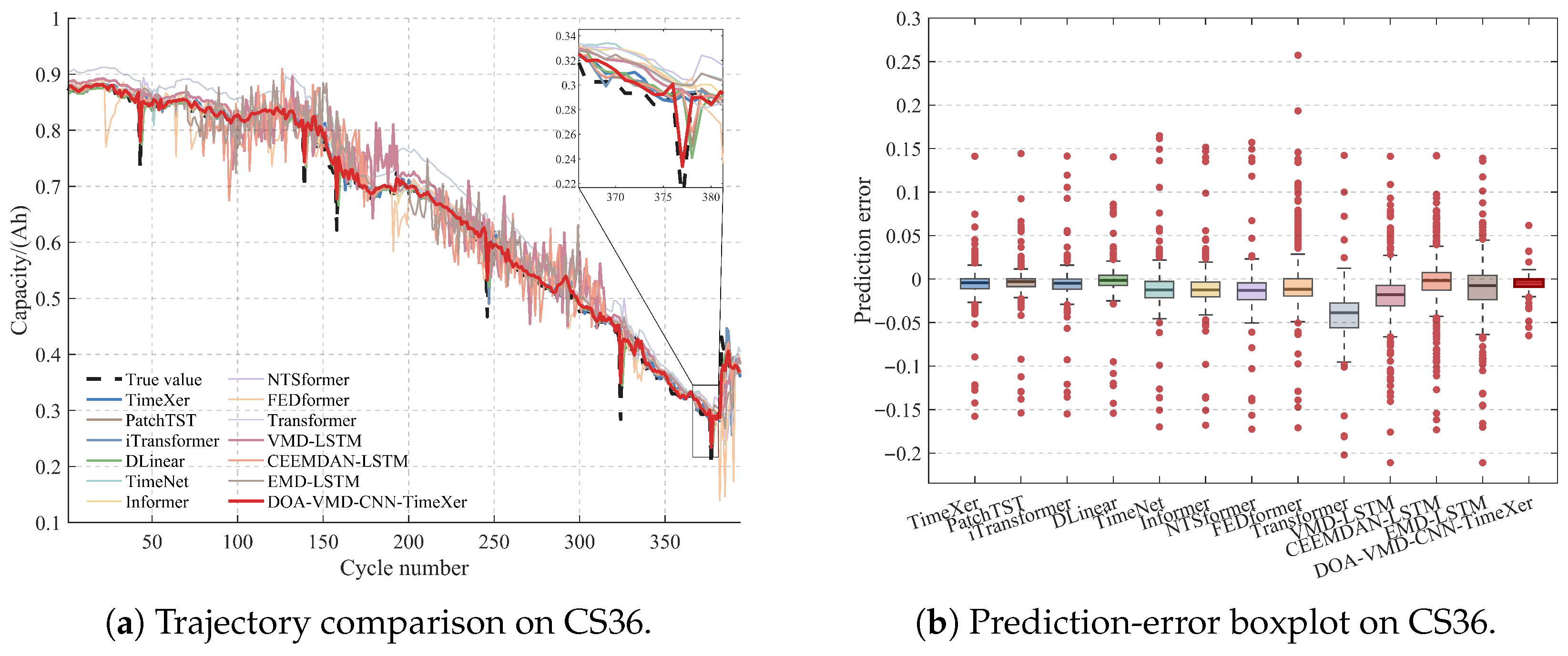
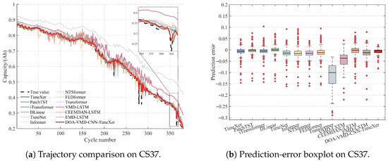
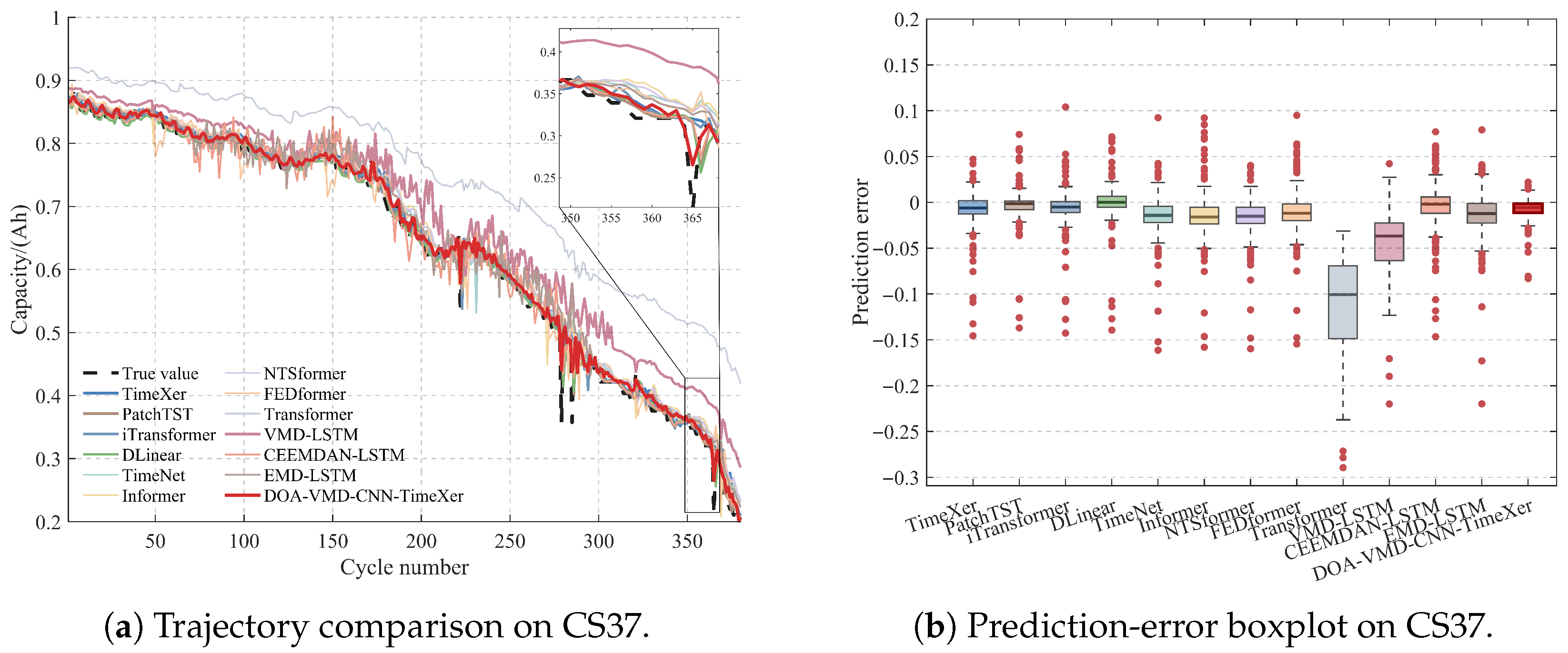
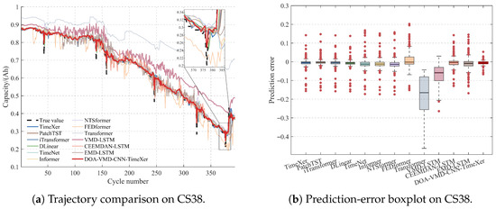
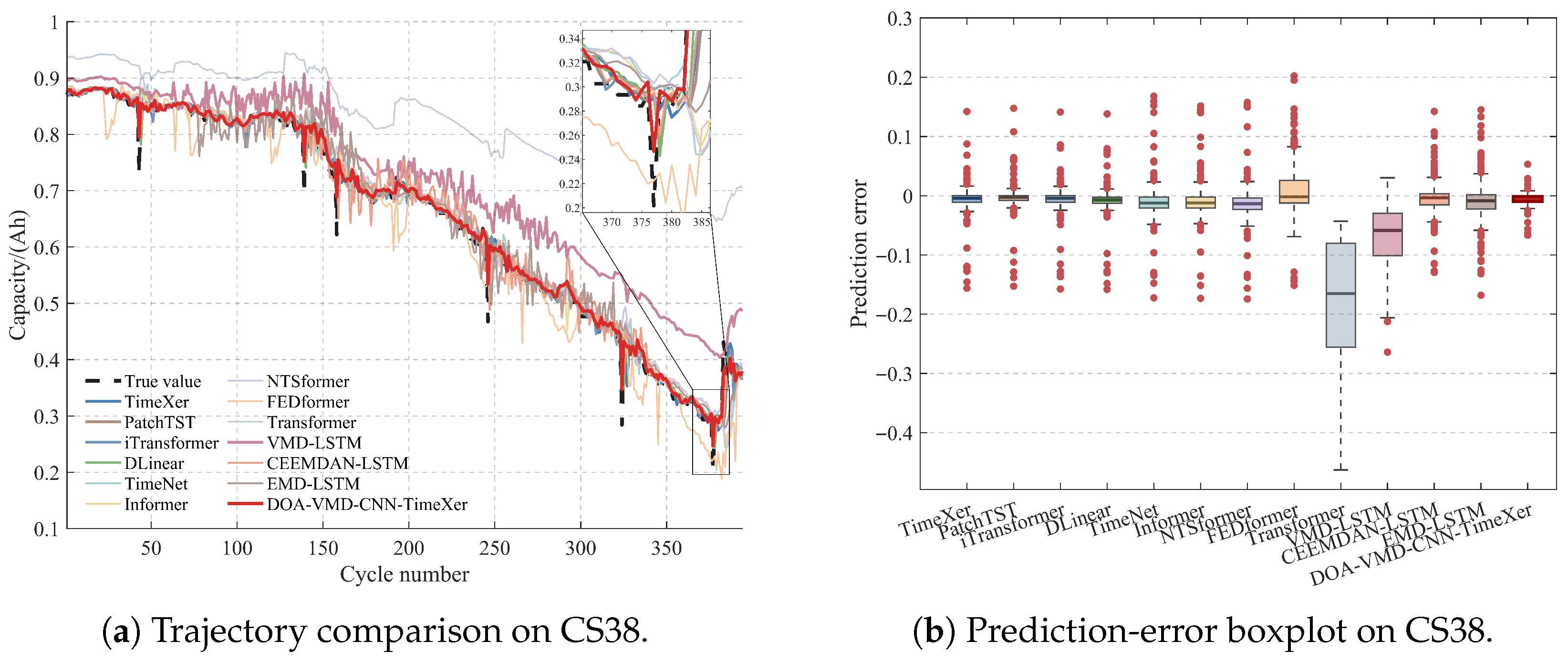
To complement the aggregate metrics in Table 9, Figure 10, Figure 11, Figure 12 and Figure 13 present paired visual comparisons for the 6:4 split, where each figure contains a trajectory-level comparison of all competing methods, together with the corresponding prediction-error boxplot for one cell. These paired visualizations provide two complementary perspectives: the left panel reveals whether a model can follow the overall degradation trend and local fluctuations, whereas the right panel shows whether the resulting errors are concentrated around zero with limited dispersion. Across all four cells, DOA-VMD-CNN-TimeXer remains among the closest trajectories to the measured capacity curve and exhibits compact error distributions centered near zero, which is consistent with its superior RMSE and R² values in Table 9.

Figure 10. Paired model-comparison visualizations for CS35. Panel (a) shows that the proposed DOA-VMD-CNN-TimeXer method remains close to the measured trajectory during both gradual fading and the later fluctuating region. Panel (b) summarizes the corresponding prediction-error distributions and shows that the errors remain concentrated near zero.

Figure 11. Paired model-comparison visualizations for CS36. Panel (a) highlights that the proposed DOA-VMD-CNN-TimeXer method remains better aligned with the measured trajectory across the mid-stage degradation region and the later abrupt drops than the weaker baselines. Panel (b) summarizes the corresponding prediction-error distributions.

Figure 12. Paired model-comparison visualizations for CS37. Panel (a) shows that the proposed DOA-VMD-CNN-TimeXer method preserves close agreement with the measured monotonic degradation path while still responding to local disturbances. Panel (b) summarizes the corresponding prediction-error distributions.

Figure 13. Paired model-comparison visualizations for CS38. Panel (a) shows that the proposed DOA-VMD-CNN-TimeXer method remains better aligned with the measured trajectory during late-stage abrupt drops and subsequent fluctuations. Panel (b) summarizes the corresponding prediction-error distributions.

The cell-wise plots further clarify how the advantage manifests under the 6:4 split. Across all four cells, the proposed method remains among the closest trajectories to the measured curves and keeps a tighter error concentration around zero than the weaker baselines; Figure 11 is representative in showing both improved alignment through the mid-stage decline and abrupt capacity drops and a more compact error distribution. This visual evidence supports the conclusion that the proposed framework improves both trajectory fidelity and error stability under the 6:4 split.

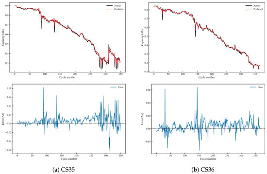
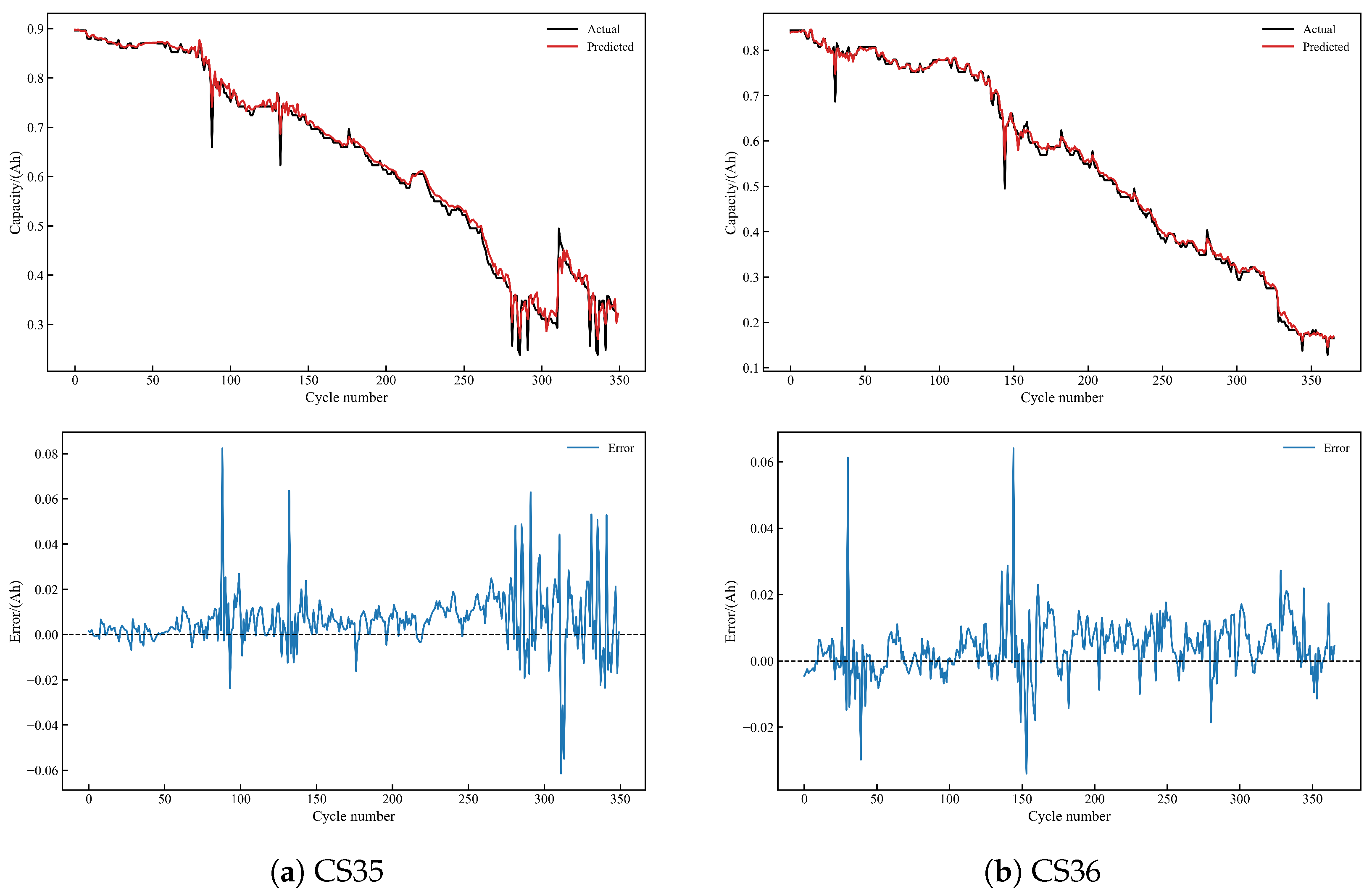
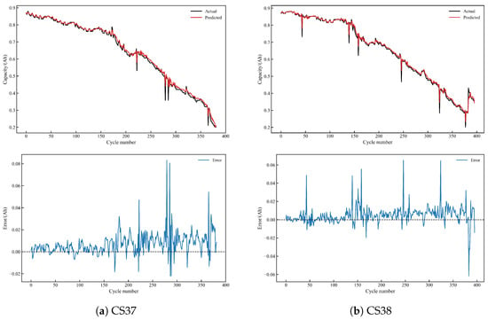
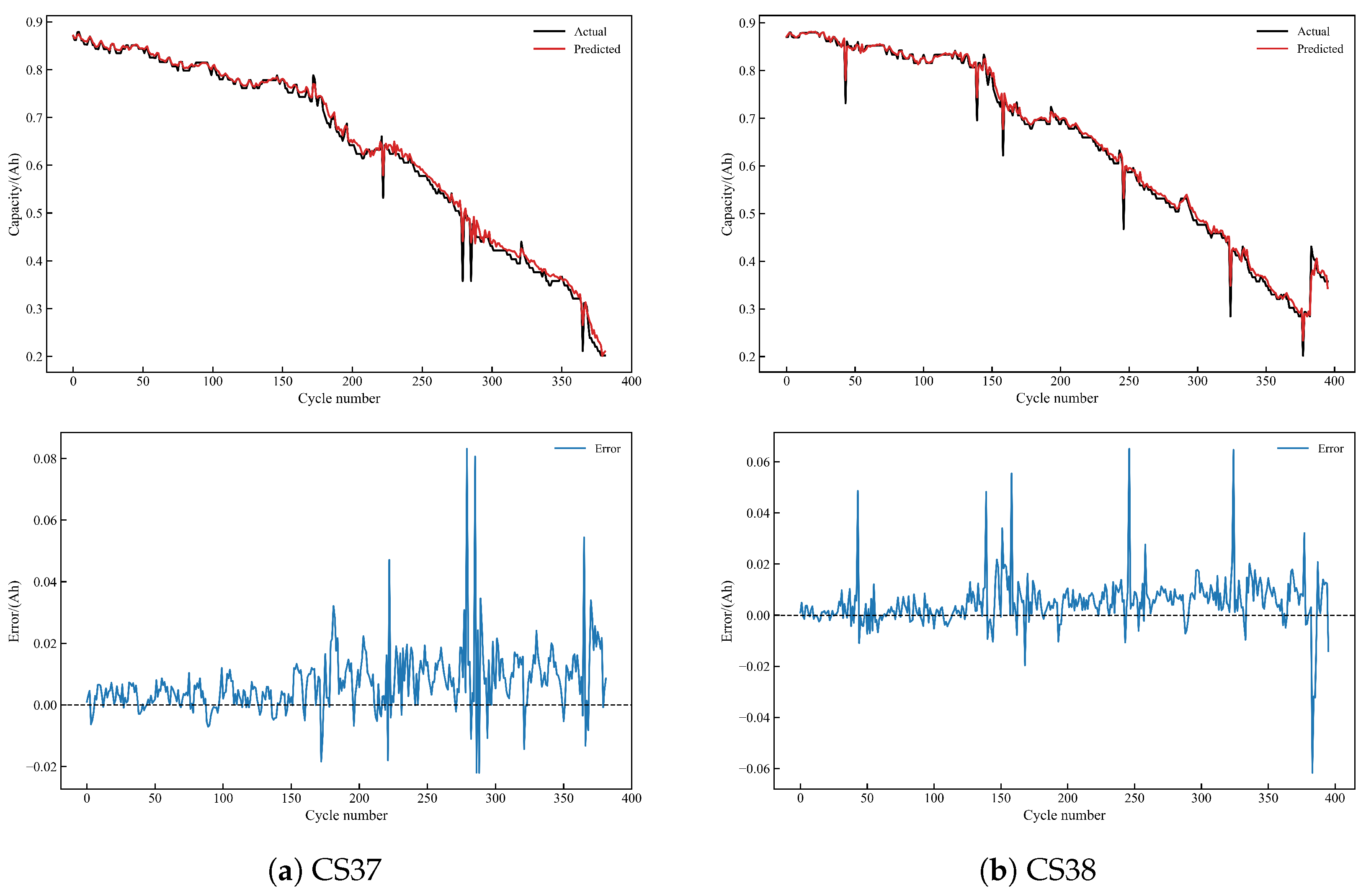
For completeness, Figure 14a,b and Figure 15a,b further isolate the trajectory-level prediction and residual behavior of the proposed model under the primary 5:5 split. Across all four cells, the predicted curves remain closely aligned with the measured capacity evolution over most cycles, and the residual series fluctuate around zero without an obvious persistent offset, indicating limited systematic bias. The proposed method also preserves this alignment around local regeneration-like perturbations and abrupt capacity drops, suggesting reliable trajectory-following ability across the four tested cells.

Figure 14. Trajectory fitting and prediction-error profiles of the proposed DOA-VMD-CNN-TimeXer model on CS35 and CS36 under the 5:5 split. Each subfigure contains the actual-versus-predicted capacity curve (top) and the corresponding prediction-error sequence (bottom).

Figure 15. Trajectory fitting and prediction-error profiles of the proposed DOA-VMD-CNN-TimeXer model on CS37 and CS38 under the 5:5 split. Each subfigure contains the actual-versus-predicted capacity curve (top) and the corresponding prediction-error sequence (bottom).

Overall, the improved performance of DOA-VMD-CNN-TimeXer under the evaluated settings should be understood as the result of module synergy rather than model capacity alone. The DOA-VMD stage decomposes the raw non-stationary sequence into modal components with clearer temporal structure, the CNN branch strengthens the extraction of local fluctuation cues within each component, and the TimeXer branch models long-range cross-cycle evolution after decomposition. The joint effect of these three stages is reflected in both the lower tabulated errors and the more compact, less biased residual behavior observed in Figure 14a,b and Figure 15a,b.

5. Conclusions

This study proposed a DOA-VMD-CNN-TimeXer framework for lithium-ion battery RUL-oriented prognosis through capacity trajectory prediction and reconstruction. The framework combines adaptive VMD parameter optimization, CNN-based local feature extraction, and TimeXer-based long-range temporal modeling, thereby forming a coordinated modeling chain for non-stationary battery degradation sequences.

Experiments on four CALCE lithium-ion battery cells demonstrate that the proposed framework delivers the best overall trajectory-prediction performance among the compared methods under the evaluated settings. Under the primary 5:5 split, the RMSE values are 0.011650, 0.012158, 0.010316, and 0.011343 for CS35–CS38, respectively, and under the supplementary 6:4 split they remain at 0.014528, 0.010887, 0.012506, and 0.011394, with all corresponding R² values above 0.994. Together, the decomposition analysis, ablation study, comparative results, and trajectory-level residual behavior indicate that the performance gain arises from the synergy of adaptive decomposition, local fluctuation extraction, and long-range temporal modeling rather than from any single module in isolation.

From a practical perspective, the proposed method should be regarded as an RUL-oriented capacity trajectory modeling framework rather than as a direct end-to-end RUL regressor. Its value lies in improving the fidelity and stability of reconstructed degradation trajectories, thereby providing a more reliable basis for threshold-based end-of-life and RUL estimation. In this sense, the proposed framework realizes RUL prediction through capacity trajectory forecasting and subsequent threshold-based end-of-life inference, which is consistent with a trajectory-based paradigm widely used in data-driven battery prognostics.

In practical battery management applications, the proposed DOA-VMD-CNN-TimeXer framework is more suitable as an auxiliary prognosis module than as a stand-alone replacement for existing battery management systems. A feasible usage pattern is to perform offline training with historical degradation data collected under representative operating conditions and then deploy the trained model for online capacity trajectory updating as new cycle data become available. In this way, the predicted degradation trajectory can support threshold-based end-of-life determination, remaining useful life estimation, abnormal-degradation warning, maintenance scheduling, and retirement or second-life screening decisions.

Several limitations should also be acknowledged. The current validation is restricted to four CALCE cells from a limited dataset, and the evaluation emphasizes capacity trajectory prediction metrics rather than explicit RUL-threshold error indices. Transfer-learning-based battery health modeling and degradation knowledge transfer are also complementary directions to the present capacity trajectory forecasting framework, suggesting that future work should further investigate cross-chemistry generalization and transfer-aware degradation prognosis on larger and more heterogeneous battery datasets. Joint optimization of decomposition parameters and CNN-TimeXer hyper-parameters also remains a relevant direction for future work, although such a search would substantially increase the total training cost. Future work will therefore focus on extending the framework to larger and more heterogeneous battery datasets, incorporating direct RUL-oriented evaluation criteria, investigating robustness under variable operating conditions and uncertainty-aware prognosis settings, and exploring optimization-based hyper-parameter tuning for the predictor.

References

- Ma, G.; Zhang, Y.; Cheng, C.; Zhou, B.; Hu, P.; Yuan, Y. Remaining Useful Life Prediction of Lithium-Ion Batteries Based on False Nearest Neighbors and a Hybrid Neural Network. Appl. Energy 2019, 253, 113626. [Google Scholar] [CrossRef] [Scilit]
- Hu, X.; Xu, L.; Lin, X.; Pecht, M. Battery Lifetime Prognostics. Joule 2020, 4, 310–346. [Google Scholar] [CrossRef] [Scilit]
- Han, X.; Lu, L.; Zheng, Y.; Feng, X.; Li, Z.; Li, J.; Ouyang, M. A Review on the Key Issues of the Lithium Ion Battery Degradation among the Whole Life Cycle. eTransportation 2019, 1, 100005. [Google Scholar] [CrossRef] [Scilit]
- Wang, Z.; Liu, N.; Chen, C.; Guo, Y. Adaptive Self-Attention LSTM for RUL Prediction of Lithium-Ion Batteries. Inf. Sci. 2023, 635, 398–413. [Google Scholar] [CrossRef] [Scilit]
- Hasib, S.A.; Islam, S.; Chakrabortty, R.K.; Ryan, M.J.; Saha, D.K.; Ahamed, M.H.; Moyeen, S.I.; Das, S.K.; Ali, M.F.; Islam, M.R.; et al. A Comprehensive Review of Available Battery Datasets, RUL Prediction Approaches, and Advanced Battery Management. IEEE Access 2021, 9, 86166–86193. [Google Scholar] [CrossRef] [Scilit]
- Meng, J.; Luo, G.; Ricco, M.; Swierczynski, M.; Stroe, D.I.; Teodorescu, R. Overview of Lithium-Ion Battery Modeling Methods for State-of-Charge Estimation in Electrical Vehicles. Appl. Sci. 2018, 8, 659. [Google Scholar] [CrossRef] [Scilit]
- Yang, F.; Xing, Y.; Wang, D.; Tsui, K.L. A Comparative Study of Three Model-Based Algorithms for Estimating State-of-Charge of Lithium-Ion Batteries under a New Combined Dynamic Loading Profile. Appl. Energy 2016, 164, 387–399. [Google Scholar] [CrossRef] [Scilit]
- Wang, Y.; Chen, Z. A Framework for State-of-Charge and Remaining Discharge Time Prediction Using Unscented Particle Filter. Appl. Energy 2020, 260, 114324. [Google Scholar] [CrossRef] [Scilit]
- Li, Y.; Su, B.; Duan, B. State-of-Charge Estimation Tolerant of Battery Aging Based on a Physics-Based Model and an Adaptive Cubature Kalman Filter. Energy 2021, 220, 119767. [Google Scholar] [CrossRef] [Scilit]
- Li, X.; Yuan, C.; Wang, Z. State of Health Estimation for Li-Ion Battery via Partial Incremental Capacity Analysis Based on Support Vector Regression. Energy 2020, 203, 117852. [Google Scholar] [CrossRef] [Scilit]
- Wu, W.; Lu, S. Remaining Useful Life Prediction of Lithium-Ion Batteries Based on Data Preprocessing and Improved ELM. IEEE Trans. Instrum. Meas. 2023, 72, 1–14. [Google Scholar] [CrossRef] [Scilit]
- Liu, D.; Zhou, J.; Pan, D.; Peng, Y.; Peng, X. Lithium-Ion Battery Remaining Useful Life Estimation with an Optimized Relevance Vector Machine Algorithm with Incremental Learning. Measurement 2015, 63, 143–151. [Google Scholar] [CrossRef] [Scilit]
- Guo, W.; He, M. An Optimal Relevance Vector Machine with a Modified Degradation Model for Remaining Useful Lifetime Prediction of Lithium-Ion Batteries. Appl. Soft Comput. 2022, 124, 108967. [Google Scholar] [CrossRef] [Scilit]
- Zhou, Y.; Huang, M. Lithium-Ion Batteries Remaining Useful Life Prediction Based on a Mixture of Empirical Mode Decomposition and ARIMA Model. Microelectron. Reliab. 2016, 65, 265–273. [Google Scholar] [CrossRef] [Scilit]
- Li, X.; Zhang, L.; Wang, Z.; Dong, P. Remaining Useful Life Prediction for Lithium-Ion Batteries Based on a Hybrid Model Combining the Long Short-Term Memory and Elman Neural Networks. J. Energy Storage 2019, 21, 510–518. [Google Scholar] [CrossRef] [Scilit]
- Wang, J.; Xiang, Y. Fast Modeling of the Capacity Degradation of Lithium-Ion Batteries via a Conditional Temporal Convolutional Encoder–Decoder. IEEE Trans. Transp. Electrif. 2022, 8, 1695–1709. [Google Scholar] [CrossRef] [Scilit]
- Liu, K.; Shang, Y.; Ouyang, Q.; Widanage, W.D. A Data-Driven Approach with Uncertainty Quantification for Predicting Future Capacities and Remaining Useful Life of Lithium-Ion Battery. IEEE Trans. Ind. Electron. 2021, 68, 3170–3180. [Google Scholar] [CrossRef] [Scilit]
- Ding, G.; Wang, W.; Zhu, T. Remaining Useful Life Prediction for Lithium-Ion Batteries Based on CS-VMD and GRU. IEEE Access 2022, 10, 89402–89413. [Google Scholar] [CrossRef] [Scilit]
- Ouyang, Z.; Shen, Y. Prediction of Remaining Useful Life of Lithium Batteries Based on WOA-VMD and LSTM. Energies 2022, 15, 8918. [Google Scholar] [CrossRef] [Scilit]
- Zhu, H.; Dong, G.; Wang, K.; Li, X.; Pedrycz, W. Prognosis of Lithium-Ion Batteries’ Remaining Useful Life Based on a Sequence-to-Sequence Model with Variational Mode Decomposition. Energies 2023, 16, 803. [Google Scholar] [CrossRef] [Scilit]
- Shi, Z.; Guo, C.; Chen, X.; Lu, X.; Le, B.; Liu, H. Successive Variational Mode Decomposition and Optimized Long Short-Term Memory Networks for Predicting the Remaining Useful Life of Lithium-Ion Batteries. Energies 2023, 16, 5952. [Google Scholar] [CrossRef] [Scilit]
- Wang, S.; Ma, H.; Zhang, Y.; Li, S.; He, W. Research on the Remaining Useful Life Prediction Method of Lithium-Ion Batteries Based on Variational Modal Decomposition and Deep Learning Integrated Approach. Energy 2023, 282, 128984. [Google Scholar] [CrossRef] [Scilit]
- Wei, M.; Ye, M.; Zhang, C.; Li, Y.; Zhang, J.; Wang, Q. A Multi-Scale Learning Approach for Remaining Useful Life Prediction of Lithium-Ion Batteries Based on Variational Mode Decomposition and Monte Carlo Sampling. Energy 2023, 278, 129086. [Google Scholar] [CrossRef] [Scilit]
- Yuan, Z.; Tian, T.; Hao, F.; Li, G.; Wu, B.; Lian, C. A Hybrid Neural Network Based on Variational Mode Decomposition Denoising for Predicting State-of-Health of Lithium-Ion Batteries. J. Power Sources 2024, 620, 234697. [Google Scholar] [CrossRef] [Scilit]
- Gu, X.; See, K.Y.; Li, S.; Shan, M.; Wang, C.; Zhao, Y.; Lim, T.H.; Zhang, Y. A Novel State-of-Health Estimation for the Lithium-Ion Battery Using a Convolutional Neural Network and Transformer Model. Energy 2023, 263, 125501. [Google Scholar] [CrossRef] [Scilit]
- Jia, C.; Tian, Y.; Shi, Y.; Jia, J.; Wen, J.; Zeng, J. State of Health Prediction of Lithium-Ion Batteries Based on Bidirectional Gated Recurrent Unit and Transformer. Energy 2023, 285, 129401. [Google Scholar] [CrossRef] [Scilit]
- Quan, R.; Zhou, Y.; Li, W.; Wan, H. A Hybrid Data-Driven Approach for SOH Estimation of Lithium-Ion Batteries Based on Health Index Extraction and QHDBO-BiTCN-BiGRU. J. Energy Storage 2025, 125, 116788. [Google Scholar] [CrossRef] [Scilit]
- Zheng, J.; Ma, L.; Lei, C.; Zhang, Z.; Chen, X.; Xie, Y. Refined Lithium-Ion Battery State of Health Estimation with Charging Segment Adjustment. Appl. Energy 2024, 372, 124077. [Google Scholar] [CrossRef] [Scilit]
- Zhu, J.; Ma, J.; Wu, J. A Regularized Constrained Two-Stream Convolution Augmented Transformer for Aircraft Engine Remaining Useful Life Prediction. Eng. Appl. Artif. Intell. 2024, 133, 108161. [Google Scholar] [CrossRef] [Scilit]
- Sun, J.; Li, S.; Ge, W.; Zheng, S. Remaining Useful Life Prognostics of Bearings Based on Convolution Attention Networks and Enhanced Transformer. Heliyon 2024, 10, e38317. [Google Scholar] [CrossRef] [Scilit] [PubMed]
- Wang, F.; Zhai, Z.; Zhao, Z.; Di, Y.; Chen, X. Physics-Informed Neural Network for Lithium-Ion Battery Degradation Stable Modeling and Prognosis. Nat. Commun. 2024, 15, 4332. [Google Scholar] [CrossRef] [Scilit]
- Hao, S.; Feng, J.; Dong, J.; Cui, W.; Cheng, J.; Gong, M. Physics-Informed Hierarchical Perception Modulation Network for Lithium-Ion Battery Health Management. Energy 2025, 335, 138229. [Google Scholar] [CrossRef] [Scilit]
- Wang, Z.; Liu, Y.; Wang, F.; Wang, H.; Su, M. Capacity and Remaining Useful Life Prediction for Lithium-Ion Batteries Based on Sequence Decomposition and a Deep-Learning Network. J. Energy Storage 2023, 72, 108085. [Google Scholar] [CrossRef] [Scilit]
- Zhao, B.; Zhang, W.; Zhang, Y.; Zhang, C.; Zhang, C.; Zhang, J. Research on the Remaining Useful Life Prediction Method for Lithium-Ion Batteries by Fusion of Feature Engineering and Deep Learning. Appl. Energy 2024, 358, 122325. [Google Scholar] [CrossRef] [Scilit]
- Lang, Y.; Gao, Y. Dream Optimization Algorithm (DOA): A Novel Metaheuristic Optimization Algorithm Inspired by Human Dreams and Its Applications to Real-World Engineering Problems. Comput. Methods Appl. Mech. Eng. 2025, 436, 117718. [Google Scholar] [CrossRef] [Scilit]
- Dragomiretskiy, K.; Zosso, D. Variational Mode Decomposition. IEEE Trans. Signal Process. 2014, 62, 531–544. [Google Scholar] [CrossRef] [Scilit]
- Zhang, Y.; Zhang, T.; Tian, L. A TimeXer-Based Numerical Forecast Correction Model Optimized by an Exogenous-Variable Attention Mechanism. Comput. Mater. Contin. 2026, 86, 76. [Google Scholar] [CrossRef] [Scilit]
- Li, Z.; Yan, B.; Meng, Q.; Xu, C.; Zhang, F.; Wang, Y.; Domingo, M. Strain Prediction in a Large-Span Arch Bridge Using the TimeXer Model Considering Temperature and Traffic Loads. Front. Built Environ. 2026, 12, 1749222. [Google Scholar] [CrossRef] [Scilit]
Disclaimer/Publisher’s Note: The statements, opinions and data contained in all publications are solely those of the individual author(s) and contributor(s) and not of MDPI and/or the editor(s). MDPI and/or the editor(s) disclaim responsibility for any injury to people or property resulting from any ideas, methods, instructions or products referred to in the content. |
© 2026 by the authors. Licensee MDPI, Basel, Switzerland. This article is an open access article distributed under the terms and conditions of the Creative Commons Attribution (CC BY) license.