Identification of Distribution-Network Edge-End Devices Based on Current Time–Frequency Features and Random Forest

Abstract

With the increasing integration of distributed photovoltaics, energy storage systems, electric vehicle chargers, and intelligent terminals, accurate identification of heterogeneous edge-end devices in distribution networks has become challenging due to their diverse operating characteristics and similar current signatures. This paper proposes an identification method based on current time–frequency features and Random Forest. Equivalent grid-connected current models are developed for five types of edge-end devices, considering different capacity levels, operating states, ripple characteristics, and transient behaviors. A 13-dimensional feature set is extracted from time-domain, frequency-domain, and time–frequency characteristics, covering 11 device subclasses. Feature analysis is conducted to evaluate the separability of the extracted features, and Random Forest is employed for multi-class device identification. The results show that the proposed method achieves an overall accuracy above 98% on independent test samples and 96.91% in the IEEE 33-bus validation case, demonstrating its effectiveness for distribution-network edge-end device identification.

1. Introduction

With the increasing integration of distributed photovoltaics, energy storage systems, electric vehicle charging facilities, and intelligent terminals, distribution networks are evolving toward multi-source access and bidirectional interactions. New-type distribution-network construction, cyber-physical data fusion modeling, and panoramic information perception have become important for improving operational awareness [1,2,3]. Consequently, current signals at feeder ends and transformer districts contain not only conventional load information but also device-dependent characteristics associated with power-electronic conversion, charge/discharge control, switching behaviors, and terminal power consumption. Accurate identification of heterogeneous edge-end devices remains challenging due to variations in capacity, operating states, harmonic characteristics, and background disturbances.

Edge-end device identification is closely related to non-intrusive load monitoring (NILM). Existing studies have explored event-based features, temporal features, V-I trajectories, deep learning, and ensemble learning methods [4,5,6,7,8]. However, distribution-network edge devices are commonly connected through power-electronic interfaces, leading to overlapping harmonic and ripple characteristics among different device types. Therefore, identification performance can be limited when relying on a single feature representation. Moreover, practical deployment requires not only high accuracy but also interpretable features, moderate computational cost, and consistent data-processing procedures.

Random Forest is suitable for classification problems involving structured features and nonlinear boundaries. It constructs multiple decision trees through bootstrap sampling and random feature selection and determines class labels through majority voting [9,10,11,12]. Previous studies have demonstrated its effectiveness in nonlinear and noisy identification tasks [13,14]. Based on this consideration, this paper proposes a distribution-network edge-end device identification method using current time–frequency features and Random Forest. Different from conventional NILM studies focusing on household appliances or aggregated loads, this work targets heterogeneous distribution-network edge devices and develops device-oriented current features considering magnitude, harmonic distortion, switching-related components, and short-term fluctuations.

Based on these considerations, this paper proposes a distribution-network edge-end device identification method based on current time–frequency features and Random Forest. The proposed framework consists of equivalent current modeling, feature extraction, classifier construction, and scenario validation. Different from conventional NILM studies that mainly focus on household appliances or aggregated loads, this work targets heterogeneous edge-end devices in distribution networks, whose current characteristics are affected by device structures, control strategies, and operating states. A device-oriented feature representation is developed by considering current magnitude, waveform distortion, harmonic characteristics, switching-related components, and short-term fluctuations. The proposed method is validated using independent test samples and an IEEE 33-bus distribution-network scenario.

The main contributions are as follows: (1) equivalent grid-connected current models are established for five typical classes of edge-end devices, yielding 11 identification labels; (2) a 13-dimensional current feature system covering time-domain, frequency-domain, and time–frequency fluctuation information is constructed, and its separability is analyzed by statistical distribution, correlation analysis, and dimensionality reduction; and (3) a Random-Forest-based identification workflow is established and validated through multi-algorithm comparison and IEEE 33-bus case studies.

2. Current Modeling and Feature-System Construction for Edge-End Devices

2.1. Identification Targets and Modeling Assumptions

Five common edge-end devices with significant electrical differences in distribution networks are selected as the study objects: distributed photovoltaics (PV), distributed energy storage systems (ES), electric vehicle charging piles (EV), smart circuit breakers (IB), and intelligent fusion terminals (IF). Among them, PV, ES, and EV are further divided into three subclasses according to capacity level or rated power, whereas IB and IF are represented by a single typical model. As a result, the identification task contains 11 subclasses. This classification preserves inter-class differences while also reflecting the intra-class variation caused by capacity level or power rating.

To generate samples in batches and support subsequent feature analysis, equivalent grid-connected current models are established under the assumptions of three-phase symmetrical operation, single-phase equivalent modeling, and steady-state observation within short time windows. The models do not attempt to fully reproduce the internal details of controllers, filters, or switching devices; instead, they retain the components most relevant to identification, including magnitude scale, low-order harmonics, high-frequency ripple, short-term fluctuations, and random noise. This treatment reduces simulation complexity and facilitates the construction of a unified feature database.

$$I_k={\displaystyle \frac{P_k}{\sqrt{3}{U}_k}}$$

(1)

Equation (1) gives the approximate calculation of the rated line current for the k-th device capacity grade, where Pk denotes the rated capacity or rated power and Uk denotes the access voltage level. For energy storage devices, the rated power can be estimated from the energy capacity and the C-rate; for charging piles, the rated power is determined by the slow-, fast-, and ultra-fast-charging categories. On this basis, the single-phase grid-connected currents of all device types can be expressed in the following unified form:

$$i(t)=i_1(t)+{\displaystyle \sum _{\mathrm{h}}{i}_h}(t)+i_{hf}(t)+i_{fluct}(t)+n(t)$$

(2)

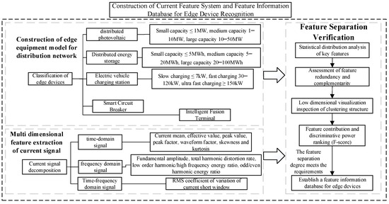
where $i_1(t)$ is the power-frequency fundamental component, $i_{\mathrm{h}}(t)$ is the low-order harmonic component, $i_{\mathrm{hf}}(t)$ is the high-frequency switching-ripple component, $i_{\mathrm{fluct}}(t)$ denotes disturbances such as irradiance variation, charging/discharging ramps, charging-stage transitions, or short-duration surge currents, and $n(t)$ is random noise. The differences among device types in harmonic order, ripple band, disturbance pattern, and magnitude level constitute the physical basis for subsequent feature extraction and classification. The overall framework for constructing the current-feature system is shown in Figure 1. The main components and modeling characteristics of the five device types are summarized in Table 1.

Figure 1. Framework for constructing the current-feature system for edge-end device identification.

Table 1. Elements of the grid-connected current models for five types of edge-end devices.

Device Type	Internal Classification	Main Current Components	Modeling Focus
PV	Small/Medium/Large Capacity	Fundamental, 3rd/5th/7th harmonics, 2–3 kHz ripple, random noise	Irradiance envelope, inverter switching ripple, and capacity-level differences
ES	Small/Medium/Large Capacity	Fundamental, 5th/7th/11th harmonics, 1.5–3 kHz ripple, random noise	Charge/discharge direction, power settings, and slow-varying ramps
EV	Slow/Fast/Ultra-Fast Charging	Fundamental, 3rd/5th/7th harmonics, 2–4 kHz and 6–10 kHz ripple bands, random noise	Power level, rectifier harmonics, and CC-CV stage variation
IB	Single Typical Model	Fundamental, 3rd/5th harmonics, short-duration surge current, random noise	Low-amplitude load current and switching-surge events
IF	Single Typical Model	Fundamental, 2nd/3rd harmonics, 5–6 kHz and 8–9 kHz ripple bands, random noise	Terminal self-consumption, even-order harmonics, and switch-mode-power-supply ripple

2.2. Physical Mechanisms of Current Features for Different Device Types

The AC-side current characteristics of distributed photovoltaics are mainly determined by inverter grid-connected control. Within a short observation window, irradiance variation appears as a slow envelope, while inverter switching introduces high-frequency ripple in specific frequency bands. PV units with different capacity levels exhibit different current magnitudes, access conditions, and relative harmonic/ripple components due to variations in device capacity and filtering characteristics. Therefore, features such as RMS, fundamental amplitude, THD, and HF_ratio can reflect both capacity-related information and power-electronic characteristics. In sample generation, the slow envelope modulation frequency of PV is set to 0.2–0.5 Hz, with an amplitude variation of 5–15% of the rated current. The load factor is randomly selected between 30% and 100% to represent different irradiance conditions while remaining constant within each observation window.

Distributed energy storage systems are connected to distribution networks through bidirectional converters and can operate in both charging and discharging modes. The power direction affects the current phase, while dispatch commands introduce slow amplitude variations. Their harmonic characteristics are mainly associated with converter control and filtering conditions, where the fifth-, seventh-, and 11th-order harmonics and high-frequency ripple provide representative signatures. Compared with PV units, ES devices exhibit stronger controllability, resulting in larger intra-class variations under different charging/discharging states. Therefore, a linear ramp with a total variation of ±5% of rated power is applied within the 0.2 s window to represent gradual power adjustment. The power setpoint is randomly selected between 30% and 100% of the rated capacity. The extracted features are selected according to the physical characteristics of edge-end devices rather than predefined class labels.

The current characteristics of electric vehicle charging piles are closely related to charging power levels and charging stages. The charging process typically involves constant-current, constant-voltage, or multi-stage control, leading to variations in current magnitude, harmonic distortion, and short-term fluctuations [15,16]. Slow chargers usually exhibit lower current levels, which may overlap with low-voltage loads or smart circuit breakers, increasing identification difficulty. In contrast, fast and ultra-fast chargers show larger current magnitudes, stronger rectifier harmonics, and more obvious high-frequency ripple. Since charging-stage transitions may introduce local fluctuations, RMS_CV (Short-Window RMS Coefficient of Variation) is used to characterize short-term current variations. For EV samples, sinusoidal envelope modulation is applied with amplitudes of 2%, 5%, and 10% for slow, fast, and ultra-fast chargers, respectively. The charging load factor is randomly selected between 60% and 100% to represent different charging states.

The current magnitudes of smart circuit breakers and intelligent fusion terminals are generally lower than those of high-power distributed resources; however, their waveform characteristics still provide identifiable information. The current of smart circuit breakers is close to that of conventional loads, with occasional short-duration surges or switching transients. Intelligent fusion terminals contain power-supply and communication modules, resulting in more noticeable even-order harmonics, high-frequency ripple, and small random disturbances. In this study, the ripple amplitude of intelligent fusion terminals is modeled as approximately 10–20% of the fundamental current amplitude. Although relatively small in magnitude, its spectral distribution provides useful identification information. Therefore, HF_ratio, odd-even harmonic ratio, and peak-related features contribute to distinguishing these two device types.

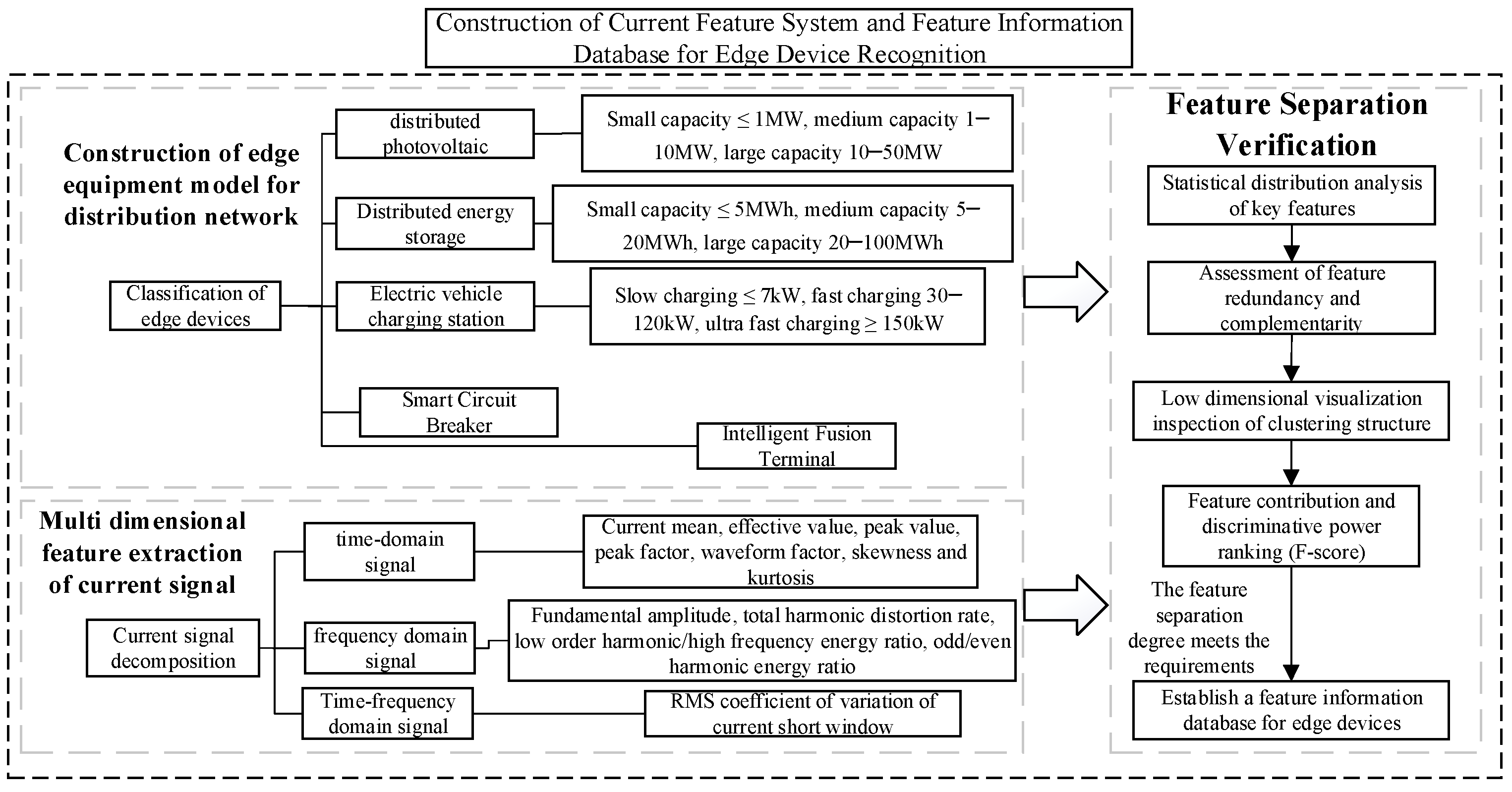
Figure 2 shows the typical grid-connected current waveforms of the five device types. It can be observed that PV, ES, and EV are all dominated by the power-frequency fundamental component, but they differ significantly in magnitude scale and local ripple. The IB waveform is relatively smooth, with occasional surges at some instants, whereas IF exhibits smaller amplitude but more pronounced high-frequency ripple. The raw waveforms alone cannot form a stable classification boundary, so structured features must be further extracted.

Figure 2. Typical grid-connected current waveforms of five types of edge-end devices.

2.3. Definition of the 13-Dimensional Current Features

Each current sample is transformed into a 13-dimensional feature vector, including time-domain statistics, frequency-domain harmonic characteristics, and time-varying fluctuation information. Let the discrete current sequence be i(n), n = 0, 1,…, N − 1, with sampling frequency f_s and observation-window length T. Time-domain features describe current magnitude, waveform sharpness, and statistical distribution, while fluctuation features characterize intra-window variations through the coefficient of variation of short-window RMS.

Frequency-domain features include harmonic distortion, low-order harmonic energy, high-frequency ripple energy, and odd–even harmonic structure. The low-order harmonic energy ratio is calculated from the second–seventh harmonic components of the 50 Hz fundamental, and characteristic harmonic components (third, fifth, seventh, and 11th orders) are used to describe nonlinear conversion behaviors. Switching-related components are separately extracted as high-frequency ripple features based on device-dependent kHz bands (1.5–3 kHz for ES, 2–3 kHz for PV, and 2–4 kHz/6–10 kHz for EV charging piles) and quantified by HF_ratio rather than treated as conventional harmonics.

$$x={\left[I_{mean},I_{rms},I_{peak},\mathrm{CF},\mathrm{FF},\mathrm{Skew},\mathrm{Kurt},I_1,\mathrm{THD},\mathrm{lowH}\_\mathrm{ratio},\mathrm{HF}\_\mathrm{ratio},\mathrm{oddeven}\_\mathrm{ratio},\mathrm{RMS}\_\mathrm{CV}\right]}^{\mathrm{T}}$$

(3)

Among these features, the current RMS Irms reflects the overall magnitude level of a sample, the crest factor CF characterizes waveform sharpness, the form factor FF measures how close the waveform is to a sinusoid, and skewness and kurtosis describe distributional asymmetry and peakedness, respectively. In the frequency domain, each component is obtained by fast Fourier transform. THD is used to quantify total harmonic distortion; the low-order harmonic energy ratio counts the energy of the second to seventh harmonics; the high-frequency energy ratio counts the energy in the 1–5 kHz band; and the odd–even harmonic energy ratio distinguishes the harmonic structures of rectifier-type, switch-mode-power-supply-type, and conventional-load-type devices.

$$\mathrm{THD}={\displaystyle \frac{\sqrt{{\displaystyle \sum _2^H{I}_h^2}}}{I_1}}$$

(4)

$$\mathrm{HF}\_\mathrm{ratio}={\displaystyle \frac{E_{1~5\mathrm{kHz}}}{E_{total}}},\hspace{1em}\hspace{1em}\mathrm{RMS}\_\mathrm{CV}={\displaystyle \frac{std\left(I_{rms,m}\right)}{mean\left(I_{rms,m}\right)}}$$

(5)

where $I_H$ is the amplitude of the h-th harmonic, $I_1$ is the fundamental amplitude, E_1–5kHz is the energy in the high-frequency band, Etotal is the total energy, and I_rms,m is the current RMS within the m-th short window. Compared with using raw sampling points directly, the 13-dimensional feature vector greatly compresses the input dimension while retaining the key information on magnitude, harmonics, and fluctuations that is essential for identification. The mathematical definitions of the 13 features are summarized in Table 2. The overall feature-extraction procedure is illustrated in Figure 3.

Table 2. The 13 current features and their mathematical definitions.

Category	Feature	Symbol	Definition
Time	Current Mean	Imean	$I_{mean}={\displaystyle \frac{1}{N}}{\displaystyle \sum _{n=0}^{N-1}i}[n]$
Time	Current RMS	Irms	$I_{rms}=\sqrt{{\displaystyle \frac{1}{N}}{\displaystyle \sum _{n=0}^{N-1}{i}^2}[n]}$
Time	Current Peak	Ipeak	$I_{peak}={\max }_{0\le n\le N-1}\left|i[n]\right|$
Time	Crest Factor	CF	$\mathrm{CF}=I_{peak}/I_{rms}$
Time	Form Factor	FF	$\mathrm{FF}=I_{rms}/I_{abs}$
Time	Skewness	Skewness	$\mathrm{Skew}={\displaystyle \frac{\frac{1}{N}{\displaystyle \sum _{n=0}^{N-1}{\left(i[n]-I_{mean}\right)}^3}}{{\sigma }^3}}$
Time	Kurtosis	Kurtosis	$\mathrm{Kurt}={\displaystyle \frac{\frac{1}{N}{\displaystyle \sum _{n=0}^{N-1}{\left(i[n]-I_{mean}\right)}^4}}{{\sigma }^4}}$
Frequency	Fundamental Amplitude	I1	$I_1=|I[k_1]|,\hspace{1em}{k}_1=\arg {\min }_k\left|f_k-f_1\right|$
Frequency	THD	THD	$\mathrm{THD}={\displaystyle \frac{\sqrt{{\displaystyle \sum _{h=2}^H{I}_h^2}}}{I_1}}$
Frequency	Low-Order Harmonic Energy Ratio	lowF_ratio	$\mathrm{lowH}\_\mathrm{ratio}={\displaystyle \frac{{\displaystyle \sum _{h=2}^7|}I[k_h]{|}^2}{E_{total}}}$
Frequency	High-Frequency Energy Ratio	HF_ratio	$\mathrm{HF}\_\mathrm{ratio}={\displaystyle \frac{{\displaystyle \sum _{k\in {\mathsf{\Omega }}_{\mathrm{HF}}}|}I[k]{|}^2}{E_{total}}}$
Frequency	Odd–Even Harmonic Energy Ratio	$\mathrm{oddeven}$_ratio	$\mathrm{oddeven}\_\mathrm{ratio}={\displaystyle \frac{E_{odd}}{E_{even}}}$
Time–Frequency	Short-Window RMS Coefficient of Variation	RMS_CV	$\mathrm{RMS}\_\mathrm{CV}={\displaystyle \frac{{\sigma }_R}{{\mu }_R}}$

Figure 3. Multi-dimensional feature-extraction procedure for current signals.

In this study, the supply voltage is assumed to be approximately sinusoidal, and voltage harmonic components are not explicitly considered during feature extraction. Under this assumption, the extracted current features mainly characterize device-dependent behaviors, including harmonic distortion, switching-related ripple, and operating fluctuations. The influence of voltage–current harmonic coupling under highly distorted operating conditions will be further investigated in future work.

2.4. Feature-Database Construction and Data-Processing Workflow

The feature database is constructed under unified simulation and sampling conditions. The sampling frequency is set to fs = 10 kHz, and the observation window is set to T = 0.2 s. Under the 50 Hz fundamental frequency, each sample contains 10 complete cycles and 2000 sampling points. The corresponding FFT frequency resolution is 5 Hz.

The sampling frequency corresponds to a Nyquist frequency of 5 kHz. Therefore, the proposed method extracts spectral features within the measurable bandwidth below 5 kHz, including the fundamental component, low-order harmonics, and switching-related ripple components in the defined frequency bands. The HF_ratio is calculated using FFT bins below 5 kHz, with anti-alias filtering assumed in the acquisition process.

For fluctuation analysis, the 0.2 s window is divided into ten 0.02 s sub-windows, and RMS_CV is calculated from the RMS values of these sub-windows. The selected window length represents a trade-off between feature stability and identification latency under the short-time steady-state conditions considered in this study.

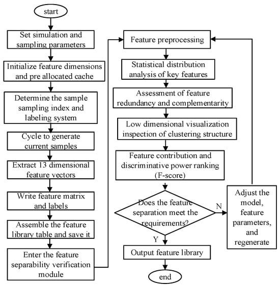
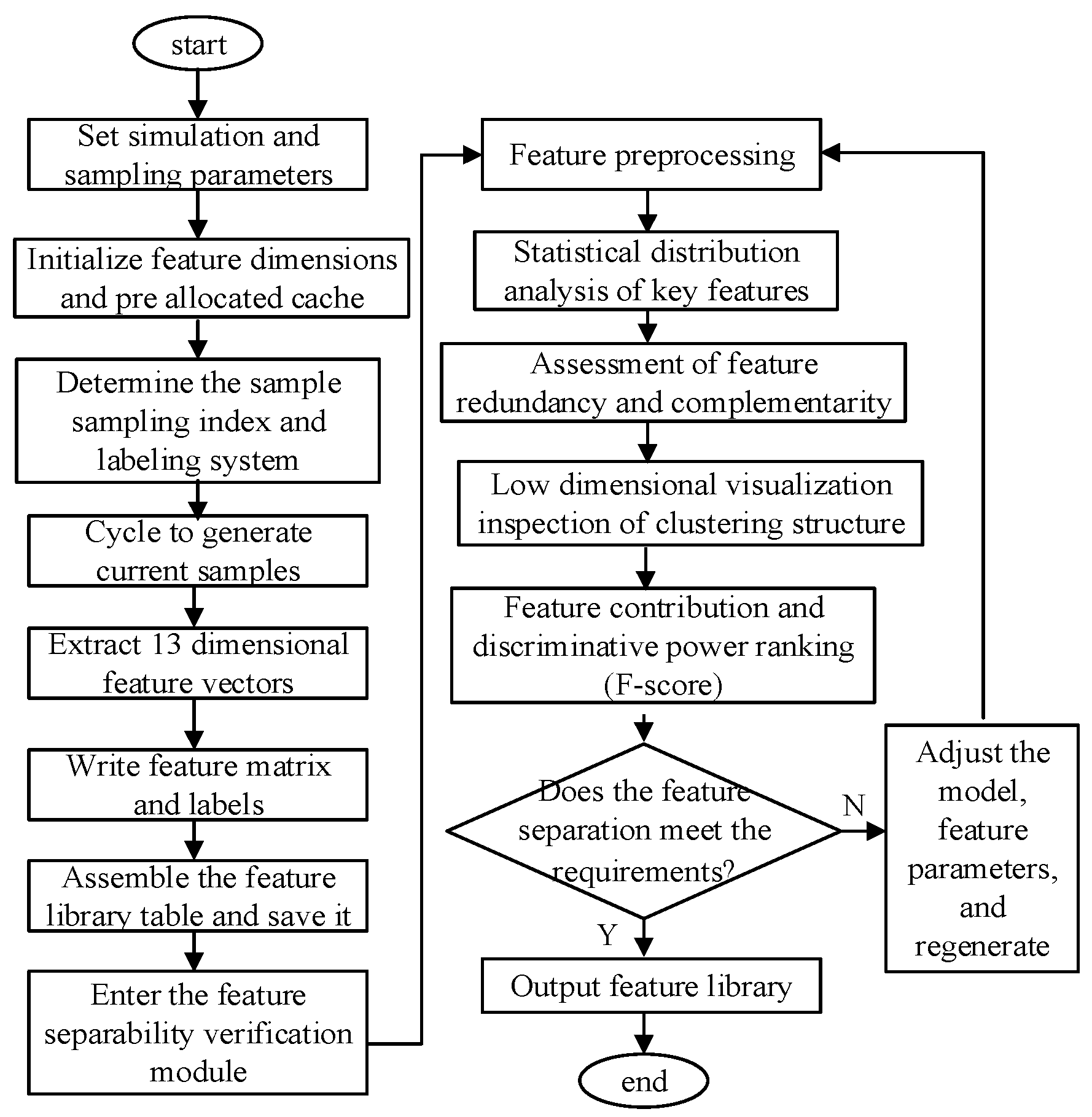
To reduce inconsistency between the training stage and the identification stage, feature fields, label encoding, normalization parameters, and category mappings are all saved as part of the model interface. When independent test samples or IEEE 33-bus access samples are later input into the model, the mean and standard deviation are not re-estimated; instead, the normalization parameters obtained during training are reused. This treatment avoids information leakage from the test set and improves the reproducibility of model deployment. The sample scale and label ranges of the feature database are summarized in Table 3.

Table 3. Sample scale of the feature database and label ranges.

Device Type	Samples per Subclass	Total Samples	Label Range
PV	1000	3000	1–3
ES	1000	3000	4–6
EV	1000	3000	7–9
IB	1000	1000	10
IF	1000	1000	11
Total	1000	11,000	1–11

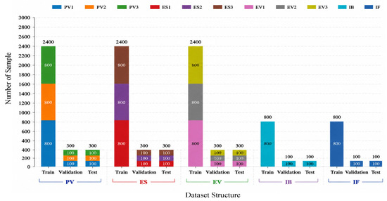
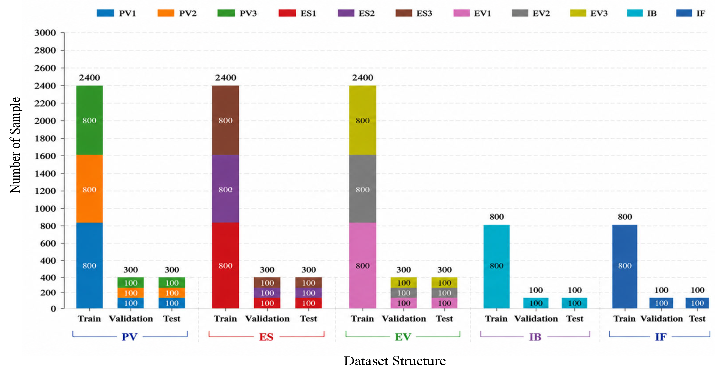
The dataset consists of five categories of distribution-network edge-end devices, including PV, ES, EV charging piles, IB, and IF devices. Considering the differences in device capacity and operating conditions, these devices are further divided into 11 subclasses. A total of 11,000 current samples are generated, and each sample is represented by a 13-dimensional current time–frequency feature vector. The dataset structure and class balance are shown in Figure 4. Since each subclass has the same number of samples, the dataset is perfectly balanced, which helps prevent classification bias and ensures a fair evaluation of the proposed identification method.

Figure 4. Class balance and dataset split of the constructed feature database.

From an engineering perspective, the value of the feature database lies not only in providing training samples but also in establishing a reusable specification for feature organization. For subsequent expansion involving new devices, calibration with measured data, or online identification systems, compatibility with the existing model can be maintained as long as the measured currents pass through the same preprocessing and feature-extraction interfaces.

3. Random-Forest-Based Identification Model for Edge-End Devices

3.1. Multi-Class Task Definition and Label Mapping

The edge-end device identification problem is formulated as an 11-class multi-class classification task. The input of each sample is a 13-dimensional feature vector, and the output is a class label yi ∈ {1, 2, …, 11}. Specifically, labels 1–3 correspond to small-, medium-, and large-capacity PV; labels 4–6 correspond to small-, medium-, and large-capacity ES; labels 7–9 correspond to slow-, fast-, and ultra-fast-charging piles; and labels 10 and 11 correspond to smart circuit breakers and intelligent fusion terminals, respectively.The corresponding label mapping is summarized in Table 4.

Table 4. Label mapping for the 11 classes of edge-end devices.

Label	Device Category	Subclass Description
1	PV	Small-Capacity PV
2	PV	Medium-Capacity PV
3	PV	Large-Capacity PV
4	ES	Small-Capacity ES
5	ES	Medium-Capacity ES
6	ES	Large-Capacity ES
7	EV	Slow Charger
8	EV	Fast Charger
9	EV	Ultra-Fast Charger
10	IB	Smart Circuit Breaker
11	IF	Intelligent Fusion Terminal

Considering the diversity of device categories and operating characteristics, 80% of the samples are used for model training to provide sufficient feature learning capability. The remaining samples are independently divided into validation and testing sets for parameter evaluation and generalization assessment. All compared classifiers use the same dataset partition strategy to ensure a fair comparison. Before model training, samples are randomly shuffled and then divided into training, validation, and test sets according to a ratio of 8:1:1. All algorithms use the same partitioning indices, and the normalization parameters are estimated only from the training set and then applied to the validation set, test set, and subsequent samples to be identified. The feature-normalization formula is

$$z_{ij}={\displaystyle \frac{x_{ij}-{\mu }_j}{{\sigma }_j}}$$

(6)

where μj and σj are the mean and standard deviation of the j-th feature in the training set, respectively. Since the features in this study include not only magnitude-based indices but also ratio-type and statistical-distribution-type indices, the dimensional scales vary significantly, and unified normalization improves the fairness of algorithm comparison.

3.2. Basic Principle of Random Forest

Random Forest is an ensemble tree model. Let the training set be D, and let the forest consist of B classification trees. For the b-th tree, a bootstrap training subset is first obtained by sampling D with replacement. Then, at each node, a subset of features is randomly selected as candidate split features, and the optimal split threshold is determined according to the Gini index or information gain. Because both sample sampling and feature sampling introduce randomness, the trees remain different from one another, and final majority voting reduces the overfitting risk of a single tree.

$$Gini(D)=1-{\displaystyle \sum _{c=1}^C{p}_c^2}$$

(7)

$$\widehat{y}=\arg {\max }_c{\displaystyle \sum _{b=1}^{B}I}\left[h_b(x)=c\right]$$

(8)

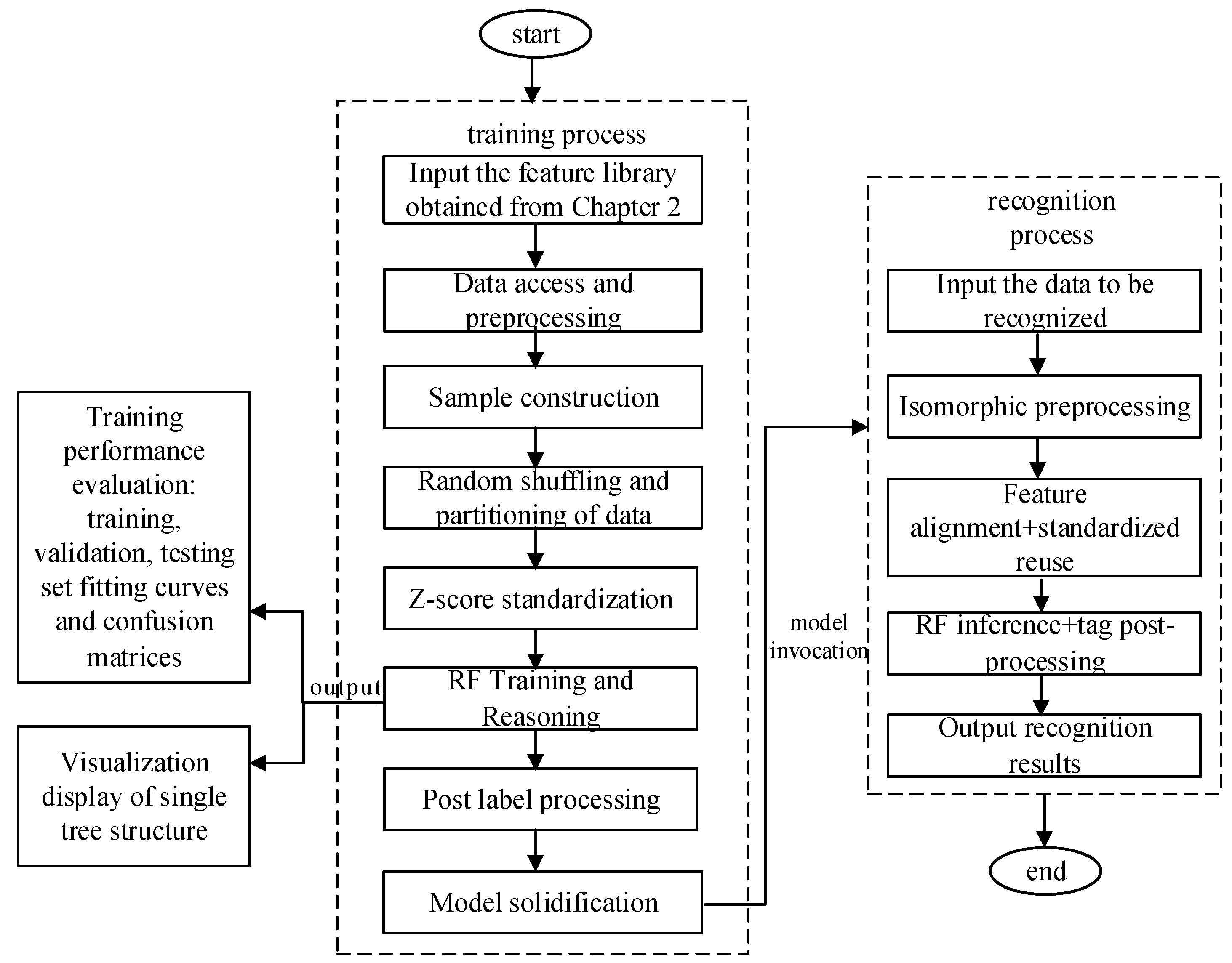
where $p_c$ represents the proportion of samples in a node that belong to class $c$, $h_b(x)$ is the classification result of the b-th tree for sample x, and $I\left[·\right]$ is the indicator function. The advantages of Random Forest are twofold: on the one hand, decision trees can characterize nonlinear classification boundaries; on the other hand, multi-tree voting reduces the sensitivity of a single partition rule to noisy samples. Moreover, the model can interpret its identification basis through feature importance and local splitting paths, which is meaningful for edge-side applications in distribution networks.The RF-based identification workflow is illustrated in Figure 5.

Figure 5. Edge-end device identification workflow based on Random Forest.

3.3. Comparison of the Applicability of Different Algorithms

To explain why Random Forest is selected, this paper also compares five multi-class algorithms: k-NN, Naive Bayes, SVM, BP/MLP, and RF. These correspond to typical classification paradigms based on distance measurement, probabilistic discrimination, maximum-margin separation, and back-propagation learning, respectively [17,18,19,20]. k-NN does not require explicit training, but during inference it must compute the distances between a query sample and all training samples, leading to high deployment cost when the sample scale is large or edge-side computing power is limited. Naive Bayes is computationally efficient, but its conditional-independence assumption is not fully consistent with the correlated features considered here. SVM has strong boundary-modeling capability, but its performance depends on the kernel function, penalty factor, and multi-class strategy. BP/MLP offers strong representation ability, but it is sensitive to sample scale, network architecture, and initialization.

As shown in Table 5, RF does not dominate every single criterion but achieves a relatively balanced performance in terms of accuracy, robustness, interpretability, and deployment cost. For the 13-dimensional current features considered in this study, class boundaries are somewhat nonlinear, and some features are correlated. Therefore, RF is more suitable as the core identifier than linear classifiers or probabilistic models relying on strong assumptions.

Table 5. Applicability comparison of common multi-class algorithms.

Algorithm	Expressive Power	Robustness	Interpretability	Engineering Cost	Applicability Conclusion
k-NN	Medium	Medium-Low	Low	High inference cost	Sensitive to boundaries and noise; unfavorable for deployment
Naive Bayes	Medium-Low	Medium	Medium-High	Low	Suitable as a fast baseline, but the upper bound is limited by the feature-independence assumption
SVM	Medium-High	Medium	Medium-Low	Medium-High	System parameter tuning is required, and category concentration is prone to occur when there is overlap between categories
BP/MLP	High	Data-dependent	Low	High	Sensitive to parameters and samples; higher engineering-maintenance cost
RF	High	Medium-High	Medium-High	Medium	Balanced overall performance; well suited to 13-dimensional tabular features

3.4. Interface Design Ensuring Consistency Between Training and Identification

In practical deployment, an identification model often needs to continuously receive current data from different sensing terminals and different time periods. If the data-processing workflow is inconsistent between training and identification, even a highly accurate classifier may show evident deviations in real applications. Therefore, interface consistency is treated as a key part of model construction in this paper. The data-interface design is summarized in Table 6.

Table 6. Data-interface design ensuring consistency between training and identification.

Module	Input	Output	Function
Data Reading	Raw current sequence or feature table	Sample table with unified fields	Ensures consistency of feature order, label fields, and missing-value processing
Feature Extraction	Current sequence i(t)	13-D feature vector	Computes time-domain, frequency-domain, and time–frequency fluctuation indices
Normalization	Training-set feature matrix	μ, σ, and normalized features	Fixes the training scale and avoids test-set information leakage
Model Training	Normalized training samples	RF model object	Obtains multiple classification trees and voting rules
Label Mapping	Numerical labels	Device-category names	Converts model outputs into engineering-readable results
Identification Invocation	Current samples to be identified	Category, confidence, and evaluation indices	Performs online or offline device identification

The normalization parameters and label mappings must be solidified and stored together with the trained RF model. For newly acquired samples, the system first performs the same feature extraction, then uses the μ and σ obtained during training to complete scale transformation and finally feeds the result into the RF model to obtain the class output. This treatment reduces scale drift across different batches of samples and also facilitates later embedding of the model into edge-side sensing terminals.

To facilitate complete reproduction of the experimental workflow in a journal paper, the identification method is summarized into two stages: offline training and online identification. The offline stage completes sample-database construction, feature normalization, model training, and validation; the online stage performs only current-window extraction, feature extraction, fixed-parameter normalization, and model invocation. The two stages share the same feature names, feature order, and label mappings, thereby avoiding identification errors caused by field misalignment or re-estimation of scaling parameters.

In terms of evaluation metrics, in addition to overall accuracy, Precision, Recall, and F1-score are calculated for each class. For a given class c, Precision reflects the proportion of samples predicted as class c that truly belong to class c; Recall reflects the proportion of true class-c samples that are correctly identified; and the F1-score is used to comprehensively measure the balance between the two.

$$Precisio{n}_c={\displaystyle \frac{T{P}_c}{T{P}_c+F{P}_c}},\hspace{1em}\hspace{1em}Recal{l}_c={\displaystyle \frac{T{P}_c}{T{P}_c+F{N}_c}}$$

(9)

$$F{1}_c={\displaystyle \frac{2Precisio{n}_c\cdot Recal{l}_c}{Precisio{n}_c+Recal{l}_c}}$$

(10)

Considering the diversity of device categories and operating characteristics, 80% of the samples are used for model training to provide sufficient feature learning capability. The remaining samples are independently divided into validation and testing sets for parameter evaluation and generalization assessment. All compared classifiers use the same dataset partition strategy to ensure a fair comparison.

Table 7 summarizes the implementation workflow of the proposed RF-based edge-end device identification method, covering offline model training and online identification stages.

Table 7. Implementation steps of RF-based edge-end device identification.

Step	Stage	Key Processing	Output
1	Offline Training	Generate current samples for 5 categories and 11 subclasses in batches and extract 13-dimensional features	Feature sample table
2	Offline Training	Split training, validation, and test samples at 8:1:1	Data indices and labels
3	Offline Training	Estimate mean μ and standard deviation σ from the training set and complete normalization	Normalization parameters
4	Offline Training	Train the RF classifier and save the model, label mapping, and feature order	Identification-model file
5	Online Identification	Apply the same window extraction and feature extraction to the current to be identified	Feature vector to be identified
6	Online Identification	Normalize using μ and σ saved during training	Normalized input features
7	Online Identification	Input into the RF model and output the category according to the voting result	Device category and evaluation results

4. Feature Separability and Model Identification Results

4.1. Statistical Distribution Analysis of Key Features

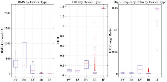
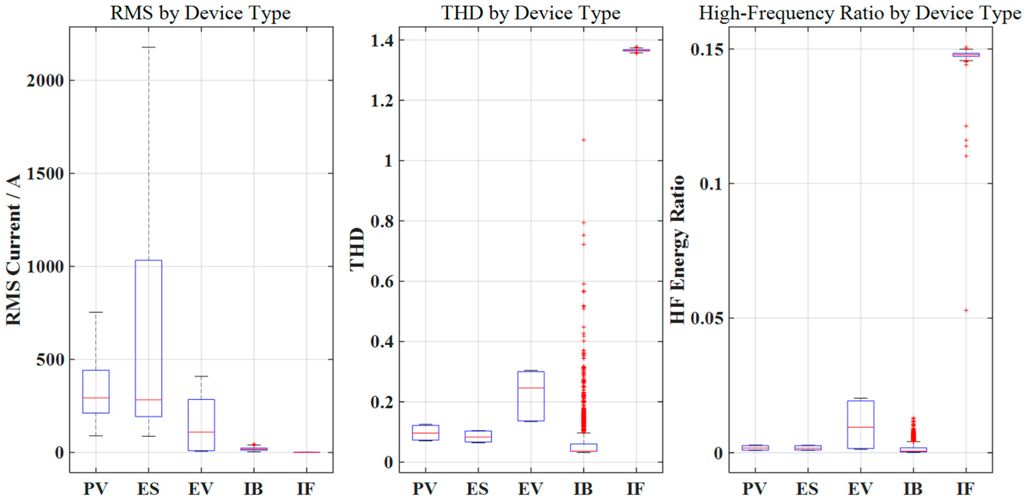
Feature separability is first analyzed intuitively by boxplots. Figure 6 presents the statistical distributions of several key features for different device classes. The red “+” symbols denote outliers beyond the whiskers. RMS and the fundamental amplitude mainly reflect device capacity or power rating and are sensitive to high-power devices such as PV, ES, and EV. THD reveals the non-sinusoidal distortion introduced by power-electronic interfaces. HF_ratio is sensitive to inverter ripple, converter ripple, and the switching ripple of terminal power supplies. RMS_CV reflects amplitude fluctuation within a short time window and supplements the description of energy-storage ramps, charging-stage transitions, and circuit-breaker surges.

Figure 6. Statistical comparison of key features.

From the distribution patterns, IF generally has a relatively clear boundary in terms of high-frequency energy ratio and harmonic structure. IB has a relatively low overall amplitude, but when breaker samples contain switching surges, peak-related and kurtosis-related indices exhibit greater dispersion. PV, ES, and EV show local overlap, which is related to the fact that all three types are connected through power-electronic interfaces. Therefore, subsequent identification should not rely on any single feature alone but rather form class boundaries through multi-dimensional feature fusion.

4.2. Analysis of Feature Redundancy and Complementarity

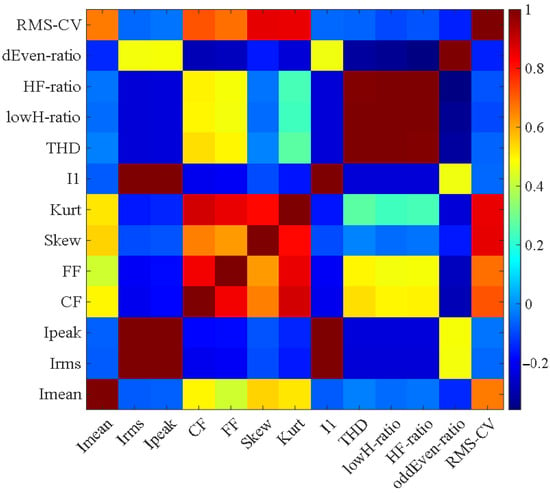
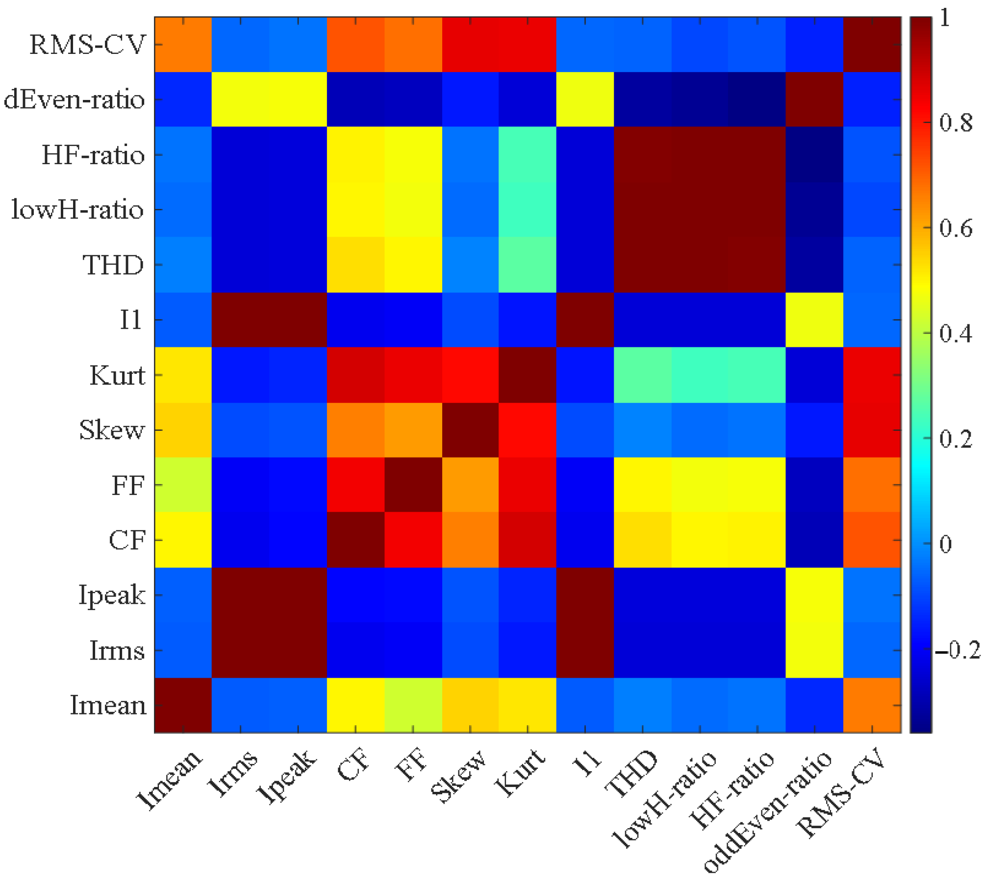
To determine whether the 13-dimensional features contain obvious redundancy, the feature-correlation matrix is further calculated, as shown in Figure 7. The amplitude-related indices exhibit high correlation, indicating that they jointly reflect current magnitude. The harmonic-related and high-frequency-related features are not fully consistent with the amplitude-related features and can therefore provide additional spectral-structure information. RMS_CV, skewness, kurtosis, and similar indices have relatively weak correlation with most magnitude-related features, showing that they mainly describe local waveform variations and distributional shape.

Figure 7. Correlation matrix of the 13-dimensional features.

The correlation analysis indicates that the 13-dimensional feature system contains both a certain degree of redundancy and clear complementarity. Moderate redundancy helps improve model stability under noise disturbances, while complementary features enhance the fine-grained discrimination of similar categories. For example, a slow charger and a smart circuit breaker may have similar RMS values but may still differ in low-order harmonic energy, high-frequency ripple, and short-term fluctuations. When the amplitude ranges of medium-capacity ES and large-capacity PV overlap, low-order harmonic and high-frequency energy features can provide further partitioning cues for Random Forest.

4.3. Low-Dimensional Visualization and Ranking of Feature Contributions

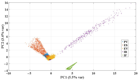
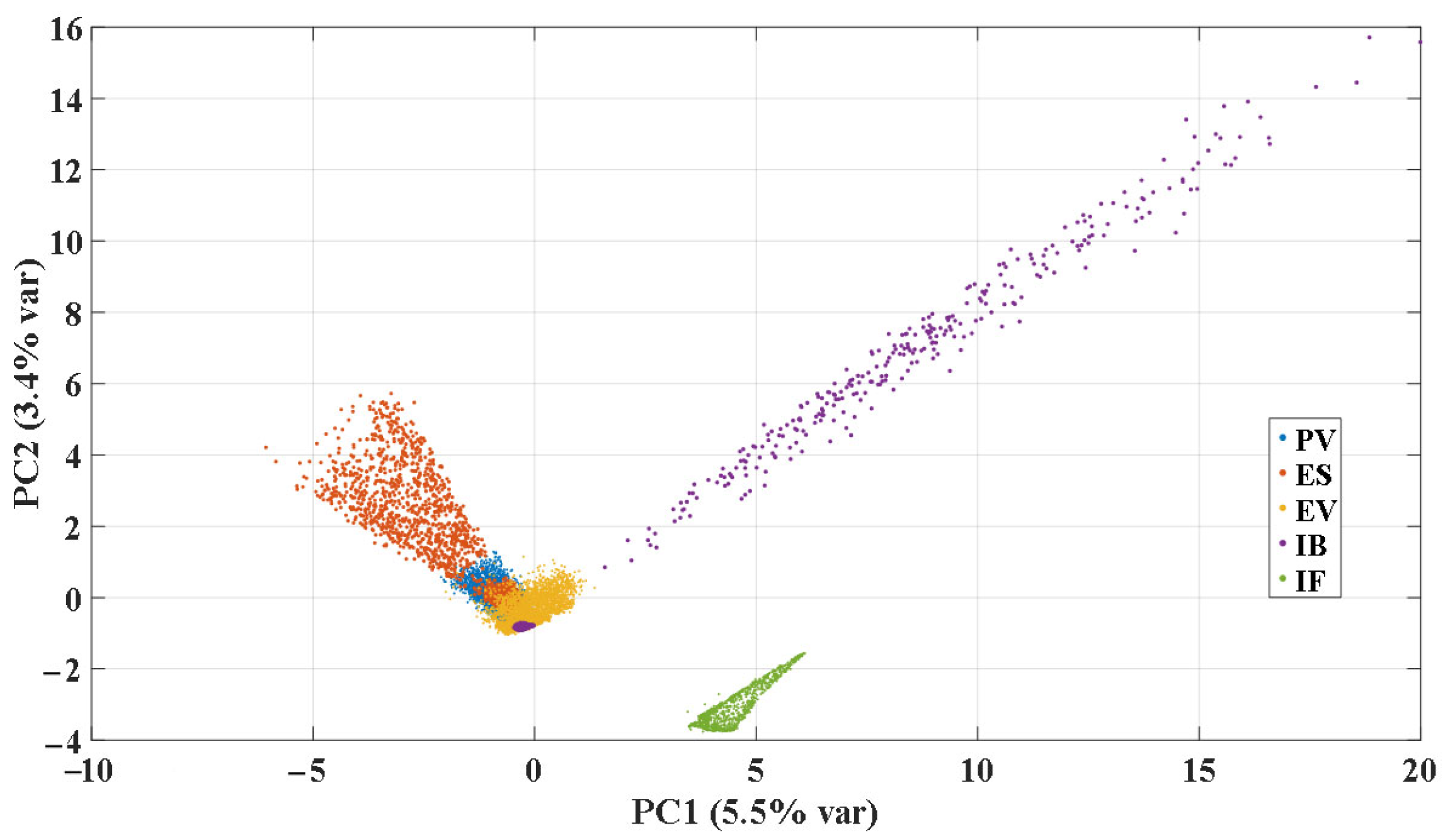
To observe the overall clustering structure in the multi-dimensional feature space, PCA is used to project the 13-dimensional features onto a two-dimensional plane. Figure 8 shows that IB and IF are relatively far from PV, ES, and EV, indicating obvious differences between intelligent-terminal-type devices and high-power power-electronic devices. PV, ES, and EV overlap in some local regions, suggesting the existence of similar boundaries in their current features. This phenomenon is also consistent with the later misclassification distribution observed in the confusion matrix.

Figure 8. PCA two-dimensional projection colored by major device category.

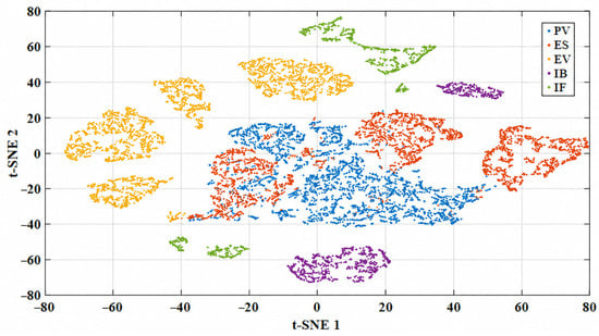
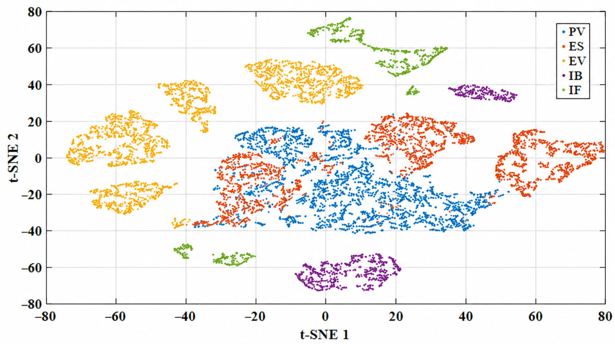
Due to the certain limitations of linear projection, this section further presents the two-dimensional embedding results of t-SNE, as shown in Figure 9.

Figure 9. t-SNE two-dimensional projection colored by major device category.

As can be observed from the figure, the clustering boundaries for different equipment types in the local space are more distinct than those obtained from PCA. Although certain regions still exhibit proximity among PV, ES, and EV, based on the overall distribution, these three groups have formed relatively independent cluster structures. This indicates that, when multiple features are combined, the model can demonstrate stronger discriminative capability in the nonlinear space, as well as exhibit favorable feature separation potential.

Table 8 shows that HF_ratio, the low-order harmonic energy ratio, and THD rank at the top, indicating that frequency-domain energy distribution is an important basis for distinguishing edge-end devices. Magnitude-related features rank in the middle and still contribute to identifying capacity levels. Although fluctuation-related features such as RMS_CV rank relatively lower, they provide useful supplementary information for a few difficult-to-distinguish categories. Considering both contribution ranking and engineering interpretability, all 13 features are retained as the input of the identification model.

Table 8. F-score ranking of the 13 features and their roles.

Rank	Feature	F-Score	Role Description
1	HF_ratio	285,028.595	Distinguishes power-electronic ripple from terminal switch-mode-power-supply characteristics
2	lowH_ratio	274,761.434	Characterizes differences in low-order harmonic structure
3	THD	160,235.807	Measures differences in total harmonic distortion
4	CrestFactor	1632.464	Captures spike and surge characteristics
5	oddEven_ratio	1553.051	Separation of odd and even harmonic features
6	FormFactor	1235.015	Describes waveform-shape differences
7	I1	1213.528	Reflects fundamental amplitude and capacity level
8	Irms	1194.910	Reflects RMS current magnitude
9	Ipeak	1093.136	Characterizes peaks and local surges
10	Kurtosis	767.014	Reflects peakedness
11	RMS_CV	739.707	Reflects short-window amplitude fluctuation
12	Skewness	565.169	Reflects the degree of distributional skewness
13	Imean	418.919	Reflects DC bias and asymmetry

4.4. Comparison of Identification Results Among Multiple Algorithms

Under the same dataset, the same random partition, and the same preprocessing workflow, k-NN, Naive Bayes, SVM, BP/MLP, and RF are trained separately. The main parameters and training settings of the evaluated classifiers are summarized in Table 9. All classifiers were implemented in MATLAB R2025a.

Table 9. Hyper-parameter settings of different classifiers.

Model	MATLAB Function	Key Hyper-Parameters
k-NN	fitcknn	NumNeighbors = 1, Distance = ‘euclidean’
Naive Bayes	fitcnb	DistributionNames = ‘normal’
SVM	fitcecoc	KernelFunction = ‘rbf’, BoxConstraint = 1
BP/MLP	fitcnet	LayerSizes = [10], Activations = ‘relu’, Solver = ‘adam’
RF	TreeBagger	NumTrees = 50, MinLeafSize = 1

The internal train-test results show that all five algorithms can achieve a certain degree of fitting on the same feature database. However, when independent regenerated test samples are used to examine generalization performance, obvious differences emerge among the algorithms.

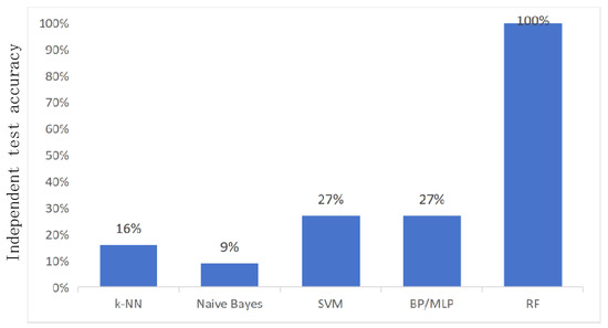
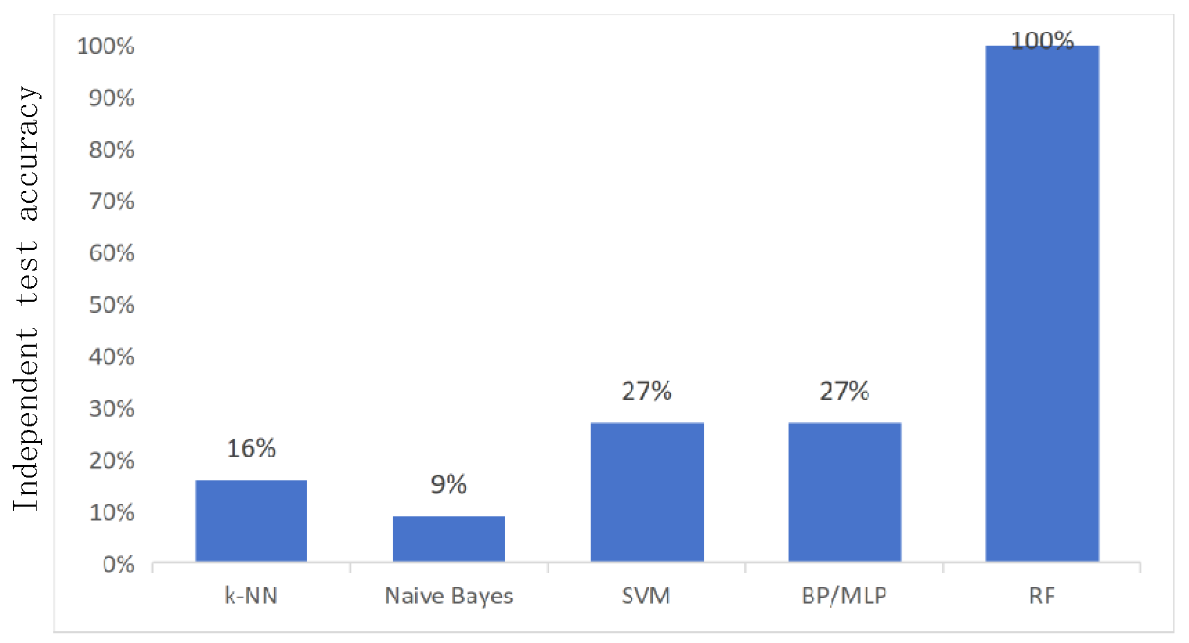
Figure 10 shows that the overall accuracies of k-NN and Naive Bayes on independent test samples are approximately 16% and 9%, respectively, and a large number of samples are concentratedly misclassified as smart circuit breakers, indicating that these two methods are sensitive to class-boundary overlap and feature correlation. The accuracies of SVM and BP/MLP are both around 27%; although they can correctly identify some samples, significant category-concentration misclassification still exists. By contrast, RF achieves an overall accuracy above 98%, which is substantially better than the other models.

Figure 10. Comparison of independent-test accuracies of the five identification algorithms.

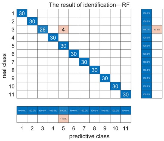
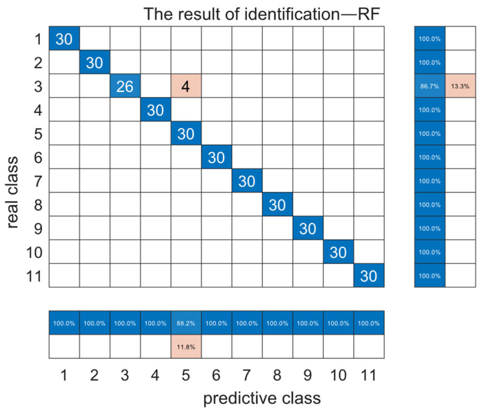
The identification performance of different classifiers is first compared using the same feature vectors and dataset partition strategy. As shown in Table 10, Random Forest achieves the highest overall accuracy among the evaluated models. For k-NN, the F1-score is lower than accuracy, indicating that the misclassifications are unevenly distributed across device categories, with most samples concentrated in a few classes.As shown in Figure 11, most device categories are correctly identified, and the main misclassifications occur between large-capacity PV and medium-capacity ES.

Table 10. Independent-test performance of different classifiers and major misclassification patterns.

Model	Accuracy	Precision	Recall	F1-Score	Main Misclassification Pattern
k-NN	16.1%	19.1%	16.1%	11.4%	A large number of samples are concentratedly misclassified as IB
Naive Bayes	9.1%	0.9%	9.1%	1.6%	Most categories are misclassified as IB
SVM	27.3%	19.2%	27.3%	20.0%	Misclassifications are concentrated in a few ES categories
BP/MLP	27.3%	20.0%	27.3%	21.2%	Marked confusion between large-capacity ES and IB
RF	98.8%	98.9%	98.7%	98.8%	Minor confusion between similar PV and ES categories

Figure 11. Confusion matrix of edge-end device identification based on RF.

From the RF confusion matrix, most device categories can be correctly identified, and the main misclassifications are concentrated between large-capacity PV and medium-capacity ES. This phenomenon is physically reasonable: under some operating conditions, the two device classes may have similar current magnitudes, low-order harmonic distributions, and high-frequency ripple intensities, while random disturbances further compress the feature interval. By contrast, intelligent fusion terminals exhibit more pronounced high-frequency ripple and even-order harmonic features, leading to a relatively clear identification boundary.

5. Case Validation in the IEEE 33-Bus Access Scenario

5.1. Case Setup

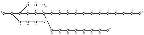
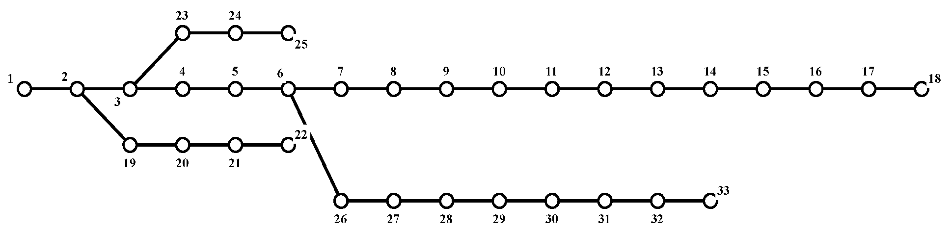
Validation with independent samples can demonstrate the separability of device current features themselves, but actual measurements in distribution networks usually occur at specific nodes or branches. To further verify the applicability of the method, an IEEE 33-bus distribution-network case is constructed based on case33bw in MATPOWER 8.0. After edge-end devices are connected to a node, the measured current is jointly affected by node voltage, background load, and network power-flow states, which is closer to the actual acquisition conditions of sensing units.The topology of the IEEE 33-bus distribution network is shown in Figure 12.

Figure 12. Topology of the IEEE 33-bus distribution network.

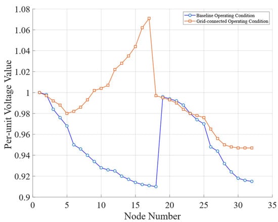
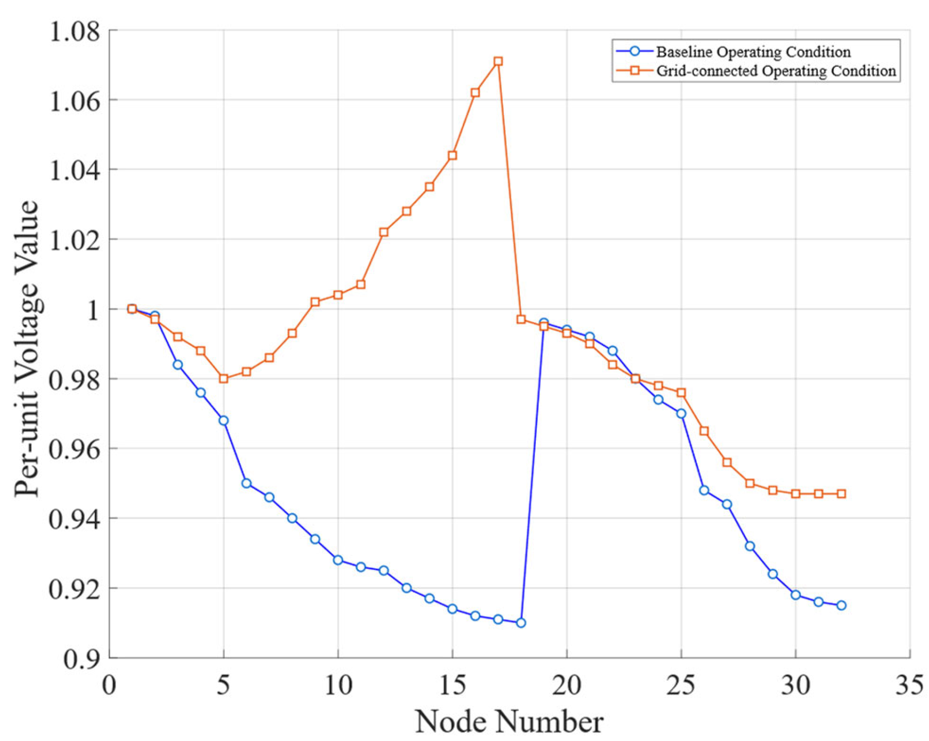
In the supplementary case, 100 node-access samples are generated for each category. Taking the case of a medium-capacity PV connected to node 18 as an example, the voltage distribution changes before and after connection, indicating that the sample-generation process already considers the network operating background rather than simply copying isolated device waveforms.

5.2. Identification Results and Confusion Analysis

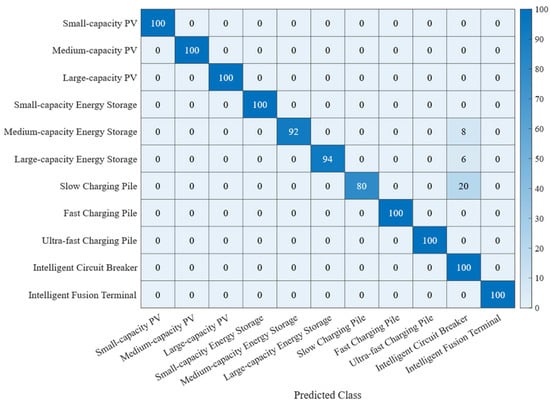
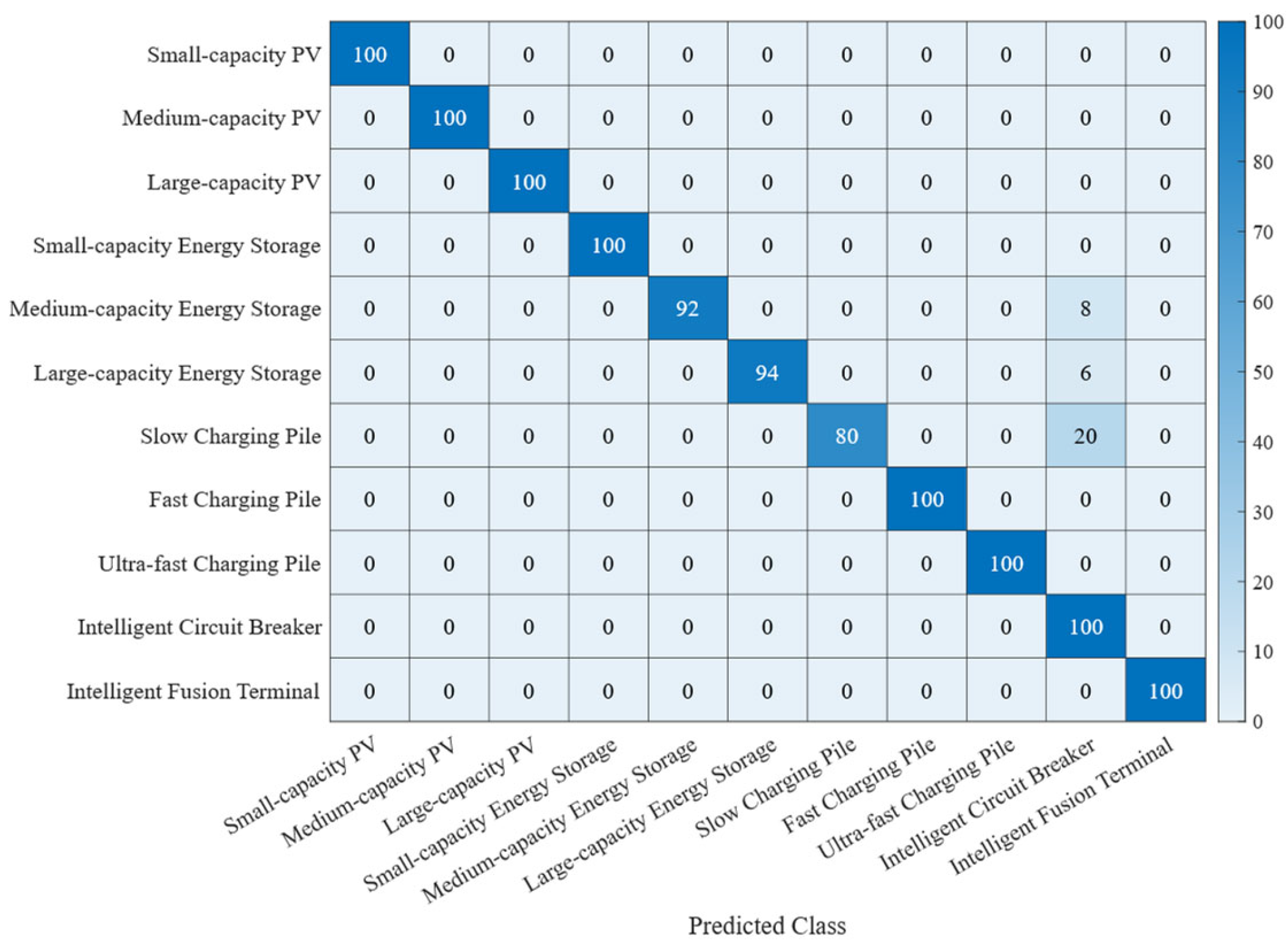
The voltage profiles before and after connecting a medium-capacity PV at node 18 are compared in Figure 13. Figure 14 indicates that the three PV categories, small-capacity ES, fast chargers, ultra-fast chargers, smart circuit breakers, and intelligent fusion terminals are all correctly identified. Misclassifications mainly occur among medium-capacity ES, large-capacity ES, and slow chargers versus smart circuit breakers. This is because some ES devices operating at low power or under slow charging/discharging ramps may exhibit low-order harmonics, high-frequency ripple, and magnitude characteristics similar to those of other power-electronic-interface devices. In addition, slow chargers have relatively low rated power, and under steady charging their current magnitudes may approach those of certain low-voltage loads or downstream currents of smart circuit breakers, making them more likely to be classified into the IB category.

Figure 13. Voltage comparison before and after connecting a medium-capacity PV at node 18.

Figure 14. Confusion matrix of edge-end device identification in the IEEE 33-bus access scenario.

Table 11 shows that the overall identification accuracy in the IEEE 33-bus access case reaches 96.91%, and the overall Precision, Recall, and F1-score remain at relatively high levels. This result indicates that when the identification scenario is extended from independent device samples to the distribution-network node-access background, the 13-dimensional current features constructed in this paper can still effectively characterize the current characteristics of different devices, and the Random Forest model also maintains good scenario adaptability.

Table 11. Evaluation indices of edge-end device identification in the IEEE 33-bus access scenario.

Device Category	Precision	Recall	F1
Small-Capacity PV	1.000	1.000	1.000
Medium-Capacity PV	1.000	1.000	1.000
Large-Capacity PV	1.000	1.000	1.000
Small-Capacity ES	1.000	1.000	1.000
Medium-Capacity ES	1.000	0.920	0.958
Large-Capacity ES	1.000	0.940	0.969
Slow Charger	1.000	0.800	0.889
Fast Charger	1.000	1.000	1.000
Ultra-Fast Charger	1.000	1.000	1.000
Smart Circuit Breaker	0.746	1.000	0.855
Intelligent Fusion Terminal	1.000	1.000	1.000
Overall	0.969	0.969	0.970

5.3. Discussion of Engineering Applicability

From an engineering perspective, the proposed method provides a low-dimensional and interpretable framework for edge-end device identification. For terminals with sufficient sampling capability, current acquisition and feature extraction can be performed locally, and only the extracted 13-dimensional feature vectors need to be transmitted instead of complete waveforms, reducing communication and storage requirements. For resource-limited terminals, waveform data can be uploaded to edge nodes or master stations for centralized identification.

However, the proposed framework is mainly designed for dominant single-device identification under short-time steady-state conditions. When multiple devices operate simultaneously at the same node, the measured current becomes a superposition of multiple device currents, which cannot be fully represented by the current single-label classification model. Moreover, practical distribution networks may involve voltage distortion, background harmonics, impedance variations, topology changes, measurement noise, and device-parameter dispersion, which may introduce additional variations into the extracted features.

In addition, the IEEE 33-bus case considers different installation locations and network impedance conditions, demonstrating the applicability of the proposed method under typical distribution-network scenarios. Future work will focus on improving robustness through expanded operating-condition datasets, adaptive feature compensation, multi-device identification, and online incremental learning.

6. Conclusions

This paper addresses the identification of edge-end devices in distribution networks under the background of distributed-resource integration, and proposes a method based on current time–frequency features and Random Forest. The method is validated using both feature-database case studies and the IEEE 33-bus access scenario. The main conclusions are as follows:

(1) After establishing equivalent grid-connected current models for PV, ES, EV, IB, and IF, a 13-dimensional current feature system is constructed using information on magnitude, waveform shape, harmonics, high-frequency ripple, and short-window fluctuations, which can relatively comprehensively express the current differences among various edge-end devices. The F-score ranking and low-dimensional visualization results show that the high-frequency energy ratio, low-order harmonic energy ratio, and THD contribute most to device discrimination, while magnitude-related and fluctuation-related features play important supplementary roles.

(2) Under a unified preprocessing, label-mapping, and normalization workflow, Random Forest exhibits better generalization on independent samples than k-NN, Naive Bayes, SVM, and BP/MLP. RF achieves an overall accuracy above 98% on independent test samples, can effectively describe the nonlinear boundaries among the 11 classes of edge-end devices in the feature space, and can provide a certain degree of interpretability through feature importance and tree-structure paths.

(3) The IEEE 33-bus access case shows that the proposed method remains applicable under the background of actual network operation, with an overall identification accuracy of 96.91%. Local confusion still exists among slow chargers, some ES categories, and smart circuit breakers. Future work may further improve model generalization in complex operating conditions by incorporating more field-measured samples, node-voltage information, power-disturbance features, and online updating mechanisms.

In terms of the application boundary, the proposed method is more suitable for identification scenarios with a single node, a dominant single class of device, or clearly dominant features. When multiple edge-end devices are connected to the same node, the node current exhibits multi-source superposition characteristics, and a single-label classifier will lose part of the combination information if it outputs only one device type. Future work may introduce multi-label learning, event decomposition, and probabilistic modeling of device combinations on top of the present feature system, thereby extending the identification result from “determining a single class” to “estimating the device combination and its contribution ratio”.

At the same time, the samples in this study are mainly based on simulation models and supplementary network cases and do not yet cover all field device parameters, sampling noise, and long-term operating variations. For engineering applications, it is recommended to use measured data from actual transformer districts as secondary calibration samples, periodically update the RF model, and jointly verify the identification results with voltage, power, and node-topology information so as to improve the credibility of the model in complex operating environments.

References

- Shu, Y.; Tang, Y.; Zhang, Z.; Zhang, F.; Yang, L.; Zhong, W.; Gu, Z. Construction of New Distribution Network and Its Key Technologies. Chin. J. Electr. Eng. 2024, 44, 6721–6733. [Google Scholar]
- Ruan, G.; He, Y.; Tan, Z.; Zhong, H. Overview of Data Physical Fusion Modeling for the Operation of New Power Systems. Chin. J. Electr. Eng. 2024, 44, 5021–5036. [Google Scholar]
- Wang, P.; Lin, J.; Ning, X.; Guo, S.; Zhang, J.; Fang, M. Design of Panoramic Information Perception Architecture for Distribution Network. High Volt. Technol. 2021, 47, 2293–2302. [Google Scholar]
- Hart, G.W. Nonintrusive appliance load monitoring. Proc. IEEE 1992, 80, 1870–1891. [Google Scholar] [CrossRef] [Scilit]
- Deng, X.P.; Zhang, G.Q.; Wei, Q.L.; Peng, W.; Li, C.D. A survey on the non-intrusive load monitoring. Acta Autom. Sin. 2022, 48, 644–663. [Google Scholar]
- Schirmer, P.A.; Mporas, I. Non-intrusive load monitoring: A review. IEEE Trans. Smart Grid 2023, 14, 769–784. [Google Scholar] [CrossRef] [Scilit]
- Tanoni, G.; Principi, E.; Squartini, S. Non-intrusive load monitoring in industrial settings: A systematic review. Renew. Sustain. Energy Rev. 2024, 202, 114703. [Google Scholar] [CrossRef] [Scilit]
- Luan, K.; Yang, S.; Huang, Y.; Fang, K.; Cheng, H.; Huang, S. Research on Fisher SVM Feature Selection based load identification. J. Electr. Power Sci. Technol. 2023, 38, 230–239+264. [Google Scholar]
- Breiman, L. Random forests. Mach. Learn. 2001, 45, 5–32. [Google Scholar] [CrossRef] [Scilit]
- Ho, T.K. The random subspace method for constructing decision forests. IEEE Trans. Pattern Anal. Mach. Intell. 1998, 20, 832–844. [Google Scholar] [CrossRef] [Scilit]
- Geurts, P.; Ernst, D.; Wehenkel, L. Extremely randomized trees. Mach. Learn. 2006, 63, 3–42. [Google Scholar] [CrossRef] [Scilit]
- Scornet, E.; Biau, G.; Vert, J.-P. Consistency of random forests. Ann. Stat. 2015, 43, 1716–1741. [Google Scholar] [CrossRef] [Scilit]
- Wang, J.; Yi, S.; Liu, J.; Liu, J. Non intrusive industrial load identification based on random forest algorithm and steady-state waveform. China Electr. Power 2022, 55, 82–89. [Google Scholar]
- Zhao, Z.; Bi, T.; Ren, Q.; Shao, Y.; Ren, J. Research on Non invasive Industrial Load Identification and Its Robustness Based on Wavelet Random Forest. Water Resour. Hydropower Technol. 2022, 53, 265–270. [Google Scholar]
- Brenna, M.; Foiadelli, F.; Leone, C.; Longo, M. Electric vehicles charging technology review and optimal size estimation. J. Electr. Eng. Technol. 2020, 15, 2539–2552. [Google Scholar] [CrossRef] [Scilit]
- Tahir, M.U.; Sangwongwanich, A.; Stroe, D.-I.; Blaabjerg, F. Overview of multi-stage charging strategies for Li-ion batteries. J. Energy Chem. 2023, 84, 228–241. [Google Scholar] [CrossRef] [Scilit]
- Cover, T.M.; Hart, P.E. Nearest neighbor pattern classification. IEEE Trans. Inf. Theory 1967, 13, 21–27. [Google Scholar] [CrossRef] [Scilit]
- Zhang, H. The optimality of naive Bayes. In Proceedings of the Seventeenth International Florida Artificial Intelligence Research Society Conference; AAAI Press: Menlo Park, CA, USA, 2004; pp. 562–567. [Google Scholar]
- Cortes, C.; Vapnik, V. Support-vector networks. Mach. Learn. 1995, 20, 273–297. [Google Scholar] [CrossRef] [Scilit]
- Rumelhart, D.E.; Hinton, G.E.; Williams, R.J. Learning representations by back-propagating errors. Nature 1986, 323, 533–536. [Google Scholar] [CrossRef] [Scilit]
Disclaimer/Publisher’s Note: The statements, opinions and data contained in all publications are solely those of the individual author(s) and contributor(s) and not of MDPI and/or the editor(s). MDPI and/or the editor(s) disclaim responsibility for any injury to people or property resulting from any ideas, methods, instructions or products referred to in the content. |
© 2026 by the authors. Licensee MDPI, Basel, Switzerland. This article is an open access article distributed under the terms and conditions of the Creative Commons Attribution (CC BY) license.