Observer Pre-Synchronization for Smooth Transition in Wide-Speed-Range Sensorless Control of IPMSM Drives

Abstract

To reduce transition disturbances in wide-speed-range sensorless control of interior permanent magnet synchronous motor (IPMSM) drives, this paper proposes an observer pre-synchronization method for the transition between a low-speed high-frequency-injection (HFI) estimator and an active-flux observer used in the medium- and high-speed regions. The HFI estimator maintains position observability at standstill and low speeds, whereas the active-flux observer estimates rotor position and speed at higher speeds while accounting for IPMSM saliency. However, when the active-flux observer runs in the background at low speed, its estimated angle may not be sufficiently aligned with the HFI-estimated angle before the transition, which can cause angle discontinuities and speed fluctuations. To reduce this initial angular mismatch, the HFI-estimated rotor position is used to construct a reference active-flux vector and correct the observer state before the transition interval. A speed-dependent sigmoid weighting factor is then introduced to smoothly blend the two estimated angle vectors and scale the HFI voltage amplitude during the transition. The paper first establishes the HFI and active-flux estimation models, then formulates the observer pre-synchronization and smooth-transition strategy, and finally validates the proposed method experimentally. Experimental results show that the proposed method improves the alignment between the two estimators before the transition and reduces angle and speed transients, thereby improving transition smoothness in the IPMSM sensorless drive.

1. Introduction

Interior permanent magnet synchronous motor (IPMSM) drives are widely employed in electric vehicles, servo systems, and high-performance industrial applications owing to their high torque density, high efficiency, and wide constant-power speed range [1,2,3,4,5]. Field-oriented control requires accurate rotor position and speed information. Although this information can be obtained using a mechanical position sensor, the sensor increases the cost and size of the drive and reduces its reliability in harsh environments. Sensorless operation is therefore desirable for IPMSM drives.

Sensorless methods for IPMSMs are generally classified into signal-injection and fundamental-model-based approaches. At standstill and low speed, the back electromotive force (back-EMF) is insufficient for reliable model-based estimation. High-frequency injection (HFI) methods instead extract the rotor position from the saliency- or saturation-dependent current response [6,7,8,9]. Square-wave voltage injection is particularly attractive because of its simple implementation and high estimation bandwidth [6,7,8,9]. Further studies have improved the practical performance of square-wave HFI by mitigating inverter-induced voltage distortion, compensating estimation errors under low switching frequencies and digital delays, and suppressing position harmonics associated with high-frequency injection [10,11,12]. However, continuous injection may introduce additional current ripple and acoustic noise and may reduce the voltage margin available for the fundamental voltage output [9]. Therefore, the HFI voltage should be gradually reduced and eventually removed as the speed increases.

At medium and high speeds, the increased back-EMF enables reliable position estimation from the fundamental stator voltage and current. Extended-state observers, sliding-mode observers, phase-locked loops (PLLs), and flux observers have been extensively investigated for this purpose [13,14]. Existing studies have further advanced adaptive and nonlinear flux observers through systematic analyses of convergence, robustness, and transient behavior, strengthening the theoretical and practical basis of model-based IPMSM position estimation [15,16,17]. For an IPMSM, the rotor saliency couples the permanent-magnet flux and the reluctance component. The active flux formulation combines these position-dependent terms into a single vector aligned with the rotor magnetic axis [18,19]. Active flux estimation and its robustness against observer and parameter errors have consequently received considerable attention [19,20,21]. Nevertheless, the accuracy of a fundamental-model-based observer deteriorates at low speed, and a hybrid estimation structure is required for operation over a wide speed range.

Hybrid sensorless control combines the reliable low-speed position information provided by HFI with model-based estimation at higher speeds. Existing strategies include direct switching, speed-dependent output weighting, and hybrid observer structures [22,23,24,25,26,27]. Direct switching is sensitive to angular mismatch between the estimators, whereas weighting-based and hybrid methods introduce an overlap region to improve output continuity. However, output continuity does not ensure that the internal state of an independently operating model-based observer is aligned with the HFI estimate before blending begins. An initial phase mismatch may therefore remain at the lower transition boundary and produce position and speed transients during the transition.

This paper addresses this state-alignment problem by pre-synchronizing the active flux observer with the HFI estimate before output blending. Unlike output-only transition methods, the proposed correction acts directly on the observer state in the low-speed region. During low-speed operation, the HFI angle is used to construct a reference active flux vector, and an orthogonal correction term is added to the observer dynamics. The observer state is thus aligned before the drive enters the transition region. A sigmoid weighting function then blends the two unit position vectors and simultaneously scales the HFI voltage, providing a continuous transfer of the position feedback between the estimators.

The main contributions are summarized as follows.

(1)

An active flux observer pre-synchronization scheme is developed. The scheme uses the HFI angle to correct the observer state in the low-speed region, thereby reducing the phase mismatch before the transition.

(2)

A sigmoid-based transition strategy is formulated in the vector domain. The strategy avoids the wraparound problem associated with direct scalar-angle blending and coordinates the angle transition with the removal and restoration of the HFI voltage.

(3)

The proposed method is experimentally evaluated on a 0.4-kW IPMSM drive. The tests cover low-speed HFI estimation, medium- and high-speed active flux estimation, observer pre-synchronization, and acceleration and deceleration through the 120–180 r/min transition region.

2. IPMSM Model and Low-Speed High-Frequency Injection

2.1. IPMSM Model

A conventional three-phase IPMSM is considered. Neglecting iron loss, magnetic saturation, and temperature-dependent parameter variations, the voltage equations in the synchronous dq reference frame are given by

$$\left\{\begin{array}{l}\begin{array}{l}{u}_{\mathrm{d}}=R{i}_{\mathrm{d}}+{\displaystyle \frac{\mathrm{d}{\psi }_{\mathrm{d}}}{\mathrm{d}\mathit{t}}}-{\omega }_{\mathrm{e}}{\psi }_{\mathrm{q}}\\ u_{\mathrm{q}}=R{i}_{\mathrm{q}}+{\displaystyle \frac{\mathrm{d}{\psi }_{\mathrm{q}}}{\mathrm{d}t}}+{\omega }_{\mathrm{e}}{\psi }_{\mathrm{d}}\end{array}\hfill \end{array}\right.$$

(1)

where u_d and u_q are the d- and q-axis stator voltages. The variables i_d and i_q are the d- and q-axis stator currents; ψ_d and ψ_q are the corresponding stator flux linkages; R is the stator resistance; and ω_e is the electrical angular speed.

The corresponding flux-linkage equations are

$$\left\{\begin{array}{l}\begin{array}{l}{\psi }_{\mathrm{d}}=L_{\mathrm{d}}{i}_{\mathrm{d}}+{\psi }_{\mathrm{f}}\\ {\psi }_{\mathrm{q}}=L_{\mathrm{q}}{i}_{\mathrm{q}}\end{array}\hfill \end{array}\right.$$

(2)

where L_d and L_q denote the d- and q-axis inductances, respectively, and ψ_f denotes the permanent-magnet flux linkage. For an IPMSM, L_d ≠ L_q, and the resulting anisotropy gives rise to rotor saliency.

The electromagnetic torque is expressed as

$$T_{\mathsf{e}}={\displaystyle \frac{3}{2}}{p}_{\mathsf{n}}\left[{\psi }_{\mathrm{f}}{i}_{\mathrm{q}}+\left(L_{\mathrm{d}}-L_{\mathrm{q}}\right)i_{\mathrm{d}}{i}_{\mathrm{q}}\right]$$

(3)

where T_e is the electromagnetic torque and p_n is the number of pole pairs. Equation (3) shows that the electromagnetic torque comprises permanent-magnet and reluctance components. The former is mainly produced by the q-axis current, whereas the latter depends on the d–q inductance difference and both current components.

Equations (1)–(3) constitute the fundamental-frequency model used for control and observer design. Since the d- and q-axis inductances are unequal, the high-frequency impedance varies with the rotor position. This saliency provides an alternative source of position information when the fundamental back-EMF is too small for model-based estimation.

2.2. Low-Speed Position Estimation Using High-Frequency Injection

The low-speed estimator adopted in this paper follows the conventional pulsating square-wave voltage injection method reported in [6,7]. A pulsating square-wave voltage is injected along the estimated d-axis for position estimation at standstill and low speed. Owing to rotor saliency, the resulting high-frequency current contains a component modulated by the position error.

When the injection frequency is much higher than the fundamental frequency, the resistive voltage drop and back-EMF can be neglected. The relationship between the high-frequency voltage and current in the actual dq reference frame is then approximated as follows. Here, u_dh and u_qh are the d- and q-axis high-frequency stator voltages. The variables i_dh and i_qh are the corresponding currents, while L_dh and L_qh are the high-frequency inductances.

$$\left[\begin{array}{c}{u}_{\mathrm{dh}}\\ u_{\mathrm{qh}}\end{array}\right]=\left[\begin{array}{cc}{L}_{\mathrm{dh}}& 0\\ 0& L_{\mathrm{qh}}\end{array}\right]\cdot {\displaystyle \frac{\mathrm{d}}{\mathrm{d}t}}\left[\begin{array}{c}{i}_{\mathrm{dh}}\\ i_{\mathrm{qh}}\end{array}\right]$$

(4)

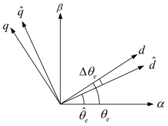
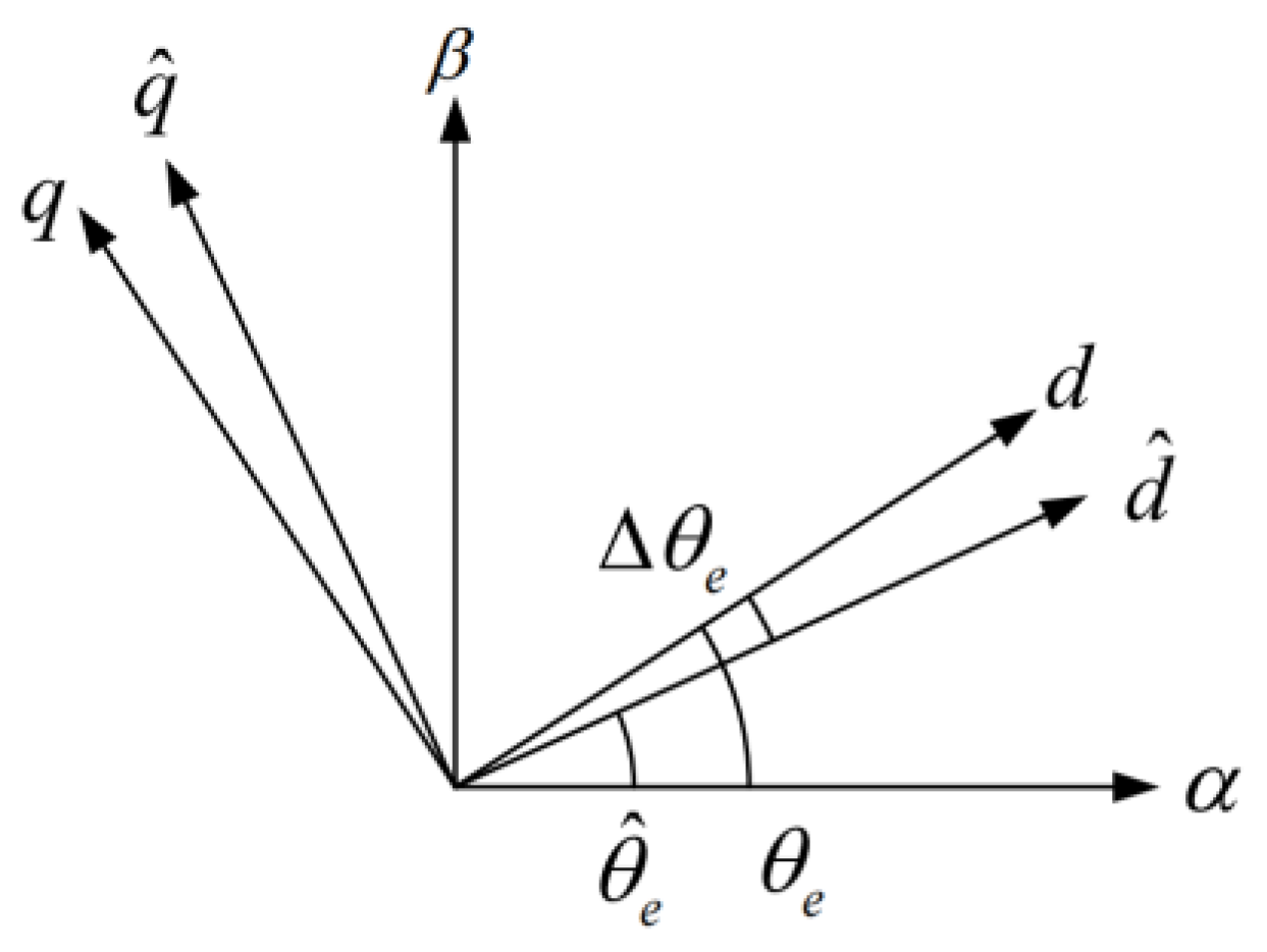
The pulsating voltage is injected along the d-axis of the estimated synchronous frame. The relationship among the reference frames is shown in Figure 1, where ${\theta }_e$ is the actual rotor position, ${\widehat{\theta }}_{\mathrm{e}}$ is the estimated position, and $\mathrm{\Delta }{\theta }_{\mathrm{e}}$ is the position error.

Figure 1. Relationship among the actual, estimated, and stationary reference frames.

When the estimated and actual reference frames are not aligned, the stationary-frame high-frequency current contains information on the angular error. Demodulation of this current yields a position-error signal, which is regulated to zero by a PLL or a position-tracking loop.

The voltage transformation between the actual and estimated frames is

$$\left[\begin{array}{c}{u}_{\mathrm{dh}}\\ u_{\mathrm{qh}}\end{array}\right]=R(\mathrm{\Delta }{\theta }_{\mathrm{e}})\left[\begin{array}{c}{u}_{\hat{\mathrm{d}}\mathrm{h}}\\ u_{\hat{\mathrm{q}}\mathrm{h}}\end{array}\right]$$

(5)

where

$$R(\mathrm{\Delta }{\theta }_{\mathrm{e}})=\left[\begin{array}{cc}\cos \mathrm{\Delta }{\theta }_{\mathrm{e}}& \sin \mathrm{\Delta }{\theta }_{\mathrm{e}}\\ -\sin \mathrm{\Delta }{\theta }_{\mathrm{e}}& \cos \mathrm{\Delta }{\theta }_{\mathrm{e}}\end{array}\right]$$

(6)

The injected voltage is applied along the estimated d-axis, and the rotor position is reconstructed in the stationary frame. The symbol u_inj denotes the injected high-frequency voltage.

$$\left[\begin{array}{c}{u}_{\hat{\mathrm{d}}\mathrm{h}}\\ u_{\hat{\mathrm{q}}\mathrm{h}}\end{array}\right]=\left[\begin{array}{c}{u}_{\mathrm{inj}}\\ 0\end{array}\right]$$

(7)

The high-frequency current components in the stationary frame are extracted as

$$\left[\begin{array}{c}{i}_{\mathrm{\alpha }\mathrm{h}}\\ i_{\mathrm{\beta }\mathrm{h}}\end{array}\right]=\left[\begin{array}{c}{\displaystyle \frac{\cos {\theta }_{\mathrm{e}}\cos \mathrm{\Delta }{\theta }_{\mathrm{e}}}{L_{dh}}}+{\displaystyle \frac{\sin {\theta }_{\mathrm{e}}\sin \mathrm{\Delta }{\theta }_{\mathrm{e}}}{L_{qh}}}\\ {\displaystyle \frac{\sin {\theta }_{\mathrm{e}}\cos \mathrm{\Delta }{\theta }_{\mathrm{e}}}{L_{\mathrm{dh}}}}-{\displaystyle \frac{\cos {\theta }_{\mathrm{e}}\sin \mathrm{\Delta }{\theta }_{\mathrm{e}}}{L_{\mathrm{qh}}}}\end{array}\right]\int u_{\mathrm{inj}}\mathrm{d}t$$

(8)

where i_αh and i_βh denote the stationary-frame high-frequency current components.

These components can be obtained using a high-pass filter or a filterless algebraic method.

$$\left[\begin{array}{c}{i}_{\mathrm{\alpha }\mathrm{h}}\\ i_{\mathrm{\beta }\mathrm{h}}\end{array}\right]=\mathrm{HPF}\left(\left[\begin{array}{c}{i}_{\mathrm{\alpha }}\\ i_{\mathrm{\beta }}\end{array}\right]\right)$$

(9)

where i_α and i_β are the stationary-frame stator currents, and HPF{·} denotes the high-pass-filtering operation.

The α- and β-axis current increments are calculated from two consecutive high-frequency current samples:

$$\left[\begin{array}{c}\mathrm{\Delta }{i}_{\mathrm{\alpha }\mathrm{h}}[k]\\ \mathrm{\Delta }{i}_{\mathrm{\beta }\mathrm{h}}[k]\end{array}\right]=\left[\begin{array}{c}{i}_{\mathrm{\alpha }\mathrm{h}}[k]\\ i_{\mathrm{\beta }\mathrm{h}}[k]\end{array}\right]-\left[\begin{array}{c}{i}_{\mathrm{\alpha }\mathrm{h}}[k-1]\\ i_{\mathrm{\beta }\mathrm{h}}[k-1]\end{array}\right]$$

(10)

where k is the discrete-time sample index, and Δi_αh [k] and Δi_βh [k] are the differences between two consecutive high-frequency current samples.

Compensation for the polarity of the injected voltage gives two orthogonal signals containing the rotor-position information.

$$\begin{array}{l}\mathrm{\Delta }{i}_{\cos }=\mathrm{sign}(u_{\mathrm{inj}})\cdot \mathrm{\Delta }{i}_{\mathrm{\alpha }\mathrm{h}}[k]\\ \mathrm{\Delta }{i}_{\sin }=\mathrm{sign}(u_{\mathrm{inj}})\cdot \mathrm{\Delta }{i}_{\mathrm{\beta }\mathrm{h}}[k]\end{array}$$

(11)

Here, Δi_cos and Δi_sin are the polarity-compensated orthogonal current increments.

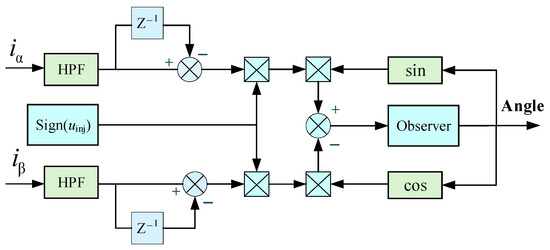
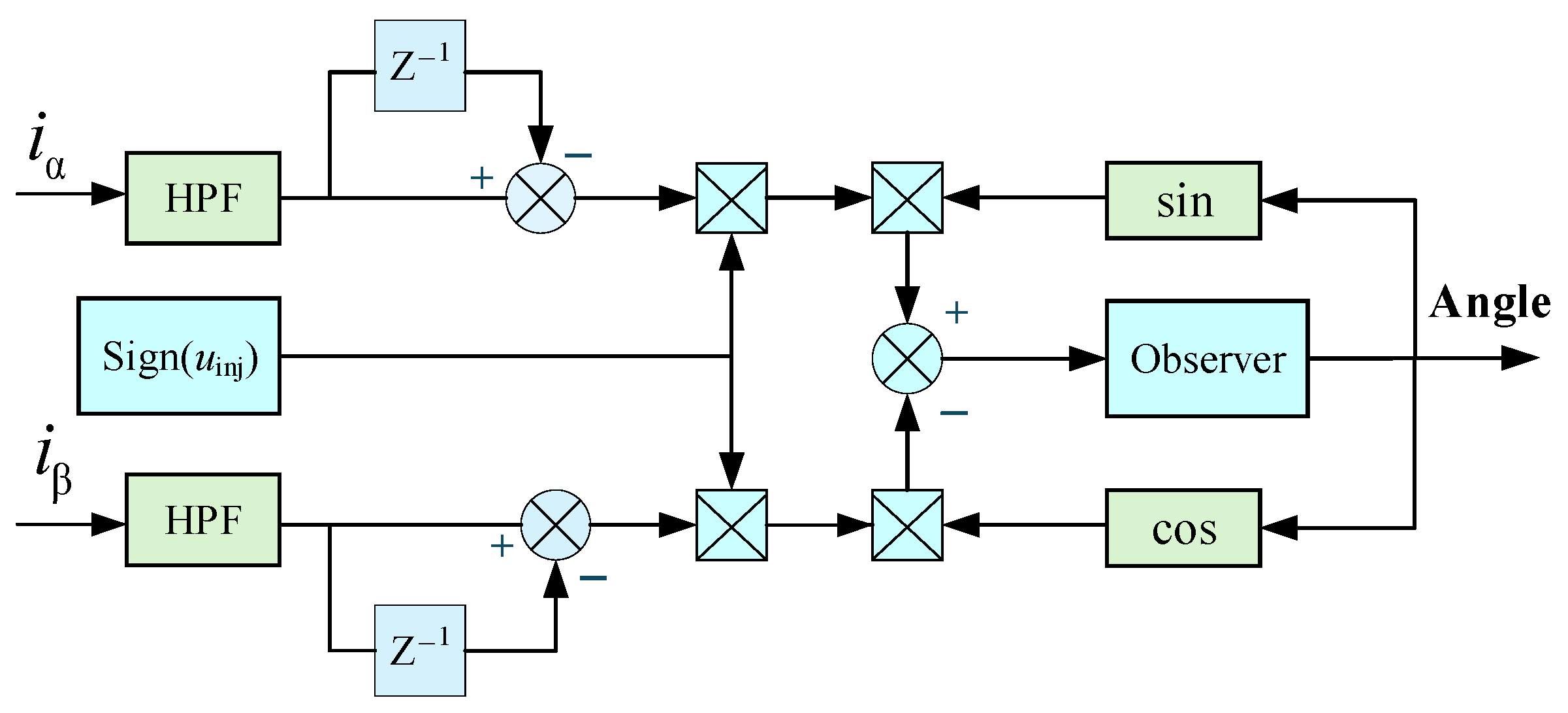
The orthogonal signals are low-pass filtered to attenuate switching components. Heterodyne demodulation is then used to obtain the equivalent position-error signal, as shown in Figure 2.

$$\mathsf{\epsilon }=\sin {\widehat{\theta }}_{\mathrm{e}}\cdot \mathrm{\Delta }{i}_{\cos }-\cos {\widehat{\theta }}_{\mathrm{e}}\cdot \mathrm{\Delta }{i}_{\sin }$$

(12)

where ε is the demodulated HFI position-error signal.

Figure 2. HFI demodulation structure. HPF denotes the high-pass filter, Z⁻¹ represents a one-sample delay, and Sign (u_inj) denotes the polarity of the injected voltage.

Closing the position-tracking loop forces the error signal to zero and aligns the estimated reference frame with the rotor reference frame.

The demodulated error is processed by a PLL or position-tracking loop. The resulting HFI position estimate, denoted by ${\widehat{\theta }}_{\mathrm{hfi}}$, is used for low-speed feedback and as the synchronization reference for the active flux observer.

3. Active Flux Observer for Medium- and High-Speed Sensorless Control

At medium and high speeds, the rotor position is estimated from the fundamental stator voltage and current. The unequal dq-axis inductances of an IPMSM must be included in the observer model. Accordingly, the stator flux is selected as the observer state, and the active flux vector is extracted from it to represent the rotor-position-related flux component.

3.1. State-Space Model in the Stationary αβ Frame

After applying the Clarke transformation, the stator voltage and flux equations in the stationary αβ frame are written as

$$\left[\begin{array}{c}{u}_{\mathrm{\alpha }}\\ u_{\mathrm{\beta }}\end{array}\right]=\left[\begin{array}{cc}R& 0\\ 0& R\end{array}\right]\left[\begin{array}{c}{i}_{\mathrm{\alpha }}\\ i_{\mathrm{\beta }}\end{array}\right]+{\displaystyle \frac{\mathrm{d}}{\mathrm{d}t}}\left[\begin{array}{c}{\psi }_{\mathrm{s}\mathrm{\alpha }}\\ {\psi }_{\mathrm{s}\mathrm{\beta }}\end{array}\right]$$

(13)

where u_α and u_β are the α- and β-axis stator voltages (V). The variables i_α and i_β are the corresponding stator currents (A), while ψ_sα and ψ_sβ are the stator flux linkages (Wb). The symbol R denotes the stator resistance (Ω).

The active-flux magnitude is defined as:

$${\psi }_{\mathrm{e}}={\psi }_{\mathrm{f}}+\left(L_{\mathrm{d}}-L_{\mathrm{q}}\right)i_{\mathrm{d}}$$

(14)

For observer design, the state vector is chosen as the stationary-frame stator-flux vector, i.e., x₁ = ψ_sα and x₂ = ψ_sβ

$$\mathit{x}=\left[\begin{array}{c}{x}_1\\ x_2\end{array}\right]=\left[\begin{array}{cc}{L}_{\mathrm{q}}& 0\\ 0& L_{\mathrm{q}}\end{array}\right]\left[\begin{array}{c}{i}_{\mathrm{\alpha }}\\ i_{\mathrm{\beta }}\end{array}\right]+{\psi }_{\mathrm{e}}\left[\begin{array}{c}\cos {\theta }_{\mathrm{e}}\\ \sin {\theta }_{\mathrm{e}}\end{array}\right]$$

(15)

It follows from (15) that the rotor-position information is contained in the active flux vector rather than in the permanent-magnet flux alone.

The input term for the flux observer is defined as

$$\mathit{y}=-\left[\begin{array}{cc}R& 0\\ 0& R\end{array}\right]\left[\begin{array}{c}{i}_{\mathrm{\alpha }}\\ i_{\mathrm{\beta }}\end{array}\right]+\left[\begin{array}{c}{u}_{\mathrm{\alpha }}\\ u_{\mathrm{\beta }}\end{array}\right]$$

(16)

The nominal state equation is therefore

$$\stackrel{·}{\mathit{x}}=\mathit{y}$$

(17)

Although direct integration of (17) yields the stator flux in principle, voltage offsets, measurement noise, and initial-condition errors cause drift in a digital implementation. A nonlinear correction based on the active flux magnitude is therefore introduced.

3.2. Nonlinear Active Flux Observer

Since the observer state is selected as the stator-flux vector, i.e., x = ψ_sαβ, subtracting the q-axis inductive flux from x gives the active-flux vector aligned with the rotor magnetic axis. Define

$$\eta (x)=\mathit{x}-\left[\begin{array}{cc}{L}_{\mathrm{q}}& 0\\ 0& L_{\mathrm{q}}\end{array}\right]\left[\begin{array}{c}{i}_{\mathrm{\alpha }}\\ i_{\mathrm{\beta }}\end{array}\right]$$

(18)

The vector η(x) represents the active flux, and its magnitude satisfies

$$\Vert \eta (x){\Vert }_2^2={\psi }_{\mathrm{e}}^2$$

(19)

where ‖·‖² denotes the Euclidean norm.

Under the adopted i_d = 0 control, the active flux magnitude reduces to

$${\psi }_{\mathrm{e}}={\psi }_{\mathrm{f}}$$

(20)

Following the nonlinear flux-observer framework reported in [28], the constant-magnitude property of the active-flux vector is used to construct the nonlinear correction term. Accordingly, the nonlinear observer is formulated as

$$\dot{\widehat{x}}=y+{\displaystyle \frac{\gamma }{2}}\eta (\widehat{x})\left[{\psi }_{\mathrm{e}}^2-\Vert \eta (\widehat{x}){\Vert }^2\right]$$

(21)

where $\widehat{x}$ is the estimated state vector and γ is the observer feedback gain.

The nonlinear feedback term in (21) forces the estimated active flux toward its nominal magnitude. It therefore mitigates the drift associated with pure voltage-model integration and reduces the sensitivity of the flux estimate to moderate parameter errors.

3.3. Rotor Position and Speed Estimation

The estimated active-flux vector is then computed as

$${\widehat{\psi }}_{\mathrm{e}}=\widehat{x}-L_{\mathrm{q}}\left[\begin{array}{c}{i}_{\mathrm{\alpha }}\\ i_{\mathrm{\beta }}\end{array}\right]$$

(22)

Its stationary-frame components are

$${\widehat{\psi }}_{\mathrm{e}}=\left[\begin{array}{c}{\widehat{\psi }}_{\mathrm{e}\mathrm{\alpha }}\\ {\widehat{\psi }}_{\mathrm{e}\mathrm{\beta }}\end{array}\right]$$

(23)

The rotor position can be extracted from the estimated active-flux vector using either direct arctangent calculation or a phase-locked loop. The direct calculation is expressed as

$${\widehat{\theta }}_{obs}=\mathrm{atan}2\left({\widehat{\psi }}_{\mathrm{e}\mathrm{\beta }},{\widehat{\psi }}_{\mathrm{e}\mathrm{\alpha }}\right)$$

(24)

Alternatively, a PLL can be employed to obtain filtered position and speed estimates directly from the estimated active-flux components. Its phase-detector error is defined as

$$\mathrm{\Delta }\epsilon =-{\widehat{\psi }}_{\mathrm{e}\mathrm{\alpha }}\sin {\widehat{\theta }}_{\mathrm{o}\mathrm{b}\mathrm{s}}+{\widehat{\psi }}_{\mathrm{e}\mathrm{\beta }}\cos {\widehat{\theta }}_{\mathrm{o}\mathrm{b}\mathrm{s}}$$

(25)

The phase error is processed by a PI regulator to obtain the electrical speed estimate. Integration of this estimate yields the position ${\widehat{\theta }}_{\mathrm{o}\mathrm{b}\mathrm{s}}$ used by the current controller.

4. Wide-Speed-Range Control with Observer Pre-Synchronization and Sigmoid-Based Transition

The HFI estimator and the active flux observer exhibit different estimation dynamics. A direct transition between them can therefore introduce an abrupt change in the feedback angle, which disturbs the current-vector orientation and may induce current and torque transients. The proposed control scheme uses a finite transition region, observer pre-synchronization, and vector-domain angle blending.

4.1. Operating-Region Definition

The speed range is divided into a low-speed region, a transition region, and a medium- and high-speed region. The boundaries are denoted by n_low and n_high. A finite transition region also prevents repeated switching when the speed oscillates around a single threshold.

The lower boundary n_low is selected above the minimum speed at which the active flux observer provides a reliable estimate. Below this boundary, the weak back-EMF and inverter nonlinearities limit model-based estimation; hence, the feedback angle is supplied entirely by the HFI estimator.

The upper boundary n_high is selected according to the required transition time and the voltage margin occupied by the injected signal. Above this boundary, HFI is disabled and the active flux observer supplies the position and speed estimates. Within the transition region, both estimators remain active and their outputs are blended.

4.2. Pre-Synchronization of the Active Flux Observer

Before angle blending is initiated, the active flux observer must be aligned with the HFI estimate. When the observer runs in the background at low speed, the small back-EMF, inverter nonlinearities, and measurement noise may produce a substantial phase error. The following pre-synchronization law corrects this error before the drive enters the transition region.

In the low-speed region, the HFI angle ${\widehat{\theta }}_{\mathrm{hfi}}$ defines the reference active flux vector ${\psi }_{\mathrm{ref}}$. The active flux estimated by the observer is denoted by ${\widehat{\psi }}_{\mathrm{e}\mathrm{\Sigma }}$. In the stationary frame, these vectors are expressed as

$${\psi }_{\mathrm{ref}}={\psi }_{\mathrm{f}}\left[\begin{array}{c}\cos {\widehat{\theta }}_{\mathrm{hfi}}\\ \sin {\widehat{\theta }}_{\mathrm{hfi}}\end{array}\right]$$

(26)

$${\widehat{\psi }}_{\mathrm{e}}={\psi }_{\mathrm{f}}\left[\begin{array}{c}\cos {\widehat{\theta }}_{\mathrm{obs}}\\ \sin {\widehat{\theta }}_{\mathrm{obs}}\end{array}\right]$$

(27)

The wrapped phase error between the HFI estimator and the active flux observer is defined as

$$\mathrm{\Delta }\theta =\mathrm{atan}2\left(\sin \left({\widehat{\theta }}_{\mathrm{hfi}}-{\widehat{\theta }}_{\mathrm{obs}}\right),\cos \left({\widehat{\theta }}_{\mathrm{hfi}}-{\widehat{\theta }}_{\mathrm{obs}}\right)\right)$$

(28)

Linearizing the reference active flux vector around the current observer angle gives

$${\psi }_{\mathrm{ref}}={\psi }_{\mathrm{f}}\left[\begin{array}{c}\cos ({\widehat{\theta }}_{\mathrm{obs}}+\mathrm{\Delta }\theta )\\ \sin ({\widehat{\theta }}_{\mathrm{obs}}+\mathrm{\Delta }\theta )\end{array}\right]={\psi }_{\mathrm{f}}\left[\begin{array}{c}\cos {\widehat{\theta }}_{\mathrm{obs}}\cos \mathrm{\Delta }\theta -\sin {\widehat{\theta }}_{\mathrm{obs}}\sin \mathrm{\Delta }\theta \\ \sin {\widehat{\theta }}_{\mathrm{obs}}\cos \mathrm{\Delta }\theta +\cos {\widehat{\theta }}_{\mathrm{obs}}\sin \mathrm{\Delta }\theta \end{array}\right]$$

(29)

For a sufficiently small phase error, the first-order approximation gives

$$\cos \mathrm{\Delta }\theta \approx 1,\sin \mathrm{\Delta }\theta \approx \mathrm{\Delta }\theta$$

(30)

Substituting (30) into (29) yields

$${\psi }_{\mathrm{ref}}\approx {\psi }_{\mathrm{f}}\left[\begin{array}{c}\cos {\widehat{\theta }}_{\mathrm{obs}}\\ \sin {\widehat{\theta }}_{\mathrm{obs}}\end{array}\right]+\mathrm{\Delta }\theta \cdot {\psi }_{\mathrm{f}}\left[\begin{array}{c}-\sin {\widehat{\theta }}_{\mathrm{obs}}\\ \cos {\widehat{\theta }}_{\mathrm{obs}}\end{array}\right]={\widehat{\psi }}_{\mathrm{f}}+\mathrm{\Delta }\theta \cdot \left[\begin{array}{cc}0& -1\\ 1& 0\end{array}\right]{\widehat{\psi }}_{\mathrm{f}}$$

(31)

Define the 90° rotation matrix as

$$J=\left[\begin{array}{cc}0& -1\\ 1& 0\end{array}\right]$$

(32)

Hence, to first order, the difference between the reference and estimated active flux vectors is a tangential component orthogonal to the estimated flux vector:

$${\psi }_{\mathrm{ref}}-{\widehat{\psi }}_{\mathrm{f}}\approx \mathrm{\Delta }\theta \cdot \mathit{J}{\widehat{\psi }}_{\mathrm{f}}$$

(33)

This relationship motivates an orthogonal correction term in the observer dynamics, which directly compensates the phase error.

Define the integral state $\dot{\xi }$ as

$$\dot{\xi }=\mathrm{\Delta }\theta$$

(34)

A proportional-integral synchronization signal is generated as

$$u_{\mathrm{sync}}=K_{\mathrm{ps}}\mathrm{\Delta }\theta +K_{\mathrm{is}}\xi$$

(35)

where K_ps and K_is are the proportional and integral gains of the pre-synchronization controller, respectively.

In the digital implementation, the synchronization PI output is limited to the prescribed correction range, and a back-calculation anti-windup mechanism is applied by feeding the saturation error back to the integral state.

The corresponding orthogonal correction term is

$$U_{\mathrm{sync}}=W_{\mathrm{hfi}}{u}_{\mathrm{sync}}J{\widehat{\psi }}_{\mathrm{e}}=W_{\mathrm{hfi}}(K_{\mathrm{ps}}\mathrm{\Delta }\theta +K_{\mathrm{is}}\xi )J{\widehat{\psi }}_{\mathrm{e}}$$

(36)

where W_hfi is the current HFI weighting factor, and U_sync is the two-axis correction vector added to the observer-state dynamics.

Adding (36) to the observer in (21) gives the pre-synchronized observer dynamics.

$$\dot{\widehat{x}}=y+{\displaystyle \frac{\gamma }{2}}\eta (\widehat{x})\left[{\psi }_{\mathrm{e}}^2-\Vert \eta (\widehat{x}){\Vert }_2^2\right]+W_{\mathrm{hfi}}(K_{\mathrm{ps}}\mathrm{\Delta }\theta +K_{\mathrm{is}}\xi )J{\widehat{\psi }}_{\mathrm{e}}$$

(37)

Under the small-angle approximation used in (29)–(33), the local synchronization-error dynamics can be written as d(e_θ)/dt = −g_s(K_ps e_θ + K_is ξ) and dξ/dt = e_θ, where g_s > 0 denotes the effective gain of the orthogonal state correction. Consider the Lyapunov function V = e_θ²/2 + g_s K_is ξ²/2. For K_ps > 0 and K_is > 0, its derivative satisfies dV/dt = −g_s K_ps e_θ² ≤ 0. The largest invariant set satisfying dV/dt = 0 is e_θ = ξ = 0; therefore, the local synchronization-error dynamics are asymptotically stable.

The correction is active in the low-speed region and drives the observer angle toward the HFI angle before the transition. Its contribution is reduced together with the HFI weight during the subsequent blending process.

4.3. Sigmoid-Based Smooth Transition

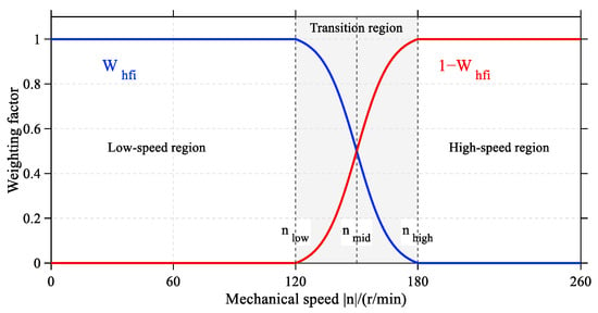
After pre-synchronization, the estimator outputs and the injected voltage are transferred continuously over the transition region. A sigmoid function is adopted to generate the HFI weighting factor.

The HFI weighting factor W_hfi is defined as

$$\begin{array}{l}{W}_{\mathrm{hfi}}(|n|)=\left\{\begin{array}{ll}1,\hfill & |n|\le n_{\mathrm{low}},\hfill \\ {\displaystyle \frac{S(|n|)-S_{\mathrm{high}}}{S_{\mathrm{low}}-S_{\mathrm{high}}}},\hfill & n_{\mathrm{low}}<|n|<n_{\mathrm{high}},\hfill \\ 0,\hfill & \left|n\right|\ge n_{\mathrm{high}}.\hfill \end{array}\right.\\ S(|n|)={\displaystyle \frac{1}{1+\exp \left[\lambda \left(\left|n\right|-n_{\mathrm{mid}}\right)\right]}}{S}_{\mathrm{low}}=S\left(n_{\mathrm{low}}\right),S_{\mathrm{high}}=S\left(n_{\mathrm{high}}\right)\end{array}$$

(38)

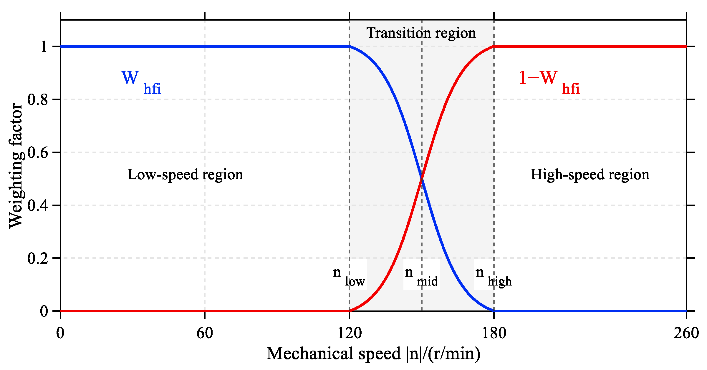
where n is the per-unit mechanical speed normalized by a base speed of 1200 r/min, and λ is a dimensionless slope coefficient. In this study, n_low = 0.10, n_mid = 0.125, n_high = 0.15, and λ = 200. Therefore, λ(n_mid − n_low) = λ(n_high − n_mid) = 5, producing a slow–fast–slow weight-transfer profile. The boundary normalization guarantees W_hfi(n_low) = 1 and W_hfi(n_high) = 0; hence, Equation (38) is continuous at both transition boundaries. The corresponding weighting profiles are shown in Figure 3.

Figure 3. Sigmoid weighting for angle blending and HFI voltage scaling.

Because the rotor angle is periodic, direct scalar interpolation may cause a wraparound discontinuity. The HFI and observer angles are therefore mapped onto unit vectors and blended using W_hfi:

$$\left[\begin{array}{c}{p}_{\mathrm{sync}\_\mathrm{\alpha }}\\ p_{\mathrm{sync}\_\mathrm{\beta }}\end{array}\right]=W_{\mathrm{hfi}}\left[\begin{array}{c}\cos {\widehat{\theta }}_{\mathrm{hfi}}\\ \sin {\widehat{\theta }}_{\mathrm{hfi}}\end{array}\right]+(1-W_{\mathrm{hfi}})\left[\begin{array}{c}\cos {\widehat{\theta }}_{\mathrm{obs}}\\ \sin {\widehat{\theta }}_{\mathrm{obs}}\end{array}\right]$$

(39)

where p_{sync_α} and p_{sync_β} are the α- and β-axis components of the blended unit position vector, respectively.

The blended rotor position used by the current controller is then obtained from

$${\widehat{\theta }}_{\mathrm{final}}=\mathrm{atan}2\left(p_{\mathrm{sync}\_\mathrm{\beta }},p_{\mathrm{sync}\_\mathrm{\alpha }}\right)$$

(40)

The same weighting factor scales the injected voltage. The commanded HFI amplitude is

$$U_{\mathrm{inj}}^{\ast }(|n|)=W_{\mathrm{hfi}}(|n|)\cdot U_{\mathrm{inj}0}$$

(41)

where U_inj0 is the preset HFI voltage amplitude in the low-speed region (V).

The same weighting factor is applied to both the estimator blending and the injected-voltage amplitude. Therefore, as the HFI voltage and the resulting high-frequency current component are gradually attenuated, the contribution of the HFI estimator to the fused position is reduced simultaneously, while the active-flux observer becomes dominant. The fundamental dq-axis current references and current-control structure remain unchanged during this process. Consequently, the progressive voltage scaling avoids an abrupt high-frequency current disturbance without relying on the weakened HFI response near the upper transition boundary.

During acceleration, W_hfi decreases continuously from unity to zero. Consequently, the HFI contribution to the blended angle and the injected voltage amplitude decrease simultaneously, and the position feedback is supplied only by the active flux observer above n_high. During deceleration, the sequence is reversed and the HFI voltage is restored continuously.

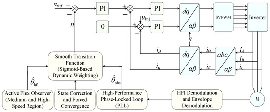
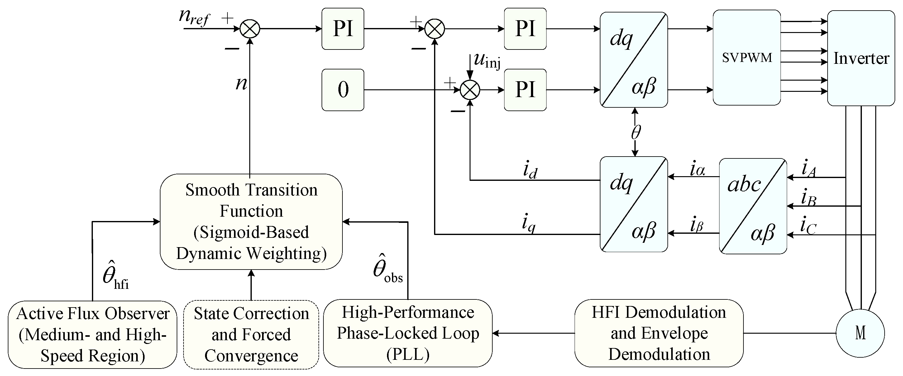
The overall block diagram of the proposed control system, including the HFI estimator, active-flux observer, observer pre-synchronization, sigmoid-based weighting, HFI voltage scaling, and current control loop, is shown in Figure 4.

Figure 4. Overall block diagram of the proposed wide-speed-range sensorless control system. PI denotes the proportional–integral controller, PLL denotes the phase-locked loop, HFI denotes high-frequency injection, and SVPWM denotes space-vector pulse-width modulation.

5. Experimental Results

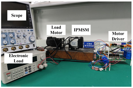
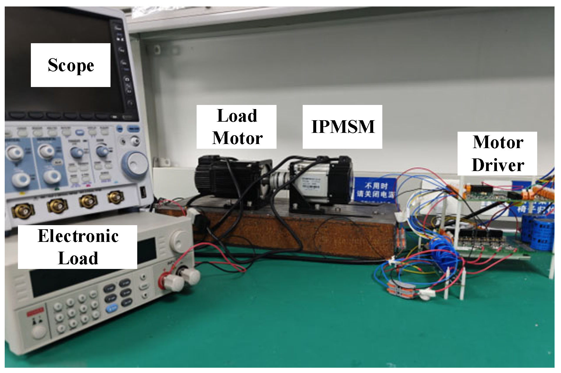
The proposed method was evaluated on the 0.4-kW IPMSM drive shown in Figure 5. The setup consists of the test motor, a power converter, a digital controller, a host computer, and a loading machine. The control algorithm was implemented in real time on a TMS320F28075 digital signal processor (Texas Instruments, Dallas, TX, USA). The inverter was supplied by a 70 V dc link and operated at a PWM switching frequency of 10 kHz. The stator currents were measured using CASR-6 current sensors (LEM International SA, Meyrin, Switzerland) and sampled at 10 kHz, and the current-control algorithm was also updated at 10 kHz. A shaft-mounted 2000-line encoder was used only to provide the reference rotor position for experimental evaluation and was not involved in the sensorless control loop. The loading machine was mechanically coupled to the tested IPMSM and operated as a generator. Its output was connected to an electronic load operating in constant-current mode, so that load disturbances could be applied by changing the electronic-load current. The motor parameters and the main digital control parameters are listed in Table 1 and Table 2, respectively. The experimental tests covered low-speed HFI estimation, medium- and high-speed active flux estimation, observer pre-synchronization, and the transition between the two estimation methods.

Figure 5. Experimental setup.

Table 1. IPMSM parameters.

Parameter	Value	Parameter	Value
Rated power	0.4 kW	Rated torque	1.06 N·m
Rated speed	3600 r/min	Stator resistance	3.69 Ω
Rated voltage	220 V	d-axis inductance	9.141 mH
Rated current	2.8 A	q-axis inductance	13.742 mH
Number of pole pairs	5	flux linkage	0.034 Wb

Table 2. Main digital control parameters.

Parameter	Value	Parameter	Value
Control frequency fctrl	10 kHz	Speed-loop frequency fω	1 kHz
Current-loop PI gains Kp,i, Ki,i	0.1, 0.0875	Speed-loop PI gains Kp,ω, Ki,ω	1.0, 0.01
HFI frequency fhfi	5 kHz	HFI tracking PI gains Kp,hfi, Ki,hfi	60, 2000
Observer gain γ	8.0 × 104	Pre-sync. PI gains Kps, Kis	60, 200
Transition speeds nlow, nmid, nhigh	120, 150, 180 r/min	Sigmoid coefficient λ	200

To ensure the reproducibility of the experimental results, the main controller gains and transition-related parameters used in the digital implementation are summarized in Table 2. The PI parameters listed in Table 2 are normalized discrete implementation coefficients used directly in the digital controller. In this digital control system, speed and current are represented in per-unit values, with base values of 1200 r/min and 30 A, respectively.

The amplitude of the injected high-frequency square-wave voltage was 20 V, corresponding to 0.5 p.u. in the adopted digital voltage normalization. The high- and low-frequency current components were separated using a carrier-based method rather than a conventional frequency-domain filter; therefore, this separation process does not require a filter cutoff frequency.

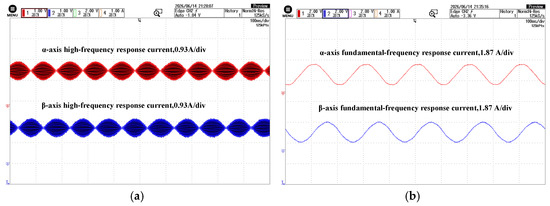
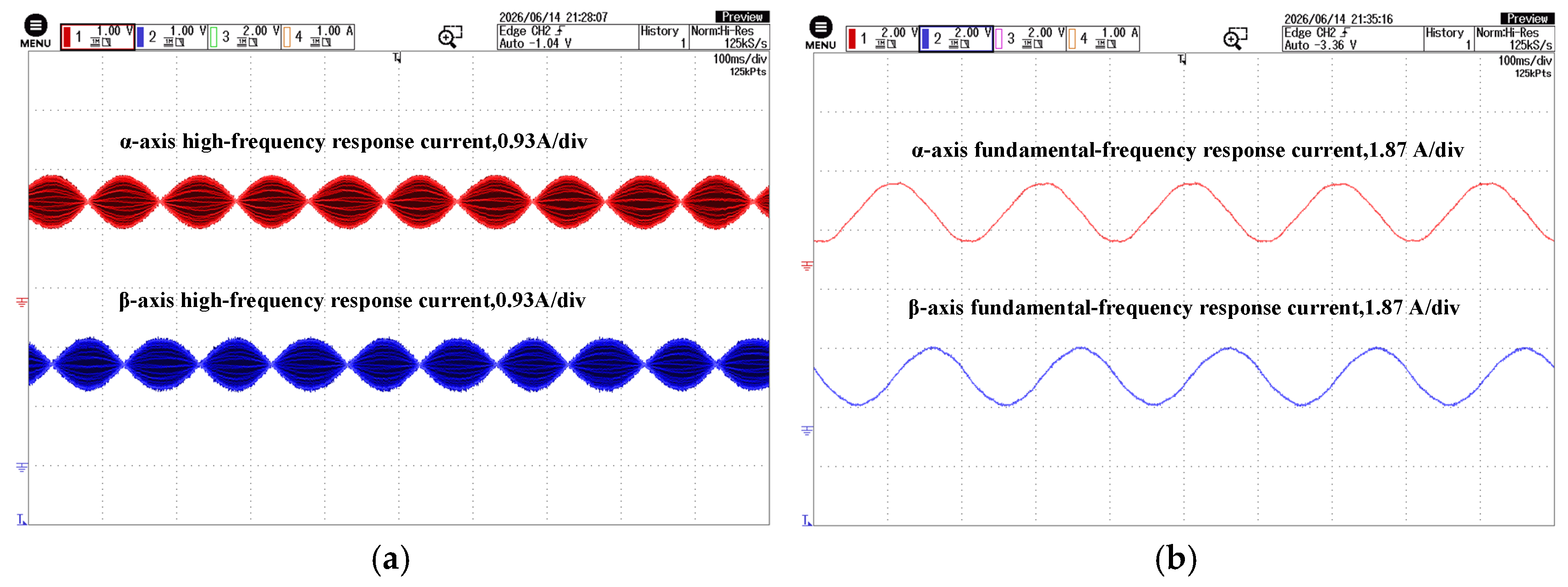
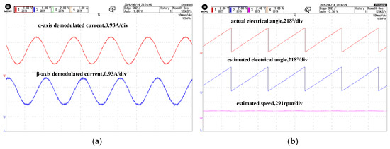
Figure 6 shows the current responses obtained in the low-speed HFI test at 60 r/min. The extracted α- and β-axis high-frequency response currents are shown in Figure 6a, while the corresponding fundamental-frequency current components are shown in Figure 6b.

Figure 6. Current waveforms under low-speed HFI. (a) High-frequency response current; (b) fundamental current.

As shown in Figure 6a, the injected high-frequency voltage produces clear high-frequency current components in the stationary frame. These components are separated from the fundamental-frequency current shown in Figure 6b, and therefore provide the saliency-dependent information required for HFI-based position estimation.

The demodulated HFI signals and the corresponding low-speed estimation results are shown in Figure 7.

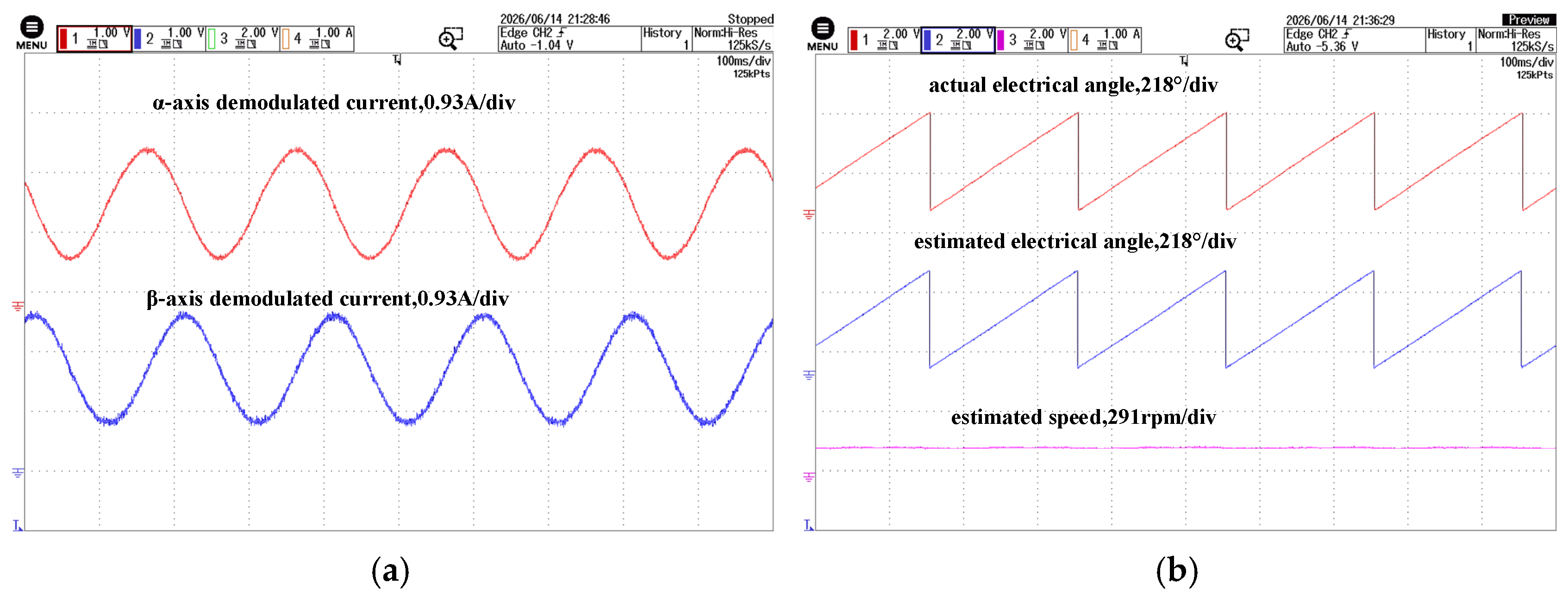
Figure 7. HFI demodulation and low-speed estimation results. (a) Demodulated signals; (b) estimated position and speed.

As shown in Figure 7a, the two demodulated components exhibit periodic characteristics and retain the rotor-position information after demodulation. In Figure 7b, the HFI-estimated angle closely follows the measured electrical angle, and the steady-state angle error is within 3°. The estimated speed remains stable at 60 r/min. These results confirm that the HFI estimator provides continuous position and speed feedback under the tested low-speed condition.

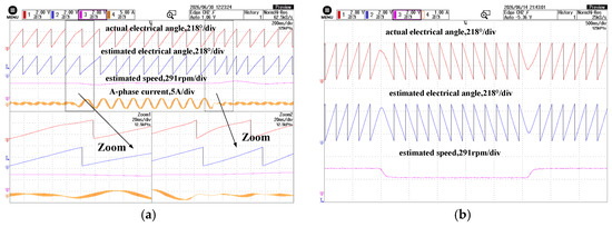
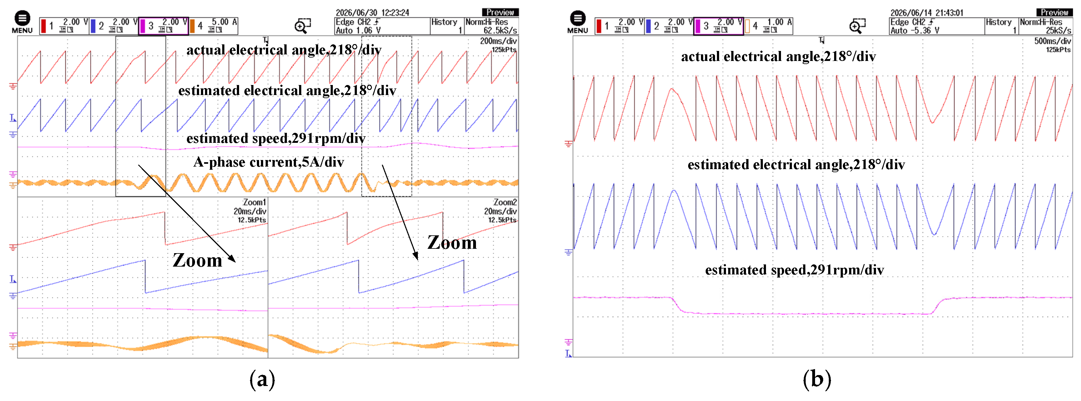
Figure 8 further evaluates the low-speed HFI estimator under load disturbance and forward/reverse transition.

Figure 8. Low-speed sensorless responses. (a) Load variation; (b) forward/reverse transition.

As shown in Figure 8a, a load disturbance is applied at 60 r/min by changing the electronic-load current from no load to 0.4 A in constant-current mode. After the load change, the HFI-estimated angle remains synchronized with the measured electrical angle, and no evident position jump or loss of tracking is observed. The estimated speed exhibits only a small transient variation and then returns to the steady value. Figure 8b shows the forward/reverse transition under HFI-based sensorless control. During the speed reversal between +60 r/min and −60 r/min, the estimated angle remains continuous, and the estimated speed changes smoothly with the command direction. These results indicate that the HFI estimator can maintain stable position feedback under the tested low-speed load disturbance and reversal conditions.

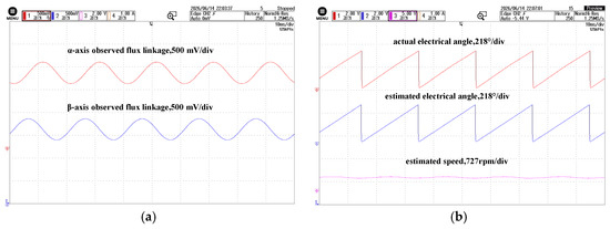
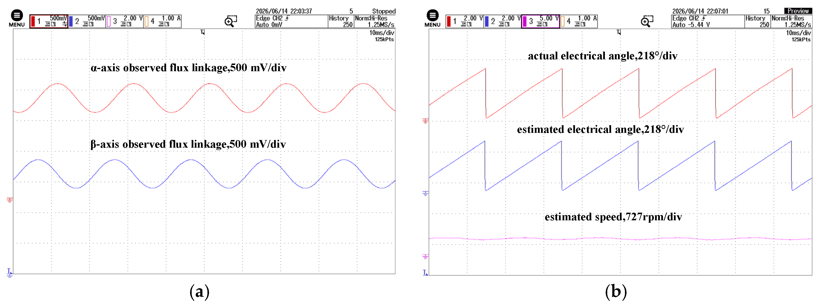
The medium-speed active-flux observer test was conducted at 600 r/min, and the results are shown in Figure 9.

Figure 9. Active flux observer results at 600 r/min. (a) Estimated active flux; (b) rotor position and speed estimation results.

As shown in Figure 9a, the estimated active-flux components form a continuous trajectory, from which the rotor-position information can be obtained. Figure 9b compares the measured electrical angle with the observer-estimated angle. The estimated angle follows the measured angle without observable divergence, and the steady-state angle error is within 3.5°. The estimated speed remains stable at 600 r/min. These results show that the active-flux observer can provide continuous position and speed feedback in the tested medium-speed region.

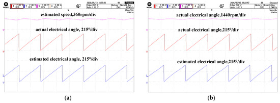
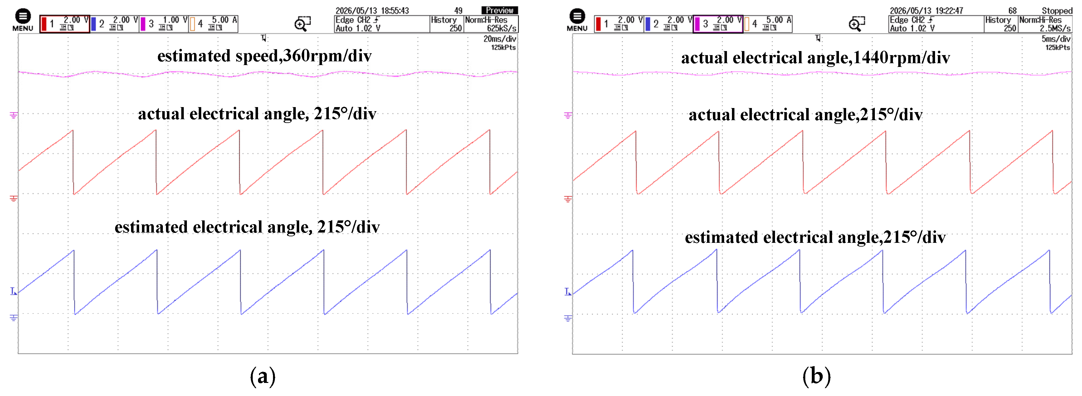
Figure 10 further evaluates the active-flux observer under parameter mismatch and field-weakening operation. In Figure 10a, an additional 1-Ω resistor was connected in series with phase A to emulate a stator-resistance mismatch. In Figure 10b, a negative d-axis current reference was applied to establish field-weakening operation at approximately 1440 r/min. Because the d-axis current is nonzero under this condition, the current-dependent inductive-flux component affects the position-observation model; therefore, the active-flux formulation developed in this paper was retained. In both tests, the estimated position tracks the encoder-referenced position, and the estimated speed remains stable without evident divergence or sustained oscillation. These results demonstrate robustness to stator-resistance mismatch and applicability under nonzero-id field-weakening operation.

Figure 10. Experimental results of the active-flux observer under parameter variation and field-weakening operation: (a) stator-resistance mismatch with an additional 1-Ω resistor connected in series with phase A; (b) field-weakening operation at approximately 1440 r/min with a negative d-axis current reference.

Figure 11 further verifies the active-flux observer under medium- and high-speed transient conditions.

Figure 11. Medium- and high-speed sensorless responses. (a) Load variation; (b) speed variation.

As shown in Figure 11a, a load disturbance is applied at 600 r/min by changing the electronic-load current from no load to 0.8 A in constant-current mode. After the load change, the observer-estimated angle remains aligned with the measured electrical angle, and no evident position jump or loss of tracking is observed. The estimated speed remains stable after a short transient response. Figure 11b shows the response during a 600–960–600 r/min speed variation with the electronic-load current maintained at 0.8 A. During the acceleration and deceleration processes, the observer-estimated angle continuously follows the measured electrical angle, and the estimated speed varies smoothly without observable oscillation or divergence. These results indicate that the active-flux observer can maintain continuous position and speed feedback under the tested medium- and high-speed load and speed variations.

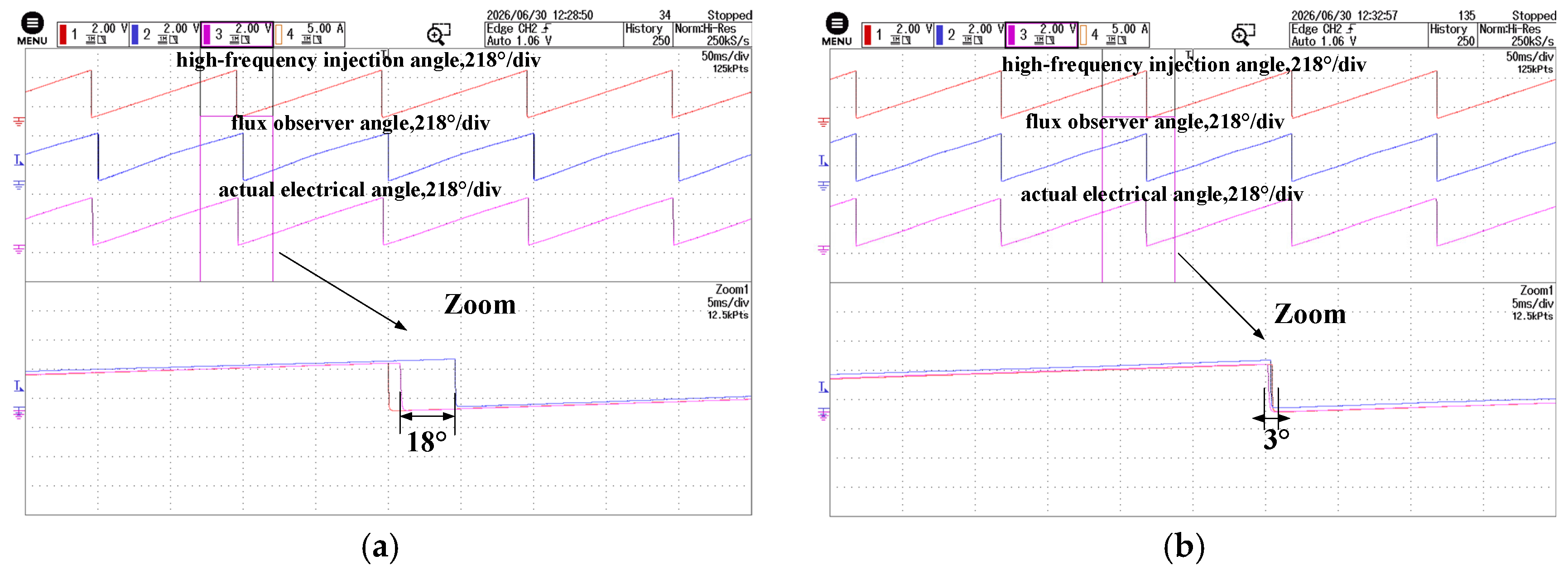
Observer pre-synchronization was evaluated at the lower boundary of the transition region, 120 r/min. Figure 12 compares the angular alignment between the HFI-estimated angle and the observer-estimated angle before and after pre-synchronization.

Figure 12. Active flux observer pre-synchronization at 120 r/min. (a) Without pre-synchronization; (b) with pre-synchronization.

As shown in Figure 12a, without pre-synchronization, an initial angular mismatch of approximately 18° exists between the HFI estimator and the active-flux observer. After pre-synchronization is enabled, this mismatch is reduced to approximately 3°, as shown in Figure 12b. This confirms that pre-synchronization aligns the observer state with the HFI estimate before angle blending.

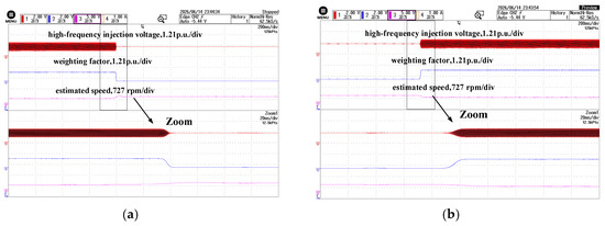
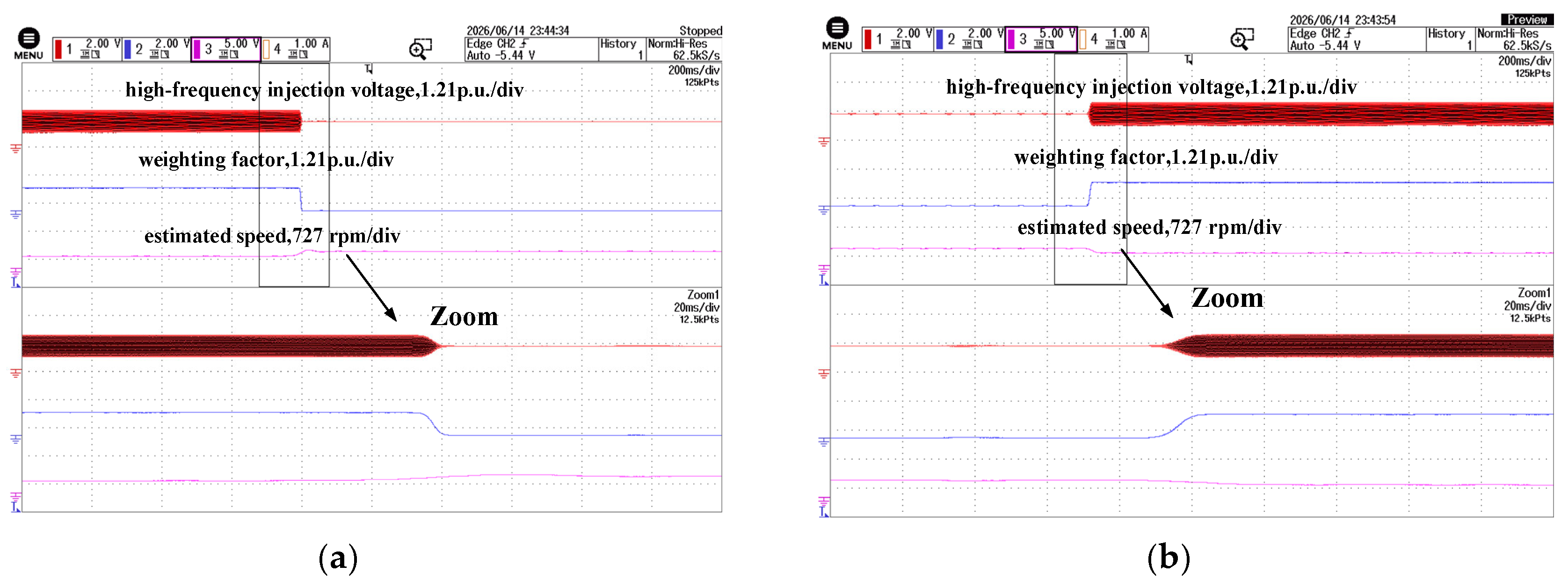
Figure 13 verifies the speed-dependent HFI voltage scaling during acceleration and deceleration through the 120–180 r/min transition region.

Figure 13. HFI voltage scaling over 120–180 r/min: (a) acceleration; (b) deceleration.

As shown in Figure 13a, when the speed increases from 120 r/min to 180 r/min, the HFI weighting factor decreases smoothly from 1 to 0. Accordingly, the HFI voltage command is reduced from 0.5 p.u. to 0 without an abrupt amplitude change. Figure 13b shows the reverse process during deceleration. When the speed decreases from 180 r/min to 120 r/min, the HFI weighting factor increases smoothly from 0 to 1, and the HFI voltage command is restored from 0 to 0.5 p.u. These results confirm that the HFI voltage is removed and restored continuously in coordination with the sigmoid weighting function.

The interval during which W_hfi changes between 1 and 0 directly represents the time spent in the 120–180 r/min transition region. From the enlarged waveforms in Figure 13, the measured transition durations are approximately 8 ms during acceleration and 12 ms during deceleration. The transition is governed by the instantaneous rotor speed rather than by a preset timing sequence; therefore, no fixed dwell time is required. However, an excessively rapid passage through the transition region may shorten the available time for estimator blending, so the transition width should be coordinated with the drive acceleration and the observer bandwidth.

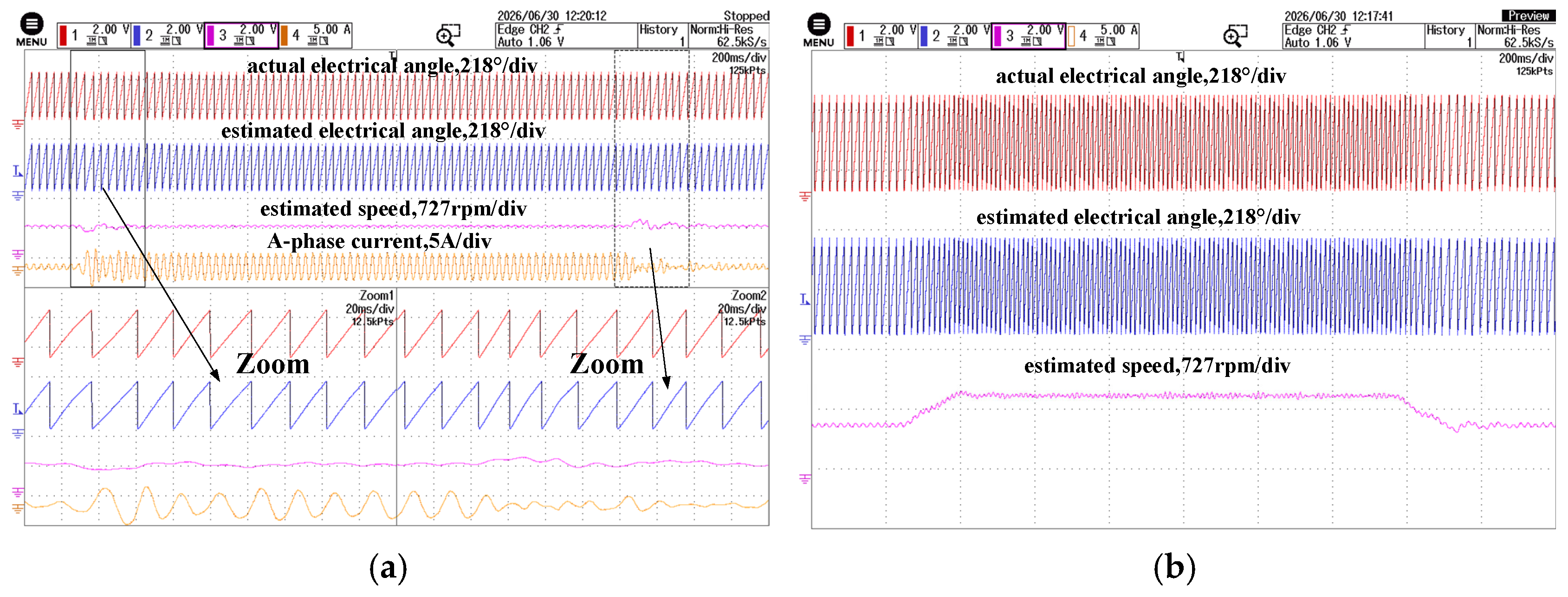
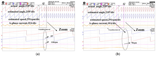
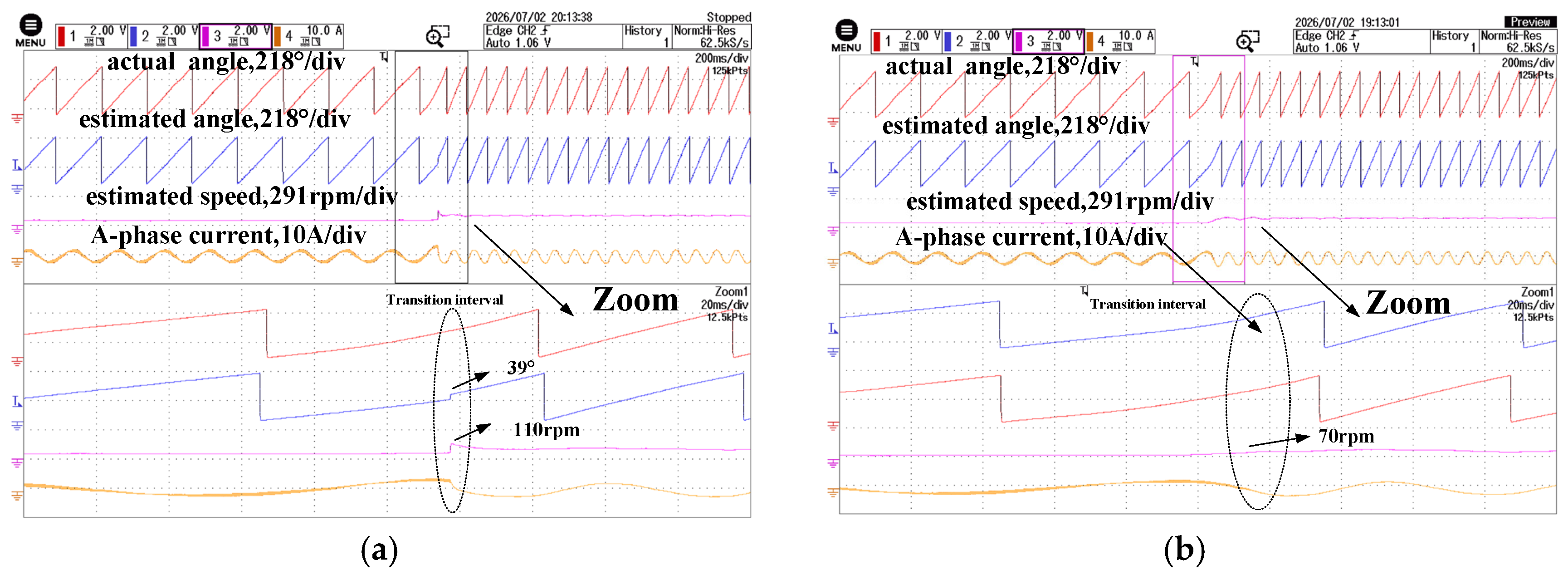
The transition performance is further evaluated by comparing the proposed method with a traditional weighted transition method, in which the HFI-estimated angle and the active-flux-observer angle are directly blended as scalar quantities using a linear speed-dependent weight, without observer pre-synchronization, as shown in Figure 14.

Figure 14. Acceleration transition responses under different transition methods. (a) Traditional weighted transition method; (b) proposed method.

As shown in Figure 14a, with the traditional weighted transition method, the initial angular mismatch between the two estimators can still be observed during the transition. In contrast, with the proposed method shown in Figure 14b, the active-flux observer is pre-synchronized before blending, and the final estimated angle maintains better continuity when passing through the 120–180 r/min transition region. The estimated speed also remains continuous, without an evident step change. These results indicate that observer pre-synchronization reduces the transition disturbance during acceleration.

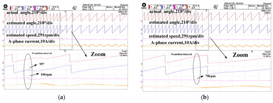
Figure 15 compares the deceleration transition from the active-flux-observer region back to the HFI region.

Figure 15. Deceleration transition responses under different transition methods. (a) Traditional weighted transition method; (b) proposed method.

As shown in Figure 14 and Figure 15, the conventional method produces estimated-angle steps of approximately 39° and 95° during acceleration and deceleration, respectively, whereas the proposed method achieves smooth angle transitions. Meanwhile, the maximum estimated-speed step is reduced from 110 to 70 r/min during acceleration and from 100 to 70 r/min during deceleration.

During deceleration, the sigmoid weighting function and vector-domain angle blending maintain continuous angle and speed estimation during the feedback-source change, as shown in Figure 15. Together with the acceleration results in Figure 14, this confirms smooth estimator transitions in both directions.

Overall, the experiments verify stable sensorless operation across the low-speed, transition, and medium- and high-speed regions. At 120 r/min, observer pre-synchronization reduces the angular mismatch between the two estimators from approximately 18° to 3°, while the sigmoid weighting function and vector-domain angle blending maintain continuous angle and speed estimation throughout the 120–180 r/min transition.

6. Conclusions

An observer pre-synchronization scheme has been proposed for the transition between the low-speed HFI estimator and the active-flux observer in an IPMSM sensorless drive. Before entering the transition region, the HFI-estimated angle is used to correct the state of the active-flux observer, thereby reducing the initial angular mismatch between the two estimators. A sigmoid weighting function is then used to blend the two angle vectors while scaling the injected voltage.

Experiments on a 0.4-kW IPMSM drive show that the proposed pre-synchronization reduces the angular mismatch between the HFI estimator and the active-flux observer from approximately 18° to 3° at 120 r/min. The present validation is limited to a 0.4-kW, 3600-r/min IPMSM, with the highest tested field-weakening speed being approximately 1440 r/min under the available 70-V dc-link and laboratory loading conditions; further validation closer to the rated speed and under broader parameter and load variations will be considered in future work.

References

- Wang, G.; Valla, M.I.; Solsona, J.A. Position sensorless permanent magnet synchronous machine drives—A review. IEEE Trans. Ind. Electron. 2020, 67, 5830–5842. [Google Scholar] [CrossRef] [Scilit]
- Zhang, Z. Sensorless back-EMF-based control of synchronous PM and reluctance motor drives—A review. IEEE Trans. Power Electron. 2022, 37, 10290–10305. [Google Scholar] [CrossRef] [Scilit]
- Zhu, P.; Zou, J.; Zhang, W.; Zhai, Y.; Zou, J.; Vazquez, S.; Franquelo, L.G.; Xu, Y. Improved resonant ESO-based sampling delay error suppression method for PMSM drives using a single dc-link current sensor. IEEE Trans. Ind. Electron. 2026, 73, 9692–9704. [Google Scholar] [CrossRef] [Scilit]
- Zhang, W.; Zhai, Y.; Zhu, P.; Xu, Y.; Zou, J.; Vazquez, S. Power regulated field-weakening control strategy with adaptive observers for permanent magnet synchronous motors. IEEE Trans. Transp. Electrif. 2026; early access. [CrossRef] [Scilit]
- Wang, Z.; Chang, S.; Vazquez, S.; Zhang, Z. Adjustable-order noise-resilient extended state observer for model-free predictive speed control. IEEE Trans. Ind. Electron. 2026; early access. [CrossRef] [Scilit]
- Ni, R.; Xu, D.; Blaabjerg, F.; Lu, K.; Wang, G.; Zhang, G. Square-wave voltage injection algorithm for PMSM position sensorless control with high robustness to voltage errors. IEEE Trans. Power Electron. 2017, 32, 5425–5437. [Google Scholar] [CrossRef] [Scilit]
- Hwang, C.-E.; Lee, Y.; Sul, S.-K. Analysis on position estimation error in position-sensorless operation of IPMSM using pulsating square wave signal injection. IEEE Trans. Ind. Appl. 2019, 55, 458–470. [Google Scholar] [CrossRef] [Scilit]
- Wu, T.; Zhu, H.; Wu, X.; Huang, S.; Yu, X.; Tan, Z.; Gao, F.; Tong, X. Enhanced sequential high-frequency voltage injection method for low-speed sensorless control of IPMSM. IEEE Trans. Power Electron. 2025, 40, 10836–10845. [Google Scholar] [CrossRef] [Scilit]
- Zhang, W.; Cheng, S.; Zhu, P.; Liu, Y.; Zou, J. Synchronized carrier-wave and high-frequency square-wave periodic modulation strategy for acoustic noise reduction in sensorless PMSM drives. Energies 2025, 18, 2729. [Google Scholar] [CrossRef] [Scilit]
- Kim, D.; Kwon, Y.-C.; Sul, S.-K.; Kim, J.-H.; Yu, R.-S. Suppression of injection voltage disturbance for high-frequency square-wave injection sensorless drive with regulation of induced high-frequency current ripple. IEEE Trans. Ind. Appl. 2016, 52, 302–312. [Google Scholar] [CrossRef] [Scilit]
- Dong, S.; Zhou, M.; Wang, C.; You, X. A sensorless control method with identification of stator inductance for IPMSM at low-speed under low switching frequency. IEEE Trans. Transp. Electrif. 2024, 10, 5344–5354. [Google Scholar] [CrossRef] [Scilit]
- Luo, D.; Ji, H.; Luo, X.; Wang, X.; Wang, X.; Ge, L.; Xiao, D. Phase-shifting square-wave voltage injection for third position harmonic suppression in IPMSM sensorless drive. IEEE Trans. Ind. Electron. 2025, 72, 8905–8914. [Google Scholar] [CrossRef] [Scilit]
- Xu, Z.; Zhang, T.; Bao, Y.; Zhang, H.; Gerada, C. A nonlinear extended state observer for rotor position and speed estimation for sensorless IPMSM drives. IEEE Trans. Power Electron. 2020, 35, 733–743. [Google Scholar] [CrossRef] [Scilit]
- Yin, Z.; Zhang, Y.; Cao, X.; Yuan, D.; Liu, J. Estimated position error suppression using novel PLL for IPMSM sensorless drives based on full-order SMO. IEEE Trans. Power Electron. 2022, 37, 4463–4474. [Google Scholar] [CrossRef] [Scilit]
- Piippo, A.; Hinkkanen, M.; Luomi, J. Analysis of an adaptive observer for sensorless control of interior permanent magnet synchronous motors. IEEE Trans. Ind. Electron. 2008, 55, 570–576. [Google Scholar] [CrossRef] [Scilit]
- Verrelli, C.M.; Carfagna, E.; Frigieri, M.; Crinto, A.S.; Lorenzani, E. A new Bernard–Praly-like observer for sensorless IPMSMs. Automatica 2022, 140, 110266. [Google Scholar] [CrossRef] [Scilit]
- Yi, B.; Ortega, R.; Choi, J.; Nam, K. A high performance globally exponentially convergent sensorless observer for the IPMSM: Theoretical and experimental results. Automatica 2025, 174, 112138. [Google Scholar] [CrossRef] [Scilit]
- Woldegiorgis, A.T.; Ge, X.; Wang, H.; Zuo, Y. An active flux estimation in the estimated reference frame for sensorless control of IPMSM. IEEE Trans. Power Electron. 2022, 37, 9047–9060. [Google Scholar] [CrossRef] [Scilit]
- Lin, Q.; Liu, L.; Liang, D. Hybrid active flux observer to suppress position estimation error for sensorless IPMSM drives. IEEE Trans. Power Electron. 2023, 38, 872–886. [Google Scholar] [CrossRef] [Scilit]
- Choi, J. Regression model-based flux observer for IPMSM sensorless control with wide speed range. Energies 2021, 14, 6249. [Google Scholar] [CrossRef] [Scilit]
- Choi, J.; Nam, K.; Bobtsov, A.A.; Ortega, R. Sensorless control of IPMSM based on regression model. IEEE Trans. Power Electron. 2019, 34, 9191–9201. [Google Scholar] [CrossRef] [Scilit]
- Xiao, D.; Nalakath, S.; Rotilli Filho, S.; Fang, G.; Dong, A.; Sun, Y.; Wiseman, J.; Emadi, A. Universal full-speed sensorless control scheme for interior permanent magnet synchronous motors. IEEE Trans. Power Electron. 2021, 36, 4723–4737. [Google Scholar] [CrossRef] [Scilit]
- Wu, C.; Chen, Z.; Chen, Q. Hybrid-modulation-based full-speed sensorless control for permanent magnet synchronous motors. IEEE Trans. Power Electron. 2022, 37, 5908–5917. [Google Scholar] [CrossRef] [Scilit]
- Yang, W.; Guo, H.; Sun, X.; Wang, Y.; Riaz, S.; Zaman, H. Wide-speed-range sensorless control of IPMSM. Electronics 2022, 11, 3747. [Google Scholar] [CrossRef] [Scilit]
- Huang, Y.; Zhao, M.; Wang, Y.; Zhang, H.; Lu, M. An improved full-speed domain sensorless control scheme for permanent magnet synchronous motor based on hybrid position observer and disturbance rejection optimization. Electronics 2023, 12, 3759. [Google Scholar] [CrossRef] [Scilit]
- Silva, C.; Asher, G.M.; Sumner, M. Hybrid rotor position observer for wide speed-range sensorless PM motor drives including zero speed. IEEE Trans. Ind. Electron. 2006, 53, 373–378. [Google Scholar] [CrossRef] [Scilit]
- Wu, X.; Wu, T.; Huang, S.; Pan, W.; Lyu, M.; He, Y.; Cui, H. Hybrid position estimation strategy with a smooth transition for IPMSM sensorless drives in the wide speed range. IEEE Trans. Power Electron. 2022, 37, 7916–7927. [Google Scholar] [CrossRef] [Scilit]
- Lee, J.; Hong, J.; Nam, K.; Ortega, R.; Praly, L.; Astolfi, A. Sensorless control of surface-mount permanent-magnet synchronous motors based on a nonlinear observer. IEEE Trans. Power Electron. 2010, 25, 290–297. [Google Scholar] [CrossRef] [Scilit]
Disclaimer/Publisher’s Note: The statements, opinions and data contained in all publications are solely those of the individual author(s) and contributor(s) and not of MDPI and/or the editor(s). MDPI and/or the editor(s) disclaim responsibility for any injury to people or property resulting from any ideas, methods, instructions or products referred to in the content. |
© 2026 by the authors. Licensee MDPI, Basel, Switzerland. This article is an open access article distributed under the terms and conditions of the Creative Commons Attribution (CC BY) license.