


Abstract
To address the difficulty in quantitatively analyzing the impact of various control loops on the transient stability of DC sending-end systems under N–m contingencies, this paper proposes a transient stability analysis and transient performance optimization method for multi-source DC systems. First, detailed transient energy models of the source side and the DC side are established, through which the evolution laws of transient energy in each subsystem are revealed. Based on this, interaction energy components that characterize the influence of different control loops on system stability are extracted. Then, the effect of variations in key control parameters on system stability is quantitatively evaluated using the transient energy interaction intensity. Furthermore, combined with parameter sensitivity analysis, a parameter optimization strategy is developed with the objective of minimizing energy accumulation, subject to constraints on stability requirements and non-degradation of transient performance. The global optimal control parameters are obtained using the Improved Butterfly Optimization Algorithm (IBOA). Finally, real-time hardware-in-the-loop simulations on the RT-LAB platform demonstrate that the proposed method effectively suppresses energy accumulation and achieves simultaneous improvement in transient performance and system stability.
1. Introduction
The increasing penetration of renewable energy sources has continuously weakened the inertia support capability of HVDC sending-end systems. Under N–m contingencies of AC tie-lines, substantial active power deficits may occur at the sending end, while the remaining system faces transient instability risks due to insufficient regulation reserves [1,2,3,4]. Existing control strategies, such as HVDC blocking and forced disconnection of equipment, still exhibit significant limitations. On the one hand, these methods fail to fully exploit the intrinsic regulation capability of generating units at the HVDC sending end as well as the stability control potential of the HVDC system itself, thereby preventing the complete release of the fault ride-through capability of the sending-end grid. On the other hand, these methods are incapable of characterizing the post-fault transient behavior inside the HVDC sending-end system, and thus cannot quantitatively reveal the instability mechanism of the system or achieve precise and effective control [5,6,7].
Existing transient performance enhancement methods for multi-source integrated HVDC sending-end systems can generally be categorized into parameter optimization methods and auxiliary compensation branch methods [8]. Parameter optimization methods comprise a class of approaches that improve system dynamic performance through the adjustment of control parameters. Their core principle is to achieve adaptive parameter tuning and coordinated optimization by integrating mathematical models, intelligent algorithms, and physical characteristics. In [9], the influence of synchronous condenser reactive power output on transient overvoltage was analyzed, based on which a quantitative relationship between dynamic excitation parameters and overvoltage was derived, and an excitation parameter optimization strategy was proposed. In [10], to address the difficulty in parameter selection for energy storage systems based on virtual DC motor control, a fast non-dominated sorting genetic algorithm was employed for parameter optimization, thereby improving the voltage fluctuation tolerance of the energy storage system. In [11], a gravitational search algorithm (GSA) was adopted to optimize the proportional–integral parameters of the back-to-back converter in a permanent magnet synchronous generator (PMSG) under wind power fluctuation and low-voltage ride-through (LVRT) operating conditions. Compared with controllers tuned by particle swarm optimization (PSO) and genetic algorithm (GA), the proposed method improved control performance by 75% and 85%, respectively. In [12], taking renewable energy generation and high-voltage direct current transmission systems as examples, the frequency regulation principles and control strategies of major potential resources on both the source side and grid side were analyzed. A comprehensive performance evaluation framework applicable to multiple frequency regulation measures was proposed. Furthermore, by combining global parameter optimization under typical scenarios and disturbances with secondary optimization under practical disturbances, a source–grid coordinated frequency control and parameter optimization method based on comprehensive frequency regulation performance evaluation was developed.
The auxiliary compensation branch method is a technical approach used in power systems to improve protection performance, compensate system parameters, or suppress disturbances. Its essential principle is to modify system characteristics by introducing additional compensation circuits. In [13,14,15], an auxiliary damping controller for the unified power flow controller (UPFC) was designed based on modal decomposition theory, thereby achieving multimodal oscillation suppression. In [16,17,18,19], by emulating the inertia characteristics of synchronous generators, a DC virtual inertia control strategy was developed, in which the system frequency derivative and frequency deviation were adopted as input signals to enhance system inertia and participate in frequency droop control for HVDC frequency regulation. In [20], an integrated photovoltaic–thermoelectric generator (PV–TEG) system is proposed, which improves the overall energy conversion performance of multi-energy coupled systems and provides useful insights for the development of interaction-energy modeling and analysis methods in complex systems. However, the aforementioned studies mainly analyze system stability from a global perspective, focusing on stability margins and their responses to parameter variations. Although some existing methods can identify parameters that significantly affect system stability through sensitivity analysis, effective quantitative analysis of the dynamic interactions among different subsystems in multi-source-infeed DC systems, as well as the coupling effects among internal control loops within each subsystem, is still lacking. Consequently, it remains difficult to reveal the roles and mechanisms of different subsystems and control loops in the transient energy evolution process following disturbances, and to accurately identify the critical interaction links and dominant pathways that govern system stability. As a result, it is difficult to provide clear guidance for the coordinated optimization of control parameters associated with critical stability-related links. Therefore, there is a need for an analysis framework capable of characterizing energy interactions among subsystems and coupling effects among control loops, so as to identify the critical factors affecting system stability from the perspectives of energy flow and energy accumulation, and further enable targeted optimization of key control parameters to enhance transient stability performance.
To address the above issues, this paper quantitatively evaluates the influence of control parameter variations in critical control loops on system stability based on interaction energy intensity analysis. First, the multi-source integrated HVDC sending-end system is decomposed into subsystems, and energy functions for twelve subsystems are constructed using the first integral method. Subsequently, according to Lyapunov’s second method, the energy evolution characteristics of each subsystem are analyzed. It is demonstrated that dissipative energy is always beneficial to system stability, whereas interaction energy may adversely affect system stability. Furthermore, an interaction-energy-based stability analysis framework is established to quantitatively characterize the energy exchange processes among sending-end subsystems and the coupled energy transfer mechanisms among control loops. By evaluating the contributions of different interaction pathways to transient energy accumulation, the proposed framework is capable of identifying the critical interaction links and dominant propagation paths that govern system stability. Finally, combined with parameter sensitivity analysis, parameter optimization is performed with the objective of minimizing the accumulated energy of the HVDC sending-end system. An improved butterfly optimization algorithm (IBOA) is employed to achieve global optimal screening of control parameters, effectively suppressing system energy accumulation and enhancing transient stability performance. The effectiveness of the proposed method is further validated through RT-LAB real-time simulation experiments. The primary contribution of this paper is the development of an interaction-energy-based transient stability analysis framework. The controller selection rule and the IBOA-based parameter optimization method are developed as practical applications of the proposed framework.
2. Mathematical Modeling of Multi-Source Integrated HVDC Sending-End System
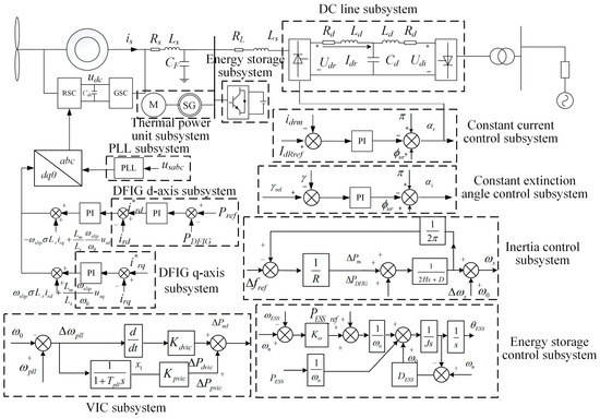
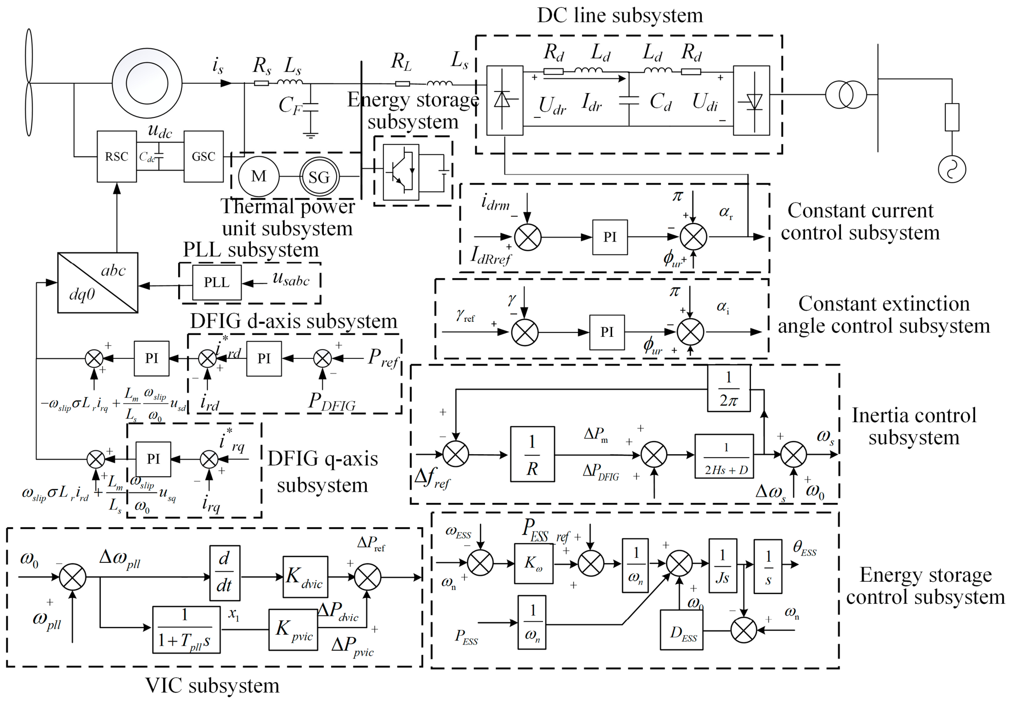
The multi-source integrated HVDC sending-end system investigated in this paper is illustrated in Figure 1. The doubly fed wind farm consists of multiple doubly fed induction generator (DFIG) units, each operating under a maximum power point tracking (MPPT) control strategy. Together with thermal power units and the energy storage system, the DFIG-based wind farm is connected to the sending-end AC bus and delivers power to the line-commutated converter high-voltage direct current (LCC-HVDC) transmission system. The LCC-HVDC system adopts a bipolar terminal structure, in which the rectifier-side converter station employs a constant-current control strategy, while the inverter-side converter station adopts a constant extinction angle control strategy.
Figure 1.
Topological Diagram of Multi-Infeed DC System.
Considering the transient and sub-transient processes of the synchronous generator, the sub-transient and transient electromotive forces (EMFs) of the rotor d-axis damping winding and excitation winding, as well as those of the q-axis damping windings, are taken into account. In addition, under N–m fault conditions, significant active power deficits may arise in the system. In such scenarios, the primary frequency regulation subsystem of thermal power units plays a crucial role in providing frequency support to the system. The corresponding model is formulated as follows:
- (1)
- Mathematical Model of the Thermal Power Unit Inertia Subsystem
- (2)
- Mathematical Model of the Thermal Power Unit d-Axis Subsystem
- (3)
- Mathematical Model of the Thermal Power Unit q-Axis Subsystem
- (4)
- Mathematical Model of the Virtual Inertia Control Section Subsystem
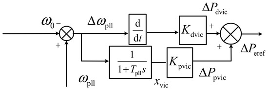
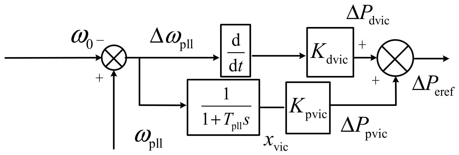
As shown in Figure 2, virtual inertia control combines the rate of change in grid frequency with a proportional link to dynamically adjust the active power reference of the converter. This enables wind turbines to emulate the rotational inertia response characteristics of synchronous generators, thereby providing inertia support to the power grid. From Figure 2, the standard form of the second-order equation for the virtual inertia subsystem is constructed as follows:
where and are the proportional coefficients of the differential link and the first-order lag link in the virtual inertia subsystem, respectively; is the variation in the phase-locked loop (PLL) speed; is the time constant of the droop control module; is the state variable of the current first-order lag chain; is the reference value of the state variable for the current first-order lag chain; and is the variation in the power command value of the doubly fed induction generator (DFIG).
Figure 2.
Topological Diagram of the Virtual Inertia Control Section.
- (5)
- Mathematical Model of the Phase-Locked Loop Subsystem
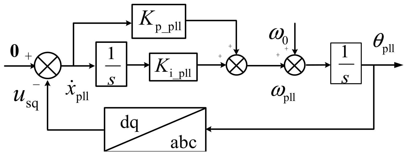
The phase-locked loop (PLL) can quickly track the phase angle and frequency at the point of common coupling (PCC) of the doubly fed induction generator (DFIG), thus realizing grid voltage-oriented control. As shown in Figure 3, the standard form of the second-order equation for the three-phase synchronous PLL control of the DFIG is constructed as follows:
where is the state variable of the integral link in the current proportional-integral (PI) controller; and are the proportional and integral coefficients of the PI controller in the phase-locked loop (PLL) subsystem, respectively.
Figure 3.
Topological Diagram of the Phase-Locked Loop Section.
- (6)
- Mathematical model of the doubly fed induction generator (DFIG) d-axis subsystem
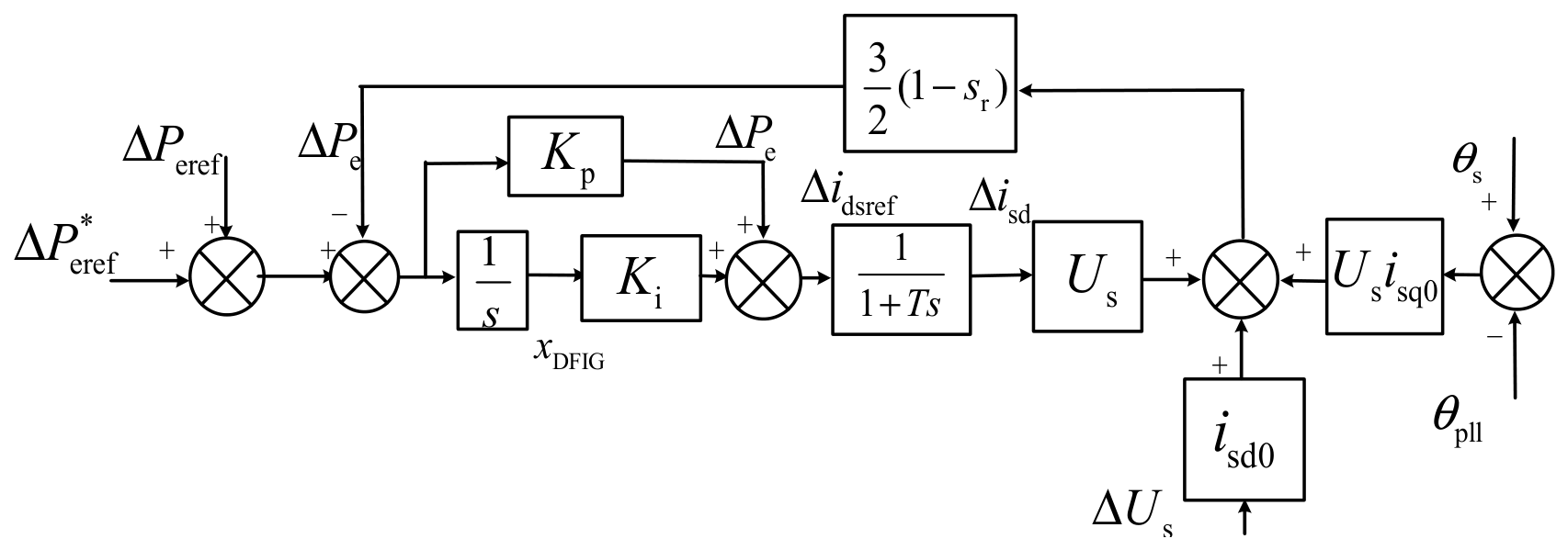
For the doubly fed induction generator adopting grid voltage-oriented control, the incremental equation of the electromagnetic power of the DFIG can be derived as:
Since the objective of this study is to evaluate the cumulative energy interaction among subsystems and its influence on transient stability, rather than the detailed electromagnetic transient responses of individual electrical variables, the current-control inner loop can be treated as a fast subsystem. Given that its response time is on the order of milliseconds, while the cumulative energy index is evaluated by integrating the energy variation rate over a several-second time horizon, the short-term dynamic discrepancies introduced by the approximation have a negligible effect on the calculated cumulative energy. Therefore, the current-control inner loop is represented by an equivalent first-order inertial element without compromising the accuracy of the transient stability assessment. In addition, a time-domain comparison between the detailed current-control loop model and the first-order inertial approximation has been provided in Appendix B to further validate the effectiveness and accuracy of the proposed simplification. Finally, the stator dq-axis currents can be obtained as:
where and are the integral and proportional coefficients of the outer power loop in the d-axis subsystem of the doubly fed induction generator (DFIG), respectively; is the d-axis time constant of the DFIG converter; is the variation in the d-axis stator current of the DFIG; and is the variation in the reference value of the d-axis stator current command for the DFIG.
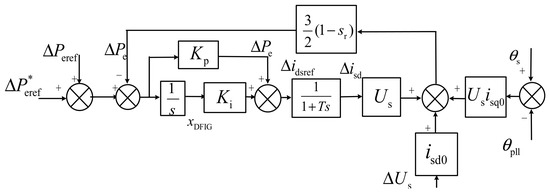
Thus, the block diagram of the incremental transfer function for the electromagnetic power of the DFIG-based wind turbine is obtained, as shown in Figure 4:
Figure 4.
Topological Diagram of the Increment of Electromagnetic Power in DFIG.
From Figure 4, the standard form of its second-order equation is derived as:
where is the state variable of the integral link in the current loop PI controller; is the variation in the d-axis stator current of the doubly fed induction generator (DFIG); is the d-axis stator current of the DFIG under normal operating conditions of the sending-end system.
The detailed mathematical models and their derivation processes for the DFIG q-axis subsystem, rectifier-side subsystem, DC line subsystem, inverter-side subsystem, energy storage active power control subsystem, and energy storage reactive power control subsystem are presented in Appendix A. Substituting the standard form of the second-order mathematical model of each subsystem into Equation (14), the energy function can be obtained, which is given by Equations (A1)–(A6), (A8), (A14), (A21), (A23), (A25) and (A27), respectively.
The energy model developed in this paper is applicable to operating scenarios in which the system topology and control modes remain unchanged after a disturbance. Following an N–m contingency, a significant power imbalance may occur in the sending-end system, and regulating units such as synchronous generators and energy storage systems participate in the dynamic regulation process to maintain system stability. Since the proposed energy model can characterize the energy exchange among subsystems and the dynamic evolution of system energy, it remains valid as long as the disturbance only causes deviations in the operating state without altering the system control structure.
When a disturbance is severe enough to trigger control mode switching or protection actions, the system dynamic equations and energy transfer mechanisms may change. Examples include an LCC-HVDC system entering the Voltage Dependent Current Order Limiter (VDCOL) mode or forced commutation angle control mode, wind turbines entering Low-Voltage Ride-Through (LVRT) mode, or changes in the system topology. Under such conditions, a new energy model must be established according to the updated control mode. Therefore, the energy model proposed in this paper is primarily applicable to transient stability analysis under the assumption that the control structure and control logic remain unchanged.
3. Parameter Optimization Method for Multi-Infeed DC Sending-End Systems
The energy model is developed based on incremental state variables around the operating equilibrium point. The system dynamics are described by the deviations of state variables from their equilibrium values, which enables the dominant post-fault dynamic behaviors and energy transfer mechanisms to be captured while reducing the complexity of the multi-source HVDC system analysis. The objective of this study is to reveal the energy evolution mechanisms and the relative impacts of different control loops on transient stability rather than to reproduce all nonlinear dynamic behaviors under extreme disturbances. Therefore, when the system operates within its normal control regime and the state deviations remain within an acceptable engineering range, the proposed model can accurately characterize the energy interaction characteristics of the system. However, under extreme operating conditions involving large state deviations or strongly nonlinear behaviors, the model accuracy may be affected and a new model should be established according to the updated operating conditions.
Based on the above modeling assumption, each state variable can be decomposed into a steady-state component and a fault-induced deviation component. Therefore, the instantaneous value of an arbitrary state variable can be expressed as:
where is the instantaneous value of an arbitrary state variable in the system; is the steady-state value of the state variable; and is the variation of the state variable.
Its fault component satisfies the following standard form of the function:
where , , and are the generalized capacitance, inductance, and resistance, respectively; , , and are constant terms; and are the fault components of the generalized voltage and current, respectively. The interactive links affecting voltage are uniformly denoted as , and those affecting current are uniformly denoted as . The purpose of introducing the generalized inductance and capacitance is to facilitate the definition of energy terms corresponding to control parameters. Different subsystems are connected through the interactive links and .
The first integral method [20,21] is employed to transform the state-space dynamic equations into an energy-based representation and to construct the system energy function. Perform cross-multiplication on Equation (11) yields:
Integrating Equation (12) yields:
Based on Equation (13), the energy model of the system can be constructed and expressed as:
where the first and second terms in represent the electric field energy stored in the generalized capacitance and the electromagnetic energy stored in the generalized inductance , respectively. denotes the dissipated energy on the generalized resistance . denotes the interaction energy between this system and other subsystems. In , the first term reflects the interaction energy through the interactive link , and the second term reflects the interaction energy through the interactive link . It can be seen from that each interactive link corresponds to an interaction energy term.
Differentiating the stored energy of the DC sending-end system with respect to time yields:
In Equation (15), an energy balance relationship is established among the stored energy, dissipated energy, and interaction energy. Based on this relationship, the evolution of the stored energy can be quantitatively interpreted through the dissipated energy and the interaction energy . It should be noted that the interaction energy represents the energy transfer among internal subsystems, while the dissipated energy represents the cumulative energy consumed by damping mechanisms. Therefore, Equation (15) describes the energy balance within the overall system rather than the conservation of stored energy itself. According to Lyapunov’s second method, the stability of a disturbed system can be characterized by the evolution of its stored energy. If the stored energy gradually decreases with time, the oscillation amplitude decays and the system converges to the equilibrium point. Conversely, if the stored energy continuously increases, the system tends toward instability. Furthermore, according to Equation (14), the derivative of the stored energy is jointly determined by the derivatives of dissipated energy and interaction energy. The derivative of dissipated energy is always negative, representing energy consumption caused by damping and control actions, which promotes the decay of stored energy and enhances system stability. In contrast, the sign of the interaction energy derivative depends on the direction of energy transfer among subsystems. A positive interaction energy derivative contributes to energy accumulation and may deteriorate system stability, whereas a negative interaction energy derivative suppresses energy accumulation and supports system stability. Therefore, transient stability is assessed by analyzing the influence of dissipated energy and interaction energy on the evolution of stored energy.
To investigate the influence of key control links on the stability of the multi-source-integrated DC sending-end system, the energy functions of all subsystems are first summed to obtain the energy function of the multi-source-integrated DC system:
where is the energy function of the thermal power plant module; is the energy function of the doubly-fed induction generator (DFIG) module; is the energy function of the DC module; and is the energy function of the energy storage module.
The structure of the energy function for each module is given by Equation (17):
On this basis, the interaction strength is defined as shown in Equation (18):
where is the rate of change in the interaction energy between subsystems, and k is the key control parameter.
The interaction strength is derived based on the analytical interaction energy model established in this paper. Specifically, the interaction energy rate is first obtained by differentiating the interaction energy function with respect to time. Subsequently, the measured electrical quantities of each subsystem are substituted into the corresponding interaction energy rate expressions. Based on these expressions, the interaction strength is obtained by taking the partial derivative of the interaction energy rate with respect to the investigated control parameter. Therefore, the interaction strength quantitatively characterizes the sensitivity of the interaction energy transfer process to variations in a specific control parameter.
It should be noted that the interaction strength is calculated directly from the analytical expression without additional normalization. The purpose of the proposed index is to evaluate the influence of a given control parameter on the interaction energy transfer process within its predefined feasible operating range. Since the analysis is performed within the feasible variation range of each controller parameter, the conclusions are drawn based on the variation trend of the interaction strength rather than its absolute numerical value. Therefore, additional normalization is not required. The interaction strength represents the sensitivity of the interaction energy rate to variations in the control parameters of the key control loops in each subsystem. Furthermore, the sign of the interaction strength indicates the direction of the influence of a control parameter on the interaction energy transfer process. By examining its sign, it can be determined whether an increase in the corresponding control parameter promotes or suppresses interaction energy accumulation, thereby allowing its impact on system transient stability to be assessed:
(1) When the interaction strength , the rate of change in interaction energy increases monotonically with the control parameter . At this time, if the control parameter is increased:
- -
- When , the positive energy accumulated by the control link will increase, showing a divergent trend, which is unfavorable to system stability.
- -
- When , the negative energy accumulated by the control link will decrease, so the negative energy cannot further converge to a larger value, which is also unfavorable to system stability.
(2) When the interaction strength , the rate of change in interaction energy decreases monotonically with the control parameter . At this time, if the control parameter is increased:
- -
- When , the positive energy accumulated by the control link will decrease, showing a trend of converging to a negative value, which is beneficial to system stability.
- -
- When , the negative energy accumulated by the control link will increase and converge to a larger value, which is also beneficial to system stability.
Therefore, when the interaction strength , increasing the control parameter is beneficial to system stability; when the interaction strength , increasing the control parameter is unfavorable to system stability.
- (1)
- Impact of DFIG d-axis control parameters on stability
Taking the partial derivatives of Equation (A6) with respect to the proportional coefficient and the integral coefficient of the PI controller in the d-axis subsystem of the doubly fed induction generator (DFIG), we have:
From Equation (19), since the phase-locked loop (PLL) tracks the system phase angle on the transient time scale of N-m faults, the difference between its value and the system phase angle is small. Therefore, the variation in the locked phase angle of the DFIG PLL, , is close to the variation of the system phase angle, , i.e., . It follows that . Therefore, increasing the proportional coefficient of the DFIG d-axis subsystem reduces the energy consumed by its own self-interaction energy links and the interaction energy links with other subsystems, which is unfavorable to system stability. For the interaction strength , changing the integral coefficient of the PI controller in the DFIG d-axis subsystem has almost no effect on its own self-interaction energy links and the interaction energy links with other subsystems.
- (2)
- Impact of energy storage control parameters on stability
Taking the partial derivatives of Equations (A25) and (A26) with respect to the frequency regulation coefficient and the reactive power-voltage droop coefficient of the energy storage subsystem, we have:
From Equation (20), since , increasing the frequency regulation coefficient of the energy storage subsystem will increase the energy consumed by its own self-interaction energy links and the interaction energy links with other subsystems, which is beneficial to system stability. For the interaction strength , increasing the reactive power-voltage droop coefficient of the energy storage subsystem will also increase the energy consumed by its own self-interaction energy links and the interaction energy links with other subsystems, which is beneficial to system stability.
- (3)
- Impact of LCC rectifier-side control parameters on stability
Taking the partial derivatives of Equation (A14) with respect to the proportional coefficient and the integral coefficient of the PI controller on the LCC rectifier side, we have:
From Equation (21), since , increasing the proportional coefficient of the LCC rectifier-side subsystem will increase the energy consumed by its own self-interaction energy links and the interaction energy links with other subsystems, which is beneficial to system stability. For the interaction strength , changing the integral coefficient of the PI controller in the LCC rectifier-side subsystem has almost no effect on its interaction energy links with other subsystems.
System parameters are optimized to minimize the accumulated total energy after N-m fault recovery. The specific optimization objects include parameters of the energy storage side, the doubly fed induction generator (DFIG) side, and the DC side. Due to the inherent flexibility and fast response capability of the energy storage system, its frequency regulation parameters directly affect the active power support effect, while the droop parameters determine the grid-connected dynamic characteristics.
The proportional and integral parameters of the active power outer loop on the DFIG side affect its active power response characteristics. The constant current proportional and integral parameters on the DC side control the output power by regulating the magnitude of the transmitted current. Optimizing these parameters can effectively improve the overall system performance.
- (1)
- Impact of the DFIG active power proportional parameter and integral parameter on stability
Taking the partial derivatives of Equation (A6) with respect to the active power proportional parameter and integral parameter , we have:
From Equations (22) and (23), the rate of change in the accumulated energy of the DC sending-end system with respect to the DFIG active power proportional parameter and integral parameter is a nonlinear equation with variables. Its monotonicity cannot be directly determined, so an optimization algorithm is required to find its minimum point.
- (2)
- Impact of the energy storage subsystem frequency regulation coefficient and reactive power-voltage droop coefficient on stability
Taking the partial derivatives of Equations (A25) and (A26) with respect to the virtual synchronous machine frequency regulation coefficient and the reactive power-voltage droop coefficient , we have the following:
From Equation (24), since , increasing the virtual synchronous machine frequency regulation coefficient reduces the accumulated energy of the system, which is beneficial to system stability. From Equation (25), since , increasing the reactive power-voltage droop coefficient also reduces the accumulated energy of the system, which is beneficial to system stability.
- (3)
- Impact of the DC-side constant current control proportional parameter and integral parameter on stability
Taking the partial derivatives of Equation (A14) with respect to the constant current control proportional parameter and integral parameter , we have:
From Equations (26) and (27), since , increasing the DC-side constant current control proportional parameter increases the accumulated energy of the system, which is unfavorable to system stability; since , increasing the DC-side constant current control integral parameter reduces the accumulated energy of the system, which is beneficial to system stability.
- (1)
- Objective Function
After quantitatively analyzing the impact of energy storage integration on the stability of the DC sending-end system, this study takes the DC sending-end system under N-m faults as the main research object, and proposes a strategy to support unbalanced power through the control parameters of the DC sending-end system. Specifically, by adjusting the parameters of the doubly fed induction generator (DFIG), energy storage, and DC system, the energy accumulation in each link of the DC sending-end system after an N-m fault can be minimized. This problem can be described by constructing an optimization model with additional constraints.
It should be noted that although the DFIG, energy storage system (ESS), and DC subsystem operate on different time scales, the objective function adopted in this paper is constructed based on the cumulative energy of the entire system. Since energy is a physical quantity capable of providing a unified representation of dynamic processes across different time scales, the dynamic responses of all subsystems are ultimately reflected in the cumulative energy index. Specifically, fast dynamics mainly affect the instantaneous energy variation, whereas slow dynamics influence the long-term energy accumulation, both of which are incorporated through the energy integration process. Therefore, the proposed objective function can integrate multi-timescale dynamic characteristics into a unified optimization framework, enabling the coordinated optimization of DFIG, ESS, and DC-side control parameters from the perspective of overall system transient stability.
- (2)
- Constraints
In addition to ensuring power balance, several additional constraints are introduced to comprehensively consider system dynamic response, energy storage operation limits, and inertia that can guarantee system frequency support:
(1) Active Power Balance Constraint
After an N-m fault, an active power imbalance occurs at the sending-end AC tie line. The coordinated regulation of wind power, thermal power, HVDC, and energy storage can maintain power balance, which must satisfy:
(2) Energy Storage Power Output Constraint
The charging and discharging power of the energy storage system is limited by its rated power:
(3) Unit Output Constraint
Both thermal power units and doubly fed induction generators (DFIGs) must generate power within their respective regulation capabilities:
(4) Energy Storage Parameter Adjustment Constraints
The frequency regulation coefficient and the reactive power-voltage droop coefficient of the energy storage virtual synchronous machine must satisfy the system frequency and voltage stability requirements:
(5) DFIG Parameter Adjustment Constraints
The active power proportional parameter and integral parameter of the doubly fed induction generator (DFIG) must satisfy the following limits:
(6) DC-Side Constant Current Control Parameter Adjustment Constraints
The proportional parameter and integral parameter of the DC-side constant current control must satisfy the following limits:
- (3)
- Optimization Scheme
The Butterfly Optimization Algorithm (BOA) is a swarm intelligence optimization algorithm proposed by Arora in 2019 [21]. It has the advantages of simple parameter adjustment and strong global search capability. To further evaluate the optimization performance and effectiveness of the proposed IBOA-based parameter tuning method, comparative simulations were conducted using four representative optimization algorithms, namely GA, PSO, BOA, and IBOA. For a fair comparison, all algorithms were implemented under identical optimization conditions, including the same population size, maximum iteration number, optimization variables, search domains, and objective function. The optimization results are summarized in Table 1.
Table 1.
Quantitative Comparison of Different Optimization Algorithms.
As shown in Table 1, all four algorithms can successfully obtain feasible solutions for the controller parameter optimization problem. However, the proposed IBOA achieves the lowest objective function value and the fastest convergence speed among all compared methods. Compared with GA, PSO, and BOA, the convergence iteration number of IBOA is significantly reduced while obtaining a better optimization result.
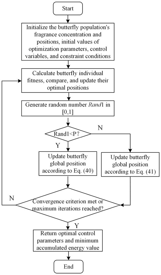
In this algorithm, each butterfly interacts with others by releasing scents of certain concentrations, and dynamically chooses between global and local search using a switching probability : if , it performs global search; otherwise, it performs local search. The basic update process is as follows: the scent intensity of each butterfly is determined by stimulus intensity. Global search is achieved by guiding individuals toward the current optimal position, while local search is completed through information exchange between random individuals. The Improved Butterfly Optimization Algorithm (IBOA) introduces an adaptive weight coefficient and embeds it into the update formulas for local and global search. This weight coefficient changes dynamically during the iteration process: in the early stage of optimization, it weakens the guiding effect of the optimal individual to enhance global exploration capability; in the later stage, it gradually strengthens the influence of the optimal individual, thereby accelerating the convergence of individuals near the optimal solution.
The formulas for scent generation, global search, and local search by butterflies are as follows:
where is the stimulus intensity; is the modality power exponent; is the sensory factor of the butterfly; is the perceived intensity of the scent; is the spatial position of the -th butterfly after iterations; and are the random spatial positions of the -th and -th butterflies after iterations; is any number in ; represents the scent concentration of the -th butterfly; is the position of the best-fit butterfly in the t-th iteration. Specifically, the population size was set to 30, the maximum number of iterations was set to 500, the sensory modality parameter was initialized as 0.01, the power exponent was set to 0.1, and the switching probability was set to 0.8. The optimization process was terminated when the maximum iteration number was reached. The specific optimization steps are as follows:
Step 1: Initialize system parameters and the butterfly population. Obtain initial values of control parameters based on the system model, and preliminarily determine the parameter optimization range according to the objective function and constraints. Set the butterfly population size and the maximum number of iterations , then initialize the butterfly population.
Step 2: Calculate the fitness value of each butterfly individual based on the objective function, and assume the current best-fit butterfly individual is . By comparing the fitness value of the current butterfly with the optimal butterfly individual , if is lower than , discard the butterfly individual and keep the current butterfly position; otherwise, discard and output the current best butterfly individual position. Check the generation condition: if met, output the optimal control parameter values; otherwise, proceed to the next operation to determine whether to perform local or global flight.
Step 3: Generate a random number from . If is less than the switching probability , perform global flight and update the global position according to Equation (40); otherwise, perform local flight and update the local position according to Equation (41). If the maximum number of iterations is reached, output the optimal control parameter solution and the minimum accumulated energy value; otherwise, return to Step 2.
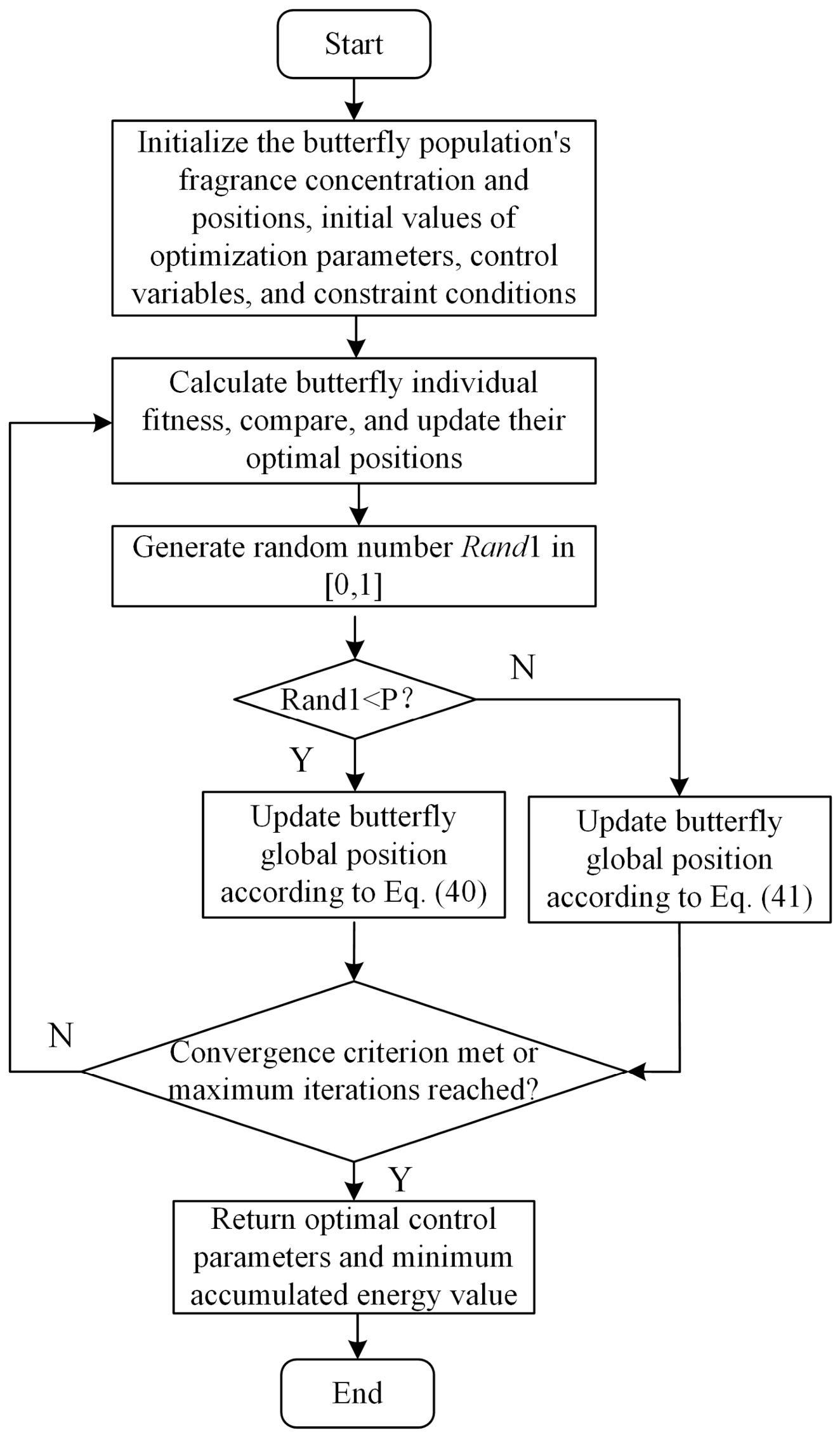
The parameter optimization flowchart is shown in Figure 5.
Figure 5.
Flowchart of Parameter Optimization Strategy.
4. Simulation Verification
4.1. Verification and Analysis of Transient Stability of the Multi-Source Integrated DC Sending-End System
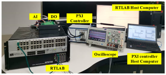
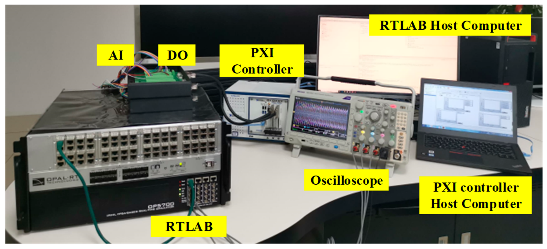
A hardware-in-the-loop simulation model is established on the RT-LAB platform to verify the stability of key control links in the multi-source integrated DC sending-end system. Based on the RT-LAB hardware-in-the-loop experimental platform, the modeling and parameter tuning are firstly completed in MATLAB/Simulink 2024. Then the PXI upper computer is connected to RT-LAB, and an oscilloscope is also linked to the platform. The established simulation model is downloaded to the hardware-in-the-loop experimental platform via a computer, and the measurement data are finally acquired from the oscilloscope. The RT-LAB simulation platform is presented in Figure 6, which is adopted to validate the conclusions drawn in this paper. Compared with conventional offline simulations, the RT-LAB-based HIL platform enables real-time interaction between controllers and the power system model while considering practical factors such as signal sampling, communication delays, and controller execution processes. As a result, the validation results exhibit higher engineering fidelity and realism.
Figure 6.
Hardware-in-loop Test Platform.
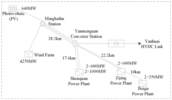
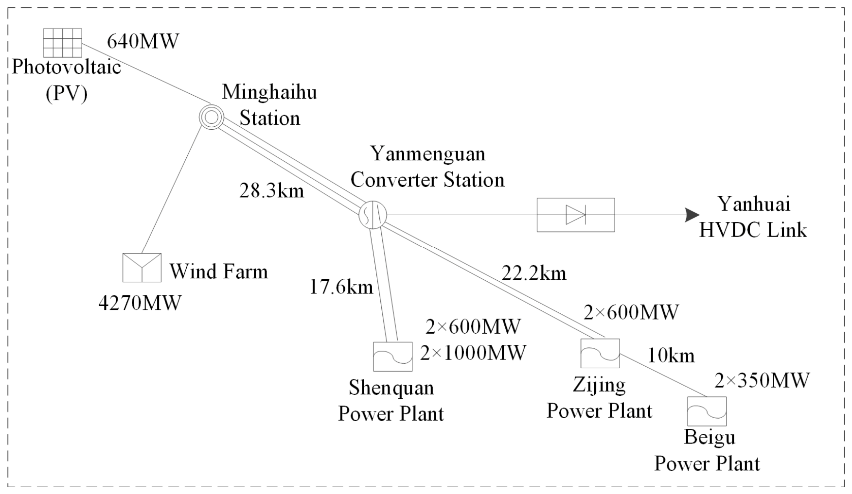
The Hardware-in-the-Loop (HIL) simulation system is established on the RT-LAB real-time digital simulation platform using the practical configuration of the commissioned Yanhuai ±800 kV UHVDC transmission project as the prototype, and its topology is shown in Figure 7. The system parameters, control structures, and operating conditions are configured according to the actual engineering specifications to ensure that the developed experimental model can accurately reflect the dynamic characteristics of a practical HVDC sending-end system. By incorporating a real-world engineering background, the constructed HIL platform not only enables real-time interaction between controllers and the power system model but also significantly enhances the engineering realism and credibility of the validation results, thereby providing strong support for the practical applicability of the proposed method.
Figure 7.
Topology Diagram of Yanhuai ±800 kV UHVDC Transmission System.
The Yanhuai UHVDC project starts at Yanmenguan in Shuozhou, Shanxi Province and terminates at Huai’an, Jiangsu Province. As a key corridor for China’s West-to-East and North-to-South power transmission initiatives, it bundles thermal and wind power resources in northwestern Shanxi and delivers them to East China. The DC terminal of this system has a rated power of 8000 MW and a voltage level of ±800 kV. When an N-2 fault occurs on the Huguan transmission line, the Yanhuai UHVDC system is electrically disconnected from the main AC grid, and local power plants together with the DC sending-end system operate without main grid support.
In the simulation, the AC grid is disconnected at 5.0 s to emulate the N-2 fault of the DC sending-end system. Disconnection from the AC grid will cause a large active power deficit and further lead to system instability.
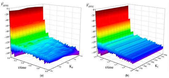
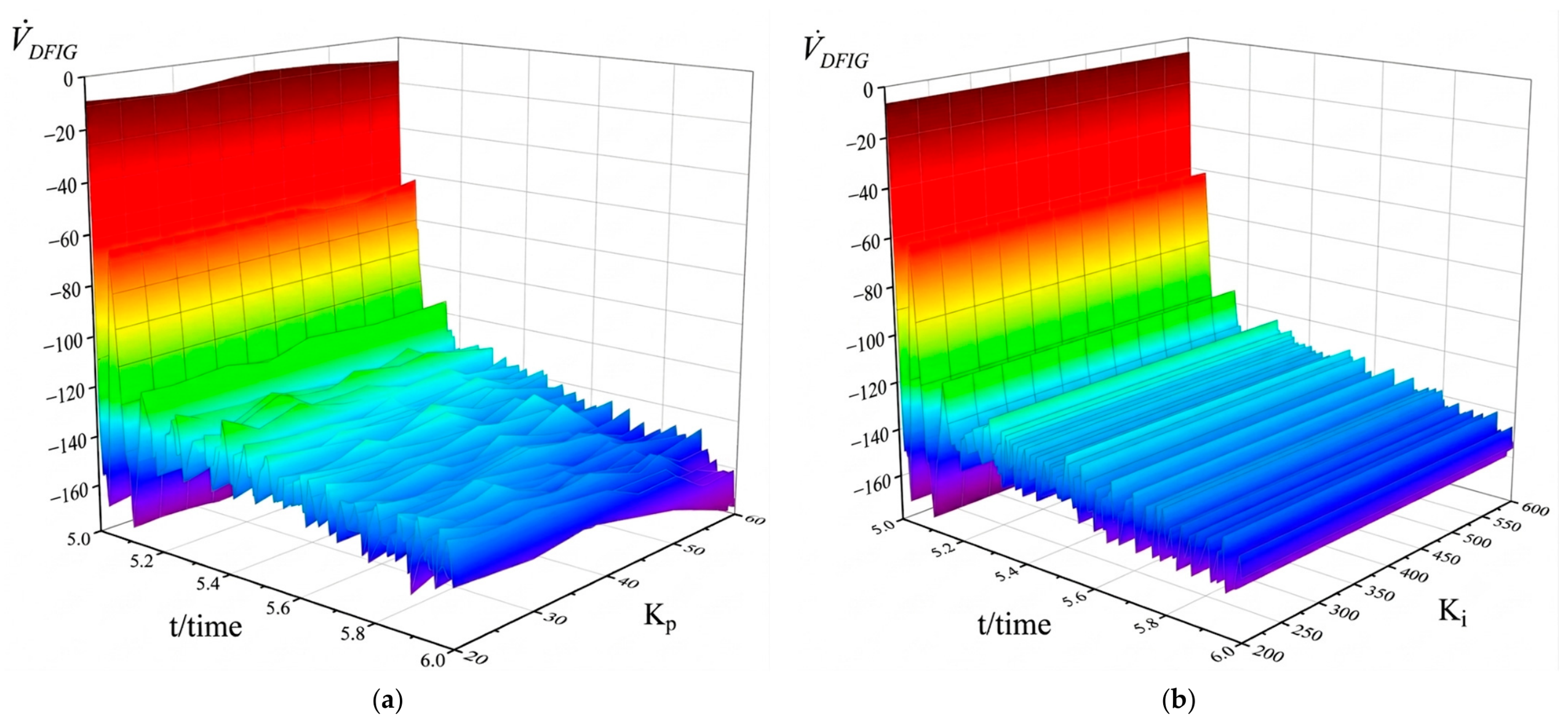
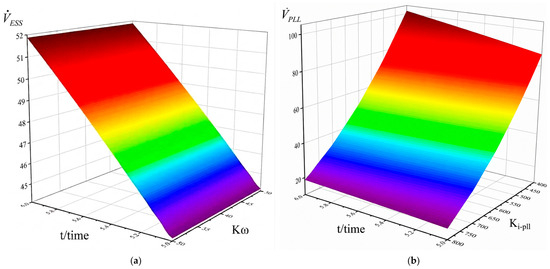
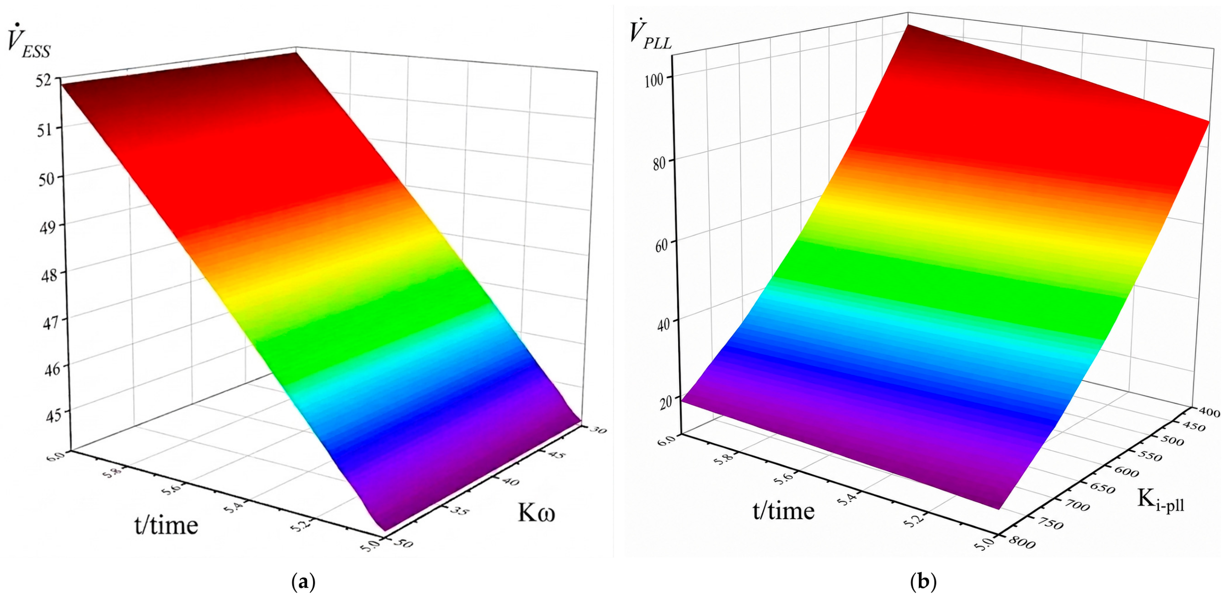
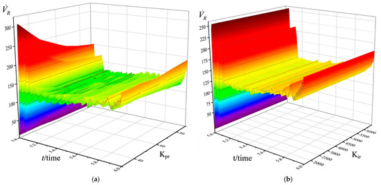
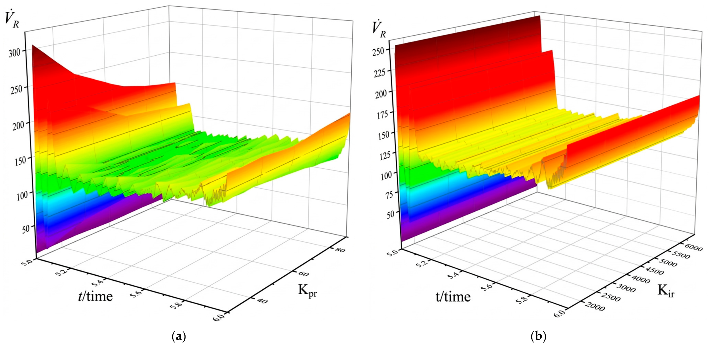
Simulation verifications are carried out to validate the stability analysis of key control links in the multi-source integrated DC sending-end system. Figure 8, Figure 9 and Figure 10 present a three-dimensional parameter-sensitivity analysis. The horizontal axis represents the controller parameter, the vertical axis represents time, and the depth axis denotes the interaction-energy rate. The purpose of this figure is to reveal the transient energy evolution characteristics under different controller parameter settings and to quantify the influence of parameter variations on system stability from an energy perspective. The color scale follows a red-to-blue spectrum, where warmer colors (red and yellow) indicate higher energy levels and cooler colors (blue and purple) indicate lower energy levels.
Figure 8.
The Influence of DFIG d-axis Control Parameters on Stability. (a) The variation in parameter and the resulting interaction energy; (b) The variation in parameter and the resulting interaction energy.
Figure 9.
The Influence of Energy Storage Control Parameters on Stability. (a) The variation in parameter and the resulting interaction energy; (b) The variation in parameter and the resulting interaction energy.
Figure 10.
The Influence of LCC Constant Current Control Parameters on Stability. (a) The variation in parameter and the resulting interaction energy; (b) The variation in parameter and the resulting interaction energy.
- (1)
- Influence of DFIG d-axis control parameters on stability
As shown in Figure 8, the rate of energy change in the DFIG d-axis control subsystem is always negative, and its magnitude increases with time. Increasing the proportional coefficient of the DFIG d-axis subsystem will increase the rate of energy change, which means that the self-interaction energy links and the interaction energy links with other subsystems consume less energy, which is unfavorable to system stability. Changing the integral coefficient of the PI controller in the DFIG d-axis subsystem has almost no effect on the rate of energy change, and thus has negligible impact on the self-interaction energy links and the interaction energy links with other subsystems.
- (2)
- Influence of energy storage control parameters on stability
As shown in Figure 9, the rate of energy change in the energy storage subsystem is always positive, and its magnitude increases with time. Equation (20) indicates that the interaction strength associated with is proportional to the square of the system frequency deviation. Since the frequency deviation remains relatively small during the investigated transient process, the resulting interaction strength is inherently limited in magnitude. Moreover, the coefficient further reduces the numerical value of the interaction strength, leading to a relatively weak influence of on the overall energy accumulation process. Consequently, although increasing is beneficial to system stability, its contribution is relatively limited compared with the dominant control parameters identified in this paper. This is reflected in Figure 9a by the relatively flat variation trend of the interaction energy. Increasing the reactive power-voltage droop coefficient will reduce the rate of energy change, causing the interaction energy links with other subsystems to consume more energy, which is beneficial to system stability.
- (3)
- Influence of LCC rectifier-side control parameters on stability
As shown in Figure 10, the rate of energy change in the LCC constant current control subsystem is always positive, and its magnitude increases with time. Increasing the proportional coefficient of the LCC rectifier-side subsystem will reduce the rate of energy change, causing its own self-interaction energy links and the interaction energy links with other subsystems to consume more energy, which is beneficial to system stability. Changing the integral coefficient of the PI controller in the LCC rectifier-side subsystem has almost no effect on the rate of energy change, and thus has negligible impact on the interaction energy links with other subsystems.
4.2. Verification of Parameter Optimization of the Multi-Source Integrated DC Sending-End System
The active power proportional parameter and integral parameter of the DFIG, the proportional parameter and integral parameter of the DC-side constant current control, and the frequency regulation coefficient and reactive power-voltage droop coefficient of the energy storage system shall satisfy the following constraints:
After an N-m fault on the AC tie line of the DC sending-end system, to meet the transient stability constraints:
- -
- The energy storage frequency regulation coefficient is set in the range of , and the reactive power-voltage droop coefficient is set in the range of ;
- -
- Considering the operating power limit of the DFIG, the proportional parameter of the active power outer loop is set in the range of , and the integral parameter is set in the range of ;
- -
- To prevent DC blocking, the proportional parameter of the DC-side constant current control is set in the range of , and the integral parameter is set in the range of .
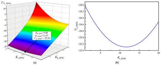
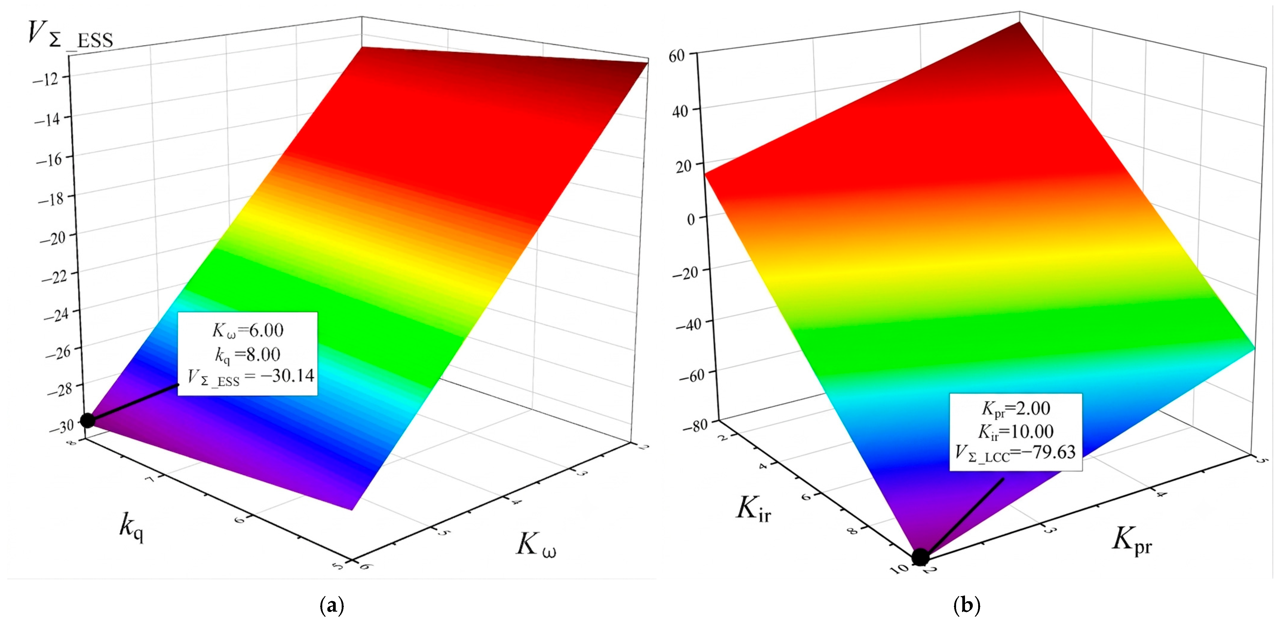
The relationship between the DFIG active power proportional parameter and integral parameter and the objective function value is shown in Figure 11. The color scale follows a red-to-blue spectrum, where warmer colors (red and yellow) indicate higher energy levels and cooler colors (blue and purple) indicate lower energy levels. It can be seen from the figure that, with the additional coordinated control, the accumulated energy of the DFIG forms an upward-opening parabola with respect to the parameter , indicating the existence of a minimum point, i.e., a local optimal solution. All local optimal solutions obtained through calculation are presented in Table 2.
Figure 11.
Cumulative Energy of Different Control Parameters on the DFIG Side. (a) Accumulated energy at wind turbine side under varied and ; (b) Profile of accumulated energy at wind turbine side with varied .
Table 2.
Local Optimal Solution.
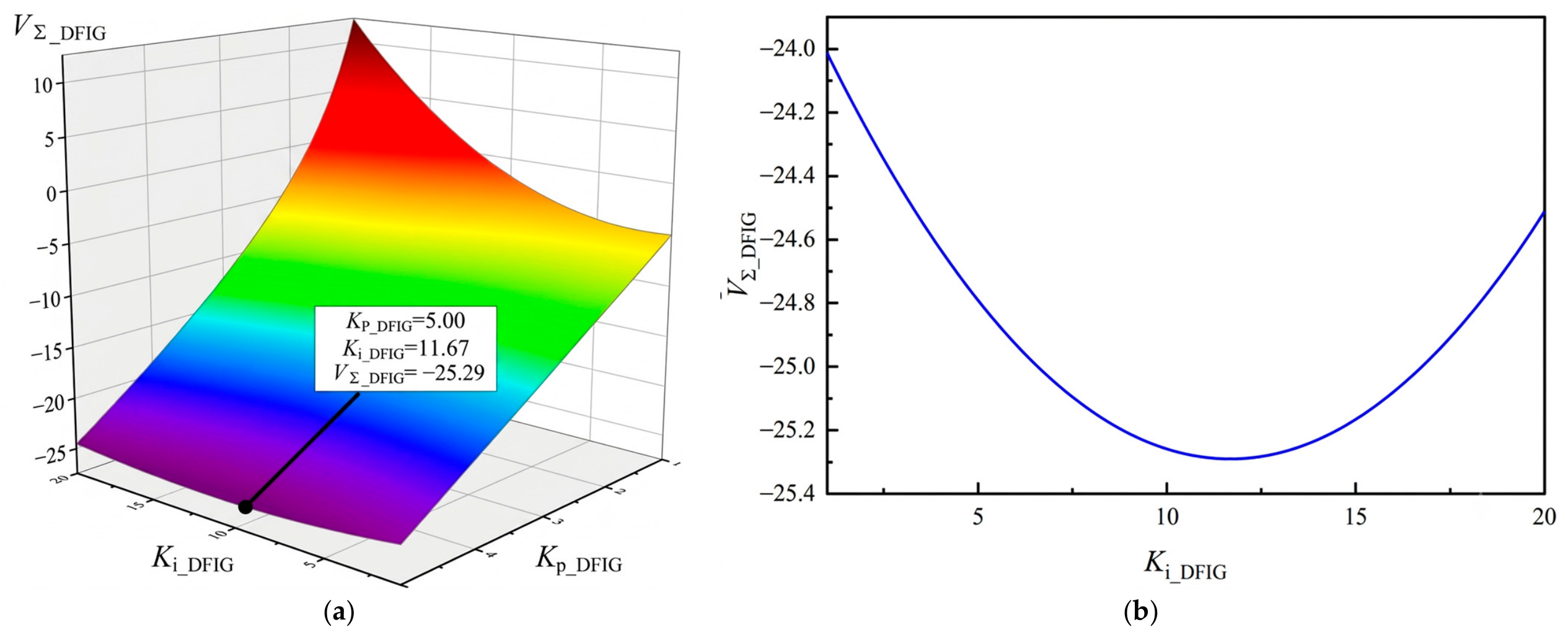
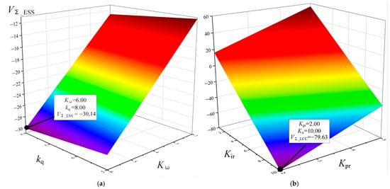
The relationships between the control parameters , , , and the objective function value are shown in Figure 12. The color scale follows a red-to-blue spectrum, where warmer colors (red and yellow) indicate higher energy levels and cooler colors (blue and purple) indicate lower energy levels. It can be seen that, within a certain parameter adjustment range, the accumulated energy is a monotonic function with respect to both the energy storage control parameters and the DC control parameters. Increasing the frequency regulation coefficient of the energy storage virtual synchronous machine reduces its accumulated energy, which is beneficial to system stability; increasing the reactive power-voltage droop coefficient also reduces its accumulated energy, which is beneficial to system stability. Increasing the proportional parameter of the DC-side constant current control increases its accumulated energy, which is unfavorable to system stability; increasing the integral parameter of the DC-side constant current control reduces its accumulated energy, which is beneficial to system stability. Therefore, under the system constraints, , , , and are the global optimal solutions that minimize the accumulated energy of the DC sending-end system.
Figure 12.
Cumulative Energy of Different Control Parameters on the Energy Storage and DC Side. (a) Accumulated energy of energy storage system under different control parameters; (b) Accumulated energy of DC system under different control parameters.
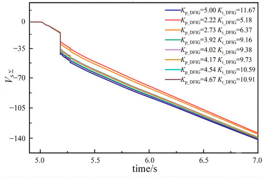
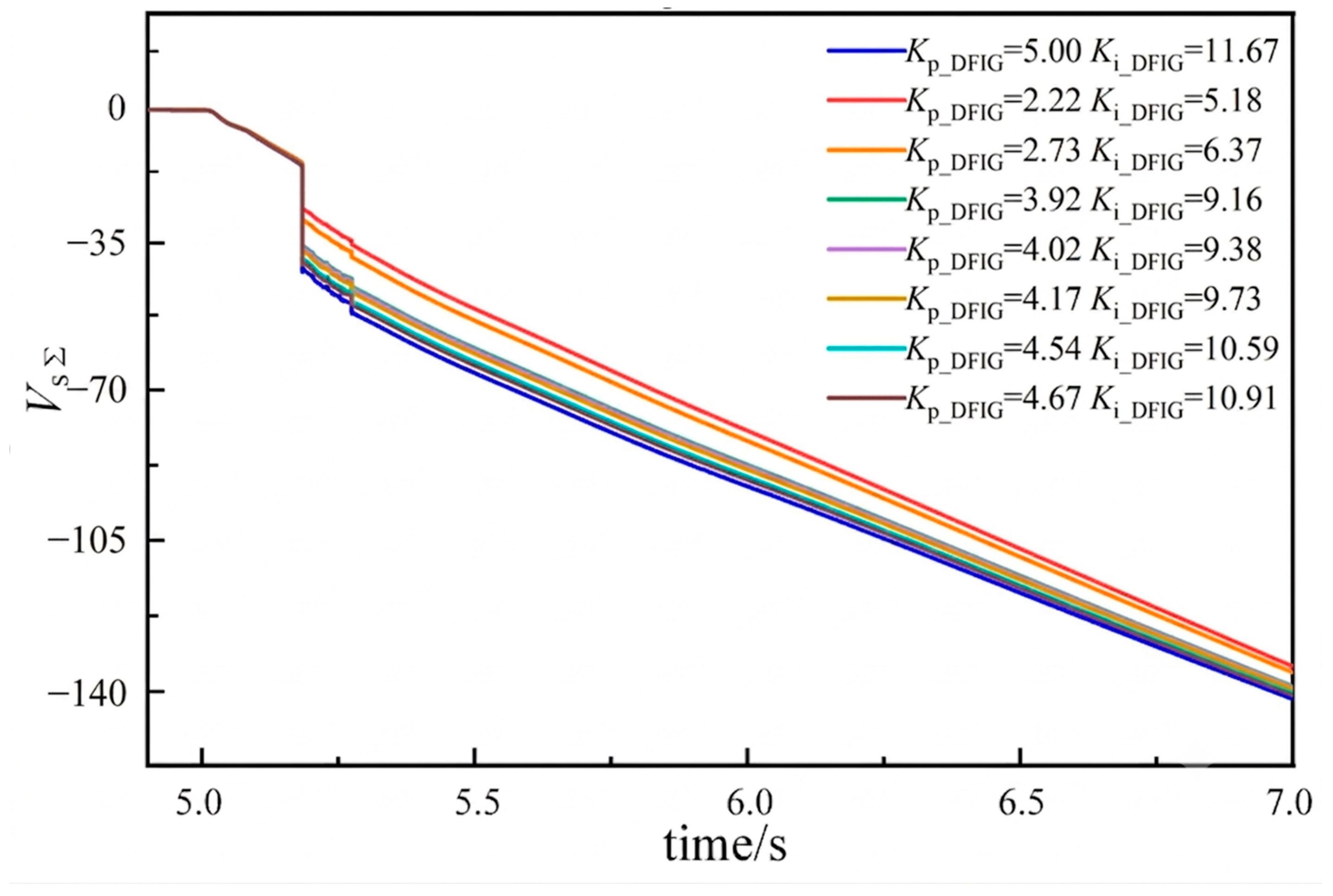
As shown in Figure 13, the local optimal solutions listed in Table 2 are substituted into the objective function to obtain the cumulative energy of the DC sending-end system at different time instants. The optimization process yields a set of candidate local optima, each corresponding to a different control-parameter combination. To identify the global optimum, the cumulative-energy characteristics associated with these candidate solutions are further compared and analyzed. Therefore, Figure 13 visualizes the screening process from local optimal solutions to the global optimal solution from the perspective of cumulative energy.
Figure 13.
Cumulative Energy of the DC Sending-end System with Different Control Parameters at Different Times.
The results show that the cumulative-energy trajectories corresponding to different local optimal solutions exhibit similar evolutionary trends, while their energy levels differ. By comparing the cumulative-energy responses of all candidate solutions, it can be observed that the parameter combination and consistently produces the lowest cumulative energy. This indicates that the corresponding solution achieves the best suppression effect on transient energy accumulation and can therefore be identified as the global optimal solution.
As listed in Table 3, the accumulated energy values of the DC sending-end system at 2 s after applying the additional coordinated control under the N-m fault are presented. It can be found that within the set of minimum solutions, the accumulated energy of the DC sending-end system reaches the minimum value of −135.0622 at and . This further verifies that and are the global optimal solutions for minimizing the accumulated energy of the DC sending-end system.
Table 3.
Cumulative Energy of the DC Sending-end System under Different Control Parameters.
In summary, the control parameters , , , and constitute the global optimal solution set that minimizes the accumulated energy of the DC sending-end system.
To evaluate the influence of parameter uncertainties on the optimization results, a ±20% perturbation was applied to the key system parameters, and the optimization procedure was repeated. The results are presented in Table 4.
Table 4.
Robustness Verification of Optimization Results Under Parameter Perturbation.
It can be observed that the optimal controller parameters obtained under parameter perturbations remain close to those of the nominal case, while only slight variations are observed in the minimum accumulated energy. Although parameter perturbations introduce certain deviations in the energy level, the optimal parameter combination and the overall optimization conclusions remain unchanged. This demonstrates that the proposed parameter optimization method possesses satisfactory robustness against reasonable parameter uncertainties.
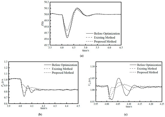
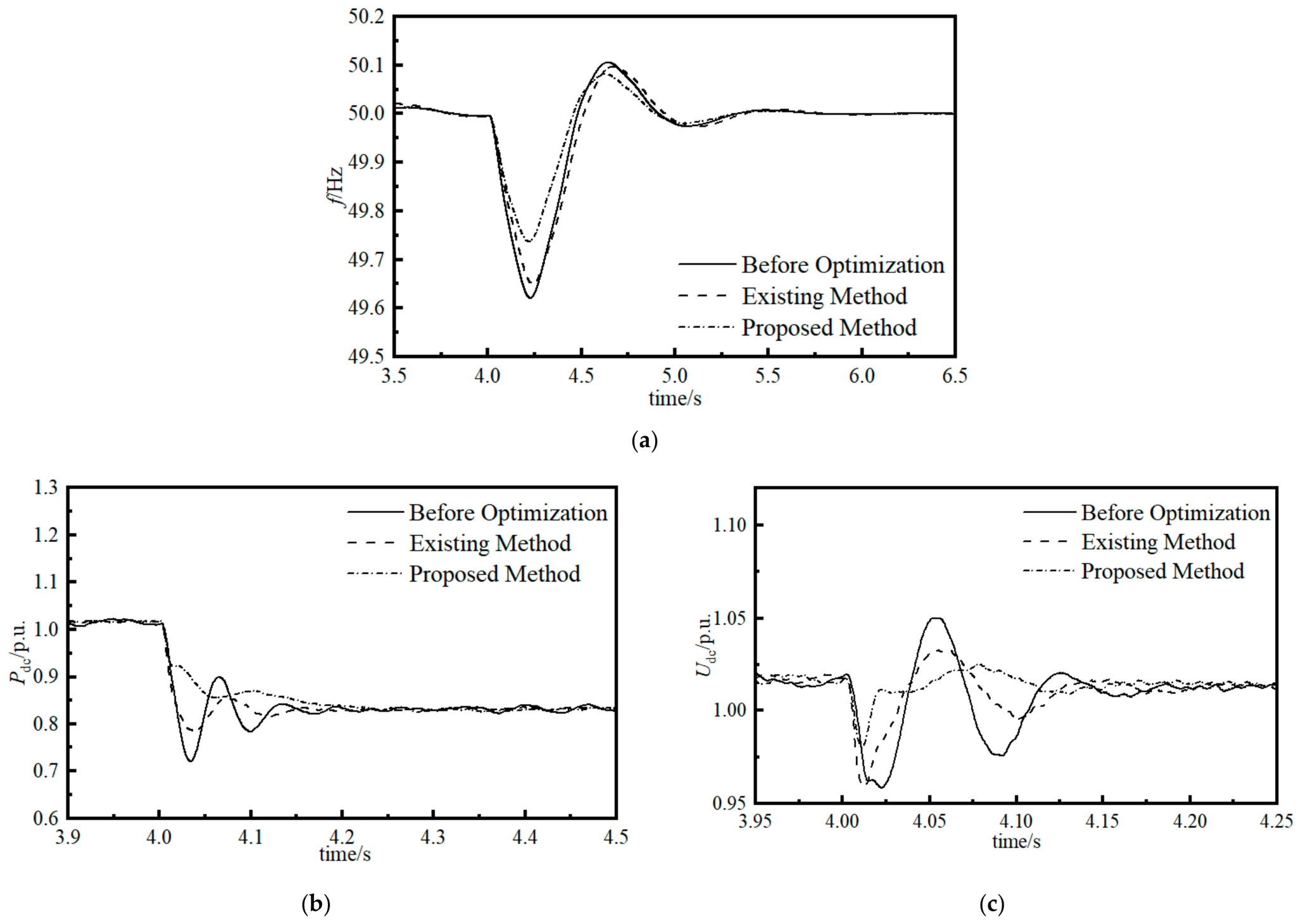
A comparative study is conducted between the method proposed in this paper and the control parameter optimization approach presented in Reference [22]. The simulation scenario is set as follows: an N-2 fault occurs on the AC tie line of the multi-source integrated DC system at t = 4 s. The system is disconnected from the main grid and operates in islanded mode, with approximately 60% of the total power capacity lost. The main electrical quantities of the system obtained by the existing parameter optimization method and the proposed method are illustrated in Figure 14.
Figure 14.
Main electrical quantities of the sending-end system during an N-2 fault on the AC interconnection line. (a) System frequency at sending end; (b) Transmitted power of DC side; (c) DC side voltage.
A large active power deficit occurs at the sending end, which leads to a drop in system frequency. Consequently, the frequency limit control (FLC) on the rectifier side is activated to reduce active power transmission. Meanwhile, thermal power units, wind turbines and the energy storage system rapidly output active power to participate in system regulation, and the system eventually maintains stable operation.
To provide a more quantitative evaluation of the optimization effectiveness, the key transient performance indicators before and after optimization are summarized in Table 5, including the maximum frequency deviation, active power deviation, DC voltage deviation, settling time, and stored energy.
Table 5.
Quantitative Comparison of Dynamic Performance Before and After Optimization.
It can be observed that the proposed method achieves smaller dynamic deviations, faster response recovery, and lower accumulated energy than both the unoptimized case and the existing optimization method, demonstrating its effectiveness in improving the transient stability performance of the multi-infeed DC sending-end system.
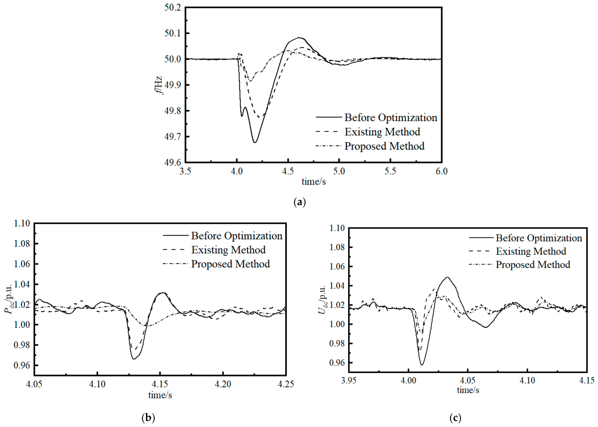
To verify the robustness and adaptability of the proposed method, an additional fault scenario is designed: an N-1 fault occurs on the AC tie line of the multi-source integrated DC system at t = 4 s. The system is disconnected from the main grid and operates in islanded mode, with approximately 40% of the total power capacity being lost. In this case, the wind power penetration level is increased to 50%, while all other operating conditions remain unchanged. The main electrical quantities of the system obtained by the existing parameter optimization method and the proposed method are illustrated in Figure 15.
Figure 15.
Main electrical quantities of the sending-end system during an N-1 fault on the AC interconnection line. (a) System frequency at sending end; (b) Transmitted power of DC side; (c) DC side voltage.
To provide a more quantitative evaluation of the optimization effectiveness, the key transient performance indicators before and after optimization are summarized in Table 6, including the maximum frequency deviation, active power deviation, DC voltage deviation, settling time, and stored energy.
Table 6.
Quantitative Comparison of Dynamic Performance Before and After Optimization.
It can be observed that, compared with the N–2 contingency, the N–1 fault corresponds to a less severe disturbance level. In this scenario, the governor and excitation systems of synchronous generators effectively mitigate the power imbalance caused by the fault, thereby maintaining stable system operation without activating FLC. The simulation results further indicate that the fluctuations in frequency, active power output, and DC voltage are significantly alleviated. These results demonstrate improved transient performance and confirm the effectiveness and applicability of the proposed method under different fault severities.
5. Conclusions
To address the challenges in transient stability analysis and controller parameter optimization of multi-infeed HVDC sending-end systems under N–m contingencies, which arise from the increasing penetration of renewable energy sources, the growing level of power-electronics integration, reduced system inertia, and strengthened coupling among multiple subsystems, a modular modeling approach is proposed to establish a unified energy model of the multi-infeed HVDC sending-end system. Based on the first integral method, the system energy function is constructed and further decomposed into stored energy, interaction energy, and dissipated energy. Combined with Lyapunov’s second method, an interaction-energy-based transient stability analysis framework is developed, enabling the quantitative characterization of energy coupling and transfer mechanisms among subsystems and control loops. On this basis, a key controller parameter identification method based on interaction energy intensity is proposed, and a controller parameter optimization model is established with the objective of minimizing the cumulative stored energy of the system, thereby achieving the global optimization of key controller parameters. The main conclusions of this paper are summarized as follows:
(1) The interaction intensity of interaction energy is adopted to quantitatively describe the effects of variations in key control parameters on the stability of multi-source integrated DC systems. The control parameters of the energy storage subsystem, DFIG d-axis control, and rectifier-side control of the HVDC system exert remarkable impacts on system stability.
(2) Increasing the proportional coefficient of the DFIG d-axis subsystem is adverse to system stability. Varying the integral coefficient of the PI controller in the DFIG d-axis subsystem barely affects system stability. Increasing the frequency regulation coefficient and the reactive power-voltage droop coefficient of the energy storage subsystem can improve system stability. Increasing the proportional coefficient of the PI controller in the LCC rectifier-side subsystem contributes to better system stability, while adjusting its integral coefficient has negligible influence.
(3) Under the constraints of guaranteeing system stability and maintaining satisfactory transient performance, a controller parameter optimization model is established based on the proposed interaction-energy analysis framework, with the minimization of the cumulative stored energy of the system as the optimization objective. The IBOA is employed to perform global optimization of the key controller parameters. By directly incorporating the transient energy evolution process into the objective function, the proposed method realizes an integrated design of stability assessment and controller parameter optimization. The optimization results demonstrate that the proposed method effectively reduces transient energy accumulation, achieves accurate tuning of key controller parameters, and consequently enhances the transient stability performance of the system.
Furthermore, from an engineering application perspective, the proposed interaction-energy-based transient stability analysis and controller-parameter optimization method can quantitatively identify the key control loops affecting system stability and provide guidance for controller tuning. Since the developed analytical framework can directly reflect the contribution of different control loops to system energy accumulation, it can provide technical support for stability assessment, weak-link identification, and controller-parameter optimization of multi-source HVDC sending-end systems, demonstrating promising engineering applicability.
Author Contributions
Conceptualization, Y.X. and J.M.; methodology, J.M.; software, M.L.; validation, Y.X., M.L. and Z.Z.; formal analysis, Y.X., M.L. and Z.Z.; investigation, Y.X., M.L. and Z.Z.; resources, Y.X., M.L. and Z.Z.; data curation, Y.X.; writing—original draft preparation, X.D.; writing—review and editing, J.M.; visualization, M.L.; supervision, J.M.; project administration, J.M.; funding acquisition, J.M. All authors have read and agreed to the published version of the manuscript.
Funding
This research was funded by State Grid Economic and Technological Research Institute CO., LTD. Science and Technology Project “Research on Control Technology of Multi-Energy Coupled DC System”, grant number SGJY0000ZLJS2500010.
Data Availability Statement
The article includes all original contributions of the research; further correspondence can be made with the corresponding author.
Acknowledgments
The authors would like to express heartfelt thanks to the reviewers and editors who submitted valuable revisions to this article. During the preparation of this manuscript, the authors used ChatGPT 5.4 for the purposes of language polishing and improving readability. The authors have reviewed and edited the output and take full responsibility for the content of this publication.
Conflicts of Interest
Authors Ying Xu, Ming Li and Zheng Zhao are employed by the company State Grid Economic and Technological Research Institute Co., Ltd. The remaining authors declare that the research was conducted in the absence of any commercial or financial relationships that could be construed as a potential conflict of interest.
Appendix A
Appendix A.1
Derivation of energy functions for each subsystem in Section 2:
- (1)
- Energy Function of Thermal Power Unit Inertial Subsystem
Rearranging the standard form (1), the energy function of the thermal power unit inertial subsystem is derived as:
- (2)
- Energy Function of d-axis Subsystem for Thermal Power Unit
Rearranging the standard form (4), the energy function of the d-axis subsystem for thermal power unit is derived as:
- (3)
- Energy Function of q-axis Subsystem for Thermal Power Unit
Rearranging the standard form (6), the energy function of the q-axis subsystem for thermal power unit is derived as:
- (4)
- Energy Function of Virtual Inertia Control Subsystem
Rearranging the standard form (9), the energy function of the virtual inertia control subsystem is derived as:
- (5)
- Energy Function of Phase-Locked Loop Subsystem
Rearranging the standard form (12), the energy function of the phase-locked loop subsystem is derived as:
- (6)
- Energy Function of DFIG d-axis Subsystem
Rearranging the standard form (19), the energy function of the DFIG d-axis subsystem is derived as:
Appendix A.2
Derivation of Mathematical Models and Energy Functions for the Remaining Subsystems:
- (1)
- Energy Function of DFIG q-axis Subsystem:
As stated in the main text, the active power of a doubly fed induction generator (DFIG) is regulated by the d-axis component of rotor current, while the reactive power delivered to the grid is controlled by the q-axis component. Accordingly, the standard form of the q-axis energy for the DFIG is established as follows:
where is the deviation of the stator q-axis current of the DFIG, denotes the q-axis time constant of the DFIG converter, represents the current deviation at the AC side of the converter station in the sending-end system, is the deviation of the q-axis current reference of the DFIG, and stands for the equivalent capacitance of the AC filter.
Rearranging the standard form (A7), the energy function of the DFIG q-axis subsystem is derived as:
- (2)
- Energy Function of Rectifier-side Subsystem
Under normal operating conditions, the rectifier side generally adopts the constant current control mode, which is expressed as:
Combining Equations (A9)–(A12), taking the deviation of firing angle and the deviation of DC current at the rectifier side as state variables, the standard energy form of the constant current control subsystem at the rectifier side is established as:
where and are the integral and proportional parameters of the PI controller, is the deviation of current reference value, is the deviation of measured DC current at the rectifier side, denote the gain and time constant of the DC current measurement module at the rectifier side, is the deviation of capacitor voltage, and are the resistance and inductance of the DC dynamic line, respectively.
Rearranging the standard form (A13), the energy function of the constant current subsystem at the rectifier side is derived as:
- (3)
- Energy Function of Inverter-side Subsystem
For the inverter side, the system normally operates with the constant extinction angle control mode, which is expressed as:
Taking the derivative of the advance firing angle , the differential expression with it as the state variable is obtained as:
Considering the filtering link for the measured extinction angle, we have:
Combining Equations (A17)–(A19), the standard energy form of the constant extinction angle control subsystem at the inverter side is established as:
where and are the proportional and integral parameters of the PI controller, and represent the gain and time constant of the DC current measurement module at the rectifier side, is the deviation of the extinction angle reference, and is the measured deviation of the extinction angle.
Rearranging the standard form (A20), the energy function of the constant extinction angle control subsystem at the inverter side is derived as:
- (4)
- Energy Function of DC Line Subsystem
Since the electrical quantities of the DC line satisfy the KCL equation, taking the DC voltage deviation and DC current deviation as state variables, the standard energy form of the DC line subsystem is established as:
where is the ground capacitance of the DC line, is the inductance of the DC line, is the steady-state extinction angle at the inverter side, is the deviation of the extinction angle, is the DC current deviation at the inverter side, denotes the commutation reactance of the inverter side, is the steady-state voltage of the inverter side under normal operation, and is the voltage deviation at the inverter side.
Rearranging the standard form (A22), the energy function of the DC line subsystem is derived as:
- (5)
- Energy Function of Active Power Control Subsystem for Energy Storage
The grid-forming energy storage system adopts the virtual synchronous machine (VSM) technology. By simulating the release of rotor kinetic energy of synchronous machines, it realizes inertial responses similar to synchronous machines through flexible power regulation and inertia emulation. Specifically, the active power control link of VSM emulates the rotor inertia, damping characteristics of synchronous generators and frequency regulation characteristics of governors. When load changes or frequency fluctuations occur in the power grid, the VSM interacts with the grid in real time and rapidly adjusts the power output of the energy storage system, so as to enhance the reliability and flexibility of the power grid. Accordingly, the standard energy form of active power control for energy storage is established as:
where is the phase angle deviation of the virtual synchronous machine, is its speed deviation, is the rated speed, is the virtual inertia, and is the frequency regulation coefficient. and are the initial values of voltage and output current at the grid connection point, respectively. denotes the deviation of speed reference, is the deviation of active power reference of the energy storage station, is the voltage deviation at the grid connection point, and is the deviation of output current at the grid connection port.
Rearranging the standard form (A24), the energy function of the active power control subsystem for energy storage is derived as:
- (6)
- Energy Function of Reactive Power Control Subsystem for Energy Storage
The integration of energy storage into the DC sending-end system affects the voltage at the grid connection port. Its reactive power control link emulates the excitation and voltage regulation characteristics of synchronous generators and outputs reactive power to support the grid-connected voltage.
Therefore, the second-order standard energy form composed of the reactive power control link and the grid connection port is established as:
where is the reactive power-voltage droop coefficient, and are the inductance and resistance of the outgoing line, respectively.
Rearranging the standard form (A26), the conducted energy of the reactive power control subsystem for energy storage to the DC sending-end system is derived as:
Appendix B
To verify the rationality of replacing the detailed current-control inner loop with a first-order inertial element, a step-change test was conducted for the DFIG stator current reference.
Figure A1.
Comparison of detailed current-control inner loop and a first-order inertial element.
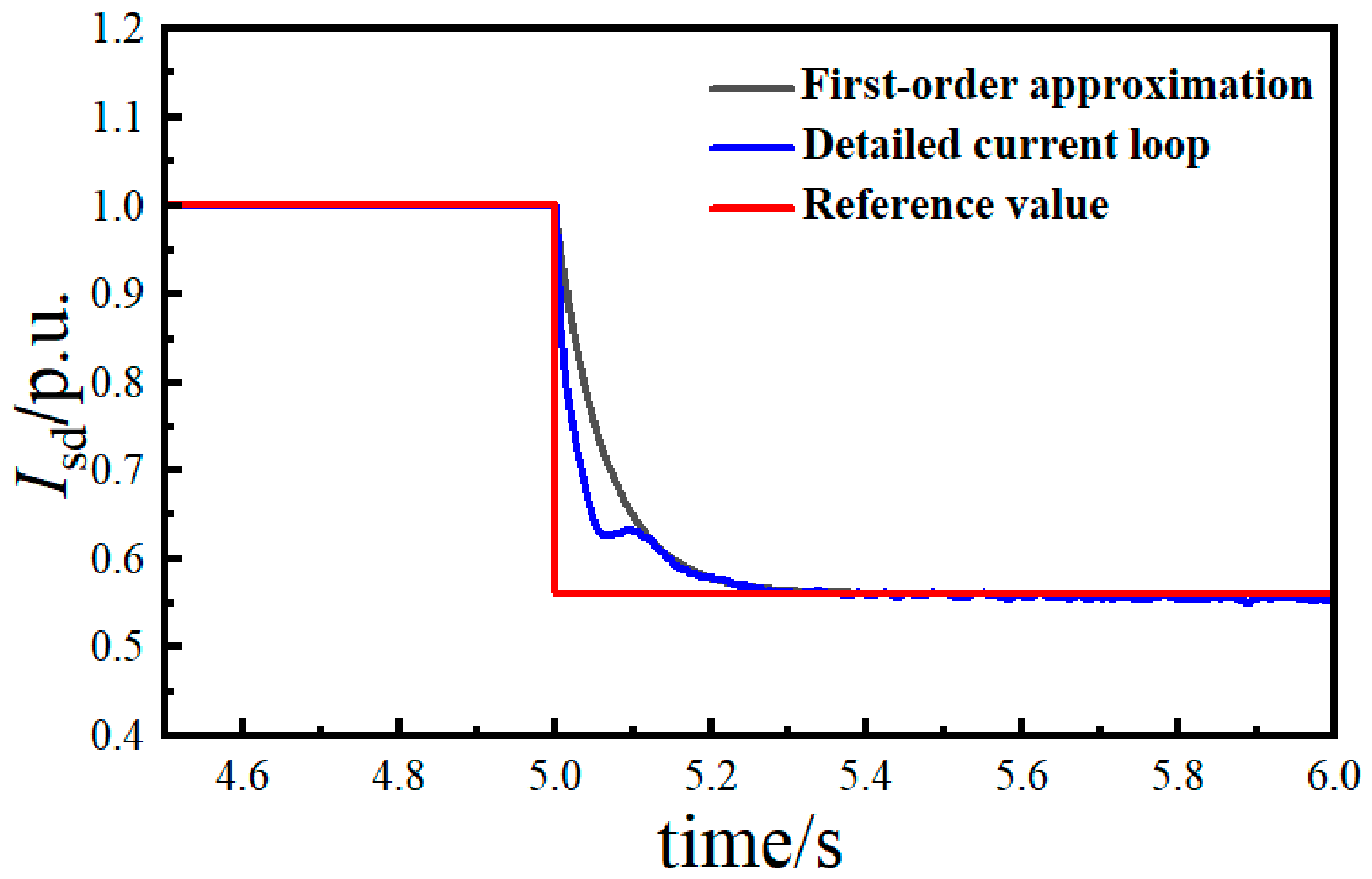
As shown in Figure A1, the response curves of the two models exhibit good overall agreement. Both models can rapidly track the reference change and eventually converge to the same steady-state value. Although a slight deviation appears during the initial transient stage, it persists only for a short period and decays rapidly, without affecting the dominant dynamic characteristics of the system. In particular, the responses of the two models almost completely overlap during the later stage of the transient process, indicating that the first-order inertial model can accurately capture the dominant dynamic behavior of the current-control inner loop.
To quantitatively evaluate the error introduced by the first-order inertial approximation, several error-related performance indices are calculated based on the responses of the detailed current-control model and the simplified model. The comparison results are summarized in Table A1.
Table A1.
Quantitative Comparison Between the Detailed Current-Control Model and the First-Order Approximation.
The maximum deviation between the detailed current-control model and the first-order approximation is approximately 0.07 p.u., and it only appears within the first 0.1 s after the disturbance. Both models converge to nearly identical steady-state values and exhibit comparable settling characteristics.
It should be noted that the objective of this study is not to investigate the detailed electromagnetic transient responses of individual electrical variables, but rather to evaluate the cumulative energy interaction among subsystems following a disturbance and its impact on transient stability. Since the response time of the current-control inner loop is on the order of milliseconds, whereas the cumulative energy index adopted in this paper is obtained by integrating the energy variation rate over a time window of several seconds, the short-duration dynamic deviations introduced by the inner-loop approximation have a negligible effect on the final cumulative energy calculation. Therefore, replacing the detailed current-control inner loop with a first-order inertial element does not significantly affect the transient stability analysis results presented in this paper.
References
- Li, K.; Huang, M.; Zha, X.; Chen, R. Review of reliability analysis methods for high-voltage direct current transmission systems. Power Syst. Prot. Control 2024, 52, 174–187. [Google Scholar] [CrossRef]
- Wei, J.; Cao, Y.; Wu, Q.; Li, C.; Huang, S.; Zhou, B. Coordinated droop control and adaptive model predictive control for enhancing HVRT and post-event recovery of large-scale wind farm. IEEE Trans. Sustain. Energy 2021, 12, 1549–1560. [Google Scholar] [CrossRef] [Scilit]
- Chen, A.; Xie, D.; Zhang, D.; Gu, C.; Wang, K. PI parameter tuning of converters for sub-synchronous interactions existing in grid-connected DFIG wind turbines. IEEE Trans. Power Electron. 2018, 34, 6345–6355. [Google Scholar] [CrossRef] [Scilit]
- Liu, H.; Sun, J. Small-signal stability analysis of offshore wind farms with LCC HVDC. In 2013 IEEE Grenoble Conference, Grenoble, France, 2013; IEEE: Piscataway, NJ, USA, 2013. [Google Scholar] [CrossRef] [Scilit]
- Zhou, C.; Wang, P. A study of temporary overvoltage at HVDC rectifier stations. In 2011 IEEE Electrical Power and Energy Conference, Winnipeg, Canada, 2011; IEEE: Piscataway, NJ, USA, 2011. [Google Scholar] [CrossRef] [Scilit]
- Huang, Y.; Li, X.; Rao, H.; Li, P.; Sun, B. Research on key issues in AC filter design for Yunguang ±800kV DC transmission project. South. Power Syst. Technol. 2010, 4, 5. [Google Scholar] [CrossRef]
- Fan, Y.; Han, M.; Liu, C.; Ding, H.; Chen, X. Coordinated control strategy for high-voltage direct current transmission of isolated hydropower grids. Power Syst. Technol. 2012, 36, 6. [Google Scholar] [CrossRef]
- Wang, X.; Taul, M.G.; Wu, H.; Liao, Y.; Blaabjerg, F.; Harnefors, L. Grid-Synchronization Stability of Converter-Based Resources—An Overview. IEEE Open J. Ind. Appl. 2020, 1, 15–134. [Google Scholar] [CrossRef] [Scilit]
- Yuan, T.; Li, F.; Yin, C. Optimization strategy of exciter control parameters for synchronous condensers to cope with DC blocking faults. Power Syst. Prot. Control 2025, 53, 125–134. [Google Scholar] [CrossRef]
- Li, J.; Tian, G.; Liu, G.; Han, X.; Qiao, S. Research on hybrid energy storage control strategy based on virtual DC motor parameter optimization. Acta Energy Solaris Sin. 2024, 45, 672–682. [Google Scholar] [CrossRef]
- Jayaudhaya, J.; Magesh, T.; Devi, G.; Isabella, L.A.; Thangavelu, R. Optimal control of FOPID controllers for PMSG wind energy conversion system using golden eagle optimization algorithm. Electr. Eng. 2025, 107, 14655–14670. [Google Scholar] [CrossRef] [Scilit]
- Xie, Y.; Tang, X.; Dong, Y.; Ma, S.; Shen, J.; Yan, J. Source-grid frequency coordinated control and parameter optimization method for UHV DC sending-end power grid with high proportion of new energy. Power Syst. Technol. 2025, 49, 263–271. [Google Scholar] [CrossRef]
- Zhu, X.; Jin, M.; Li, J.; Chen, J. Theory and simulation of supplementary damping control for unified power flow controller to mitigate subsynchronous resonance. Autom. Electr. Power Syst. 2016, 40, 44–48,97. [Google Scholar] [CrossRef]
- Sun, K.; Yao, W.; Zhou, Y.; Wen, J. Mechanism Analysis and Suppression of Medium-frequency Oscillation Based on the SISO Impedance in a PMSG-based Wind Farm When Connected to a VSC-HVDC. Proc. CSEE 2019, 39, 6908–6920+7104. [Google Scholar] [CrossRef]
- Chowdhury, M.A.; Shafiullah, G.M. SSR mitigation of series-compensated DFIG wind farms by a nonlinear damping controller using partial feedback linearization. IEEE Trans. Power Syst. 2018, 33, 2528–2538. [Google Scholar] [CrossRef] [Scilit]
- Miao, Z.; Fan, L.; Osborn, D.; Yuvarajan, S. Wind Farms with HVdc Delivery in Inertial Response and Primary Frequency Control. IEEE Trans. Energy Convers. 2024, 25, 1171–1178. [Google Scholar] [CrossRef] [Scilit]
- Sun, K.; Li, D.; Yao, W.; Zhou, Y.; Wen, J. Stability analysis and impedance reshaping control of medium-frequency oscillation in a PMSG-based wind farm connected to a VSC-HVDC. In 2022 7th Asia Conference on Power and Electrical Engineering (ACPEE), Hangzhou, China, 2022; IEEE: Piscataway, NJ, USA, 2022. [Google Scholar] [CrossRef] [Scilit]
- Liu, Z.; Tang, H.; Guo, C.; He, T. Step dead zone control strategy and optimization of DC FLC in asynchronous interconnection sending-end system with high proportion of new energy. Electr. Power Autom. Equip. 2024, 44, 116–123. [Google Scholar] [CrossRef]
- Bhukya, J.; Naidu, T.A.; Vuddanti, S.; Konstantinou, C. Co-ordinated control and parameters optimization for PSS, POD and SVC to enhance the transient stability with the integration of DFIG based wind power systems. Int. J. Emerg. Electr. Power Syst. 2022, 23, 359–379. [Google Scholar] [CrossRef] [Scilit]
- Lyu, R.; Gu, Y.; Zhong, J.; Niu, S.; Liu, Y.; Jian, L. Thermal Management and Performance Analysis of an Integrated Laminated PV-TEG Hybrid System. In 2025 International Conference on Energy Evolution and Power Engineering: Transition, Intelligence, and Autonomy (EEPE-TIA), Wuhan, China, 2025; IEEE: Piscataway, NJ, USA, 2025; pp. 1–5. [Google Scholar] [CrossRef] [Scilit]
- Arora, S.; Singh, S. Butterfly optimization algorithm: A novel approach for global optimization. Soft Comput. 2019, 23, 715–734. [Google Scholar] [CrossRef] [Scilit]
- Lyu, J.; Cai, X.; Molinas, M. Optimal design of controller parameters for improving the stability of MMC-HVDC for wind farm integration. IEEE J. Emerg. Sel. Top. Power Electron. 2018, 6, 40–53. [Google Scholar] [CrossRef] [Scilit]

Disclaimer/Publisher’s Note: The statements, opinions and data contained in all publications are solely those of the individual author(s) and contributor(s) and not of MDPI and/or the editor(s). MDPI and/or the editor(s) disclaim responsibility for any injury to people or property resulting from any ideas, methods, instructions or products referred to in the content. |
© 2026 by the authors. Licensee MDPI, Basel, Switzerland. This article is an open access article distributed under the terms and conditions of the Creative Commons Attribution (CC BY) license.