JAF-MTT: A Jerk-Aware Multi-Feature Fusion Algorithm for Maneuvering Target Tracking

Abstract

In maneuvering target tracking, traditional model-driven tracking algorithms require a predefined target motion model. The estimation accuracy degrades significantly when the actual target maneuver does not match the model assumption. Data-driven tracking algorithms can learn motion patterns directly from trajectory data, making them more robust to complex maneuvers. To improve the tracking performance in high-maneuver scenarios, this paper proposes a jerk-aware multi-feature fusion algorithm for maneuvering target tracking (JAF-MTT). The algorithm adopts jerk as the indicator of maneuver intensity. A parallel structure of convolution and multi-head self-attention is introduced to extract local and global trajectory features. These extracted features are adaptively fused in accordance with maneuver intensity. Finally, a bidirectional LSTM decodes the fused features to derive target state estimation, with the jerk adaptively modulating the gating response. Simulation results demonstrate that the performance of the proposed algorithm is better than that of the compared algorithms in high-maneuver scenarios. Moreover, the proposed algorithm maintains low tracking error under strong measurement noise.

1. Introduction

Maneuvering target tracking is essential for airspace monitoring and civil aviation surveillance. The continuous improvement of modern aerial target maneuverability has posed severe challenges to radar tracking stability. Unmanned aerial vehicles and other high-speed aerial targets often complicate radar detection through sudden maneuvers, such as sharp turns, abrupt stops, and rapid accelerations. These maneuvers lead to drastic changes in the kinematic states of the targets within a short period. Traditional tracking algorithms are prone to sustained tracking lag during target maneuvers. Therefore, developing tracking algorithms for highly maneuvering targets is of important practical value.

Traditional model-driven target tracking algorithms rely on predefined motion models to achieve target state estimation [1,2]. Refs. [3,4] adaptively adjust parameters such as the process noise and filter gain according to the maneuver intensity to improve robustness against target maneuvers. Ref. [5] estimates the target maneuver frequency to dynamically accommodate variations in maneuver intensity. Refs. [6,7] further optimize model parameters by adaptively adjusting the jerk-related noise parameters. These methods can alleviate the performance degradation caused by target maneuvers to some extent. However, a single motion model cannot accurately estimate the target state in the presence of complex maneuvers. Multiple-model (MM) methods run multiple motion models in parallel to accommodate complex target maneuvers. Among them, the interacting multiple-model (IMM) algorithm is the most widely adopted [8,9]. The IMM fuses the state estimates of all models via a probabilistic weighting strategy, enabling accurate tracking of maneuvering targets [10,11]. The traditional IMM is inherently a fixed-structure multiple-model tracking method. Once its model set is fixed, it cannot adapt to changes in target motion. When the model set is appropriately designed and well matches the true target motion, the IMM achieves satisfactory tracking performance. In practice, target motion is complex and variable. A richer set of models is often required to fully characterize the maneuver behavior. To address this issue, the variable-structure multiple-model (VSMM) approach was proposed to adaptively estimate all possible motion modes of the target [12,13,14,15,16,17]. Among these VSMM methods, the variable-structure interacting multiple-model (VSIMM) is the most representative implementation [18]. The VSIMM employs a model group switching strategy. It significantly improves the adaptability to complex maneuver patterns while effectively controlling computational complexity. However, the design of the model-switching logic and the tuning of related parameters remain highly complex [19] and rely heavily on expert experience.

The model-driven algorithms discussed above generally rely on prior assumptions about target dynamics. The estimation accuracy degrades considerably once the target maneuver pattern falls outside the predefined model set. To reduce such reliance, data-driven tracking methods have been introduced. Early studies mostly employed recurrent neural networks (RNNs) and their variants to model the temporal dependencies in trajectories [20,21]. Long short-term memory (LSTM) and gated recurrent unit (GRU) are two mainstream variants of RNN for time series modeling. The DeepMTT algorithm proposed in [22] uses a bidirectional long short-term memory (Bi-LSTM) network. It captures the temporal correlation of trajectories from both forward and backward directions to correct the estimation errors of conventional filters. This approach achieves better tracking performance than model-driven methods in weak maneuvering scenarios. Nevertheless, temporal recurrent structures exhibit limited capability in learning abrupt maneuver features. Refs. [23,24,25] introduced the attention mechanism, which adaptively weights trajectory points and highlights key temporal information at maneuver-switching moments. Refs. [23,26,27] adopt an encoder–decoder architecture and improve trajectory prediction accuracy by encoding and reconstructing trajectory sequences. Unlike recurrent and self-attention architectures, temporal convolutional network (TCN) extracts features through local receptive fields. This makes them more suitable for capturing fine-grained maneuver details [28,29].

The data-driven methods discussed above can directly learn motion patterns from trajectory data and adapt to complex maneuvers to some extent. However, in terms of feature extraction, these methods focus on either local details [20,28] or global trends [23,24], with limited attention to features and insufficient consideration given to features at the other scale. In terms of feature fusion, existing studies mostly adopt fixed weights to combine multi-scale features [24,29]. This strategy lacks the flexibility to handle complex target maneuvers effectively. The correlation between input features and target maneuvers directly determines how well the network fits the target motion. Jerk is the rate of change in acceleration. It directly quantifies maneuver intensity, making it a key feature for improving the fitting capability of the network [6,7,30]. Therefore, this paper proposes a jerk-aware multi-feature fusion algorithm for maneuvering target tracking (JAF-MTT) algorithm for highly maneuvering targets.

The main contributions of this work are summarized as follows.

(1)

A full-chain jerk-aware maneuvering target tracking framework is proposed for high-maneuver scenarios. Jerk is employed as a quantitative indicator of maneuver intensity. It is integrated into feature extraction, feature fusion, and temporal decoding to provide explicit maneuver guidance for network learning.

(2)

A jerk-modulated hybrid encoder and a bidirectional LSTM decoder are designed. The encoder adopts a dual-branch parallel structure. The left branch uses dilated causal convolution to extract local maneuver features, while the right branch adopts multi-head self-attention with jerk modulating the query vector, enabling the model to focus global attention on high-maneuver periods. In the decoder, jerk features are incorporated into the gating units of the bidirectional LSTM, and the gates respond to maneuver intensity accordingly.

(3)

We propose an adaptive weighted fusion mechanism based on jerk maneuver intensity. The mechanism replaces traditional fixed fusion strategies. Instead, it dynamically computes the fusion weights of local and global features according to the normalized jerk value. In this way, local features are emphasized during high-maneuver motions, and global features dominate during smooth motion.

The rest of the paper is arranged as follows. Section 2 presents the problem formulation. Section 3 describes the proposed JAF-MTT algorithm in detail. Section 4 validates the tracking performance through comparative experiments, ablation studies, and noise robustness tests. Section 5 concludes the paper and points to future research directions.

2. Problem Description

This section formulates the maneuvering target tracking problem in a two-dimensional plane. The tracking system adopts a two-dimensional passive radar as the observation sensor, which outputs slant range and azimuth measurements in polar form at a fixed sampling interval $T=1 \mathrm{s}$. Both the range and azimuth measurement noise follow zero-mean Gaussian distributions, with standard deviations ${\sigma }_r=10 \mathrm{m}$ and ${\sigma }_{\theta }={0.1}^{°}$, respectively.

At time step $k$, the target state vector is defined as

$${\mathit{X}}_k={[x_k, y_k, {\dot{x}}_k, {\dot{y}}_k]}^{\mathrm{T}},$$

(1)

where $x_k$ and $y_k$ denote the target position in Cartesian coordinates, and ${\dot{x}}_k$ and ${\dot{y}}_k$ are the corresponding velocity components.

The target motion follows the discrete-time state transition equation

$${\mathit{X}}_{k+1}={\mathit{F}}_k{\mathit{X}}_k+{\mathit{w}}_k,$$

(2)

where ${\mathit{F}}_k$ denotes the state transition matrix determined by the current motion mode, and ${\mathit{w}}_k$ represents the process noise.

The measurement equation of the radar in polar coordinates is expressed as

$${\mathit{Z}}_k=\mathit{h}({\mathit{X}}_k)+{\mathit{v}}_k,$$

(3)

where ${\mathit{Z}}_k={[{\rho }_k, {\theta }_k]}^{\mathrm{T}}$ is the noisy measurement vector, ${\rho }_k$ is the range, ${\theta }_k$ is the azimuth, $\mathit{h}(\cdot )$ is the nonlinear measurement mapping function, and ${\mathit{v}}_k$ is the measurement noise.

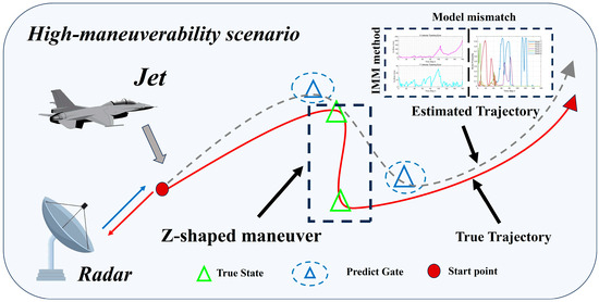
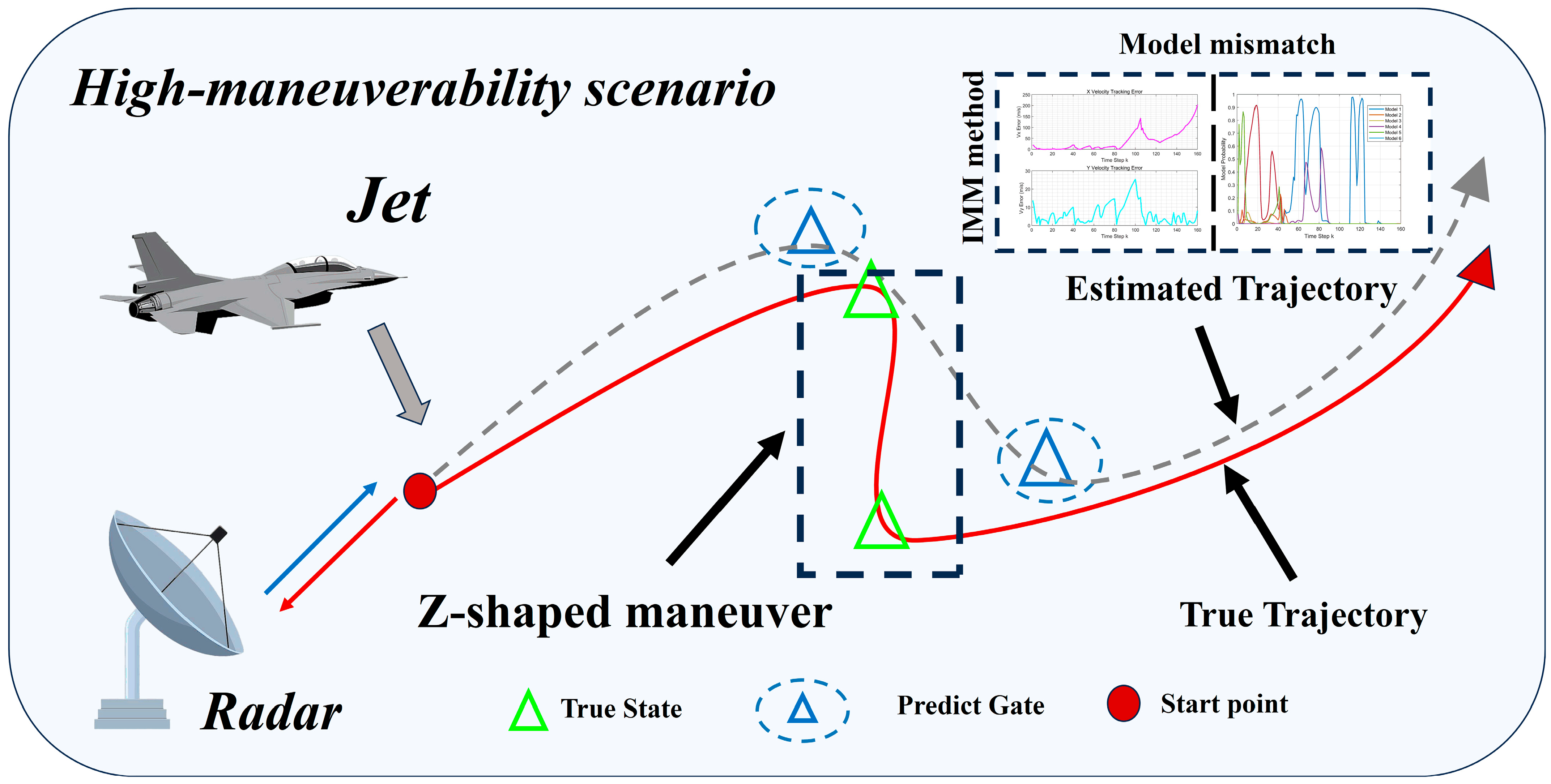
The task of maneuvering target tracking is to estimate the true target state sequence $\mathit{X}=\left\{{\mathit{X}}_1,\right.\cdot \cdot \cdot \left.{\mathit{X}}_k\right\}$ from the noisy measurement sequence $\mathit{Z}=\left\{{\mathit{Z}}_1,\right.\cdot \cdot \cdot \left.{\mathit{Z}}_k\right\}$. In the above model, the process noise covariance indicates the degree to which the actual motion deviates from the assumed model. During stationary motion, this deviation is minor, and the covariance stays small. However, during high maneuvers, rapid state changes cause a clear mismatch with the assumed model, and the covariance increases sharply. This model mismatch problem is depicted in Figure 1.

Figure 1. Illustration of model mismatch in a high-maneuver scenario.

In the figure, the red solid curve traces the true trajectory, and the gray dashed curve marks the estimated one. The trajectory contains two sharp turns in opposite directions. During maneuver-switching periods, a clear deviation appears between the prediction and the true target state. This mismatch prevents the tracking algorithm from capturing the target’s abrupt maneuvers in time, causing the estimated trajectory to lag behind and degrading tracking performance.

3. The Proposed Method

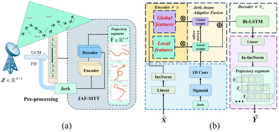
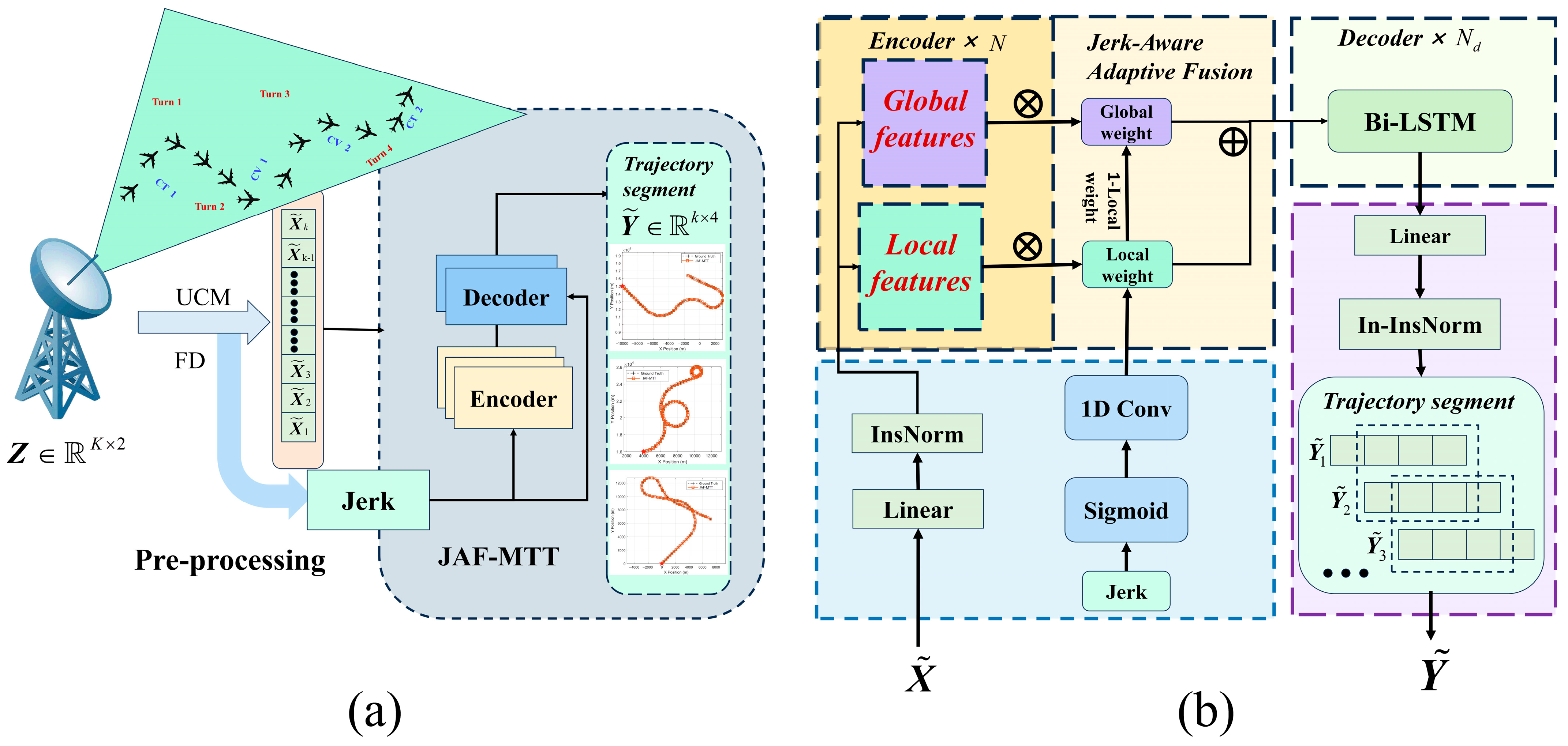
This section describes the architecture of the proposed JAF-MTT algorithm. Its overall workflow is illustrated in Figure 2. The algorithm is built around a data preprocessing module and a fully trainable trajectory mapping network. It operates on the radar polar measurement sequence $\mathit{Z}\in {\mathsf{ℝ}}^{K\times 2}$ to produce the state estimate of the true target trajectory $\tilde{\mathit{Y}}\in {\mathsf{ℝ}}^{k\times 4}$.

Figure 2. Framework of the proposed JAF-MTT algorithm. (a) Schematic of the JAF-MTT tracking framework. (b) Network architecture of the JAF-MTT.

Figure 2a illustrates the complete maneuvering target tracking flow of JAF-MTT. The raw radar polar measurements are first converted to Cartesian position components via the unbiased converted measurement (UCM) technique. Based on the converted position sequence, the velocity, acceleration, and jerk components are computed using the finite difference method. These components are then concatenated to form the complete measurement trajectory sequence $\tilde{\mathit{X}}\in {\mathsf{ℝ}}^{k\times 8}$, where each frame consists of eight motion features covering the position, velocity, acceleration, and jerk in both directions.

Figure 2b presents the network architecture of JAF-MTT. The observed trajectory sequence first undergoes instance normalization (InsNorm) and linear dimension lifting. These operations project the raw input into a higher-dimensional representation. The processed features are then fed into an encoding module composed of stacked hybrid encoders. Each encoder layer employs a dual-branch parallel structure. The dilated causal convolution branch extracts local features, and the multi-head self-attention branch captures global features. The jerk-aware adaptive fusion unit subsequently fuses the two-branch outputs into integrated features. These fused features are passed to a decoding module built with stacked decoders. Each decoder applies a bidirectional LSTM structure. Jerk features are injected into the gating units to dynamically adjust state updates according to maneuver intensity. The decoder output then undergoes linear dimension reduction and inverse instance normalization (inv-InsNorm). Finally, a sliding window trajectory reconstruction strategy produces a complete and smooth target state estimation sequence.

3.1. Data Preprocessing

The raw measurement acquired by the radar at each time step consists of the slant range and azimuth angle in polar coordinates, expressed as

$${\mathit{Z}}_k={\left[{\rho }_k, {\theta }_k\right]}^{\mathrm{T}},$$

(4)

where ${\rho }_k$ and ${\theta }_k$ denote the noisy slant range and azimuth observations, respectively. Both are corrupted by zero-mean Gaussian noise added to the true values. The conventional trigonometric coordinate conversion introduces systematic mean bias due to the nonlinear coupling of observation noise. To eliminate this bias, UCM is adopted, which incorporates an azimuth noise compensation factor to produce unbiased Cartesian position components as follows

$$\begin{array}{l}{\tilde{x}}_k^{ub}={\alpha }_k\cdot {\tilde{r}}_k\cos {\tilde{\theta }}_k,\\ {\tilde{y}}_k^{ub}={\alpha }_k\cdot {\tilde{r}}_k\sin {\tilde{\theta }}_k,\end{array}$$

(5)

where ${\alpha }_k=\exp ({\sigma }_{\theta }^2/2)$ is the azimuth compensation factor, and ${\sigma }_{\theta }$ is the azimuth measurement uncertainty parameter.

To mitigate severe noise amplification induced by high-order successive finite differentiation on noisy unbiased UCM coordinates, a three-point moving average pre-smoothing is performed on raw UCM outputs ${\tilde{x}}_k^{ub},{\tilde{y}}_k^{ub}$ prior to difference calculation. The smoothed position variables ${\overline{x}}_k^{ub},{\overline{y}}_k^{ub}$ are defined as

$$\begin{array}{l}{\overline{x}}_k^{ub}={\displaystyle \frac{{\tilde{x}}_{k-1}^{ub}+{\tilde{x}}_k^{ub}+{\tilde{x}}_{k+1}^{ub}}{3}},\\ {\overline{y}}_k^{ub}={\displaystyle \frac{{\tilde{y}}_{k-1}^{ub}+{\tilde{y}}_k^{ub}+{\tilde{y}}_{k+1}^{ub}}{3}},\end{array}$$

(6)

For boundary endpoints without forward or backward neighboring sampling points, the boundary coordinate is duplicated to complete the smoothing operation. All subsequent velocity, acceleration and jerk kinematic components are derived from smoothed ${\overline{x}}_k^{ub},{\overline{y}}_k^{ub}$, rather than original unprocessed UCM position ${\tilde{x}}_k^{ub},{\tilde{y}}_k^{ub}$.

Based on the smoothed unbiased position sequences ${\overline{x}}_k^{ub}$ and ${\overline{y}}_k^{ub}$, we compute the kinematic states along both the x and y axes using the finite difference method, with a fixed sampling period $T$, as detailed below.

$$\begin{array}{l}{\dot{\tilde{x}}}_k={\displaystyle \frac{{\overline{x}}_k^{ub}-{\overline{x}}_{k-1}^{ub}}{T}},\hspace{1em}{\dot{\tilde{y}}}_k={\displaystyle \frac{{\overline{y}}_k^{ub}-{\overline{y}}_{k-1}^{ub}}{T}},\\ {\ddot{\tilde{x}}}_k={\displaystyle \frac{{\dot{\tilde{x}}}_k-{\dot{\tilde{x}}}_{k-1}}{T}},\hspace{1em}{\ddot{\tilde{y}}}_k={\displaystyle \frac{{\dot{\tilde{y}}}_k-{\dot{\tilde{y}}}_{k-1}}{T}},\\ {\stackrel{⃛}{\tilde{x}}}_k={\displaystyle \frac{{\ddot{\tilde{x}}}_k-{\ddot{\tilde{x}}}_{k-1}}{T}},\hspace{1em}{\stackrel{⃛}{\tilde{y}}}_k={\displaystyle \frac{{\ddot{\tilde{y}}}_k-{\ddot{\tilde{y}}}_{k-1}}{T}}, \end{array}$$

(7)

where ${\dot{\tilde{x}}}_k$, ${\dot{\tilde{y}}}_k$ denote the velocity, ${\ddot{\tilde{x}}}_k$, ${\ddot{\tilde{y}}}_k$ are the acceleration, and ${\stackrel{⃛}{\tilde{x}}}_k$, ${\stackrel{⃛}{\tilde{y}}}_k$ are the jerk. Stacking the smoothed unbiased positions together with the above kinematic components yields an 8-dimensional feature vector

$${\tilde{\mathit{X}}}_k={\left[{\overline{x}}_k^{ub},{\overline{y}}_k^{ub},{\dot{\tilde{x}}}_k,{\dot{\tilde{y}}}_k,{\ddot{\tilde{x}}}_k,{\ddot{\tilde{y}}}_k,{\stackrel{⃛}{\tilde{x}}}_k,{\stackrel{⃛}{\tilde{y}}}_k\right]}^{\mathrm{T}},$$

(8)

The feature vectors at all time steps form the complete observation trajectory sequence $\tilde{\mathit{X}}=\left\{{\tilde{\mathit{X}}}_1,{\tilde{\mathit{X}}}_2,\dots ,{\tilde{\mathit{X}}}_k\right\}\in {\mathsf{ℝ}}^{k\times 8}$, which serves as the input to the subsequent feature mapping network. The frame-level maneuver intensity $J_k$ is defined based on the two-dimensional jerk components as

$$J_k=\sqrt{{\stackrel{⃛}{\tilde{x}}}_k^2+{\stackrel{⃛}{\tilde{y}}}_k^2}.$$

(9)

The maneuver intensity is then normalized to obtain the maneuver weight $w_k$:

$$w_k=\sigma (J_k)={\displaystyle \frac{1}{1+\exp (-J_k)}},$$

(10)

where $J_k$ denotes the Sigmoid activation function. A larger $J_k$ corresponds to stronger maneuver abruptness, and $w_k$ approaches 1. When the target moves smoothly, $J_k$ is small and $w_k$ approaches 0.

3.2. Convolutional-Multi-Head Self-Attention Hybrid Encoder

A window of fixed size $L$ slides over the observation trajectory with stride $S$. Window $m$ starts at time step $k_m$, and its features are

$${\tilde{\mathit{X}}}_m={\left[{\tilde{\mathit{X}}}_{k_m},{\tilde{\mathit{X}}}_{k_m+1},\dots ,{\tilde{\mathit{X}}}_{k_m+L-1}\right]}^{\top }\in {\mathsf{ℝ}}^{L\times 8}.$$

(11)

For segments at the trajectory beginning whose length is less than $L$, the missing frames are filled by repeating the first frame. Since the eight motion components span different numerical ranges and units, instance normalization and linear projection are performed before feeding them into the network

$$\begin{array}{l}{\widehat{\mathit{X}}}_m={\displaystyle \frac{{\tilde{\mathit{X}}}_m-{\mathit{\mu }}_m}{\sqrt{{\mathit{\sigma }}_m^2+\epsilon }}},\\ {\mathit{X}}_m^{in}={\widehat{\mathit{X}}}_m\mathit{W}+\mathit{b},\end{array}$$

(12)

where ${\mathit{\mu }}_m\in {\mathsf{ℝ}}^8$ and ${\mathit{\sigma }}_m\in {\mathsf{ℝ}}^8$ are the per-channel mean and standard deviation of sliding window $m$, $\epsilon ={10}^{-8}$. $W$ is a learnable weight matrix, and $\mathit{b}$ is a bias vector. The mean and standard deviation are computed as

$$\begin{array}{l}{\mathit{\mu }}_{m,d}={\displaystyle \frac{1}{L}}{\displaystyle \sum _{k=1}^L{\tilde{\mathit{X}}}_{m,k,d}},\\ {\mathit{\sigma }}_{m,d}=\sqrt{{\displaystyle \frac{1}{L}}{\displaystyle \sum _{k=1}^L{\left({\tilde{\mathit{X}}}_{m,k,d}-{\mathit{\mu }}_{m,d}\right)}^2}},\end{array}$$

(13)

where $d$ denotes the channel of the 8-dimensional kinematic features.

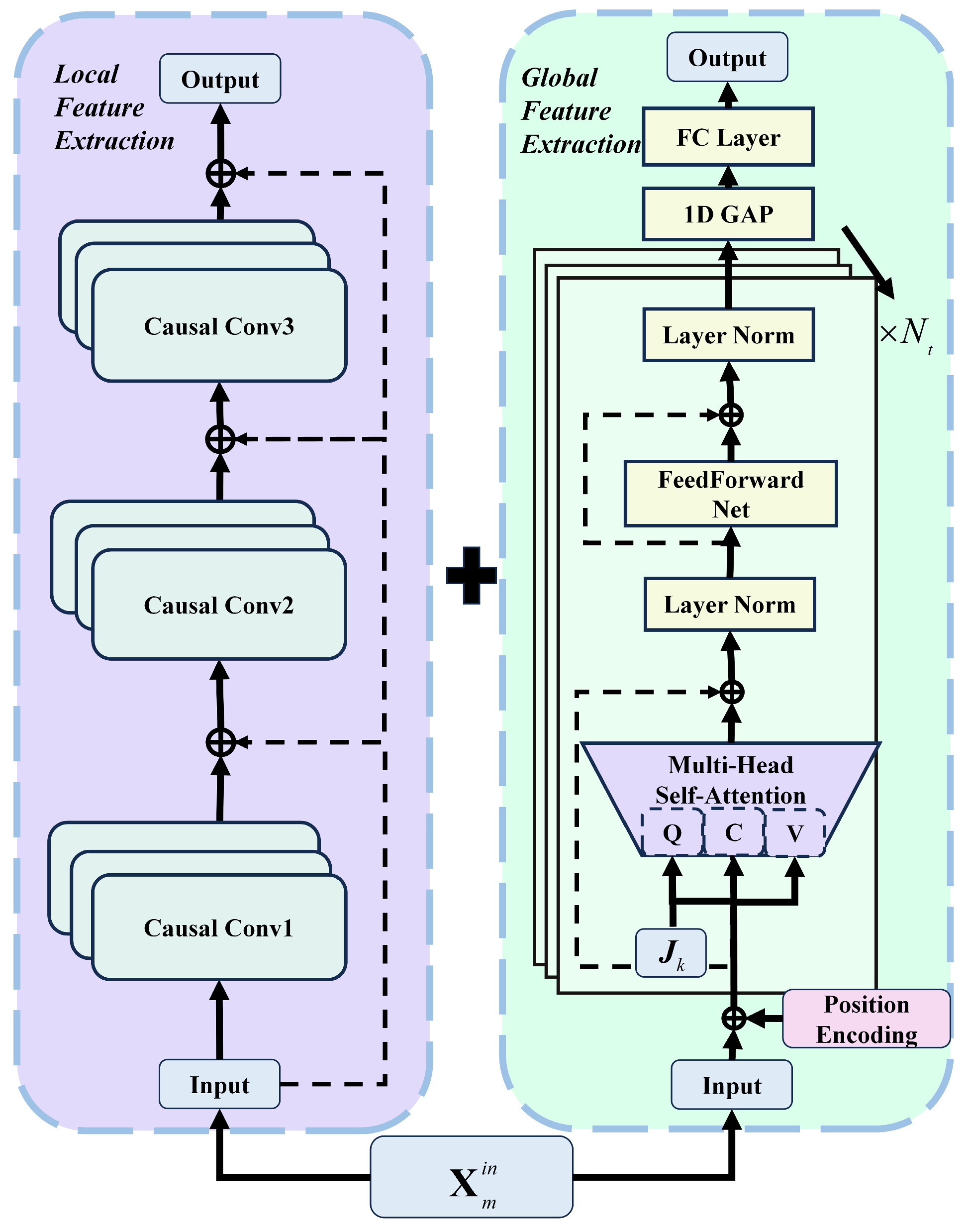
The processed features are fed into the hybrid encoder. Its dual-branch parallel structure is illustrated in Figure 3. The left branch consists of a dilated causal residual convolutional network for capturing local transient maneuvers. The right branch employs a jerk-modulated multi-head self-attention encoder for modeling global temporal dependencies.

Figure 3. Dual-branch feature extraction structure of the hybrid encoder.

The left branch consists of $N_c$ stacked residual blocks. The convolution kernel size is $K$, and the dilation rate increases exponentially with the layer index as $d_b=2^{b-1}$. Let ${\mathit{R}}_m^0={\mathit{X}}_m^{\mathrm{in}}$ be the input. The forward propagation of block $b$ is

$${\mathit{R}}_m^b=\mathrm{Dropout}\left(\mathrm{ReLU}\left(\mathrm{BN}\left({\mathrm{CausalConv}}_{K,d_b}\left({\mathit{R}}_m^{(b-1)}\right)\right)\right)\right)+{\mathit{R}}_m^{(b-1)},$$

(14)

where $\mathrm{CausalConv}$ denotes the causal convolution whose kernel size is $K$ and dilation rate is $d_b$, BN is batch normalization, and the dropout rate is set to 0.2. The residual connection mitigates gradient vanishing. After $N_c$ blocks, the branch outputs ${\mathit{X}}_m^{local}={\mathit{R}}_m^{N_t}\in {\mathsf{ℝ}}^{L\times D}$.

The right branch consists of $N_t$ layers of multi-head self-attention encoders. Each layer has a self-attention module with multiple heads and a position-wise feed-forward network, with each followed by a residual connection and layer normalization (LN). To enhance the network’s perception of high-maneuver periods, the right branch introduces the jerk feature into the computation of the attention query vector. This allows the attention weights to adjust adaptively according to the maneuver intensity. Furthermore, because the self-attention mechanism is insensitive to sequence order, the right branch adds a sinusoidal–cosinusoidal absolute position encoding to the input features. For window sequence length $L$, the position encoding $\mathit{P}\in {\mathsf{ℝ}}^{L\times D}$ is defined as

$$\begin{array}{l}\mathit{P}[k,2i]=\sin \left({\displaystyle \frac{k}{{10000}^{2i/D}}}\right),\\ \mathit{P}[k,2i+1]=\cos \left({\displaystyle \frac{k}{{10000}^{2i/D}}}\right),\end{array}$$

(15)

where $i=0,1,\dots ,D/2-1$. The initial global feature with position information is

$${\mathit{E}}_m^0={\mathit{X}}_m^{\mathrm{in}}+\mathit{P}.$$

(16)

The multi-head self-attention uses $H$ heads with per-head dimension $d_k=D/H$. For head $i$, the query vector is modulated by the jerk feature as

$${\tilde{\mathit{Q}}}_{m,i}={\mathit{E}}_m^{j-1}\cdot {\mathit{W}}_i^{\mathrm{Q}}+{\mathit{J}}_k^m\cdot {({\mathit{w}}_k^i)}^{\mathrm{T}},$$

(17)

where ${\mathit{w}}_k^i\in {\mathsf{ℝ}}^{2\times d_k}$ is the Jerk projection matrix for head $i$, ${\mathit{E}}_m^{j-1}$ is the input to encoder layer $j$, and ${\mathit{W}}_i^{\mathrm{Q}}\in {\mathsf{ℝ}}^{D\times d_k}$ is the query projection matrix. The output of head $i$ is

$$\mathit{h}\mathit{e}\mathit{a}{\mathit{d}}_{m,i}=\mathrm{softmax}\left({\displaystyle \frac{{\mathit{Q}}_{m,i}\cdot {({\mathit{K}}_{m,i})}^{\top }}{\sqrt{d_k}}}\right)\cdot {\mathit{V}}_{m,i}.$$

(18)

The outputs of all heads are concatenated and linearly projected. The computation of encoder layer $j$ is

$$\begin{array}{l}{\mathit{F}}_m^j=\mathrm{LN}\left(\mathit{MultiHead}\left({\mathit{E}}_m^{j-1}\right)+{\mathit{E}}_m^{j-1}\right),\\ {\mathit{E}}_m^j=\mathrm{LN}\left(\mathrm{FFN}\left({\mathit{F}}_m^j\right)+{\mathit{F}}_m^j\right),\end{array}$$

(19)

where $\mathrm{FFN}$ denotes a feed-forward network with two linear transformations and $\mathrm{Re}\mathrm{LU}$ activation. After $N_t$ layers, the branch outputs ${\mathit{X}}_m^{\mathrm{global}}={\mathit{E}}_m^N\in {\mathsf{ℝ}}^{L\times D}$.

The fused feature is computed as the weighted sum of the two branch outputs:

$${\mathit{X}}_m^{\mathrm{fusion}}={\mathit{W}}_m^{\mathrm{local}}\odot {\mathit{X}}_m^{\mathrm{local}}+{\mathit{W}}_m^{\mathrm{global}}\odot {\mathit{X}}_m^{\mathrm{global}},$$

(20)

where ${\mathit{X}}_m^{\mathrm{local}}$ and ${\mathit{X}}_m^{\mathrm{global}}$ are the outputs of the left and right branches, $\odot$ denotes element-wise multiplication, and the fusion weight matrices are obtained by broadcasting the jerk maneuver weight sequence ${\mathit{w}}_k^m={[w_1^m,w_2^m,\dots ,w_L^m]}^{\mathrm{T}}\in {\mathsf{ℝ}}^L$ as

$$\begin{array}{l}{\mathit{W}}_m^{\mathrm{local}}={\mathit{w}}_k^m\otimes {\mathbf{1}}_D^{\mathrm{T}},\\ {\mathit{W}}_m^{\mathrm{global}}=({\mathbf{1}}_L-{\mathit{w}}_k^m)\otimes {\mathbf{1}}_D^{\mathrm{T}},\end{array}$$

(21)

where ${\mathbf{1}}_L\in {\mathsf{ℝ}}^L$ and ${\mathbf{1}}_D\in {\mathsf{ℝ}}^D$ are all-ones vectors, and $\otimes$ denotes the outer product.

3.3. Jerk-Modulated Bidirectional LSTM Decoder

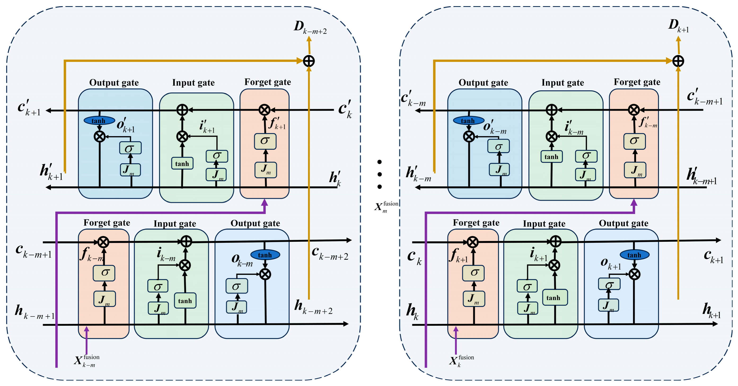
This section uses a jerk-modulated BiLSTM to decode the sequence and generate the final state estimate. The decoder stacks several BiLSTM layers. Each layer contains two independent LSTM branches, namely a forward branch and a backward branch. The forward branch handles the sequence in temporal order, and the backward branch handles it in reverse temporal order. The structure of the jerk-modulated LSTM unit is illustrated in Figure 4.

Figure 4. Jerk-modulated bidirectional long short-term memory decoder unit structure.

At time step $k$, the forward LSTM in layer $n$ contains a forget gate ${\mathit{f}}_{k,n}$, an input gate ${\mathit{i}}_{k,n}$, an output gate ${\mathit{o}}_{k,n}$, a candidate cell state ${\tilde{\mathit{c}}}_{k,n}$, a cell state ${\mathit{c}}_{k,n}$, and a hidden state ${\mathit{h}}_{k,n}$. The jerk feature ${\mathit{J}}_m$ is incorporated into each gate computation to enhance the responsiveness to high maneuvers. The update equations of the forward LSTM in layer $n$ are

$$\begin{array}{l}{\mathit{i}}_{k,n}=\sigma ({\mathit{X}}_{m,k}^{\mathrm{fusion}}{\mathit{W}}_n^{ix}+{\mathit{h}}_{k-1,n}{\mathit{W}}_n^{ih}+{\mathit{J}}_k^m{\mathit{W}}_n^{iJ}+{\mathit{b}}_n^i),\\ {\mathit{f}}_{k,n}=\sigma ({\mathit{X}}_{m,k}^{\mathrm{fusion}}{\mathit{W}}_n^{fx}+{\mathit{h}}_{k-1,n}{\mathit{W}}_n^{fh}+{\mathit{J}}_k^m{\mathit{W}}_n^{fJ}+{\mathit{b}}_n^f),\\ {\mathit{o}}_{k,n}=\sigma ({\mathit{X}}_{m,k}^{\mathrm{fusion}}{\mathit{W}}_n^{ox}+{\mathit{h}}_{k-1,n}{\mathit{W}}_n^{oh}+{\mathit{J}}_k^m{\mathit{W}}_n^{oj}+{\mathit{b}}_n^o),\\ {\tilde{\mathit{c}}}_{k,n}=\tanh ({\mathit{X}}_{m,k}^{\mathrm{fusion}}{\mathit{W}}_n^{cx}+{\mathit{h}}_{k-1,n}{\mathit{W}}_n^{ch}+{\mathit{b}}_n^c),\\ {\mathit{c}}_{k,n}={\mathit{f}}_{k,n}\odot {\mathit{c}}_{k-1,n}+{\mathit{i}}_{k,n}\odot {\tilde{\mathit{c}}}_{k,n},\\ {\mathit{h}}_{k,n}={\mathit{o}}_{k,n}\odot \tanh ({\mathit{c}}_{k,n}),\end{array}$$

(22)

where $\sigma (\cdot )$ and $\tanh (\cdot )$ are the Sigmoid and hyperbolic tangent activation functions. ${\mathit{W}}_n^{fx}$, ${\mathit{W}}_n^{fh}$, and ${\mathit{W}}_n^{fj}$ are the weight matrices for the input feature, hidden state, and jerk feature, respectively. ${\mathit{b}}_n^f$ denotes the bias term. ${\mathit{h}}_{m,k-1,n}$ is the hidden state of the forward LSTM in layer $n$ at time $k-1$, and ${\mathit{J}}_k^m$ is the jerk feature vector at time step $k$ within the window. All weight matrices and bias terms in the gates are learnable parameters. The jerk feature injection enables the gate values to adapt dynamically to maneuver intensity. During high-maneuver periods, the forget gate weakens and the input gate strengthens, allowing the network to focus on the current abrupt change. During smooth periods, the reverse occurs, effectively suppressing noise.

The backward LSTM adopts the same structure and processes the sequence in reverse order, yielding the hidden state ${{\mathit{h}}^{\prime }}_{k,n}$. The forward and backward hidden states are summed to produce the output of layer $n$

$${\mathit{D}}_{m,k,n}={\mathit{h}}_{k,n}+{{\mathit{h}}^{\prime }}_{k,n}.$$

(23)

After $N_d$ stacked layers, a jerk-weighted residual connection is introduced to prevent high-maneuver features from decaying in deep layers. The final decoded feature at time step $k$ is

$${\mathit{Y}}_m^D={\mathit{D}}_{m,k,N_d}+{\mathit{w}}_k^m\odot {\mathit{D}}_{m,k,1},$$

(24)

where ${\mathit{D}}_{m,k,N_d}$ and ${\mathit{D}}_{m,k,1}$ denote the outputs of the deepest and the first decoder layers, respectively. ${\mathit{w}}_k^m$ represents the jerk maneuver weight at time step $k$.

The decoded feature is then linearly projected to the target state dimension and restored to the original physical scale via inverse instance normalization

$${\tilde{\mathit{Y}}}_m={\mathit{Y}}_m^{out}\odot {\mathit{\sigma }}_m^{1:4}+{\mathit{\mu }}_m^{1:4},$$

(25)

where ${\mathit{\mu }}_m^{1:4}$ and ${\mathit{\sigma }}_m^{1:4}$ are the first four components of ${\mathit{\mu }}_m$ and ${\mathit{\sigma }}_m$ corresponding to the position and velocity channels, and $\odot$ denotes element-wise multiplication. The final output ${\tilde{\mathit{Y}}}_m\in {\mathsf{ℝ}}^{L\times 4}$ is the state estimate within the sliding window.

3.4. Trajectory Reconstruction

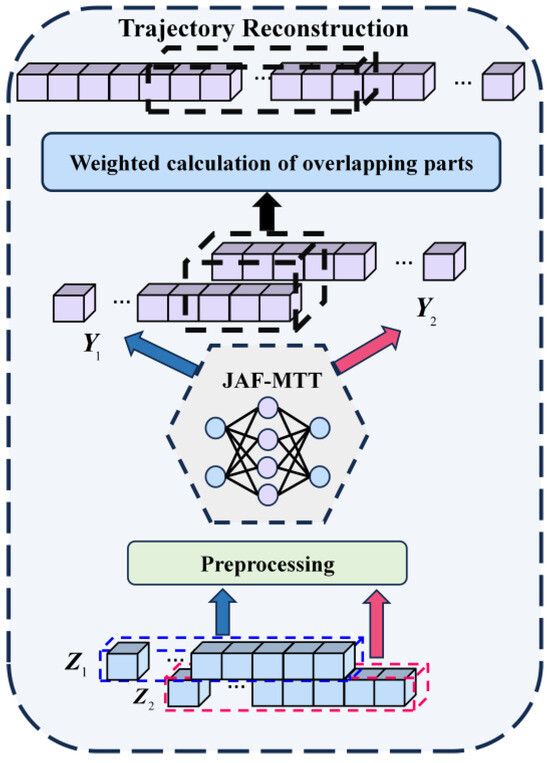
The state estimates from each sliding window are combined to form the complete trajectory through a reconstruction pipeline, which is illustrated in Figure 5. Each window is preprocessed and then fed into the JAF-MTT network, yielding the corresponding state estimate ${\tilde{\mathit{Y}}}_m\in {\mathsf{ℝ}}^{L\times 4}$.

Figure 5. JAF-MTT trajectory reconstruction pipeline.

To suppress boundary artifacts caused by window segmentation, a Hann-window weight sequence is generated for each window:

$${\mathit{w}}_{m,k}^{\mathrm{Hann}}=0.5\cdot \left(1-\cos \left({\displaystyle \frac{2\pi k}{L+1}}\right)\right),$$

(26)

where ${\mathit{w}}_{m,k}^{\mathrm{Hann}}$ is the Hann-window weight at time step $k$ within window $m$. This weight approaches 0 at both ends of the window and approaches 1 at the center, thus reducing the influence of boundary estimates. The dynamic fusion weight is then constructed as

$${\mathit{w}}_{m,k}^{\mathrm{fus}}={\mathit{w}}_{m,k}^{\mathrm{Hann}}\cdot {\mathit{w}}_k^m.$$

(27)

For two adjacent windows $m$ and $m+1$, a frame in the overlapping region has index $p=S+i$ in window $m$ and index $q=i$ in window $m+1$. The state estimates in the overlapping region are fused using the dynamic weights

$${\tilde{\mathit{Y}}}_m^{\mathrm{fus}}={\displaystyle \frac{{\mathit{w}}_{m,p}^{\mathrm{fusion}}\cdot {\tilde{\mathit{Y}}}_m[p,:]+{\mathit{w}}_{m+1,q}^{\mathrm{fusion}}\cdot {\tilde{\mathit{Y}}}_{m+1}[q,:]}{{\mathit{w}}_{m,p}^{\mathrm{fus}}+{\mathit{w}}_{m+1,q}^{\mathrm{fus}}}},$$

(28)

where ${\tilde{\mathit{Y}}}_m[p,:]$ is the state estimate at frame $p$ in window $m$, and ${\tilde{\mathit{Y}}}_{m+1}[q,:]$ is the state estimate at frame $q$ in window $m+1$.

The fusion results of all overlapping frames are arranged in time order to form the fused state sequence of the overlapping region ${\tilde{\mathit{Y}}}_m^{\mathrm{fus}}\in {\mathsf{ℝ}}^{(L-S)\times 4}$. The non-overlapping part of each window is directly retained as ${\tilde{\mathit{Y}}}_{m,\mathrm{non}}\in {\mathsf{ℝ}}^{S\times 4}$. Finally, the non-overlapping segments and the fused overlapping segments are alternately concatenated in time order to obtain the complete trajectory:

$$\tilde{\mathit{Y}}=\left[{\tilde{\mathit{Y}}}_{1,\mathrm{non}},{\tilde{\mathit{Y}}}_1^{\mathrm{fus}},{\tilde{\mathit{Y}}}_{2,\mathrm{non}},{\tilde{\mathit{Y}}}_2^{\mathrm{fus}},\dots ,{\tilde{\mathit{Y}}}_{M,\mathrm{non}}\right],$$

(29)

where $\tilde{\mathit{Y}}\in {\mathsf{ℝ}}^{K\times 4}$ is the final estimate, containing the 4-dimensional position and velocity state estimates for the entire duration.

4. Simulation

In this section, we evaluate the tracking performance of the proposed JAF-MTT algorithm. The position RMSE and velocity RMSE are adopted as evaluation metrics. In Monte Carlo run $i$ at time step $k$, $({\tilde{x}}_{k,i},{\tilde{y}}_{k,i})$ and $(x_{k,i},y_{k,i})$ denote the estimated and true positions, respectively. $({\tilde{\dot{x}}}_{k,i},{\tilde{\dot{y}}}_{k,i})$ and $({\dot{x}}_{k,i},{\dot{y}}_{k,i})$ denote the estimated and true velocities, respectively. The two metrics are defined as

$$\begin{array}{l}{\mathrm{RMSE}}_{\mathrm{pos}}=\sqrt{{\displaystyle \frac{1}{N\cdot K}}{\displaystyle \sum _{i=1}^N{\displaystyle \sum _{k=1}^K\left[{\left({\tilde{x}}_{k,i}-x_{k,i}\right)}^2+{\left({\tilde{y}}_{k,i}-y_{k,i}\right)}^2\right]}}},\\ {\mathrm{RMSE}}_{\mathrm{vel}}=\sqrt{{\displaystyle \frac{1}{N\cdot K}}{\displaystyle \sum _{i=1}^N{\displaystyle \sum _{k=1}^K\left[{\left({\tilde{\dot{x}}}_{k,i}-{\dot{x}}_{k,i}\right)}^2+{\left({\tilde{\dot{y}}}_{k,i}-{\dot{y}}_{k,i}\right)}^2\right]}}},\end{array}$$

(30)

where $N=100$ denotes the number of Monte Carlo runs, and $K$ denotes the total number of time steps per trajectory.

4.1. Dataset Construction

The simulation dataset is constructed based on a high-maneuver target tracking scenario in a 2D plane. Target motion states are generated using the state space model (SSM), and all motion patterns consist of constant velocity (CV) and constant turn (CT) maneuvers. The initial target state is randomly initialized within the radar detection range, and the initial heading angle follows a uniform distribution. Each trajectory contains multiple maneuver mode switches, with the turn rate uniformly sampled from a preset range.

The generated data are partitioned into three disjoint subsets for training, validation, and testing. All subsets follow the same data distribution. The full parameter configuration is provided in Table 1.

Table 1. Parameter settings for dataset generation.

Parameter	Value/Range
Radar sampling interval $T$	$T=0.1 \mathrm{s}$
Single trajectory duration	$100 \mathrm{s}$
Target initial velocity	$[50 \mathrm{m}/\mathrm{s},400 \mathrm{m}/\mathrm{s}]$
Number of maneuver switches per trajectory	$[2,6]$
Target turn rate $\omega$	$[-{15}^{°}/\mathrm{s},{15}^{°}/\mathrm{s}]$
$\mathrm{Standard} \mathrm{deviation} \mathrm{of} \mathrm{range} \mathrm{noise} {\sigma }_{\rho }$	$[8 \mathrm{m},13 \mathrm{m}]$
$\mathrm{Standard} \mathrm{deviation} \mathrm{of} \mathrm{azimuth} \mathrm{noise} {\sigma }_{\theta }$	$[{0.4}^{°},{0.6}^{°}]$
Training set size	$50000$
Validation set size	$1000$
Test set size	$1000$

4.2. Parameter Selection

The hybrid encoder and the temporal decoder contain several parameters that directly affect tracking performance. This section determines the optimal configuration using the control variable method. For this analysis, a high-maneuver trajectory with multiple consecutive turns is selected as the test case, and its detailed configuration is provided in Table 2.

Table 2. Parameter settings for ablation test trajectories.

Contents	Values
$\mathrm{initial} \mathrm{state} [x,y,v_x,v_y]$	$\left[10000,10000,200,180\right]$
1st segment	$20 \mathrm{s},0^{°}/\mathrm{s}$
2nd segment	$20 \mathrm{s},6^{°}/\mathrm{s}$
3rd segment	$20 \mathrm{s},9^{°}/\mathrm{s}$
4th segment	$20 \mathrm{s},{12}^{°}/\mathrm{s}$
5th segment	$20 \mathrm{s},0^{°}/\mathrm{s}$

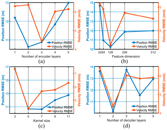
The RMSE comparison under different parameter settings is shown in Figure 6.

Figure 6. Comparison of position RMSE and velocity RMSE under different hyperparameter configurations. (a) Effect of encoder layers. (b) Effect of feature dimension. (c) Effect of convolution kernel size. (d) Effect of decoder layers.

The encoder consists of the dilated convolution branch and the multi-head self-attention branch in parallel. Both branches share the same number of layers, denoted as $N$. Increasing depth enhances the extraction of higher-order motion features, while excessive depth introduces overfitting. Except for $N$, the other parameters are fixed with $D=128$, $K=3$, and $N_d=2$. Figure 6a illustrates how the tracking errors vary with $N$. It can be observed that both metrics decrease when $N$ increases from 1 to 2. At $N=3$, the velocity RMSE further drops while the position RMSE slightly rebounds. Further increasing $N$ causes both errors to increase. The feature dimension $D$ controls the capacity of the high-dimensional mapping space. A larger value enriches feature representation, whereas an excessively large value causes parameter redundancy. Figure 6b presents the tracking errors at different feature dimensions $D$. Both position and velocity RMSEs continuously decrease as $D$ increases from 32 to 128. When $D$ further increases to 256, both errors rise significantly. The kernel size $K$ defines the local temporal receptive field of the dilated causal convolution. A small kernel may miss complete maneuver patterns. A large kernel introduces irrelevant noise. Figure 6c presents the tracking errors at different kernel sizes $K$. The tracking performance reaches its optimum at $K=3$. The number of decoder layers $N_d$ determines how effectively the model captures long-term temporal dependencies. A small value restricts the integration of contextual information, while a large value increases the risk of overfitting. Figure 6d depicts the influence of $N_d$ on the tracking errors. At $N_d=1$, both errors are relatively large due to insufficient temporal feature extraction. When $N_d$ increases to 2, both metrics reach their minimum. When $N_d$ further increases to 3 or more, both errors rise again.

In summary, the optimal parameter configuration is $N=3$, $D=128$, $K=3$, and $N_d=2$. All subsequent experiments adopt this configuration.

4.3. Ablation Study

This section evaluates the contribution of each core module through ablation experiments. All experiments run under the same hyperparameter configuration, and key modules are removed or replaced sequentially. The configurations of the ablation models are listed in Table 3, and the corresponding results are reported in Table 4.

Table 3. Component design of ablation models.

Model	Local Feature Extraction	Global Feature Extraction	Feature Fusion	Decoder
M1	Conv1D	J-MHSA	J-AF	J-BiLSTM
M2	DRC	MHSA	J-AF	J-BiLSTM
M3	DRC	J-MHSA	AF	J-BiLSTM
M4	DRC	J-MHSA	J-AF	BiLSTM
Ours	DRC	J-MHSA	J-AF	J-BiLSTM

Table 4. Ablation experiment results.

Model	The Position RMSE (m)	The Velocity RMSE (m/s)
M1	$13.99\pm 8.47$	$6.87\pm 21.79$
M2	$12.52\pm 7.70$	$6.41\pm 17.12$
M3	$13.77\pm 7.50$	$6.05\pm 14.16$
M4	$12.84\pm 8.18$	$7.14\pm 19.60$
Ours	$11.62\pm 6.97$	$4.43\pm 8.90$

Table 4 shows the position and velocity RMSEs of all ablation models. The complete JAF-MTT achieves the best results on both metrics, confirming the contribution of each module.

M1 substitutes the dilated residual convolution with standard 1D convolution. Its position RMSE rises by 20.4%, and the velocity RMSE climbs by 55.1%. The velocity RMSE standard deviation reaches 21.79, reflecting severe estimation fluctuation and poor stability under high-maneuver motion. M2 drops the jerk modulation in the global feature extraction branch by employing standard MHSA. The resulting position RMSE increases by 7.7%, and the velocity RMSE rises by 44.7%. Without jerk-driven guidance, errors accumulate progressively during consecutive maneuver switches. M3 replaces the jerk-aware adaptive fusion with ordinary adaptive fusion. The position RMSE goes up by 18.50%, and the velocity RMSE grows by 36.57%. This conventional adaptive fusion scheme fails to dynamically allocate feature weights according to maneuver intensity, leading to imbalanced feature representation. Its position RMSE standard deviation reaches 8.50, the highest among all variants. M4 replaces the jerk-modulated bidirectional LSTM (J-BiLSTM) with a standard BiLSTM. Its velocity RMSE surges by 61.2%, the most severe degradation among all variants. Without the explicit guidance of the jerk signal, the standard BiLSTM relies solely on hidden states for gating. Consequently, the forget and input gates cannot adjust their response amplitudes in time when the target suddenly switches from smooth motion to high maneuver, causing a lag in decoder state updates.

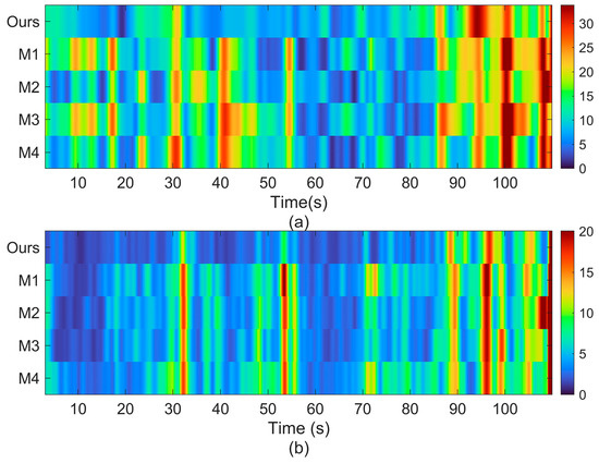
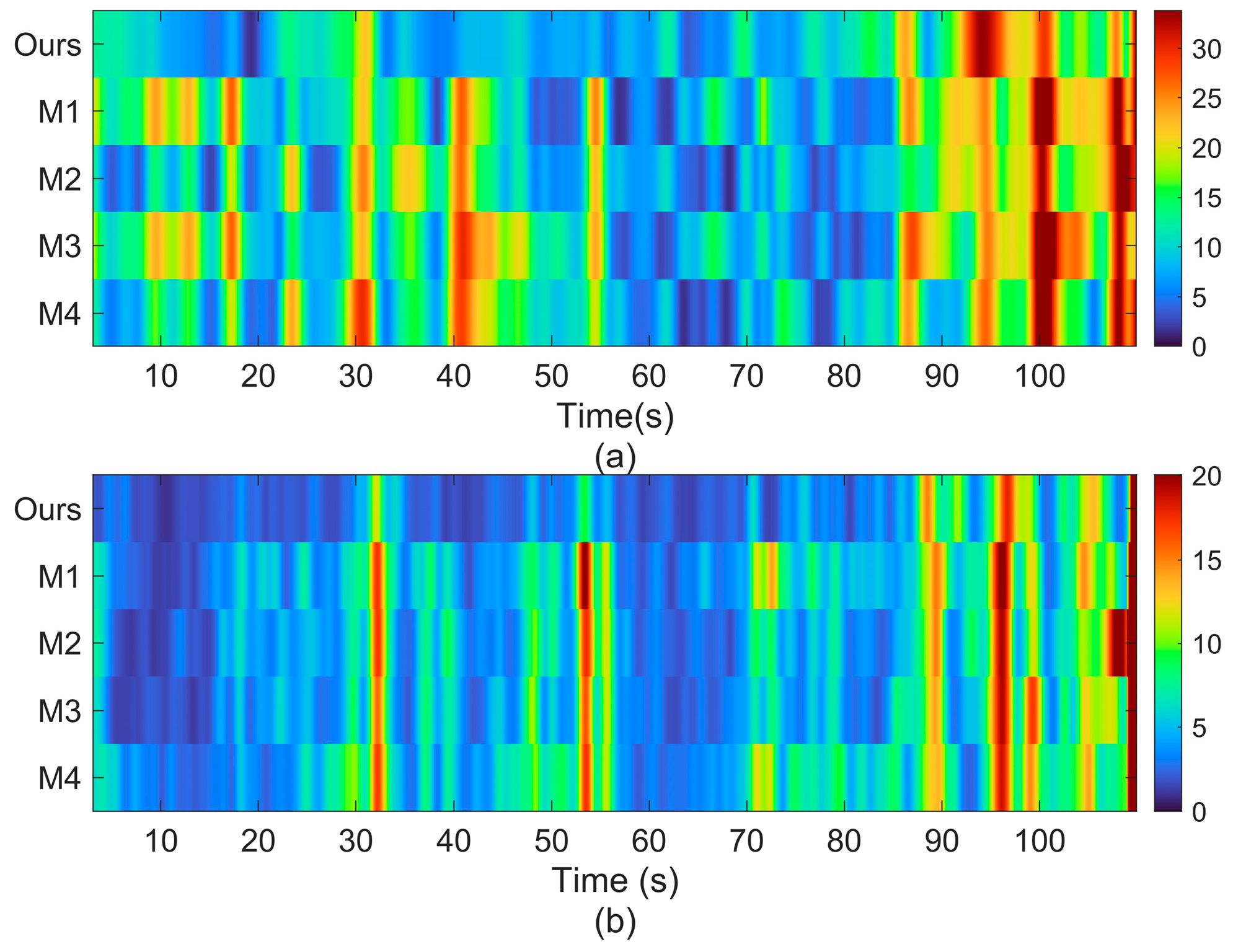
The temporal error heatmaps of all ablation models on trajectory H2 are shown in Figure 7. The horizontal axis represents the time step, the vertical axis lists different models, and the color depth indicates the error magnitude, with cool tones corresponding to low errors and warm tones to high errors.

Figure 7. Temporal error heatmaps of different ablation models on the full trajectory H2. (a) Position RMSE. (b) Velocity RMSE.

The JAF-MTT row consistently exhibits the lightest cool tones, indicating the lowest errors across the entire time domain. In particular, no abrupt color changes appear at maneuver-switching points, demonstrating its fast response to instantaneous maneuvers. In contrast, M1 shows distinct warm patches near switching points due to the delayed response of standard convolution. M2 develops persistent warm regions in later maneuver stages, reflecting error accumulation caused by the absence of global modeling. M3 displays generally warm tones across the whole time domain, reflecting the weak robustness of fixed fusion weights after removing jerk only from the fusion module. The velocity heatmap of M4 reveals multiple bright spots, confirming that removing jerk modulation degrades velocity estimation stability.

In summary, each core module in the JAF-MTT framework makes an irreplaceable contribution to the final tracking performance.

4.4. Comparative Experiments

This section compares the proposed JAF-MTT with five baseline algorithms, including IMM [8], VSIMM [18], DeepMTT [22], GRU-MTT [31], TrMTT [24] and KalmanNet [32]. All algorithms run under the same hardware environment and software framework for fair comparison.

For traditional model-driven methods, the IMM algorithm combines one constant velocity (CV) model and twelve constant turn (CT) models. Its turn rate is uniformly quantized within $[-{16}^{°}/s,{16}^{°}/s]$. The diagonal elements of the Markov transition matrix are set to 0.97, and initial model probabilities follow uniform distribution. The standard deviation of process noise is 10⁻³ rad/s, and the acceleration noise is 10 $\mathrm{m}/{\mathrm{s}}^2$ The VSIMM algorithm employs a model group switching (MGS) strategy to update active model sets dynamically with a switching threshold of 0.1. It shares the same model library and filtering parameters with IMM.

For deep learning-based methods, all models adopt unified training settings. The Adam optimizer is used with a batch size of 256 and an initial learning rate of 0.001. The learning rate is halved every 40 training epochs. The gradient clipping threshold is set to 1. The maximum training epoch is set to 120. Early stopping is applied to avoid overfitting. The input representation and parameter scale of each deep learning tracking model are summarized in Table 5.

Table 5. Implementation details of deep learning tracking models.

Algorithm	Input Representation	Trainable Parameters
KalmanNet	Innovation and state prediction vector	0.1 M
DeepMTT	64-step output sequence of CV-UKF	1.5 M
GRU-MTT	32-step trajectory observation sequence	0.8 M
TrMTT	32-step smoothed position velocity and acceleration features	1.8 M
JAF-MTT	32-frame-normalized observation sequence with jerk aware fusion	1 M

To comprehensively evaluate tracking performance, we design three categories of test trajectories covering different motion characteristics:

• Four trajectories with $\omega \in [-{15}^{°}/\mathrm{s},{15}^{°}/\mathrm{s}]$, following standard CV/CT motions within the training range for a basic tracking test.
• Two trajectories with intense turns, exceeding the training distribution for a generalization test.
• Two trajectories with coordinated acceleration and mixed motions, beyond conventional CV/CT rules for a general feature tests.

The detailed parameter settings of all test trajectories are summarized in Table 6.

Table 6. Parameter settings for test trajectories.

Trajectories	$\mathrm{initial} \mathrm{state} [\mathsf{x},\mathsf{y},{\mathsf{v}}_{\mathsf{x}},{\mathsf{v}}_{\mathsf{y}}]$	$1\mathrm{st} \mathrm{segment}$	$2\mathrm{nd} \mathrm{segment}$	$3\mathrm{rd} \mathrm{segment}$	$4\mathrm{th} \mathrm{segment}$	$5\mathrm{th} \mathrm{segment}$	$6\mathrm{th} \mathrm{segment}$
$\mathrm{H}1$	$\left[0,0,280,45\right]$	$20 \mathrm{s},0^{°}/\mathrm{s}$	$25 \mathrm{s},6^{°}/\mathrm{s}$	$20 \mathrm{s},-3^{°}/\mathrm{s}$	$20 \mathrm{s},-{12}^{°}/\mathrm{s}$	$35 \mathrm{s},3^{°}/\mathrm{s}$	$-$
$\mathrm{H}2$	$\left[10000,10000,200,180\right]$	$20 \mathrm{s},0^{°}/\mathrm{s}$	$20 \mathrm{s},6^{°}/\mathrm{s}$	$20 \mathrm{s},9^{°}/\mathrm{s}$	$20 \mathrm{s},{12}^{°}/\mathrm{s}$	$20 \mathrm{s},0^{°}/\mathrm{s}$	$-$
$\mathrm{H}3$	$[6000,20000,233,-59]$	$30 \mathrm{s},{11}^{°}/\mathrm{s}$	$40 \mathrm{s},-3^{°}/\mathrm{s}$	$30 \mathrm{s},-9^{°}/\mathrm{s}$	$-$	$-$	$-$
$\mathrm{H}4$	$[-20000,0,300,0]$	$15 \mathrm{s},8^{°}/\mathrm{s}$	$10 \mathrm{s},-{12}^{°}/\mathrm{s}$	$20 \mathrm{s},6^{°}/\mathrm{s}$	$12 \mathrm{s},-{10}^{°}/\mathrm{s}$	$15 \mathrm{s},8^{°}/\mathrm{s}$	$-$
$\mathrm{S}1$	$[22000,-6000,200,90]$	$10 \mathrm{s},0^{°}/\mathrm{s}$	$30 \mathrm{s},8^{°}/\mathrm{s}$	$25 \mathrm{s},{12}^{°}/\mathrm{s}$	$25 \mathrm{s},{16}^{°}/\mathrm{s}$	$20 \mathrm{s},{20}^{°}/\mathrm{s}$	$-$
$\mathrm{S}2$	$[15000,-20000,280,170]$	$30 \mathrm{s},9^{°}/\mathrm{s}$	$20 \mathrm{s},0^{°}/\mathrm{s}$	$8 \mathrm{s},{25}^{°}/\mathrm{s}$	$10 \mathrm{s},-{20}^{°}/\mathrm{s}$	$12 \mathrm{s},{15}^{°}/\mathrm{s}$	$16 \mathrm{s},-{25}^{°}/\mathrm{s}$
$\mathrm{A}1$	$[-15000,-5000,320,0]$	$15 \mathrm{s},0^{°}/\mathrm{s}$	$12 \mathrm{s},{15}^{°}/\mathrm{s}$	$10 \mathrm{s},-{18}^{°}/\mathrm{s}$	$15 \mathrm{s},0^{°}/\mathrm{s}$	$12 \mathrm{s},{12}^{°}/\mathrm{s}$	$15 \mathrm{s},0^{°}/\mathrm{s}$
$\mathrm{A}2$	$\left[4000,16000,260,10\right]$	$20 \mathrm{s},5^{°}/\mathrm{s}$	$35 \mathrm{s},-{10}^{°}/\mathrm{s}$	$20 \mathrm{s},-5^{°}/\mathrm{s}$	$10 \mathrm{s},0^{°}/\mathrm{s}$	$25 \mathrm{s},{25}^{°}/\mathrm{s}$	$-$

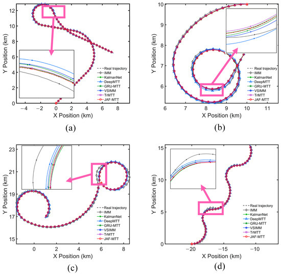
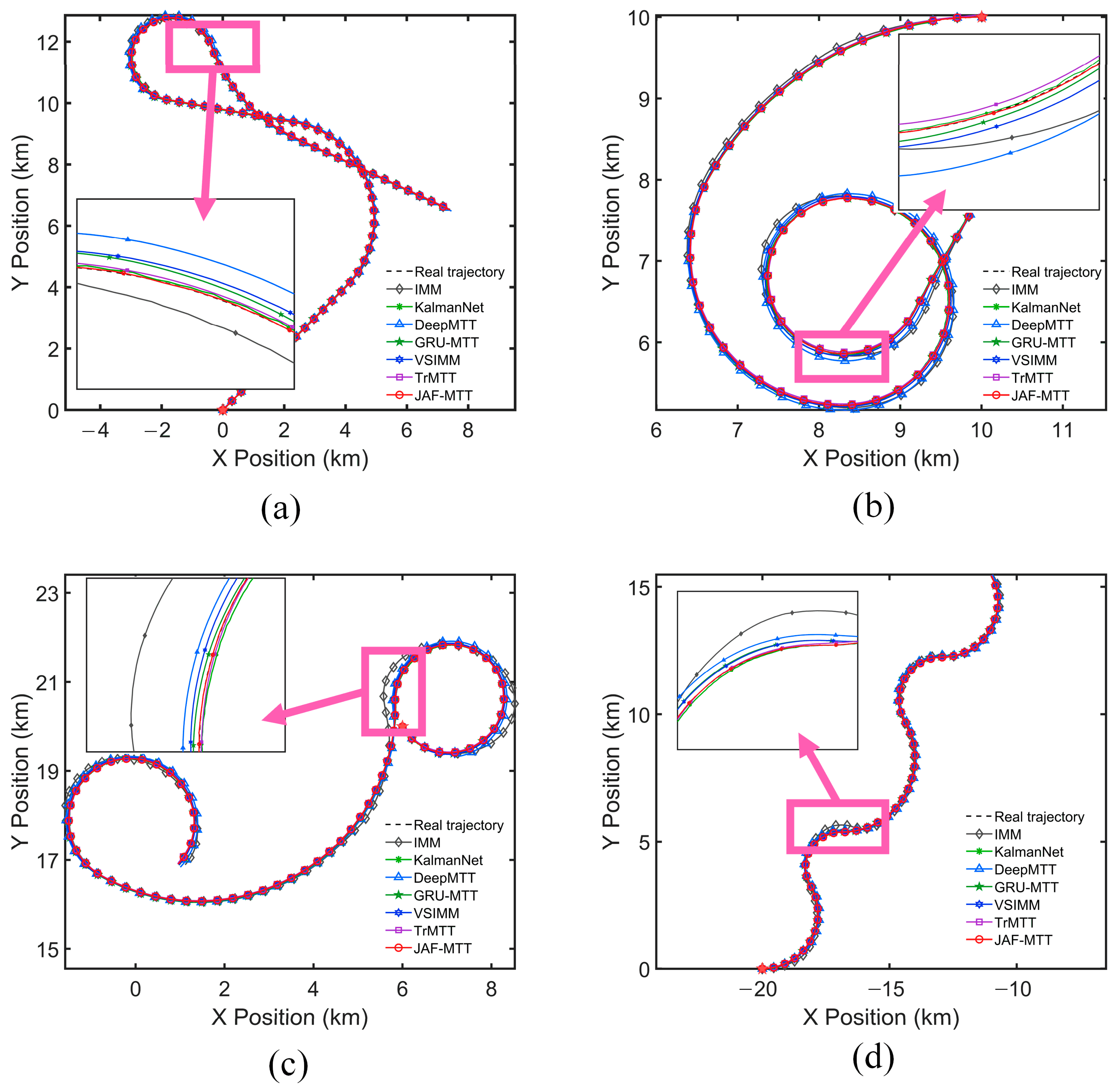
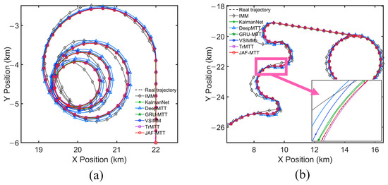
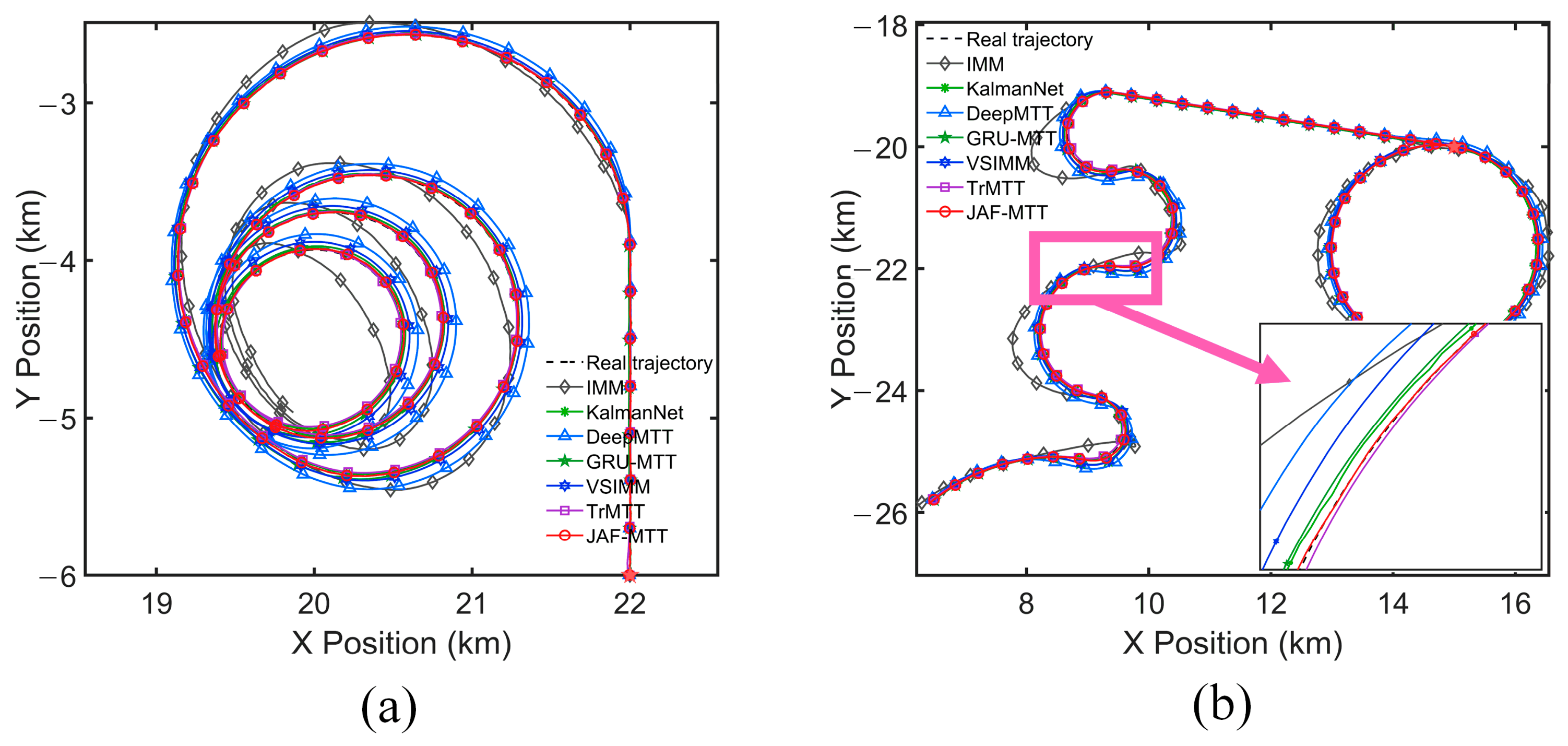
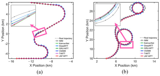
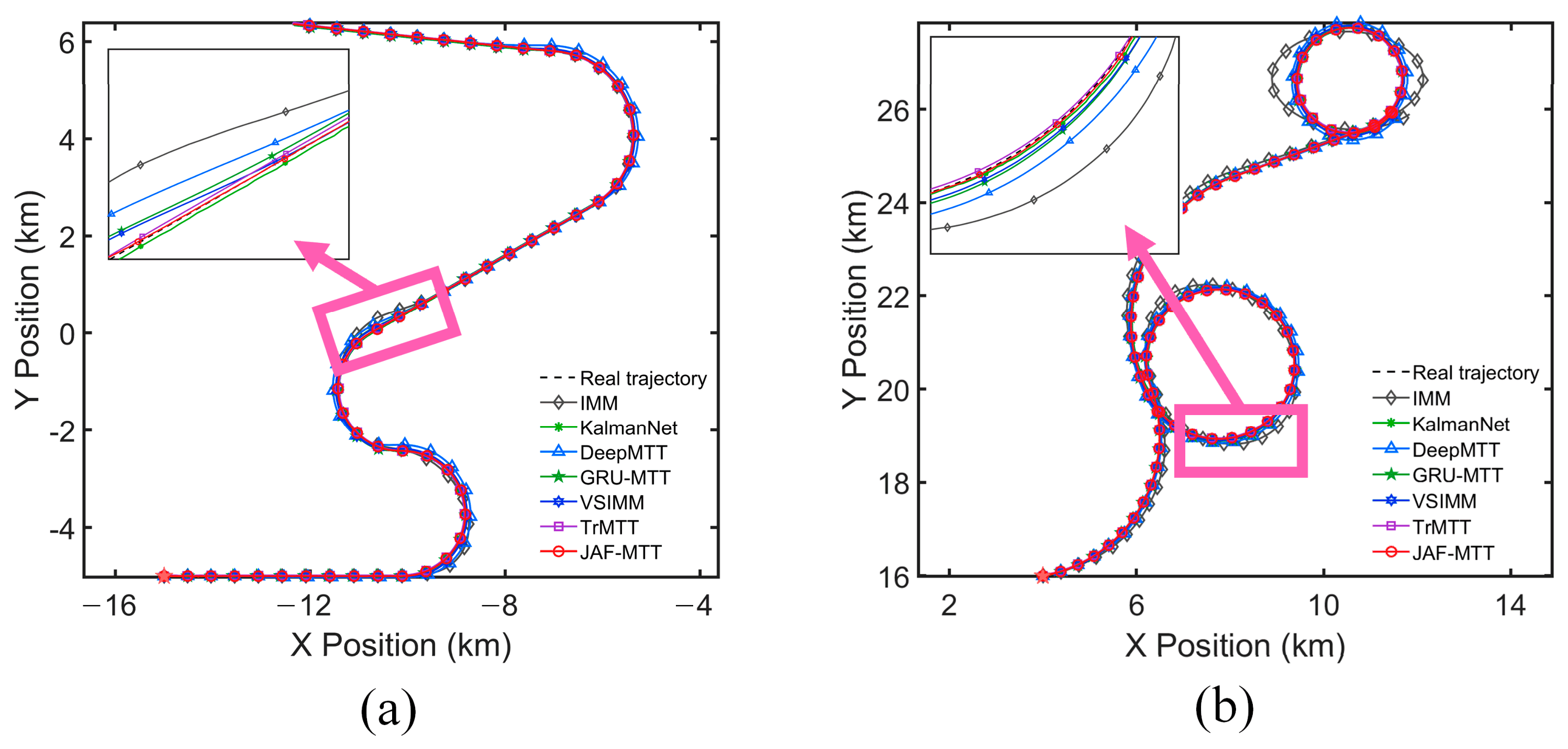
The statistical results of position RMSE and velocity RMSE for all algorithms on the eight maneuvering trajectories are summarized in Table 7. JAF-MTT consistently achieves the lowest RMSEs, and its advantage grows more pronounced as the maneuver intensity increases. The tracking performance comparison is illustrated in Figure 8, Figure 9 and Figure 10.

Table 7. Detailed tracking RMSE comparison of test trajectories.

Trajectories		$\mathsf{H}1$	$\mathsf{H}2$	$\mathsf{H}3$	$\mathsf{H}4$	$\mathsf{S}1$	$\mathsf{S}2$	$\mathsf{A}1$	$\mathsf{A}2$
$\begin{array}{l}\mathrm{Methods}\\ \left(\begin{array}{l}\mathrm{Mean}/\\ \mathrm{Deviation}\end{array}\right)\end{array}$		$\begin{array}{c}1\mathrm{st} \mathrm{segment}\\ 2\mathrm{nd} \mathrm{segment}\\ 3\mathrm{rd} \mathrm{segment}\\ 4\mathrm{th} \mathrm{segment} \\ 5\mathrm{th} \mathrm{segment}\\ 6\mathrm{th} \mathrm{segment}\end{array}$	$\begin{array}{c}1\mathrm{st} \mathrm{segment}\\ 2\mathrm{nd} \mathrm{segment}\\ 3\mathrm{rd} \mathrm{segment}\\ 4\mathrm{th} \mathrm{segment} \\ 5\mathrm{th} \mathrm{segment}\\ 6\mathrm{th} \mathrm{segment}\end{array}$	$\begin{array}{c}1\mathrm{st} \mathrm{segment}\\ 2\mathrm{nd} \mathrm{segment}\\ 3\mathrm{rd} \mathrm{segment}\\ 4\mathrm{th} \mathrm{segment} \\ 5\mathrm{th} \mathrm{segment}\\ 6\mathrm{th} \mathrm{segment}\end{array}$	$\begin{array}{c}1\mathrm{st} \mathrm{segment}\\ 2\mathrm{nd} \mathrm{segment}\\ 3\mathrm{rd} \mathrm{segment}\\ 4\mathrm{th} \mathrm{segment} \\ 5\mathrm{th} \mathrm{segment}\\ 6\mathrm{th} \mathrm{segment}\end{array}$	$\begin{array}{c}1\mathrm{st} \mathrm{segment}\\ 2\mathrm{nd} \mathrm{segment}\\ 3\mathrm{rd} \mathrm{segment}\\ 4\mathrm{th} \mathrm{segment} \\ 5\mathrm{th} \mathrm{segment}\\ 6\mathrm{th} \mathrm{segment}\end{array}$	$\begin{array}{c}1\mathrm{st} \mathrm{segment}\\ 2\mathrm{nd} \mathrm{segment}\\ 3\mathrm{rd} \mathrm{segment}\\ 4\mathrm{th} \mathrm{segment} \\ 5\mathrm{th} \mathrm{segment}\\ 6\mathrm{th} \mathrm{segment}\end{array}$	$\begin{array}{c}1\mathrm{st} \mathrm{segment}\\ 2\mathrm{nd} \mathrm{segment}\\ 3\mathrm{rd} \mathrm{segment}\\ 4\mathrm{th} \mathrm{segment} \\ 5\mathrm{th} \mathrm{segment}\\ 6\mathrm{th} \mathrm{segment}\end{array}$	$\begin{array}{c}1\mathrm{st} \mathrm{segment}\\ 2\mathrm{nd} \mathrm{segment}\\ 3\mathrm{rd} \mathrm{segment}\\ 4\mathrm{th} \mathrm{segment} \\ 5\mathrm{th} \mathrm{segment}\\ 6\mathrm{th} \mathrm{segment}\end{array}$
$\mathrm{IMM}$	$\begin{array}{l}\mathrm{Pos}\\ \left(\mathrm{m}\right)\end{array}$	$\begin{array}{c}2.23/5.75\\ 29.98/15.38\\ 6.64/8.61\\ 96.5/70.57\\ 9.37/5.34\\ -\end{array}$	$\begin{array}{c}25.83/11.34\\ 27.73/14.65\\ 58.16/28.54\\ 75.96/34.59\\ 24.88/33.22\\ -\end{array}$	$\begin{array}{c}168.09/98.75\\ 73.45/37.02\\ 107.30/71.83\\ -\\ -\\ -\end{array}$	$\begin{array}{c}122.76/47.15\\ 174.39/86.74\\ 67.45/28.75\\ 59.25/29.71\\ 302.75/165.91\\ -\end{array}$	$\begin{array}{c}114.00/75.79\\ 39.75/26.25\\ 257.81/167.53\\ 207.88/193.43\\ 241.67/137.29\\ 252.06/210.20\end{array}$	$\begin{array}{c}12.49/5.96\\ 127.29/73.65\\ 99.39/95.67\\ 45.03/76.82\\ 42.79/22.73\\ 4.07/2.67\end{array}$	$\begin{array}{c}28.50/24.25\\ 17.72/15.21\\ 29.95/23.65\\ 34.71/25.36\\ 41.42/27.45\\ 34.21/24.45\end{array}$	$\begin{array}{c}96.24/45.85\\ 192.76/94.81\\ 120.50/55.58\\ 94.19/54.33\\ 338.80/96.35\\ -\end{array}$
	$\begin{array}{l}\mathrm{Velo}\\ (\mathrm{m}/\mathrm{s})\end{array}$	$\begin{array}{c}12.50/25.14\\ 15.65/14.15\\ 7.56/8.03\\ 18.96/11.78\\ 6.06/4.75\\ -\end{array}$	$\begin{array}{c}36.53/28.88\\ 20.14/19.19\\ 27.03/22.71\\ 28.98/22.28\\ 46.26/36.24\\ -\end{array}$	$\begin{array}{c}46.54/36.18\\ 23.99/22.31\\ 13.52/10.82\\ -\\ -\\ -\end{array}$	$\begin{array}{c}32.95/28.17\\ 44.53/34.61\\ 40.52/33.16\\ 56.51/42.34\\ 88.55/73.78\\ -\end{array}$	$\begin{array}{c}146.39/143.50\\ 87.25/90.63\\ 131.94/119.76\\ 76.09/74.51\\ 114.13/100.31\\ 77.57/62.76\end{array}$	$\begin{array}{c}21.37/17.78\\ 30.20/21.44\\ 30.96/24.60\\ 5.35/5.26\\ 7.35/6.16\\ 8.64/6.81\end{array}$	$\begin{array}{c}28.50/24.25\\ 17.72/15.21\\ 29.95/23.65\\ 34.71/25.36\\ 41.42/27.45\\ 19.85/16.34\end{array}$	$\begin{array}{c}17.61/6.69\\ 819.54/12.98\\ 110.07/8.78\\ 713.39/7.67\\ 170.97/49.84\\ -\end{array}$
	$\mathrm{All}$	$20.66/36.46$	$37.15/31.32$	$69.81/73.87$	$108.53/112.73$	$136.37/140.24$	$33.23/54.61$	$87.27/63.36$	$136.37/62.24$
$\mathrm{VSIMM}$	$\begin{array}{l}\mathrm{Pos}\\ \left(\mathrm{m}\right)\end{array}$	$\begin{array}{c}21.78/8.78\\ 16.50/5.34\\ 26.35/3.07\\ 44.73/8.33\\ 24.25/7.37\\ -\end{array}$	$\begin{array}{c}12.09/4.18\\ 20.63/8.29\\ 16.58/5.83\\ 23.25/10.96\\ 17.27/2.12\\ -\end{array}$	$\begin{array}{c}20.80/10.73\\ 22.90/7.37\\ 29.93/9.62\\ -\\ -\\ -\end{array}$	$\begin{array}{c}15.96/5.88\\ 36.81/11.84\\ 30.22/9.19\\ 29.99/9.24\\ 53.39/14.61\\ -\end{array}$	$\begin{array}{c}25.10/12.01\\ 26.54/5.49\\ 56.10/19.77\\ 54.25/13.61\\ 39.89/14.60\\ 26.32/24.70\end{array}$	$\begin{array}{c}32.32/10.53\\ 39.38/7.24\\ 62.47/13.82\\ 40.92/9.14\\ 31.88/6.76\\ 27.07/3.16\end{array}$	$\begin{array}{c}13.47/6.79\\ 16.12/7.63\\ 22.05/8.63\\ 29.56/11.05\\ 36.74/8.50\\ 22.65/9.56\end{array}$	$\begin{array}{c}16.34/5.89\\ 35.55/5.25\\ 23.74/3.06\\ 16.38/1.92\\ 62.90/9.91\\ -\end{array}$
	$\begin{array}{l}\mathrm{Velo}\\ (\mathrm{m}/\mathrm{s})\end{array}$	$\begin{array}{c}3.62/6.28\\ 5.14/4.04\\ 7.88/5.92\\ 9.90/6.43\\ 6.37/4.63\\ -\end{array}$	$\begin{array}{c}23.11/51.64\\ 4.39/3.42\\ 7.10/5.42\\ 6.94/5.54\\ 8.30/6.16\\ -\end{array}$	$\begin{array}{c}25.43/56.87\\ 10.06/8.33\\ 9.51/8.21\\ -\\ -\\ -\end{array}$	$\begin{array}{c}28.34/61.16\\ 13.33/11.35\\ 10.55/8.69\\ 15.74/12.70\\ 23.57/17.85\\ -\end{array}$	$\begin{array}{c}27.50/65.47\\ 13.08/9.28\\ 19.33/12.35\\ 19.29/12.97\\ 16.81/15.04\\ 20.90/17.14\end{array}$	$\begin{array}{c}21.61/45.02\\ 8.31/7.01\\ 13.56/9.43\\ 2.40/3.26\\ 5.93/4.57\\ 3.94/2.98\end{array}$	$\begin{array}{c}59.59/109.51\\ 12.21/10.25\\ 12.81/11.50\\ 13.67/10.85\\ 14.25/10.90\\ 14.69/9.45\end{array}$	$\begin{array}{c}27.50/65.47\\ 13.08/9.28\\ 19.33/12.35\\ 19.29/12.97\\ 16.81/15.04\\ -\end{array}$
	$\mathrm{All}$	$16.62/13.53$	$13.97/18.61$	$19.44/24.63$	$26.53/25.27$	$23.48/22.95$		$20.69/27.66$	$27.92/33.05$
$\mathrm{KalmanNet}$	$\begin{array}{l}\mathrm{Pos}\\ \left(\mathrm{m}\right)\end{array}$	$\begin{array}{c}19.75/5.68\\ 13.42/2.64\\ 28.35/7.06\\ 20.82/8.37\\ 22.96/5.59\\ -\end{array}$	$\begin{array}{c}10.14/2.75\\ 18.02/5.83\\ 18.10/7.41\\ 24.57/8.25\\ 19.25/3.42\\ -\end{array}$	$\begin{array}{c}22.75/9.35\\ 20.85/8.42\\ 19.78/8.75\\ -\\ -\\ -\end{array}$	$\begin{array}{c}12.14/4.25\\ 35.52/11.15\\ 36.58/8.75\\ 30.49/7.25\\ 29.27/16.24\\ -\end{array}$	$\begin{array}{c}17.68/10.68\\ 24.47/4.75\\ 42.38/18.24\\ 53.17/13.35\\ 19.68/12.75\\ 20.24/20.68\end{array}$	$\begin{array}{c}28.75/9.68\\ 34.68/6.78\\ 54.57/10.57\\ 38.45/8.24\\ 32.55/7.35\\ 25.41/4.25\end{array}$	$\begin{array}{c}9.48/5.78\\ 12.12/7.68\\ 19.55/8.89\\ 25.56/12.35\\ 29.75/9.42\\ -\end{array}$	$\begin{array}{c}12.81/9.28\\ 21.52/13.80\\ 16.10/11.42\\ 3.56/1.22\\ 19.93/12.98\\ -\end{array}$
	$\begin{array}{l}\mathrm{Velo}\\ (\mathrm{m}/\mathrm{s})\end{array}$	$\begin{array}{c}2.45/6.86\\ 4.26/5.25\\ 8.78/3.14\\ 4.45/4.53\\ 5.14/2.55\\ -\end{array}$	$\begin{array}{c}18.25/23.75\\ 4.75/3.35\\ 6.23/4.74\\ 8.75/4.53\\ 7.24/5.75\\ -\end{array}$	$\begin{array}{c}18.45/34.45\\ 12.01/7.52\\ 10.42/9.75\\ -\\ -\\ -\end{array}$	$\begin{array}{c}19.04/20.53\\ 9.05/14.75\\ 12.38/5.58\\ 14.25/12.65\\ 15.36/14.68\\ -\end{array}$	$\begin{array}{c}20.47/35.28\\ 16.68/7.75\\ 14.37/22.69\\ 18.38/10.42\\ 14.58/12.14\\ 21.25/7.38\end{array}$	$\begin{array}{c}16.42/23.68\\ 9.75/10.35\\ 14.66/11.63\\ 3.75/4.37\\ 4.83/3.43\\ 2.44/3.35\end{array}$	$\begin{array}{c}19.72/29.51\\ 12.21/9.35\\ 11.88/9.59\\ 12.69/9.65\\ 12.75/10.54\\ -\end{array}$	$\begin{array}{c}16.11/11.85\\ 15.11/11.71\\ 15.58/12.58\\ 12.16/8.84\\ 13.80/11.48\\ -\end{array}$
	$\mathrm{All}$	$15.63/10.75$	$14.75/6.24$	$16.75/20.12$	$19.20/18.14$	$23.41/24.35$	$26.25/23.75$	$19.63/18.86$	$19.92/13.05$
$\mathrm{DeepMTT}$	$\begin{array}{l}\mathrm{Pos}\\ \left(\mathrm{m}\right)\end{array}$	$\begin{array}{c}19.18/12.09\\ 49.25/6.74\\ 13.78/11.16\\ 76.88/23.53\\ 67.54/8.73\\ -\end{array}$	$\begin{array}{c}19.51/8.22\\ 53.78/12.79\\ 64.23/4.84\\ 72.31/14.67\\ 30.95/12.67\\ -\end{array}$	$\begin{array}{c}64.40/27.25\\ 39.70/13.72\\ 64.58/18.66\\ -\\ -\\ -\end{array}$	$\begin{array}{c}36.68/16.90\\ 76.28/18.00\\ 43.82/6.49\\ 34.74/6.11\\ 152.62/33.99\\ -\end{array}$	$\begin{array}{c}71.99/26.53\\ 17.28/21.08\\ 123.92/52.97\\ 130.82/41.34\\ 95.85/33.19\\ 57.22/62.1\end{array}$	$\begin{array}{c}30.39/16.90\\ 121.01/27.59\\ 114.62/42.19\\ 52.53/25.43\\ 100.75/20.66\\ 35.39/26.93\end{array}$	$\begin{array}{c}23.53/11.72\\ 49.69/9.91\\ 74.91/10.52\\ 91.20/14.10\\ 107.76/9.64\\ 86.45/10.46\end{array}$	$\begin{array}{c}35.09/22.07\\ 79.12/17.80\\ 45.64/5.68\\ 32.30/2.46\\ 128.11/26.53\\ -\end{array}$
	$\begin{array}{l}\mathrm{Velo}\\ (\mathrm{m}/\mathrm{s})\end{array}$	$\begin{array}{c}6.55/19.75\\ 5.61/4.46\\ 7.24/5.81\\ 18.39/8.86\\ 7.64/6.02\\ -\end{array}$	$\begin{array}{c}38.48/62.60\\ 5.98/4.26\\ 9.75/7.32\\ 15.45/7.77\\ 9.35/7.53\\ -\end{array}$	$\begin{array}{c}46.70/91.14\\ 10.87/8.28\\ 13.42/10.55\\ -\\ -\\ -\end{array}$	$\begin{array}{c}49.17/80.11\\ 16.76/13.26\\ 12.04/10.30\\ 18.73/14.34\\ 52.26/26.22\\ -\end{array}$	$\begin{array}{c}45.32/90.75\\ 13.35/9.93\\ 38.69/22.07\\ 35.58/19.55\\ 29.68/17.74\\ 25.04/17.45\end{array}$	$\begin{array}{c}35.52/63.20\\ 22.65/12.19\\ 25.64/14.37\\ 8.97/14.36\\ 16.07/9.11\\ 5.68/4.87\end{array}$	$\begin{array}{c}111.80/151.97\\ 13.38/10.23\\ 17.38/12.85\\ 26.14/14.63\\ 33.59/15.38\\ 20.34/13.52\end{array}$	$\begin{array}{c}13.27/32.29\\ 12.54/4.78\\ 5.22/3.88\\ 2.20/1.73\\ 30.68/11.65\\ -\end{array}$
	$\mathrm{All}$	$28.49/28.08$	$31.98/31.65$	$38.48/44.29$	$53.40/50.96$	$54.84/59.85$	$44.66/46.98$	$51.42/48.42$	$49.84/39.85$
$\mathrm{GRU}‐\mathrm{MTT}$	$\begin{array}{l}\mathrm{Pos}\\ \left(\mathrm{m}\right)\end{array}$	$\begin{array}{c}11.12/10.24\\ 22.36/4.75\\ 12.75/10.15\\ 16.36/18.25\\ 10.75/7.35\\ -\end{array}$	$\begin{array}{c}10.25/4.24\\ 18.54/8.86\\ 14.54/5.42\\ 16.32/8.02\\ 18.76/2.01\\ -\end{array}$	$\begin{array}{c}16.35/9.42\\ 14.24/10.89\\ 10.87/9.36\\ -\\ -\\ -\end{array}$	$\begin{array}{c}13.25/5.35\\ 26.11/10.25\\ 22.63/8.04\\ 20.45/9.36\\ 52.36/12.75\\ -\end{array}$	$\begin{array}{c}21.24/10.85\\ 26.55/5.78\\ 46.24/17.57\\ 24.35/13.25\\ 59.75/11.10\\ 16.32/20.42\end{array}$	$\begin{array}{c}10.86/12.41\\ 19.98/7.27\\ 24.69/10.68\\ 29.75/9.17\\ 11.36/6.69\\ 20.42/3.75\end{array}$	$\begin{array}{c}23.63/12.22\\ 26.23/2.81\\ 24.22/11.52\\ 35.75/12.18\\ 27.56/10.84\\ 27.22/20.16\end{array}$	$\begin{array}{c}12.84/6.26\\ 38.58/11.57\\ 30.60/7.23\\ 35.44/1.96\\ 15.55/11.62\\ -\end{array}$
	$\begin{array}{l}\mathrm{Velo}\\ (\mathrm{m}/\mathrm{s})\end{array}$	$\begin{array}{c}4.42/17.36\\ 6.85/7.25\\ 7.45/1.18\\ 15.68/4.14\\ 6.64/5.68\\ -\end{array}$	$\begin{array}{c}18.14/16.25\\ 4.57/3.77\\ 7.42/5.36\\ 6.55/5.24\\ 8.80/6.17\\ -\end{array}$	$\begin{array}{c}20.45/12.75\\ 8.76/8.36\\ 9.38/8.42\\ -\\ -\\ -\end{array}$	$\begin{array}{c}20.42/18.68\\ 10.25/11.33\\ 10.74/8.53\\ 18.14/10.47\\ 8.42/12.25\\ -\end{array}$	$\begin{array}{c}28.57/35.14\\ 13.75/9.55\\ 29.34/15.47\\ 19.36/14.36\\ 16.57/12.55\\ 30.36/12.42\end{array}$	$\begin{array}{c}18.04/12.36\\ 8.25/7.22\\ 12.99/8.46\\ 3.55/3.27\\ 4.36/4.86\\ 3.94/2.42\end{array}$	$\begin{array}{c}11.36/19.93\\ 2.30/1.75\\ 14.58/9.25\\ 15.14/8.63\\ 25.23/14.35\\ 28.35/15.34\end{array}$	$\begin{array}{c}6.98/19.57\\ 5.09/2.66\\ 2.71/2.13\\ 1.64/1.16\\ 8.81/3.72\\ -\end{array}$
	$\mathrm{All}$	$18.35/19.75$	$15.58/15.51$	$16.36/18.75$	$26.25/25.88$	$30.75/35.36$	$19.57/18.36$	$24.52/16.89$	$29.84/19.85$
$\mathrm{TrMTT}$	$\begin{array}{l}\mathrm{Pos}\\ \left(\mathrm{m}\right)\end{array}$	$\begin{array}{c}1.52/0.84\\ 10.60/5.12\\ 14.90/3.17\\ 14.95/7.92\\ 8.49/3.67\\ -\end{array}$	$\begin{array}{c}7.18/4.29\\ 5.79/3.22\\ 9.15/3.14\\ 8.30/3.38\\ 6.35/3.22\\ -\end{array}$	$\begin{array}{c}17.04/7.31\\ 10.87/6.10\\ 15.08/7.65\\ -\\ -\\ -\end{array}$	$\begin{array}{c}9.55/5.08\\ 18.72/8.88\\ 17.59/7.06\\ 16.29/7.96\\ 42.20/19.65\\ -\end{array}$	$\begin{array}{c}21.76/9.50\\ 16.41/5.60\\ 43.22/19.24\\ 30.35/13.72\\ 33.02/11.32\\ 21.32/12.19\end{array}$	$\begin{array}{c}7.82/5.35\\ 20.93/4.75\\ 20.53/6.62\\ 4.69/4.07\\ 12.21/5.07\\ 7.35/3.32\end{array}$	$\begin{array}{c}12.09/7.79\\ 9.49/4.83\\ 17.37/7.72\\ 19.19/8.83\\ 23.54/7.77\\ 18.42/3.24\end{array}$	$\begin{array}{c}11.76/6.50\\ 6.41/8.60\\ 33.22/5.24\\ 20.35/3.72\\ 23.02/9.32\\ -\end{array}$
	$\begin{array}{l}\mathrm{Velo}\\ (\mathrm{m}/\mathrm{s})\end{array}$	$\begin{array}{c}7.89/5.63\\ 14.29/10.92\\ 14.42/11.07\\ 13.77/11.10\\ 10.67/9.64\\ -\end{array}$	$\begin{array}{c}32.75/50.09\\ 17.03/13.83\\ 21.65/16.12\\ 17.31/13.96\\ 24.85/19.44\\ -\end{array}$	$\begin{array}{c}33.86/56.31\\ 18.27/13.92\\ 13.30/12.04\\ -\\ -\\ -\end{array}$	$\begin{array}{c}37.57/59.71\\ 24.74/18.65\\ 20.90/18.41\\ 27.18/21.62\\ 32.42/26.54\\ -\end{array}$	$\begin{array}{c}42.45/66.17\\ 24.48/18.59\\ 24.73/21.40\\ 28.51/19.77\\ 28.10/20.41\\ 23.08/17.22\end{array}$	$\begin{array}{c}28.05/42.25\\ 15.19/12.20\\ 16.62/13.81\\ 5.05/3.81\\ 8.81/6.82\\ 12.94/10.62\end{array}$	$\begin{array}{c}70.25/107.14\\ 23.22/19.96\\ 24.20/20.16\\ 24.24/21.11\\ 23.86/19.33\\ 12.24/16.37\end{array}$	$\begin{array}{c}4.45/10.17\\ 4.48/2.59\\ 2.73/2.40\\ 1.51/1.77\\ 6.10/1.41\\ -\end{array}$
	$\mathrm{All}$	$11.15/9.41$	$15.04/20.84$	$17.72/24.72$	$25.16/25.84$	$29.06/32.69$	$12.95/16.41$	$22.17/29.41$	$19.06/9.69$
	$\mathrm{CI}$	$[9.31,12.99]$	$[10.96,19.12]$	$[12.87,22.57]$	$[20.10,30.22]$	$[22.65,35.47]$	$[9.73,16.17]$	$[16.41,27.93]$	$[17.16,20.96]$
$\mathrm{JAF}‐\mathrm{MTT}$	$\begin{array}{l}\mathrm{Pos}\\ \left(\mathrm{m}\right)\end{array}$	$\begin{array}{c}13.59/2.07\\ 5.54/3.22\\ 5.30/0.80\\ 9.33/2.70\\ 12.74/1.66\\ -\end{array}$	$\begin{array}{c}3.66/1.84\\ 12.18/2.37\\ 7.29/3.95\\ 12.09/4.60\\ 7.59/3.29\\ -\end{array}$	$\begin{array}{c}11.11/4.37\\ 5.30/2.46\\ 9.40/3.19\\ -\\ -\\ -\end{array}$	$\begin{array}{c}7.27/2.82\\ 8.36/5.44\\ 5.10/1.92\\ 10.25/3.05\\ 20.72/6.58\\ -\end{array}$	$\begin{array}{c}12.94/5.46\\ 3.69/1.78\\ 25.73/5.43\\ 13.89/5.24\\ 18.47/6.62\\ 6.42/3.66\end{array}$	$\begin{array}{c}10.09/3.64\\ 9.10/4.75\\ 13.00/2.87\\ 11.43/1.76\\ 10.12/5.27\\ 6.86/3.74\end{array}$	$\begin{array}{c}6.79/4.26\\ 7.93/6.12\\ 9.86/3.59\\ 12.10/4.96\\ 16.78/6.76\\ 8.63/2.24\end{array}$	$\begin{array}{c}6.94/5.46\\ 3.69/1.78\\ 12.73/2.43\\ 10.89/2.24\\ 6.47/1.62\\ -\end{array}$
	$\begin{array}{l}\mathrm{Velo}\\ (\mathrm{m}/\mathrm{s})\end{array}$	$\begin{array}{c}3.72/14.43\\ 2.20/1.62\\ 2.21/1.65\\ 2.30/1.91\\ 1.80/1.39\\ -\end{array}$	$\begin{array}{c}3.59/3.91\\ 1.62/1.23\\ 2.10/1.83\\ 2.59/1.67\\ 3.24/4.82\\ -\end{array}$	$\begin{array}{c}4.25/7.82\\ 2.70/2.43\\ 2.90/3.77\\ -\\ -\\ -\end{array}$	$\begin{array}{c}2.94/5.38\\ 3.58/2.91\\ 3.03/2.26\\ 5.36/3.71\\ 10.27/26.62\\ -\end{array}$	$\begin{array}{c}4.72/15.77\\ 3.49/2.81\\ 10.27/5.68\\ 6.48/3.92\\ 5.00/3.17\\ 4.66/4.40\end{array}$	$\begin{array}{c}5.18/18.56\\ 3.88/2.56\\ 3.83/2.33\\ 0.82/0.81\\ 2.26/1.68\\ 3.32/6.70\end{array}$	$\begin{array}{c}9.14/25.24\\ 2.94/2.29\\ 3.16/2.46\\ 3.84/2.63\\ 7.35/24.09\\ 4.53/1.24\end{array}$	$\begin{array}{c}2.72/5.77\\ 1.49/2.81\\ 6.27/5.68\\ 4.48/3.92\\ 5.00/3.17\\ -\end{array}$
	$\mathrm{All}$	$6.09/7.22$	$5.59/4.95$	$5.75/5.27$	$7.80/11.15$	$9.07/9.94$	$6.57/7.70$	$7.69/10.73$	$7.07/4.94$
	$\mathrm{CI}$	$[4.67,7.51]$	$[4.62,6.56]$	$[4.72,6.78]$	$[5.61,9.99]$	$[7.12,11.02]$	$[5.06,8.08]$	$[5.59,9.79]$	$[6.10,8.04]$

Figure 8. Comparison of tracking trajectories of different algorithms in high-maneuver scenarios. (a) Trajectory H1. (b) Trajectory H2. (c) Trajectory H3. (d) Trajectory H4.

Figure 9. Comparison of tracking results of different algorithms in ultra-maneuver scenarios. (a) Trajectory S1. (b) Trajectory S2.

Figure 10. Comparison of tracking results of different algorithms in mixed acceleration–turn scenarios. (a) Trajectory A1. (b) Trajectory A2.

The model-driven methods accumulate larger errors in high-maneuver scenarios. IMM uses a fixed model set. Its error increases significantly during continuous large-angle turns. On trajectories H3 and H4, its position RMSE is much higher than that of other algorithms, indicating severe model mismatch. VSIMM improves the tracking accuracy by introducing a dynamic model set adjustment mechanism. On most high-maneuver trajectories, its error is about one-third to one-half of that of IMM. However, in ultra-maneuver scenarios, VSIMM still produces considerably higher errors than the data-driven methods. This suggests that predefined physical models have limited capacity to represent unknown maneuver patterns.

All data-driven approaches achieve better overall performance yet still have inherent drawbacks under intense maneuvers. DeepMTT works reliably for low-dynamic motion, but prominent tracking lag occurs during high maneuvers, leading to elevated position and velocity RMSE. KalmanNet obtains moderate tracking accuracy and exhibits evident oscillations at turning segments. GRU-MTT generates smoother trajectories than DeepMTT, though cumulative lag still exists when the target moves rapidly. Benefiting from the Transformer architecture, TrMTT achieves further accuracy gains. On high-maneuver trajectories, its position error is approximately half that of DeepMTT. Nevertheless, severe velocity fluctuations appear at sharp ultra-maneuver turns, and its local errors are far larger than those of JAF-MTT.

In contrast, JAF-MTT maintains the lowest position and velocity RMSEs on all test trajectories. Even in ultra-maneuver scenarios beyond the training distribution, its error growth is considerably smaller than that of the competing methods. In velocity estimation, JAF-MTT achieves a velocity RMSE below 6 m/s in most trajectory segments. This demonstrates the effectiveness of the jerk modulation mechanism in capturing abrupt velocity changes. Moreover, the non-overlapping 95% confidence intervals between JAF-MTT and TrMTT across all eight trajectories demonstrate that the improvement in tracking accuracy is statistically significant, rather than a product of random simulation fluctuations.

Figure 8 shows the tracking trajectories of all algorithms compared with the true trajectory. IMM and DeepMTT exhibit the largest deviations. During the consecutive maneuver switches in Figure 8b, both algorithms lag notably behind the true trajectory. KalmanNet performs moderately, with visible oscillations at some turn points but less drift than IMM. GRU-MTT tracks more smoothly than DeepMTT, yet still shows a mild lag in fast-changing segments. VSIMM and TrMTT achieve relatively good overall alignment, but the zoomed-in areas still reveal slight fluctuations at maneuver switches. In contrast, JAF-MTT stays tightly aligned with the true trajectory across all segments, with smooth transitions at every switch.

Figure 9 shows the tracking trajectories of all algorithms in ultra-maneuver scenarios. As the maneuver intensity exceeds the training distribution, the estimated trajectories of the competing algorithms deviate more noticeably from the true trajectory. This is especially pronounced in Figure 9a. IMM loses its tracking ability after the second turn, and its estimated curve deviates significantly from the true trajectory. DeepMTT consistently lags behind the true motion, and the lag increases as the number of turns grows. KalmanNet oscillates and occasionally diverges. GRU-MTT suffers from cumulative lag and gradually drifts away from the true path. TrMTT exhibits more pronounced jumps at maneuver-switching points. In contrast, JAF-MTT still closely follows the true trajectory, with only minor fluctuations.

Figure 10 further tests the algorithms on complex motion patterns including coordinated acceleration and combined acceleration–turn movements, which are beyond conventional CV and CT models. Other methods suffer from obvious lag and phase shift, whereas JAF-MTT matches the true trajectory best and responds stably to both acceleration and turning motions.

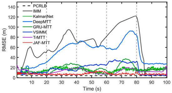
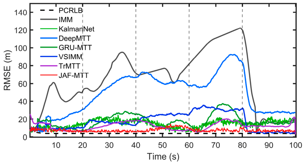
To further evaluate the practical tracking performance against the theoretical optimum, the Posterior Cramer-Rao Lower Bound (PCRLB) is adopted as the theoretical lower bound for position RMSE [15]. The results on trajectory H2 are plotted in Figure 11, where the PCRLB acts as a reliable benchmark for tracking accuracy evaluation.

Figure 11. RMSE comparison between all algorithms and the PCRLB on trajectory H2.

As shown in Figure 11, the RMSE curves of all algorithms stay above the PCRLB. Among all competing algorithms, the proposed JAF-MTT maintains position RMSE consistently closest to this theoretical lower bound, which verifies its excellent tracking accuracy.

Apart from tracking accuracy, computational efficiency is also critical for practical engineering. Accordingly, we further evaluate the computational performance of all algorithms.

As illustrated in Table 8, the proposed JAF-MTT achieves favorable computational efficiency and runs faster than most deep learning baselines, which makes it well suited for real-time maneuvering target tracking.

Table 8. Comparison of computation time.

Algorithm	Computation Time (s)
IMM	0.2648
VSIMM	0.4435
KalmanNet	0.8435
DeepMTT	1.5399
GRU-MTT	2.1406
TrMTT	3.0769
JAF-MTT	1.0348

4.5. Noise Robustness Analysis

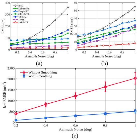
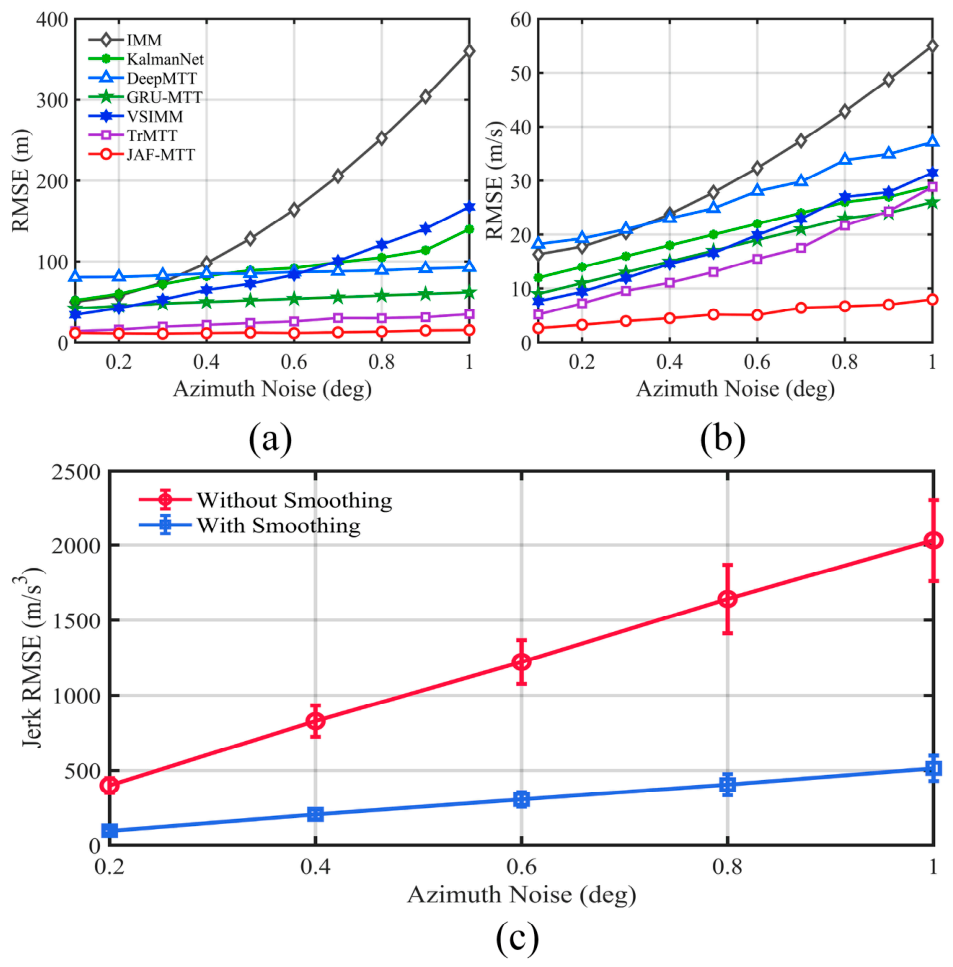
This section assesses the impact of measurement noise on tracking accuracy. Trajectory H4 from Section 4.3 is selected as the test case. The azimuth error introduces position bias that increases with the target range during the conversion from polar measurements to Cartesian coordinates. For distant targets, this effect is much larger than that of the range error [31,32]. The range noise standard deviation is fixed at ${\sigma }_{\rho }=10 \mathrm{m}$, and the azimuth noise standard deviation ${\sigma }_{\theta }$ is gradually increased from ${0.2}^{°}$ to $1^{°}$. The RMSE curves of position and velocity for competing algorithms are plotted in Figure 12a,b. As noisy UCM-converted coordinates introduce notable noise amplification after multi-order differentiation for jerk derivation, Figure 12c quantifies the smoothing’s noise-suppression effect under identical test settings.

Figure 12. Comparison of tracking performance under different azimuth noise levels. (a) Position RMSE. (b) Velocity RMSE. (c) Jerk RMSE comparison with and without smoothing.

With the increase in azimuth noise, the tracking accuracy of various algorithms decreases at distinctly different rates. The IMM algorithm suffers the most severe performance degradation. Its position RMSE rises from about 50 m at low noise to over 350 m at high noise, and its velocity RMSE increases similarly. The RMSEs of DeepMTT, VSIMM, KalmanNet, GRU-MTT and TrMTT grow more slowly. At ${\sigma }_{\theta }=1^{°}$, DeepMTT has a position RMSE of about 100 m and a velocity RMSE of about 40 m/s. KalmanNet and GRU-MTT exhibit similar growth trends with medium error magnitudes. VSIMM and TrMTT have slightly lower errors than DeepMTT, but they still remain at high levels. In contrast, JAF-MTT achieves the lowest tracking error at all noise levels. At ${\sigma }_{\theta }=1^{°}$, its position RMSE is only about 20 m, and its velocity RMSE is about 10 m/s. Moreover, its RMSE grows the slowest with increasing noise.

From Figure 12c, jerk estimation errors grow monotonically with rising azimuth noise for both calculation approaches, and the vertical error bars further reflect the statistical fluctuation of results over repeated simulations. The adopted smoothing reduces the average jerk RMSE by around 78% across all noise levels. Such evident error reduction confirms that smoothing effectively suppresses differentiation-induced noise and stabilizes jerk features for subsequent feature fusion.

The noise resilience of JAF-MTT stems from its encoder structure and the jerk modulation mechanism. The encoder captures temporal patterns across multiple receptive field scales, preserving effective feature extraction even under strong noise. Meanwhile, the jerk modulation mechanism adjusts the fusion weights according to maneuver intensity. It suppresses noise in smooth periods and captures state changes in high-maneuver periods. These results indicate that JAF-MTT has stronger robustness against measurement noise.

5. Conclusions

This paper proposes a JAF-MTT algorithm for high-maneuver scenarios. We adopt jerk as the indicator of maneuver intensity. A parallel structure consisting of convolution and multi-head self-attention is constructed to extract local and global trajectory features. These features are then adaptively fused based on maneuver intensity. Finally, we design a jerk-modulated bidirectional LSTM that decodes the fused features to obtain the target state estimate. Simulation results demonstrate that the proposed algorithm outperforms IMM, VSIMM, DeepMTT, and TrMTT in both high-maneuver and ultra-maneuver scenarios. Under high-maneuver conditions, the RMSE of JAF-MTT reaches 5.59 m. In comparison, the model-driven algorithms yield RMSEs of 37.15 m and 13.97 m, while the data-driven algorithms achieve RMSEs of 31.98 m and 15.04 m. JAF-MTT also demonstrates excellent performance in ultra-maneuver scenarios. As measurement noise increases, the proposed algorithm maintains strong noise robustness, with its tracking error consistently remaining the lowest among all compared methods.

It is worth noticing that this study focuses on two-dimensional scenarios for method validation. Future work will extend JAF-MTT to three-dimensional tracking. We will examine methods for effectively capturing vertical motion features and investigate the implementation of multi-trajectory parallel tracking.

References

- Zhang, H.; Xie, J.; Ge, J.; Lu, W.; Liu, B. Strong tracking SCKF based on adaptive CS model for manoeuvring aircraft tracking. IET Radar Sonar Navig. 2018, 12, 742–749. [Google Scholar] [CrossRef] [Scilit]
- He, S.; Wu, P.; Li, X.; Bo, Y.; Yun, P. Adaptive Modified Unbiased Minimum-Variance Estimation for Highly Maneuvering Target Tracking with Model Mismatch. IEEE Trans. Instrum. Meas. 2023, 72, 8501216. [Google Scholar] [CrossRef] [Scilit]
- Zhao, Y.; Xie, Y.; Sun, Z.; Liu, W.; Wang, G.; Peng, S. Extended information filter for tracking high-speed target with maneuver. In Proceedings of the 2025 40th Youth Academic Annual Conference of Chinese Association of Automation (YAC), Zhengzhou, China, 17–19 May 2025; pp. 2044–2049. [Google Scholar] [CrossRef] [Scilit]
- Yang, M.; Meng, Z.J.; Jiang, R.Y.; Shi, H.B.; Chen, J.L. Tracking algorithm of powered phase of multi-stage ballistic missile based on improved adaptive “current” statistical model. J. Northwest. Polytech. Univ. 2025, 43, 843–852. [Google Scholar] [CrossRef] [Scilit]
- Zhao, X.; Lei, Z.; Yang, C.; Ma, Y. Robust and adaptive CKF-based adaptive parallel interacting multiple-model tracking algorithm for complex maneuvering targets. Discov. Appl. Sci. 2026, 8, 147. [Google Scholar] [CrossRef] [Scilit]
- Mehrotra, K.; Mahapatra, P.R. A jerk model for tracking highly maneuvering targets. IEEE Trans. Aerosp. Electron. Syst. 1997, 33, 1094–1104. [Google Scholar] [CrossRef] [Scilit]
- Mahapatra, P.R.; Mehrotra, K. Mixed coordinate tracking of generalized maneuvering targets using acceleration and jerk models. IEEE Trans. Aerosp. Electron. Syst. 2000, 36, 992–1000. [Google Scholar] [CrossRef] [Scilit]
- Blom, H.A.P.; Bar-Shalom, Y. The interacting multiple model algorithm for systems with Markovian switching coefficients. IEEE Trans. Autom. Control 1988, 33, 780–783. [Google Scholar] [CrossRef] [Scilit]
- Li, X.R.; Jilkov, V.P. Survey of maneuvering target tracking. Part I: Dynamic models. IEEE Trans. Aerosp. Electron. Syst. 2003, 39, 1333–1364. [Google Scholar] [CrossRef] [Scilit]
- Li, X.R.; Jilkov, V.P. Survey of maneuvering target tracking. Part V: Multiple-model methods. IEEE Trans. Aerosp. Electron. Syst. 2005, 41, 1255–1321. [Google Scholar] [CrossRef] [Scilit]
- Xu, L.; Li, X.; Duan, Z. Hybrid grid multiple-model estimation with application to maneuvering target tracking. IEEE Trans. Aerosp. Electron. Syst. 2016, 52, 122–136. [Google Scholar] [CrossRef] [Scilit]
- Li, X.R.; Jilkov, V.P. Multiple-model estimation with variable structure. IEEE Trans. Autom. Control 1996, 41, 478–493. [Google Scholar] [CrossRef] [Scilit]
- Li, X.R. Multiple-model estimation with variable structure. II. Model-set adaptation. IEEE Trans. Autom. Control 2000, 45, 2047–2060. [Google Scholar] [CrossRef] [Scilit]
- Li, X.R.; Zhi, X.R.; Zhang, Y.M. Multiple-model estimation with variable structure. III. Model-group switching algorithm. IEEE Trans. Aerosp. Electron. Syst. 1999, 35, 225–241. [Google Scholar] [CrossRef] [Scilit]
- Su, J.; Li, Y.; Ali, W. Underwater passive manoeuvring target tracking with isogradient sound speed profile. IET Radar Sonar Navig. 2022, 16, 1415–1433. [Google Scholar] [CrossRef] [Scilit]
- Li, X.R.; Jilkov, V.P.; Ru, J.F. Multiple-model estimation with variable structure- part VI: Expected-mode augmentation. IEEE Trans. Aerosp. Electron. Syst. 2005, 41, 853–867. [Google Scholar] [CrossRef] [Scilit]
- Tian, Y.; Fu, R.; Yan, H.; Xu, Z.; Peng, X. Gradient-Descent-Based STDM-VSIMM Filter for Maneuvering Target Tracking. IEEE Trans. Aerosp. Electron. Syst. 2025, 61, 16592–16605. [Google Scholar] [CrossRef] [Scilit]
- Huang, J.; Li, Z.; Liu, D.; Yang, Q.; Zhu, J. An adaptive state estimation for tracking hypersonic glide targets with model uncertainties. Aerosp. Sci. Technol. 2023, 136, 108235. [Google Scholar] [CrossRef] [Scilit]
- Zhou, H.; Zhang, C.; Peng, P.; Guo, Z. MambaMTT: A deep learning method based on mamba structure for maneuvering target tracking. Signal Process. 2026, 239, 110285. [Google Scholar] [CrossRef] [Scilit]
- Gao, C.; Yan, J.; Zhou, S.; Varshney, P.K.; Liu, H. Long short-term memory-based deep recurrent neural networks for target tracking. Inf. Sci. 2019, 502, 279–296. [Google Scholar] [CrossRef] [Scilit]
- Liu, J.; Wang, Z.; Xu, M. DeepMTT: A deep learning maneuvering target-tracking algorithm based on bidirectional LSTM network. Inf. Fusion 2020, 53, 289–304. [Google Scholar] [CrossRef] [Scilit]
- Yang, X.; Qiao, D. Attention-Based Bidirectional LSTM Network for Target Tracking. In Proceedings of the 2021 IEEE International Conference on Electronic Technology, Communication and Information (ICETCI), Changchun, China, 27–29 August 2021; pp. 151–156. [Google Scholar] [CrossRef] [Scilit]
- Zhang, Y.; Li, G.; Zhang, X.P.; He, Y. A deep learning model based on transformer structure for radar tracking of maneuvering targets. Inf. Fusion 2024, 103, 102120. [Google Scholar] [CrossRef] [Scilit]
- Shen, L.; Su, H.; Li, Z.; Jia, C.; Yang, R. Self-Attention-Based Transformer for Nonlinear Maneuvering Target Tracking. IEEE Trans. Geosci. Remote Sens. 2023, 61, 5109013. [Google Scholar] [CrossRef] [Scilit]
- Pinto, J.; Hess, G.; Ljungbergh, W.; Xia, Y.; Wymeersch, H.; Svensson, L. Deep Learning for Model-Based Multiobject Tracking. IEEE Trans. Aerosp. Electron. Syst. 2023, 59, 7363–7379. [Google Scholar] [CrossRef] [Scilit]
- Chen, H.; Bian, B.; Lian, F.; Zhang, W. Maneuvering extended target tracking method based on transformer network. Measurement 2025, 240, 115474. [Google Scholar] [CrossRef] [Scilit]
- Kim, J.; Kang, H.; Kang, P. Time-series anomaly detection with stacked Transformer representations and 1D convolutional network. Eng. Appl. Artif. Intell. 2023, 120, 105964. [Google Scholar] [CrossRef] [Scilit]
- Xia, L.; Zhang, S.; Hu, Y.; Zhang, R.; Li, S.; Sheng, W. A deep learning-based maneuvering target tracking with temporal convolutional networks. Signal Process 2023, 239, 110322. [Google Scholar] [CrossRef] [Scilit]
- Li, X.R.; Jilkov, V.P. Survey of Maneuvering Target Tracking. Part II: Motion Models of Ballistic and Space Targets. IEEE Trans. Aerosp. Electron. Syst. 2010, 46, 96–119. [Google Scholar] [CrossRef] [Scilit]
- Li, X.R.; Bar-Shalom, Y. Design of an interacting multiple model algorithm for air traffic control tracking. IEEE Trans. Contr. Syst. Technol. 1993, 1, 186–194. [Google Scholar] [CrossRef] [Scilit]
- Ma, C.; Yang, C.S.; Yang, F.; Zhuang, Y.Q.; Zhang, Z.W.; Jia, H.Z. Trajectory Factory: Tracklet cleaving and re-connection by deep Siamese Bi-GRU for multiple object tracking. In Proceedings of the 2018 IEEE International Conference on Multimedia and Expo (ICME), San Diego, CA, USA, 23–27 July 2018; IEEE: New York, NY, USA, 2018; Volume 1, pp. 1–6. [Google Scholar] [CrossRef] [Scilit]
- Mari, M.; Snidaro, L. Ensemble of KalmanNets with innovation-based attention for robust target tracking. Inf. Fusion 2026, 127, 103777. [Google Scholar] [CrossRef] [Scilit]
Disclaimer/Publisher’s Note: The statements, opinions and data contained in all publications are solely those of the individual author(s) and contributor(s) and not of MDPI and/or the editor(s). MDPI and/or the editor(s) disclaim responsibility for any injury to people or property resulting from any ideas, methods, instructions or products referred to in the content. |
© 2026 by the authors. Licensee MDPI, Basel, Switzerland. This article is an open access article distributed under the terms and conditions of the Creative Commons Attribution (CC BY) license.