A Joint Optimization Method for Radio Antenna Arrays Under Tri-Domain Errors and Atmospheric Effects Based on Improved Dueling DQN

Abstract

This paper presents a co-optimization framework for sparse concentric ring arrays based on an improved Dueling Deep Q-Network (DDQN) with a two-tier adaptive step-size strategy. The method aims at joint sidelobe suppression and structural optimization under non-ideal conditions. A tri-domain stochastic error model is introduced to characterize position, phase, and amplitude perturbations, and atmospheric-effect-aware evaluation is incorporated for high-frequency propagation scenarios. For a six-ring sparse array, radius-only optimization achieves a PSLL of $-24.4810$ dB, corresponding to an average improvement of $5.809$ dB over the initial array and an additional reduction compared with the baseline DDQN method. Extending the design to joint optimization of ring radii and element counts further reduces the PSLL to $-30.629$ dB, demonstrating the effectiveness of combined geometric and sparsity control. Monte Carlo simulations show that the optimized array maintains stable sidelobe performance under tri-domain stochastic perturbations, with an average PSLL of $-26.758$ dB. Further analysis using real meteorological data indicates that atmospheric effects introduce moderate variations in the normalized beam pattern, while the overall performance remains primarily influenced by stochastic perturbations under the considered modeling conditions. The proposed framework provides an effective and robust optimization approach for sparse concentric ring arrays in practical high-frequency scenarios.

1. Introduction

Sparse antenna arrays are widely used in a variety of high-frequency electromagnetic systems, including terrestrial millimeter-wave wireless communications, high-resolution sensing, and short-range high-frequency propagation systems, because they can provide high angular resolution and large effective apertures with reduced hardware complexity [1,2]. In contrast to astronomical radio observation scenarios, this work focuses on ground-based engineering applications. Among various sparse-array topologies, concentric ring arrays are particularly attractive due to their rotational symmetry, compact parameterization, and flexible beam-steering capability [3,4].

In this work, we focus on sparse array design for terrestrial high-frequency systems operating in the millimeter-wave (mmWave) band, particularly around 60 GHz. The target application is robust antenna-array design for terrestrial mmWave communication and sensing systems, rather than radio astronomy. This frequency range is representative of emerging 5G/6G communication and high-resolution sensing scenarios, where short wavelengths make array performance highly sensitive to both hardware imperfections (e.g., position deviations, phase jitter, and excitation fluctuations) and atmospheric propagation effects such as oxygen absorption and humidity-induced attenuation. In particular, the 60 GHz band is characterized by noticeable atmospheric oxygen absorption and strong sensitivity to array perturbations, making it a suitable test case for jointly analyzing hardware imperfections and propagation effects.

The performance of concentric ring arrays depends strongly on ring radii, the number of elements on each ring, and excitation settings. In this study, unless otherwise stated, equal-amplitude and in-phase excitation is assumed in the main experiments, so that the optimization focuses on geometric variables rather than excitation synthesis. A critical metric in array-pattern synthesis is the peak sidelobe level (PSLL), which must be carefully controlled. The synthesis problem is a constrained nonconvex optimization task with multiple local minima. This difficulty is further exacerbated by sparsity constraints, minimum inter-element spacing requirements, and structural regularity, especially under practical non-ideal conditions encountered in mmWave systems.

To address these challenges, this paper proposes a co-optimization framework for sparse concentric ring arrays based on an improved Dueling Deep Q-Network (DDQN) with a two-tier adaptive step-size strategy. The main contributions of this work are as follows:

• A collaborative design framework is established, enabling joint optimization of ring radii and per-ring element counts under a minimum inter-element spacing constraint.
• A tri-domain stochastic error model is introduced to characterize the combined effect of position, phase, and amplitude perturbations, allowing robustness evaluation within the optimization loop.
• A two-tier adaptive step-size strategy (global step-size adaptation module combined with ring-specific refinement) is proposed within the improved Dueling DQN framework. Its effectiveness is validated through ablation studies with 10 random seeds and prespecified permutation tests, demonstrating statistically significant improvement in PSLL.
• A dedicated post-optimization sensitivity analysis is conducted using real meteorological data, assessing the additional influence of atmospheric effects on the optimized beam pattern in a terrestrial mmWave propagation scenario.

It should be noted that the present work focuses on robustness against hardware-induced tri-domain stochastic perturbations and atmospheric propagation effects. External intentional interference, such as jamming signals, is not explicitly modeled in the current optimization framework. However, the proposed method can be extended by incorporating interference-aware performance metrics or jamming-related features into the optimization process, which will be considered in future work.

The remainder of this paper is organized as follows. Section 2 reviews related work. Section 3 presents the mathematical model of concentric ring arrays and formulates the optimization problem. Section 4 describes the improved Dueling DQN algorithm. Section 5 reports simulation results and performance comparisons. Section 6 provides a detailed discussion of the results. Finally, Section 7 concludes the paper and outlines future research directions.

2. Related Work

The design of sparse array layouts has been investigated through a variety of deterministic, stochastic, and learning-based approaches. Early methods focused on physically motivated strategies for sidelobe reduction. Kogan [5] proposed a deterministic strategy for reducing PSLL, while Boone [6,7] introduced a gas analogy model on the $uv$ plane. More recently, Girard et al. [8] applied modified simulated annealing to minimize the integrated sidelobe level. Although these methods provide valuable theoretical insights, their applicability to high-dimensional, mixed-variable problems with multiple constraints (such as sparsity and minimum spacing) remains limited.

To overcome these limitations, various heuristic and stochastic algorithms have been adopted, including combinations of Invasive Weed Optimization and Particle Swarm Optimization [4], 0–1 programming with differential evolution [9], non-uniform Fourier transforms [10], Bessel-function-based formulations [11]. For concentric ring arrays specifically, these methods can effectively suppress sidelobes but generally rely on iterative search strategies that are sensitive to initialization and prone to local minima. More importantly, most existing approaches address only a subset of the challenges—few methods jointly optimize sparsity, structural parameters, and robustness under stochastic perturbations within a unified framework.

With recent advances in deep reinforcement learning (DRL), data-driven strategies have emerged as promising alternatives for antenna-array optimization [12]. However, existing DRL-based works typically treat only partial aspects of the problem and lack integrated handling of tri-domain hardware errors and environmental effects.

In addition to conventional sparse-array synthesis, recent studies have explored geometry-aware and physically reconfigurable electromagnetic systems, such as movable antennas, movable intelligent surfaces (MISs), and mechanically or rotationally reconfigurable array architectures. These approaches introduce additional spatial degrees of freedom by dynamically adjusting the physical positions or configurations of radiating or reflecting elements, thereby enabling more flexible beam-pattern control. For example, movable intelligent surface (MIS) systems exploit controllable spatial displacement or configuration changes of intelligent surfaces to improve wireless communication performance through joint optimization of structural and electromagnetic parameters [13]. Similarly, movable antenna systems and mechanically reconfigurable arrays adjust element positions or orientations to adapt radiation patterns to dynamic environments.

Despite their effectiveness, these approaches differ fundamentally from the problem considered in this work. First, MISs and movable antenna systems typically rely on runtime physical reconfiguration, whereas the present study focuses on design-stage structural optimization of sparse concentric ring arrays through ring radii and element-count allocation. Second, existing geometry-reconfigurable systems are primarily evaluated using communication-oriented metrics, while this work targets robust peak sidelobe level (PSLL) suppression under tri-domain stochastic perturbations. Third, atmospheric effects are usually not explicitly incorporated into the optimization process in prior work, whereas this study provides a post-optimization sensitivity analysis to assess environmental impact. Therefore, the proposed method complements existing geometry-aware designs by providing a robust optimization framework for sparse array synthesis under practical non-ideal conditions.

To address the limitations of existing methods and focus on robust array optimization under non-ideal conditions, this paper adopts an improved Dueling DQN formulation integrated with a tri-domain perturbation model and a two-tier adaptive step-size mechanism.

3. The Optimization Model of Sparse Concentric Ring Array

3.1. Array Modeling Under Ideal Conditions

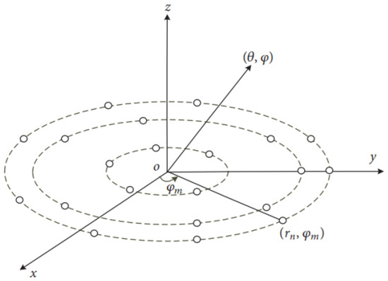
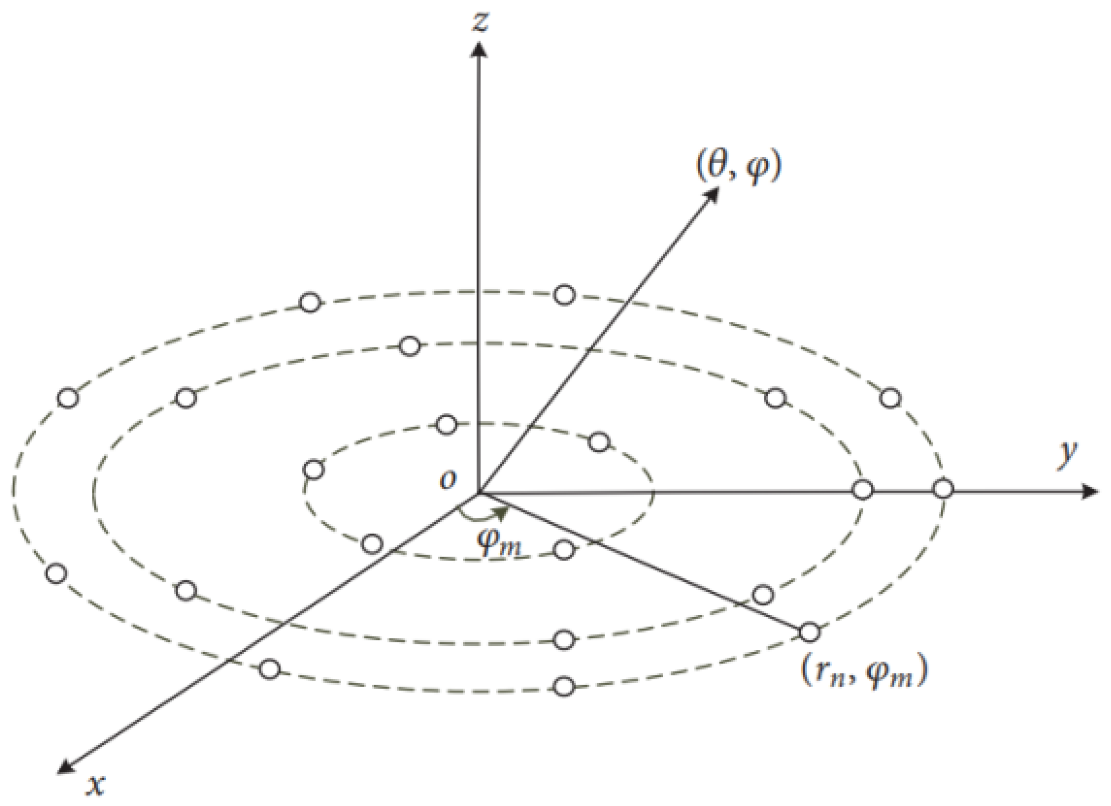
As shown in Figure 1, the planar array is constructed by first placing a central element at the origin. Multiple concentric rings with different radii are then generated around this center, with a number of elements uniformly distributed along each ring, resulting in a sparse concentric ring array configuration [3].

Figure 1. Schematic diagram of the concentric circle array model.

To avoid notational ambiguity, K is used throughout this paper to denote the number of concentric rings excluding the central element. The central element is indexed by $k=0$, with $r_0=0$ and $N_0=1$. For the k-th ring, $r_k$ denotes the ring radius and $N_k$ denotes the number of active elements on this ring.

For a ring-wise uniform angular distribution, the angular position of the m-th element on the k-th ring is defined as

$${\phi }_{k,m}={\displaystyle \frac{2\pi (m-1)}{N_k}},m=1,\dots ,N_k.$$

(1)

When the central element is fixed at the origin, the array factor of the thinned concentric ring array can be expressed as [3,4]

$$F(u,v)=1+{\displaystyle \sum _{k=1}^K}{\omega }_k{\displaystyle \sum _{m=1}^{N_k}}\exp \left[j{k}_0{r}_k\left(\cos {\phi }_{k,m}u+\sin {\phi }_{k,m}v\right)\right]$$

(2)

where $N_k$ represents the number of active elements on the k-th ring, K is the total number of concentric rings, $k_0=2\pi /\lambda$ is the wavenumber with $\lambda$ being the wavelength, ${\omega }_k$ denotes the excitation coefficient of the k-th ring, and $r_k$ is the radius of the k-th ring.

In this work, unless otherwise stated, equal-amplitude and in-phase excitation is assumed for all array elements in the main experiments. Specifically, the nominal excitation coefficients are set as ${\omega }_k=1$ for all rings in the ring-level formulation. In the element-level formulation, this corresponds to ${\alpha }_n=1$ and ${\psi }_n=0$ for all elements. Therefore, the optimization in this study focuses on geometric variables (ring radii and element counts), rather than excitation synthesis.

The spatial position of the m-th element on the k-th ring is defined in polar coordinates and converted into Cartesian coordinates as

$$(x_{k,m},y_{k,m})=\left(r_k\cos {\phi }_{k,m},r_k\sin {\phi }_{k,m}\right).$$

(3)

where $r_k$ and ${\phi }_{k,m}$ denote the radial distance and angular position of the m-th element on the k-th ring, respectively.

In the far-field region, the direction cosines corresponding to the observation angles are defined as

$$u=\sin \theta \cos \varphi ,v=\sin \theta \sin \varphi ,$$

(4)

where $\theta$ and $\varphi$ denote the elevation and azimuth angles, respectively.

The design of a sparse concentric ring array is subject to multiple constraints, including the maximum array aperture L, the minimum inter-element spacing $d_c$, and integer-valued ring-wise element counts. To clarify the difference between the two optimization settings used in this work, radius-only optimization and joint radius-and-count optimization are formulated separately.

In the first scenario, namely radius-only optimization, the ring-wise element counts are fixed as their initial values $N_k^{\left(0\right)}$. Therefore, the total number of active elements is fixed as

$$N_{\mathrm{act}}^{\left(0\right)}=1+{\displaystyle \sum _{k=1}^K}{N}_k^{\left(0\right)}.$$

(5)

Only the ring radii are optimized. The radius-only optimization problem is formulated as

$$\begin{array}{cc}\hfill \underset{\mathbf{r}}{\min }& \mathrm{PSLL}\left(\mathbf{r},{\mathbf{N}}^{\left(0\right)}\right)\hfill \\ \hfill \mathrm{subject}\mathrm{to}& 0<r_1<r_2<\cdots <r_K\le L,\hfill \\ \hfill & d_{\min }\left(\mathbf{r},{\mathbf{N}}^{\left(0\right)}\right)\ge d_c,\hfill \\ \hfill & N_{\mathrm{act}}=N_{\mathrm{act}}^{\left(0\right)},\hfill \end{array}$$

(6)

where $\mathbf{r}=[r_1,\dots ,r_K]$, ${\mathbf{N}}^{\left(0\right)}=[N_1^{\left(0\right)},\dots ,N_K^{\left(0\right)}]$, and $d_{\min }(·)$ denotes the minimum Euclidean distance among all active array elements.

In the second scenario, namely joint radius-and-count optimization, both the ring radii and the ring-wise element counts are optimized. The total number of active elements is no longer fixed, but is constrained within a prescribed range:

$$N_{\mathrm{act}}=1+{\displaystyle \sum _{k=1}^K}{N}_k,N_{\min }\le N_{\mathrm{act}}\le N_{\max }.$$

(7)

To explicitly account for hardware complexity, the joint optimization objective includes a sparsity-related penalty term:

$$\begin{array}{cc}\hfill \underset{\mathbf{r},\mathbf{N}}{\min }& \mathrm{PSLL}(\mathbf{r},\mathbf{N})+{\lambda }_N{\displaystyle \frac{N_{\mathrm{act}}}{N_{\max }}}\hfill \\ \hfill \mathrm{subject}\mathrm{to}& 0<r_1<r_2<\cdots <r_K\le L,\hfill \\ \hfill & N_{k,\min }\le N_k\le N_{k,\max },N_k\in \mathbb{Z},\hfill \\ \hfill & N_{\min }\le N_{\mathrm{act}}\le N_{\max },\hfill \\ \hfill & d_{\min }(\mathbf{r},\mathbf{N})\ge d_c.\hfill \end{array}$$

(8)

where ${\lambda }_N$ is a weighting coefficient used to balance sidelobe suppression and hardware complexity.

The PSLL is defined as the maximum sidelobe level beyond the first nulls of the main beam, which can be expressed as

$$\mathrm{PSLL}(\mathbf{r},\mathbf{N})=\underset{(\theta ,\varphi )\in {\Omega }_{\mathrm{sidelobe}}}{\max }\left\{20{\log }_{10}\left|{\displaystyle \frac{F(\theta ,\varphi )}{F_{\max }}}\right|\right\},$$

(9)

where $F_{\max }={\max }_{(\theta ,\varphi )}\left|F(\theta ,\varphi )\right|$, and ${\Omega }_{\mathrm{sidelobe}}$ denotes the angular region outside the main lobe, i.e., beyond the first nulls. The first nulls are determined numerically from the array factor.

In the numerical evaluation of PSLL, the radiation pattern is computed on a discrete angular grid. The first nulls of the main lobe are determined numerically as the nearest local minima on both sides of the main-beam peak. The sidelobe region ${\Omega }_{\mathrm{sidelobe}}$ is then defined as the angular domain outside these first-null points, and the PSLL is obtained as the maximum normalized pattern value within this region.

3.2. Array Modeling with Tri-Domain Errors and Atmospheric Effects

This study focuses on the 60 GHz frequency band in the millimeter-wave (mmWave) spectrum, which is widely used in terrestrial wireless communication and high-resolution sensing systems. The target application of this work is ground-based mmWave propagation scenarios, rather than astronomical radio observation.

The 60 GHz band is selected because it represents a typical high-frequency regime where two key characteristics coexist: (i) the short wavelength makes array performance highly sensitive to geometric configuration and hardware imperfections, and (ii) atmospheric oxygen absorption becomes non-negligible, introducing direction-dependent attenuation along the propagation path. Therefore, this frequency band provides a suitable test case for jointly analyzing array-structure optimization and propagation-related effects [14,15,16].

At this frequency, array performance is determined not only by the geometric configuration of the antennas but also by propagation-related effects, especially atmospheric absorption and phase fluctuations. In terrestrial line-of-sight propagation scenarios, oxygen absorption, water vapor, and temperature-dependent refractive-index variations may introduce additional attenuation and phase perturbations along the propagation path.

In practical arrays, the radiation performance is further affected by hardware- and environment-induced uncertainties, including excitation amplitude errors, excitation phase errors, and element position deviations caused by manufacturing tolerances, installation offsets, thermal drift, and other non-ideal factors. These effects may degrade the array factor, increase sidelobe levels, reduce gain, and weaken robustness. Therefore, they should be incorporated into the array modeling and optimization process.

3.2.1. Tri-Domain Random Error Model

This paper considers stochastic errors in the phase, amplitude, and position domains to model non-ideal array behavior [17,18].

First, phase-domain errors arise because, under ideal conditions, the excitation phase of each element is assumed to be exact. In practice, however, phase jitter in the feed network, oscillator instability, and other hardware imperfections introduce deviations from the nominal phase. These phase errors are modeled as independent Gaussian random variables:

$${ϵ}_{\psi ,n}\sim \mathcal{N}(0,{\sigma }_{\psi }^2),$$

(10)

with probability density function

$$f_{\psi }\left({ϵ}_{\psi ,n}\right)={\displaystyle \frac{1}{{\sigma }_{\psi }\sqrt{2\pi }}}\exp \left(-{\displaystyle \frac{{ϵ}_{\psi ,n}^2}{2{\sigma }_{\psi }^2}}\right).$$

(11)

Accordingly, the noisy excitation phase of the n-th element is written as

$${\psi }_{n,\mathrm{noise}}={\psi }_n+{ϵ}_{\psi ,n},$$

(12)

where ${\psi }_n$ denotes the nominal excitation phase of the n-th element.

To provide a unified control of stochastic perturbations, a normalized noise level parameter is introduced, denoted as $NL$. It is related to the phase-noise standard deviation by

$${\sigma }_{\psi }={\displaystyle \frac{NL}{20}},$$

(13)

where $NL$ is a user-defined parameter controlling the intensity of stochastic perturbations.

Second, amplitude-domain errors mainly arise from amplifier gain fluctuations, feedline loss variations, and other hardware imperfections. In this work, the amplitude error is modeled in the logarithmic domain by a Gaussian random variable, which leads to a log-normal perturbation in linear amplitude:

$${ϵ}_{\alpha ,n}\sim \mathcal{N}(0,{\sigma }_{\alpha }^2),$$

(14)

$${\alpha }_{n,\mathrm{noise}}={\alpha }_n{10}^{{ϵ}_{\alpha ,n}/20},$$

(15)

where ${\alpha }_n$ is the nominal excitation amplitude of the n-th element. Using the same noise level parameter, the standard deviation is given by

$${\sigma }_{\alpha }={\displaystyle \frac{NL}{20}}.$$

(16)

Third, position-domain errors describe the deviation between the actual installed position of an element and its nominal design position. Although the nominal array geometry is defined in polar coordinates, the installation offset is represented here in Cartesian coordinates on the array plane for convenience:

$$\delta {\mathbf{r}}_n=\left[\begin{array}{c}\delta x_n\\ \delta y_n\end{array}\right]\sim \mathcal{N}\left(\left[\begin{array}{c}0\\ 0\end{array}\right],\Sigma \right),$$

(17)

where

$$\Sigma =\left[\begin{array}{cc}{\sigma }_x^2& \rho {\sigma }_x{\sigma }_y\\ \rho {\sigma }_x{\sigma }_y& {\sigma }_y^2\end{array}\right],$$

(18)

and $\rho$ denotes the correlation coefficient between the two coordinate directions. The actual position vector is then

$${\mathbf{r}}_n^{\mathrm{act}}={\mathbf{r}}_n+\delta {\mathbf{r}}_n.$$

(19)

Finally, the array factor including the tri-domain errors is expressed as

$$A{F}_{\mathrm{noise}}(\theta ,\varphi )={\displaystyle \sum _{n=1}^N}{\alpha }_{n,\mathrm{noise}}\exp \left\{j\left[{\psi }_{n,\mathrm{noise}}+{\displaystyle \frac{2\pi }{\lambda }}{\mathbf{r}}_n^{\mathrm{act}}·\widehat{\mathbf{k}}(\theta ,\varphi )\right]\right\},$$

(20)

where $\widehat{\mathbf{k}}(\theta ,\varphi )$ denotes the unit propagation-direction vector corresponding to the observation direction $(\theta ,\varphi )$.

Unless otherwise specified, the stochastic error parameters are set as follows. The normalized noise level is chosen as $NL=1$ dB, which corresponds to ${\sigma }_{\psi }={\sigma }_{\alpha }=0.05$ according to the relation $\sigma =NL/20$.

For position-domain errors, the standard deviations are set as ${\sigma }_x={\sigma }_y=0.01\lambda$, representing typical manufacturing and installation tolerances in millimeter-wave antenna arrays. The correlation coefficient is set to $\rho =0$, assuming independent perturbations in the two spatial directions.

These parameter values are selected to reflect moderate hardware imperfections in practical mmWave systems, ensuring a balance between physical realism and sensitivity analysis.

3.2.2. Atmospheric Effect Modeling

We consider a terrestrial line-of-sight propagation scenario. The antenna array is located at a certain height, communicating with a receiver (or observation point) at a fixed horizontal distance. For a direction with elevation angle $\theta$, the effective propagation path length (slant range) $R\left(\theta \right)$ increases with $\left|\theta \right|$ compared to the main beam direction. A common approximation for the slant range is

$$R\left(\theta \right)\approx {\displaystyle \frac{D}{\cos \theta }},$$

(21)

where D is the horizontal distance. This geometric relationship implies longer propagation paths for directions away from the main beam.

According to Recommendation ITU-R P.676, the specific attenuation due to atmospheric gases can be expressed as the sum of oxygen and water-vapor contributions:

$${\gamma }_g(f,T,P,H)={\gamma }_{O_2}(f,T,P)+{\gamma }_{H_{2}O}(f,T,P,H),$$

(22)

where ${\gamma }_g(f,T,P,H)$ denotes the gaseous specific attenuation in dB/km. In this work, f is the carrier frequency, T is the temperature, P is the atmospheric pressure, and H denotes the humidity-related atmospheric parameter adopted in the attenuation model. When reference atmospheric profiles are required, they can be taken from Recommendation ITU-R P.835.

For sparse arrays, a classical objective is to minimize the sidelobe level (SLL) while maintaining the main lobe pointing toward the desired direction ${\theta }_0$:

$$\underset{x}{\min }SLL\left(x\right)\mathrm{s}.\mathrm{t}.\mathrm{mainlobe}\mathrm{at}{\theta }_0,$$

(23)

where x denotes the array element positions.

When the atmospheric conditions vary along the propagation path, the corresponding attenuation and phase conditions may also change, which can affect the radiation pattern, the mainlobe pointing, and the achievable gain.

In this work, atmospheric effects are not incorporated into the optimization loop. Instead, they are evaluated in a post-optimization stage to analyze the sensitivity of the optimized array under varying environmental conditions.

The effective propagation distance is modeled as an angle-dependent slant range $R\left(\theta \right)$, which captures the first-order variation of path length with respect to the observation direction.

By incorporating atmospheric effects, the array factor can be written as

$$A{F}_{\mathrm{env}}(\theta ,\phi )={\displaystyle \sum _{n=1}^N}{a}_{n,\mathrm{noise}}\exp \left\{j\left({\psi }_{n,\mathrm{noise}}+{\displaystyle \frac{2\pi }{\lambda }}{\mathbf{r}}_n^{\mathrm{act}}·\widehat{\mathbf{k}}\right)\right\}A(\theta ,\phi )e^{j\Phi (\theta ,\phi )}.$$

(24)

where $A(\theta ,\phi )$ denotes the field-amplitude attenuation factor, defined as

$$A(\theta ,\phi )={10}^{-{\displaystyle \frac{\left[{\gamma }_g(\theta ,\phi )+{\gamma }_r(\theta ,\phi )+{\gamma }_c(\theta ,\phi )\right]R\left(\theta \right)}{20}}},$$

(25)

where ${\gamma }_g$, ${\gamma }_r$, and ${\gamma }_c$ denote the specific attenuation due to atmospheric gases, rain, and cloud/fog, respectively, all in dB/km, and $R\left(\theta \right)$ is the propagation distance in km. In this formulation, the total attenuation in dB is proportional to the product of specific attenuation (dB/km) and propagation distance $R\left(\theta \right)$, leading to direction-dependent cumulative attenuation.

For rain attenuation, the specific attenuation is commonly expressed as ${\gamma }_r=k{R}_r^{\alpha }$, where $R_r$ is the rain rate and the coefficients k and $\alpha$ depend on frequency and polarization according to ITU-R P.838.

$\Phi (\theta ,\phi )$ represents the phase perturbation term, expressed as

$$\Phi (\theta ,\phi )=k\Delta n(\theta ,\phi )R\left(\theta \right)+{\Phi }_{\mathrm{turb}}(\theta ,\phi ),$$

(26)

where $k=2\pi /\lambda$ is the wavenumber, $\Delta n(\theta ,\phi )$ denotes the effective refractive-index variation, and ${\Phi }_{\mathrm{turb}}(\theta ,\phi )$ accounts for random phase fluctuations caused by turbulence. In the present model, the frequency dependence of the phase perturbation is primarily captured through the wavenumber k.

Atmospheric effects may manifest not only as attenuation and phase perturbation, but also as changes in mainlobe pointing, gain, and sidelobe distribution. In this work, these effects are quantified through dedicated performance metrics in a post-optimization evaluation framework.

In summary, the influence of atmospheric effects is evaluated after the optimization process to analyze the robustness of the optimized array under realistic atmospheric conditions.

It should be noted that the observed beam-pattern variations are dependent on the adopted propagation geometry and path-length model, and should therefore be interpreted as model-dependent sensitivity analysis rather than as a fully calibrated physical prediction.

The mainlobe error is defined as the angular deviation between the desired steering direction $({\theta }_0,{\phi }_0)$ and the actual peak direction $({\theta }_{\mathrm{peak}},{\phi }_{\mathrm{peak}})$:

$$E_{\mathrm{ml}}(x,{\theta }_{\mathrm{env}})=\sqrt{{({\theta }_{\mathrm{peak}}-{\theta }_0)}^2+{({\phi }_{\mathrm{peak}}-{\phi }_0)}^2}.$$

(27)

The gain loss is defined as the gain reduction in the desired direction relative to the reference case:

$$L_{\mathrm{g}}(x,{\theta }_{\mathrm{env}})=G_{0,\mathrm{dB}}({\theta }_0,{\phi }_0)-G_{\mathrm{dB}}(x,{\theta }_0,{\phi }_0,{\theta }_{\mathrm{env}}).$$

(28)

In this work, the above performance metrics are used for evaluation purposes only and are not directly incorporated into the optimization process.

4. Improved Dueling DQN-Based Optimization Framework

4.1. Optimization Problem Formulation

We formulate antenna-array optimization as a sequential decision-making problem and model it as a Markov Decision Process (MDP), represented by the tuple $(\mathcal{S},\mathcal{A},\mathcal{P},\mathcal{R})$, where $\mathcal{S}$ denotes the state space, $\mathcal{A}$ the action space, $\mathcal{P}$ the state transition mechanism, and $\mathcal{R}$ the reward function. A Deep Q-Network (DQN) agent is then used to learn a policy that progressively improves the array configuration through a sequence of local modifications.

4.1.1. State Space

The state space $\mathcal{S}$ represents the current antenna-array configuration at a given decision step. In order to keep the notation consistent, we use K to denote the number of concentric rings, $R_{\max }$ the fixed outer radius, $m_i\in \{0,1\}$ the activation indicator of the i-th element, and $N_j$ the number of active elements on ring j.

In this work, the array configuration is described at the ring level rather than at the individual-element level, in order to ensure consistency with the joint optimization formulation.

For radius-only optimization, the state is defined by the normalized radii of the adjustable inner rings:

$${\mathbf{S}}_{\mathrm{rad}}=\left[{\displaystyle \frac{r_1}{R_{\max }}},{\displaystyle \frac{r_2}{R_{\max }}},\dots ,{\displaystyle \frac{r_{K-1}}{R_{\max }}}\right].$$

(29)

This representation captures the geometric layout of the array while removing the dependence on the absolute aperture scale.

For sparsification-only optimization, the state includes both the element-wise activation pattern and the ring-level activation statistics:

$${\mathbf{S}}_{\mathrm{spa}}=\left[m_1,m_2,\dots ,m_M,{\alpha }_1,{\alpha }_2,\dots ,{\alpha }_K\right],$$

(30)

where ${\alpha }_j$ denotes the activation level associated with ring j. If ${\alpha }_j$ is implemented as an activation ratio, it can be written as

$${\alpha }_j={\displaystyle \frac{N_j}{M_j}},$$

(31)

with $M_j$ denoting the number of candidate element positions on ring j.

The sparsification process is therefore characterized by ring-wise element counts rather than individual activation indicators.

For joint optimization, the state combines the geometric variables and the sparsity-related variables, namely the normalized ring radii and the numbers of active elements on each ring:

$${\mathbf{S}}_{\mathrm{joint}}=\left[{\displaystyle \frac{r_1}{R_{\max }}},{\displaystyle \frac{r_2}{R_{\max }}},\dots ,{\displaystyle \frac{r_K}{R_{\max }}},{\displaystyle \frac{N_1}{N_{1,\max }}},{\displaystyle \frac{N_2}{N_{2,\max }}},\dots ,{\displaystyle \frac{N_K}{N_{K,\max }}}\right]$$

(32)

Here, $N_{k,\max }$ denotes the upper bound of the number of elements on ring k, which is used for normalization.

Therefore, the state provides a compact description of the current array geometry and ring-wise sparsity pattern, which is sufficient for the agent to evaluate the effect of subsequent configuration updates.

4.1.2. Action Space

The action space $\mathcal{A}$ consists of a set of discrete operations that locally modify the current array configuration. These actions are designed to adjust either the array geometry or the element activation pattern of the ring-wise structural parameters.

For radius-only optimization, each action modifies the radius of one adjustable ring by a fixed step size $\delta$:

$${\mathcal{A}}_{\mathrm{rad}}=\left\{(i,\Delta r)|i\in \{1,2,\dots ,K-1\},\Delta r\in \{+\delta ,-\delta \}\right\},$$

(33)

where i denotes the index of the ring and $\Delta r$ is the increment or decrement applied to its radius.

For sparsification-only optimization, each action toggles the activation state of a single controllable element:

$${\mathcal{A}}_{\mathrm{spa}}=\left\{(j,\mathrm{toggle})|j\in \{1,2,\dots ,M\}\right\},$$

(34)

where j indexes the element and the operation $\mathrm{toggle}$ switches its activation indicator $m_j\in \{0,1\}$.

For joint radius-and-count optimization, the action space consists of both radius-update and count-update operations at the ring level.

The count-update actions are defined as

$${\mathcal{A}}_{\mathrm{cnt}}=\left\{(i,\Delta N)|i\in \{1,2,\dots ,K\},\Delta N\in \{-2,-1,0,+1,+2\}\right\},$$

(35)

where $\Delta N$ denotes the increment or decrement applied to the number of elements on the i-th ring.

For joint optimization, the action space is defined as the union of the geometry-update and activation-update count-update actions:

$${\mathcal{A}}_{\mathrm{joint}}={\mathcal{A}}_{\mathrm{rad}}\cup {\mathcal{A}}_{\mathrm{cnt}}.$$

(36)

Each candidate action is subject to feasibility constraints. In particular, a minimum inter-element spacing constraint is enforced to avoid geometrically invalid configurations, such as element overlap or excessively dense placement. Actions that violate these constraints are either rejected or penalized, depending on the implementation.

In addition, the element counts on each ring are constrained within predefined bounds, and the total number of active elements must satisfy the global constraint $N_{\min }\le N_{\mathrm{act}}\le N_{\max }$.

This discrete action formulation enables the agent to explore the configuration space through incremental updates, while keeping the action space tractable for DQN-based learning.

4.1.3. State Transitions

Given the current state $s_t\in \mathcal{S}$ and an action $a_t\in \mathcal{A}$, the environment applies the corresponding configuration update and produces the next state $s_{t+1}$. The state transition is therefore determined by the underlying geometry-update and activation-update ring-wise parameter update rules.

For radius-update actions, the transition modifies the selected ring radius as

$$r_i\leftarrow r_i+\Delta r,\Delta r\in \{+\delta ,-\delta \},$$

(37)

followed by an update of the state representation.

For sparsification actions, the transition flips the activation indicator of the selected element,

$$m_j\leftarrow 1-m_j,$$

(38)

and updates the associated ring-level quantities such as $N_j$ and ${\alpha }_j$ accordingly.

For count-update actions, the transition modifies the number of elements on the selected ring as

$$N_i\leftarrow N_i+\Delta N,\Delta N\in \{-2,-1,0,+1,+2\}.$$

(39)

After updating $N_i$, the element positions on the i-th ring are reconstructed using uniform angular spacing:

$${\phi }_{i,m}={\displaystyle \frac{2\pi (m-1)}{N_i}},m=1,\dots ,N_i.$$

(40)

This ensures that the array geometry remains consistent with the ring-based parameterization.

Infeasible actions that violate geometric constraints (e.g., minimum inter-element spacing) are handled by a feasibility-check mechanism. Depending on the implementation, such actions are either rejected (resulting in no state change) or mapped to penalized transitions.

In addition to spacing constraints, the element count on each ring and the total number of active elements are also constrained to remain within predefined bounds.

The transition dynamics $\mathcal{P}(s_{t+1}\mid s_t,a_t)$ are not explicitly modeled in closed form, but are implicitly defined by these deterministic update rules and constraint checks. This is consistent with the model-free reinforcement learning setting adopted in this work.

During training, the experience replay buffer stores transition tuples of the form

$$(s_t,a_t,r_t,s_{t+1}),$$

(41)

which are randomly sampled to reduce temporal correlation between consecutive samples and to improve the stability of the Q-learning updates.

The environment update procedure for joint optimization is summarized in Algorithm 1.

Algorithm 1 Environment update for joint optimization.

Input: current state $s_t=(\mathbf{r},\mathbf{N})$, action $a_t$ Output: next state $s_{t+1}$ and reward $r_t$         Decode the action $a_t$ to obtain $(i,\Delta r)$ or $(i,\Delta N)$         If $a_t$ is a radius-update action: update $r_i\leftarrow r_i+\Delta r$         Else if $a_t$ is a count-update action: update $N_i\leftarrow N_i+\Delta N$      Enforce constraints: ring ordering, spacing, and element count bounds; infeasible updates are rejected or penalized         Reconstruct array geometry: ${\phi }_{i,m}={\displaystyle \frac{2\pi (m-1)}{N_i}}$         Compute array factor and PSLL         Compute reward $r_t$         Output next state $s_{t+1}$ and reward $r_t$

4.1.4. Reward Function

The reward function $\mathcal{R}$ is designed to evaluate whether a selected action improves the array performance while maintaining sparsity and satisfying geometric constraints. In general, the reward is constructed based on performance differences between two consecutive states.

For radius-only optimization, the reward is defined using the improvement in peak sidelobe level (PSLL):

$$R_{\mathrm{rad}}(s_t,a_t)={\mathrm{PSLL}}_t-{\mathrm{PSLL}}_{t+1}+\beta ·\mathbf{1}\left({\mathrm{PSLL}}_{t+1}<{\mathrm{PSLL}}_t\right),$$

(42)

where $\beta \ge 0$ is a reward-shaping coefficient, and $\mathbf{1}(·)$ is the indicator function. The first term encourages PSLL reduction, while the second term provides an additional bonus when a strict improvement is achieved.

For sparsification-only optimization, the reward balances radiation performance and the number of active elements:

$$R_{\mathrm{spa}}(s_t,a_t)=\left({\mathrm{PSLL}}_t-{\mathrm{PSLL}}_{t+1}\right)+\lambda \left(N_t-N_{t+1}\right),$$

(43)

where $N_t$ denotes the number of active elements at step t, and $\lambda$ is a trade-off coefficient controlling the relative importance of sparsity.

For joint optimization, the reward is formulated as a weighted combination of multiple performance metrics:

$$R_{\mathrm{joint}}(s_t,a_t)=w_1\Delta \widetilde{\mathrm{PSLL}}+w_2\Delta \widetilde{\mathrm{MainlobeError}}+w_3\Delta \widetilde{L_g},$$

(44)

In scenarios involving intentional interference, the reward function can be further extended by introducing a jamming-related penalty term. For example, an additional term associated with interference power or jamming classification confidence can be incorporated to guide the optimization toward interference-resilient array configurations. Such extensions are not considered in the present work and remain part of future research.

To maintain consistency with the multi-objective formulation in Section 2, the reward function is defined using the same set of performance metrics, namely PSLL, mainlobe pointing error, and gain loss.

The normalized improvements are defined as

$$\Delta \widetilde{\mathrm{PSLL}}={\displaystyle \frac{{\mathrm{PSLL}}_t-{\mathrm{PSLL}}_{t+1}}{|{\mathrm{PSLL}}_{\mathrm{ref}}|+\epsilon }},$$

(45)

$$\Delta \widetilde{\mathrm{MainlobeError}}={\displaystyle \frac{E_{\mathrm{ml},t}-E_{\mathrm{ml},t+1}}{E_{\mathrm{ml},\mathrm{ref}}+\epsilon }},$$

(46)

$$\Delta \widetilde{\mathrm{Gain}}={\displaystyle \frac{L_{g,t}-L_{g,t+1}}{L_{g,\mathrm{ref}}+\epsilon }},$$

(47)

where $E_{\mathrm{ml}}$ and $L_g$ denote the mainlobe pointing error and gain loss defined in Section 2, respectively, and $\epsilon$ is a small constant to avoid division by zero.

The weights satisfy

$$w_1+w_2+w_3=1,w_i\ge 0,$$

(48)

The weights are selected based on the relative importance of each objective. Since sidelobe suppression is the primary goal, $\mathrm{PSLL}$ is assigned the largest weight, while mainlobe error and gain loss are treated as secondary robustness-related objectives. The weights are kept fixed across all experiments to ensure consistency and reproducibility.

The coefficients $\lambda$, $\beta$, and $\left\{w_i\right\}$ are treated as design parameters and are kept constant throughout the experiments.

4.2. Improved Dueling DQN Architecture

The proposed reinforcement-learning architecture is designed according to the characteristics of the sparse array optimization problem considered in this work. Specifically, the action space is discrete, as each action corresponds to incremental updates of ring radii or element counts. Therefore, a value-based reinforcement learning method such as Deep Q-Network (DQN) is more suitable than policy-gradient-based methods for this problem setting.

Dueling DQN enhances the standard Deep Q-Network (DQN) by decomposing the Q-value into a state-value term and an action-dependent advantage term. This decomposition is particularly useful in array optimization, where many candidate actions may have similar effects under a given array configuration. By separating the state-value estimation from the action advantage, the dueling structure improves learning stability and reduces overestimation bias. The advantage function is defined as

$$A(s,a)=Q(s,a)-V\left(s\right),$$

(49)

where $V\left(s\right)$ denotes the state-value function. Accordingly, the Q-value can be decomposed as

$$Q_{\eta ,\alpha ,\beta }(s,a)=V_{\eta ,\alpha }\left(s\right)+A_{\eta ,\beta }(s,a),$$

(50)

where $\eta$ denotes the shared network parameters, and $\alpha$ and $\beta$ are the parameters of the value and advantage streams, respectively.

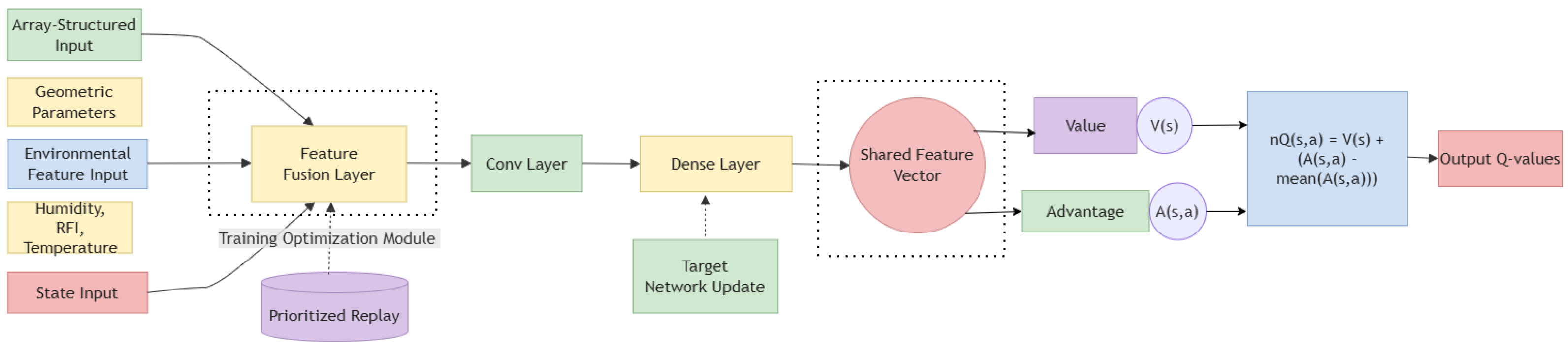
The proposed network architecture takes the state variables defined in Section 3.1 as input, including the normalized ring radii, element activation variables, and ring-level active-element statistics. For the atmospheric-effect setting, the state is further augmented with environmental parameters, namely temperature, humidity, and pressure. These inputs are first passed through a feature-fusion stage and then encoded by a shared fully connected layer with 256 hidden units and ReLU activation, which extracts a compact latent representation for subsequent value and advantage estimation.

The network then branches into two streams. The value stream contains two fully connected layers with 256 hidden units each and ReLU activation, followed by a scalar output that estimates the state-value function $V\left(s\right)$. The advantage stream adopts a similar structure and outputs an $\left|\mathcal{A}\right|$-dimensional vector representing the action-dependent advantage values $A(s,a)$. To improve numerical stability and ensure identifiability, the mean of the advantage values is subtracted before combining the two streams. The final Q-values are computed as

$$Q(s,a)=V\left(s\right)+\left(A(s,a)-{\displaystyle \frac{1}{\left|\mathcal{A}\right|}}\sum _{a^{\prime }}A(s,a^{\prime })\right).$$

(51)

As shown in Figure 2, beyond the classical dueling structure, two additional training mechanisms are incorporated. First, Prioritized Experience Replay is adopted because effective PSLL-improving transitions are relatively sparse during training, and prioritization improves sample efficiency by focusing on informative experiences. Second, a target network updated by hard parameter copying is used to stabilize the temporal-difference learning process [19]. It should be noted that the architecture shown in Figure 2 is not intended to represent the only possible network design. Instead, it is a practical and effective choice tailored to the discrete, constrained optimization problem considered in this work, balancing model complexity, training stability, and computational efficiency.

Figure 2. Architecture of the proposed improved Dueling DQN framework.

As indicated by the dashed box in Figure 2, these modifications improve both convergence stability and training efficiency.

Two-Tier Adaptive Step-Size Strategy for Radius Optimization

To balance exploration and exploitation in ring-radius optimization, we introduce a two-tier adaptive step-size strategy consisting of a global step-size adaptation module (referred to as a “controller” in an algorithmic sense) and a ring-specific refinement mechanism. Here, the term “controller” does not refer to a physical or standard microcontroller, but to an internal rule that dynamically adjusts the optimization step size during the reinforcement-learning process. Compared with a fixed step-size scheme, the proposed strategy improves both convergence efficiency and local-search capability in the minimization of the peak sidelobe level (PSLL).

The global step-size adaptation mechanism adjusts the search granularity according to recent optimization behavior. Let

$$P=\{p_t,p_{t-1},\dots ,p_{t-N+1}\}$$

denote the PSLL sequence over the most recent N optimization steps. The variance

$${\sigma }^2=\mathrm{Var}(\Delta P)$$

and mean

$$\mu =\mathrm{Mean}(\Delta P)$$

are computed from the first-order difference sequence

$$\Delta P=\{p_t-p_{t-1},\dots ,p_{t-N+2}-p_{t-N+1}\}.$$

where ${\sigma }^2$ measures the volatility of recent performance changes, whereas $\mu$ reflects the average trend of the recent PSLL evolution.

Using these statistics and predefined thresholds, the global step size ${\eta }_{\mathrm{global}}$ is adjusted according to the following three cases.

Case 1: Local refinement. If ${\sigma }^2<T_{\mathrm{var}}$ and $\left|\mu \right|<T_{\mathrm{trend}}$, the optimization is regarded as being in a relatively stable region with limited fluctuation. In this case, the step size is reduced for local refinement:

$${\eta }_{\mathrm{global}}\leftarrow \max \left({\eta }_{\min },{\eta }_{\mathrm{global}}·\max \left({\delta }_{\mathrm{decay}},1-\alpha {\sigma }^2\right)\right).$$

(52)

Case 2: Accelerated progress. If ${\sigma }^2\ge T_{\mathrm{var}}$, $\left|\mu \right|\ge T_{\mathrm{trend}}$, and $\mu <0$, the recent updates indicate effective descent. The step size is therefore increased to accelerate exploration:

$${\eta }_{\mathrm{global}}\leftarrow \min \left({\eta }_{\mathrm{init}},{\eta }_{\mathrm{global}}·\min \left(1/{\delta }_{\mathrm{decay}},1+\alpha {\sigma }^2\right)\right).$$

(53)

Case 3: Stabilization under stagnation or degradation. If ${\sigma }^2\ge T_{\mathrm{var}}$, $\left|\mu \right|\ge T_{\mathrm{trend}}$, and $\mu \ge 0$, the search is considered to be unstable or trapped. In this case, the step size is slightly reduced to improve stability:

$${\eta }_{\mathrm{global}}\leftarrow \max \left({\eta }_{\min },{\eta }_{\mathrm{global}}·{\delta }_{\mathrm{decay}}\right).$$

(54)

To avoid prolonged stagnation in local optima, a stagnation-escape mechanism is introduced. When the number of consecutive steps without improvement exceeds a threshold $T_{\mathrm{stagnate}}$, the step size is temporarily amplified as

$${\eta }_{\mathrm{global}}\leftarrow \min \left({\eta }_{\mathrm{init}},{\eta }_{\mathrm{global}}·\left(f_{\mathrm{base}}+f_{\mathrm{scale}}·{\displaystyle \frac{\text{no\_improve\_count}}{T_{\mathrm{stagnate}}}}\right)\right),$$

(55)

after which the stagnation counter is reset.

In addition to the global controller, each ring i is assigned an individual step size ${\eta }_{\mathrm{ring},i}$ to reflect its local sensitivity to PSLL variation. When ring i is updated, the corresponding PSLL improvement is recorded as

$$\Delta p_i=p_{\mathrm{prev}}-p_{\mathrm{current}}.$$

Each ring maintains a history of recent improvements of length M, and the average improvement is denoted by $\Delta {\overline{P}}_i$. For numerical stability, the ring-specific step size is constrained within the interval $[{\eta }_{\mathrm{ring},\min },{\eta }_{\mathrm{ring},\max }]$.

If $\Delta {\overline{P}}_i>0.1$, recent updates on ring i are considered effective, and the step size is enlarged:

$${\eta }_{\mathrm{ring},i}\leftarrow \min \left({\eta }_{\mathrm{ring},\max },{\eta }_{\mathrm{ring},i}·1.1\right).$$

(56)

If $\Delta {\overline{P}}_i<0.02$, recent updates are considered ineffective, and the step size is reduced for finer local adjustment:

$${\eta }_{\mathrm{ring},i}\leftarrow \max \left({\eta }_{\mathrm{ring},\min },{\eta }_{\mathrm{ring},i}·{\delta }_{\mathrm{decay}}\right).$$

(57)

This two-tier strategy enables the search process to adapt to both global optimization trends and local ring-level sensitivities, thereby improving convergence behavior and final solution quality. The values of the thresholds and control parameters, including $T_{\mathrm{var}}$, $T_{\mathrm{trend}}$, $T_{\mathrm{stagnate}}$, $f_{\mathrm{base}}$, $f_{\mathrm{scale}}$, as well as the window sizes N and M, are specified in Appendix A to ensure reproducibility.

5. Simulation Results and Performance Evaluation

5.1. Radius-Only Optimization Using Improved Dueling DQN

Unless otherwise stated, equal-amplitude and in-phase excitation is adopted in all experiments in this section, consistent with the modeling assumptions in Section 3.

We investigate the optimization of ring radii in concentric circular arrays using the improved Dueling DQN framework described in Section 3. The detailed hyperparameter settings are provided in Appendix A to ensure reproducibility. The array under study is a sparse uniform concentric six-ring configuration, consisting of one fixed central element and six independently adjustable rings. The minimum inter-element spacing is constrained to be no less than $0.5\lambda$, and the optimization variables are the six ring radii $R_n$ ($n=1,2,\dots ,6$).

To evaluate robustness and statistical consistency, multiple independent runs with different random initializations are conducted. In this experiment, E1 denotes the baseline DDQN method for radius-only optimization without any of the proposed improvement strategies, while E2 denotes the improved Dueling DQN method with the proposed refinement strategy.

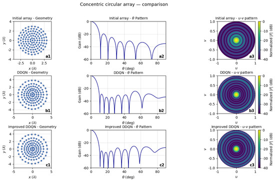
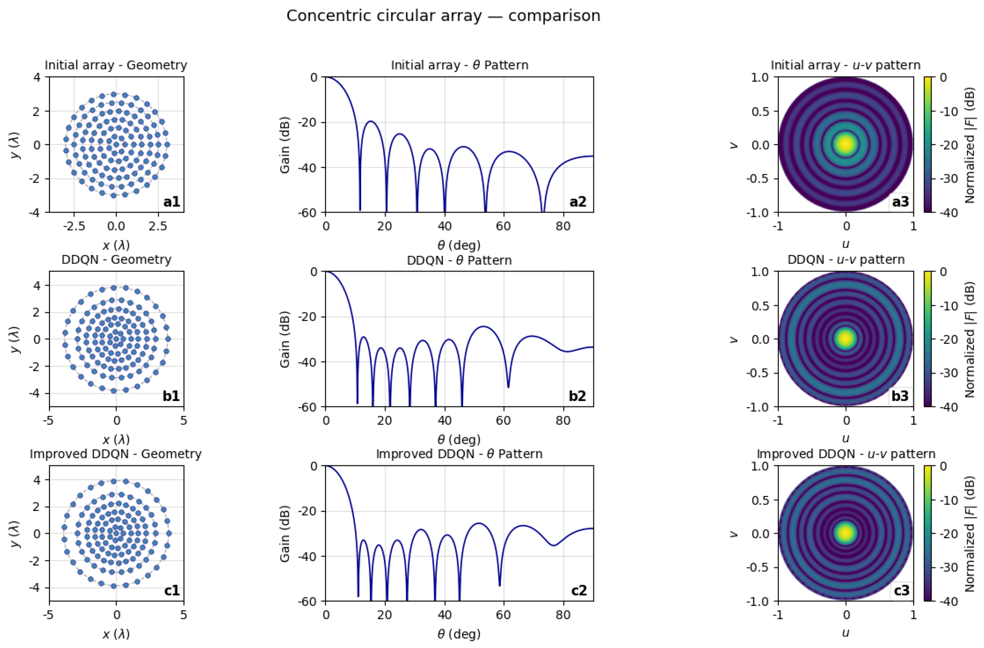
The representative optimized ring radii are summarized in Table 1, and the corresponding array layouts and radiation patterns are illustrated in Figure 3. Specifically, subplots a1–a3 show the initial uniform array, b1–b3 correspond to the baseline DDQN result, and c1–c3 present the result obtained using the improved Dueling DQN.

Table 1. Radius-only optimized array parameters.

Method	PSLL (dB)	${\mathit{R}}_1$	${\mathit{R}}_2$	${\mathit{R}}_3$	${\mathit{R}}_4$	${\mathit{R}}_5$	${\mathit{R}}_6$
Initial array	$-18.672$	0.500000	1.000000	1.500000	2.000000	2.500000	3.000000
DDQN baseline	$-24.0396$	0.520000	1.020000	1.520000	2.201400	2.964200	3.918900
Improved DDQN	$-24.4810$	0.501830	1.022660	1.522660	2.192535	2.958544	3.912160

Figure 3. Radius-only optimization results. Subplots (a1–a3) show the initial uniform array, (b1–b3) show the baseline DDQN-optimized array, and (c1–c3) show the improved Dueling DQN-optimized array.

As shown in Table 1, both DDQN and the proposed method achieve significant sidelobe suppression compared with the initial array, reducing the PSLL from $-18.672$ dB to below $-24$ dB. The best PSLL achieved by the improved method reaches $-24.4810$ dB. Compared with the baseline DDQN result, the proposed method achieves an additional PSLL reduction of approximately $0.44$ dB.

To further evaluate the robustness of the radius-only optimization, statistical results over multiple independent runs are summarized in Table 2. The results show that the proposed method consistently achieves a lower mean PSLL and smaller standard deviation than the baseline DDQN. In particular, the average PSLL is improved from $-23.9892$ dB to $-24.476$ dB, demonstrating a clear performance gain. Moreover, the reduced standard deviation indicates improved stability of the optimization process.

Table 2. Statistical results of radius-only optimization over multiple independent runs.

Setting	Method	Mean PSLL (dB)	Std (dB)	Best (dB)	Worst (dB)
E1	Baseline DDQN	$-23.9892$	0.0329	$-24.0396$	$-23.9406$
E2	Improved DDQN	$-24.476$	0.009	$-24.4810$	$-24.460$

These results indicate that while radius-only optimization can effectively suppress sidelobes, further performance improvements may be achieved by jointly optimizing both the ring radii and the element distribution, which will be investigated in the following section.

In addition, compared with the results reported in [20], the proposed method achieves a further PSLL reduction of approximately $0.31$ dB, demonstrating its competitiveness with existing approaches.

5.2. Concurrent Optimization of Ring Radii and Element Counts

Unless otherwise specified, the equal-amplitude and in-phase excitation assumption is retained in this joint-optimization setting, so that the performance improvement can be attributed to structural optimization rather than excitation reweighting.

Previous single-parameter optimization, which only adjusted the ring radii, suppressed the PSLL to $-24.4810$ dB but did not modify the element distribution density, thereby limiting the ability of sparse arrays to further reduce sidelobes and hardware costs. To address this limitation, an improved Dueling Deep Q-Network (DDQN) framework was employed for joint optimization of ring radii and element counts.

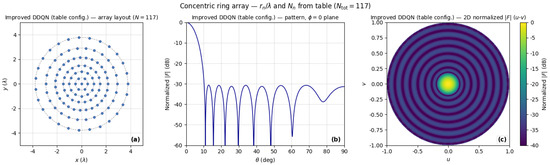
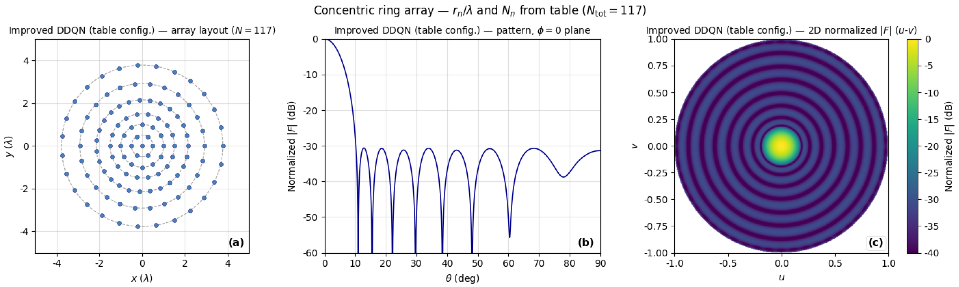
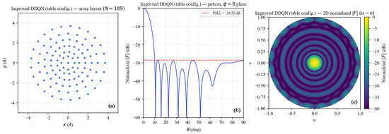
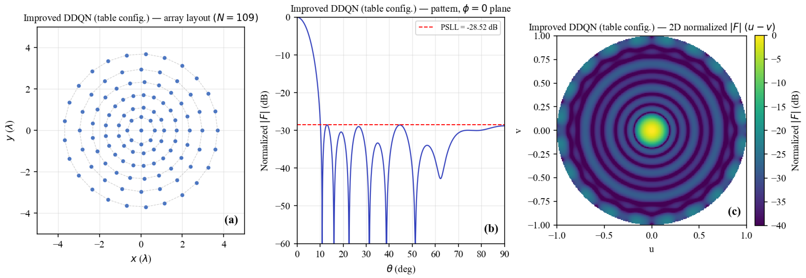
Figure 4 shows the corresponding results obtained using the proposed method. The optimized array configurations are summarized in Table 3. For comparison, a conventional genetic algorithm (GA) was also implemented under the same equal-amplitude and in-phase excitation constraint.

Figure 4. Array layout and corresponding beam-pattern results for the improved DDQN-based joint optimization: (a) array layout; (b) PSLL; (c) three-dimensional beam pattern.

Table 3. Comparison of optimization methods for 6-ring concentric circular arrays.

Method	N	n	1	2	3	4	5	6	PSLL (dB)
Improved DDQN	118	$r_n\left(\lambda \right)$	0.5019	1.0019	1.5019	2.1520	2.9124	3.7751	−30.629
		$N_n$	7	13	19	25	26	27
GA	109	$r_n\left(\lambda \right)$	0.6634	1.1075	1.7172	2.3419	2.9600	3.6999	−28.523
		$N_n$	8	13	21	21	20	25

Figure 5 shows the GA-based design achieves a PSLL of $-28.523$ dB with a total of 109 elements, whereas the proposed improved DDQN method further reduces the PSLL to $-30.629$ dB using 118 elements. Compared with the GA result, the proposed method provides an additional sidelobe reduction of approximately $2.1$ dB, indicating a more effective exploration of the coupled design space of array geometry and sparsity.

Figure 5. Array layout and corresponding beam-pattern results for the GA joint optimization: (a) array layout; (b) PSLL; (c) three-dimensional beam pattern.

Although the proposed method uses a slightly larger number of elements than the GA-based design, the achieved PSLL improvement demonstrates a more efficient utilization of array degrees of freedom through joint structural optimization. This can be attributed to the capability of the DDQN framework to capture long-term reward dependencies and coordinate the interaction between ring spacing and element density across multiple rings.

Moreover, compared with the radius-only optimization, the proposed method achieves a PSLL reduction of $6.148$ dB. These results demonstrate that joint optimization of array geometry and element distribution effectively improves sidelobe suppression while maintaining a reasonable level of hardware complexity.

To further evaluate the effectiveness of the proposed refinement mechanism in the joint optimization framework, we conduct an ablation study by comparing three different configurations:

• E3: Joint optimization without refinement;
• E4: Joint optimization with radius-only refinement;
• E5: Joint optimization with the proposed joint refinement strategy.

All experiments are conducted under the same settings with 10 independent runs to ensure statistical consistency. The corresponding results are summarized in Table 4.

Table 4. Statistical results of joint optimization under different refinement strategies.

Setting	Method	Runs	Mean PSLL (dB)	Std (dB)	Best/Worst (dB)
E3	Joint $r+N$, no refinement	10	−30.312	0.041	−30.361/−30.248
E4	Joint $r+N$, radius-only refinement	10	−30.487	0.052	−30.553/−30.418
E5	Joint $r+N$, joint refinement	10	−30.574	0.038	−30.629/−30.512

As shown in Table 4, introducing refinement improves the optimization performance. Compared with the baseline setting without refinement (E3), the radius-only refinement (E4) achieves a lower mean PSLL, indicating that adaptive adjustment of ring radii contributes to better exploration of the solution space.

The proposed joint refinement strategy (E5) further improves the mean PSLL and achieves the best PSLL of $-30.629$ dB, which is consistent with the optimal result reported in Table 3. This demonstrates that jointly adapting geometric and sparsity-related variables enhances the effectiveness of the optimization process.

In addition, the relatively small standard deviations across all settings indicate stable performance under different random initializations. Overall, the results confirm that the proposed refinement mechanism improves both optimization capability and solution quality in joint array design.

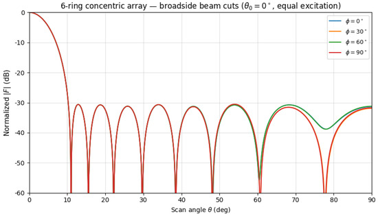
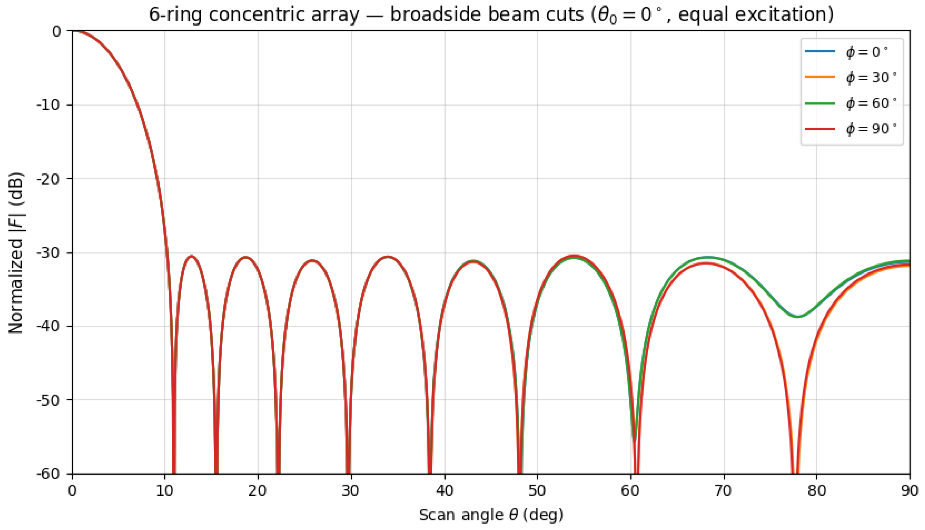
To further examine the azimuthal behavior of the optimized array, beam cuts were evaluated at multiple azimuth angles (0°, 30°, 60°, and 90°). The obtained PSLL values are very close across all directions (approximately $-30.6299$ dB), with only minor variations observed in the far sidelobe region. This near-overlap of beam cuts is expected due to the uniform azimuthal distribution of elements on each ring. Since the optimization process only adjusts ring radii and ring-wise element counts, while the azimuthal positions remain uniformly distributed and are not independently optimized, the resulting radiation pattern naturally exhibits near-rotational symmetry. Therefore, this observation should be interpreted as an inherent structural property of the array configuration rather than a direct consequence of the proposed optimization method. As a result, the beam pattern is largely invariant with respect to azimuth, and a single radial cut can provide a representative characterization of sidelobe performance. As illustrated in Figure 6, the beam cuts at different azimuth angles largely overlap. The small deviations observed in the far sidelobe region do not affect the overall evaluation of array performance.

Figure 6. Beam cuts at different azimuth angles (0°, 30°, 60°, and 90°) for the optimized array. The curves largely overlap, indicating near-rotational symmetry with minor deviations in the far sidelobe region.

5.3. Antenna Arrays Under Tri-Domain Errors and Atmospheric Effects

In this subsection, equal-amplitude and in-phase excitation is also assumed, while stochastic perturbations and atmospheric effects are introduced to evaluate robustness under non-ideal conditions.

To further assess the robustness of the proposed synthesis framework, additional simulations were conducted under tri-domain stochastic disturbances, including element position perturbations, phase jitter, and excitation amplitude fluctuations. These uncertainties introduce phase decorrelation and amplitude imbalance across the array aperture, leading to main-lobe broadening and increased sidelobe levels.

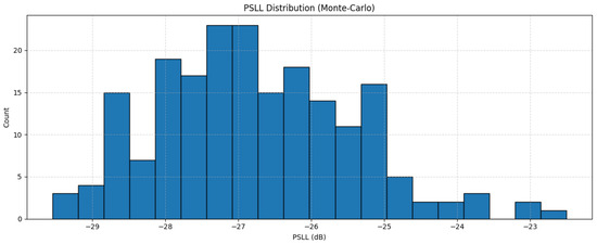
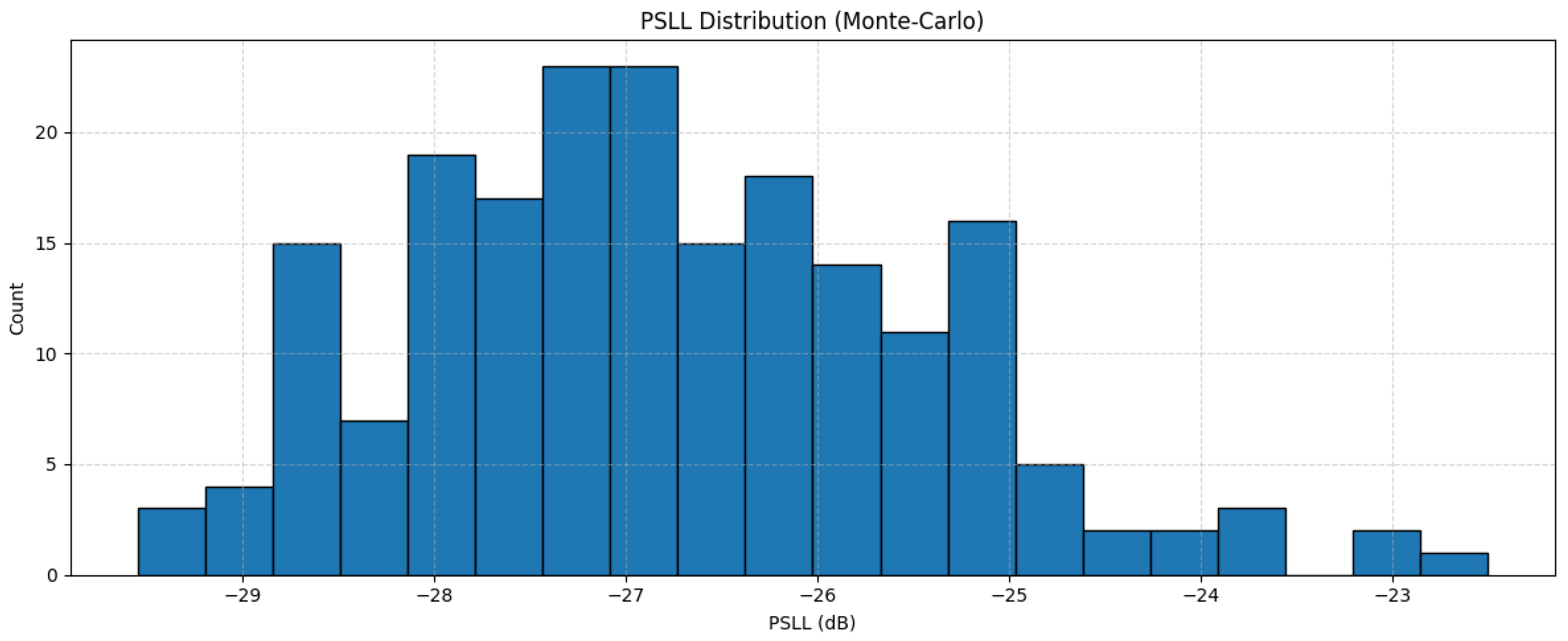
Figure 7 presents the statistical distribution (histogram) of PSLL obtained from 200 Monte Carlo simulations based on repeated perturbations of the same optimized array configuration. Under these conditions, the average PSLL is approximately $-26.758$ dB with a standard deviation of $1.323$ dB. Compared with the ideal (noise-free) case, the PSLL increases by about $3.07$ dB, indicating that tri-domain noise degrades sidelobe suppression performance. Nevertheless, the relatively limited spread of the distribution suggests that the optimized array maintains stable performance under stochastic disturbances.

Figure 7. Histogram of PSLL values obtained from 200 Monte Carlo simulations under tri-domain perturbations.

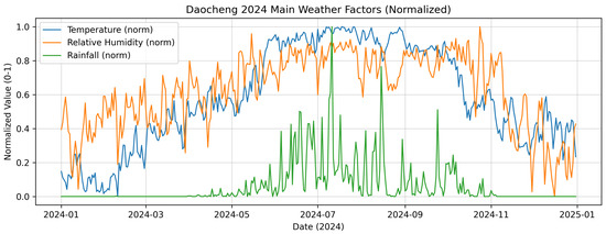
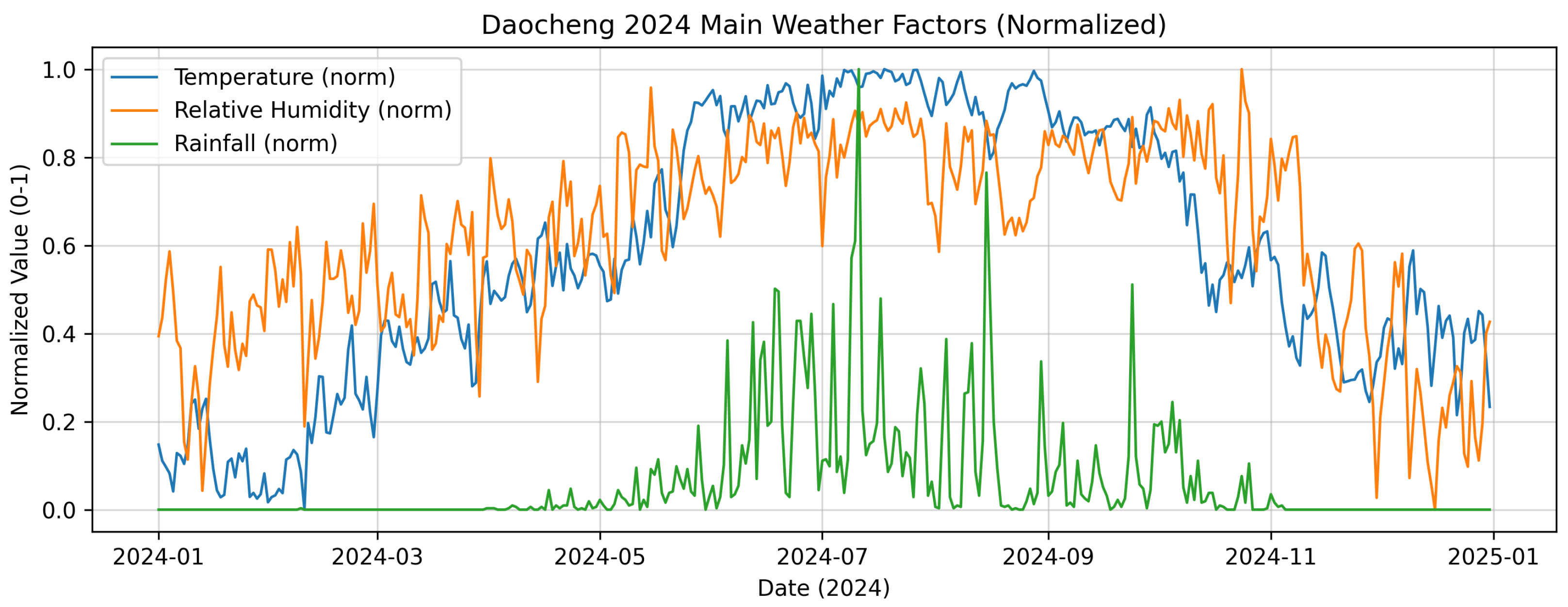
To emulate realistic operating conditions, this study further incorporates daily meteorological data from Daocheng in 2024, including temperature, relative humidity, and rainfall, as shown in Figure 8. Based on the evaluation criteria defined in Section 3, where performance metrics such as PSLL, mainlobe pointing error, and gain loss are jointly considered in the reward formulation, the previously obtained optimized array configuration is selected for further analysis under atmospheric-effect modeling.

Figure 8. Normalized meteorological data in Daocheng during 2024, including temperature, relative humidity, and rainfall.

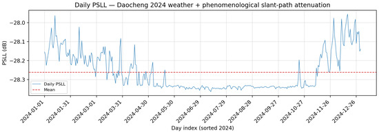
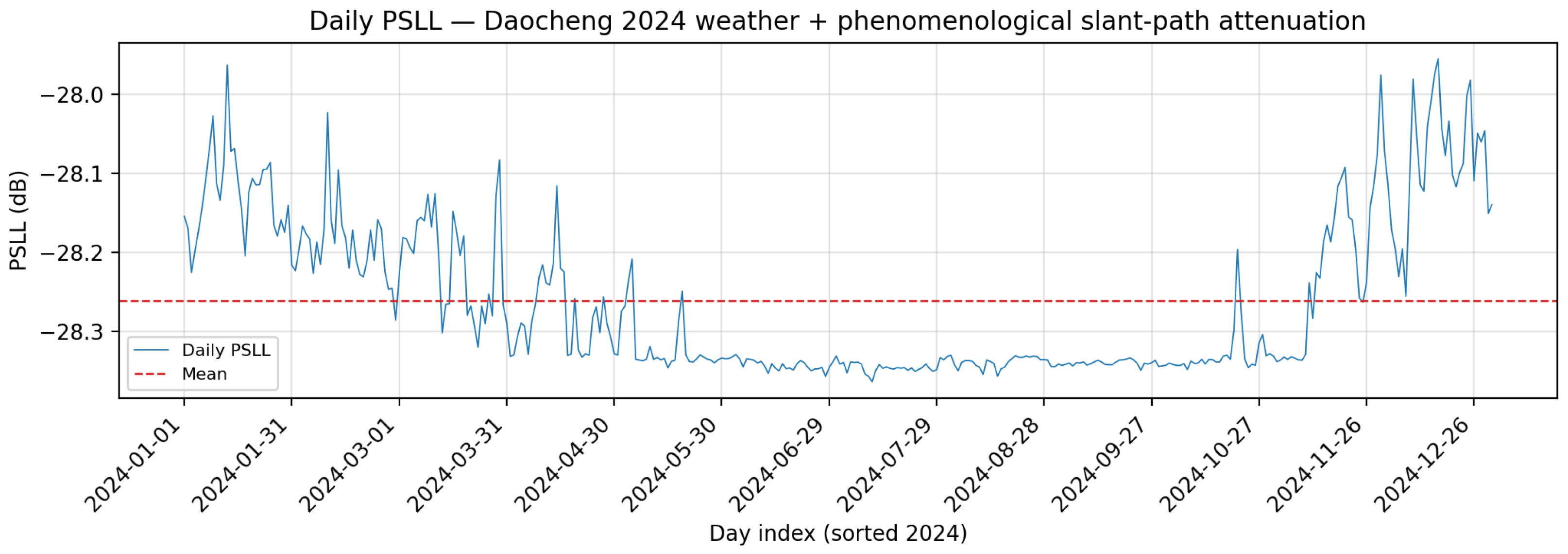
Figure 9 illustrates the temporal variation of PSLL for the selected optimized array configuration under combined tri-domain perturbations and atmospheric effects. Under ideal conditions, the PSLL is approximately $-30.629$ dB. After introducing tri-domain perturbations, the PSLL exhibits a moderate reduction relative to the perturbation-only case. Based on the daily simulation results for Daocheng in 2024, the average PSLL is approximately $-28.261$ dB, corresponding to a reduction of about $1.503$ dB compared with the tri-domain perturbation baseline. The PSLL remains within a narrow range from $-28.363$ dB to $-27.955$ dB throughout the year.

Figure 9. Daily variation of PSLL for the optimized array under atmospheric conditions in Daocheng (2024). The PSLL exhibits limited fluctuation and remains within a narrow range throughout the year.

These results indicate that, under the adopted atmospheric-effect model, propagation-induced attenuation introduces a direction-dependent modification to the normalized beam pattern. In particular, sidelobe regions experience relatively stronger attenuation than the main lobe due to longer effective propagation paths. However, the overall impact remains limited, and atmospheric effects act as a secondary correction rather than a dominant factor in determining PSLL.

Overall, the observed PSLL behavior can be interpreted as the combined effect of stochastic perturbations and propagation-induced attenuation. While tri-domain noise significantly degrades sidelobe performance, atmospheric effects partially compensate for this degradation but do not fundamentally alter the intrinsic characteristics of the optimized array.

6. Discussion

In this work, a co-optimization framework for sparse concentric ring arrays based on an improved Dueling Deep Q-Network (DDQN) is investigated under both ideal and non-ideal conditions. The obtained results provide several insights into the behavior of geometry optimization, sparsity control, and robustness under practical perturbations.

First, the radius-only optimization results demonstrate that adjusting ring radii alone can effectively reduce the peak sidelobe level (PSLL), achieving values below $-24$ dB in all experiments. This improvement can be explained from an aperture-distribution perspective. Modifying the ring radii changes the spatial sampling of the array aperture, which reshapes the interference pattern in the far field. However, since the element counts remain fixed, the degrees of freedom are limited, and the achievable sidelobe suppression is therefore constrained. This explains why the performance gain, although consistent, remains moderate compared with more flexible optimization strategies.

By contrast, the joint optimization of ring radii and element counts introduces additional degrees of freedom, leading to a significant improvement in sidelobe suppression. The proposed method achieves a PSLL of $-30.629$ dB, outperforming both the radius-only optimization and the genetic-algorithm-based design. This performance gain can be attributed to the coupling between geometric spacing and element distribution. While radius adjustment controls the radial layout of the array, element-count optimization modifies the sampling density across different rings, effectively altering the aperture weighting. This joint control enables a more flexible shaping of the sidelobe structure and allows the optimization process to better balance spatial distribution and energy concentration.

The robustness analysis under tri-domain stochastic perturbations further reveals the sensitivity of array performance to practical imperfections. The PSLL increases from approximately $-30.629$ dB to $-26.758$ dB under combined position, phase, and amplitude errors. This degradation can be understood by considering the different roles of these perturbations. Position errors introduce phase deviations in the propagation path, phase errors directly disrupt the coherent superposition of array elements, and amplitude errors modify the effective excitation weights. These effects collectively reduce constructive interference in the main lobe and elevate the sidelobe floor, leading to increased PSLL values [17,18]. Despite this degradation, the relatively small standard deviation observed in Monte Carlo simulations indicates that the optimized array maintains stable performance across different perturbation realizations, suggesting a certain level of inherent robustness in the learned configuration.

The influence of atmospheric effects is further analyzed using real meteorological data. Under the adopted 60 GHz terrestrial propagation model and the considered environmental dataset, the average PSLL is observed to be approximately $-28.261$ dB. Compared with the perturbation-only case, atmospheric effects introduce a moderate variation of about $1.503$ dB. This behavior can be attributed to the fact that atmospheric attenuation primarily acts as a direction-dependent scaling factor on the radiation pattern, rather than fundamentally altering the phase relationships among array elements. Consequently, sidelobe regions, which correspond to longer effective propagation paths, experience slightly stronger attenuation than the main lobe. However, under the present modeling assumptions, the overall impact of atmospheric effects remains smaller than that of stochastic perturbations. It should be emphasized that this observation is dependent on the adopted propagation model and environmental conditions, and may not generalize to all frequency bands or propagation scenarios.

Despite the effectiveness of the proposed framework, several limitations should be noted. First, atmospheric effects are incorporated only in a post-optimization evaluation stage, rather than being included in the optimization loop. Second, the tri-domain error model assumes independent stochastic perturbations and does not consider potential correlations or calibration mechanisms in practical systems. Third, external intentional interference, such as jamming signals, is not modeled in the current framework. These aspects may affect the applicability of the results in more complex electromagnetic environments and should be addressed in future work.

7. Conclusions

In this paper, a co-optimization framework based on an improved Dueling Deep Q-Network is proposed for the design of sparse concentric ring arrays under both ideal and non-ideal conditions. The results show that radius-only optimization provides limited improvement due to restricted degrees of freedom, whereas joint optimization of ring radii and element counts significantly enhances sidelobe suppression, achieving a PSLL of $-30.629$ dB. Furthermore, the optimized array demonstrates stable performance under tri-domain stochastic perturbations, with moderate degradation in sidelobe levels. The analysis of atmospheric effects indicates that, under the adopted propagation model, environmental attenuation introduces only secondary modifications to the normalized radiation pattern. Overall, the proposed method provides an effective and robust approach for sparse array optimization in practical scenarios.

Future work will focus on improving the scalability and computational efficiency of the proposed method, for example by exploring multi-agent reinforcement learning frameworks to decouple continuous and discrete optimization variables, as well as transfer learning strategies to accelerate optimization across different frequency bands. In addition, the framework will be extended toward interference-aware array optimization by incorporating intentional jamming models and learning-based signal classification methods, thereby further enhancing robustness in complex electromagnetic environments.

Appendix A.1. Radius-Only Optimization

Table A1. Dueling DQN hyperparameters for radius-only optimization (phase_a preset).

Hyperparameter	Value	Description
Episodes	2000	Total training episodes
Max steps per episode	100	Maximum environment steps
Batch size	64	Mini-batch size
Replay buffer size	80,000	Experience replay buffer capacity
Learning rate	$5\times {10}^{-4}$	Adam optimizer
Discount factor $\gamma$	0.99	Future reward discount
$\epsilon$-start/end/decay	1.0/0.09/0.9988	$\epsilon$-greedy schedule
Target network update	5 episodes	Hard copy frequency
Hidden layers	2 × 256 units (ReLU)	Dueling DQN architecture
Radius step $\delta r$ (step_lambda)	$0.012\lambda$	Radius adjustment step

Table A1. Dueling DQN hyperparameters for radius-only optimization (phase_a preset).

Hyperparameter	Value	Description
Episodes	2000	Total training episodes
Max steps per episode	100	Maximum environment steps
Batch size	64	Mini-batch size
Replay buffer size	80,000	Experience replay buffer capacity
Learning rate	$5\times {10}^{-4}$	Adam optimizer
Discount factor $\gamma$	0.99	Future reward discount
$\epsilon$-start/end/decay	1.0/0.09/0.9988	$\epsilon$-greedy schedule
Target network update	5 episodes	Hard copy frequency
Hidden layers	2 × 256 units (ReLU)	Dueling DQN architecture
Radius step $\delta r$ (step_lambda)	$0.012\lambda$	Radius adjustment step

Appendix A.2. Joint Radius-and-Count Optimization

Table A2. Dueling DQN hyperparameters for joint radius-and-count optimization (phase_a preset).

Hyperparameter	Value	Description
Episodes	2000	Total training episodes
Max steps per episode	100	Maximum environment steps
Batch size	64	Mini-batch size
Replay buffer size	80,000	Experience replay buffer capacity
Learning rate	$5\times {10}^{-4}$	Adam optimizer
Discount factor $\gamma$	0.99	Future reward discount
$\epsilon$-start/end/decay	1.0/0.09/0.9988	$\epsilon$-greedy schedule
Target network update	5 episodes	Hard copy frequency
Hidden layers	2 × 256 units (ReLU)	Dueling DQN architecture
Radius step $\delta r$	$0.012\lambda$	Radius adjustment step
Max count change $n_{\Delta \max }$	2	$\Delta N\in \{-2,-1,0,+1,+2\}$ per ring

Table A2. Dueling DQN hyperparameters for joint radius-and-count optimization (phase_a preset).

Hyperparameter	Value	Description
Episodes	2000	Total training episodes
Max steps per episode	100	Maximum environment steps
Batch size	64	Mini-batch size
Replay buffer size	80,000	Experience replay buffer capacity
Learning rate	$5\times {10}^{-4}$	Adam optimizer
Discount factor $\gamma$	0.99	Future reward discount
$\epsilon$-start/end/decay	1.0/0.09/0.9988	$\epsilon$-greedy schedule
Target network update	5 episodes	Hard copy frequency
Hidden layers	2 × 256 units (ReLU)	Dueling DQN architecture
Radius step $\delta r$	$0.012\lambda$	Radius adjustment step
Max count change $n_{\Delta \max }$	2	$\Delta N\in \{-2,-1,0,+1,+2\}$ per ring

Appendix A.3. Additional Implementation Details for Reproducibility

To further improve reproducibility, the detailed parameter settings of the proposed adaptive step-size strategy are summarized below.

Global Step-Size Adaptation Parameters:

• Window length for PSLL sequence: $N=10$
• Variance threshold: $T_{\mathrm{var}}=1\times {10}^{-3}$
• Trend threshold: $T_{\mathrm{trend}}=1\times {10}^{-2}$
• Initial global step size: ${\eta }_{\mathrm{init}}=0.012\lambda$
• Minimum global step size: ${\eta }_{\min }=0.002\lambda$
• Decay factor: ${\delta }_{\mathrm{decay}}=0.9$
• Variance scaling factor: $\alpha =0.5$

Stagnation Control Parameters:

• Stagnation threshold: $T_{\mathrm{stagnate}}=50$
• Base amplification factor: $f_{\mathrm{base}}=1.2$
• Scaling factor: $f_{\mathrm{scale}}=0.5$

Ring-Level Adaptation Parameters:

• History length per ring: $M=5$
• Minimum ring step size: ${\eta }_{\mathrm{ring},\min }=0.002\lambda$
• Maximum ring step size: ${\eta }_{\mathrm{ring},\max }=0.02\lambda$
• Enlargement threshold: $\Delta {\overline{P}}_i>0.1$
• Reduction threshold: $\Delta {\overline{P}}_i<0.02$

References

- Thompson, A.R.; Moran, J.M.; Swenson, G.W. Interferometry and Synthesis in Radio Astronomy, 3rd ed.; Springer: Cham, Switzerland, 2017. [Google Scholar]
- Wijnholds, S.J.; Bregman, J.D.; van Ardenne, A. Calibratability and its impact on configuration design for LOFAR and SKA phased array radio telescopes. Radio Sci. 2011, 46, RS0F07. [Google Scholar] [CrossRef] [Scilit]
- Haupt, R.L. Optimized Element Spacing for Low Sidelobe Concentric Ring Arrays. IEEE Trans. Antennas Propag. 2008, 56, 266–268. [Google Scholar] [CrossRef] [Scilit]
- Singh, U.; Kamal, T.S. Synthesis of thinned planar concentric circular antenna arrays using biogeography-based optimization. IET Microw. Antennas Propag. 2012, 6, 822–829. [Google Scholar] [CrossRef] [Scilit]
- Kogan, L. Optimizing a Large Array Configuration to Minimize Side Lobes. IEEE Trans. Antennas Propag. 2000, 48, 1075. [Google Scholar] [CrossRef] [Scilit]
- Boone, F. Interferometric array design: Optimizing the locations of the antenna pads. Astron. Astrophys. 2001, 377, 368–376. [Google Scholar] [CrossRef] [Scilit]
- Boone, F. Interferometric array design: Distributions of Fourier samples for imaging. Astron. Astrophys. 2002, 386, 1160–1171. [Google Scholar] [CrossRef] [Scilit]
- Girard, J.N.; Zarka, P. Towards optimal phased-array tile configurations for large new-generation radio telescopes and their application to NenuFAR. Astron. Astrophys. 2023, 672, A1. [Google Scholar] [CrossRef] [Scilit]
- Xie, H.-H.; Jing, Y.-Q.; Li, Y. Research on Sparse Concentric Ring Array Based on O-1 Programming. Acta Electron. Sin. 2018, 46, 61–67. [Google Scholar] [CrossRef]
- Liu, J.; Liu, J.; Zhao, Z.; Yang, K.; Liu, Q.H. A Hybrid Optimization for Pattern Synthesis of Large Antenna Arrays. IEEE Trans. Antennas Propag. 2014, 145, 81–91. [Google Scholar] [CrossRef] [Scilit]
- Zhao, X.; Zhang, Y.; Yang, Q. Synthesis of Sparse Concentric Ring Arrays Based on Bessel Function. IEEE Trans. Antennas Propag. 2017, 11, 1651–1660. [Google Scholar] [CrossRef] [Scilit]
- Mohammad-Ali-Nezhad, S.; Kassem, M.H. Reinforcement Machine Learning for Sparse Array Antenna Optimization with PPO. Prog. Electromagn. Res. C 2024, 131, 45–60. [Google Scholar] [CrossRef] [Scilit]
- Zheng, Z.; Wu, Q.; Chen, W.; Wu, X.; Zhu, W. Movable Intelligent Surface (MIS) for Wireless Communications: Architecture, Modeling, Algorithm, and Prototyping. IEEE Trans. Wirel. Commun. 2026, 25, 5749–5765. [Google Scholar] [CrossRef] [Scilit]
- Recommendation ITU-R P.676-13; Attenuation by Atmospheric Gases and Related Effects. ITU-R: Geneva, Switzerland, 2022.
- Recommendation ITU-R P.835-6; Reference Standard Atmospheres. ITU-R: Geneva, Switzerland, 2017.
- Recommendation ITU-R P.838-3; Specific Attenuation Model for Rain for Use in Prediction Methods. ITU-R: Geneva, Switzerland, 2005.
- Balanis, C.A. Antenna Theory: Analysis and Design, 3rd ed.; John Wiley & Sons: Hoboken, NJ, USA, 2005. [Google Scholar]
- Van Trees, H.L. Optimum Array Processing; John Wiley & Sons: New York, NY, USA, 2002. [Google Scholar]
- Schaul, T.; Quan, J.; Antonoglou, I.; Silver, D. Prioritized Experience Replay. In Proceedings of the International Conference on Learning Representations (ICLR), San Juan, PR, USA, 2–4 May 2016. [Google Scholar]
- Ni, T.; Wan, T. Design of Concentric Ring Arrays Based on an Adaptive Hybrid Differential Evolution Algorithm. In Proceedings of the 2019 National Conference on Antennas, Kunming, China, 22–25 July 2019; pp. 516–518. [Google Scholar]
Disclaimer/Publisher’s Note: The statements, opinions and data contained in all publications are solely those of the individual author(s) and contributor(s) and not of MDPI and/or the editor(s). MDPI and/or the editor(s) disclaim responsibility for any injury to people or property resulting from any ideas, methods, instructions or products referred to in the content. |
© 2026 by the authors. Licensee MDPI, Basel, Switzerland. This article is an open access article distributed under the terms and conditions of the Creative Commons Attribution (CC BY) license.