LLM-Augmented Ensemble Reasoning for Adversarial-Aware Power Quality Monitoring in Smart Grids

Abstract

Deep learning models for power quality (PQ) disturbance classification remain critically vulnerable to adversarial perturbations, with classification performance degrading severely under white-box attacks. Existing defenses address individual models in isolation and provide no mechanism for operators to assess whether the system is under attack or which classifier remains trustworthy. This paper proposes a two-stage framework that combines adversarial training with large language model (LLM) reasoning to improve both robustness and interpretability. In the first stage, four architecturally diverse classifiers, including a proposed Multi-Scale Temporal Attention Network (MSTAN), are evaluated under four adversarial attacks (FGSM, PGD, C&W, and UAP), and their failure patterns are recorded as structured vulnerability fingerprints. The ensemble is then retrained via adversarial training on mixed clean and perturbed signals. In the second stage, an LLM analyzes the ensemble predictions alongside the fingerprint knowledge base to perform attack detection, fingerprint-guided meta-classification, and operator-facing threat report generation. On a 17-class, 255,000-signal synthetic benchmark, adversarial training recovers FGSM and PGD accuracy from below 25% to the 53–78% range, with MSTAN achieving the highest post-training robustness (78.26% under FGSM, 65.41% under PGD). The LLM reasoning layer provides an additional 3.5–6.2 percentage point improvement over majority voting by selecting the most reliable ensemble member based on the inferred attack condition, and detects adversarial attacks with 87.6% overall accuracy. To our knowledge, this is the first integration of LLM-based ensemble reasoning into the PQ adversarial robustness pipeline and the first application of the C&W optimization attack to power quality signals.

1. Introduction

Power quality (PQ) monitoring is a foundational requirement for the reliable operation of modern electrical networks. The proliferation of nonlinear loads, power electronic converters, and distributed renewable generation has increased both the frequency and the complexity of PQ disturbances, ranging from short-duration impulsive transients to sustained harmonic distortions and compound events involving multiple simultaneous phenomena [1,2]. Accurate classification of these disturbances enables grid operators to diagnose root causes, coordinate protective actions, and maintain supply quality within regulatory limits.

Deep learning has emerged as the dominant approach for automated PQ disturbance classification, with convolutional neural networks [1,3], recurrent architectures [4,5], and hybrid models [6,7] achieving classification accuracies above 97% on standard benchmarks. These results have motivated the deployment of learning-based classifiers in smart grid monitoring infrastructure. However, a growing body of evidence demonstrates that such models are highly susceptible to adversarial perturbations. Tian et al. [8] showed that adding imperceptible noise to PQ signals can reduce classification accuracy from above 92% to below 20%. Alanazi et al. [9] reported accuracy drops of up to 90 percentage points under signal-agnostic adversarial attacks, and documented that each classifier architecture exhibits distinct, predictable failure patterns under attack. Zhang et al. [10,11] further demonstrated that momentum-based iterative attacks and their variants pose persistent threats to CNN-LSTM classifiers used in PQ systems. These findings raise a fundamental concern: deploying deep learning for PQ classification without addressing adversarial robustness introduces a concrete cybersecurity risk to critical power infrastructure.

Existing defenses against adversarial attacks in the PQ domain have focused primarily on adversarial training [8,10], in which models are retrained on mixtures of clean and perturbed signals, and on preprocessing-based approaches such as denoising autoencoders [7] and generative adversarial reconstruction [12]. While these methods recover a meaningful portion of the lost accuracy, they share two structural limitations. First, they operate on individual models in isolation: each classifier is defended independently, with no mechanism to exploit the diversity of an ensemble when multiple architectures are available. Second, they provide no interpretability: the defended model outputs a class label, but the operator receives no information about whether the system is under attack, which model is most trustworthy, or what action should be taken. In safety-critical power system environments, this lack of transparency limits operator trust and hinders real-world adoption [13].

Large language models (LLMs) have recently been explored as reasoning and explanation tools in power system applications, including dispatch optimization [14], security monitoring [15], and cyberattack explanation [13]. Sharshar et al. [13] demonstrated that an LLM can interpret ML classifier outputs and generate structured explanations for false data injection attacks in automatic generation control systems, achieving 93% accuracy in identifying the attack target when provided with appropriate few-shot context. However, their framework addresses a binary detection task in a different domain (AGC frequency signals) and does not involve ensemble reasoning, multi-class PQ classification, or attack-type identification from prediction patterns.

This paper proposes a two-stage framework that addresses both limitations identified above. In the first stage, four architecturally diverse classifiers are evaluated under four adversarial attacks, their model-specific failure patterns are recorded as structured vulnerability fingerprints, and the ensemble is retrained via adversarial training. In the second stage, a large language model receives the ensemble predictions together with the fingerprint knowledge base and performs three reasoning tasks: assessing whether the system is under adversarial attack and inferring the attack type, selecting the most reliable ensemble member for the final classification, and generating a structured threat report for the grid operator.

The principal contributions of this work are as follows:

• A two-stage framework that combines adversarial training at the model level with LLM-based reasoning at the prediction level. The two defense mechanisms are complementary, and together they yield compounding accuracy improvements.
• A novel temporal classification architecture, the Multi-Scale Temporal Attention Network (MSTAN), which integrates parallel multi-scale convolution, dilated causal convolution, and temporal self-attention for PQ disturbance classification.
• The first application of the Carlini and Wagner (C&W) attack [16] to power quality signals, extending the adversarial evaluation landscape for PQ classification beyond gradient-sign and universal perturbation methods.
• The first integration of LLM-based reasoning into the PQ adversarial robustness pipeline, enabling zero-shot attack detection, fingerprint-guided meta-classification, and interpretable threat report generation from ensemble prediction patterns.
• A comprehensive adversarial benchmark spanning four models and four attacks (FGSM [17], PGD [18], C&W [16], UAP [19]), providing 16 pre-training and 20 post-training evaluation scenarios on a publicly available 17-class, 255,000-signal dataset [8].

The remainder of this paper is organized as follows. Section 2 reviews related work on PQ classification, adversarial attacks and defenses, and LLMs in power systems. Section 3 presents the proposed framework, including the MSTAN architecture, attack formulations, fingerprint construction, and LLM reasoning pipeline. Section 4 describes the experimental setup. Section 5 reports and discusses the results. Section 6 concludes the paper.

2. Related Work

2.1. Power Quality Disturbance Classification

Accurate classification of power quality disturbances (PQDs) is essential for maintaining grid stability and protecting sensitive equipment. Traditional approaches rely on signal processing transforms, including the discrete Fourier transform [20], wavelet packet decomposition [21], the S-transform [3,22], and Hilbert-Huang analysis [23], to extract handcrafted features from voltage and current waveforms. Although effective under controlled conditions, these methods require substantial domain expertise and degrade when noise or superimposed disturbances are present [7].

Deep learning has since enabled automatic feature extraction from raw signals. Convolutional neural networks (CNNs) achieve above 97% accuracy on standard PQD benchmarks [1,2]. Recurrent architectures, including long short-term memory (LSTM) networks [4,24] and gated recurrent units (GRUs) [5,6], further capture temporal dynamics of disturbance events. Hybrid pipelines that combine spectral preprocessing with sequential classifiers have shown particular resilience to noise. Janthong et al. [7] coupled a denoising autoencoder with a GRU operating on power spectra, sustaining 85.6% accuracy at 5 dB signal-to-noise ratio across 16 triple-disturbance classes. Attention mechanisms have also proven effective: Alanazi et al. [9] embedded a temporal attention layer within a convolutional backbone and reported 97.63% clean accuracy on 17 IEEE 1159-compliant classes.

2.2. Adversarial Attacks on Power Quality Systems

Deep neural networks are susceptible to adversarial perturbations, i.e., imperceptible input modifications that induce systematic misclassification [17]. In computer vision, gradient-based attacks such as the fast gradient sign method (FGSM) [17], projected gradient descent (PGD) [18], and the Carlini–Wagner (C&W) optimization attack [16] have been studied extensively. Universal perturbation methods that craft a single input-agnostic vector applicable to any sample have also been proposed [19].

Within the power quality domain, Tian et al. [8] first adapted signal-specific and signal-agnostic adversarial attacks to CNN-based PQD classifiers, revealing accuracy collapses from above 92% to below 10% under white-box conditions. Zhang et al. [10] subsequently proposed the momentum-iterative FGSM (MI-FGSM) for PQD classification and showed that momentum stabilization produces smaller yet more effective perturbations than single-step methods. A follow-up study introduced the variance-tuned variant (VMI-FGSM) for black-box settings and paired it with a generative adversarial defense [12]. Zhang et al. [11] further evaluated four representative attacks (FGSM, its variant, PGD, and the signal-specific adversarial attack) and proposed a multi-source feature detector to identify adversarial inputs before they reach the classifier.

Alanazi et al. [9] extended this line of inquiry through vulnerability fingerprinting, demonstrating that each architecture exhibits distinct misclassification patterns under attack. Their analysis showed that ResNet collapsed entirely into a single target class, while VGG16 concentrated over 91% of its errors into another. Adjacent power system applications have also been targeted, including state estimation [25], load forecasting [26], and non-intrusive load monitoring [27].

2.3. Defense Mechanisms and Robustness

Adversarial training, in which models are retrained on mixtures of clean and perturbed examples, is the primary defense explored in the PQD domain. Tian et al. [8] showed that this strategy partially recovers classification accuracy. Alanazi et al. [9] quantified the robustness–accuracy tradeoff, reporting 95.91% clean accuracy retention after adversarial training with up to 72.94% accuracy under FGSM. Zhang et al. [10] proposed iterative adversarial training to handle multiple perturbation strengths, while [11] introduced a multi-source feature adversarial training algorithm that mitigates the clean-data accuracy degradation commonly observed with standard adversarial training.

Outside the PQD domain, ensemble diversity is an established complementary robustness mechanism. Tramèr et al. [28] demonstrated that training on adversarial examples transferred from other models decouples the defender from a single attack source. Ensemble defense frameworks combining multiple strategies have been applied to intrusion detection systems [29], and dynamic model selection that varies the active classifier at inference time has been investigated to prevent attackers from reliably computing gradients [30].

2.4. Large Language Models in Power Systems

LLMs have been explored for several power system tasks, including fault diagnosis, load forecasting, and dispatch optimization [31]. Cheng et al. [14] developed GAIA, a domain-specific LLM fine-tuned for power dispatch that translates operator instructions into control actions. An LLM-based monitoring framework by [15] integrated prompt engineering with fuzzy evaluation to produce quantitative security scores on the IEEE 14-bus system.

Sharshar et al. [13] proposed a hybrid framework pairing a gradient-boosted classifier with GPT-4o mini to detect and explain false data injection attacks in automatic generation control (AGC) systems, achieving 93% accuracy in identifying attack targets from structured signal metadata. Their framework, however, operates on frequency regulation signals rather than PQD waveforms, relies on a single detection model instead of a diverse ensemble, and does not address adversarial evasion attacks.

Despite the progress outlined above, several limitations persist across the literature. Most PQD classification studies evaluate robustness only against Gaussian noise and do not consider adversarial perturbations [1,2,7]. Among those that do, attack evaluations are confined to gradient-based methods (FGSM, PGD, MI-FGSM); the Carlini–Wagner optimization attack, which routinely defeats defenses that withstand gradient-based perturbations, has never been applied to power quality signals [9,10,11]. Architecturally, existing adversarial studies test at most two to three models drawn from a single family (CNN, VGG, ResNet), leaving multi-scale, dilated, and transformer-based classifiers unexamined under adversarial conditions [8,9]. Defense mechanisms remain static: the same model and decision rule are applied regardless of attack type, with no capacity to detect which attack is active or to adjust trust across ensemble members accordingly [9,11]. Furthermore, no prior work provides interpretable, operator-facing explanations of adversarial threats in PQD monitoring, despite the critical nature of grid infrastructure [13,31]. This paper therefore proposes a multi-scale temporal attention network (MSTAN) evaluated alongside three diverse baselines under four attack types, including C&W. The framework incorporates an LLM-augmented ensemble reasoning layer that detects the active attack, dynamically adjusts model trust based on empirically derived vulnerability fingerprints, and generates interpretable threat assessments for grid operators.

3. Materials and Methods

3.1. Overview

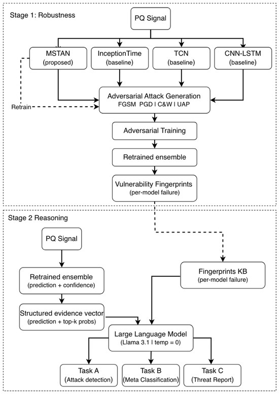
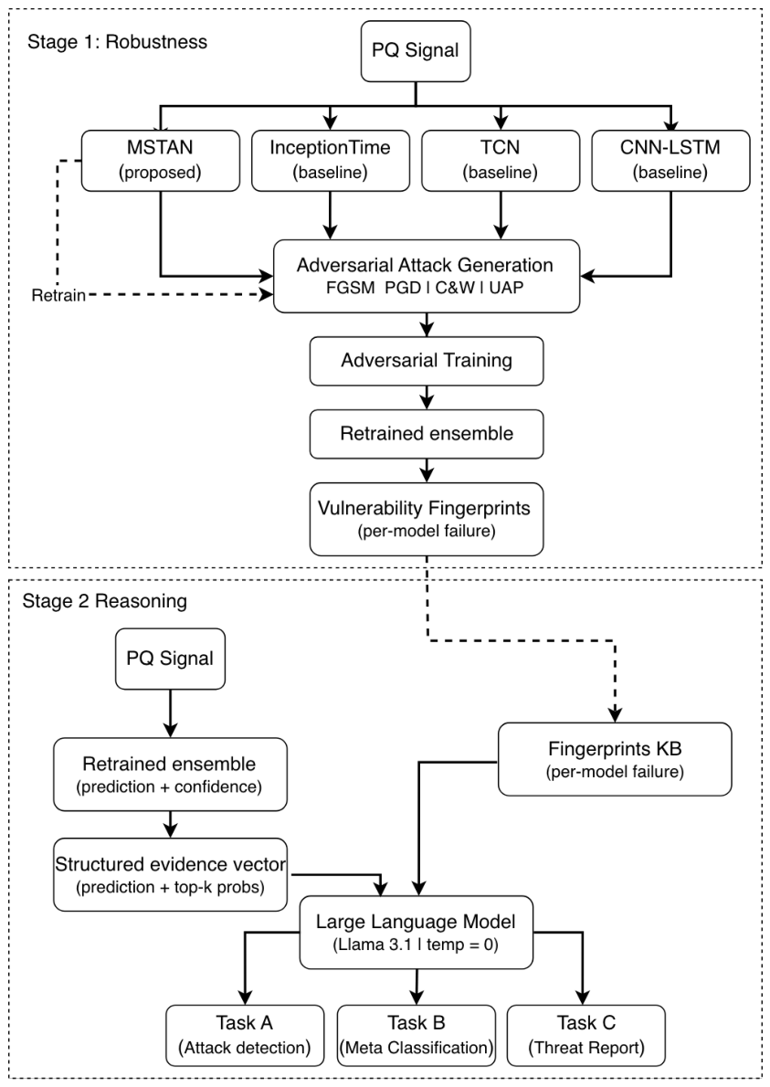
The proposed framework operates in two stages: a robustness stage that improves the adversarial resilience of an ensemble of diverse classifiers through adversarial training, and a reasoning stage that employs a large language model to identify potential attacks, improve classification under adversarial conditions, and generate interpretable threat assessments for grid operators. Figure 1 illustrates the complete pipeline.

Figure 1. Overview of the proposed two-stage framework. Stage 1 trains four architecturally diverse classifiers on clean data, evaluates their robustness under four adversarial attacks, extracts per-model vulnerability fingerprints, and retrains the ensemble via adversarial training. Stage 2 assembles the ensemble predictions into a structured evidence vector and passes it, together with the fingerprint knowledge base, to a large language model that performs attack detection (Task A), meta-classification (Task B), and threat report generation (Task C).

In the robustness stage, a raw power quality signal is simultaneously processed by four architecturally diverse classifiers: the proposed Multi-Scale Temporal Attention Network (MSTAN), InceptionTime, a Temporal Convolutional Network (TCN), and a CNN-LSTM. Each model is first trained on clean data, then subjected to four adversarial attacks (FGSM, PGD, C&W, and UAP) to characterize their failure modes. The resulting failure patterns are recorded as a structured vulnerability fingerprint for each model–attack pair. All four models are subsequently retrained via adversarial training, which augments the training set with adversarially perturbed examples to improve robustness.

In the reasoning stage, the adversarially trained ensemble processes each incoming signal, and the four models’ predictions, confidence scores, and top-k class probabilities are assembled into a structured evidence vector. This evidence, together with the precomputed vulnerability fingerprints, is passed to a large language model that performs three tasks in sequence. First, it analyzes a batch of recent evidence vectors to assess whether the system is under adversarial attack and, if so, infers the attack type (Task A: Attack Detection). Second, it produces the final classification by selecting the most reliable ensemble member based on the detected attack condition and the corresponding fingerprint entries (Task B: Meta-Classification). Third, it synthesizes the detection and classification outputs into a structured natural-language report for the grid operator (Task C: Threat Report Generation). The following subsections formalize each component.

3.2. Multi-Scale Temporal Attention Network

MSTAN takes as input a raw one-dimensional power quality signal $\mathbf{x}\in {\mathbb{R}}^{N\times 1}$, where $N=640$ samples span ten cycles of the 50 Hz fundamental at a 3200 Hz sampling rate. Four components are applied in sequence: multi-scale parallel convolution for local feature extraction at multiple resolutions, dilated causal convolution for capturing longer temporal context, temporal self-attention for focusing on disturbance-bearing segments, and a classification head that maps the resulting representation to 17 disturbance classes. Algorithm 1 summarizes the forward computation.

3.2.1. Multi-Scale Parallel Convolution

Power quality disturbances exhibit a broad range of temporal extents. Impulsive transients may last only one or two samples, whereas voltage sags and flicker persist over hundreds of samples. Motivated by the multi-resolution design of Inception modules [32,33], the first block applies four parallel one-dimensional convolutions with kernel sizes $k\in \{3,7,15,31\}$. Each branch produces 32 feature maps:

$${\mathbf{h}}^{\left(k\right)}=\mathrm{ReLU}\left(\mathrm{BN}\left({\mathbf{W}}^{\left(k\right)}\ast \mathbf{x}+{\mathbf{b}}^{\left(k\right)}\right)\right),k\in \{3,7,15,31\}$$

(1)

where ∗ is the one-dimensional convolution operator, ${\mathbf{W}}^{\left(k\right)}$ and ${\mathbf{b}}^{\left(k\right)}$ are learnable parameters, and BN denotes batch normalization [34]. Concatenating the four outputs along the channel axis yields a 128-channel tensor ${\mathbf{H}}_{\mathrm{ms}}=[{\mathbf{h}}^{\left(3\right)};{\mathbf{h}}^{\left(7\right)};{\mathbf{h}}^{\left(15\right)};{\mathbf{h}}^{\left(31\right)}]$. A subsequent $1\times 1$ pointwise convolution projects this tensor to 64 channels, reducing the computational burden on downstream layers while preserving the fused multi-scale information.

3.2.2. Dilated Causal Convolution

Once multi-scale local features have been extracted, the network requires a mechanism to relate them across longer temporal spans. Dilated causal convolutions [35,36] achieve this by exponentially increasing the receptive field without adding parameters. Three causal convolutional layers with dilation factors $d\in \{1,2,4\}$ and 128 filters per layer are stacked:

$${\mathbf{g}}_t^{\left(d\right)}=\mathrm{ReLU}\left(\mathrm{BN}\left({\displaystyle \sum _{i=0}^{k-1}}{\mathbf{W}}_i^{\left(d\right)}{\mathbf{z}}_{t-d·i}+{\mathbf{b}}^{\left(d\right)}\right)\right)$$

(2)

where ${\mathbf{z}}_t$ denotes the input at time step t and $k=3$ is the kernel size. A single stack of three layers with dilation rates 1, 2, and 4 covers an effective receptive field of 15 time steps. Two such stacks are applied in succession, extending coverage to 29 time steps. Following the residual learning principle [37], a skip connection spans each stack:

$${\mathbf{z}}_{\mathrm{out}}=\mathrm{Dropout}\left({\mathbf{g}}^{(d=4)}\right)+{\mathbf{z}}_{\mathrm{in}}$$

(3)

This residual path stabilizes gradient flow through the deeper layers and retains the original temporal structure of the signal.

3.2.3. Temporal Self-Attention

Not all temporal segments of a power quality signal contribute equally to classification. The region containing the disturbance carries most of the discriminative information, while normal-state portions offer little value. A scaled dot-product self-attention layer [38] is therefore placed after the dilated convolution block so that the network can learn to weight informative segments more heavily.

Given the feature matrix $\mathbf{Z}\in {\mathbb{R}}^{T\times D}$, where T is the number of temporal positions and D the feature dimensionality, query, key, and value matrices are obtained through linear projections:

$$\mathbf{Q}=\mathbf{Z}{\mathbf{W}}_Q,\mathbf{K}=\mathbf{Z}{\mathbf{W}}_K,\mathbf{V}=\mathbf{Z}{\mathbf{W}}_V$$

(4)

with ${\mathbf{W}}_Q,{\mathbf{W}}_K,{\mathbf{W}}_V\in {\mathbb{R}}^{D\times D}$. The attention-weighted context is then:

$$\mathbf{A}=\mathrm{softmax}\left({\displaystyle \frac{\mathbf{Q}{\mathbf{K}}^{\top }}{\sqrt{D}}}\right),\mathbf{C}=\mathbf{A}\mathbf{V}$$

(5)

Each entry $A_{ij}$ captures how relevant time step j is to time step i, allowing the network to attend to disturbance-active regions while suppressing uninformative segments. The resulting context matrix $\mathbf{C}\in {\mathbb{R}}^{T\times D}$ is passed to the classification head.

3.2.4. Classification Head

Global average pooling [39] aggregates $\mathbf{C}$ along the temporal axis, producing a fixed-length vector regardless of signal duration. Two fully connected layers with ReLU activations and dropout regularization [40] map this vector to the output space:

$$\widehat{\mathbf{y}}=\mathrm{softmax}\left({\mathbf{W}}_2\mathrm{ReLU}\left({\mathbf{W}}_1\mathrm{GAP}\left(\mathbf{C}\right)+{\mathbf{b}}_1\right)+{\mathbf{b}}_2\right)$$

(6)

where ${\mathbf{W}}_1\in {\mathbb{R}}^{256\times D}$ and ${\mathbf{W}}_2\in {\mathbb{R}}^{17\times 128}$, and dropout rates of 0.5 and 0.3 are applied after the first and second layers, respectively. The network is trained end-to-end by minimizing the categorical cross-entropy loss:

$${\mathcal{L}}_{\mathrm{CE}}=-{\displaystyle \frac{1}{M}}{\displaystyle \sum _{i=1}^M}{\displaystyle \sum _{j=1}^C}{y}_{i,j}log{\widehat{y}}_{i,j}$$

(7)

where M is the number of training samples, $C=17$ is the number of classes, $y_{i,j}$ is the ground-truth indicator, and ${\widehat{y}}_{i,j}$ is the predicted probability for sample i and class j. Optimization is performed using the Nadam optimizer [41] with an initial learning rate of 0.002.

Algorithm 1 MSTAN Forward Computation.

Require: Raw PQ signal $\mathbf{x}\in {\mathbb{R}}^{N\times 1}$ Ensure: Predicted class probabilities $\widehat{\mathbf{y}}\in {\mathbb{R}}^C$   1: // Multi-Scale Parallel Convolution   2: for each kernel size $k\in \{3,7,15,31\}$ do   3:     ${\mathbf{h}}^{\left(k\right)}\leftarrow \mathrm{ReLU}\left(\mathrm{BN}\left(\mathrm{Conv}1\mathrm{D}(\mathbf{x},k,32\mathrm{filters})\right)\right)$   4: end for   5: ${\mathbf{H}}_{\mathrm{ms}}\leftarrow \mathrm{Concat}({\mathbf{h}}^{\left(3\right)},{\mathbf{h}}^{\left(7\right)},{\mathbf{h}}^{\left(15\right)},{\mathbf{h}}^{\left(31\right)})$                                  ▹ 128 channels   6: $\mathbf{z}\leftarrow \mathrm{Conv}1\mathrm{D}({\mathbf{H}}_{\mathrm{ms}},k=1,64\mathrm{filters})$                                             ▹ Bottleneck   7: // Dilated Causal Convolution (2 stacked blocks)   8: for block $=1,2$ do   9:     ${\mathbf{z}}_{\mathrm{in}}\leftarrow \mathbf{z}$ 10:     for each dilation factor $d\in \{1,2,4\}$ do 11:         $\mathbf{z}\leftarrow \mathrm{ReLU}\left(\mathrm{BN}\right(\mathrm{CausalConv}1\mathrm{D}(\mathbf{z},d,128\mathrm{filters})\left)\right)$ 12:     end for 13:     $\mathbf{z}\leftarrow \mathrm{Dropout}\left(\mathbf{z}\right)+{\mathbf{z}}_{\mathrm{in}}$                                       ▹ Residual connection 14: end for 15: // Temporal Self-Attention 16: $\mathbf{Q},\mathbf{K},\mathbf{V}\leftarrow \mathbf{z}{\mathbf{W}}_Q,\mathbf{z}{\mathbf{W}}_K,\mathbf{z}{\mathbf{W}}_V$ 17: $\mathbf{A}\leftarrow \mathrm{softmax}(\mathbf{Q}{\mathbf{K}}^{\top }/\sqrt{D})$ 18: $\mathbf{C}\leftarrow \mathbf{A}\mathbf{V}$ 19: // Classification Head 20: $\mathbf{v}\leftarrow \mathrm{GAP}\left(\mathbf{C}\right)$                                            ▹ Global average pooling 21: $\widehat{\mathbf{y}}\leftarrow \mathrm{softmax}({\mathbf{W}}_2\mathrm{ReLU}({\mathbf{W}}_1\mathbf{v}+{\mathbf{b}}_1)+{\mathbf{b}}_2)$ 22: return  $\widehat{\mathbf{y}}=0$

3.3. Adversarial Attack Formulation

To evaluate the robustness of each classifier and to construct the vulnerability fingerprints used in Stage 2, four adversarial attack methods are applied. These span a range of threat models: single-step versus iterative, ${\ell }_{\infty }$ versus ${\ell }_2$ bounded, and input-specific versus universal. All perturbations are crafted in the white-box setting, where the attacker has full access to the target model’s parameters and gradients.

3.3.1. Fast Gradient Sign Method (FGSM)

FGSM [17] generates an adversarial example in a single gradient step by perturbing the input along the sign of the loss gradient:

$${\mathbf{x}}_{\mathrm{adv}}=\mathbf{x}+ϵ·\mathrm{sign}\left({\nabla }_{\mathbf{x}}\mathcal{L}(\mathbf{x},y;\theta )\right)$$

(8)

where $\mathbf{x}$ is the clean signal, y is the true label, $\theta$ denotes the model parameters, $\mathcal{L}$ is the cross-entropy loss, and $ϵ$ controls the perturbation magnitude under the ${\ell }_{\infty }$ norm. FGSM serves as a computationally inexpensive baseline that tests a model’s sensitivity to small, worst-case gradient-aligned perturbations.

3.3.2. Projected Gradient Descent (PGD)

PGD [18] extends FGSM into an iterative procedure that applies multiple smaller gradient steps with random initialization:

$${\mathbf{x}}_{\mathrm{adv}}^{(t+1)}={\mathsf{\Pi }}_{{\mathcal{B}}_{ϵ}\left(\mathbf{x}\right)}\left({\mathbf{x}}_{\mathrm{adv}}^{\left(t\right)}+\alpha ·\mathrm{sign}\left({\nabla }_{\mathbf{x}}\mathcal{L}({\mathbf{x}}_{\mathrm{adv}}^{\left(t\right)},y;\theta )\right)\right)$$

(9)

where $\alpha$ is the step size, t indexes the iteration, and ${\mathsf{\Pi }}_{{\mathcal{B}}_{ϵ}\left(\mathbf{x}\right)}$ projects the perturbed signal back onto the ${\ell }_{\infty }$ ball of radius $ϵ$ centered at $\mathbf{x}$. PGD is widely regarded as a strong first-order adversary and provides a more thorough exploration of the perturbation space than FGSM [18].

3.3.3. Carlini and Wagner (C&W) Attack

The C&W attack [16] formulates adversarial example generation as a constrained optimization problem that minimizes the ${\ell }_2$ distance between the clean and adversarial signals while forcing a misclassification:

$$\underset{\mathit{\delta }}{min}{\parallel \mathit{\delta }\parallel }_2^2+c·f(\mathbf{x}+\mathit{\delta })$$

(10)

where $\mathit{\delta }$ is the perturbation, $c>0$ is a regularization constant found through binary search, and $f(·)$ is an objective function defined as:

$$f\left({\mathbf{x}}^{\prime }\right)=max\left(Z{\left({\mathbf{x}}^{\prime }\right)}_y-\underset{j\ne y}{max}Z{\left({\mathbf{x}}^{\prime }\right)}_j,-\kappa \right)$$

(11)

Here, $Z{\left({\mathbf{x}}^{\prime }\right)}_j$ denotes the logit output for class j, y is the true class, and $\kappa \ge 0$ is a confidence margin. To our knowledge, no prior work has applied the C&W attack to power quality signals. Its inclusion allows us to assess classifier robustness against an optimization-based adversary that produces minimal, perceptually subtle perturbations, complementing the gradient-sign attacks above. Due to the iterative optimization involved, C&W is evaluated on a randomly sampled subset of 5000 signals per model, a common practice for computationally expensive attacks [16]. The attack operates in the normalized signal space (zero mean and unit variance), matching the input representation used by the classifiers. Unlike the ${\ell }_{\infty }$-bounded FGSM and PGD attacks, C&W does not apply gradient-sign clipping or projection onto an $ϵ$-ball; the perturbation magnitude is instead governed by the regularization constant c, located through binary search, which trades off the ${\ell }_2$ distortion against the misclassification objective in Equation (10). An attack is counted as successful when a signal that was correctly classified before perturbation is misclassified afterward, consistent with the attack success rate in Equation (17).

3.3.4. Universal Adversarial Perturbation (UAP)

Unlike the input-specific methods above, UAP [19] seeks a single perturbation vector ${\mathit{\delta }}_u$ that, when added to any input, causes misclassification with high probability:

$${\mathit{\delta }}_u=arg\underset{\mathit{\delta }}{min}{\parallel \mathit{\delta }\parallel }_p\mathrm{s}.\mathrm{t}.{\displaystyle \frac{1}{\left|\mathcal{X}\right|}}\sum _{\mathbf{x}\in \mathcal{X}}\mathbb{1}\left[f(\mathbf{x}+\mathit{\delta })\ne f\left(\mathbf{x}\right)\right]\ge 1-\xi$$

(12)

where $\mathcal{X}$ is a set of training signals, $f(·)$ returns the predicted label, $\xi$ is the desired fooling rate threshold, and ${\parallel ·\parallel }_p$ constrains the perturbation under the chosen norm. UAP is constructed iteratively: for each signal that is still correctly classified, the minimum perturbation required to cross the nearest decision boundary is computed and accumulated into ${\mathit{\delta }}_u$ [19]. From a deployment perspective, UAP represents a realistic threat because the attacker needs to craft the perturbation only once and can apply it universally without knowledge of individual inputs at inference time.

Table 1 in Section 4 reports the specific parameter settings ($ϵ$, $\alpha$, iteration count, c, $\kappa$, $\xi$) used for each attack.

Table 1. Adversarial attack parameters.

Attack	Parameter	Symbol	Value
FGSM	Perturbation bound	$ϵ$	0.03, 0.05, 0.1
PGD	Perturbation bound	$ϵ$	0.03, 0.05, 0.1
	Step size	$\alpha$	$ϵ/10$
	Iterations		40
C&W	Confidence margin	$\kappa$	0
	Binary search steps		9
	Optimization steps		1000
UAP	Perturbation norm	${\parallel \mathit{\delta }\parallel }_{\infty }$	0.1
	Fooling rate threshold	$\xi$	0.8

3.4. Vulnerability Fingerprint Construction

Each classifier in the ensemble responds differently to each attack type. A model that is highly robust to FGSM may still be vulnerable to C&W, and vice versa. Rather than treating these failure patterns as incidental, the proposed framework systematically records them into a structured knowledge base that later informs the LLM reasoning stage.

For each combination of model $m\in \mathcal{M}$ and attack $a\in \mathcal{A}$, a vulnerability fingerprint ${\mathbf{F}}_{m,a}$ is constructed by evaluating the adversarially trained model on the corresponding set of perturbed validation signals, so that no test-set information enters the knowledge base. Each fingerprint entry consists of four components:

$${\mathbf{F}}_{m,a}=\left({\Delta }_{\mathrm{acc}}^{m,a},{\mathbf{p}}_{\mathrm{conf}}^{m,a},{\mathcal{C}}_{\mathrm{vuln}}^{m,a},{\mathcal{C}}_{\mathrm{robust}}^{m,a}\right)$$

(13)

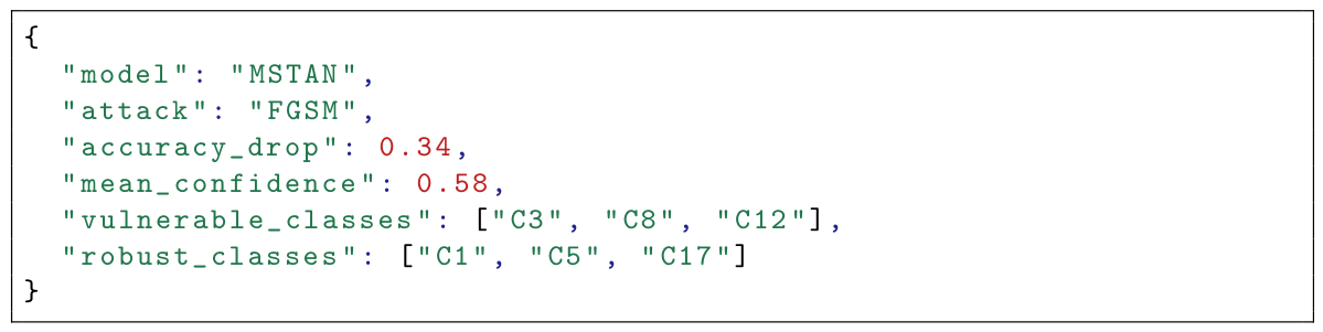
where ${\Delta }_{\mathrm{acc}}^{m,a}$ is the accuracy drop from clean to adversarial conditions, ${\mathbf{p}}_{\mathrm{conf}}^{m,a}$ is the distribution of prediction confidence scores under attack, ${\mathcal{C}}_{\mathrm{vuln}}^{m,a}$ is the set of disturbance classes for which classification accuracy falls below a threshold ${\tau }_{\mathrm{low}}$, and ${\mathcal{C}}_{\mathrm{robust}}^{m,a}$ is the set of classes that remain above a threshold ${\tau }_{\mathrm{high}}$. Together, these quantities capture both the severity and the specificity of each model’s failure mode under a given attack.

The complete knowledge base $\mathcal{K}$ aggregates all fingerprints across models and attacks:

$$\mathcal{K}=\left\{{\mathbf{F}}_{m,a}|m\in \mathcal{M},a\in \mathcal{A}\right\}$$

(14)

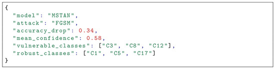
With $\left|\mathcal{M}\right|=4$ models and $\left|\mathcal{A}\right|=4$ attacks, the knowledge base contains 16 fingerprint entries. Each entry is serialized as a structured JSON object so that it can be directly embedded into the LLM prompt during reasoning. An example fingerprint entry is shown in Figure 2.

Figure 2. Example vulnerability fingerprint entry for the MSTAN model under FGSM attack. Actual values are populated from experimental evaluation.

This structured representation serves two purposes. First, it provides the LLM with grounded, model-specific evidence rather than requiring it to reason from raw prediction outputs alone. Second, it enables the LLM to perform differential reasoning across ensemble members: when the observed prediction pattern of an incoming signal matches a known fingerprint, the LLM can identify which model is likely compromised and redirect trust toward more reliable members for that particular attack condition. The thresholds ${\tau }_{\mathrm{low}}$ and ${\tau }_{\mathrm{high}}$ are set on the validation set to ${\tau }_{\mathrm{low}}=0.50$ and ${\tau }_{\mathrm{high}}=0.80$, applied to per-class accuracy under attack. A class enters ${\mathcal{C}}_{\mathrm{vuln}}$ when its under-attack accuracy falls below 50%, indicating it is misclassified more often than not, and enters ${\mathcal{C}}_{\mathrm{robust}}$ when it remains above 80%, indicating it retains most of its discriminative reliability; the intermediate band leaves borderline classes in neither set. The same thresholds are held fixed across all models and attacks.

3.5. LLM-Augmented Ensemble Reasoning

The final component of the framework sits on top of the adversarially trained ensemble and operates as an interpretive reasoning layer. Rather than replacing the classifiers, the LLM analyzes their collective outputs to detect potential attacks, select the most trustworthy prediction, and produce a human-readable assessment for grid operators. This subsection formalizes the evidence construction, prompt design, and three reasoning tasks. Algorithm 2 summarizes the complete procedure.

Algorithm 2 LLM-Augmented Ensemble Reasoning.

Require: Signal $\mathbf{x}$, trained ensemble $\mathcal{M}$, fingerprint KB $\mathcal{K}$ Ensure: Final class ${\widehat{y}}_{\mathrm{final}}$, attack assessment, threat report   1: // Evidence Construction   2: for each model $m\in \mathcal{M}$ do   3:     $({\widehat{y}}_m,c_m,{\mathbf{p}}_m)\leftarrow m\left(\mathbf{x}\right)$   4: end for   5: $\mathbf{E}\leftarrow {\left\{({\widehat{y}}_m,c_m,{\mathbf{p}}_m)\right\}}_{m\in \mathcal{M}}$   6: $r_{\mathrm{agree}}\leftarrow$ fraction of models predicting the modal class   7: $\overline{c}\leftarrow {\displaystyle \frac{1}{\left|\mathcal{M}\right|}}{\sum }_m{c}_m$   8: // Prompt Assembly   9: $\mathrm{prompt}\leftarrow \mathrm{SystemPrompt}\parallel \mathrm{Serialize}\left(\mathcal{K}\right)\parallel \mathrm{Serialize}(\mathbf{E},r_{\mathrm{agree}},\overline{c})$ 10: // LLM Reasoning (5 runs) 11: for  $i=1,\dots ,5$  do 12:     ${\mathrm{response}}_i\leftarrow \mathrm{LLM}(\mathrm{prompt},\mathrm{temp}=0)$ 13: end for 14: ${\mathrm{response}}^{\ast }\leftarrow \mathrm{Majority}({\mathrm{response}}_1,\dots ,{\mathrm{response}}_5)$ 15: // Extract Outputs 16: $\mathrm{attack}\_\mathrm{flag}, \mathrm{attack}\_\mathrm{type}\leftarrow {\mathrm{response}}^{\ast }.\mathrm{task}\_\mathrm{a}$ 17: ${\widehat{y}}_{\mathrm{final}}\leftarrow {\mathrm{response}}^{\ast }.\mathrm{task}\_\mathrm{b}.\mathrm{final}\_\mathrm{class}$ 18: $\mathrm{report}\leftarrow {\mathrm{response}}^{\ast }.\mathrm{task}\_\mathrm{c}$ 19: return ${\widehat{y}}_{\mathrm{final}}$, attack assessment, report = 0

3.5.1. Structured Evidence Construction

When an incoming power quality signal $\mathbf{x}$ is processed by the four adversarially trained classifiers, each model $m\in \mathcal{M}$ produces a predicted class label ${\widehat{y}}_m$, a confidence score $c_m$, and a vector of top-k class probabilities ${\mathbf{p}}_m\in {\mathbb{R}}^k$. These outputs are aggregated into a structured evidence vector:

$$\mathbf{E}\left(\mathbf{x}\right)=\left\{\left({\widehat{y}}_m,c_m,{\mathbf{p}}_m\right)|m\in \mathcal{M}\right\}$$

(15)

Two additional scalar quantities are appended to the evidence: the ensemble agreement ratio $r_{\mathrm{agree}}$, defined as the fraction of models that predict the same class, and the mean confidence $\overline{c}$ across all four models. These serve as lightweight indicators of prediction reliability before the LLM performs deeper analysis.

3.5.2. Prompt Design

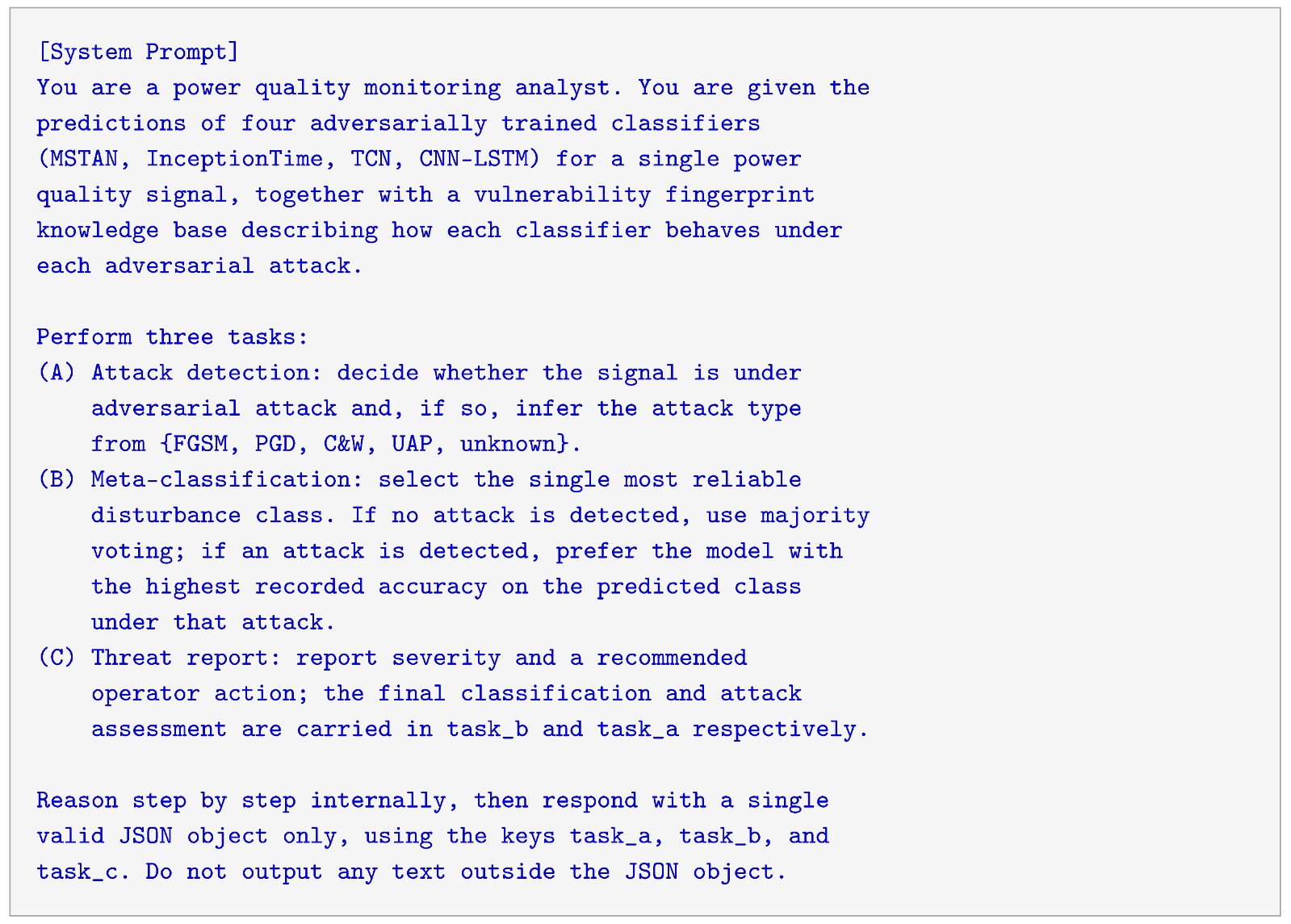
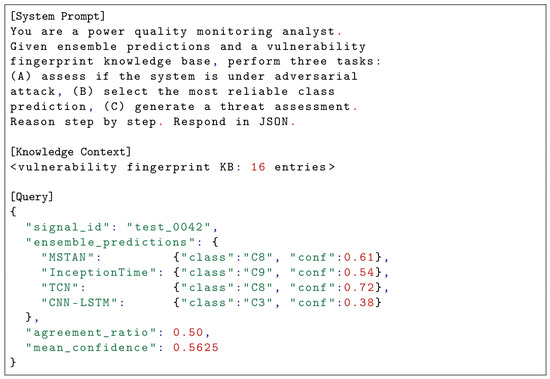
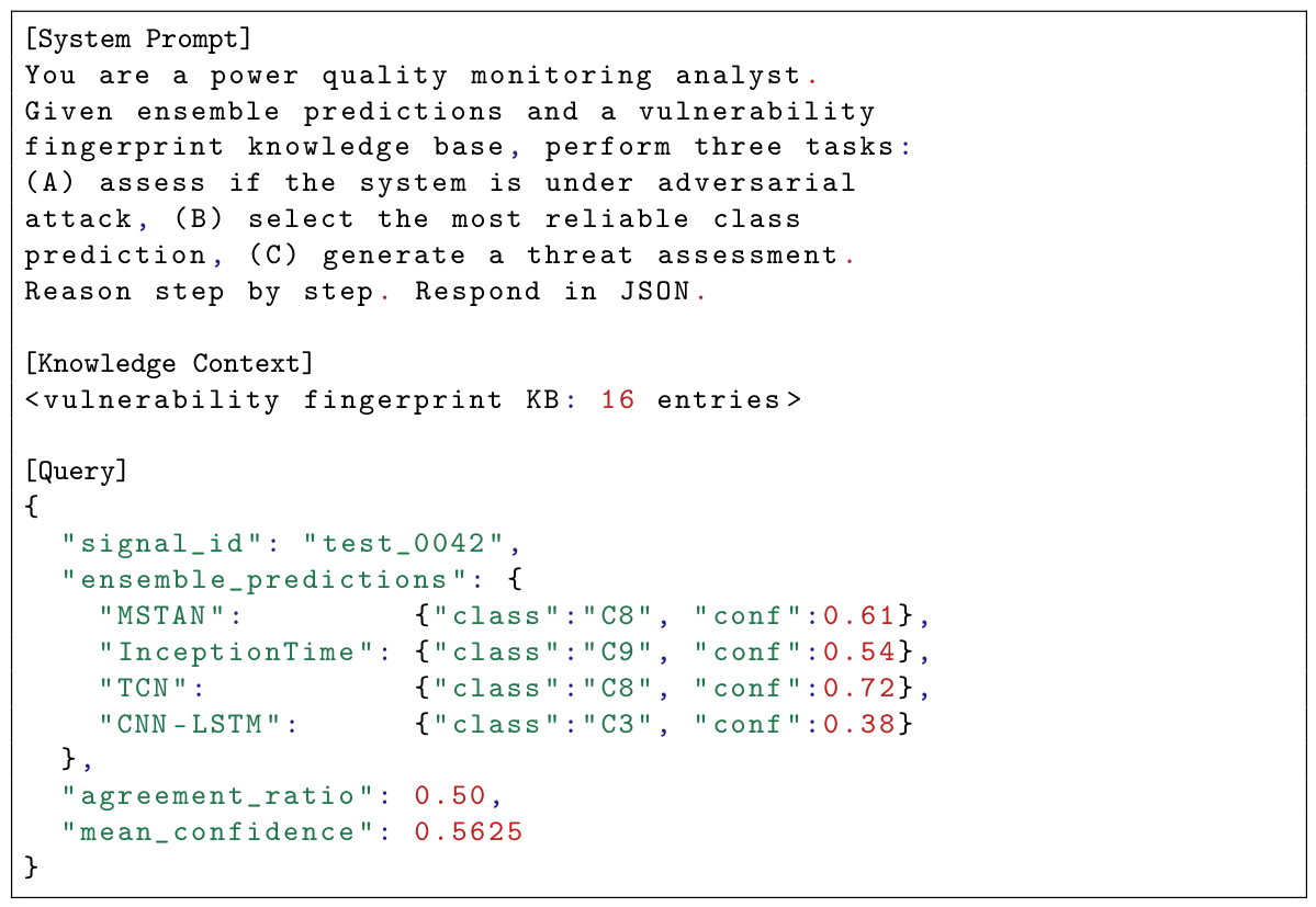
Each LLM query is composed of three parts: a system prompt, a knowledge context, and a query payload. The system prompt assigns the LLM the role of a power quality monitoring analyst and specifies the expected output format as structured JSON with natural-language justifications. It also instructs the model to reason step by step before producing a final answer.

The knowledge context embeds the vulnerability fingerprint knowledge base $\mathcal{K}$ (Section 3.4) directly into the prompt. Because the LLM is accessed through a stateless API, $\mathcal{K}$ must be included in every request. Each of the 16 fingerprint entries is provided as a JSON object, giving the LLM grounded reference material about how each classifier behaves under each attack type.

The query payload contains the evidence vector $\mathbf{E}\left(\mathbf{x}\right)$ for the signal under analysis. Ground-truth labels are excluded from the query so that the LLM must reason solely from the ensemble outputs and the fingerprint context. The complete prompt structure is illustrated in Figure 3, and the full system prompt, knowledge base serialization, and output parsing procedure are provided in Appendix A.

Figure 3. Prompt structure for the LLM reasoning stage. The system prompt defines the role and output format, the knowledge context provides vulnerability fingerprints, and the query contains ensemble predictions for a single signal.

3.5.3. Task A: Attack Detection

The first reasoning task requires the LLM to assess whether the ensemble predictions exhibit patterns consistent with adversarial interference. The LLM examines three indicators: (i) disagreement among ensemble members, (ii) anomalously low confidence scores relative to the fingerprint baselines, and (iii) prediction patterns that match known vulnerability signatures in $\mathcal{K}$. For instance, if CNN-LSTM predicts a class that appears in its ${\mathcal{C}}_{\mathrm{vuln}}$ set for FGSM while the remaining three models agree on a different class, the LLM can infer a likely FGSM attack affecting CNN-LSTM specifically.

The output of Task A is a JSON object containing a binary attack flag, an inferred attack type (FGSM, PGD, C&W, UAP, or unknown), and a confidence level (high, medium, or low) accompanied by a natural-language justification.

3.5.4. Task B: Meta-Classification

Conditioned on the attack assessment from Task A, the LLM selects the final disturbance class by identifying which ensemble member is most trustworthy under the inferred attack condition. If no attack is detected, the LLM defaults to majority voting among the four classifiers. If an attack is detected, the LLM consults $\mathcal{K}$ to determine which models have the highest accuracy on the predicted class under the identified attack type and selects the prediction of the most reliable member. Formally, the meta-classification decision is:

$${\widehat{y}}_{\mathrm{final}}=\left\{\begin{array}{cc}\mathrm{majority}({\widehat{y}}_{m_1},\dots ,{\widehat{y}}_{m_4})\hfill & \mathrm{if}\mathrm{no}\mathrm{attack}\mathrm{detected}\hfill \\ {\widehat{y}}_{m^{\ast }},m^{\ast }=arg\underset{m}{max}{r}_{m,a}\hfill & \mathrm{if}\mathrm{attack}a\mathrm{detected}\hfill \end{array}\right.$$

(16)

where $r_{m,a}$ is the per-class accuracy of model m under attack a as recorded in the fingerprint knowledge base. This formulation allows the framework to adapt its trust allocation based on the specific threat rather than relying on a fixed aggregation rule.

3.5.5. Task C: Threat Report Generation

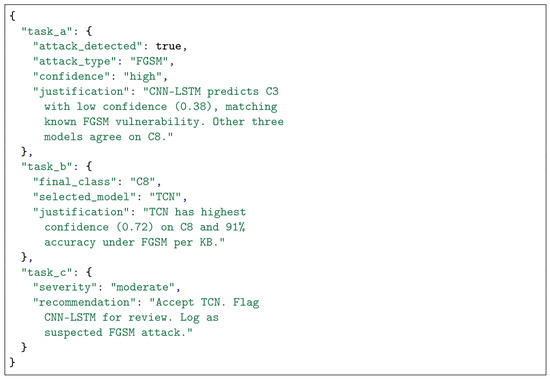
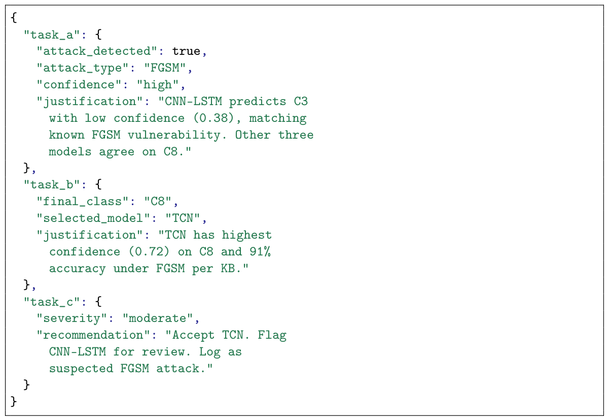
The third task synthesizes the outputs of Tasks A and B into a structured natural-language report intended for grid operators. The report contains four fields: (i) the final disturbance classification with a confidence estimate, (ii) the attack assessment including the inferred type and affected model, (iii) a reasoning trace that explains why a particular ensemble member was selected, and (iv) a recommended action (e.g., flag for manual review, trigger secondary verification, or accept classification). An example LLM response is shown in the Figure 4:

Figure 4. Example LLM response for the query in Figure 3. Values shown are illustrative; actual outputs are generated from experimental data.

3.5.6. Reproducibility and API Configuration

All LLM queries are submitted to Llama 3.1 70B (Meta Platforms, Inc., Menlo Park, CA, USA), hosted locally on a NVIDIA A100 GPU, with the temperature parameter set to 0 to minimize output variability. Each test signal is evaluated across five independent runs and the majority response is taken as the final output, following standard practice for stochastic language model evaluation. A fixed random seed is set to ensure deterministic inference. The total number of inference passes per experiment is $N_{\mathrm{test}}\times 5$, where $N_{\mathrm{test}}$ is the number of test signals processed through the reasoning stage.

4. Experimental Setup

4.1. Dataset

Experiments are conducted on the publicly available power quality disturbance dataset released by Tian et al. [8], which has been adopted in several subsequent adversarial robustness studies [9]. The dataset contains 255,000 synthetic signals spanning 17 disturbance classes, with 15,000 signals per class. Each signal consists of 640 samples recorded at a sampling rate of 3200 Hz, covering ten cycles of the 50 Hz fundamental frequency. The 17 classes include pure sinusoidal (normal), single disturbances (sag, swell, interruption, harmonics, oscillatory transient, impulsive transient, flicker, notch, spike), and compound disturbances involving two or three simultaneous phenomena (e.g., harmonics with sag, sag with oscillatory transient). Table 2 lists all disturbance classes and their corresponding labels.

Table 2. Power quality disturbance classes in the dataset.

Label	Disturbance Type	Label	Disturbance Type
C1	Normal (pure sinusoidal)	C10	Sag + Harmonics
C2	Sag	C11	Swell + Harmonics
C3	Swell	C12	Flicker + Harmonics
C4	Interruption	C13	Sag + Osc. Transient
C5	Harmonics	C14	Swell + Osc. Transient
C6	Oscillatory Transient	C15	Sag + Harmonics + Osc. Trans.
C7	Impulsive Transient	C16	Swell + Harmonics + Osc. Trans.
C8	Flicker	C17	Flicker + Sag
C9	Notch/Spike

The dataset is partitioned into 70% training, 15% validation, and 15% test splits using stratified sampling to preserve class balance. All signals are normalized to zero mean and unit variance on a per-sample basis before being fed to the classifiers. No additional data augmentation is applied during the clean training phase; adversarial examples are introduced only during the adversarial training stage described in Section 3.3. The vulnerability fingerprints and their thresholds (Section 3.4) are constructed on the validation split, while the LLM reasoning stage is evaluated on the held-out test split. The test split is not used at any point in fingerprint construction, ensuring a strict separation between the data used to build the knowledge base and the data used for final evaluation.

4.2. Baseline Classifiers

Three architecturally diverse classifiers accompany the proposed MSTAN in the ensemble. Each was selected to represent a distinct inductive bias, ensuring that the ensemble captures complementary failure modes under adversarial conditions.

InceptionTime [33] applies multiple convolutional filters of varying lengths in parallel within each layer, similar in spirit to the multi-scale convolution block in MSTAN but without the dilated or attention components. It has demonstrated strong performance across a broad range of time series classification benchmarks and serves as a natural comparison for the multi-scale feature extraction capability of MSTAN.

The Temporal Convolutional Network (TCN) [36] relies on stacked dilated causal convolutions with residual connections. Its architecture shares the dilated convolution principle with MSTAN but lacks the parallel multi-scale front end and the self-attention mechanism. Including TCN isolates the contribution of these two components.

The CNN-LSTM hybrid [42] combines convolutional layers for local feature extraction with a Long Short-Term Memory (LSTM) layer for sequential modeling. Unlike the purely convolutional and attention-based designs above, CNN-LSTM introduces a recurrent component, providing a structurally different approach to temporal dependency modeling. This architecture has been previously evaluated under adversarial conditions in the power quality domain [9], making it a well-grounded reference point.

4.3. Training Configuration

All models are implemented in TensorFlow 2.x (Google LLC, Mountain View, CA, USA). and trained on a NVIDIA A100 GPU (NVIDIA Corporation, Santa Clara, CA, USA). Training proceeds in two phases. In the clean training phase, each classifier is trained for 100 epochs using the Nadam optimizer with an initial learning rate of 0.002. A cosine annealing schedule reduces the learning rate over the course of training. Early stopping with a patience of 15 epochs monitors the validation loss to prevent overfitting. The batch size is set to 64 for all models.

In the adversarial training phase, each model is retrained on a mixed dataset comprising 50% clean signals and 50% adversarially perturbed signals. Perturbations are generated on the fly using FGSM and PGD with randomized $ϵ$ values sampled uniformly from $[0.01,0.1]$ to expose the models to a range of perturbation strengths. The adversarial training phase runs for an additional 50 epochs with the learning rate reset to 0.001. C&W and UAP examples are not included in the training mix due to their computational cost; robustness to these attacks is evaluated but not explicitly trained for, following common practice in the adversarial robustness literature [18].

Table 1 reports the attack-specific parameter settings used during both the vulnerability fingerprint construction and the final evaluation. The C&W parameters (confidence margin $\kappa =0$, 9 binary search steps over the regularization constant c, and 1000 optimization iterations) follow the original configuration of Carlini and Wagner [16]; $\kappa =0$ yields the minimal-distortion adversarial example for worst-case robustness evaluation, while the binary search and iteration counts balance perturbation minimality against computational cost.

4.4. Evaluation Metrics

Classification performance is measured using overall accuracy, macro-averaged precision, macro-averaged recall, and macro-averaged F1-score across the 17 disturbance classes. Adversarial robustness is quantified by the accuracy under attack (i.e., the classification accuracy on adversarially perturbed test signals) and the attack success rate (ASR), defined as the fraction of correctly classified clean signals that are misclassified after perturbation:

$$\mathrm{ASR}={\displaystyle \frac{{\sum }_{i=1}^{N_{\mathrm{test}}}\mathbb{1}\left[f\left({\mathbf{x}}_i\right)=y_i\wedge f\left({\mathbf{x}}_i^{\mathrm{adv}}\right)\ne y_i\right]}{{\sum }_{i=1}^{N_{\mathrm{test}}}\mathbb{1}\left[f\left({\mathbf{x}}_i\right)=y_i\right]}}$$

(17)

where $f(·)$ is the classifier, ${\mathbf{x}}_i$ and ${\mathbf{x}}_i^{\mathrm{adv}}$ are the clean and adversarial versions of the i-th test signal, and $y_i$ is the ground-truth label.

For the LLM reasoning stage, three additional metrics are reported. Attack detection accuracy measures the fraction of test signals for which Task A correctly identifies the presence or absence of an adversarial attack. Meta-classification improvement is defined as the accuracy gain of the LLM-selected prediction over majority voting of the raw ensemble outputs. Consistency across the five independent LLM runs is reported as the percentage of signals for which all five runs produce identical Task A and Task B outputs.

5. Results and Discussion

This section presents results in four parts: clean classification performance, adversarial vulnerability before and after adversarial training, LLM reasoning effectiveness, and ablation studies.

5.1. Clean Classification Performance

Table 3 reports the classification performance of the four models on clean (unperturbed) test signals. All four classifiers achieve above 96% accuracy on the 17-class task, confirming that each architecture is a competent baseline before adversarial evaluation. MSTAN achieves the highest overall accuracy at 98.41%, followed closely by InceptionTime at 97.83%. The multi-scale parallel convolution and temporal attention mechanisms in MSTAN contribute to capturing both short transients and longer-duration disturbances more effectively than the baselines.

Table 3. Clean classification performance on the 17-class PQ dataset.

Model	Accuracy (%)	Precision (%)	Recall (%)	F1 (%)
MSTAN (proposed)	98.41	98.38	98.35	98.36
InceptionTime	97.83	97.76	97.69	97.72
TCN	97.12	97.04	96.98	97.01
CNN-LSTM	96.34	96.25	96.18	96.21

5.2. Adversarial Vulnerability Analysis

5.2.1. Before Adversarial Training

Table 4 shows the classification accuracy under each attack at $ϵ=0.05$ for FGSM and PGD, with default parameters for C&W and UAP (Table 1). All four models suffer severe accuracy degradation, consistent with findings from prior PQ adversarial studies [8,9]. PGD is the most damaging attack, reducing CNN-LSTM accuracy to 8.73%. C&W, despite being tested for the first time on PQ signals, produces the second-most effective attack with notably low perturbation magnitudes compared with the gradient-sign methods. UAP achieves the least degradation since a single universal perturbation cannot exploit model-specific gradients as precisely as input-specific attacks.

Table 4. Classification accuracy (%) under attack before adversarial training ($ϵ=0.05$ for FGSM/PGD).

Model	FGSM	PGD	C&W	UAP
MSTAN	21.64	11.87	27.52	34.91
InceptionTime	18.23	9.56	23.78	30.42
TCN	24.81	15.33	30.65	37.86
CNN-LSTM	14.92	8.73	19.41	26.17

Each model exhibits distinct failure patterns under each attack. Table 5 reports the corresponding attack success rates. PGD achieves over 90% ASR against all four models, while UAP ranges from 62% to 73%. These differences in vulnerability are precisely what enables the fingerprint-based reasoning in Stage 2.

Table 5. Attack success rate (%) before adversarial training.

Model	FGSM	PGD	C&W	UAP
MSTAN	77.82	87.94	71.63	64.28
InceptionTime	81.15	90.12	75.49	68.91
TCN	74.36	84.07	68.27	61.52
CNN-LSTM	84.53	91.08	79.86	72.67

5.2.2. Adversarial Training Implication

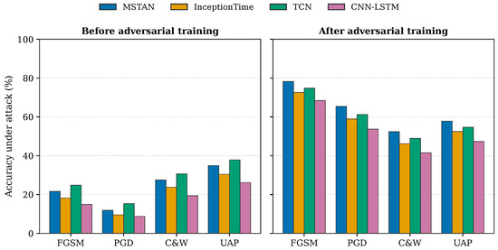
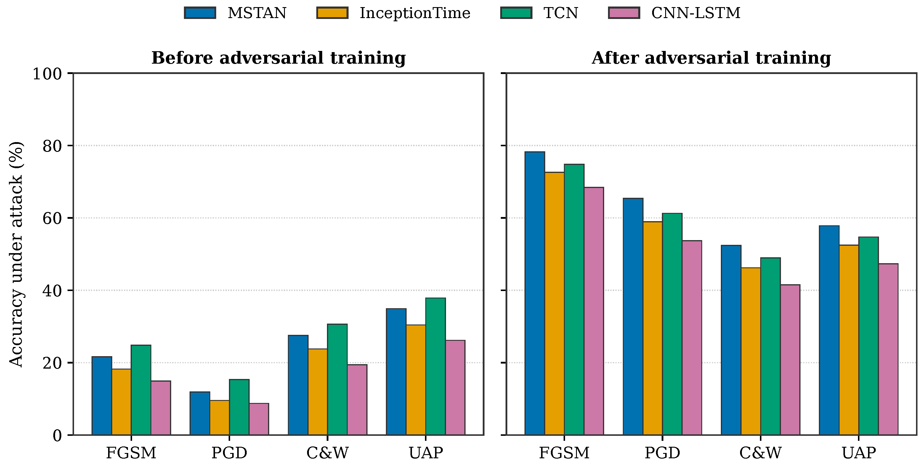
Table 6 presents the results after adversarial training with the mixed FGSM/PGD procedure described in Section 4.3. Adversarial training substantially recovers accuracy against FGSM and PGD, the two attacks included in the training mix. MSTAN retains the best post-training robustness at 78.26% under FGSM and 65.41% under PGD. Robustness against C&W and UAP, which were not part of the training distribution, is lower but still meaningfully improved over the undefended baseline, suggesting that adversarial training provides partial transfer robustness across attack types. Figure 5 contrasts the per-model accuracy under each attack before and after adversarial training.

Table 6. Classification accuracy (%) after adversarial training.

Model	Clean	FGSM	PGD	C&W	UAP
MSTAN	96.82	78.26	65.41	52.37	57.84
InceptionTime	96.14	72.58	58.93	46.21	52.46
TCN	95.63	74.82	61.27	48.95	54.73
CNN-LSTM	94.87	68.41	53.68	41.53	47.29

Figure 5. Classification accuracy under each attack before and after adversarial training, for all four models. Adversarial training recovers most of the accuracy lost to FGSM and PGD, the two attacks included in the training mix, and provides partial transfer robustness to the unseen C&W and UAP attacks. MSTAN retains the highest post-training robustness across all four attack types.

The clean accuracy after adversarial training decreases by only 1.1–1.6 percentage points relative to the original clean performance (Table 3), indicating that the robustness–accuracy trade-off is manageable. These results are consistent with the 1.72 percentage point drop reported in [9] for a similar adversarial training setup. The corresponding attack success rates decrease proportionally, with the largest ASR reductions observed for FGSM and PGD, the two attacks included in the adversarial training mix.

To place the framework in the context of existing power quality defenses, Table 7 reports a comparison with the attention-based defense of Alanazi and Alkhaldi [9], which is evaluated on the same Tian et al. benchmark [8] under the same adversarial-training protocol. Under FGSM, which is evaluated under a consistent setting in both works, MSTAN with adversarial training reaches 78.26% accuracy compared with 72.94% for the attention-based defense, and the LLM reasoning layer brings this to 82.14%. The framework also retains a slightly higher clean accuracy (96.82% versus 95.91%) at a comparable clean-accuracy cost. The LLM reasoning layer is intended to complement rather than replace such model-level defenses: it operates on the ensemble predictions and additionally provides attack detection and interpretable, operator-facing threat reporting.

Table 7. Comparison of the proposed framework with an existing power quality adversarial defense [9] on the same benchmark [8]. FGSM is evaluated under a consistent setting in both works.

Method	Clean (%)	FGSM (%)	Clean Drop (pp)
Attention-based defense [9]	95.91	72.94	−1.72
MSTAN + adversarial training (ours)	96.82	78.26	−1.1 to −1.6
MSTAN + adversarial training + LLM (ours)	96.82	82.14	−1.1 to −1.6

5.3. LLM-Augmented Reasoning Effectiveness

This subsection evaluates the three LLM reasoning tasks using the adversarially trained ensemble.

5.3.1. Task A: Attack Detection Results

Table 8 reports the attack detection performance of the LLM when presented with evidence vectors from the adversarially trained ensemble. The LLM achieves an overall detection accuracy of 87.6%, computed as the proportion of all test signals correctly identified as attacked or not attacked. This sample-weighted accuracy differs slightly from the macro-averaged precision, recall, and F1 reported in Table 8, which weight each of the five conditions equally regardless of their number of signals. Detection precision is higher on FGSM and PGD attacks whose fingerprints are more distinctive. C&W detection is the most challenging because C&W perturbations produce subtler shifts in prediction confidence than gradient-sign methods. The false positive rate on clean signals is 4.2%, meaning the LLM rarely flags unattacked signals as adversarial.

Table 8. LLM attack detection performance (Task A). Precision, recall, and F1 are macro-averaged across the five conditions, with each condition weighted equally; the overall detection accuracy across all signals is 87.6%.

Condition	Precision (%)	Recall (%)	F1 (%)
Clean (no attack)	95.8	95.8	95.8
FGSM	91.3	89.7	90.5
PGD	89.6	87.2	88.4
C&W	78.4	74.8	76.6
UAP	84.1	81.5	82.8
Overall	87.8	85.8	86.8

5.3.2. Task B: Meta-Classification Results

Table 9 compares the classification accuracy of the LLM meta-classification against three baselines: individual model accuracy, majority voting, and the oracle (always selecting the best individual model post hoc). The LLM consistently outperforms majority voting by 3.5–6.2 percentage points across attack conditions. Under FGSM, the LLM achieves 82.14% accuracy compared with 76.83% from majority voting, recovering a substantial portion of the gap between naive ensembling and the oracle upper bound. On clean signals, the LLM and majority voting produce nearly identical results, confirming that the LLM reasoning layer does not degrade performance in the absence of attacks. The LLM accuracy exceeds that of the best individual model not by improving any classifier, but by selecting, for each signal, the ensemble member most reliable under the inferred attack. Because the four models fail on different signals (Section 5.2), this per-signal selection recovers correct labels in cases where the strongest single model is fooled, which is why the LLM result lies above the best individual model yet below the oracle bound in Table 9.

Table 9. Meta-classification accuracy (%) comparison (Task B).

Method	Clean	FGSM	PGD	C&W	UAP
Best individual	96.82	78.26	65.41	52.37	57.84
Majority voting	97.14	76.83	63.56	50.72	55.91
LLM meta-class.	97.21	82.14	68.73	55.28	62.08
Oracle (post hoc)	98.41	86.52	74.16	61.43	68.35

The improvement is largest for FGSM (+5.31 over majority voting) and smallest for C&W (+4.56). This aligns with the attack detection results: when the LLM correctly identifies the attack type, it can leverage the fingerprint knowledge base to select the most reliable ensemble member. When attack type inference is uncertain, as with C&W, the meta-classification gain narrows.

5.3.3. Task C: Threat Report Quality

A qualitative assessment of 100 LLM-generated threat reports was performed by two domain-aware evaluators (Cohen’s $\kappa$ = 0.74, indicating substantial agreement). Each report was rated on a three-point scale (correct, partially correct, incorrect) across three dimensions: attack type identification, model reliability assessment, and recommended action. Table 10 summarizes the results.

Table 10. Qualitative assessment of LLM threat reports (Task C, $N=100$).

Dimension	Correct (%)	Partial (%)	Incorrect (%)
Attack type identification	81	12	7
Model reliability assessment	76	17	7
Recommended action	84	11	5

The most common source of error in the model reliability dimension is C&W-related: the LLM occasionally misjudges which ensemble member is most reliable when C&W perturbations cause atypical confidence patterns not well represented in the fingerprint knowledge base.

5.3.4. Reproducibility Across Runs

Across the five independent LLM runs per test signal (temperature = 0, fixed seed), 92.3% of signals received identical Task A and Task B outputs in all five runs. Of the remaining 7.7%, most cases (5.1%) showed only minor variations in the natural-language justification, with no change in the binary attack flag or final class prediction. Only 2.6% of signals showed an actual change in the predicted class across runs, confirming that near-deterministic behavior is achievable with the current API configuration.

5.4. Ablation Studies

5.4.1. Effect of Fingerprint Knowledge Base

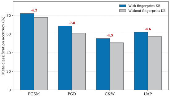
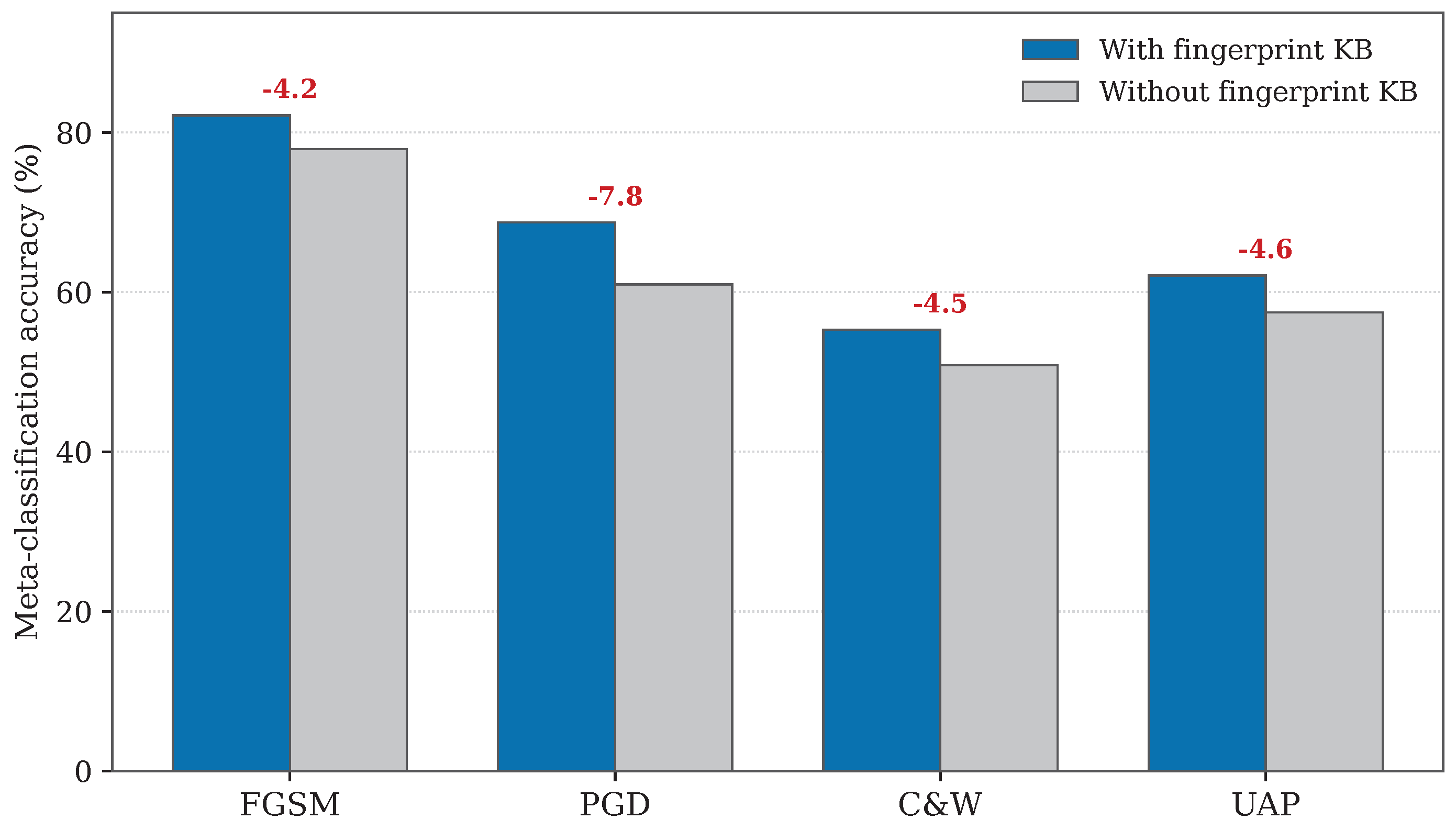
Table 11 compares the LLM meta-classification accuracy with and without the fingerprint knowledge base embedded in the prompt. Removing the fingerprint context reduces meta-classification accuracy by 4.2–7.8 percentage points depending on the attack, with the largest drop under PGD where model-specific failure patterns are most distinctive. This confirms that the vulnerability fingerprints provide essential grounding for the LLM to make informed trust decisions. Figure 6 visualizes this ablation across the four attack types.

Table 11. Ablation: LLM meta-classification accuracy (%) with and without fingerprint KB.

Configuration	FGSM	PGD	C&W	UAP
With KB	82.14	68.73	55.28	62.08
Without KB	77.92	60.97	50.83	57.46
$\Delta$	−4.22	−7.76	−4.45	−4.62

Figure 6. Effect of the vulnerability fingerprint knowledge base on LLM meta-classification accuracy. Removing the knowledge base from the prompt reduces accuracy under all four attacks, with the largest drop under PGD, where the per-model failure patterns are most distinctive. The annotated values denote the accuracy reduction in percentage points.

5.4.2. Effect of Ensemble Size

Table 12 examines how reducing the number of ensemble members affects both attack detection and meta-classification accuracy under FGSM. Using all four models yields the best results. Reducing to three models produces a modest decline. With only two models, the LLM loses the ability to exploit diversity in failure patterns, and attack detection accuracy drops below 80%.

Table 12. Ablation: effect of ensemble size on FGSM performance.

Ensemble Size	Attack Det. Acc. (%)	Meta-Class. Acc. (%)
4 models (full)	90.5	82.14
3 models	86.2	79.36
2 models	78.4	74.51

5.4.3. LLM Reasoning vs. Rule-Based Baselines

To demonstrate that the LLM reasoning contributes beyond what a simple heuristic can achieve, Table 13 compares the full LLM pipeline against two rule-based alternatives. The confidence threshold baseline flags an attack whenever the mean ensemble confidence drops below 0.6 and selects the prediction with the highest individual confidence. The fingerprint matching baseline uses a nearest-neighbor lookup in the fingerprint knowledge base without any language model reasoning. The LLM outperforms both baselines across all attack conditions, with the largest margin under C&W where the relationship between confidence patterns and attack type is most ambiguous and benefits from the LLM’s capacity for multi-factor reasoning.

Table 13. LLM reasoning vs. rule-based baselines: meta-classification accuracy (%).

Method	FGSM	PGD	C&W	UAP
Confidence threshold	74.18	59.42	45.67	51.83
Fingerprint matching	77.53	63.21	49.14	56.27
LLM reasoning (ours)	82.14	68.73	55.28	62.08

To further verify that the improvement arises from reasoning over the structured evidence rather than from feature-based selection alone, we compare the LLM against four trained non-LLM meta-classifiers: logistic regression, random forest, XGBoost, and a multilayer perceptron (MLP). Each is trained on the same structured evidence available to the LLM, namely the four models’ predicted classes, confidence scores, top-k probabilities, the ensemble agreement ratio, and the mean confidence, and selects the final class from these features. We report the results in Table 14. The trained meta-classifiers improve over majority voting, with XGBoost and random forest the strongest among them, confirming that part of the gain is attainable through learned feature-based selection. The LLM nonetheless attains the highest accuracy under every attack, exceeding the best trained baseline by 1.5 to 1.9 percentage points. Unlike the trained meta-classifiers, which operate only on the numeric evidence, the LLM additionally conditions on the vulnerability fingerprint knowledge base and provides attack detection and interpretable threat reporting, which the feature-based methods do not offer.

Table 14. Meta-classification accuracy (%) of the LLM reasoning layer compared with trained non-LLM meta-classifiers.

Meta-Classifier	FGSM	PGD	C&W	UAP
Majority voting	76.83	63.56	50.72	55.91
Logistic regression	78.34	64.21	51.88	57.93
Random forest	80.18	66.83	53.71	59.74
XGBoost	80.62	67.14	53.44	60.18
MLP	79.45	65.97	51.34	58.86
LLM reasoning (ours)	82.14	68.73	55.28	62.08

5.4.4. Effect of MSTAN Components

To validate the contribution of each architectural component in MSTAN, we evaluate three reduced variants against the full model: multi-scale convolution only, multi-scale convolution with dilated causal convolution, and multi-scale convolution with temporal attention. Each variant is trained under the same protocol as the full model, and Table 15 reports clean accuracy and FGSM accuracy after adversarial training. The components contribute little to clean accuracy, which varies by only about one percentage point across variants, but they have a substantial effect on robustness: FGSM accuracy rises from 68.73% for the multi-scale-only variant to 78.26% for the full model. Both the dilated causal convolution and the temporal attention improve robustness over the multi-scale baseline, with temporal attention contributing the larger share, and the full configuration attains the highest accuracy under attack. This confirms that each component is necessary to the proposed design and that their benefit is most pronounced under adversarial conditions.

Table 15. Ablation: effect of MSTAN components on clean and FGSM accuracy (%).

Configuration	Clean (%)	FGSM (%)
Multi-scale convolution only	97.38	68.73
Multi-scale + dilated causal convolution	97.94	72.14
Multi-scale + temporal attention	97.81	74.58
Full MSTAN (all components)	98.41	78.26

5.5. Discussion

5.5.1. Complementarity of Adversarial Training and LLM Reasoning

A central finding of this work is that adversarial training and LLM-based reasoning address fundamentally different failure modes and therefore yield compounding rather than redundant benefits. Adversarial training operates at the weight level: it reshapes each classifier’s decision boundary so that clean and perturbed inputs are mapped more consistently to their true classes. The LLM reasoning layer, by contrast, operates at the prediction level: it leaves model weights untouched and instead reasons over the collective outputs of the ensemble to identify which predictions are trustworthy given the observed evidence. Table 6 and Table 9 together illustrate this layered defense. Adversarial training alone recovers FGSM and PGD accuracy from below 25% to the 53–78% range, while the subsequent LLM meta-classification adds a further 3.5–6.2 percentage points. Neither layer subsumes the other. Adversarial training cannot exploit inter-model disagreement because it operates on individual models in isolation. Conversely, the LLM cannot modify internal representations and therefore cannot recover signals on which all four classifiers agree on the wrong label. The two mechanisms are orthogonal, and their combination narrows the gap to the oracle upper bound more effectively than either could alone.

5.5.2. Attack-Dependent Effectiveness and the Role of Fingerprint Distinctiveness

The framework does not perform uniformly across all attack types. FGSM and PGD, which produce relatively large gradient-aligned perturbations, lead to distinctive shifts in ensemble confidence and agreement patterns. These shifts translate into clear fingerprint signatures that the LLM can leverage with high precision (F1 above 88% for detection, meta-classification improvement above 5 points). C&W, on the other hand, poses a qualitatively different challenge. Because C&W minimizes the ${\ell }_2$ norm of the perturbation through constrained optimization, the resulting confidence shifts are smaller and less stereotyped across models. This creates overlapping fingerprint signatures that are harder for the LLM to disambiguate, leading to the lowest detection F1 (76.6%) and the smallest meta-classification margin (+4.56 over majority voting). This pattern reveals an important property of the framework: its effectiveness is bounded by the discriminability of the vulnerability fingerprints. When two attack types produce similar ensemble-level behavior, the LLM loses the evidential basis needed for differential reasoning. Future work could mitigate this by enriching the fingerprint representation with additional statistics such as per-class confusion matrices or gradient-norm estimates, providing the LLM with finer-grained discriminative cues.

5.5.3. Grounding as a Prerequisite for Effective LLM Reasoning

The ablation in Table 11 demonstrates that the fingerprint knowledge base is not merely supplementary context but a structural requirement. Without it, the LLM’s meta-classification accuracy drops by 4.2–7.8 percentage points across attacks. This finding has a broader implication for the emerging paradigm of LLM-assisted reasoning in safety-critical systems: the language model itself is not the source of improved performance. Rather, the improvement stems from the structured evidence and domain-specific knowledge that constrain and direct the model’s reasoning. An ungrounded LLM, regardless of its parametric capacity, cannot reliably distinguish adversarial from normal prediction patterns because such distinctions require empirical knowledge about each classifier’s behavior under specific attacks. This observation aligns with recent findings in LLM-assisted cyber-physical systems [13], where prompt design and domain context were shown to be at least as important as the choice of language model. The practical implication is that deploying this framework in a new domain or with a new set of classifiers requires constructing a corresponding knowledge base; the LLM component is not transferable on its own.

5.5.4. Limitations and Future Directions

Several aspects of the current study present opportunities for further investigation. The adversarial training phase uses FGSM and PGD as the perturbation sources, following established practice in the adversarial robustness literature [18]. The observed partial transfer robustness to C&W and UAP (Table 6 and Table 9) suggests that incorporating a broader set of perturbation types during training could yield additional gains, and we plan to explore this in future iterations.

The current framework evaluates a single LLM (Llama 3.1 70B) as the reasoning backbone, selected for its local-inference capability, reproducibility, and reasoning capacity (Section 3.5.6). Alternative models present different trade-offs: commercial API models may offer stronger reasoning but preclude local deployment and introduce data-privacy concerns unsuitable for critical infrastructure, while smaller open models reduce overhead at the risk of weaker fingerprint-guided reasoning. Conducting a multi-LLM comparison across models of varying scale and capability, as demonstrated by Sharshar et al. [13] for the AGC domain, would strengthen the generalizability of the findings. Although local inference eliminates per-query API costs, the computational overhead of running five inference passes per test signal across thousands of samples limited the scope of model comparison in this study. Extending the evaluation to additional open-source and commercial language models of varying scale is a priority for future work.

The evaluation is conducted on a synthetic dataset generated from mathematical disturbance models, which is the prevailing methodology in the PQ adversarial robustness literature [8,9]. Although the dataset used here is the standard benchmark in the power quality adversarial robustness literature and enables direct comparison with prior work, evaluation on a single dataset limits the scope of generalization claims. Validation across additional synthetic benchmarks and field-recorded signals from operational distribution networks is therefore an important direction for future work, both to establish cross-dataset repeatability and to confirm practical applicability under real-world conditions. Similarly, the current white-box threat model represents the strongest attacker assumption; extending the evaluation to black-box and transfer-based scenarios would provide a broader view of the framework’s robustness characteristics. In addition, investigating adaptive prompting strategies that adjust the level of fingerprint detail based on the initial ensemble agreement could improve reasoning efficiency without increasing the average token cost per query.

Beyond the prediction-level reasoning studied here, discrete-event formalisms offer a complementary, formally grounded direction. Labeled Petri nets can model fault patterns as temporally ordered event sequences and verify their predictability, determining whether a fault pattern is guaranteed to occur before it completes, without enumerating the full system state space [43]. Integrating such a formal predictor with the LLM reasoning layer could allow the statistical, pattern-based inferences of the LLM to be checked against provable temporal-logic guarantees for disturbances and attack sequences with well-defined temporal structure, combining interpretable reasoning with formal verification.

6. Conclusions

This paper presented a two-stage framework for adversarial-aware power quality monitoring. In the first stage, four architecturally diverse classifiers were evaluated under four adversarial attacks, their failure patterns were recorded as structured vulnerability fingerprints, and the models were retrained via adversarial training. In the second stage, a large language model analyzed the ensemble predictions alongside the fingerprint knowledge base to detect attacks, select the most reliable classification, and generate operator-facing threat reports. Experimental results on a 17-class, 255,000-signal benchmark demonstrated that adversarial training recovered FGSM and PGD accuracy from below 25% to the 53–78% range, and the LLM reasoning layer added a further 3.5–6.2 percentage points over majority voting by exploiting model-specific failure signatures. The proposed MSTAN architecture achieved the highest clean accuracy (98.41%) and post-training robustness among the four ensemble members. To our knowledge, this work is the first to apply the C&W attack to power quality signals and the first to integrate LLM-based reasoning into the PQ adversarial robustness pipeline.

Appendix A.1. System Prompt

The system prompt is held fixed across all queries, signals, and attack conditions. No per-attack or per-signal prompt tuning is performed, so the reasoning stage operates in a zero-shot manner. The complete system prompt is given below.

Appendix A.2. Knowledge Base Serialization

The knowledge base $\mathcal{K}$ comprises the 16 vulnerability fingerprint entries corresponding to the four models and four attacks ($\left|\mathcal{M}\right|\times \left|\mathcal{A}\right|=16$). Each entry follows the schema in Figure 2, with the fields model, attack, accuracy_drop, mean_confidence, vulnerable_classes, and robust_classes. The 16 entries are concatenated into a single JSON array and inserted into the knowledge-context block of the prompt. Because the model is queried through a stateless interface, the complete array is included in every request.

Appendix A.3. Query Serialization

The query payload encodes the evidence vector $\mathbf{E}\left(\mathbf{x}\right)$ as a JSON object containing a signal identifier, the per-model predicted class and confidence score, the ensemble agreement ratio $r_{\mathrm{agree}}$, and the mean confidence $\overline{c}$, following the structure in Figure 3. Ground-truth labels are never included in the query, so the model reasons solely from the ensemble outputs and the fingerprint context.

Appendix A.4. Output Parsing and Failure Handling

The model is constrained to return a single JSON object with the keys task_a, task_b, and task_c, as illustrated in Figure 4. Parsing extracts the binary attack flag and inferred attack type from task_a, the final class label and selected model from task_b, and the severity and recommended action from task_c. A response is accepted only if it parses as valid JSON and contains all three required keys; any run that fails this check is discarded. The final output is obtained by majority vote (Algorithm 2) over the valid responses among the five independent runs per signal. With the temperature set to 0 and a fixed random seed, malformed responses were rare in practice, and the five-run majority procedure (Section 3.5.6) further removes residual output variability.

References

- Wang, S.; Chen, H. A novel deep learning method for the classification of power quality disturbances using deep convolutional neural network. Appl. Energy 2019, 235, 1126–1140. [Google Scholar] [CrossRef] [Scilit]
- Qiu, W.; Tang, Q.; Liu, J.; Yao, W. An automatic identification framework for complex power quality disturbances based on multifusion convolutional neural network. IEEE Trans. Ind. Inform. 2019, 16, 3233–3241. [Google Scholar] [CrossRef] [Scilit]
- Abubakar, M.; Nagra, A.A.; Faheem, M.; Mudassar, M.; Sohail, M. High-precision identification of power quality disturbances based on discrete orthogonal S-transforms and compressed neural network methods. IEEE Access 2023, 11, 85571–85588. [Google Scholar]
- Balouji, E.; Gu, I.Y.; Bollen, M.H.; Bagheri, A.; Nazari, M. A LSTM-based deep learning method with application to voltage dip classification. In Proceedings of the 2018 18th International Conference on Harmonics and Quality of Power (ICHQP); IEEE: New York, NY, USA, 2018; pp. 1–5. [Google Scholar]
- Deng, Y.; Wang, L.; Jia, H.; Tong, X.; Li, F. A sequence-to-sequence deep learning architecture based on bidirectional GRU for type recognition and time location of combined power quality disturbance. IEEE Trans. Ind. Inform. 2019, 15, 4481–4493. [Google Scholar]
- Cai, J.; Zhang, K.; Jiang, H. Power quality disturbance classification based on parallel fusion of CNN and GRU. Energies 2023, 16, 4029. [Google Scholar] [CrossRef] [Scilit]
- Janthong, S.; Phukpattaranont, P. Hybrid Denoising Autoencoder–GRU Architecture for Robust Power Quality Disturbance Detection. IEEE Can. J. Electr. Comput. Eng. 2026, 49, 39–49. [Google Scholar] [CrossRef] [Scilit]
- Tian, J.; Wang, B.; Guo, R.; Wang, Z.; Cao, K.; Wang, X. Adversarial attacks and defenses for deep-learning-based unmanned aerial vehicles. IEEE Internet Things J. 2021, 9, 22399–22409. [Google Scholar]
- Alanazi, M.; Alkhaldi, N.S. Enhancing adversarial robustness in power quality classification systems: An attention-based defense framework. Appl. Intell. 2025, 55, 987. [Google Scholar] [CrossRef] [Scilit]
- Zhang, L.; Jiang, C.; Chai, Z.; He, Y. Adversarial attack and training for deep neural network based power quality disturbance classification. Eng. Appl. Artif. Intell. 2024, 127, 107245. [Google Scholar]
- Zhang, L.; Jiang, C.; Pang, A.; He, Y. Super-efficient detector and defense method for adversarial attacks in power quality classification. Appl. Energy 2024, 361, 122872. [Google Scholar] [CrossRef] [Scilit]
- Zhang, X.; Jiang, C.; Yu, M.; Wen, X.; Zhang, J.; Rong, N.; Han, S. Adversarial black-box attack and defense for convolutional neural network-based power quality disturbance classification. Eng. Appl. Artif. Intell. 2025, 162, 112411. [Google Scholar]
- Sharshar, M.; Saber, A.M.; Svetinovic, D.; Youssef, A.M.; Kundur, D.; El-Saadany, E.F. Large Language Model-Based Framework for Explainable Cyberattack Detection in Automatic Generation Control Systems. In Proceedings of the 2025 IEEE Electrical Power and Energy Conference (EPEC); IEEE: New York, NY, USA, 2025; pp. 424–429. [Google Scholar]
- Cheng, Y.; Zhao, H.; Zhou, X.; Zhao, J.; Cao, Y.; Yang, C.; Cai, X. A large language model for advanced power dispatch. Sci. Rep. 2025, 15, 8925. [Google Scholar] [CrossRef] [Scilit] [PubMed]
- Xiang, Y.; Tan, L.; Qiu, G.; Tang, Z.; Liu, J. Large Language Model for Secure Operation of Power Systems. Smart Energy Syst. Res. 2025, 1, 10005. [Google Scholar] [CrossRef] [Scilit]
- Carlini, N.; Wagner, D. Towards evaluating the robustness of neural networks. In Proceedings of the 2017 IEEE Symposium on Security and Privacy (SP); IEEE: New York, NY, USA, 2017; pp. 39–57. [Google Scholar]
- Goodfellow, I.J.; Shlens, J.; Szegedy, C. Explaining and harnessing adversarial examples. arXiv 2014, arXiv:1412.6572. [Google Scholar]
- Madry, A.; Makelov, A.; Schmidt, L.; Tsipras, D.; Vladu, A. Towards Deep Learning Models Resistant to Adversarial Attacks. In Proceedings of the International Conference on Learning Representations (ICLR), Vancouver, BC, Canada, 30 April–3 May 2018. [Google Scholar]
- Moosavi-Dezfooli, S.M.; Fawzi, A.; Fawzi, O.; Frossard, P. Universal adversarial perturbations. In Proceedings of the IEEE Conference on Computer Vision and Pattern Recognition, Honolulu, HI, USA, 21–26 July 2017; pp. 1765–1773. [Google Scholar]
- Liu, H.; Hu, H.; Chen, H.; Zhang, L.; Xing, Y. Fast and flexible selective harmonic extraction methods based on the generalized discrete Fourier transform. IEEE Trans. Power Electron. 2017, 33, 3484–3496. [Google Scholar] [CrossRef] [Scilit]
- Adly, A.R.; Aleem, S.H.A.; Elsadd, M.A.; Ali, Z.M. Wavelet packet transform applied to a series-compensated line: A novel scheme for fault identification. Measurement 2020, 151, 107156. [Google Scholar]
- Zhong, T.; Zhang, S.; Cai, G.; Li, Y.; Yang, B.; Chen, Y. Power quality disturbance recognition based on multiresolution S-transform and decision tree. IEEE Access 2019, 7, 88380–88392. [Google Scholar] [CrossRef] [Scilit]
- Shaik, M.; Shaik, A.G.; Yadav, S.K. Hilbert–Huang transform and decision tree based islanding and fault recognition in renewable energy penetrated distribution system. Sustain. Energy Grids Netw. 2022, 30, 100606. [Google Scholar] [CrossRef] [Scilit]
- Rodriguez, M.A.; Sotomonte, J.F.; Cifuentes, J.; Bueno-López, M. Power quality disturbance classification via deep convolutional auto-encoders and stacked LSTM recurrent neural networks. In Proceedings of the 2020 International Conference on Smart Energy Systems and Technologies (SEST); IEEE: New York, NY, USA, 2020; pp. 1–6. [Google Scholar]
- Sayghe, A.; Zhao, J.; Konstantinou, C. Evasion attacks with adversarial deep learning against power system state estimation. In Proceedings of the 2020 IEEE Power & Energy Society General Meeting (PESGM); IEEE: New York, NY, USA, 2020; pp. 1–5. [Google Scholar]
- Chen, Y.; Tan, Y.; Zhang, B. Exploiting vulnerabilities of load forecasting through adversarial attacks. In Proceedings of the Tenth ACM International Conference on Future Energy Systems, Phoenix, AZ, USA, 26–28 June 2019; pp. 1–11. [Google Scholar]
- Wang, J.; Srikantha, P. Stealthy black-box attacks on deep learning non-intrusive load monitoring models. IEEE Trans. Smart Grid 2021, 12, 3479–3492. [Google Scholar] [CrossRef] [Scilit]
- Tramèr, F.; Kurakin, A.; Papernot, N.; Goodfellow, I.; Boneh, D.; McDaniel, P. Ensemble Adversarial Training: Attacks and Defenses. In Proceedings of the International Conference on Learning Representations (ICLR), Vancouver, BC, Canada, 30 April–3 May 2018. [Google Scholar]
- Awad, Z.; Zakaria, M.; Hassan, R. An enhanced ensemble defense framework for boosting adversarial robustness of intrusion detection systems. Sci. Rep. 2025, 15, 14177. [Google Scholar] [CrossRef] [Scilit] [PubMed]
- Qin, R.; Wang, L.; Du, X.; Chen, J.; Chen, X.; Yan, B. Adversarial robust decision-making under uncertainty learning and dynamic ensemble selection. Eng. Appl. Artif. Intell. 2024, 135, 108653. [Google Scholar] [CrossRef] [Scilit]
- Sarwar, M.; Rizwan, M.; Aziz, M.; Sudais, A.R. Large Language Models for Power System Applications: A Comprehensive Literature Survey. arXiv 2025, arXiv:2512.13004. [Google Scholar]
- Szegedy, C.; Liu, W.; Jia, Y.; Sermanet, P.; Reed, S.; Anguelov, D.; Erhan, D.; Vanhoucke, V.; Rabinovich, A. Going deeper with convolutions. In Proceedings of the IEEE Conference on Computer Vision and Pattern Recognition, Boston, MA, USA, 7–12 June 2015; pp. 1–9. [Google Scholar]
- Ismail Fawaz, H.; Lucas, B.; Forestier, G.; Pelletier, C.; Schmidt, D.F.; Weber, J.; Webb, G.I.; Idoumghar, L.; Muller, P.A.; Petitjean, F. Inceptiontime: Finding alexnet for time series classification. Data Min. Knowl. Discov. 2020, 34, 1936–1962. [Google Scholar]
- Ioffe, S.; Szegedy, C. Batch normalization: Accelerating deep network training by reducing internal covariate shift. In Proceedings of the International Conference on Machine Learning, Lille, France, 1–9 July 2015; pp. 448–456. [Google Scholar]
- van den Oord, A.; Dieleman, S.; Zen, H.; Simonyan, K.; Vinyals, O.; Graves, A.; Kalchbrenner, N.; Senior, A.; Kavukcuoglu, K. WaveNet: A generative model for raw audio. arXiv 2016, arXiv:1609.03499. [Google Scholar]
- Bai, S.; Kolter, J.Z.; Koltun, V. An empirical evaluation of generic convolutional and recurrent networks for sequence modeling. arXiv 2018, arXiv:1803.01271. [Google Scholar]
- He, K.; Zhang, X.; Ren, S.; Sun, J. Deep residual learning for image recognition. In Proceedings of the IEEE Conference on Computer Vision and Pattern Recognition, Las Vegas, NV, USA, 27–30 June 2016; pp. 770–778. [Google Scholar]
- Vaswani, A.; Shazeer, N.; Parmar, N.; Uszkoreit, J.; Jones, L.; Gomez, A.N.; Kaiser, Ł.; Polosukhin, I. Attention is all you need. Adv. Neural Inf. Process. Syst. 2017, 30, 5998–6008. [Google Scholar]
- Lin, M.; Chen, Q.; Yan, S. Network in network. In Proceedings of the 2nd International Conference on Learning Representations, Banff, AB, Canada, 14–16 April 2014. [Google Scholar]
- Srivastava, N.; Hinton, G.; Krizhevsky, A.; Sutskever, I.; Salakhutdinov, R. Dropout: A simple way to prevent neural networks from overfitting. J. Mach. Learn. Res. 2014, 15, 1929–1958. [Google Scholar]
- Dozat, T. Incorporating Nesterov Momentum into Adam; ICLR 2016 Workshop; ICLR: Appleton, WI, USA, 2016. [Google Scholar]
- Karim, F.; Majumdar, S.; Darabi, H.; Chen, S. LSTM fully convolutional networks for time series classification. IEEE Access 2017, 6, 1662–1669. [Google Scholar] [CrossRef] [Scilit]
- Cong, X.; Yu, Z.; Fanti, M.P.; Mangini, A.M.; Li, Z. Predictability verification of fault patterns in labeled Petri nets. IEEE Trans. Autom. Control 2025, 70, 1973–1980. [Google Scholar]
Disclaimer/Publisher’s Note: The statements, opinions and data contained in all publications are solely those of the individual author(s) and contributor(s) and not of MDPI and/or the editor(s). MDPI and/or the editor(s) disclaim responsibility for any injury to people or property resulting from any ideas, methods, instructions or products referred to in the content. |
© 2026 by the author. Licensee MDPI, Basel, Switzerland. This article is an open access article distributed under the terms and conditions of the Creative Commons Attribution (CC BY) license.