Fuzzy Inference System for Interpretable Classification of Wafer Map Defect Patterns

Abstract

Accurate classification of wafer map defect patterns is crucial for enhancing yield in semiconductor manufacturing. To address the problem of deep learning model over-fitting to label noise present in real industrial data, this study proposes a fuzzy logic-based framework for identifying both single and composite-type defect patterns. To demonstrate the robustness of our approach, we utilized the public dataset WM-811K and developed a Fuzzy Inference System (FIS) that leverages quantitative metrics such as the Center Zone Density (CZD). Data quality was also improved through preprocessing steps, including resolving class imbalances and refining labels via expert review. The performance of the proposed FIS was evaluated against a quantitative feature-based neural network, an FIS-neural network hybrid, and a CNN model. Experimental results showed that in single-pattern classification, the proposed FIS model achieved the highest accuracy of 99.20%, followed by the feature-based neural network (91.63%), the FIS-neural network hybrid model (88.55%), and the CNN (81.06%). These results prove that the proposed FIS approach maintains high classification accuracy while offering the advantages of interpretability and rule-based adjustability. This framework presents a practical solution that can effectively integrate domain knowledge to reduce the risk of overfitting in data environments with imperfect labels.

1. Introduction

In semiconductor manufacturing, rapidly and accurately classifying defect patterns on wafer maps is a core task for yield improvement and process stabilization. As integrated circuits become more highly integrated and wafer sizes continue to grow, ensuring interpretability of the results alongside automation of the classification process has emerged as an important technical challenge. The effective defect pattern recognition enables early detection of process anomalies and facilitates root-cause analysis, ultimately reducing production costs and enhancing device reliability.

A key stage for assessing final yield and stability in semiconductor manufacturing is the Electrical Die Sort (EDS) test. In this process, every individual die on a wafer undergoes electrical characterization to determine whether it operates normally. The test results are aggregated into a Wafer Bin Map (WBM), which visually indicates the pass/fail status of each die.

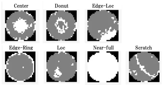
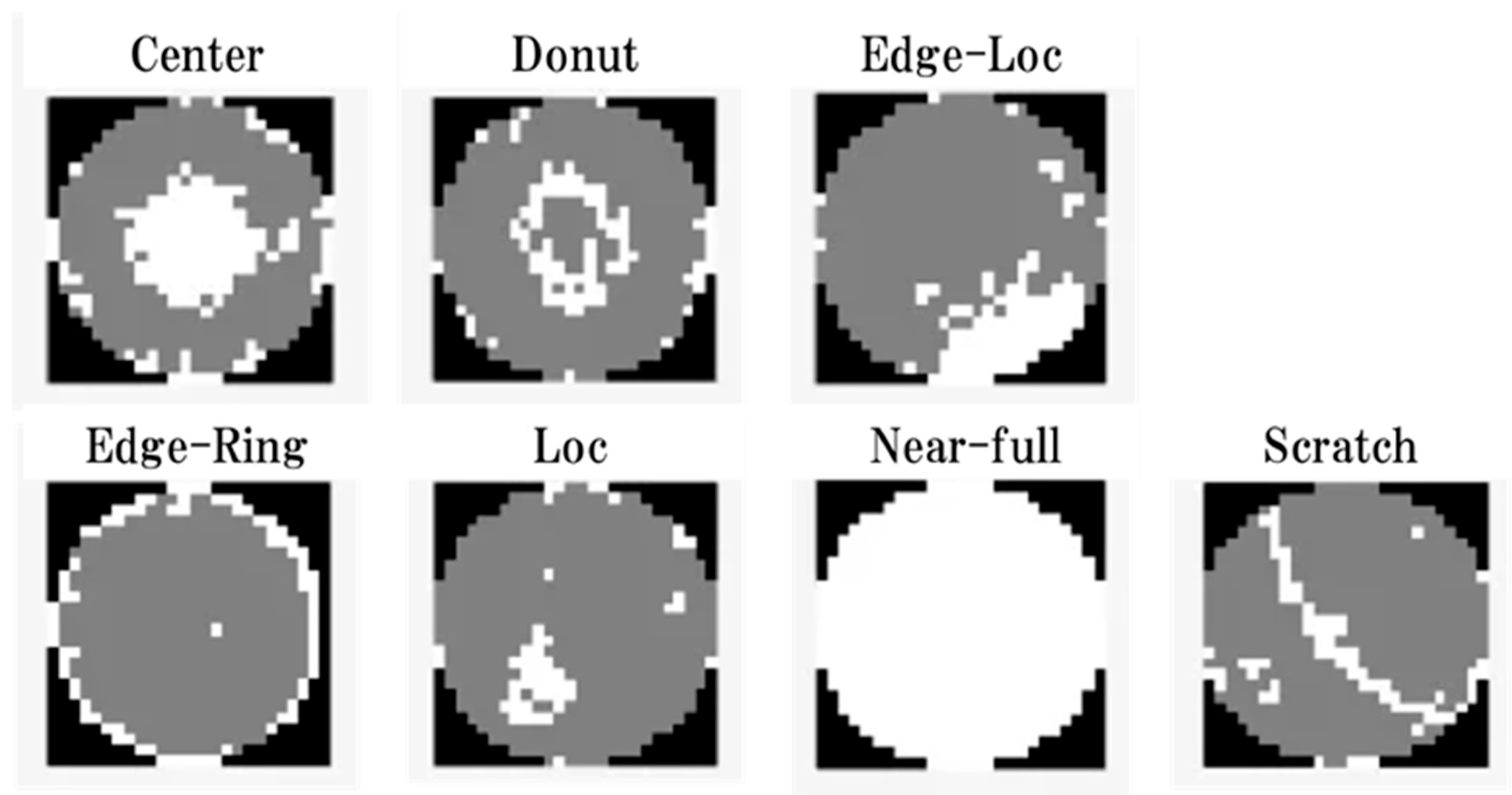
The spatial distribution of defective dies on this map often forms specific failure patterns. Figure 1 shows representative failure patterns observed in WBMs. White denotes defective chips, gray indicates good chips, and black represents the area outside the wafer map. “Center” refers to defects concentrated near the center of the wafer; “Donut” and “Edge-Ring” indicate ring-shaped defects appearing around the center and along the edge, respectively; “Loc” and “Edge-Loc” indicate localized defects near the center and near the edge, respectively; “Near-full” denotes that defects are densely populated across the entire wafer map; and “Scratch” refers to long, thin, line-shaped defect patterns. Each of these can be interpreted as a signal of anomalies at specific process stages. Therefore, rapid and accurate classification of such defect patterns is crucial for identifying root causes of yield degradation and stabilizing the process.

Figure 1. Examples of 26 × 26 WBM with labeling in WM-811K.

In research on wafer-map defect classification, the publicly available benchmark dataset WM-811K has been widely used [1,2,3,4,5]. However, this dataset contains class imbalance and substantial label noise, reflecting the complexity of real manufacturing environments. Although deep learning approaches including convolutional neural networks (CNNs) have achieved high classification accuracy on WM-811K, they face two inherent limitations. First, when trained on data with label noise, models can overfit, leading to severe performance degradation. Second, the “black-box” nature of deep learning models makes it difficult to understand their decision-making process, which poses constraints for deployment in industrial settings where traceability of causes and process improvement are essential.

To address these limitations, this study adopts a Fuzzy Inference System (FIS), which integrates human-interpretable rules with quantitative wafer-map features. FIS provides a transparent decision-making mechanism by explicitly encoding domain knowledge and flexibly handling ambiguous defect patterns. This interpretability is essential in semiconductor manufacturing, where understanding the cause of a defect pattern is as important as achieving high classification accuracy. In fact, the purpose of using WBM for defect analysis in the semiconductor industry is not merely to identify defect locations, but to utilize defect distribution information to improve the manufacturing process. Therefore, classifying defect patterns in WBM requires linking failure types and pattern types based on semiconductor manufacturing experts’ knowledge, rather than relying only on simple classification success rates. In other words, the rules for pattern classification must incorporate qualitative knowledge derived from expert experience.

This study proposes a fuzzy logic and neural networks based framework for effectively classifying both single and composite wafer-map defect patterns. The proposed framework enhances classification reliability by leveraging quantitative, domain-informed features such as Center Zone Density (CZD) and Edge Zone Density (EZD). To rigorously evaluate the proposed model, we conduct comparative analyses among (i) a hybrid model that feeds defect-type-specific FIS outputs into a subsequent neural network, (ii) a feature-based neural network that directly uses quantitative features, and (iii) a CNN model trained on raw wafer-map images. In addition, to improve data quality and model trustworthiness, we perform systematic preprocessing steps including class-balanced sampling, geometric data augmentation, and expert-guided label refinement. The key contribution of this work is a new fuzzy-logic-based classification framework that effectively integrates domain knowledge with quantitative wafer-map features to achieve robustness against label noise while offering high interpretability.

The remainder of this paper is organized as follows. Section 2 reviews related works on WBM defect classification, including feature-based approaches, deep learning methods, and rule-driven techniques. Section 3 presents the proposed methodology, including the preprocessing pipeline, quantitative feature extraction, and the design of five classification models based on FIS, neural networks, and CNNs. Section 4 discusses the experimental results and comparative analyses between feature-based and image-based classifiers across single and composite failure patterns. Finally, Section 5 summarizes the key findings and contributions of this study and provides potential directions for future research.

2. Related Works

2.1. Single-Pattern Classification

WM-811K includes both clean canonical patterns and sparse, distorted, and noisy cases. Therefore, a single-pattern classifier must capture die-level local correlation and wafer-level structure while addressing geometric variation (rotation, scale, position), class imbalance, and label noise. Prior work has progressed along four categories: (i) shape and topology-driven feature explanation, (ii) explicit spatial and graph-based modeling, (iii) architecture advances (Capsule, SNN, dual-path CNN), and (iv) data quality and domain adaptation.

In the area of shape and topology-driven feature explanation, the primary goal is to convert a wafer bin map X into a fixed-length descriptor ϕ(X) that is invariant to rotation and scale while remaining robust to class skew. Han et al. center the map, apply polar normalization, and extract moment-based descriptors such as Zernike and Hu moments [2]. They further incorporate radial profiles (zone-wise defect density), circumferential histograms (angle-wise frequency), and persistence representations from persistent homology, which collectively provide topological stability and geometric invariance. These descriptors effectively summarize ring-like structures—including Edge-Ring and Donut—and improve minority-class separability [2]. However, they remain sensitive to descriptor selection and weighting and substantial retuning may be required under distribution shift [2].

While shape and topology-based descriptors focus on holistic geometric summaries, explicit spatial correlation methods instead model local adjacency relationships among dies. From this perspective, Yang et al. construct a wafer graph where dies serve as nodes and spatial adjacency is encoded via 4-/8-neighborhoods, k-NN, Delaunay triangulation, or ring/sector co-membership, with distance-, zone-, and bin-based weighting [6]. Graph convolution and message passing aggregate local evidence into a global wafer-level embedding, enabling better modeling of cluster connectivity (Loc/Edge-Loc) and ring continuity (Edge-Ring). Lv et al. propose a dual-channel CNN that extracts radial (r) and angular (θ) features in parallel, further enhancing spatial sensitivity [7]. Although domain-informed graph construction improves accuracy, large graphs incur significant computational overhead [6,7].

In terms of model-architecture advances, Capsule Networks preserve pose vectors and assemble part-to-whole evidence via routing-by-agreement, improving robustness to geometric distortion and sparse structural defects such as arcs, edges, and scratches [8]. Mishra and Kumar encode wafers as event spikes for spiking neural networks (SNNs), leveraging sparse activation to reduce computation and enhance resilience to structureless noise [9]. Li et al. introduce DPFEE-Net, a dual-path residual framework achieving improved accuracy–latency balance, while Wang et al. utilize dynamic (“snake”) convolutions to further reduce parameter cost [10,11]. Nevertheless, Capsule/SNN variants may present training instability or hardware constraints, and aggressively lightweight models can lose robustness under extreme deformation or noise [8,9,10,11].

Representation-level and sample-level strategies have been widely explored to address data quality and class imbalance. Kwak et al. and Yuan et al. pretrain contrastive representations that preserve intra-wafer variability and mitigate label noise during fine-tuning [3,12]. Hasan et al. distill both global and region-wise attention from a teacher network to a compact student through dual-attention knowledge distillation in an unsupervised anomaly setting [13]. Alam et al. generate minority-class samples (ring, donut, scratch) via CycleGAN [14], while Mohamed et al. adopt few-shot methods with SMOTE oversampling [15]. However, GAN-based synthesis may produce undesirable artifacts, and SMOTE-like strategies can amplify boundary overlap and noise. To address this, Uddin et al. pair autoencoder-based data balancing with a residual classifier (RFCNet) [4], and Zhang et al. employ class weighting for stable training across imbalanced regimes [5].

Finally, graph-based modeling, transfer learning, lightweight design, and domain adaptation support deployability and robustness. Chou et al. apply deformable-convolution transfer learning to compensate for source–target spatial distortions and process/equipment drift [16]. Zhao et al. propose unsupervised anomaly detection and defect localization frameworks that aid annotation verification prior to supervised classification [17]. Lightweight operators improve efficiency but often require transfer learning or feature fusion to compensate for diminished representational capacity [11,16,18].

2.2. Composite-Pattern Classification

In real semiconductor manufacturing process, wafers often exhibit spatially interfering with co-occurring defect clusters rather than isolated single types. Under such overlap, the single-label assumption may distort decision boundaries and induce overfitting or minority-class misclassification. Recent studies have been found to follow three main strategies: (i) segment-then-classify, (ii) end-to-end multi-label classification, and (iii) local–global context complementing (GDBN).

In segment-then-classify approaches, Wang et al. segment multi-bin and multi-defect wafers into single-GFA sub-maps using a 3D U-Net (Multi-GFA), then classify each sub-map with a 33D-CNN before fusing predictions [1]. This structural separation reduces inter-cluster interference and preserves archetypal shapes such as rings and scratches. However, performance depends heavily on mask accuracy and is particularly sensitive to segmentation errors when clusters are small or sparse [1].

In contrast, end-to-end multi-label classification avoids explicit segmentation. Remya et al. attach a multi-label head to a ResNet backbone and employ focal loss or weighted binary cross-entropy to mitigate positive-sample sparsity and class imbalance, enabling direct prediction of composite patterns [19]. This pipeline efficiently exploits multi-hot labels to encode co-occurrence rules. Nevertheless, performance remains dependent on label-schema boundaries (e.g., distinguishing Edge-Loc from Edge-Ring) and annotation quality, with threshold tuning playing a critical role [19].

A third direction incorporates local–global complementary context. Liu et al. integrate GDBN statistics with wafer-level features to quantify mismatches between local aggregation and global structure—for instance, a small Loc cluster embedded within a global Edge-Ring pattern—thereby reducing frequent misdiagnoses [20]. Tsao and Chen further propose a GPU-accelerated version to enhance batch-level throughput [18]. However, its effectiveness is sensitive to hyperparameters such as window size and neighborhood definition [18,20].

As described above, existing WM-811K studies mainly emphasize stronger embeddings and remedies for imbalance and label noise. Yet rule-level interpretability and adjustable operating points remain insufficiently explored, particularly for composite cases involving ambiguous labels, spatial interference, and threshold sensitivity. To address this gap, fuzzy and neuro-fuzzy methods incorporate domain knowledge through continuous membership functions and IF–THEN rules, thereby providing transparent rule-level reasoning. Li et al. present an automated fuzzy structure via classifier-assisted, multi-objective NAS-FNN [21]. Their search space includes convolution, fuzzy, pooling, and fully connected modules, and treats fuzzy-module structure (e.g., layers and neurons) as design variables. A classifier-based surrogate reduces computational cost and yields Pareto-optimal accuracy–complexity trade-offs [21]. However, automated search alone does not guarantee interpretable rules or intuitive threshold control. Under label noise and class imbalance, search objectives may underweight minority stability and near-threshold behavior unless explicitly constrained [21].

3. Materials and Methods

In this study, we analyze the limitations of a single-pattern classifier for effectively classifying defect patterns in wafer maps and then sequentially propose composite-pattern classification models to overcome these limitations and compare their performance. Although recent WM-811K studies have improved representation learning, architectural robustness, and imbalance handling, several practical challenges remain unresolved. Descriptor- and graph-based designs often exhibit sensitivity to configuration choices, while capsule- and SNN-based models involve training instability and deployment constraints. Moreover, augmentation-based approaches may introduce distribution shift, and transfer learning can suffer from negative transfer. Crucially, existing composite-pattern methods—such as segment-then-classify pipelines, multi-label classifiers, and GDBN variants—lack rule-level transparency and offer limited mechanisms for threshold control, which are essential in engineering practice.

To address these limitations, this work adopts a hierarchical fuzzy inference framework that integrates quantitative indices such as CZD, EZD, and Ring Score to guide decision pathways in an interpretable manner. The proposed structure separates single-pattern evaluation from composite-pattern reasoning and recombines them through index-driven fuzzy rules, enabling rule-firing visibility and direct threshold tuning. Based on this design philosophy, the overall research process consists of data preprocessing, the development and analysis of a single-pattern fuzzy classifier, and the construction of three composite-pattern classifiers for systematic comparison.

3.1. Data Preprocessing

3.1.1. Removal of Unnecessary Classes and Data Sampling

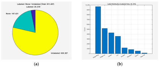
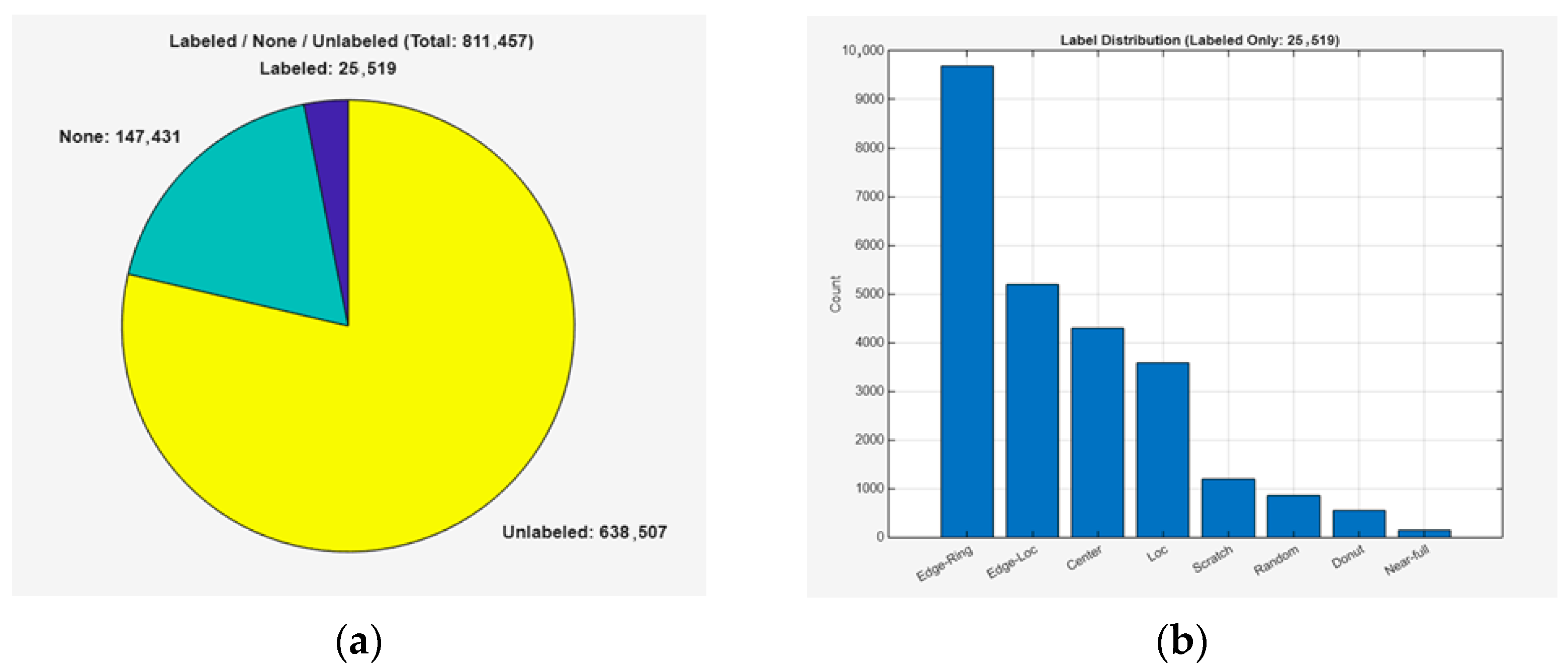
From the WM-811K benchmark dataset, unlabeled data which cannot be used for prediction were removed from the initial dataset. Next, two classes that do not contain consistent patterns or defects and were deemed irrelevant to the analytical objective, namely ‘None’ (no defect) and ‘Random’ (random noise), were excluded. Subsequently, the wafer map size of 26 × 26—the only common format across all failure types—was set as the standard. From a manufacturing standpoint, this standardization is also reasonable because wafer bin maps are die-level discrete grids, and location-dependent analyses (e.g., center/edge tendency and zone-wise density features) assume a consistent lattice geometry. Mixing different grid sizes can discretize the same physical defect distribution differently, which may bias quantitative feature extraction and the resulting rule thresholds. Based on this criterion, 200 samples were extracted for each failure type. When 26 × 26 samples were insufficient for a class, we additionally included near-sized wafer maps and converted them to 26 × 26 using a consistent preprocessing procedure. Table 1 shows the number of samples per label in the original WM-811K dataset, and Figure 2 illustrates the overall data distribution. In Figure 2a, the proportions of labeled, unlabeled, and ‘None’-labeled data are visualized using a pie chart, while Figure 2b provides a bar graph showing the distribution of labeled samples across different failure types.

Table 1. Number of labeled WBMs in WM-811K.

Failure Type	Number of Samples
Center	4294
Donut	555
Edge-Loc	5189
Edge-Ring	9680
Loc	3593
Near-full	149
Scratch	1193

Figure 2. Data distribution of WM-811K: (a) Pie chart for labeling status information; (b) Number of data per each failure type.

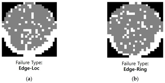
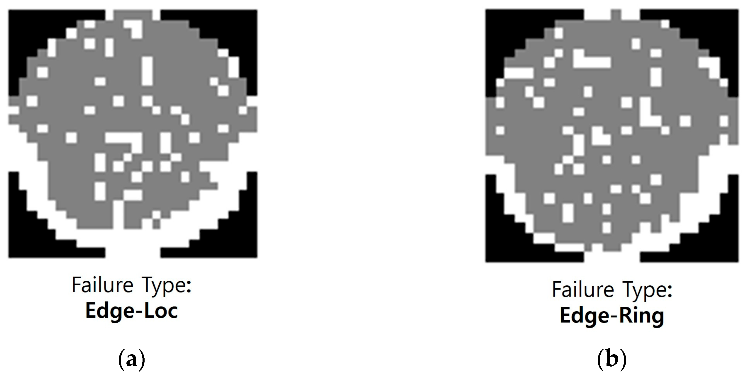
Additionally, mislabeled data (label noise) were further identified and removed through expert validation. The expert validation was conducted by two qualified evaluators: one current industry practitioner with over 20 years of experience in semiconductor defect analysis and one academic researcher in the related field. The final decisions were made through a joint review process, where both experts examined the representative patterns together and reached an agreed label based on the consistently observable spatial characteristics. Figure 3 presents representative examples of label noise. In Figure 3a, it shows the failure type of this wafer map labeled as “Edge-Loc,” whereas Figure 3b is labeled as “Edge-Ring”. Despite exhibiting highly similar spatial defect distributions, the two samples have been assigned different labels, and such inconsistency may cause boundary ambiguity during model training. Therefore, these samples were excluded from the training set to prevent overfitting and performance degradation resulting from reduced label quality. In practical manufacturing environments, however, the boundary between visually similar defect types may not be universal: the criteria used to separate closely related patterns can vary across fabrication lines and products depending on root-cause analysis and corrective actions. For this reason, the subsequent rule-based model is designed to support expert-guided adjustment of decision thresholds, enabling alignment with process-specific defect taxonomies.

Figure 3. WBM images that are incorrectly labeled: (a) WBM of failure type ‘Edge-Loc’; (b) WBM of failure type ‘Edge-Ring’.

As a result, a total of 888 samples were constructed as the initial dataset for analysis. Table 2 illustrates the label-wise data distribution after the removal of unnecessary samples and data sampling from experts. This sampling strategy was designed not only to avoid excessive concentration of data at specific sizes but also to ensure that all failure types are represented in a balanced manner.

Table 2. Number of labeled WBMs after sampling.

Failure Type	Number of Samples
Center	169
Donut	83
Edge-Loc	154
Edge-Ring	112
Loc	97
Near-full	149
Scratch	124

3.1.2. Noise Removal and Normalization

In the WM-811K dataset, each wafer map is represented as a matrix, where each cell corresponds to an individual die and is encoded using three values: ‘1’ for a normal die, ‘2’ for a defective die, and ‘0’ for regions outside the wafer area.

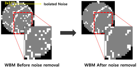
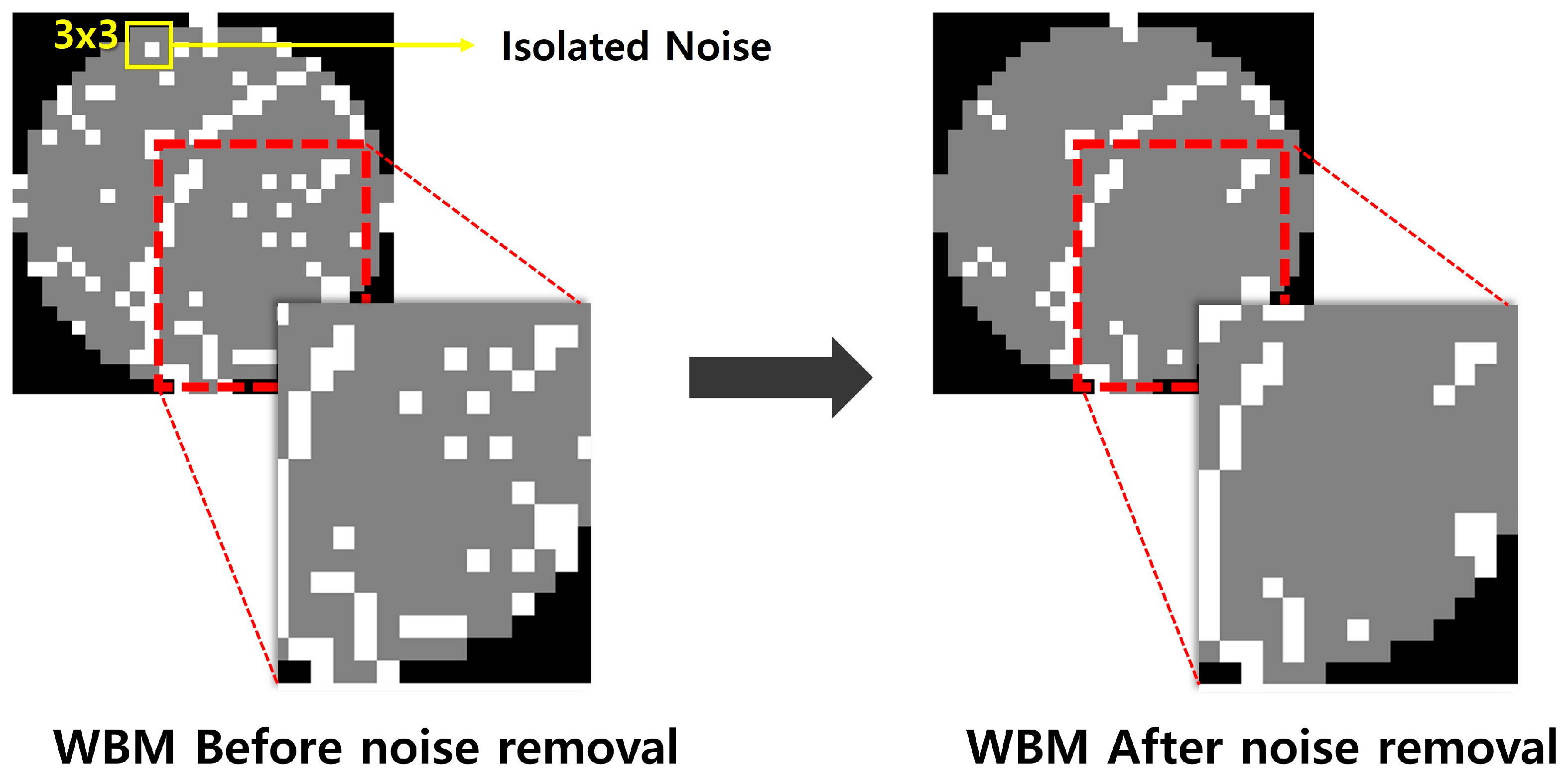
To eliminate small-scale noise and sporadic defects that could hinder analysis within the sampled data, a filtering algorithm was applied. The noise filtering algorithm used in this study is a spatial filtering technique that treats a single defective die or a small cluster of defects as noise and removes them. For each wafer map, all dies were iterated over, and a 3 × 3 local region centered on the target die was defined.

The following is the process of the proposed noise removal algorithm. First, the number of defective dies within the 3 × 3 region is counted. If the number is below a predefined threshold, the central die is likely to be noise rather than a true defect. When this condition is satisfied, and only if the central die is located within the wafer region, its value is replaced with a normal die (value = 1). In this experiment, the threshold was set to 3. Although the 3 × 3 neighborhood method is simple and effective for removing random noise in WBM, the denoising level is sensitive to the threshold: a small value may leave noise, whereas a large value may remove true defect structures and degrade classification performance. Thus, we set the threshold heuristically by calibrating it on representative thin, linear “scratch”-like patterns that traverse the wafer map, so that narrow defect structures were not overly removed. Developing a robust, WBM-specific procedure for selecting this threshold remains an important direction for future work.

As shown in Figure 4, this process effectively removes small noise or isolated defects caused by measurement errors or external factors, while preserving meaningful defect clusters that arise from actual process anomalies. Subsequently, all wafer maps were resized to 26 × 26 to standardize the input format for the model, completing the normalization process.

Figure 4. Example of WBM images before and after noise removal using a 3 × 3 neighborhood rule (threshold = 3).

3.1.3. Data Selection and Augmentation

In this study, to clearly evaluate the performance of a single-pattern classifier based on fuzzy logic, 293 samples were selected through expert review, each representing the most typical characteristics of its corresponding failure type. Table 3 presents the distribution of the selected 293 samples across different failure types.

Table 3. Number selected typical WBMs for single-pattern classification.

Failure Type	Number of Samples
Center	10
Donut	11
Edge-Loc	41
Edge-Ring	35
Loc	12
Near-full	149
Scratch	35

Subsequently, to alleviate data imbalance commonly encountered in practical environments and to enhance the generalization capability of the model, data augmentation techniques such as rotation and mirroring were applied to the selected 293 samples. As a result, a total of 749 single-pattern training samples were obtained. Table 4 presents the distribution of the 749 samples across failure types after sampling and augmentation.

Table 4. Number typical WBMs after data augmentation.

Failure Type	Number of Samples
Center	100
Donut	100
Edge-Loc	100
Edge-Ring	100
Loc	100
Near-full	149
Scratch	100

3.2. Single-Pattern Classifier Based on a Fuzzy Inference System (FIS)

3.2.1. Quantitative Feature Extraction and FIS Design

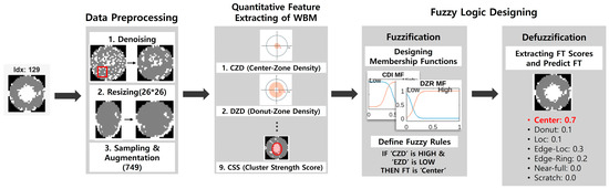
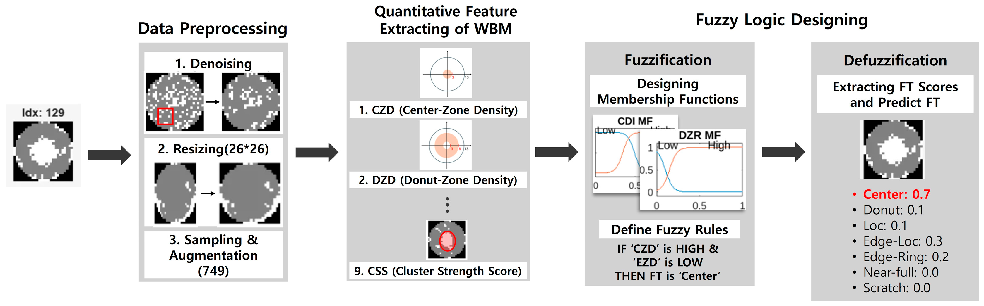
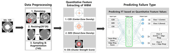
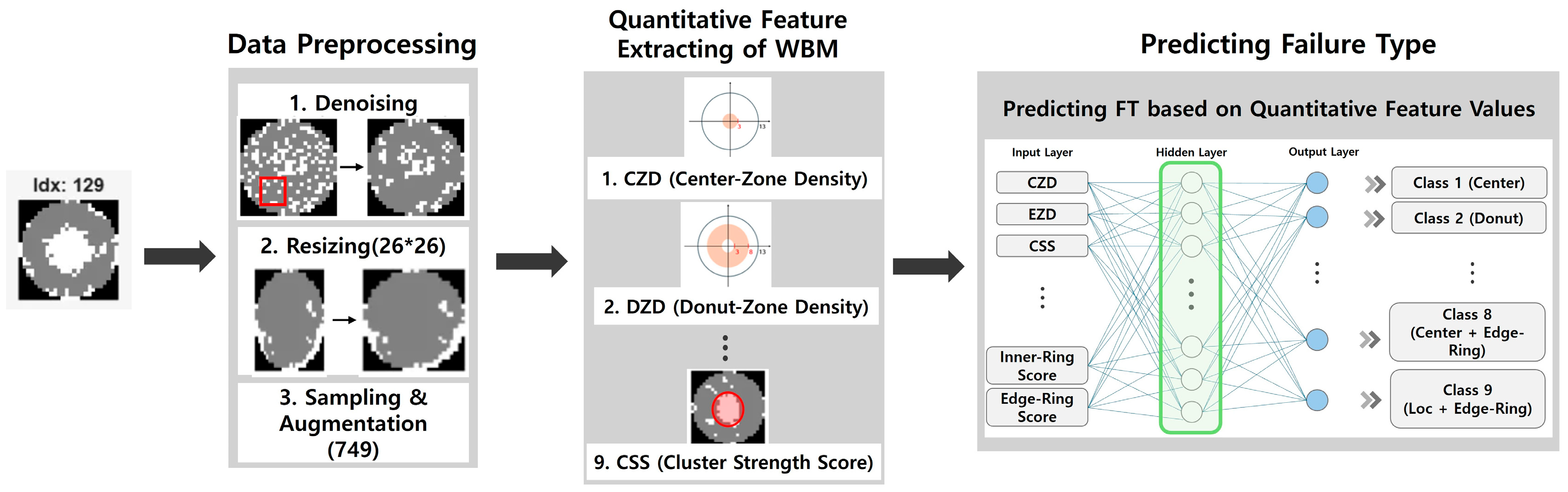
Figure 5 illustrates the flowchart of the single-pattern classification FIS model based on quantitative features. In order to effectively apply the constructed dataset to the FIS, it is first necessary to convert the visual information of wafer maps into quantitative numerical values. From the 749 preprocessed wafer maps, nine quantitative features capturing the geometric and statistical characteristics of defect patterns were extracted (e.g., Center Zone Density, Edge Zone Density, etc.).

Figure 5. Flowchart of a single-pattern FIS classification model using quantitative features.

The ‘Center Defect Density (CZD)’ is defined as the proportion of defective dies occurring in the central region of the wafer and is used to quantitatively measure center-concentrated defect patterns. It is calculated as the proportion of defective dies (=2) among valid dies within the central region (radius ≤ 4). The ‘Donut Zone Density (DZD)’ serves as a metric for evaluating the presence of donut-shaped patterns by quantifying the distribution of defects within the mid-radius region (donut region) and it is computed as the ratio of defective dies to valid dies in the range 3 < radius ≤ 8. The ‘Edge Zone Density (EZD)’ represents the defect occurrence ratio in the outer edge region of the wafer and serves as a key metric for distinguishing between edge-loc and edge-ring patterns and it is calculated as the proportion of defective dies among valid dies in the region 10 < radius ≤ 14. The ‘Inner-Ring Score’ measures how uniformly defects are distributed in the angular direction within the donut region, thereby quantifying the angular symmetry of donut-type patterns. The ‘Edge-Ring Score’ quantifies the strength of edge-ring patterns by averaging the defect density observed in the outer (edge) region of the wafer. The ‘Cluster Strength Score (CSS)’ evaluates how densely defective dies are aggregated within a local 3 × 3 window, quantitatively expressing the degree of defect clustering. The ‘Aspect Ratio and Major axis Length (ARML)’ assesses the length and linearity of scratch-type defects by utilizing the aspect ratio and major axis length of the defect region, thereby quantifying the strength of linear patterns. The ‘Average Distance’ reflects the average radial position of defects by normalizing the distance of each defective die from the wafer center using the maximum valid radius; it expresses the radial tendency of defect distribution (center-type, intermediate-ring, or edge-type) as a continuous value. The ‘Defect Density’ represents the proportion of defective dies among valid dies within the wafer, quantitatively expressing the overall level of defect amount. Table 5 presents the information on the quantitative features defined in this study.

Table 5. Name and description of the defined quantitative features extracted from the WBM.

Name	Description
CZD (Center Zone Density)	The proportion of defective dies (=2) among valid dies within the central region of the wafer (radius ≤ 4).
DZD (Donut Zone Density)	The ratio of defective dies to valid dies in the donut region (3 < radius ≤ 8).
EZD (Edge Zone Density)	The proportion of defective dies among valid dies in the edge region (10 < radius ≤ 14).
Inner-Ring Score	An axis-symmetry metric that indicates how uniformly defects are distributed in the angular direction within the donut region.
Edge-Ring Score	A metric that quantifies the strength of the Edge-Ring pattern by averaging the defect density in the outer-radius region.
CSS (Cluster Strength Score)	A metric that represents defect density by normalizing the degree of clustering within a local 3 × 3 region.
ARML (Aspect Ratio, Major axis Length)	A metric that evaluates the strength of linear (scratch-type) defects based on the aspect ratio and major axis length of the defect region.
Average Distance	A metric that represents the radial tendency of defect locations, calculated as the average distance of defective dies from the center normalized by the maximum radius.
Defect Density	An overall defect quantity metric that indicates the ratio of defective dies to valid dies within the wafer.

To analyze the distribution of these extracted features, boxplots and histograms were employed. Based on the results of this statistical analysis, a single fuzzy inference system (FIS) was designed to output classification scores for each of the seven failure types.

3.2.2. Fuzzy Rule Design and Activation Strength Computation

The fuzzy rules were defined within the designed FIS to produce seven defect pattern outputs. Table 6 provides a detailed description of the eight rules used in the single-pattern classifier. The rule construction was based on human-perceivable characteristics observed when interpreting wafer maps (e.g., defect location, distribution, and density), and was optimized through iterative comparison and calibration with statistical indicators and experimental results. For each wafer map, the firing strength of each rule was calculated, and the highest activation value among the rules associated with each defect class was defined as the score of that class. The final prediction was determined as the failure type with the highest score among all classes.

Table 6. Fuzzy rules of the FIS based single-pattern classification model.

Rule	CZD	DZD	EZD	CSS	Inner-Ring Score	Edge-Ring Score	ARML	Average Distance	Defect Density	Class
R1	High	-	Low	High	Low	Low	-	-	-	Center
R2	Low	High	Low	-	High	Low	-	-	Low	Donut
R3	Low	-	High	High	Low	Low	-	-	Low	Edge-Loc
R4	Low	Low	High	Low	Low	High	High	-	-	Edge-Ring
R5	Low	Low	High	Low	Low	-	High	Edge	-	Edge-Ring
R6	-	-	-	-	-	-	-	-	High	Near-full
R7	-	-	-	Low	-	Low	High	Central	Low	Scratch
R8	-	High	-	High	Low	Low	Low	-	Low	Loc

Traditional defuzzification methods (e.g., centroid or bisector) were not used for the following reasons:

• Nature of the output space: The output of this task consists of seven nominal categories rather than a continuous scalar value. Applying conventional defuzzification would require assigning arbitrary numeric codes to these categories, which introduces artificial distance metrics and causes geometric distortion;
• Limitations in representing composite or overlapping patterns: Real wafer defects often contain more than one pattern simultaneously. Single scalar defuzzification collapses such multi-activation states into a single value, leading to the loss of secondary pattern information;
• Interpretability: Maximum firing strength directly reveals which rule was activated and why, making it more suitable for cause tracing and visual interpretation than MATLAB R2025a’s automated defuzzification results.

3.2.3. Analysis of the Structural Limitations of the Single-Pattern Classifier

To verify the practical applicability of the single-pattern classifier, it was applied to a separate dataset consisting of 888 samples that contain atypical or composite patterns. The composition of this dataset is summarized in Table 7. The fuzzy rules of the single-pattern classifier were designed under the assumption that each failure type appears in its typical form. For example, the rule for the “Center” type is constructed based on a clear condition such as “the defect density in the center region is high, while that in the outer region is low.”

Table 7. Number of WBMs with atypical defect pattern for FIS based single-pattern classification.

Failure Type	Number of Samples
Center	169
Donut	83
Edge-Loc	154
Edge-Ring	112
Loc	97
Near-full	149
Scratch	124

In contrast, wafer maps observed in actual manufacturing processes may exhibit atypical variations, such as an abnormally wide central defect area or a slightly shifted center. In such cases, the input data may fail to fully satisfy the antecedent conditions of the rules, resulting in ambiguous classification. This limitation becomes particularly evident in the presence of composite patterns, where high defect densities may simultaneously occur across multiple regions, making it difficult to reach a decision using typical rule-based approaches. For instance, when “Center” and “Edge-Loc” patterns appear concurrently, the corresponding rule conditions of both classes are partially violated, leading to weak membership in both categories.

This analysis indicates that a traditional FIS-based single-pattern classifier may exhibit structural limitations when faced with complex and atypical defect patterns, highlighting the need for an extended classification strategy to address these cases. To experimentally validate these theoretical limitations, the model performance was evaluated using the dataset containing 888 atypical and composite patterns. The results are presented in detail in Section 4.

3.3. Composite-Pattern Classifier

To overcome the limitations of the single-pattern classifier, this study compares the performance of three composite-pattern classifiers: a hybrid model that integrates FIS and a neural network, a neural network model that directly utilizes quantitative features, and a CNN model that uses the raw 2D WBM images.

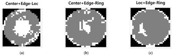
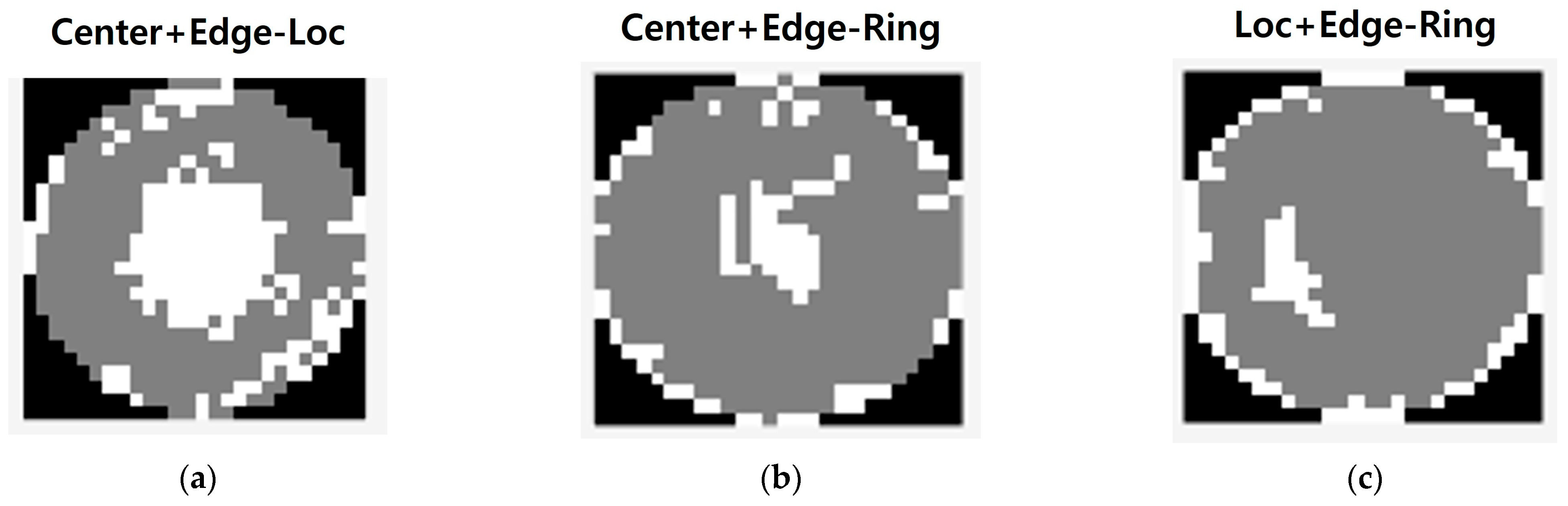
To accomplish this, expert validation was conducted to assign labels for the three representative composite patterns—Center+Edge-Loc, Center+Edge-Ring, and Loc+Edge-Ring—that were consistently and repeatedly observed within the 26 × 26 standardized subset used in this study. These labels were integrated into the existing dataset of 888 samples to construct an updated dataset. Figure 6 shows WBM images of the additionally labeled composite patterns. Figure 6a corresponds to the Center+Edge-Loc label, where defects are concentrated in both the central region and the irregular edge region. Figure 6b depicts the Center+Edge-Ring label, where uniform ring-shaped defect patterns occur in both the center and edge regions. Figure 6c shows the Loc+Edge-Ring label, where uniform ring-shaped defects are distributed across the intermediate region between the center and edge of the wafer, as well as the edge region itself.

Figure 6. Example WBM images of the three representative composite defect patterns: (a) Center+Edge-Loc; (b) Center+Edge-Ring; (c) Loc+Edge-Ring.

To address data imbalance within the composite-pattern classes, augmentation techniques were applied, resulting in a final dataset of 1134 samples for composite-pattern training. Table 8 presents the distribution of the dataset including composite defect pattern labels.

Table 8. Number of WBM samples containing composite defect pattern labels.

Failure Type	Number of Samples
Center	139
Donut	83
Edge-Loc	150
Edge-Ring	92
Loc	97
Near-full	149
Scratch	124
Center+Edge-Loc	100
Center+Edge-Ring	100
Loc+Edge-Ring	100

3.3.1. Hybrid FIS-NN Classifier

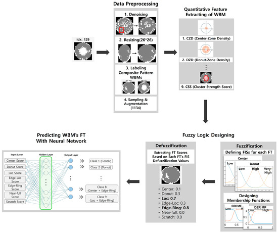
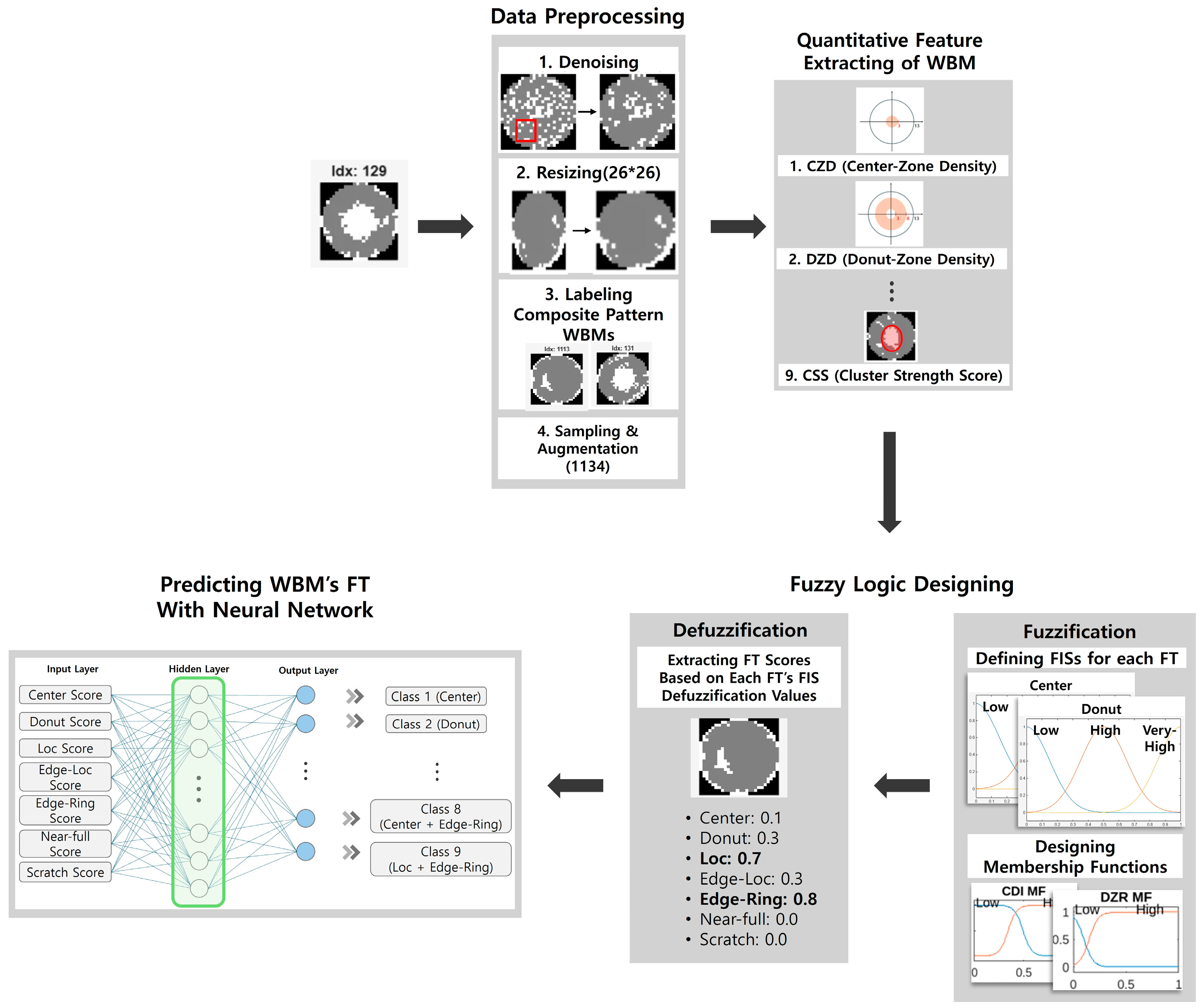
The first model that we proposed adopts a structure in which independent FIS modules are designed for each failure type to more precisely capture their characteristics. Figure 7 presents the flowchart of the hybrid FIS-NN classifier. A total of seven individual FIS modules—such as “Center FIS” and “Donut FIS”—were constructed, and the membership functions were divided into three levels: “Very High,” “High,” and “Low.” In addition, fuzzy rules were designed to reflect the properties of composite patterns (e.g., IF CZD is High AND EZD is High THEN Center Score is High). Table 9 lists the rules applied to the Center FIS. Rule 1 and Rule 2 represent a typical single-pattern case and assigns a “Very High” score, while Rules 3 through 5 consider composite patterns and assign a “High” score. Rules 6 through 7 address non-center cases and assign a “Low” score, thereby enabling the quantitative reflection of composite pattern characteristics in the final score calculation.

Figure 7. Flowchart of the hybrid FIS-NN classifier.

Table 9. Example of the Center FIS fuzzy rules in the FIS-NN classification model.

Rule	CZD	DZD	EZD	CSS	Inner-Ring Score	Edge-Ring Score	ARML	Average Distance	Defect Density	Output (Center-Score)
R1	High	-	Low	High	-	-	-	Central	-	Very-High
R2	High	High	Low	High	-	-	-	Central	-	Very-High
R3	High	-	High	-	-	High	High	-	-	High
R4	High	-	High	-	-	-	-	-	-	High
R5	-	-	-	-	-	-	-	Central	-	High
R6	Low	-	-	-	-	-	-	-	-	Low
R7	-	-	-	-	-	-	-	Edge	-	Low

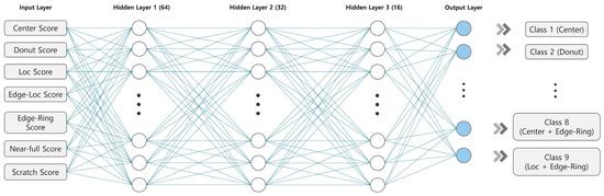
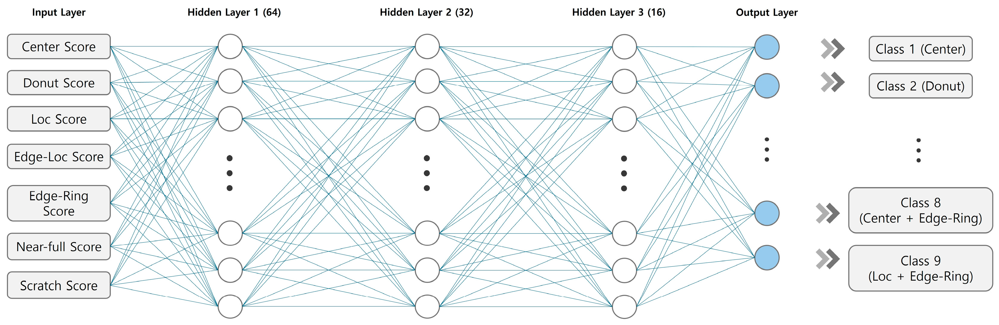
Using the seven FIS modules designed in this manner, seven scores were generated for each wafer map, and this score vector (1134 × 7) was used as the input feature for training the neural network model. Figure 8 shows the architecture of the neural network employed in this study. The network consists of three fully connected hidden layers with 64–32–16 nodes and ReLU activation functions, while the output layer performs multi-class classification using a Softmax function. The training process utilized the Scaled Conjugate Gradient (trainscg) algorithm and a weighted cross-entropy loss function to address class imbalance. Additionally, early stopping with a max_fail criterion of 15 was applied to prevent overfitting. The data were divided into Train:Validation:Test sets with a ratio of 6:2:2.

Figure 8. Structure of neural network for proposed FIS-NN classification model.

3.3.2. Quantitative Feature-Based NN Classifier

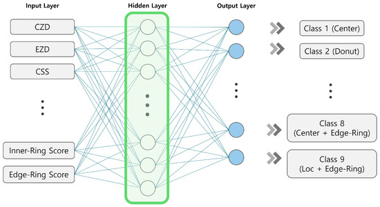
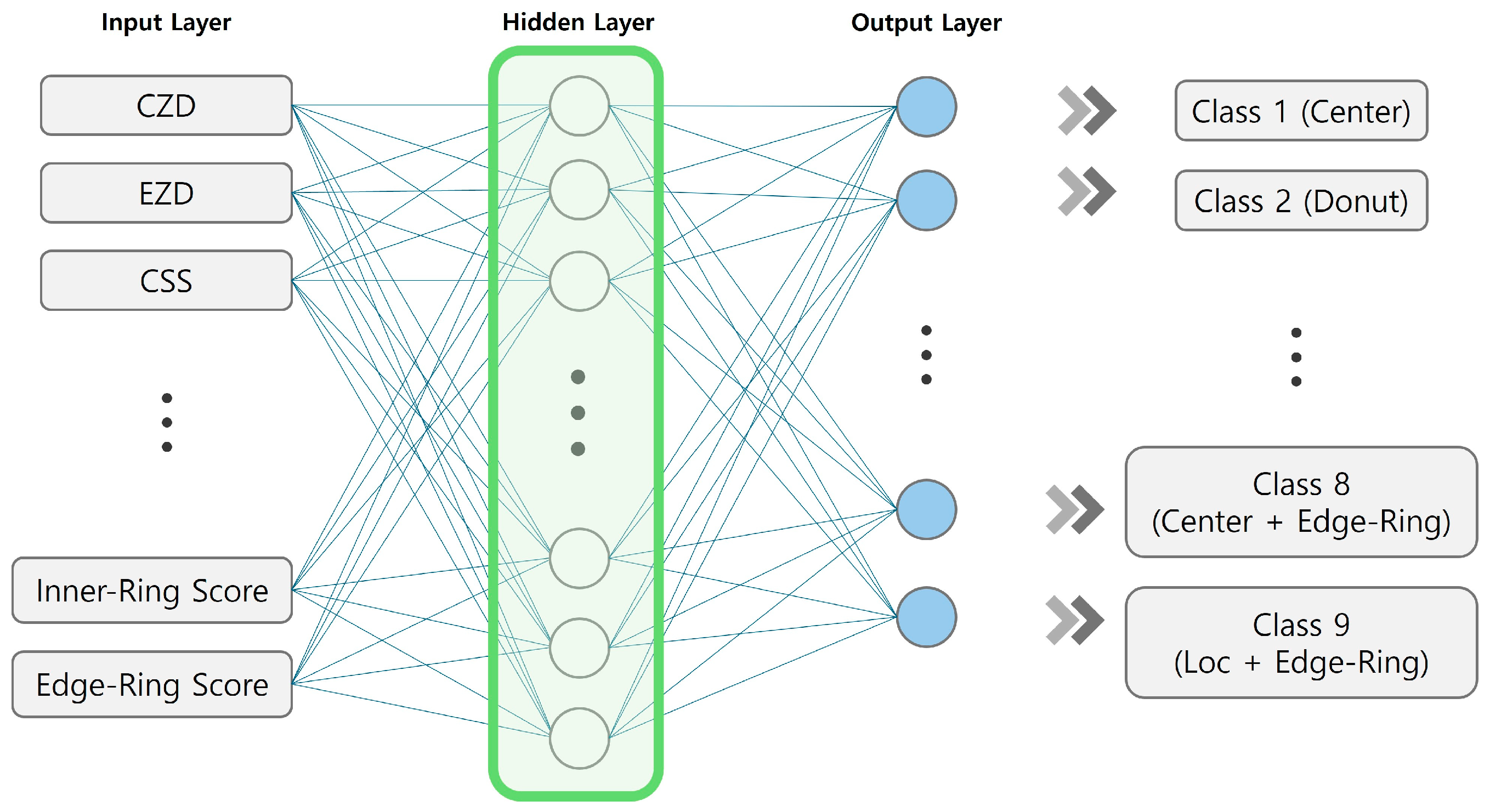
The second model bypasses the FIS and directly uses the nine quantitative features extracted from the data as inputs to the neural network. This approach is intended to fully exploit the information contained in the original features without the potential information loss that may occur during the fuzzification process. Figure 9 illustrates the procedure of the feature-based NN classification. The names and detailed descriptions of each feature are provided in Table 5. The input data thus take the form of 1134 × 9, while the neural network architecture and training conditions, excluding the input layer, were kept identical to those of the first model. Figure 10 shows the architecture of the NN.

Figure 9. Flowchart of quantitative feature-based NN classifier.

Figure 10. Structure of NN in quantitative feature-based NN classifier.

3.3.3. Convolutional Neural Network Classifier Based on Raw WBMs

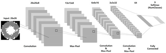
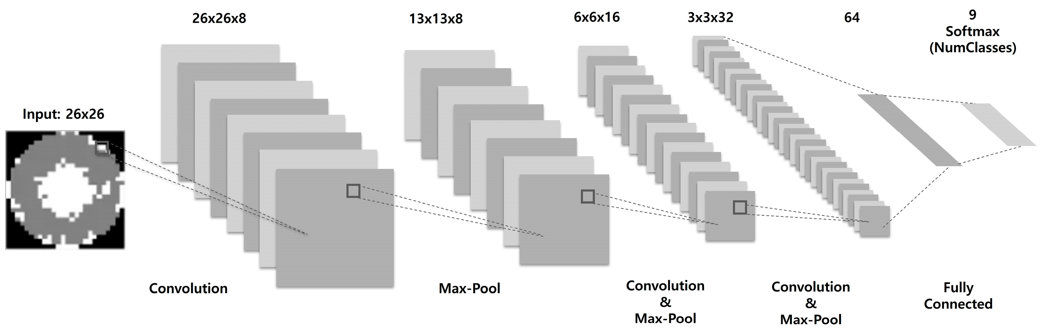
Lastly, a convolutional neural network (CNN) was constructed to directly learn the spatial patterns of the original wafer maps by omitting the feature extraction step. The CNN-based classifier takes a 26 × 26 wafer map image as input, and extracts spatial features through three Convolution–BatchNorm–ReLU blocks and two MaxPooling layers. This is followed by a fully connected layer with 64 nodes and a Dropout layer (0.3) to enhance generalization performance, and finally, multi-class classification is performed using a Softmax layer. Training was conducted using the Adam optimization algorithm with a mini-batch size of 64 over 50 epochs. The dataset was split into Train/Validation/Test sets with a ratio of 6:2:2. Figure 11 illustrates the CNN architecture used in this study.

Figure 11. Structure of CNN.

4. Results

In this study, experiments were conducted and performance was compared across five scenarios summarized in Table 10, based on the type of input data and the structure of the classifier. These scenarios were categorized into single-pattern classifiers and composite-pattern classifiers according to the defect classification objective, and particular attention was paid to analyzing the differences in learning methods depending on whether the input format was feature-based or image-based. Three comparison groups were constructed according to the model design objectives and input structures.

Table 10. Summary of the four models used to classify WBM defect patterns.

Model Number	Input Type	Model Type	Objective
1	9-D quantitative feature vector (typical WBMs)	Single FIS (multi-class classifier)	for classification of single failure pattern
2	9-D quantitative feature vector (atypical WBMs)	Single FIS (multi-class classifier)	for classification of single failure pattern
3	9-D quantitative feature vector (composite defect labels)	Multiple FISs (one per Failure Type) +NN	for classification of composite failure pattern
4	9-D quantitative feature vector (composite defect labels)	NN	for classification of composite failure pattern
5	WBM images	CNN	for classification of composite failure pattern

The first group (Model 1 vs. Model 2) employed the same multi-class FIS structure but examined whether classification performance differed depending on whether the input data were typical or atypical WBMs. This experiment aimed to verify the generalization capability of the proposed 9-D quantitative feature vector.

The second group (Model 3 vs. Model 4) compared feature-based classifiers for composite defect labels, specifically contrasting a hybrid structure with independent FIS modules for each failure type (FIS+NN) against a single neural network model. This comparison was designed to analyze whether using FIS as a feature extractor is effective for detecting composite patterns.

The third group (Model 4 vs. Model 5) evaluated the structural differences between feature-based and image-based end-to-end approaches by comparing a feature-based NN with a CNN model that takes raw WBM images as input. Through these group-wise comparisons, the relative advantages of feature engineering-based approaches and automatic feature learning-based approaches were experimentally analyzed for the wafer map classification problem.

To quantitatively compare the performance of the four proposed models, four evaluation metrics—Accuracy, Precision, Recall, and F1-Score—were employed. These metrics are calculated based on the values of TP (True Positive), TN (True Negative), FP (False Positive), and FN (False Negative) contained in the confusion matrix, and are defined by Equations (1)–(4).

$$\mathrm{A}\mathrm{c}\mathrm{c}\mathrm{u}\mathrm{r}\mathrm{a}\mathrm{c}\mathrm{y}={\displaystyle \frac{\mathrm{T}\mathrm{P}+\mathrm{T}\mathrm{N}}{\mathrm{T}\mathrm{P}+\mathrm{F}\mathrm{N}+\mathrm{F}\mathrm{P}+\mathrm{T}\mathrm{N}}}$$

(1)

$$\mathrm{P}\mathrm{r}\mathrm{e}\mathrm{c}\mathrm{i}\mathrm{s}\mathrm{i}\mathrm{o}\mathrm{n}={\displaystyle \frac{\mathrm{T}\mathrm{P}}{\mathrm{T}\mathrm{P}+\mathrm{F}\mathrm{P}}}$$

(2)

$$\mathrm{R}\mathrm{e}\mathrm{c}\mathrm{a}\mathrm{l}\mathrm{l}={\displaystyle \frac{\mathrm{T}\mathrm{P}}{\mathrm{T}\mathrm{P}+\mathrm{F}\mathrm{N}}}$$

(3)

$$\mathrm{F}1-\mathrm{S}\mathrm{c}\mathrm{o}\mathrm{r}\mathrm{e}={\displaystyle \frac{2\times \mathrm{P}\mathrm{r}\mathrm{e}\mathrm{c}\mathrm{i}\mathrm{s}\mathrm{i}\mathrm{o}\mathrm{n}\times \mathrm{R}\mathrm{e}\mathrm{c}\mathrm{a}\mathrm{l}\mathrm{l}}{\mathrm{P}\mathrm{r}\mathrm{e}\mathrm{c}\mathrm{i}\mathrm{s}\mathrm{i}\mathrm{o}\mathrm{n}+\mathrm{R}\mathrm{e}\mathrm{c}\mathrm{a}\mathrm{l}\mathrm{l}}}$$

(4)

4.1. Comparison of Classifier Performance in Single Failure Pattern

To evaluate the classification performance for single failure patterns, the Model 1 and the Model 2 were compared. Although both models employ the same FIS structure, they differ in the characteristics of the input data. The datasets used for each model are presented in Table 4 and Table 7, respectively. The Model 1 used 9-dimensional quantitative feature vectors extracted from typical WBMs, whereas Model 2 is designed to train on the same set of features extracted from atypical WBMs. Through this comparison, the generalization capability of the proposed feature-based approach under changes in the data domain was experimentally validated.

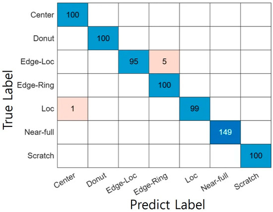
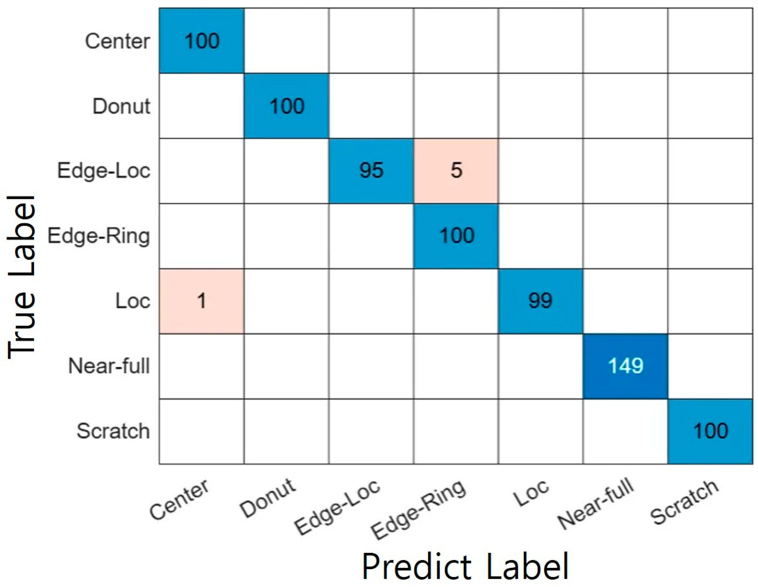
Based on the evaluation of Model 1, a classification accuracy of 99.20% was achieved on 749 samples exhibiting typical (single-type) defect characteristics. Figure 12 shows the confusion matrix of the Model 1, where the x-axis represents the predicted failure types and the y-axis represents the actual failure types. These results confirm that, for clearly defined typical samples, predictions based on the activation strength of fuzzy rules (rule strength values) derived from quantitative features are effective for WBM analysis.

Figure 12. Confusion Matrix of Model 1.

Consequently, the single-pattern classifier demonstrated both high quantitative performance and interpretability through its explicit rule-based structure. Unlike black-box neural networks, this approach enables engineers to intuitively understand the underlying causes of defect patterns and the influential variables associated with them. This suggests the potential use of the proposed model as a knowledge-driven classification framework for future composite-pattern detection and process anomaly diagnosis.

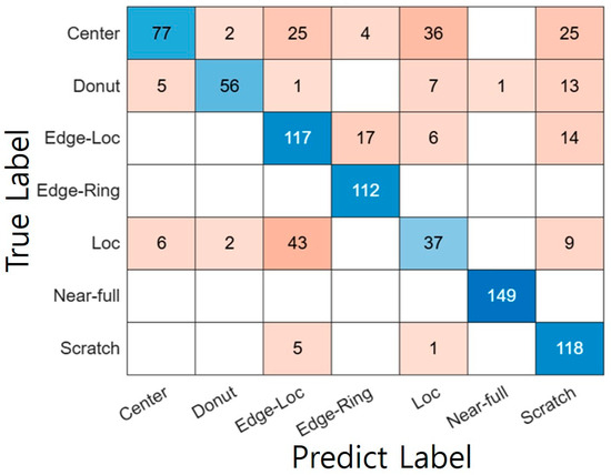
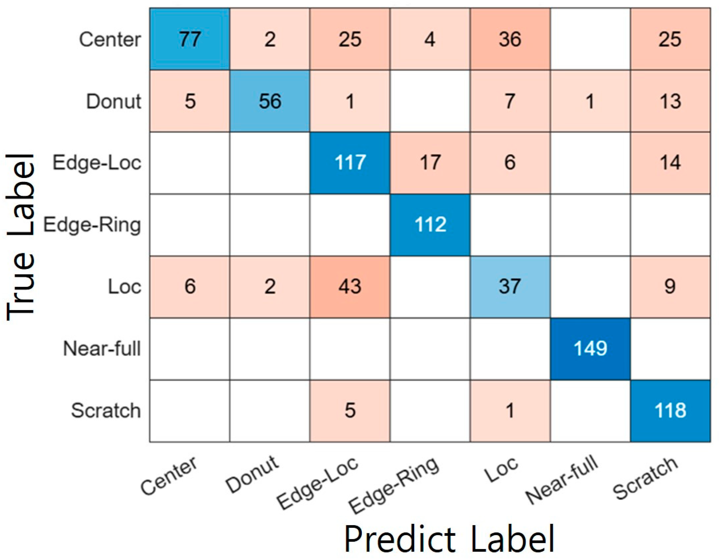
However, to verify the practical effectiveness of the Model 1, the Model 2 was applied to a separate dataset consisting of 888 samples that included atypical or composite patterns. As a result, the accuracy dropped significantly to 75%. Figure 13 shows the confusion matrix of the single-pattern classifier when classifying the dataset containing atypical patterns. This performance degradation stems from the following structural limitations of the single-pattern classifier. As shown in Table 6, the rules of the single-pattern FIS were designed under the assumption that each defect appears in its typical form. For example, the rule for the “Center” type is defined as “the defect density in the center region is high (High), and that in the outer region is low (Low).”

Figure 13. Confusion Matrix of Model 2.

However, in real data, atypical cases frequently occur in which the central defect area is abnormally wide or slightly shifted from the center, and in such cases, the antecedent conditions of the rules are only partially satisfied, leading to incorrect classifications. This limitation becomes even more evident in the presence of composite patterns. For instance, a pattern combining “Center” and “Edge-Loc” exhibits high defect densities in both the central and certain edge regions. When such a sample is input to the single-pattern classifier, the “Center” rule outputs a low score because it violates the condition that the edge region must have low density, while the “Edge-Loc” rule also yields a low score due to the condition that the central defect density must be low. Consequently, both types receive low scores, or an unexpected third type is predicted as having the highest score. Table 11 presents a one-to-one comparison between the Model 1 and the Model 2. This analysis clearly demonstrates that the rule-based single-pattern classification approach has structural limitations in detecting composite patterns, thereby highlighting the need for a new approach to address this issue.

Table 11. Comparison of classification model performances for single failure patterns.

Failure Type	Model 1			Model 2
	Precision	Recall	F1-Score	Precision	Recall	F1-Score
Center	0.99	1	0.99	0.88	0.46	0.6
Donut	1	1	1	0.93	0.67	0.78
Edge-Loc	1	0.95	0.97	0.64	0.75	0.69
Edge-Ring	0.95	1	0.97	0.84	1	0.91
Loc	1	0.99	1	0.73	0.38	0.5
Near-full	1	1	1	0.99	1	1
Scratch	1	1	1	0.66	0.94	0.78
Average	0.99	0.99	0.99	0.81	0.74	0.75

4.2. Comparison of Classifier Performance in Composite Failure Pattern

To analyze the classification performance for composite failure patterns, Model 3, Model 4 and Model 5 were compared. As described in Section 4.1, in real manufacturing processes, cases where two or more defect patterns appear simultaneously are frequently observed, and such patterns possess characteristics that are difficult to accurately classify using a single rule-based approach. Table 12 presents a one-to-one comparison of the three models. In addition, Table 13 summarizes the computational cost of each model, including inference latency and model footprint, measured in a consistent MATLAB Online environment (batch size = 1, warm-up followed by timeit, reported as mean ± standard deviation over N = 100 test samples).

Table 12. Comparison of classification model performances for composite failure patterns.

Failure Type	Model 3			Model 4			Model 5
	Precision	Recall	F1-Score	Precision	Recall	F1-Score	Precision	Recall	F1-Score
Center	0.87	0.96	0.91	0.88	0.85	0.86	0.73	0.92	0.82
Center+Edge-Loc	0.82	0.9	0.86	0.86	0.9	0.88	1	0.4	0.57
Center+Edge-Ring	0.88	1	0.93	0.91	1	0.95	0.95	1	0.98
Donut	1	0.89	0.94	1	0.9	0.95	1	0.95	0.97
Edge-Loc	0.76	0.79	0.78	0.90	0.93	0.92	0.83	0.8	0.81
Edge-Ring	1	0.90	0.95	0.94	0.89	0.91	0.78	0.95	0.86
Loc	0.68	0.75	0.71	0.78	0.67	0.72	0.85	0.61	0.71
Loc+Edge-Ring	0.96	0.93	0.95	0.96	0.93	0.95	0.95	0.74	0.83
Near-full	1	1	1	1	1	1	1	1	1
Scratch	0.8	0.76	0.78	0.91	0.86	0.88	0.68	0.72	0.7
Average	0.88	0.90	0.88	0.91	0.89	0.88	0.87	0.81	0.82

Table 13. Comparison of computational cost of three models.

Model Number	Timing Scope	Inference Time (ms)	Model Size (MB)	Parameters
3	Classifier stage (vector → output)	3.742 ± 0.099	0.26	3290
4	Classifier stage (vector → output)	3.768 ± 0.266	0.26	3418
5	End-to-end (image → output)	1.092 ± 0.050	0.49	80,442

4.2.1. Comparison of Feature-Based Classifiers (Model 3 vs. Model 4)

The Model 3 was designed as a hybrid structure based on expert-reviewed composite defect labels, using a 9-dimensional quantitative feature vector as input and independent FIS modules for each failure type. The firing strengths computed from each FIS were then converted into a feature vector and fed into a neural network. In contrast, Model 4 directly inputs the same quantitative features (9-D feature vector) into the neural network without using FIS as a feature extractor, which constitutes a structural difference between the two approaches. The data distributions used for both models are presented in Table 8.

Although both models follow a feature-based architecture, they serve as a significant comparison target in terms of whether FIS—an expert knowledge-based rule system—should be utilized as a feature extractor. This distinction can impact the classification performance and generalization capability. In this section, performance metrics including Accuracy, Precision, Recall, and F1-Score and confusion matrices were used to analyze the characteristics and limitations of the two models and to verify whether FIS-based feature extraction contributes to tangible performance improvements in the classification of composite failure patterns.

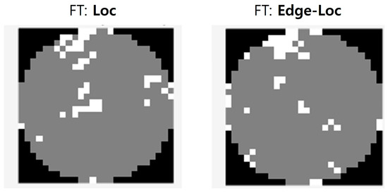
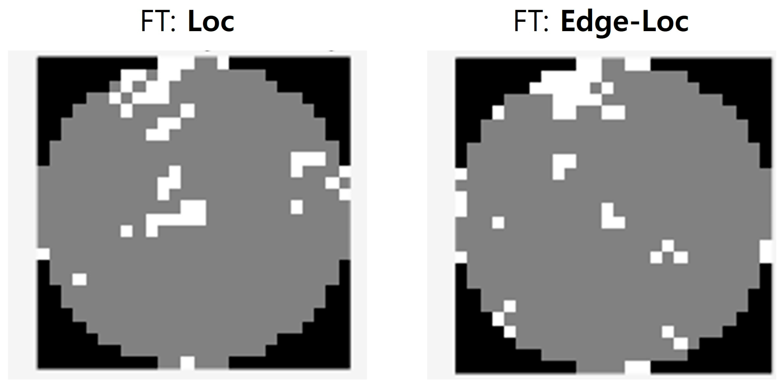
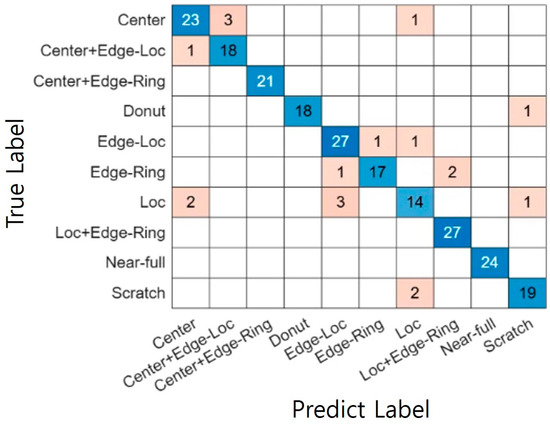
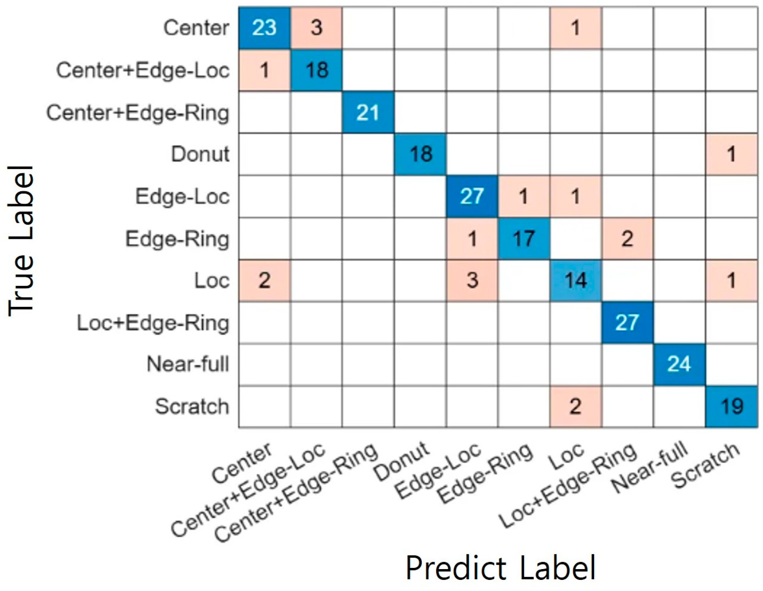
Based on the evaluation of the Model 3, the hybrid model achieved a classification accuracy of 88.55%. Figure 14 presents the confusion matrix of the Model 3 and relatively low classification accuracy was observed for Edge-Loc, Loc, and Scratch types, which appears to be attributable to labeling uncertainty in some samples as well as morphological similarity among these patterns. Figure 15 illustrates examples of wafer map data that exhibit similar patterns but are labeled as different types, such as Loc and Edge-Loc. In practice, these patterns often exhibit overlapping spatial distributions of defects, making their labels susceptible to subjective variation among experts. Nonetheless, most of the other failure types showed high classification accuracy, confirming the overall effectiveness of the proposed classifier. This is likely due to the complementary interaction between fuzzy rule-based feature extraction and the nonlinear discriminative capability of the neural network, enabling effective learning of the spatial characteristics of defect patterns.

Figure 14. Confusion Matrix of Model 3.

Figure 15. Examples of WBMs with similar distributions but labeled differently in the original dataset.

For the Model 4, an accuracy of 91.63% was achieved, indicating improved performance compared to the FIS–NN hybrid model (88.55%). Figure 16 shows the confusion matrix of Model 4, the feature-based NN model. These results suggest that the nine proposed quantitative features effectively capture the complex characteristics of wafer map defects, including spatial distribution, defect density, and asymmetry. Furthermore, the high accuracy achieved without the use of fuzzy rules implies that the designed features possess sufficient physical and statistical representational power to explain the nonlinear differences between defect patterns. In other words, while the Model 4 may provide slightly lower interpretability compared to FIS-based approaches due to the absence of explicit rule-based structure, it maximizes the advantages of data-driven learning by directly utilizing the original features. In future work, it is expected that the strengths of both approaches could be combined to simultaneously enhance interpretability and predictive performance. Table 14 presents a one-to-one comparison of the two models.

Figure 16. Confusion Matrix of Model 4.

Table 14. Classification performance comparison table for the two models. (Model 3 vs. Model 4).

Failure Type	Model 3			Model 4
	Precision	Recall	F1-Score	Precision	Recall	F1-Score
Center	0.87	0.96	0.91	0.88	0.85	0.86
Center+Edge-Loc	0.82	0.9	0.86	0.86	0.9	0.88
Center+Edge-Ring	0.88	1	0.93	0.91	1	0.95
Donut	1	0.89	0.94	1	0.9	0.95
Edge-Loc	0.76	0.79	0.78	0.90	0.93	0.92
Edge-Ring	1	0.90	0.95	0.94	0.89	0.91
Loc	0.68	0.75	0.71	0.78	0.67	0.72
Loc+Edge-Ring	0.96	0.93	0.95	0.96	0.93	0.95
Near-full	1	1	1	1	1	1
Scratch	0.8	0.76	0.78	0.91	0.86	0.88
Average	0.88	0.90	0.88	0.91	0.89	0.88

4.2.2. Comparison of Feature-Based and Image-Based Classifiers (Model 4 vs. Model 5)

In this section, the Model 4 and the Model 5 were compared to analyze the structural differences between the feature-based approach and the image-based end-to-end learning approach. As described in Section 4.2.1, Model 4 is a feature-based classifier that directly inputs a 9-dimensional quantitative feature vector—derived from composite defect labels—into a neural network. The Model 5, on the other hand, minimizes preprocessing and utilizes a CNN-based architecture that takes denoised and normalized WBM images as input. The primary distinction between the two models lies in their input format and feature extraction strategy, making them a meaningful comparison for experimentally evaluating expert knowledge-based feature representation versus automatic feature learning. In this section, the performance differences between the two models were analyzed using Accuracy, Precision, Recall, F1-score, and confusion matrices, to assess whether feature engineering is fundamentally necessary for wafer map classification or whether an end-to-end structure can be more efficient. The experimental results of Model 4 are presented in detail in Section 4.2.1.

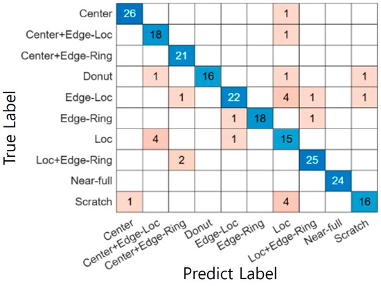
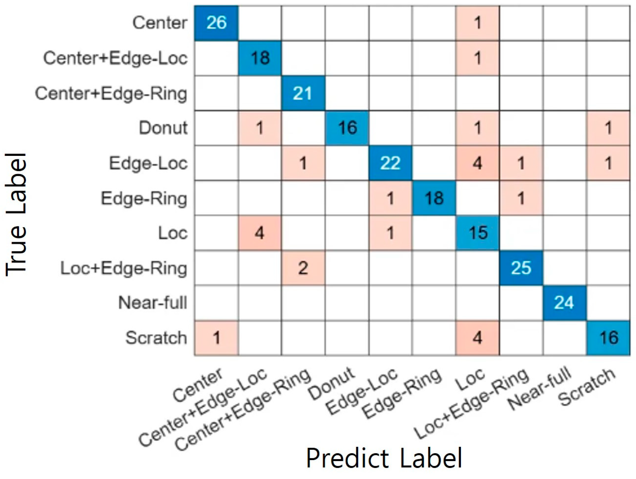
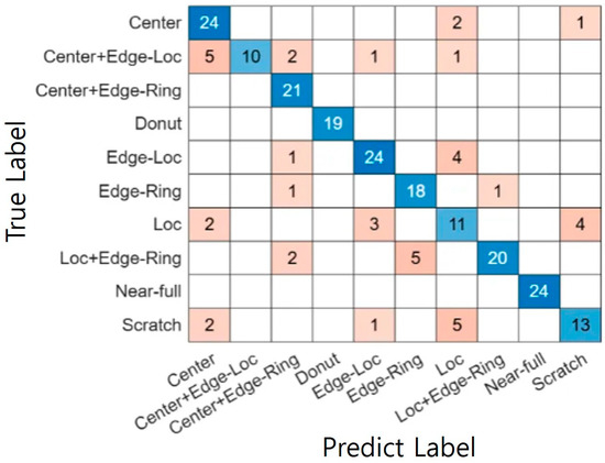
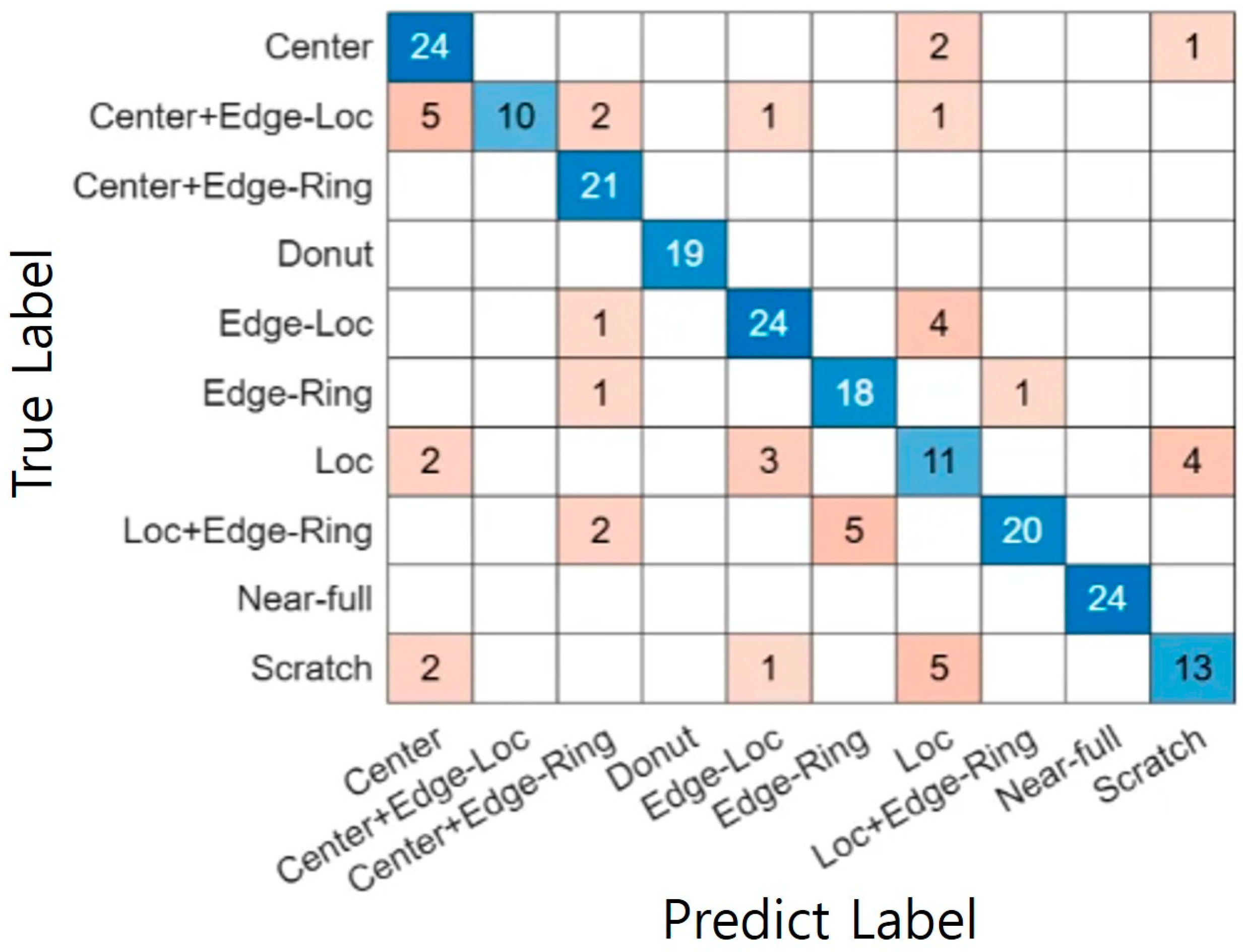
The test accuracy of the Model 5 was observed to be 81.06%, with relatively low recall particularly in the Loc, Scratch, and Center+Edge-Loc classes. Figure 17 shows the confusion matrix of model 5. This performance drop can be attributed to spatial similarity between classes and labeling ambiguity within the dataset. These patterns often exhibit overlapping defect locations or shapes, making it difficult for a standard CNN architecture to learn subtle boundary distinctions. Moreover, due to the limited number of wafer map samples and class imbalance, the CNN is structurally prone to overfitting and sensitive to label noise.

Figure 17. Confusion Matrix of Model 5.

Furthermore, the CNN exhibits a critical limitation in that its internal weights are entangled in a complex nonlinear manner, making it practically impossible to modify or tune decision rules analytically based on the results. That is, tracing the decision rationale or adjusting specific rules for individual failure types is challenging, leading to insufficient interpretability and decision transparency—both of which are essential in semiconductor process engineering applications.

These limitations further highlight the necessity of the fuzzy inference-based system (FIS) proposed in this study. By explicitly representing spatial tendencies and interrelationships of defects through fuzzy rules, the FIS enables robust and interpretable classification even in the presence of label noise or composite patterns. Table 15 presents a one-to-one comparison of the two models.

Table 15. Classification performance comparison table for the two models. (Model 4 vs. Model 5).

Failure Type	Model 4			Model 5
	Precision	Recall	F1-Score	Precision	Recall	F1-Score
Center	0.88	0.85	0.86	0.73	0.92	0.82
Center+Edge-Loc	0.86	0.9	0.88	1	0.4	0.57
Center+Edge-Ring	0.91	1	0.95	0.95	1	0.98
Donut	1	0.9	0.95	1	0.95	0.97
Edge-Loc	0.90	0.93	0.92	0.83	0.8	0.81
Edge-Ring	0.94	0.89	0.91	0.78	0.95	0.86
Loc	0.78	0.67	0.72	0.85	0.61	0.71
Loc+Edge-Ring	0.96	0.93	0.95	0.95	0.74	0.83
Near-full	1	1	1	1	1	1
Scratch	0.91	0.86	0.88	0.68	0.72	0.7
Average	0.91	0.89	0.88	0.87	0.81	0.82

5. Discussion

In this study, five models combining fuzzy inference systems (FIS), neural networks, and CNNs were designed for WM-811K wafer map classification, and their performance and limitations were compared under both single-pattern and composite-pattern scenarios. Overall, the results demonstrated that while rule-based FIS achieved exceptionally high accuracy and interpretability for typical single-pattern cases, its generalization capability diminished significantly when atypical or composite patterns were introduced. In contrast, feature-based classifiers utilizing composite labels and quantitative features outperformed the CNN-based end-to-end model in both performance and stability.

In the single-pattern classification experiments, Model 1 achieved exceptionally high performance—Accuracy of 0.99 and an average F1-score of 0.99—on typical wafer maps. This indicates that the nine-dimensional quantitative features and FIS rules effectively distinguish clear patterns such as Center, Donut, Edge-Ring, Near-Full, and Scratch. However, when the same model structure was applied to a dataset including atypical and composite patterns (Model 2), the average F1-score dropped to 0.75, with a notable decline in recall for the Center and Loc classes (0.46 and 0.38, respectively). This reflects the structural limitation of the single FIS rule set, which assumes typical spatial distributions such as “high defect density in the center and low density at the edge.” In cases where the defect region is abnormally wide, slightly shifted, or overlaps with another pattern, the model fails to provide flexible adaptation. Confusion matrix analysis further revealed concentrated misclassifications between Center–Loc and Edge-Loc–Loc, quantitatively confirming the weakness of the rule-based approach in ambiguous boundary regions.

In composite-pattern classification experiments, the feature-based models utilizing composite defect labels (Model 3 and Model 4) consistently outperformed the CNN-based image model (Model 5). The hybrid FIS-based NN model (Model 3) achieved an average F1-score of 0.88, with balanced precision and recall around 0.9 for most classes. However, relatively low performance for Loc, Edge-Loc, and Scratch indicated that labeling ambiguity and morphological similarity limited the performance ceiling. Removing the FIS stage, Model 4 directly used the quantitative features as NN input and achieved slightly better performance—F1-score of 0.88 and accuracy of 0.92. This result suggests that the designed features possess sufficient representational power to allow the neural network to learn nonlinear decision boundaries without the need for fuzzy preprocessing. Although interpretability is reduced due to the absence of rule-level inspection, Model 4 maximizes the advantage of data-driven learning.

The CNN-based image model (Model 5) yielded lower performance, with an average F1-score of 0.82 despite using composite labels. Specifically, recall values for Center+Edge-Loc, Loc, and Scratch dropped to 0.40, 0.61, and 0.72, respectively, indicating concentrated classification errors for ambiguous boundaries or infrequent defect patterns. This behavior can be attributed to (i) limited sample size and class imbalance, (ii) sensitivity to label noise, and (iii) limited expressive capacity of the relatively shallow CNN architecture. Furthermore, the internal CNN features are entangled nonlinearly in the weight space, making rule-level modification or analytical tuning infeasible. This lack of interpretability and decision transparency represents a critical limitation in real process engineering applications.

Overall, the findings of this study suggest that, rather than relying on a single dominant end-to-end model, a hierarchical and hybrid structure that appropriately integrates domain knowledge, quantitative features, fuzzy rules, and neural networks may be more practical for wafer map defect classification. Specifically, the FIS-based single classifier offers high performance and clear interpretability for typical single-pattern cases, while feature-based NNs using composite labels provide greater stability than CNNs for atypical and composite patterns. From a process engineering perspective, this implies that a strategy of “maintaining an interpretable rule-based system as the default, while leveraging neural networks as auxiliary tools for composite and boundary cases” may be highly effective.

6. Conclusions

This study shifts WM-811K defect classification from purely accuracy-oriented deep learning toward an index-centric, rule-based inference paradigm. By encoding domain knowledge through quantitative indices—such as CZD, EZD, and ARML—and utilizing them as fuzzy antecedents, our FIS-based classifier achieves transparent decision-making and provides direct control over threshold settings. Experimental results demonstrate that the proposed FIS maintains high accuracy for typical single patterns (99.20%) while explaining the decision process through rule-firing strengths. For composite patterns, the hybrid FIS–NN and feature-based NN models achieve comparable performance to CNNs while preserving interpretability and reducing sensitivity to label quality and spatial interference. From a manufacturing perspective, the findings highlight the importance of interpretable decision logic, especially when ambiguous or intertwined defects require precise diagnosis. The visualization of rule-firing activations enables process engineers to inspect and tune model behavior in real time, bridging the gap between data-driven learning and field-level decision support.

Despite these advantages, this study has several limitations. First, the composite defect labels were re-annotated based on a limited set of samples by a small group of experts, and thus the label quality may not fully represent the entire dataset. Second, the nine-dimensional quantitative features capture essential shape-related information such as center/edge density, ring structure, clustering, and aspect ratio; however, they do not directly reflect fine-grained local patterns or process condition information across the wafer. Third, the CNN architecture used in this study was relatively shallow, indicating the need for further comparison with more advanced vision models.

Future research should focus on improving composite label quality through active learning, integrating FIS with NN/CNN in hierarchical structures, and adopting graph- or attention-based feature learning to enhance both interpretability and generalization performance. Moreover, multimodal analysis that combines process conditions with wafer maps may extend this work beyond mere classification toward full-scale process diagnosis and root-cause analysis systems.

References

- Wang, Y.; Ni, D. A Deep Learning Analysis Framework for Complex Wafer Bin Map Classification. IEEE Trans. Semicond. Manuf. 2023, 36, 367–377. [Google Scholar] [CrossRef] [Scilit]
- Han, X.; Jia, X.; Ji, D.-Y.; Lee, J. Designing Robust Topological Features for Wafer Map Pattern Classification. In Proceedings of the 2023 SEMI Advanced Semiconductor Manufacturing Conference (ASMC), Saratoga Springs, NY, USA, 1–4 May 2023; pp. 1–6. [Google Scholar] [CrossRef] [Scilit]
- Kwak, M.G.; Lee, Y.J.; Kim, S.B. SWaCo: Safe Wafer Bin Map Classification with Self-Supervised Contrastive Learning. IEEE Trans. Semicond. Manuf. 2023, 36, 416–424. [Google Scholar] [CrossRef] [Scilit]
- Uddin, M.R.; Islam, M.S.; Tumpa, P.P. RFCNet: A Novel Approach for Wafer Map Defect Classification Based on Residual Learning Using Autoencoder-Based Data Balancing. In Proceedings of the 2025 International Conference on Electrical, Computer and Communication Engineering (ECCE), Chittagong, Bangladesh, 13–15 February 2025; pp. 1–6. [Google Scholar] [CrossRef] [Scilit]
- Zhang, N.; Mahmoud, W.H. Semiconductor Wafer Map Defect Classification Using Convolutional Neural Networks on Imbalanced Classes. In Proceedings of the 2025 17th International Conference on Advanced Computational Intelligence (ICACI), Bath, UK, 7–13 July 2025; pp. 54–62. [Google Scholar] [CrossRef] [Scilit]
- Yang, M.J.; Zeng, Y.J.; Wang, L.-C. WM-Graph: Graph-Based Approach for Wafermap Analytics. In Proceedings of the 2024 IEEE International Test Conference (ITC), San Diego, CA, USA, 3–8 November 2024; pp. 111–120. [Google Scholar] [CrossRef] [Scilit]
- Lv, F.; Xie, J.; Li, W. Defect Pattern Classification of Wafer Graph Based on Dual Channel Convolutional Neural Network. In Proceedings of the 2024 International Conference on Communications, Information System and Computer Engineering (CISCE), Guangzhou, China, 10–12 May 2024; pp. 839–842. [Google Scholar] [CrossRef] [Scilit]
- Mishra, A.; Hussain, F.K.; Dobrzeniecki, O.; Fahad, A.; Imran, M.A. WaferCap: Open Classification of Wafer Map Patterns Using Deep Capsule Network. In Proceedings of the 2024 IEEE 42nd VLSI Test Symposium (VTS), Tempe, AZ, USA, 22–24 April 2024; pp. 1–7. [Google Scholar] [CrossRef] [Scilit]
- Mishra, A.; Kumar, S.; Lingamoorthy, A.; Das, A.; Kandasamy, N. Wafer2Spike: Spiking Neural Network for Wafer Map Pattern Classification. In Proceedings of the 2024 IEEE International Test Conference (ITC), San Diego, CA, USA, 3–8 November 2024; pp. 16–20. [Google Scholar] [CrossRef] [Scilit]
- Li, H.; Zhang, J.; Sun, X.; Wang, Y.; Liu, Q.; Kim, H. DPFEE-Net: Enhancing Wafer Defect Classification Through Dual-Path Neural Architecture. IEEE Trans. Semicond. Manuf. 2025, 38, 605–611. [Google Scholar] [CrossRef] [Scilit]
- Wang, K.; Luo, C.; Zhan, X.; Zhang, Y.; Weng, H.; Yuan, L. A Lightweight Wafer Defect Pattern Recognition Network Based on Dynamic Snake Convolution. In Proceedings of the 2025 IEEE 3rd International Conference on Image Processing and Computer Applications (ICIPCA), Shenyang, China, 28–30 June 2025; pp. 727–732. [Google Scholar] [CrossRef] [Scilit]
- Yuan, W.; Yan, J.; Piao, M. Position-Aware Self-Supervised Learning for Wafer Map Defect Pattern Recognition. IEEE Trans. Instrum. Meas. 2025, 74, 1–11. [Google Scholar] [CrossRef] [Scilit]
- Hasan, M.M.; Yu, N.; Mirani, I.K. Efficient Dual-Attention-Based Knowledge Distillation Network for Unsupervised Wafer Map Anomaly Detection. IEEE Trans. Semicond. Manuf. 2024, 37, 293–303. [Google Scholar] [CrossRef] [Scilit]
- Alam, L.; Kehtarnavaz, N. Improving Identification of Defective Wafer Maps by Data Augmentation via Enhanced CycleGAN. In Proceedings of the 2024 21st International Conference on Electrical Engineering, Computing Science and Automatic Control (CCE), Mexico City, Mexico, 23–25 October 2024; pp. 1–4. [Google Scholar] [CrossRef] [Scilit]
- Mohamed, H.; Sowmyashree, M.S.; Balageeta, K.; Naveen, I.G.; Vijayakumari, G. Classification of Semiconductor Defects Using Few Shot Learning with Synthetic Minority Oversampling Technique. In Proceedings of the 2024 International Conference on Mobile Networks and Wireless Communications (ICMNWC), Tumkuru, India, 4–5 December 2024; pp. 1–5. [Google Scholar] [CrossRef] [Scilit]
- Chou, J.-H.; Wang, F.-K.; Chen, H.-K. Adaptive Transfer Learning with Deformable Convolution for Wafer Defect Pattern Recognition. IEEE Trans. Semicond. Manuf. 2025, 38, 840–849. [Google Scholar] [CrossRef] [Scilit]
- Zhao, L.; Yeo, C.K. Anomalous Wafer Map Detection and Localization Using Unsupervised Learning. In Proceedings of the 2023 International Conference on IC Design and Technology (ICICDT), Tokyo, Japan, 25–28 September 2023; pp. 80–83. [Google Scholar] [CrossRef] [Scilit]
- Tsao, Y.-H.; Chen, Y.-G. FastGDBN: A GPU-Accelerated DNN for Identifying Good Dies in Bad Neighborhoods. In Proceedings of the 2025 IEEE European Test Symposium (ETS), Tallinn, Estonia, 26–30 May 2025; pp. 1–6. [Google Scholar]
- Remya, K.P.; Sajith, V. Machine Learning Approach for Mixed Type Wafer Defect Pattern Recognition by ResNet Architecture. In Proceedings of the 2023 International Conference on Control, Communication and Computing (ICCC), Thiruvananthapuram, India, 19–21 May 2023; pp. 1–6. [Google Scholar] [CrossRef] [Scilit]
- Liu, C.-M.; Yen, C.-H.; Lee, S.-W.; Wu, K.-C.; Chao, M.C.-T. Enhancing Good-Die-in-Bad-Neighborhood Methodology with Wafer-Level Defect Pattern Information. In Proceedings of the 2023 IEEE International Test Conference (ITC), Anaheim, CA, USA, 7–15 October 2023; pp. 357–366. [Google Scholar] [CrossRef] [Scilit]
- Li, N.; Xue, B.; Ma, L.; Zhang, M. Automatic Fuzzy Architecture Design for Defect Detection via Classifier-Assisted Multi-objective Optimization Approach. IEEE Trans. Evol. Comput. 2025. [Google Scholar] [CrossRef] [Scilit]
Disclaimer/Publisher’s Note: The statements, opinions and data contained in all publications are solely those of the individual author(s) and contributor(s) and not of MDPI and/or the editor(s). MDPI and/or the editor(s) disclaim responsibility for any injury to people or property resulting from any ideas, methods, instructions or products referred to in the content. |
© 2025 by the authors. Licensee MDPI, Basel, Switzerland. This article is an open access article distributed under the terms and conditions of the Creative Commons Attribution (CC BY) license.