


Abstract
Imaging logging serves as a critical technology for identifying and characterizing fractures in unconventional oil and gas reservoirs. Despite significant progress in deep learning for automated fracture recognition in this field, the integration of fracture interpretation with large language models remains insufficient. To address this, this paper constructs a Chinese fracture image–text pair dataset covering multiple scenarios and proposes “FracLogGPT”, a three-stage multimodal large language model with a parameter scale of approximately 7 billion. Using Qwen2.5-VL-7B as the baseline model, this study employs Domain-Adaptive pre-training (DAPT) to tailor the model to geological and logging contexts. Efficient Supervised Fine-Tuning (SFT) is achieved via the LoRA method, while output style alignment is accomplished through Direct Preference Optimization (DPO) combined with expert preference data. Experimental results on an independent test set show that FracLogGPT achieves a Count-F1 of 0.70 for fracture-count classification, with location and morphology consistency accuracies of 0.49 and 0.43, respectively, and higher text-level BLEU and ROUGE-L scores than larger, non-domain-adapted external models evaluated under the same conditions. Comparative experiments across stages validate the effectiveness of the proposed workflow. In summary, “FracLogGPT” achieves automated identification and expert-like description of imaging logging fractures with approximately 7 billion parameters, providing a reusable training pathway and evaluation workflow for intelligent imaging logging interpretation.
1. Introduction
Fractures within rock formations are one of the key factors controlling the flow capacity and development effectiveness of hydrocarbon reservoirs, making their precise identification crucial in oil and gas exploration and development [1]. Traditional fracture identification methods primarily rely on core observation and imaging logging techniques. Fractures typically develop on the core surface, and core photographs, thin sections, and micro-CT scans can visually reveal their geometric morphology and fillings at the micrometer scale. With distinct geological features, geologists can often identify them visually based on experience. Laubach (2003) proposed using cement/filling characteristics in cores and thin sections as a practical criterion for distinguishing open from closed fractures [2]. Ketcham and Carlson (2001) systematically elucidated the acquisition–optimization–interpretation workflow for X-ray CT, confirming its efficacy as a non-destructive 3D imaging technique for revealing fracture geometry and filling [3]. Cnudde and Boone (2013) further reviewed micron-scale CT applications in geosciences, demonstrating its efficacy for micrometer-scale 3D visualization and visual interpretation [4]. However, while core fracture identification offers high accuracy, coring costs are prohibitively high. Core samples typically cover only a few critical well sections, with continuous core lengths constituting a small fraction of total wellbore length [5]. This limited coverage restricts the representativeness of core data. Moreover, drilling-induced fractures (DIFs) are readily induced by stress unloading during core retrieval from downhole to surface. Such DIFs may close primary fractures, thereby diminishing the authenticity of the observed fracture information [6]. In addition, the high cost of coring and lengthy experimental analysis cycles constrain the application of core-based methods for real-time reservoir evaluation at the field site [6].
The aforementioned limitations spurred the development of wellbore imaging logging. In the 1980s, the commercialization of acoustic wellbore imaging enabled engineers to quantitatively determine the true orientation and dip angle of fractures for the first time. This was achieved by interpreting the sinusoidal curves displayed on dual-channel images of borehole echo amplitude and time difference [7]. Subsequently, Schlumberger’s micro-resistivity imaging logging employed a 192-electrode array to achieve approximately 0.2-inch vertical and azimuthal resolution, increasing wall coverage in 8½-inch boreholes to nearly 80% and significantly enhancing fracture visualization [8]. Numerous experts have achieved favorable results in fracture identification using imaging logging. For instance, Luthi and Souhaité (1990) proposed a “detection-tracking-opening quantification” fracture interpretation workflow for electrical imaging (FMS/FMI) data, enabling measured opening quantification and improved interpretation consistency [9]. Springer et al. (1990) identified 480 fractures and statistically characterized their orientations using acoustic borehole television (BHTV) in a 500 m deep well within the Honghe Fault Zone in western Yunnan [10]. Genter et al. (1997) integrated BHTV with other high-resolution imaging and core data in the Soultz geothermal well to systematically document fracture assemblages, demonstrating the effectiveness of imaging logging for assessing fracture orientation and density [11].
To address limitations in existing research, this study proposes the “FracLogGPT” intelligent interpretation model for wellbore fractures. This model aims to integrate multi-source knowledge to enhance the accuracy and consistency of fracture identification in unconventional reservoirs. The specific implementation process is illustrated in Figure 1. First, diverse geological data—including logging interpretation reports, core plates, and wellbore image descriptions—are collected to construct a multi-scenario fracture image–text dataset, which is then divided into training, validation, and independent test sets. Subsequently, using Qwen2.5-VL-7B as the foundation, a three-stage training process is implemented: First, DAPT is conducted to infuse specialized geological and logging knowledge. Second, SFT is performed on multimodal data to learn the correspondence between images and textual descriptions. Third, DPO is executed based on geological expert preference data to align the output style with expert interpretations. During inference, the model automatically outputs structured results—including fracture count, morphology, location, and dip angle—based on input fracture slices and analysis commands. For evaluation, a multi-dimensional protocol is adopted to jointly assess (i) fracture-count classification performance, (ii) expert-judged consistency of predicted fracture locations and morphologies, and (iii) text-level similarity (BLEU and ROUGE). Performance scores were calculated for each model in the training phase and external models under this task scenario. Experimental results demonstrate that the proposed three-stage training strategy significantly enhances the precision and reliability of automated fracture identification and description. In summary, the main contributions of this paper are as follows: (i) This paper proposes the multimodal large language model “FracLogGPT” for fracture identification and description in wellbore imaging logs. (ii) A systematic workflow is established for constructing fracture image–text paired datasets, covering multi-well data collection, image slicing, and expert Q&A annotation. (iii) A lightweight three-stage training process (DAPT → SFT → DPO) is employed to achieve domain adaptation and preference alignment with a 7B-parameter backbone.
Figure 1.
Overview of the FracLogGPT data preparation and training pipeline.
2. Literature Review
2.1. Fracture Identification from Cores and Borehole Imaging
Fracture characterization from core and thin-section observations has long served as the gold standard for reservoir evaluation. Core photographs, petrographic thin sections, and micro–X-ray CT scans can directly reveal fracture geometry, aperture, and cementation at the micrometer scale, enabling geologists to distinguish open versus sealed fractures based on mineral infill, roughness, and wall-rock alteration [2,3,4]. Laubach [2] proposed using cement and filling characteristics as a practical criterion for differentiating open and closed fractures in cores and thin sections, while Ketcham and Carlson [3] and Cnudde and Boone [4] systematically demonstrated that micron-scale CT imaging can provide non-destructive three-dimensional visualization of fracture networks and fillings. However, coring is expensive and logistically demanding, and continuous core footage typically covers only a small portion of a wellbore [5,6]. In addition, stress unloading during retrieval readily induces drilling-induced fractures that obscure or close primary fractures, thereby compromising the representativeness of core-based fracture statistics [6].
To overcome the limited spatial coverage of core data, borehole image logs have become a standard tool for fracture interpretation. Acoustic televiewer imaging was first commercialized in the 1980s, allowing engineers to quantify fracture orientation and dip from sinusoidal traces observed on amplitude and travel-time images [7]. Subsequently, micro-resistivity imaging tools such as FMI and FMS adopted dense electrode arrays (up to 192 electrodes, mounted on multiple pads), achieving approximately 0.2-inch vertical and azimuthal resolution and up to 80% wall coverage in 8½-inch boreholes [8]. These advances greatly improved the visibility of conductive and resistive features associated with natural fractures. Based on such images, Luthi and Souhaité [9] proposed a “detection–tracking–opening quantification” workflow for electrical imaging logs, while Springer et al. [10] and Genter et al. [11] combined acoustic and resistivity images with core data to systematically characterize fracture sets and their orientations in various structural settings.
Despite their high spatial resolution and proven value in reservoir characterization, both core-based and image-log-based fracture interpretation workflows remain heavily reliant on manual picking and expert judgement. Interpreters must visually identify sinusoidal traces or planar features, distinguish natural fractures from drilling-induced damage or image artifacts, and summarize their observations into semi-structured textual reports. This manual process is labor-intensive, difficult to scale across multi-well, multi-field datasets, and susceptible to interpreter bias, which motivates the development of automated and more reproducible fracture interpretation frameworks.
2.2. Deep Learning for Wellbore Image-Based Fracture Detection
With the advancement of deep learning and hardware acceleration, fracture identification has gradually shifted from rule-based methods to machine learning and deep learning paradigms. As hardware capabilities improve and algorithms advance, fracture identification is transitioning from the aforementioned rule-based approaches toward deep learning-driven end-to-end automation. On one hand, Bagheri and Mohebian (2025) combined FMI wellbore images with conventional logging curves, employing machine learning algorithms to automatically identify and classify fracture-developed sections [12]. On the other hand, researchers have introduced deep learning models into wellbore image fracture detection. Dong et al. proposed a window-sliding recurrent neural network for fracture identification from well-log measurements, demonstrating the feasibility of deep recurrent models for this task [1]. Additionally, Ma et al. (2025) proposed an unbalanced graph isomorphism network for fracture identification, reporting an F1 score of 0.91 for FMI fracture detection [13], setting a new benchmark for accuracy in fracture logging interpretation. Equally noteworthy, Baraian et al. (2023) employed semantic segmentation models to achieve automated detection and quantitative characterization of fractures in wellbore images [14]. Building upon this, Gharieb et al. (2024) developed an automated wellbore image interpretation platform. By integrating deep learning segmentation results with template-based textual descriptions, they enabled real-time output of fracture characteristics such as orientation and connectivity while providing confidence assessments for identification results [15]. Furthermore, Li et al. (2021) conducted a systematic review of AI applications in logging-based stratigraphic evaluation, highlighting that current intelligent logging crack identification is constrained by factors such as limited annotated samples, imperfect processing workflows, and insufficient model generalization capabilities [16].
Overall, existing machine learning and deep learning methods have significantly reduced the workload of fracture picking and improved consistency compared with purely manual interpretation. However, they typically treat fracture identification as a low-level vision problem and produce outputs in the form of binary masks, classifications, or simple quantitative indices. Very few approaches attempt to generate expert-like, structured textual descriptions of fracture count, morphology, spatial position, and dip angle directly from borehole images.
2.3. Multimodal LLMs and Domain-Specific Adaptation in Geosciences
The rapid development of large language models (LLMs) has reshaped natural language processing by shifting from task-specific architectures to foundation models pre-trained on massive corpora and adapted via domain-specific fine-tuning [17,18,19,20,21,22,23,24,25,26,27]. In specialized domains such as medicine and earth sciences, prior work has shown that domain-adaptive pre-training (DAPT) and supervised fine-tuning (SFT) can substantially improve terminology recognition, factual accuracy, and task controllability compared with purely open-domain models [21,22]. Parameter-efficient adaptation methods such as LoRA [25], together with alignment techniques based on human preferences [26,27], further enable the construction of reliable domain-specific assistants under realistic computational budgets. Recent overview work has summarized the evolution, adaptation strategies, and benchmarking practices of LLMs across application settings [28]. Complementary benchmarking and review studies in code intelligence, multilingual translation, and biomedical/clinical domains further highlight common concerns in evaluation design and deployment reliability [29,30,31,32].
In parallel, multimodal vision–language foundation models have emerged as a powerful paradigm for visual understanding. Recent unified vision foundation models such as Florence-2 formulate a variety of vision tasks (e.g., classification, detection, and captioning) within a sequence-to-sequence framework under large-scale image–text supervision [33]. LLaVA exemplifies the “visual instruction tuning” approach, in which a CLIP-style vision encoder is coupled with an LLM and fine-tuned on multi-turn image–text instruction data, enabling the model to perform fine-grained visual question answering and reasoning in a conversational manner [34]. More recently, large-scale vision–language models such as Flamingo have demonstrated strong few-shot performance across diverse multimodal benchmarks, highlighting robust cross-modal reasoning under a unified prompting interface [35]. These advances establish a general architectural template—vision encoder plus language backbone plus instruction tuning—that underpins many contemporary multimodal LLMs, including the Qwen2.5-VL-7B model adopted as the base of FracLogGPT. Nevertheless, existing vision–language models are predominantly trained on natural images and generic captions, and they are rarely evaluated on highly specialized data such as borehole images with subtle fracture signatures.
In the geoscience community, several efforts have recently introduced domain-specific LLMs aimed at capturing geological knowledge from large text corpora. K2 is a foundation language model for geoscience knowledge understanding and utilization, obtained by further pre-training LLaMA-7B on billions of tokens of geoscience literature and then instruction-tuning on the GeoSignal dataset; experiments on the GeoBench benchmark confirm that K2 can answer professional geoscience questions and follow domain-specific instructions more faithfully than general-purpose baselines [36]. Recent reviews have summarized the emerging landscape of generative AI and large language models in geoscience, highlighting both opportunities for domain-specific assistants and open challenges in reliability and evaluation [37]. In addition, Zhou and Li [38] fused geoscience LLMs with lightweight retrieval-augmented generation (RAG) to build geological question-answering systems that can ground responses in external knowledge bases, while Zhang et al. [39] proposed BB-GeoGPT by adapting LLaMA-2 to the GIS domain through domain-specific pre-training and instruction fine-tuning. These GeoGPT-style models demonstrate the feasibility and value of domain-tailored LLMs for geoscience knowledge management.
However, current geoscience LLMs predominantly operate on textual inputs such as papers, reports, and exam questions, and they do not incorporate borehole image logs or fracture slice images as first-class modalities. Likewise, existing multimodal LLMs such as Florence, LLaVA, and Flamingo have not been systematically adapted to the imaging-logging context, where fractures present as subtle resistivity or acoustic contrasts along the borehole wall. In this work, FracLogGPT bridges these two lines of research by leveraging a general-purpose vision–language backbone (Qwen2.5-VL-7B) and applying a three-stage adaptation pipeline—DAPT on geological corpora, SFT on multi-scenario fracture image–text data, and DPO based on expert preferences—to realize expert-level, structured interpretation of wellbore fractures directly from imaging logs.
2.4. Summary of Related Directions
Existing studies on fracture interpretation from borehole images and related data can be broadly grouped into three directions: (i) expert- and rule-based workflows built on cores and image logs, (ii) machine learning and deep learning methods for automated fracture detection or segmentation, and (iii) general-purpose and domain-specific large (multimodal) language models. A concise overview of these directions is given in Table 1.
Table 1.
Representative directions in fracture interpretation.
Overall, these lines of work have substantially contributed to improving automation and interpretive consistency from different perspectives. At the same time, comparatively few studies have explicitly focused on settings where a single workflow is expected to provide fracture-count decisions together with approximate spatial/morphological descriptions and accompanying textual explanations suitable for reporting from borehole imaging data.
3. Data Set and Preprocessing for FracLogGPT
This study constructed a fully annotated dataset for the task of fracture identification in imaging logging, comprising a large volume of image–text pairs for model training and a test question-answering collection for evaluation. The data construction process primarily involved the following steps: acquisition and segmentation of raw images, automated detection and preliminary annotation, manual review and filtering, and dataset partitioning. Each step is described below.
3.1. Pre-Training Corpus Collection
The primary text corpus used in the DAPT phase of this study was sourced from the “Science China” scientific encyclopedia entry “Logging Response of Fractures.” This entry, reviewed and published by the China Association for Science and Technology, systematically explains the physical response mechanisms and parameter meanings of conventional logging and imaging logging in fracture identification. It provided the model with terminology and conceptual sources, facilitating contextual adaptation. For quantitative descriptions of fracture width, spacing, density, and even porosity, the corpus referenced the textbook “Geology of Oil and Gas Field Development.” It organized and restated relevant formula definitions and symbol explanations, ensuring consistency with engineering calculation standards and traditional geological textbooks. This enhances the model’s reliability in dimensional consistency and symbolic standardization.
For reservoir evaluation knowledge such as estimating fracture porosity and permeability, the corpus includes a Monte Carlo-based areal-porosity modeling approach and discusses the cubic amplification effect of fracture width on permeability. This ensures the training corpus covers key statistical and flow physics concepts, enhancing its scientific rigor for flowability prediction and reservoir performance assessment. To expand the physical priors on logging–fracture coupling, the text further incorporates a standard dual-laterolog-based analytical formulation for estimating fracture width, together with an established fracture-spacing index (E–I) used to quantify fracture development: the former links fracture width to resistivity anomalies, while the latter provides statistical descriptors for fracture spacing and intensity. Both are crucial for enhancing the model’s reasoning capabilities in width–resistivity coupling and fracture distribution prediction.
3.2. Raw Data Acquisition and Image Slicing
Raw imaging logging image data were collected from multiple wells representing various oil and gas fields, with differing borehole diameters and imaging tool parameters. Since raw imaging logs often cover the entire well section, reaching tens of thousands of pixels in height, a batch processing script was employed to slice each raw image into depth-directional sliding window segments for model processing. The window height was fixed at H = 300 pixels, with a vertical sliding step size of 10 pixels. This slicing process was applied sequentially to the full-well images for each well.
The window height and stride were selected to increase slice-level samples in a limited-data setting while maintaining sufficient local context and computational efficiency.
3.3. Annotation Protocol
3.3.1. Fracture Criteria
In our annotation protocol, a feature is accepted as a fracture only if it satisfies clear geometric and visual criteria. Specifically, we require a continuous, high-contrast band that is clearly distinguishable in color or intensity from the surrounding formation and follows the expected path of a planar fracture intersecting the borehole wall. On the unwrapped image, such fractures manifest as sinusoidal or gently S-shaped, near-horizontal curves with a coherent trend across pads and adjacent depth samples. Short, isolated spots, broken streaks without clear continuity, pad boundaries, tool marks, and other acquisition artefacts are treated as noise rather than fractures and are systematically removed during quality control. As shown in Figure 2a,b, two fracture examples are presented.
Figure 2.
Representative annotated slices from imaging logs after manual quality control: (a) an example containing one confirmed fracture; (b) an example containing two confirmed fractures. Green bounding boxes indicate the verified fracture locations used in our dataset.
3.3.2. Crack Detection and Initial Annotation Text Generation
To obtain initial annotations for crack candidate regions, as shown in Figure 3, we first perform image preprocessing on each image slice using the OpenCV library. This includes grayscaling, smoothing filtering for noise reduction, threshold segmentation for binarization, and morphological opening/closing operations to enhance linear features and suppress isolated noise points. Subsequently, contour detection algorithms extract connected line segment contours from the binary images. Combined with template matching techniques, these contours identify potential crack features. For each detected crack candidate, the system generates structured initial annotations recording: the number of cracks, bounding box center coordinates for each crack, the relative depth position where cracks appear, the spacing between adjacent cracks, and morphological feature parameters of the cracks.
Figure 3.
Program detection process.
3.3.3. Annotation Process
The annotation process followed a three-stage expert review protocol. First, our detection pipeline produced candidate fracture traces on each image slice based on intensity contrast and geometric continuity, together with an initial textual description of each candidate (e.g., location and morphology). A first reviewer then inspected all candidates, discarding obviously spurious detections (e.g., noise, pad boundaries, tool marks) and retaining only those features that satisfied the fracture criteria described above. The reviewer also audited the accompanying descriptions against the image evidence, rejecting any statements that were not factually supported and revising the text when necessary to ensure consistency with the slice. A second reviewer independently re-checked the remaining candidates, assigned labels, and associated descriptions. When the two reviewers disagreed on whether a feature should be treated as a fracture, on the final fracture count for a slice, or on the factual validity of a description, a third senior reviewer acted as arbiter, and the final decision was made by consensus.
3.4. Text Data Integration
After completing the annotation process, we curated the data and labels of all quality-approved samples to make them readily usable for model training.
As shown in Figure 4, the fracture logging image–text pairing dataset constructed in this study comprises user prompts and corresponding expert responses. The prompts contain specific requirements for fracture identification, while the responses provide descriptions of key elements such as fracture quantity, location, and morphology. The example illustrates a wellbore imaging image alongside its corresponding interactive question–answer format. The model must generate fracture interpretations consistent with geological experts’ conventions based on input logging images and textual instructions.
Figure 4.
Example of graph–text data structure.
3.5. Dataset Partitioning and Scale
Automatic detection and annotation yielded candidate slices, with 1600 high-quality samples retained after manual review. Subsequently, subsets were partitioned based on stratified sampling principles (fracture counts: 0/1/2/≥3). To ensure reproducibility, the random number generator seed was set to 42. Under this configuration, data partitioning and model initialization were completed. The dataset was then divided into training (0.8), validation (0.1), and testing (0.1) sets, maintaining consistent category proportions across subsets relative to the overall distribution (see Table 2).
Table 2.
Distribution of Dataset Size and Fracture Count Categories.
4. The Training Process of FracLogGPT
In this study, the model training methodology comprises three stages: geological DAPT, SFT, and DPO. The study utilizes the open-source multimodal large language model Qwen2.5-VL-7B as the initial model. Subsequently, through a phased training strategy, geological domain knowledge is progressively infused, the fracture identification task is learned, and human feedback is aligned. This enables the model to gradually adapt to the requirements of automatically identifying and professionally describing fractures in imaging logging. The inter-annotator agreement statistics (before adjudication) for the preference dataset are summarized in Table 3. The full set of optimization hyperparameters for all three training stages (DAPT, SFT and DPO) is summarized in Table 4 to facilitate reproducibility.
Table 3.
Inter-annotator agreement statistics for the preference dataset (before adjudication).
Table 4.
Key Hyperparameters for Multi-Stage Model Training.
4.1. Algorithmic Overview of the End-to-End Workflow
To make the proposed methodology operationally explicit, Algorithm 1 summarizes the end-to-end workflow, covering data slicing, annotation, multi-stage training, and unified evaluation.
| Algorithm 1 End-to-end workflow of FracLogGPT. |
|
4.2. Model Architecture and Implementation Details
4.2.1. Vision Encoder and Vision–Language Merger
FracLogGPT directly reuses the pretrained visual backbone and vision–language merger of Qwen2.5-VL-7B, without modifying their architectures. The vision encoder follows a Vision Transformer (ViT) design [41] and operates at native image resolution. Concretely, the Qwen2.5-VL-7B ViT consists of 32 Transformer blocks with a hidden size of 1280 and 16 self-attention heads per layer. It takes image patches as input tokens and adopts windowed self-attention with a maximum window size of pixels, while four blocks (Layers 7, 15, 23, and 31) use full global self-attention to propagate long-range context. The encoder employs 2D Rotary Position Embedding (2D-RoPE) for spatial position encoding and follows the same design principles as the Qwen2.5 language model, using RMSNorm and SwiGLU-activated feed-forward networks to improve optimization stability and efficiency.
For multimodal fusion, Qwen2.5-VL introduces an MLP-based vision–language merger that groups spatially adjacent sets of four patch tokens, concatenates them, and passes them through a two-layer multi-layer perceptron (MLP) to compress and project visual features into the language embedding space. In the 7B model, this merger maps the 1280-dimensional ViT features to the 3584-dimensional embedding space of the Qwen2.5 LLM, yielding a sequence of visual tokens that can be processed by the decoder-only language model. In FracLogGPT, we inherit this vision encoder and merger from the released Qwen2.5-VL-7B checkpoint and use them as the visual front-end of our three-stage training pipeline.
4.2.2. Training Hardware
All three training stages of FracLogGPT (DAPT, SFT, and DPO) were conducted on a single workstation equipped with one NVIDIA RTX 4090D GPU. All experiments were run on the same machine, and the precision settings (BF16 or FP16) strictly followed the configuration summarized in Table 4.
4.3. Pre-Training in the Geological Domain
DAPT aims to infuse foundational models with geological expertise. This study conducts additional language model pretraining on open-source foundational LLMs using specialized geological texts. The corpus comprises approximately 100,000 tokens sourced from: Anonymized excerpts from stratigraphy and petrology textbooks; summaries of well logging interpretation manuals; representative well history reports; bilingual geological terminology glossaries (Chinese–English) covering knowledge points such as stratigraphic chronology and fracture characteristics/classification. The pre-training task employs autoregressive language modeling, where the model predicts the next token to learn linguistic distributions within geological contexts.
Training employed bfloat16 mixed-precision floating-point, with a maximum sequence length of 1024, a base learning rate of , and gradient accumulation over 16 steps. The model trained to fixed steps until validation set perplexity convergence (approximately 3 epochs). Validation was scheduled every 500 optimization steps; for runs with fewer than 500 total steps, evaluation effectively occurs only at the end of training (or at epoch boundaries). The model obtained after completing DAPT is denoted as “Base + DAPT”.
4.4. Supervised Fine-Tuning
Building upon the domain-specific pre-trained model Base + DAPT, we performed SFT to enable the model to learn the mapping relationship for the imaging logging fracture identification and description task. To incorporate wellbore wall image information, we integrated a pre-trained visual encoder into the model. This encoder processes wellbore imaging image slices into visual feature vectors, which are then fed into the LLM’s sequence context alongside textual instructions. The fine-tuning training data consist of manually annotated image–text instruction–response pairs: each instruction describes a fracture identification task for the model to complete, and the model outputs corresponding descriptions such as fracture count, morphology, location, dip angle, and associated stratigraphic information.
Considering the substantial computational overhead of fully fine-tuning an LLM, we employed Low-Rank Adaptation (LoRA) technology for efficient parameter adjustment [25]. Specifically, we froze the visual encoder and most language model weights, inserting only a small number of trainable low-rank matrices (rank r = 8, scaling factor = 32) into the Transformer’s attention layers and MLP sublayers. This approach significantly reduces the number of parameters requiring updates during training.
During fine-tuning, the AdamW optimizer was employed with a base learning rate of and weight decay of 0.01, dynamically adjusted using a cosine annealing strategy. Each GPU processed a batch size of 1, with gradients accumulated over 16 steps. The visual pathway follows Qwen 2.5-VL’s native encoder with an input resolution of 587 × 300, and text max length is 1024. Training employs FP16 mixed precision to reduce GPU memory consumption. Validation was scheduled every 500 optimization steps; for runs with fewer than 500 total steps, evaluation effectively occurs only at the end of training. The validation loss trend suggests diminishing returns after an early convergence turning point; accordingly, we retained the checkpoint near this turning point as the reference model for subsequent preference alignment. This checkpoint is saved as the “SFT Phase Optimal Model” and serves as the initialization weights for subsequent preference alignment training.
4.5. Direct Preference Optimization
SFT endows the model with the ability to identify and describe fractures, yet generated answers may still exhibit non-standard phrasing, verbosity, or inconsistencies with geological experts’ preferences. To further enhance the professionalism and consistency of the generated responses, DPO is employed to align the model with human preferences. DPO avoids the need for additional reward training by directly minimizing the log-likelihood difference loss on preference data (i.e., comparing the score difference between two responses). This approach offers high computational efficiency and relatively straightforward implementation.
4.5.1. Preference Data Construction
First, using the optimal model from the SFT phase, we generated two candidate responses (Response A and Response B) for each of 70 fracture-interpretation prompts under the same input imaging slice. Expert reviewers then evaluated the two responses in terms of fracture-count accuracy, terminology standardization, and conciseness, and annotated the superior and inferior answers to form preference triplets , as illustrated in Figure 5. Approximately 10% of the prompt instances were held out as a validation set.
Figure 5.
Example of a preference data structure.
Specifically, to ensure the reliability of these preference labels, each pairwise comparison unit was independently assessed by two reviewers under the same criteria. For every prompt instance, the reviewers were asked to indicate which of the two candidate explanations better satisfied the fracture-count and descriptive requirements. In cases of disagreement, a third senior reviewer adjudicated the final label by consensus. This procedure yields a compact but high-quality human preference dataset for subsequent DPO training.
4.5.2. DPO Training Process
Using the SFT model as the initialization policy , we minimize the following loss function on the aforementioned preference triplet data:
The hyperparameter controls the strength of the regularization. During training, the visual encoder parameters are frozen, and we update only the LoRA adapter weights while keeping all non-LoRA backbone parameters fixed.
4.5.3. Training Configuration
As shown in Table 4, the DPO phase also employs the AdamW optimizer (learning rate , gradient accumulation 16 steps), utilizing FP16 precision. Validation was scheduled every 500 steps; for runs with fewer total steps, evaluation effectively occurs only at the end of training/epoch boundaries. After approximately 60 epochs, validation metrics converged. The final model is denoted as the “Full Model (DAPT + SFT + DPO)”. During inference, LoRA module weights can be fused with the backbone model without incurring additional computational overhead. We set the random seed to 42 for all experiments.
Key hyperparameters in Table 4 were set empirically based on several rounds of trial runs and validation checks within our available computational resources, and the resulting configuration provided stable training and acceptable validation performance.
5. Performance Evaluation Framework for FracLogGPT
To rigorously assess the effectiveness of FracLogGPT on imaging-logging fracture interpretation, a multi-dimensional evaluation framework was designed that combines automatic metrics with expert judgments. The framework jointly examines (i) fracture-count prediction, (ii) spatial location and morphology consistency, and (iii) textual description quality, and is applied uniformly to all model variants and external baselines.
5.1. Test Set and Evaluation Process
An independent held-out test set of 160 borehole imaging slices was constructed for quantitative evaluation. The test images follow the same acquisition conditions and preprocessing steps as described in Section 3, but are held out from all training and validation data. For each slice, geological experts prepared a structured reference interpretation containing (i) a fracture-count label discretized into four classes (0, 1, 2, and ≥3 fractures) and (ii) a single reporting-style textual interpretation that simultaneously describes the primary fracture’s spatial location and morphology.
All models are evaluated using a unified inference script. The script iterates over the test images, encodes each slice as a Base64 string, and sends the image together with the same carefully designed prompt to each model. The prompt explicitly asks the model to report the number of visible fractures, their approximate positions and geometrical characteristics, and an overall description of fracture development. An example of a test question and the expected response format is shown in Figure 6.
Figure 6.
Test question example.
For each response, the script parses the predicted fracture count using regular expressions and simple rules while preserving the full free-form explanation text. Spatial location and morphology consistency are assessed by human experts as described in Section 5.3.2. All intermediate results are written to structured tabular files, which are then consumed by a Python 3.10 evaluation program to compute the final metrics.
5.2. Model Comparison Settings
To comprehensively validate the effectiveness of the proposed method, we compare the performance of the following models on the aforementioned test set:
- Base Model: The original foundational large language model Qwen 2.5-VL-7B, which can only respond based on its pre-trained general knowledge.
- DAPT Model (Base + DAPT): A model pre-trained on geological domain knowledge on top of the Base Model, not yet fine-tuned for the fracture task.
- SFT Model (DAPT + SFT): A model obtained through SFT based on the Base + DAPT model. Fine-tuning training exclusively utilizes manually curated high-quality fracture image–text samples, with all other training configurations identical.
- Full Model (DAPT + SFT + DPO): The complete multi-stage training model proposed in this study, incorporating DAPT, SFT, and DPO stages to achieve optimal comprehensive performance.
- GLM-4.1V-9B-Thinking: An open-source visual language model (VLM) jointly released by Zhipu AI and Tsinghua University’s KEG Lab, specifically designed for complex multimodal cognitive tasks.
- Qwen2-VL-72B-Instruct: An iterative version of the Qwen-VL model, achieving state-of-the-art performance on visual understanding benchmarks including MathVista, DocVQA, RealWorldQA, and MTVQA.
To avoid confounding differences in generation strategies and to enhance reproducibility, the decoding hyperparameters are explicitly fixed across all systems. Unless otherwise stated, we set the maximum generation length to max_tokens = 1024, the sampling temperature to temperature = 0.7, the nucleus sampling parameter to top_p = 0.7, the candidate truncation parameter to top_k = 50, and the frequency penalty to frequency_penalty = 0.0, and we always request a single completion per query (n = 1). For the external baselines, decoding was also configured to be consistent with the settings specified above. This consistent setup improves comparability by reducing confounds introduced by decoding strategies and prompt variations, and it facilitates reproducibility for future studies.
All models are queried with identical prompts, receive exactly the same test images, and are scored with the same evaluation scripts, ensuring a fair comparison across architectures and training paradigms.
It is noted that despite matched prompts and decoding hyperparameters, external models may still differ in pretraining data, multimodal tokenization, and instruction-tuning recipes; therefore, cross-model comparisons are presented as indicative evidence under a controlled protocol rather than definitive causal attribution.
5.3. Model Evaluation Metrics
The evaluation employed three complementary sets of metrics: metrics based on fracture-count classification (precision, recall, and F1 score, covering four count categories); spatial location and morphological consistency metrics based on expert binary judgments; and text-level similarity metrics between the model’s interpretation and the expert reference text (BLEU and ROUGE). These metrics collectively characterize the model’s numerical accuracy, geometric reasoning ability, and narrative quality.
5.3.1. Fracture-Count Classification Metrics
We model fracture-count prediction as a four-class classification problem with label set 0, 1, 2, ≥3. For each test slice, both the expert reference and the parsed model prediction are mapped into one of these four classes.
For a given class , let
- -
- denote the number of slices whose true label and predicted label are both k;
- -
- denote the number of slices whose true label is not k but are predicted as k;
- -
- denote the number of slices whose true label is k but are predicted as a different class.
The class-wise precision, recall, and F1 score are defined as
Because the four classes are imbalanced in the test set, macro-averaged versions of these metrics are reported, computed as the unweighted arithmetic mean over all classes:
Macro averaging prevents majority classes from dominating the overall score and ensures that rare but operationally important cases (e.g., slices with ≥3 fractures) contribute equally to the evaluation. The original CountOK metric, which measures the proportion of slices where the predicted class exactly matches the reference class, is still reported as a strict accuracy indicator and serves as a complementary scalar summary.
5.3.2. Spatial Location and Morphology Consistency
To evaluate whether an interpretation places fractures approximately at the correct locations and describes their geometrical style in a geologically meaningful way, we introduce two expert-annotated consistency metrics.
- Location consistency accuracy (LocAcc).Two experienced imaging-logging interpreters independently review each model response alongside the reference interpretation. If the response provides a description of the primary fracture’s depth interval within the slice, relative position (upper/middle/lower part; left/right side of the borehole wall), and inclination range that is broadly consistent with the reference within a predefined tolerance, the sample is labeled as location-consistent; otherwise, it is labeled as inconsistent. After resolving disagreements by discussion (and, if necessary, arbitration by a third expert), each sample receives a final binary label . The location consistency accuracy is then defined aswhere N is the number of evaluated slices.
- Morphology consistency accuracy (MorphAcc). Using a similar procedure, experts assess whether the model’s description of fracture morphology is consistent with the reference in terms of the dominant morphological category. If the description aligns with the reference category without gross misinterpretation, the sample is labeled ; otherwise, . The morphology consistency accuracy is defined as
5.3.3. Textual Similarity Metrics (BLEU and ROUGE)
Finally, we evaluate how closely the generated explanations resemble expert reports at the text level. BLEU and ROUGE, which are widely used in machine translation and summarization, are adopted to measure overall lexical and structural similarity between model outputs and reference interpretations.
- Preprocessing and tokenization.Before computing BLEU and ROUGE, both the reference and predicted explanations undergo light normalization: paragraph breaks are converted to spaces so that each sample is treated as a single continuous sequence, and extraneous whitespace is collapsed. Because the texts are predominantly Chinese with embedded numerals and symbols, character-level tokenization is applied, i.e., each Unicode character after whitespace removal is treated as a token. This avoids the need for dedicated Chinese word segmentation and ensures that partially overlapping phrases still contribute to n-gram and subsequence statistics. All text-level metrics are computed on the original Chinese outputs and references; English examples, when shown, are for readability only.
- BLEU and ROUGE computation.For each test slice, a sentence-level BLEU-4 score is computed between the reference and predicted character sequences, with standard smoothing to mitigate zero counts in short sentences. The ROUGE-L F1 score is also computed based on the length of the longest common subsequence between the two character sequences. The final BLEU and ROUGE values reported for each model are the arithmetic mean of the per-sample scores over the test set (denoted as Avg-BLEU and Avg-ROUGE-L, respectively).
6. Results
Table 5 summarizes the quantitative results of all models on the held-out test set using the evaluation framework described in Section 5. We report count-precision/recall/F1 for fracture-count classification, location and morphology consistency accuracies, as well as averaged BLEU and ROUGE scores between model-generated explanations and expert references. The compared systems include the base Qwen2.5-VL-7B model, the DAPT-only model, the DAPT + SFT model, the full FracLogGPT (DAPT + SFT + DPO), and two strong external vision–language models (GLM-4.1V and Qwen2-VL-72B).
Table 5.
Overall evaluation metrics of different models on the test set.
6.1. Fracture-Count Classification
In terms of fracture-count prediction, the base model achieves a count-F1 of approximately 0.42 with count-precision 0.53 and count-recall 0.36. Domain-adaptive pre-training (DAPT) substantially increases precision to about 0.76 but only slightly improves recall to 0.41, leading to a lower count-F1 of 0.37. This indicates that DAPT alone makes the model more conservative: it becomes more confident when predicting the dominant classes, but still fails to adequately recover minority cases such as slices with multiple fractures.
Supervised fine-tuning (SFT) on fracture-specific image–text pairs significantly improves the balance between precision and recall. The DAPT + SFT model attains count-precision 0.60, count-recall 0.59, and count-F1 0.57, corresponding to roughly a 37% relative improvement in F1 over the base model. This demonstrates that explicit supervision on imaging-logging data is crucial for learning a stable mapping from visual fracture patterns to discrete count categories.
The full FracLogGPT (DAPT + SFT + DPO) further improves count-recall to 0.70 while maintaining a high count-precision of 0.71, resulting in the best overall count-F1 of 0.70. Compared with the DAPT + SFT model, this corresponds to an additional relative F1 gain of about 22%, and an overall increase in about 68% over the base model. The DPO stage therefore not only refines textual preferences but also helps calibrate the decision boundary across the four fracture-count classes.
The two external baselines exhibit different failure modes. GLM-4.1V achieves high countprecision (0.72) but very low count-recall (0.21), leading to a count-F1 of only 0.27, which suggests a strong bias toward under-predicting fractures. Qwen2-VL-72B yields a more balanced profile (count-precision 0.64, count-recall 0.39, count-F1 0.48), but still falls considerably short of the domain-adapted 7B FracLogGPT model. These results indicate that scaling up model size without domain adaptation is insufficient to obtain reliable fracture-count predictions in imaging-logging scenarios.
6.2. Results on Spatial Location and Morphology Consistency
Spatial and morphological consistency provide a more stringent test of geological interpretability. The base model attains a location consistency accuracy (LocAcc) of 0.13 and a morphology consistency accuracy (MorphAcc) of only 0.03, indicating that, even when it counts fractures correctly, its descriptions of where fractures occur and what they look like are rarely aligned with expert judgments.
DAPT yields only marginal gains (LocAcc 0.16, MorphAcc 0.04), suggesting that language-side domain adaptation alone cannot teach the model to reliably ground fracture geometry in the image. In contrast, the DAPT + SFT model roughly doubles LocAcc to 0.32 and raises MorphAcc to 0.22, reflecting that supervised training on labeled image–text pairs substantially enhances the model’s ability to capture depth position, wall-side location, and basic geometrical styles.
FracLogGPT delivers the strongest improvements on these two metrics. The full model reaches LocAcc 0.49 and MorphAcc 0.43, which correspond to approximately 1.5× and 2× the values of the DAPT + SFT model, and about 3.7× and 13.8× the values of the base model, respectively. This indicates that preference optimization using expert comparison data is highly effective in pushing the model toward interpretations that match human expectations of “where the fractures are” and “what they look like”.
The external baselines show limited spatial consistency under our evaluation protocol. GLM-4.1V and Qwen2-VL-72B obtain LocAcc values of 0.04 and 0.14, respectively, and MorphAcc values in the range of 0.03–0.06. In contrast, FracLogGPT reaches a LocAcc of 0.49 and a MorphAcc of 0.43 on the same test set. Although these general-purpose models are much larger in parameter scale and perform strongly on many generic benchmarks, they do not appear to transfer their capabilities effectively to the fine-grained spatial and morphological judgments required here. The observed gap suggests that, for borehole imaging interpretation, domain-specific training plays an important role in capturing subtle spatial and geometrical cues.
6.3. Textual Similarity and Report Quality
BLEU and ROUGE scores quantify how closely the generated explanations follow the content and style of expert reports. Under our evaluation protocol, the base model shows low text-level similarity, with an Avg-BLEU of about 0.04 and an Avg-ROUGE of 0.21, suggesting that its descriptions remain relatively generic and only loosely aligned with the reference interpretations. Domain-adaptive pre-training (DAPT) brings modest gains (BLEU ≈ 0.10, ROUGE ≈ 0.22), reflecting somewhat better use of geological terminology but still limited coverage of fracture-specific details.
Supervised fine-tuning has a more pronounced effect. The DAPT + SFT model attains an Avg-BLEU of approximately 0.26 and an Avg-ROUGE of around 0.45. These improvements indicate that exposure to curated fracture explanation pairs helps the model more consistently reproduce expert phrasing, terminology combinations, and basic narrative structure in imaging-logging reports.
At the text level, the full FracLogGPT model further improves these metrics, reaching an Avg-BLEU of about 0.59 and an Avg-ROUGE of about 0.67 on the same test set. For comparison, the best external baseline in our experiments (Qwen2-VL-72B) achieves an Avg-BLEU of roughly 0.07 and an Avg-ROUGE of about 0.24. While the absolute values of BLEU and ROUGE should be interpreted with appropriate caution, the consistent upward trend from Base → DAPT → DAPT + SFT → Full and the gap to the external baseline suggest that the preference-optimization stage helps the model produce explanations that more closely follow the content and stylistic patterns of expert reports in this specific imaging-logging setting.
6.4. Interpretation of the Experimental Results
Taken together, the experimental results indicate that performance in imaging-log fracture interpretation is governed primarily by the alignment between training signals and task-specific requirements, rather than by model scale alone. In this setting, an adequate response must satisfy two coupled constraints: visual grounding that supports slice-level localization judgments, and terminology- and style-consistent reporting that conforms to domain practice. Models optimized only for broad vision–language coverage may generate fluent narratives, yet still fail to reliably anchor descriptions to fracture-relevant visual evidence or to express the details in a schema-consistent manner.
From a modeling standpoint, the staged optimization strategy can be viewed as progressively imposing the inductive biases required by this specialized task. Domain-adaptive pre-training chiefly shifts the language prior toward geological discourse, increasing familiarity with domain expressions and report-like phrasing that are comparatively sparse in general corpora. Supervised fine-tuning then injects explicit task supervision, tightening the coupling between image evidence and the desired explanatory format, and thereby reducing generic completions that are weakly constrained by the slice content. Preference-based alignment further refines generation behavior when multiple plausible descriptions exist, encouraging outputs that are more consistent with expert preference and less prone to evasive or non-committal phrasing under matched prompts. Under this interpretation, the observed gains across training stages are consistent with a gradual strengthening of evidence-based generation and domain-consistent articulation.
The relatively weaker performance of a larger general-purpose VLM (e.g., the 72B baseline) is compatible with this analysis. Although such models typically exhibit strong general vision and language capabilities, they are not explicitly optimized for imaging-log fracture semantics, Chinese domain terminology, or the reporting constraints implied by our evaluation protocol. Consequently, their outputs may remain coherent and superficially plausible, while exhibiting weaker slice-specific grounding, omitting task-critical attributes, or relying on generic wording that does not map well to the predefined terminology and expert-annotated targets used in this study. This model-level perspective reinforces the broader implication that targeted domain adaptation and task-aligned supervision are critical for robust performance in specialized industrial interpretation tasks.
7. Discussion
7.1. Comparison with Traditional Computer Vision-Based Fracture Analysis
A substantial body of work has applied traditional computer vision techniques to borehole image logs, typically formulating fracture analysis as a low-level detection or segmentation problem. Classical approaches combine edge or directional filtering with Hough-transform-based sinusoid picking to identify fracture traces on unwrapped resistivity or acoustic images, and then derive dip and azimuth from the fitted curves. These methods can perform well on high-contrast, well-imaged fractures, but their performance may degrade in the presence of noise, tool artefacts or weakly expressed features. More recent deep learning approaches treat fractures or breakouts as objects or semantic segments and employ architectures such as region-based detectors or semantic segmentation networks. These models generally require dense, pixel-level annotations of fracture traces and focus on predicting geometric attributes such as trace location, dip and aperture, rather than producing full interpretive descriptions.
The present study addresses a different, more aggregated problem formulation. FracLogGPT operates at the slice level, where only the number of fractures per slice and corresponding expert reports are available, and it is trained to both infer fracture count and generate a textual explanation. As summarized in Section 6.1, the staged training strategy (geological DAPT, SFT and preference alignment) yields a consistent improvement in fracture-count metrics over the base multimodal LLM, indicating that reasonable detection performance can be obtained under this weaker-supervision setting. At the same time, the model produces reports that explicitly describe fracture count, approximate position and morphology, rather than outputting only geometric parameters. In this sense, the approach can be viewed as complementary to traditional computer vision methods: it does not replace detailed geometric analysis where precise dip and aperture are required, but it provides an integrated, text-oriented summary that is closer to the form in which fracture information is commonly communicated in practice.
7.2. Relation to Conventional Geoscience Fracture-Analysis Workflows
In current practice, fracture interpretation from borehole image logs is still largely carried out by geoscientists. Interpreters visually examine resistivity or acoustic image logs, delineate fracture traces, and integrate these observations with cores, conventional logs and, where available, seismic data. The resulting products typically include fracture counts and densities, orientation statistics, and qualitative descriptions that are then used as inputs to discrete fracture network modeling and reservoir characterization. This manual workflow has the advantage of making full use of geological context and expert judgement, but it is time-consuming and can be difficult to apply consistently across large numbers of wells.
The expert labels used in this study may be viewed as a simplified, slice-level approximation of such conventional workflows. Within this setting, the experiments in Section 6 indicate that FracLogGPT can recover several key elements of the expert interpretations for the dataset considered here, namely the number of fractures per slice, their approximate location within the image and a basic characterization of their geometrical style. In addition, the model produces structured textual descriptions rather than only numerical attributes, which brings its outputs closer to the narrative form in which fracture information is typically reported.
These properties suggest a possible role for FracLogGPT as a supporting tool within existing workflows. For example, the model could be used to generate first-pass summaries for selected intervals, after which human interpreters would review, correct and, where necessary, refine the results using additional geological information. In more complex or low-quality image intervals, where the residual discrepancies with expert labels are larger, expert judgement would remain essential and the model’s outputs would mainly serve as auxiliary suggestions. A full assessment of how such a tool would affect interpretation efficiency and consistency in operational settings is beyond the scope of this study and would require targeted field trials, but the present results provide an initial indication that multimodal LLMs can be integrated into fracture-analysis workflows in a way that complements, rather than replaces, conventional geological interpretation.
When applying the proposed framework to wells acquired with different imaging tools or under distinct lithological conditions, variations in image appearance (e.g., contrast, texture, and background patterns) and reporting conventions can introduce domain shift. In this work, the reported results are therefore not intended to imply universal zero-shot transfer across all tool–formation combinations. In practical deployment, the same overall pipeline can still be reused with lightweight adjustments that focus on aligning the target setting rather than changing the architecture. Adapting basic preprocessing (such as intensity normalization and slice standardization) helps reduce systematic differences in tool response before inference. The candidate-generation stage can remain unchanged, while manual quality control becomes particularly important for screening tool- or lithology-specific artifacts so that the retained annotations remain consistent with the fracture definition used in this study. A small set of representative slices from the target setting can then be annotated to calibrate the visual–text correspondence via incremental LoRA-based supervised fine-tuning. If local terminology or narrative style differs, the domain corpus used for DAPT can be expanded with tool manuals and region-specific interpretation reports to strengthen terminology grounding. Under this adaptation setting, performance is best re-checked on a held-out subset from the target scenario to confirm that both fracture localization and description fidelity remain satisfactory.
7.3. Limitations and Implications for Practice
Although this study has achieved certain progress, several limitations remain that warrant further investigation. First, the current training dataset comprises only 1600 high-quality wellbore imaging slices from a limited number of source wells. While these samples exhibit some variation in well type, lithological combinations, fracture density, and imaging response amplitude, they are insufficient to cover the full range of geological scenarios encountered in practice. In particular, the dataset does not systematically sample different basins, stress regimes, tool types, or extreme imaging conditions (e.g., very poor pad contact, severe mud invasion), and some fracture-count and morphology classes remain under-represented. As a result, the model may require incremental fine-tuning or domain adaptation on new data to maintain expected performance when deployed in other reservoirs or with other logging tools.
The present study only evaluates a subset of fracture properties. The proposed location- and morphology-consistency metrics focus on whether the generated explanations place fractures in approximately correct depth intervals and distinguish between several coarse morphology types. They do not explicitly assess other important attributes such as fracture orientation distributions, aperture, connectivity, filling material, or their impact on flow properties. In addition, the current evaluation is carried out at the slice level; the consistency of model outputs with three-dimensional discrete fracture network models and with interval-scale fracture-density estimates is not investigated. These restrictions limit the extent to which the reported metrics can fully reflect the model’s performance on all aspects of practical fracture analysis.
Although we qualitatively observe that the staged training pipeline reduces obvious hallucinations compared with the base multimodal LLM, model safety and reliability are not comprehensively studied in this work. Occasional hallucinated fractures, inaccurate locations, or overly confident descriptions still occur in low-contrast or noisy intervals, and no explicit uncertainty quantification or hallucination-detection mechanism is implemented. The model is also trained and evaluated on a single labeled dataset, so potential biases inherited from this dataset have not been systematically analyzed. A more thorough safety assessment, including out-of-distribution behavior and robustness to deliberately perturbed inputs, is left for future work.
The fracture taxonomy adopted in this study is intentionally simplified. Fracture counts are grouped into four classes (0, 1, 2, and ≥3), and the morphology labels cover only a small number of generic categories. Several attributes that are important in applied geoscience (e.g., natural versus drilling-induced fractures, open versus sealed fractures, and filling types) are not encoded in the current labels. Therefore, these attributes cannot be recovered by the model. This design choice reflects the constraints of the available labeled data but also limits the scope of the current system.
The parameter scale of the model and the way preference alignment is implemented also impose practical limitations. To avoid inefficient training and inference, this study confines fine-tuning to the Qwen2.5-VL-7B foundation model and does not explore larger-scale multimodal LLMs or more advanced architectures. Moreover, collecting and annotating human preference data during the DPO phase demands substantial labor and time, and our preference dataset is relatively small compared with the scale of the underlying model.
Based on the above limitations, subsequent work can be advanced along several directions. In terms of data, future efforts will focus on collecting imaging logs from a broader range of basins, reservoir types and logging tools, and on systematically expanding the diversity of fracture samples, including variations in strike, scale, aperture, filling material, and combinations with voids and bedding. This will allow a more balanced coverage of fracture-count and morphology classes and enable explicit cross-domain generalization tests. Regarding evaluation and labels, we plan to extend the current metrics with additional measures that capture orientation statistics, aperture distributions and connectivity, and to introduce richer fracture taxonomies that better reflect practical interpretation needs.
From the modeling perspective, introducing larger-parameter foundation models and more advanced multimodal architectures while maintaining acceptable inference efficiency is expected to improve both detection and description quality. Integrating explicit geological knowledge bases and uncertainty estimation modules may further enhance response credibility, interpretability, and safety. For preference data acquisition, semi-automated strategies that combine expert review with auxiliary evaluation tools (e.g., domain knowledge graphs or rule-based checkers) will be explored to reduce the human and time investment in the DPO phase. Overall, FracLogGPT should be viewed at this stage as a prototype decision-support tool whose outputs can assist, but not replace, expert-guided fracture interpretation in real-world workflows.
8. Conclusions
This paper addresses the challenge of fracture identification and characterization in oil and gas well imaging logging by proposing an innovative approach that integrates domain-specific large model training strategies with multimodal data analysis. We construct a fracture logging image annotation dataset encompassing multi-well data and design a multi-stage model training process incorporating DAPT, SFT, and DPO preference alignment to progressively infuse geological expertise into the model. On our self-compiled test dataset, the final model consistently outperforms the baseline model without geological domain adaptation across multiple evaluation dimensions, including fracture-count classification, expert-judged location and morphology consistency, and text-level similarity to expert interpretations (BLEU and ROUGE). This multi-dimensional evaluation indicates that the proposed method not only improves the reliability of intelligent fracture identification, but also yields more complete and domain-appropriate textual descriptions. Our research demonstrates that integrating large language models with geological knowledge, optimized through human expert feedback, represents a viable approach to tackling complex logging interpretation tasks. Our work offers novel insights for intelligent interpretation of imaging logging data, with the resulting geological dialogue model serving as a powerful assistant for subsurface structural identification. In the future, with increased data accumulation and model refinement, this approach holds promise for extension to broader domains such as reservoir characterization and hydrocarbon potential assessment. This will enable wider application of artificial intelligence in geosciences, providing efficient and reliable technical support for oil and gas exploration and development.
Author Contributions
Conceptualization, H.S. and A.L.; methodology, H.S.; software, H.S.; validation, H.S., L.Z. and X.L.; formal analysis, H.S.; investigation, H.S.; resources, L.Z.; data curation, H.S. and L.Z.; writing—original draft preparation, H.S.; writing—review and editing, A.L., L.Z. and X.L.; visualization, H.S. and X.L.; supervision, A.L.; project administration, A.L.; funding acquisition, A.L. All authors have read and agreed to the published version of the manuscript.
Funding
This work was supported by research foundation of China University of Petroleum Beijing at Karamay (grant nos. XQZX20240015; XQZX20240029); the Provincial Key Research and Development Plan of Xinjiang Uygur Autonomous Region (grant nos. 2024B01016, 2024B01016-2, 2024B01016-3); and the Xinjiang Natural Science Foundation Outstanding Youth Science Foundation Project (grant no. 2024D01E08).
Institutional Review Board Statement
Not applicable.
Informed Consent Statement
Not applicable.
Data Availability Statement
The data that support the findings of this study are not publicly available due to ongoing project and licensing constraints, but are available from the corresponding author upon reasonable request.
Conflicts of Interest
The authors declare no conflicts of interest.
References
- Dong, S.; Zeng, H.; Che, X.; Du, Z. Fracture identification in reservoirs using well log data by window sliding recurrent neural network. Geoenergy Sci. Eng. 2023, 230, 212165. [Google Scholar] [CrossRef] [Scilit]
- Laubach, S.E. Practical approaches to identifying sealed and open fractures. AAPG Bull. 2003, 87, 561–579. [Google Scholar] [CrossRef] [Scilit]
- Ketcham, R.A.; Carlson, W.D. Acquisition, optimization and interpretation of X-ray computed tomographic imagery: Applications to the geosciences. Comput. Geosci. 2001, 27, 381–400. [Google Scholar] [CrossRef] [Scilit]
- Cnudde, V.; Boone, M.N. High-resolution X-ray computed tomography in geosciences: A review of the current technology and applications. Earth-Sci. Rev. 2013, 123, 1–17. [Google Scholar] [CrossRef] [Scilit]
- Adams, S.J. Core-to-Log Comparison—What’s a Good Match? In Proceedings of the SPE Annual Technical Conference and Exhibition, Dallas, TX, USA, 9–12 October 2005; Paper SPE-97013-MS. Society of Petroleum Engineers: Richardson, TX, USA, 2005. [Google Scholar] [CrossRef]
- Chatterjee, S.; Mukherjee, S. Review on drilling-induced fractures in drill cores. Mar. Pet. Geol. 2023, 151, 106089. [Google Scholar] [CrossRef] [Scilit]
- Zemanek, J.; Glenn, E.E.; Norton, L.J.; Caldwell, R.L. Formation evaluation by inspection with the borehole televiewer. Geophysics 1970, 35, 254–269. [Google Scholar] [CrossRef] [Scilit]
- Ekstrom, M.P.; Dahan, C.A.; Chen, M.Y.; Lloyd, P.M.; Rossi, D.J. Formation imaging with microelectrical scanning arrays. Log Anal. 1987, 28, SPWLA-1987-v28n3a4. [Google Scholar]
- Luthi, S.M.; Souhaité, P. Fracture apertures from electrical borehole scans. Geophysics 1990, 55, 821–833. [Google Scholar] [CrossRef] [Scilit]
- Qingshan, Z.; Springer, J.E.; Zoback, M.D. Analysis of fractures from borehole televiewer logs in a 500 m deep hole at Xiaguan, Yunnan Province, southwest China. Phys. Chem. Earth 1990, 17, 199–206. [Google Scholar] [CrossRef] [Scilit]
- Genter, A.; Castaing, C.; Dezayes, C.; Tenzer, H.; Traineau, H.; Villemin, T. Comparative analysis of direct (core) and indirect (borehole imaging tools) collection of fracture data in the Hot Dry Rock Soultz reservoir (France). J. Geophys. Res. Solid Earth 1997, 102, 15419–15431. [Google Scholar] [CrossRef] [Scilit]
- Bagheri, H.; Mohebian, R. Fracture Facies Estimation Utilizing Machine Learning Algorithm and Formation Micro-Imager (FMI) Log. Pet. Res. 2025, 10, 764–781. [Google Scholar] [CrossRef] [Scilit]
- Ma, N.; Dong, S.; Wang, L.; Wang, L.; Yang, X.; Liu, S. Unbalanced graph isomorphism network for fracture identification by well logs. Expert Syst. Appl. 2025, 263, 125794. [Google Scholar] [CrossRef] [Scilit]
- Baraian, A.; Kellokumpu, V.; Räty, T.; Kallio, L. Automatic Fracture Detection and Characterization in Borehole Images Using Deep Learning-Based Semantic Segmentation. In Proceedings of the 18th International Joint Conference on Computer Vision, Imaging and Computer Graphics Theory and Applications (VISIGRAPP 2023) (Volume 4: VISAPP), Lisbon, Portugal, 19–21 February 2023; pp. 856–863. [Google Scholar]
- Gharieb, A.; Ibrahim, A.F.; Gabry, M.A.; Elsawy, M.; Algarhy, A.; Darraj, N. Automated Borehole Image Interpretation Using Computer Vision and Deep Learning. SPE J. 2024, 29, 6918–6933. [Google Scholar] [CrossRef] [Scilit]
- Li, N.; Xu, B.; Wu, H.; Feng, Z.; Li, Y.; Wang, K.; Liu, P. Current Status and Prospects of Artificial Intelligence Application in Well Logging and Formation Evaluation. Acta Pet. Sin. 2021, 42, 508–522. [Google Scholar]
- Vaswani, A.; Shazeer, N.; Parmar, N.; Uszkoreit, J.; Jones, L.; Gomez, A.N.; Kaiser, Ł.; Polosukhin, I. Attention Is All You Need. Adv. Neural Inf. Process. Syst. 2017, 30, 5998–6008. [Google Scholar]
- Devlin, J.; Chang, M.W.; Lee, K.; Toutanova, K. BERT: Pre-training of deep bidirectional transformers for language understanding. In Proceedings of the 2019 Conference of the North American Chapter of the Association for Computational Linguistics: Human Language Technologies, Volume 1 (Long and Short Papers), Minneapolis, MN, USA, 2–7 June 2019; pp. 4171–4186. [Google Scholar]
- Brown, T.; Mann, B.; Ryder, N.; Subbiah, M.; Kaplan, J.D.; Dhariwal, P.; Neelakantan, A.; Shyam, P.; Sastry, G.; Askell, A.; et al. Language models are few-shot learners. Adv. Neural Inf. Process. Syst. 2020, 33, 1877–1901. [Google Scholar]
- Chowdhery, A.; Narang, S.; Devlin, J.; Bosma, M.; Mishra, G.; Roberts, A.; Barham, P.; Chung, H.W.; Sutton, C.; Gehrmann, S.; et al. PaLM: Scaling Language Modeling with Pathways. J. Mach. Learn. Res. 2023, 24, 11324–11436. [Google Scholar]
- Gururangan, S.; Marasović, A.; Swayamdipta, S.; Lo, K.; Beltagy, I.; Downey, D.; Smith, N.A. Don’t Stop Pretraining: Adapt Language Models to Domains and Tasks. In Proceedings of the 58th Annual Meeting of the Association for Computational Linguistics (ACL 2020), Online, 5–10 July 2020; Association for Computational Linguistics: Stroudsburg, PA, USA, 2020; pp. 8342–8360. [Google Scholar]
- Gu, Y.; Tinn, R.; Cheng, H.; Lucas, M.; Usuyama, N.; Liu, X.; Naumann, T.; Gao, J.; Poon, H. Domain-specific language model pretraining for biomedical natural language processing. ACM Trans. Comput. Healthc. (HEALTH) 2021, 3, 1–23. [Google Scholar] [CrossRef] [Scilit]
- Longpre, S.; Hou, L.; Vu, T.; Webson, A.; Chung, H.W.; Tay, Y.; Zhou, D.; Le, Q.V.; Zoph, B.; Wei, J.; et al. The Flan Collection: Designing data and methods for effective instruction tuning. In Proceedings of the International Conference on Machine Learning, Honolulu, HI, USA, 23–29 July 2023; PMLR: Cambridge, MA, USA, 2023; pp. 22631–22648. [Google Scholar]
- Wang, Y.; Kordi, Y.; Mishra, S.; Liu, A.; Smith, N.A.; Khashabi, D.; Hajishirzi, H. Self-Instruct: Aligning Language Models with Self-Generated Instructions. In Proceedings of the 61st Annual Meeting of the Association for Computational Linguistics (ACL 2023), Toronto, ON, Canada, 9–14 July 2023; Association for Computational Linguistics: Stroudsburg, PA, USA, 2023; pp. 13484–13508. [Google Scholar]
- Hu, E.J.; Shen, Y.; Wallis, P.; Allen-Zhu, Z.; Li, Y.; Wang, S.; Wang, L.; Chen, W. LoRA: Low-Rank Adaptation of Large Language Models. ICLR 2022, 1, 3. [Google Scholar]
- Ouyang, L.; Wu, J.; Jiang, X.; Almeida, D.; Wainwright, C.L.; Mishkin, P.; Zhang, C.; Agarwal, S.; Slama, K.; Ray, A.; et al. Training language models to follow instructions with human feedback. Adv. Neural Inf. Process. Syst. 2022, 35, 27730–27744. [Google Scholar]
- Stiennon, N.; Ouyang, L.; Wu, J.; Ziegler, D.M.; Lowe, R.; Voss, C.; Radford, A.; Amodei, D.; Christiano, P. Learning to summarize with human feedback. Adv. Neural Inf. Process. Syst. 2020, 33, 3008–3021. [Google Scholar]
- Mohammadabadi, S.M.S.; Kara, B.C.; Eyupoglu, C.; Uzay, C.; Tosun, M.S.; Karakuş, O. A Survey of Large Language Models: Evolution, Architectures, Adaptation, Benchmarking, Applications, Challenges, and Societal Implications. Electronics 2025, 14, 3580. [Google Scholar] [CrossRef] [Scilit]
- Chen, M.; Tworek, J.; Jun, H.; Yuan, Q.; Pinto, H.P.d.; Kaplan, J.; Edwards, H.; Burda, Y.; Joseph, N.; Brockman, G.; et al. Evaluating Large Language Models Trained on Code. In Advances in Neural Information Processing Systems 35 (NeurIPS 2021), Datasets and Benchmarks Track, Online, 6–14 December 2021; Curran Associates: Red Hook, NY, USA, 2021. [Google Scholar]
- Zeng, H. Achieving State-of-the-Art Multilingual Translation Model with Minimal Data and Parameters. In Proceedings of the Eighth Conference on Machine Translation, Singapore, 6–7 December 2023; Koehn, P., Haddow, B., Kocmi, T., Monz, C., Eds.; Association for Computational Linguistics: Stroudsburg, PA, USA, 2023; pp. 181–186. [Google Scholar] [CrossRef] [Scilit]
- Chen, Q.; Hu, Y.; Peng, X.; Xie, Q.; Jin, Q.; Gilson, A.; Singer, M.B.; Ai, X.; Lai, P.; Wang, Z.; et al. Benchmarking large language models for biomedical natural language processing applications and recommendations. Nat. Commun. 2025, 16, 3280. [Google Scholar] [CrossRef] [Scilit]
- Busch, F.; Hoffmann, L.; Rueger, C.; van Dijk, E.H.C.; Kader, R.; Ortiz-Prado, E.; Makowski, M.R.; Saba, L.; Hadamitzky, M.; Kather, J.N.; et al. Current applications and challenges in large language models for patient care: A systematic review. Commun. Med. 2025, 5, 26. [Google Scholar] [CrossRef] [Scilit]
- Xiao, B.; Wu, H.; Xu, W.; Dai, X.; Hu, H.; Lu, Y.; Zeng, M.; Liu, C.; Yuan, L. Florence-2: Advancing a Unified Representation for a Variety of Vision Tasks. In Proceedings of the IEEE/CVF Conference on Computer Vision and Pattern Recognition (CVPR), Seattle, WA, USA, 16–22 June 2024; pp. 4818–4829. [Google Scholar]
- Liu, H.; Li, C.; Wu, Q.; Lee, Y.J. Visual instruction tuning. Adv. Neural Inf. Process. Syst. 2023, 36, 34892–34916. [Google Scholar]
- Alayrac, J.-B.; Donahue, J.; Luc, P.; Miech, A.; Barr, I.; Hasson, Y.; Lenc, K.; Mensch, A.; Millicah, K.; Reynolds, M.; et al. Flamingo: A Visual Language Model for Few-Shot Learning. In Advances in Neural Information Processing Systems (NeurIPS), Proceedings of the 36th International Conference on Neural Information Processing Systems (NIPS ’22), New Orleans, LA, USA, 28 November–9 December 2022; Curran Associates Inc.: Red Hook, NY, USA, 2022. [Google Scholar]
- Deng, C.; Zhang, T.; He, Z.; Chen, Q.; Shi, Y.; Xu, Y.; Fu, L.; Zhang, W.; Wang, X.; Zhou, C.; et al. K2: A foundation language model for geoscience knowledge understanding and utilization. In Proceedings of the 17th ACM International Conference on Web Search and Data Mining (WSDM 2024), Merida, Mexico, 4–8 March 2024; pp. 161–170. [Google Scholar]
- Hadid, M.; Chakraborty, T.; Busby, D. When geoscience meets generative AI and large language models: Foundations, trends, and future challenges. Expert Systems 2024, 41, e13654. [Google Scholar] [CrossRef] [Scilit]
- Zhou, B.; Li, K. Fusing geoscience large language models and lightweight RAG for enhanced geological question answering. Geosciences 2025, 15, 382. [Google Scholar] [CrossRef] [Scilit]
- Zhang, Y.; Wang, Z.; He, Z.; Li, J.; Mai, G.; Lin, J.; Wei, C.; Yu, W. BB-GeoGPT: A framework for learning a large language model for geographic information science. Inf. Process. Manag. 2024, 61, 103808. [Google Scholar] [CrossRef] [Scilit]
- Zhang, Y.; Wei, C.; He, Z.; Yu, W. GeoGPT: An assistant for understanding and processing geospatial tasks. Int. J. Appl. Earth Obs. Geoinf. 2024, 131, 103976. [Google Scholar] [CrossRef] [Scilit]
- Dosovitskiy, A.; Beyer, L.; Kolesnikov, A.; Weissenborn, D.; Zhai, X.; Unterthiner, T.; Dehghani, M.; Minderer, M.; Heigold, G.; Gelly, S.; et al. An Image Is Worth 16 × 16 Words: Transformers for Image Recognition at Scale. In Proceedings of the International Conference on Learning Representations (ICLR), Virtual, 3–7 May 2021. [Google Scholar]
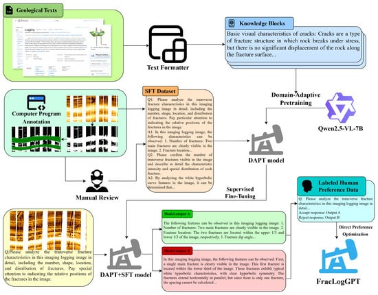
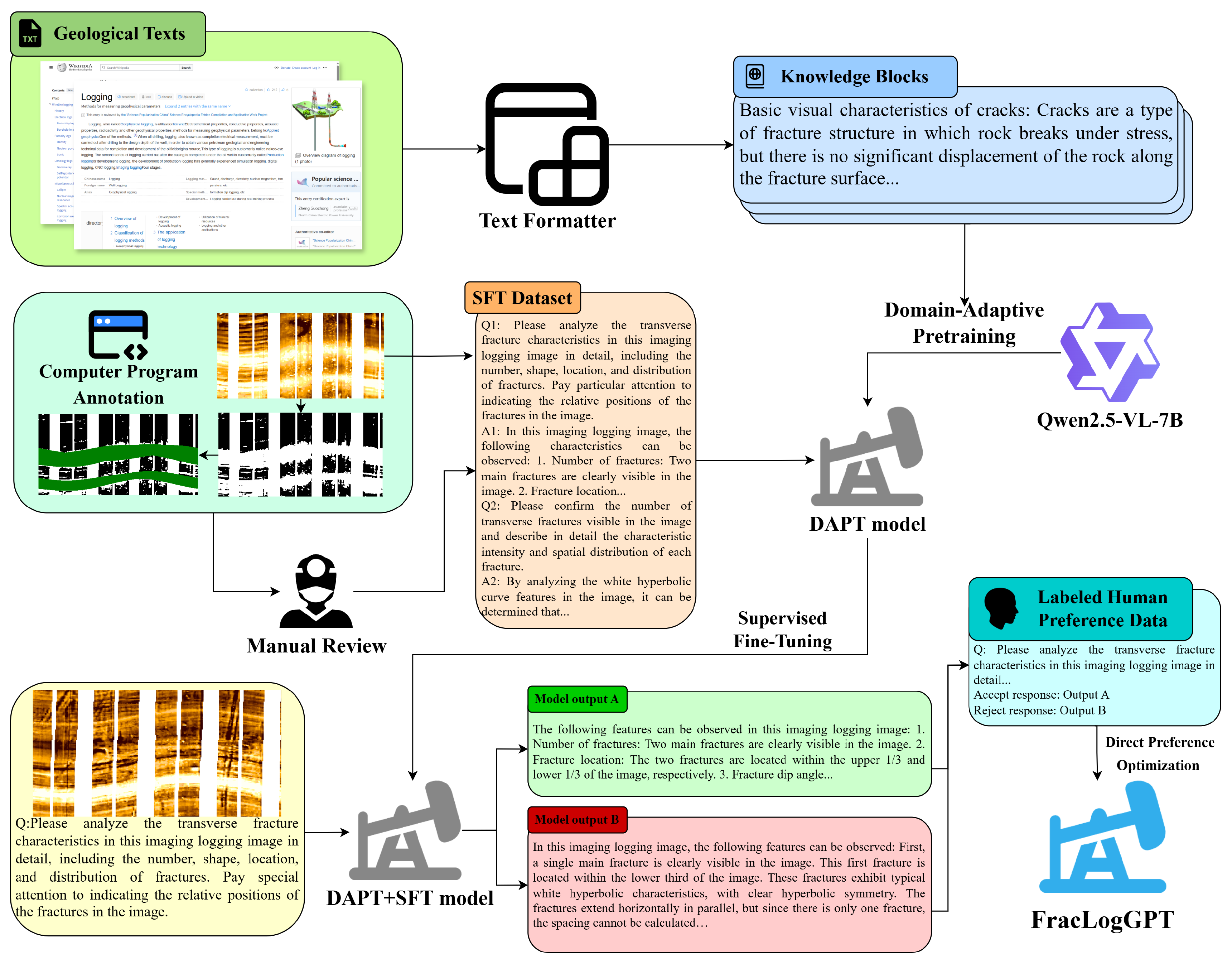
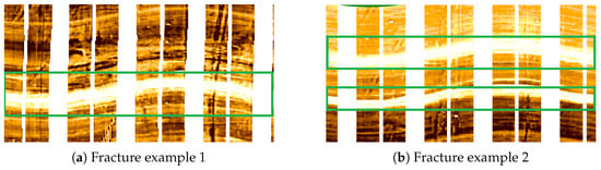
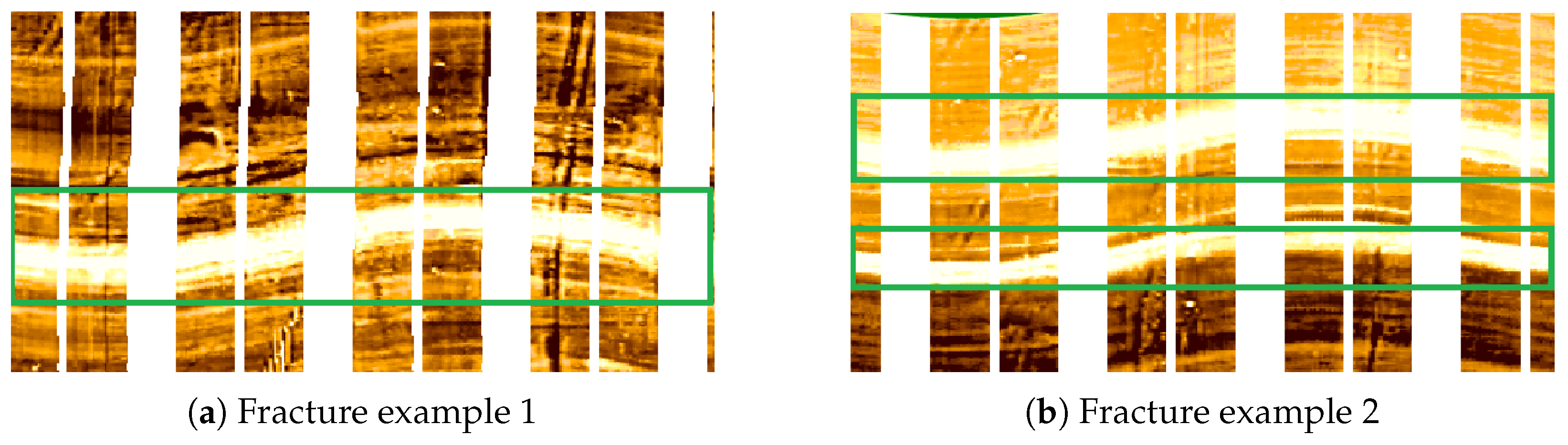
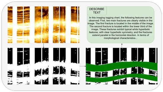
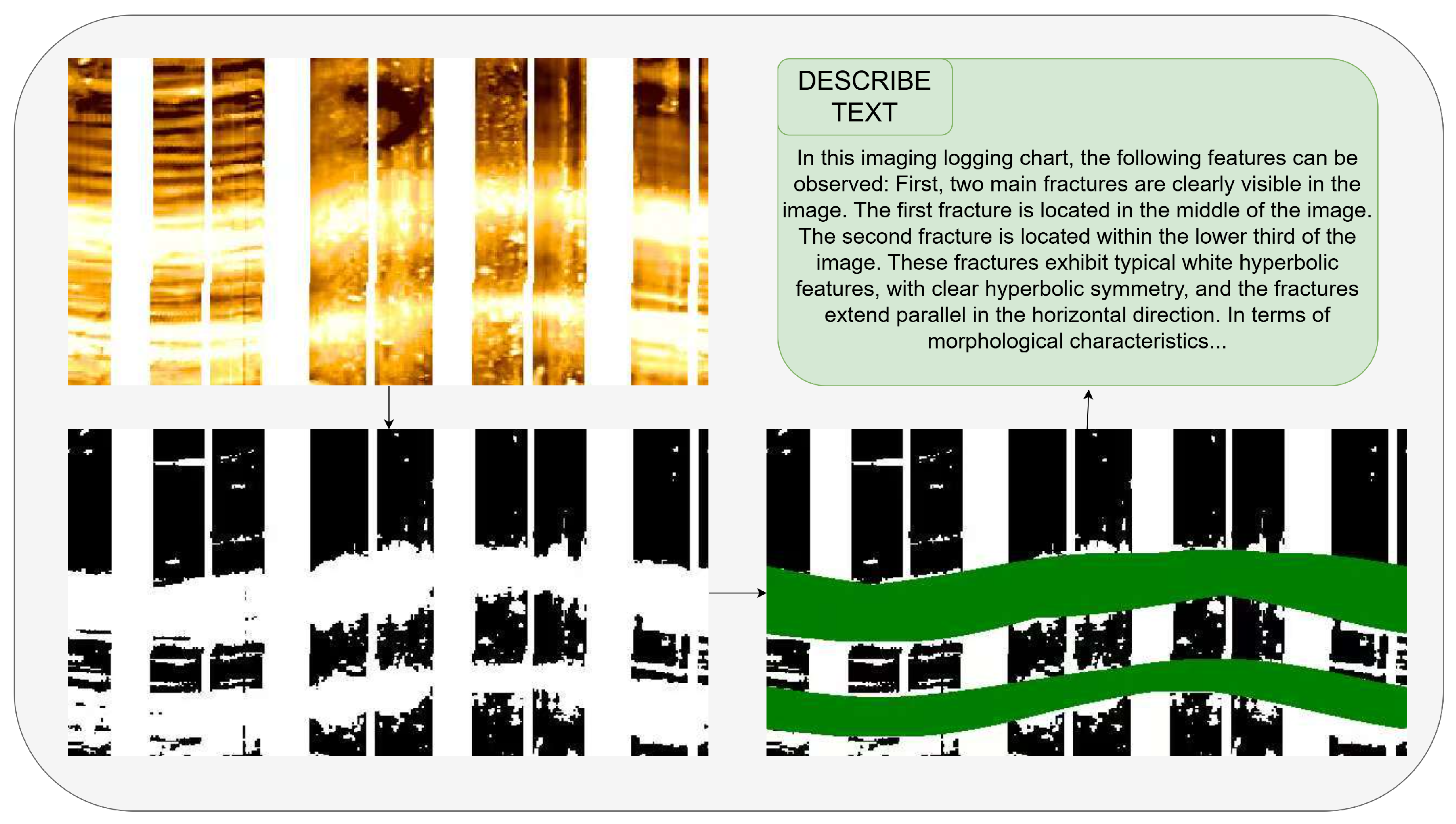
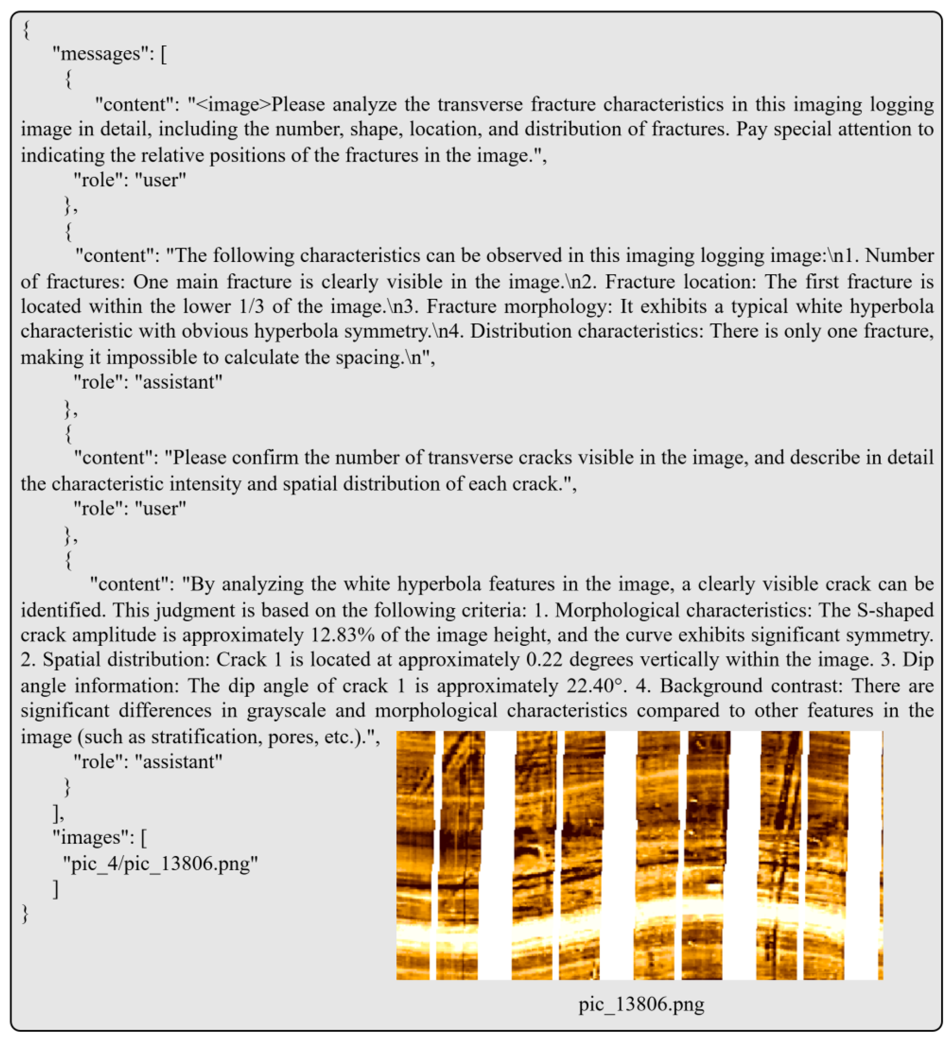
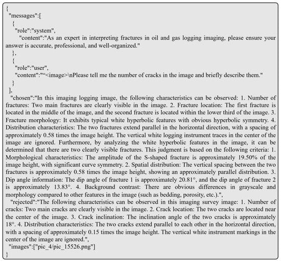
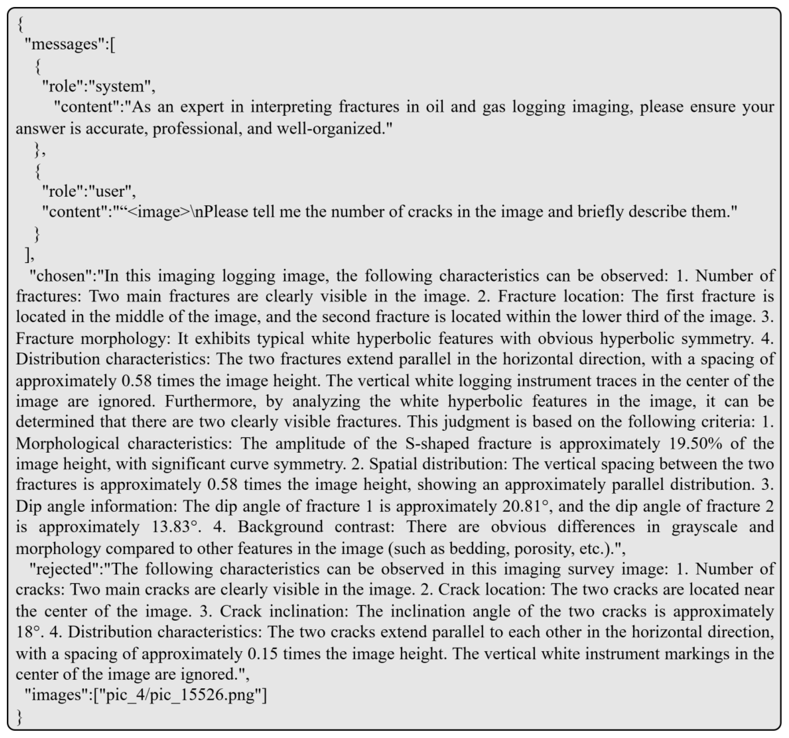
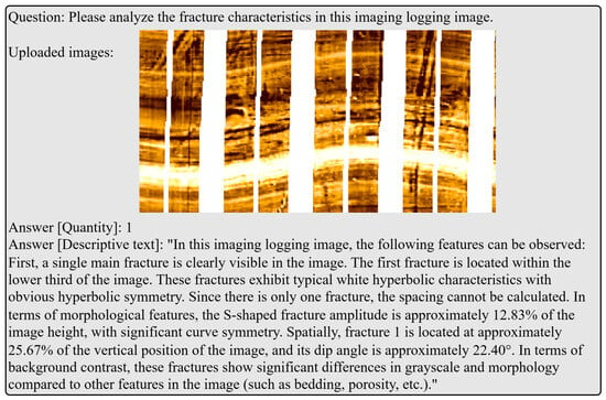
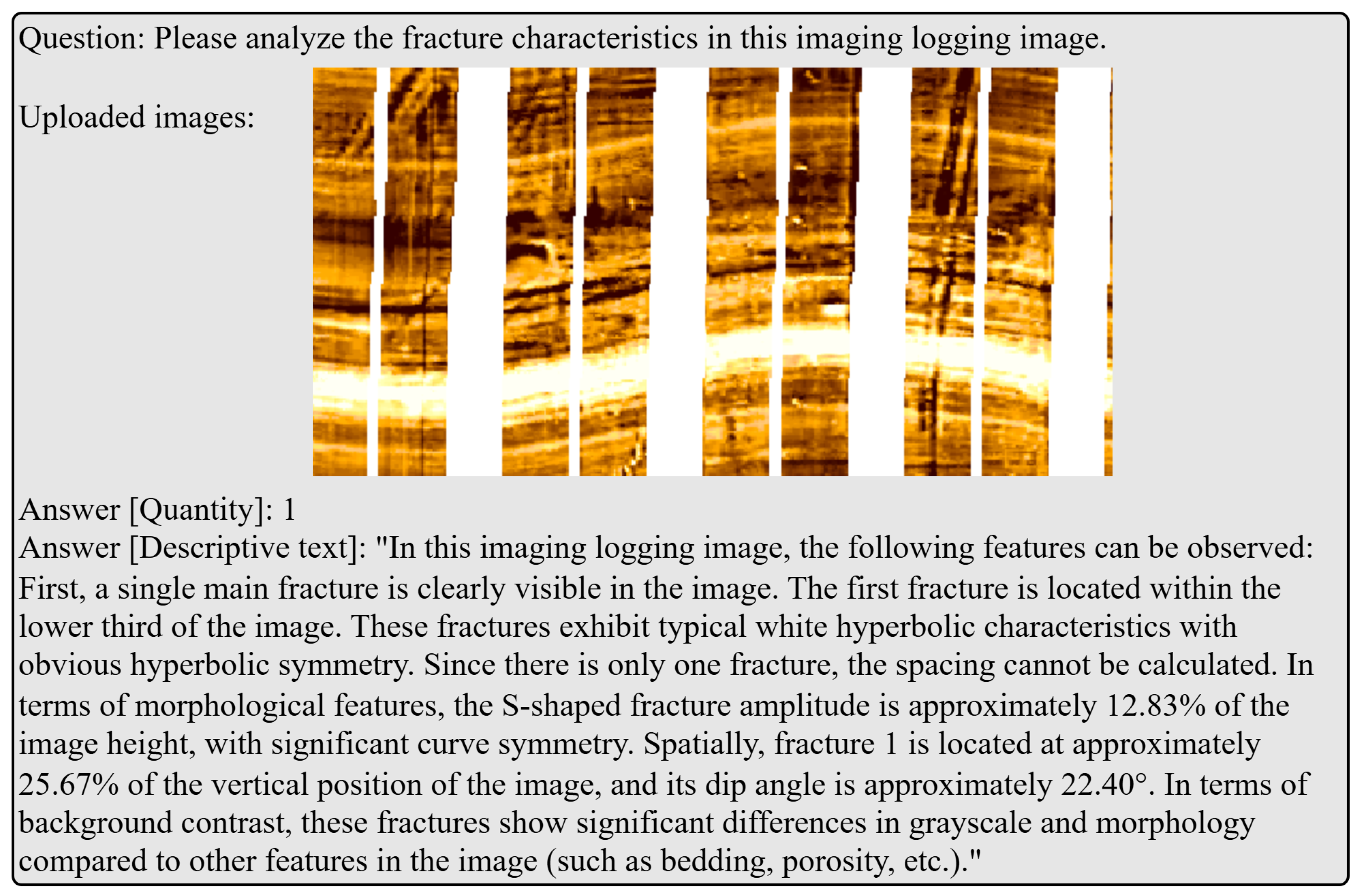

Disclaimer/Publisher’s Note: The statements, opinions and data contained in all publications are solely those of the individual author(s) and contributor(s) and not of MDPI and/or the editor(s). MDPI and/or the editor(s) disclaim responsibility for any injury to people or property resulting from any ideas, methods, instructions or products referred to in the content. |
© 2025 by the authors. Licensee MDPI, Basel, Switzerland. This article is an open access article distributed under the terms and conditions of the Creative Commons Attribution (CC BY) license.