


Abstract
This paper proposes a novel framework that integrates Deep Learning Neural Networks into the Stochastic Parameterized Expectations Algorithm (DLNN-PEA) to solve nonlinear rational expectations models. This method enhances traditional PEA-based solvers by employing a deep neural expectations operator that captures complex nonlinearities and asymmetries. The DLNN-PEA is implemented in Matlab R2024b. It combines deep learning approximation with the standard expectation-iteration structure of the PEA, replacing the conventional shallow ANN-based operator with a deeper architecture that improves both accuracy and stability. The methodology is applied to the stochastic Neoclassical Growth Model, where the DLNN-PEA is trained to approximate conditional expectations and decision rules under uncertainty. The results show rapid convergence, reduced boundary-related issues, and stable performance even in high-volatility environments. Compared with ANN-PEA, deep architectures exhibit greater robustness and adaptability, making them suitable for economic models characterized by stronger nonlinearities and richer state dynamics. Beyond the benchmark model, the proposed framework is well-suited for medium-scale DSGE models, nonlinear monetary policy environments, and macro-financial simulations involving high-dimensional state spaces. These features make DLNN-PEA a practical tool for applied macroeconomic analysis and model-based policy evaluation.
1. Introduction
Despite the remarkable progress in the development of numerical methods over the past decades, solving or estimating nonlinear rational expectations problems continues to represent a major challenge for macroeconomics. This difficulty becomes even more critical when moving from highly theoretical constructs to models intended for policy analysis. The use of neural networks for solving rational-expectations models is a relatively recent development, with early contributions from a few authors [1,2]. Breakthroughs in machine learning have drawn increasing attention to the potential of employing such techniques in macroeconomic problems under rational expectations [3]. Local approximation methods based on perturbation, such as those proposed by Schmitt-Grohé and Uribe (2004), have gained widespread application in policy analysis [4]. The limitations of these approaches in handling complex features, such as occasionally binding constraints, discrete shocks, heterogeneity across agents, asymmetries, and highly nonlinear functions, have motivated continued interest in implementing global solution methods [5].
The rapid advancement of machine learning and artificial intelligence has reinforced this trend, with numerous applications emerging in quantitative macroeconomics. Some authors formulated a continuous-time economic model and employed neural networks to approximate the Bellman equation [6]. Other researchers extended the use of neural networks to approximate equilibrium conditions in heterogeneous-agent models, relying on simulated data for training [7]. A similar perspective was adopted in other research for solving a life-cycle model with borrowing constraints, aggregate shocks, and financial frictions [8]. Additionally, previous research has employed deep neural networks to approximate aggregate laws of motion in a heterogeneous agent setting characterized by strong nonlinearities and shocks [9]. Recently, some researchers have applied neural networks to a New Keynesian three-equation model with a nonlinear Taylor rule [10]. In contrast, others have used machine learning techniques to derive the optimal policy plan in a linear-quadratic version of the Calvo model [11].
Recent advances in machine learning have introduced a wide range of tools for solving nonlinear dynamic economic models, including deep neural networks for policy and value function approximation, reinforcement-learning approaches to forward-looking environments, and neural-network-based expectations operators capable of capturing highly nonlinear conditional distributions. Within this expanding literature, the present paper is positioned within the PEA-based family of methods: rather than constructing an end-to-end learning system, we enhance the expectations operator itself by replacing a shallow ANN with a deep architecture. This alignment ensures methodological comparability while allowing the DLNN-PEA approach to benefit from recent developments in deep learning applied to economic dynamics.
Global numerical methods such as value function iteration, policy function iteration, the endogenous grid-point method, or projection techniques generally require discretization using grids. When applied to large-scale models with multiple state variables, the computational burden grows rapidly. By contrast, the Parameterized Expectations Algorithm (PEA), introduced by Marcet (1988) and further developed by den Haan and Marcet (1990), offers a grid-free global solution method that is more efficient in handling higher-dimensional models [12,13]. Unlike grid-based methods, the stochastic version of PEA simulates the economy along equilibrium-consistent trajectories, computing solutions only for states within the ergodic set.
The efficacy of artificial neural network (ANN)-based models makes them particularly well-suited for application in relatively straightforward environments, as exemplified by the stochastic Neoclassical Growth model. However, even within these contexts, applying PEA may face challenges related to convergence. Research has shown that PEA does not satisfy the properties of a contraction mapping, raising concerns that a solution may not always be guaranteed [14]. To address this limitation, the authors advocate implementing moving bounds to stabilize. ANN-PEA provides a flexible, computationally efficient approach to solving rational expectations models by approximating the conditional expectation embedded in the Euler equation with a shallow neural network. In this framework, the expectation operator is parameterized by a small set of neural network weights, which are iteratively updated until the Euler equation residuals converge. ANN-PEA has proved effective in low-dimensional settings and is widely used as a benchmark due to its speed, simplicity, and stability.
In this context, an approach that integrates DLNN-PEA has been developed for addressing macro-financial models. Building on the work of other authors [15,16] that employed artificial neural networks, the present framework incorporates more advanced deep learning structures to solve nonlinear rational expectations models. Applications to the stochastic Neoclassical Growth model illustrate the potential of this method [17]. The findings suggest that the deep learning design can alleviate issues related to bounds, echoing earlier observations [14]. Moreover, the improved DLNN architecture appears to provide comparative advantages when applied to models with complex rational expectations, significant asymmetries, and pronounced nonlinear dynamics.
This paper focuses on a specific subset of numerical approaches for the PEA family of rational expectations models. The decision to exclusively compare DLNN-PEA with ANN-PEA stems from a deliberate methodological alignment: both methods share the same foundational structure, differing only in the functional form of their expectation operators. This allows for an assessment within a consistent modeling framework, ensuring a controlled and transparent evaluation of the incremental benefits gained by substituting a shallow neural network with a deep architecture [15]. In contrast, comparing DLNN-PEA to solution methods based on fundamentally different principles would not enable a direct, like-for-like comparison of how the depth of the expectations operator influences accuracy, stability, and computational performance.
This study contributes to existing literature by integrating DLNN-PEA to resolve nonlinear rational expectations models. The proposed framework effectively addresses well-documented convergence and stability challenges associated with traditional PEA methods. Additionally, it extends the flexibility of ANN-based approaches by leveraging the expressive power of deeper architectures. To empirically validate this methodology, the research applies it to the stochastic Neoclassical Growth Model, utilizing both benchmark and Romania-based calibrations. A particular focus is placed on the influence of the risk aversion parameter on equilibrium dynamics. Through a comparative analysis of DLNN-PEA, polynomial PEA, and ANN-PEA, this paper delineates the advantages of the proposed algorithm in terms of accuracy, robustness, and computational efficiency.
The rest of the paper is structured as follows. Section 2 presents the macroeconomic framework, derives the Euler equation, and provides a detailed description of the DLNN-PEA, including data transformations, architecture, and training procedures. Section 3 reports the calibration and results, including benchmark exercises, comparisons between ANN-PEA and DLNN-PEA, and counterfactual risk-aversion experiments. Section 4 discusses the implications and future research directions, and Section 5 concludes the findings.
2. Theoretical Framework
The empirical foundation of this study is built upon the stochastic neoclassical growth model, which has become a benchmark in macroeconomic research due to its analytical clarity and broad applicability. This context describes the behavior of a representative household that maximizes expected lifetime utility under an intertemporal budget constraint, with output generated by a Cobb–Douglas production function [18,19]. Productivity shocks are modeled as an autoregressive AR(1) process, which introduces uncertainty and nonlinearity into the system, rendering analytical solutions infeasible. The model thus provides an ideal testbed for evaluating numerical algorithms of PEA and its extensions [20,21].
2.1. The Macroeconomic Framework
The macroeconomic framework considered in this paper is a standard optimal stochastic growth model. In the proposed model, a representative household, acting as a social planner, faces the following optimization problem:
The initial relation (Equation (1)) presented encapsulates the isoelastic utility function as utilized by the representative household, where is the subjective discount factor and σ is the risk aversion parameter, while denotes the expectation operator at time 0. According to this relation, by choosing, from the initial period onward, a sequence of present consumption of non-durable goods and services, as well as a sequence of one-period-ahead capital the representative household aims to maximize the expected lifetime utility subject to the budget constraint specified in (Equation (2)). According to the budget constraint, the representative household allocates resources on current consumption of non-durable goods and services , and on investments in future capital . In the planner’s problem, prices do not play a role as the planner directly determines the allocations. In contrast, in a decentralized equilibrium, prices emerge endogenously to coordinate the actions of different agents and ensure market clearing.
Given the previous two mentions, the expenditure side of the budget constraint is covered by the production of goods and services , respectively, by the remaining capital after a depreciation , has occurred. The production function depicted in Equation (3) adheres to the standard Cobb–Douglas form, incorporating a singular input for capital, where denotes the share of capital in the final output is delineated.
The model considered here is subjected to deviations from its deterministic steady state due to an unexpected shock to total factor productivity technology, defined as a standard AR(1) stochastic process according to Equation (4), where is the auto-regressive coefficient, while is an independent and identically distributed (i.i.d.) innovation, normally distributed with zero mean and variances denoted by .
A variety of approaches can be employed to address the optimization problem at hand. This analysis adopts the current-value Lagrangian formulation, which necessitates the inclusion of the discount factor within the budget constraint (Equation (5)). Accordingly, the current-value Lagrangian is articulated as follows:
The optimal program is defined by the first-order conditions (FOCs) obtained for consumption , future capital and the shadow cost (Lagrange multiplier) related to the budget constraint (Equations (6)–(8)).
The model is fully specified, and the optimal solution is determined by imposing the transversality condition (Equation (9)):
By replacing the Lagrange multiplier (Equation (7)) with marginal utility (Equation (6)), the resulting formulation yields the following Euler relation (Equation (10)):
The expression above basically equates the marginal utility (or welfare benefits) of consumption across two consecutive periods.
Economically, the Euler equation captures the representative household’s intertemporal consumption–savings trade-off. The discount factor β reflects intertemporal patience and determines the weight placed on future utility relative to present utility. The risk-aversion parameter σ governs the curvature of the utility function, influencing consumption smoothing and responsiveness to future uncertainty. Productivity shocks affect the marginal product of capital, thereby shaping incentives for investment. In this sense, the DLNN-PEA does not estimate these parameters but learns the functional relationship implied by the Euler condition and mapping states (capital, productivity) into optimal current consumption.
2.2. Parameterized Expectations Algorithm Approach
PEA approximates the expectations of economic agents in a macroeconomic model using smooth functions [14,20]. Specifically, the algorithm proposed by the promoter authors represents a generalized method of undetermined coefficients, in which the decision rules are determined at each step based on a learning-type mechanism [12,13]. According to Schmitt-Grohé and Uribe [4], the complete set of equilibrium conditions can be expressed as a system of (conditional) expectations in Equation (11):
where is a vector of control variables and represents a vector of state variables, with being a function. The vector of state variables has two blocks: a block of predetermined variables (endogenous state variables) and a block of shocks (exogenous state variables). Equation (11) can be re-expressed as follows:
where defines the model, while denotes a transformation that can be used further to make expectations. Given the macroeconomic model, the expectation articulated in Equation (10) can be formulated with reference to Equation (12) in Equation (13):
Furthermore, the definition of in terms of as follows:
The PEA supposes to find an approximation function (polynomial) of the current state of variables, where denotes a vector of the function’s parameters, in order to replace the transformed expectations such that:
Therefore, the main idea behind the PEA is to find a vector of parameters such that:
where is a small random number. The convergence properties of the PEA are supported by the Weierstrass Approximation Theorem, which states that polynomials can uniformly approximate any continuous function on a compact set [22,23]. More exactly, the class of polynomials is dense in the space of continuous functions, which justifies the use of polynomial or other smooth functional forms in approximating the conditional expectation within the algorithm [24].
For illustrative purposes, one might consider a scenario in which a particular function is expressed as an exponential function of a polynomial. This leads to the formulation of a regression model designed to extract the associated vector. Such an approach further reinforces the applicability of polynomial functions in the context of regression analysis and approximation techniques. then to consider a regression of the form to recover the vector :
The vector will be further refined through the application of a convex dampening scheme. This approach facilitates the construction of sequences for both the endogenous state variables and the control variables, specifically denoted as , , and .
While general formal proof of convergence for deep learning-based expectation operators is not currently available, the DLNN-PEA inherits several desirable convergence properties from the traditional PEA framework. Convergence of the expectation iteration is expected under standard assumptions widely used in the literature:
- The state space is compact, and the simulation remains within the ergodic set;
- The policy functions and conditional expectations are bounded;
- The mapping defined by the Euler equation is Lipschitz continuous;
- The learning update satisfies a contraction property when expectations are evaluated over the ergodic region.
The role of the DLNN is to approximate a smooth conditional expectation operator that preserves these properties. The use of ReLU-based deep architecture ensures universal approximation on compact sets, while regularization and normalization maintain boundedness of the network output. Under these conditions, the DLNN-PEA update behaves like a local contraction, and the sequence of expectation approximations converges to a stable fixed point.
Although complete global proof remains an open question in the machine-learning literature, these assumptions provide a theoretical basis for the empirical convergence observed in numerical experiments and align with the convergence arguments used in related approaches such as ANN-PEA and projection-based methods.
2.3. Overview of Artificial Neural Networks and Deep Learning Neural Networks
The research presents a concise overview of artificial neural networks and deep learning neural networks. Consider a scalar of interest, denoted as y, along with a vector of predictors represented as X. The objective is to approximate or forecast the value of y. To achieve this, a model is employed that is defined as a combination of generalized linear models:
where represents a nonlinear activation function, and W are weights assigned to the predictors, with and . In fact, the function above corresponds to a perception performing forward propagation. It can also be expressed as a summation representing the linear combination of its inputs:
Furthermore, hidden layers can be introduced between the inputs and the final output to construct an artificial neural network (ANN) :
The integration of multiple layers within an ANN facilitates the establishment of a DNN system. This system is characterized by an architecture that enables the modeling of complex patterns through hierarchical processing of information, defined as follows:
The aforementioned mathematical construction exhibits a feedforward structure akin to a directed acyclic graph. In this sense, the goal of a data scientist or an economist is to find the weights w such that the estimated fitted to be as close as possible to the realized y. Evaluating such a fit involves considering an appropriate metric, such as the norm, for example. The learning feature for the neural networks defined above is based on a backpropagation approach to determine optimal weights w. Accordingly, the following loss function will be defined:
where I denote the length of vectors.
The objective is to identify the weights that effectively minimize the designated loss function. In the context of a deep neural network architecture, each hidden layer is associated with distinct weights. The backpropagation methodology is employed after an initial assessment of the loss function, facilitating the process of updating the weights in a backward manner to minimize the loss function. A widely adopted algorithm for this optimization task is stochastic gradient descent. Moreover, the activation function can manifest in various forms. Typically, for hidden layers, the activation function is defined based on the Rectified Linear Unit (ReLU) activation function:
where z denotes a hidden layer.
For the output layer, the activation function is defined based on the sigmoidal function:
or on the SoftMax function:
To transition from ANN-PEA to DLNN-PEA, the process adheres closely to the algorithm presented by Valaitis and Villa [15], with the distinction that ANN-based expectations are substituted with DLNN. Furthermore, in contrast with that research, two normalization steps are implemented, which will be elaborated on later in the algorithm description. Normalization is a standard technique, particularly for Deep Learning models applied to time series data that may exhibit variations in scale, as it contributes to stabilizing training and accelerating convergence. Consequently, the DLNN-PEA encompasses the following steps:
- ⚬
- Step 1: Simulate a log AR(1) time series for technology shocks with T = 5000:
- ⚬
- Step 2: The AR(1) series for is fed into the steady-state relation for capital, and then obtain steady-stated based initial consumption, respectively, the initial right side of the Euler equation as (SSRS):
- ⚬
- Step 3: Transforming the data as follows: normalizing the state variables and min-max scaling for
- ⚬
- Step 4: Defining a model of DLNN
- ⚬
- Step 5: Training the DLNN model on the training set obtained in step 3, which means that:where denote the operator of unconditional expectation, while error > then
- ⚬
- Step 6:For t = 1: Tif t = 1 then DLNN =else DLNN from the last training
- ⚬
- Step 6.1: Using the last trained DLNN predict the scaled by using the normalized
- ⚬
- Step 6.2: Getting from step 6.1, to rescale as:
- ⚬
- Step 6.3: Obtain as following:
- ⚬
- Step 6.4: Using from the previous step, the one-ahead capital was determined:
- ⚬
- Step 7: Calculate the new right side of the Euler equation as:
- ⚬
- Step 8: Transforming the data as following: normalizing the state variables and and min-max scalling for
- ⚬
- Step 9: Training the DLNN model on the training set obtained at the previous step
- ⚬
- Step 10: Computing the error:
- ⚬
- Step 11: Checking the convergence and updating the sequence for capital: if then will be in the next iteration else stop the algorithm.
3. Results
The proposed deep learning model is a fully connected feedforward neural network designed for regression tasks. The architecture begins with an input layer that receives two explanatory variables (the number of state variables), followed by three hidden layers with 32, and 16 neurons, respectively. Each hidden layer is activated using the ReLU function to capture nonlinear relationships (Table 1).
Table 1.
Deep Learning Network Architecture.
The DLNN-PEA framework employs a deep neural architecture composed of three fully connected layers, with 64, 32, and 16 neurons, respectively. Each layer uses the ReLU activation function, which facilitates faster convergence and mitigates the vanishing gradient problem common in deep networks. The network is trained to approximate the conditional expectations embedded in the model’s equilibrium conditions, using a Half Mean Squared Error (HMSE) loss function that penalizes large deviations symmetrically while maintaining numerical stability. Training is conducted for up to 50 epochs with mini-batches of 250 observations, ensuring efficient gradient updates and smooth convergence.
The 64-32-16 architecture was selected after a series of preliminary experiments balancing accuracy, convergence speed, and computational cost. Shallow networks tended to underfit, failing to capture the nonlinearities of the conditional expectation operator, while substantially deeper networks provided only marginal accuracy improvements at significantly higher computational cost. The architecture used in this study, therefore, reflects a compromise between expressive power and efficiency. Moreover, the monotonic decline in the RMSE and Loss values indicates that this configuration achieves stable convergence, supporting its suitability for the benchmark model’s dimensionality.
Model regularization is achieved through L2 weight decay with a coefficient of 0.001, limiting overfitting and improving generalization across simulated states of the macro-financial model. The learning process is optimized using the ADAM algorithm, with a base learning rate of 0.001 and a validation frequency of 950 iterations. This configuration balances computational efficiency and accuracy, allowing the DLNN-PEA to capture complex nonlinear relationships between state variables and expected future outcomes. To complement this architectural description, Table 2 provides quantitative performance indicators (RMSE, convergence speed, and computation time) for both DLNN-PEA and ANN-PEA. These metrics illustrate how the optimization choices described above translate into practical numerical gains.
Table 2.
Quantitative Comparison of ANN-PEA and DLNN-PEA Performance.
In addition to the direct timing and memory indicators, the DLNN-PEA exhibits favorable scalability properties. Because the algorithm avoids grid-based discretization, its computational burden does not grow exponentially with the number of state variables. Instead, increases in dimensionality mainly affect the size of the input layer and the corresponding weight matrices, leading to approximately linear growth in computation time. This makes the DLNN-PEA suitable for medium- and high-dimensional macro-financial models where traditional global solution methods become computationally infeasible.
Table 3 presents the results for the annually calibrated model. The benchmark calibration employs commonly accepted parameters to examine various aspects of the stochastic neoclassical growth model and the Real Business Cycle (RBC) model. This calibration aligns closely with the characteristics of the U.S. economy, thereby ensuring that the parameters are representative of a mature economic environment.
Table 3.
Parameter calibration for the stochastic Neoclassical growth model.
Alternatively, the model may be calibrated to reflect conditions pertinent to the Romanian economy. In this context, the parameters exhibit significant deviations from the benchmark, capturing the unique attributes of an emerging economy. Specifically, notable disparities are observed in the capital share in final output and the depreciation rate. Following the framework established by Copaciu et al. [25], the capital share in final output is set at 0.5, and the depreciation rate is set at 4.9% every quarter, yielding an annual depreciation rate of 19.6%. Given the relatively elevated capital-related parameters, the subjective discount factor is correlated with the average yearly interest rate on loans, which stabilized at 6%.
The parameters influencing total factor productivity dynamics are calibrated using empirical estimates, yielding a persistence coefficient of 0.96 and a standard deviation of approximately 1%. In the calibration of the Romanian economy, various values of the risk aversion parameter are examined, with 2.5 deemed the most plausible (Figure 1).
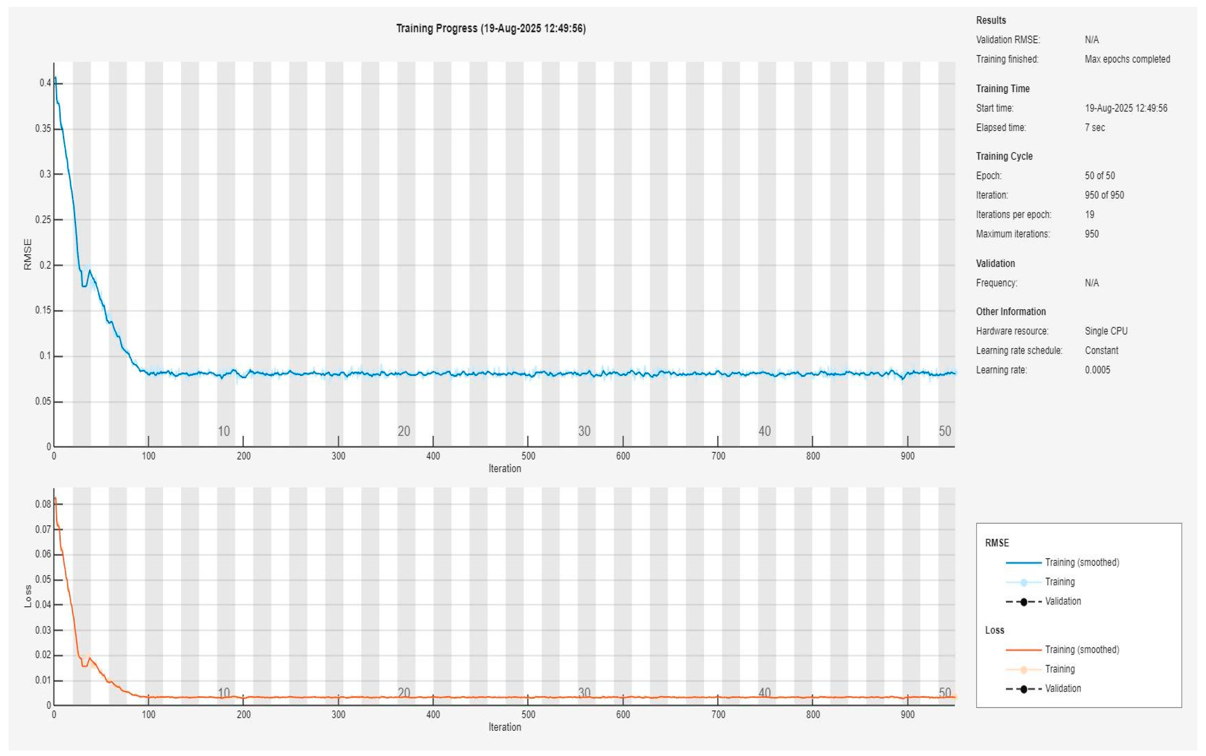
Figure 1.
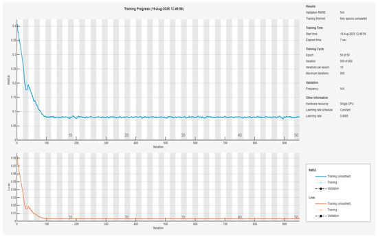
Initial training of the DLNN-PEA for the benchmark calibration.
The two methodologies, ANN-PEA and DLNN-PEA, are analyzed to assess their effectiveness in approximating solutions to the stochastic Neoclassical Growth Model across varying parameter configurations. The initial phase involves implementing a benchmark calibration, in which both approaches are used to estimate the model under rational expectations. An evaluation of the initial training set is presented before the commencement of the iterative loop, specifically corresponding to step 5 of the algorithm delineated in the preceding section. For subsequent counterfactual exercises, only the initial training of the DLNN-PEA, as outlined in step 5, will be reported.
In deep learning, the Root Mean Squared Error (RMSE) is a metric that quantifies the average magnitude of the model’s prediction errors. This statistic provides insight into how closely the predicted values align with the actual values, retaining the original units of the dataset. A lower RMSE signifies enhanced model accuracy. Conversely, loss is the value of the objective function that the model aims to minimize during training. In regression contexts, this is frequently expressed as the mean squared error (MSE) between predicted and actual values, thereby illustrating the extent of deviation in the predictions. A lower loss indicates a better fit to the training data.
An RMSE that stabilizes around 0.08 following the initial 100 iterations suggests that the model has effectively captured a representative understanding of the data. Concurrently, a loss metric below 0.01 reflects a significant decrease in the mean squared error, indicating a robust fit. The training plot is expected to show a rapid decline in the initial epochs, followed by a plateau or minor oscillations as it approaches its final values. The performance of the DLNN-PEA in this context appears satisfactory.
It is important to note that, since the data used within the DLNN-PEA and ANN-PEA procedures are generated directly from the structural model rather than drawn from an empirical sample, the goal is numerical approximation rather than statistical inference. Consequently, confidence intervals that quantify sampling uncertainty in econometric estimation are not applicable in this context. This approach is fully consistent with the existing literature on PEA and machine-learning-based solvers [15,20], where robustness is evaluated through numerical accuracy measures such as RMSE, MSE, and Euler-equation errors rather than interval estimates.
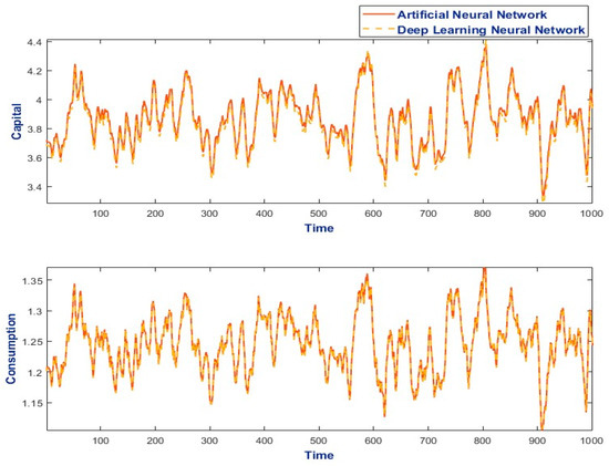
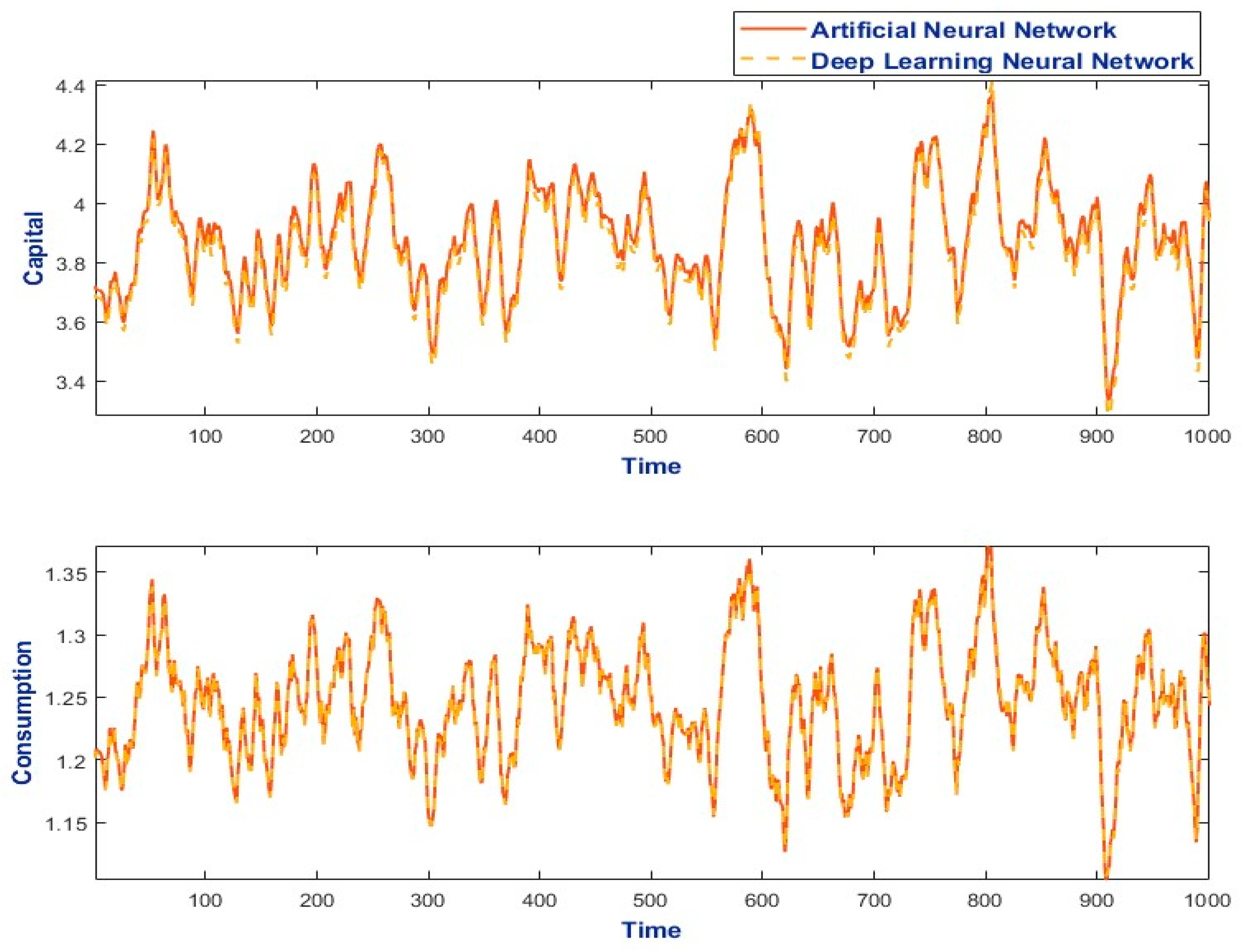
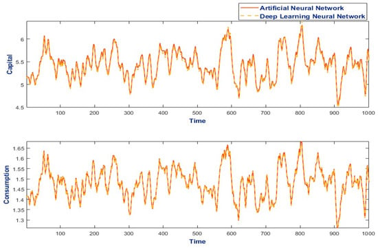
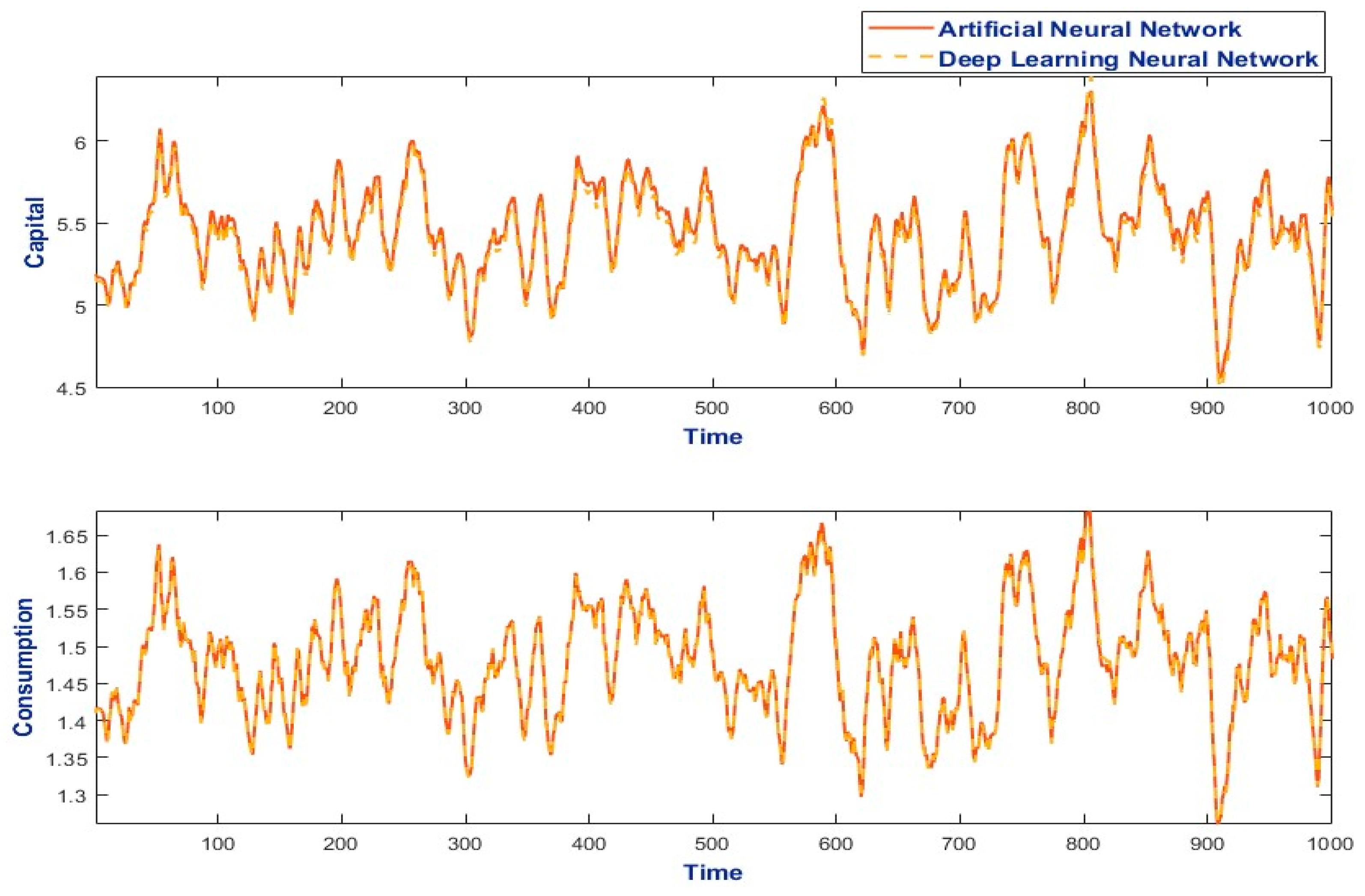
In the preliminary phase, a target convergence tolerance of 2% is established for the DLNN-PEA, specifically for iterations executed in steps 6–11 of the iterative loop. A stricter tolerance of 0.4% is applied to the ANN-PEA. The 2% threshold is deemed a judicious choice for this investigation: the primary aim is to scrutinize the comparative behavior of the DLNN-PEA against that of the ANN-PEA, in addition to deriving a DLNN-PEA solution within a limited number of iterations due to the elevated computational complexity associated with the deep model in comparison to the shallower ANN. The report subsequently includes a simulation depicting the evolution of capital and consumption over a 1000-period horizon, following a 1000-period burn-in. The resulting plots demonstrate that the consumption trajectories produced by both algorithms are nearly indistinguishable (Figure 2).
Figure 2.
Benchmark calibration with error thresholds set to <2% for DLNN-PEA and <0.4% for ANN-PEA.
Figure 2 shows that the consumption paths produced by ANN-PEA and DLNN-PEA almost fully overlap, reflecting the strong consumption-smoothing property implied by the Euler equation. The near-identical trajectories confirm that both algorithms successfully reproduce the household’s optimal intertemporal choice, with DLNN-PEA capturing marginal-utility dynamics slightly more accurately during periods of higher volatility. Differences in the capital series are minimal and primarily observable during periods of elevated volatility. The DLNN-PEA exhibits rapid convergence, achieving an error rate of 1.69%, which falls below the established threshold of 2%, within just 10 iterations. The total computation time for this process is recorded at under 2 min.
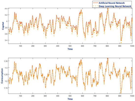
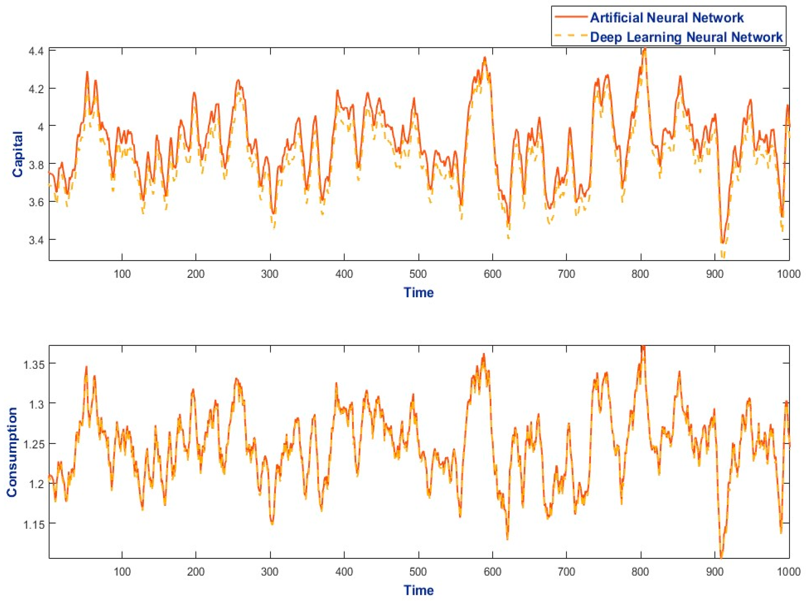
In contrast, applying a 2% threshold to both the DLNN-PEA and ANN-PEA reveals more pronounced disparities in capital evolution after a 1000-period burn-in. Notably, the capital trajectory generated by the ANN-PEA exhibits slightly higher volatility, with its levels predominantly exceeding those observed with the DLNN-PEA (Figure 3).
Figure 3.
Benchmark calibration with error thresholds set to <2% for DLNN-PEA and ANN-PEA.
Figure 3 illustrates that DLNN-PEA generates a smoother capital trajectory than ANN-PEA under the same 2% error threshold. Economically, this reflects the deeper network’s superior ability to approximate the nonlinear mapping from current states to expected future marginal returns, leading to more stable savings decisions and reduced amplification of shocks compared to the shallower ANN-PEA architecture.
Figure 4 shows that, under the Romanian calibration with σ = 1, DLNN-PEA maintains stable, economically coherent trajectories for consumption and capital, whereas ANN-PEA becomes more sensitive to the persistence of the great shock and to a higher capital share. This pattern is consistent with documented boundary issues in shallow networks and highlights DLNN-PEA’s robustness in environments with strong nonlinearities.
Figure 4.
Benchmark calibration only with error thresholds set to <2% for DLNN-PEA and <0.4% ANN-PEA—risk aversion parameter is set to 1.
In Figure 4, the calibration process is conducted exclusively for shocks, while a calibration based on Romanian data is applied to the remaining parameters.
The error thresholds are established at less than 2% for the DLNN-PEA and less than 0.4% for the ANN-PEA.
The subsequent step involved an investigation into the performance of the two models under a calibration specific to the Romanian economy, while maintaining the risk aversion parameter at 1 (Figure 5). In this context, the ANN-PEA produced intricate solutions for capital allocation, necessitating the cessation of iterations. This complication appears to be associated with the boundary problem as discussed by Maliar and Maliar [14] and further analyzed by Valaitis and Villa [15].
Figure 5.
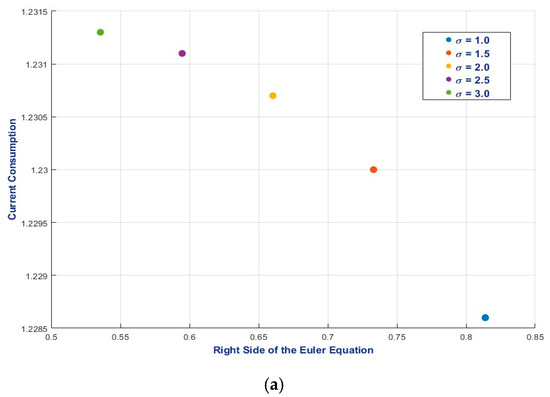
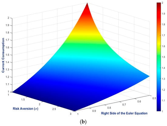
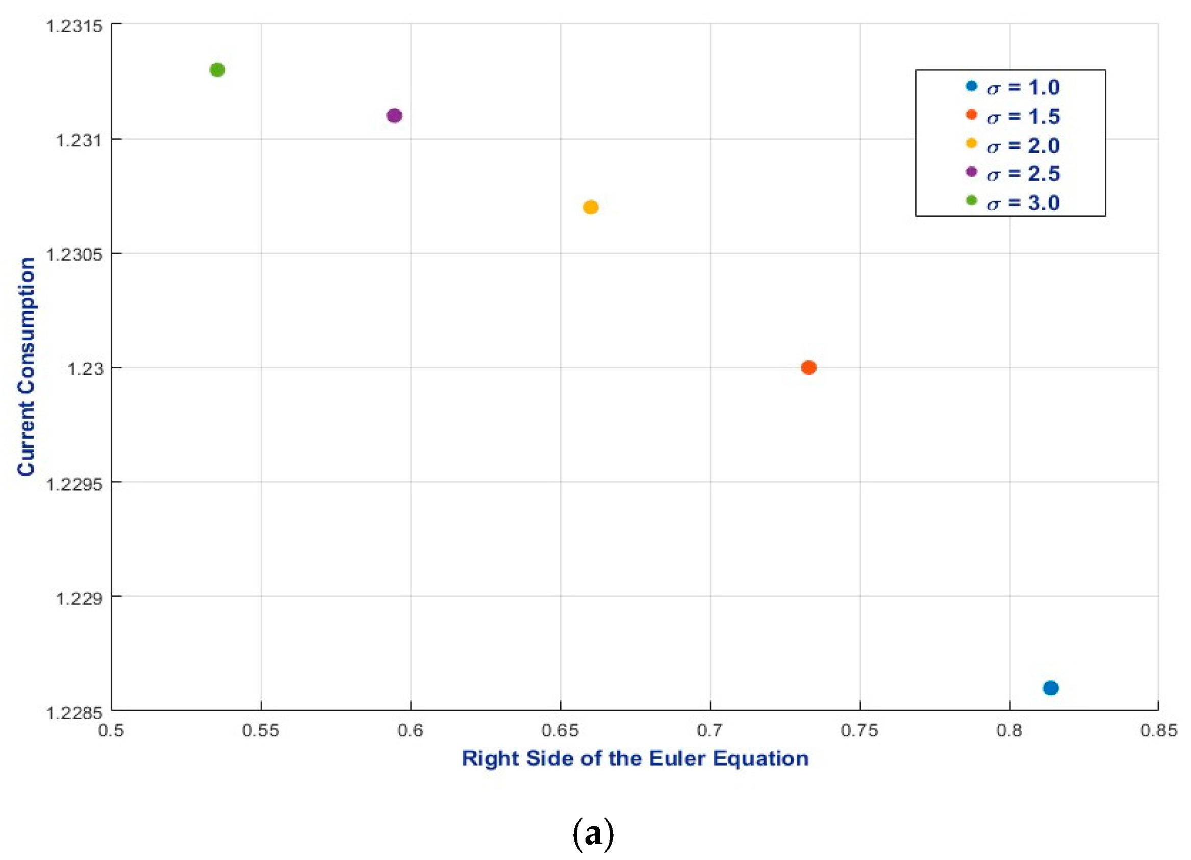
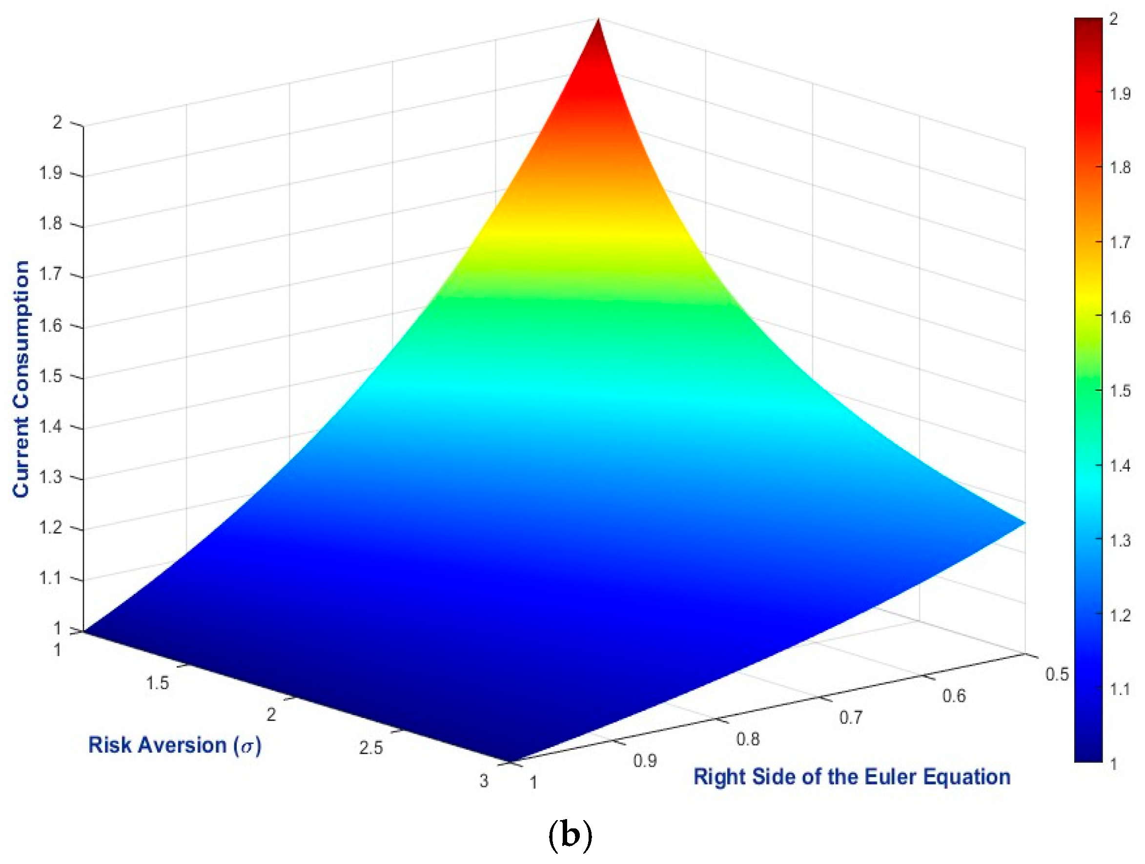
Static and dynamic effects of risk aversion on current consumption and the Euler equation: (a) static effects; (b) dynamic effects.
To mitigate this issue, an alternative approach was implemented: the parameters governing the technology shock dynamics were retained from the benchmark calibration. In contrast, the remaining parameters were calibrated to align with the Romanian economic framework, again with the risk aversion parameter fixed at 1. In this instance, the ANN-PEA achieved convergence, and the comparative analysis with the DLNN-PEA is presented below. Notably, no significant differences were observed in the consumption trajectories generated by the two algorithms. For capital allocation, the paths derived from both methodologies showed remarkable similarity, with only minor discrepancies that are not economically significant.
Figure 5 demonstrates that increasing risk aversion amplifies the responsiveness of consumption and capital to productivity shocks, consistent with a lower elasticity of intertemporal substitution. DLNN-PEA consistently produces smoother and more internally consistent decision rules across all σ scenarios, indicating a more accurate learning of the intertemporal trade-off embedded in the Euler equation.
4. Funding and Discussion
An essential component of the stochastic Neoclassical growth model, as resolved by the PEA, is the risk aversion parameter, which directly influences the Euler equation. As elaborated in the methodological sections, the right-hand side of the Euler equation is approximated using either polynomial functions or neural networks, facilitating the computation of current consumption. Consequently, the risk aversion parameter simultaneously impacts both the right-hand side of the Euler equation and the derived current consumption.
To elucidate this effect, two counterfactual exercises were undertaken through counterfactual calibration. The first exercise evaluated the static implications of the risk aversion parameter by calibrating consumption and capital to their steady-state values while assuming a 2% increase in the technological shock (see the top panel of Figure 5). Six distinct scenarios were analyzed, with the risk aversion parameter ranging from 1 to 3.
The second counterfactual exercise (illustrated in the bottom panel of Figure 5) investigated five risk aversion scenarios in conjunction with variations in the right-hand side of the Euler equation, which was permitted to adopt values between 0.5 and 1. As indicated by the top panel, under certain conditions, variations in the risk aversion parameter may yield minimal impacts on current consumption while eliciting substantial effects on the right-hand side of the Euler equation. Conversely, the bottom panel highlights that low values on the right-hand side may lead to pronounced impacts on current consumption following adjustments to the risk aversion parameter.
These counterfactual analyses suggest that the influence of the risk aversion parameter on decision rules may be nonlinear. Accordingly, the ensuing investigation examines how fluctuations in risk aversion affect solutions derived from the DLNN-PEA, using Romanian-based calibration across the full parameter set. For these assessments, an error threshold of 4% was established. Notably, the steady-state capital under this calibration was nearly twice that under the benchmark calibration. The primary focus of this analysis remains on the behavior of the DLNN-PEA approach, underscoring its rapid convergence to a solution. It is acknowledged that in alternative contexts, enhancing the numerical implementation to refine solution accuracy may be warranted.
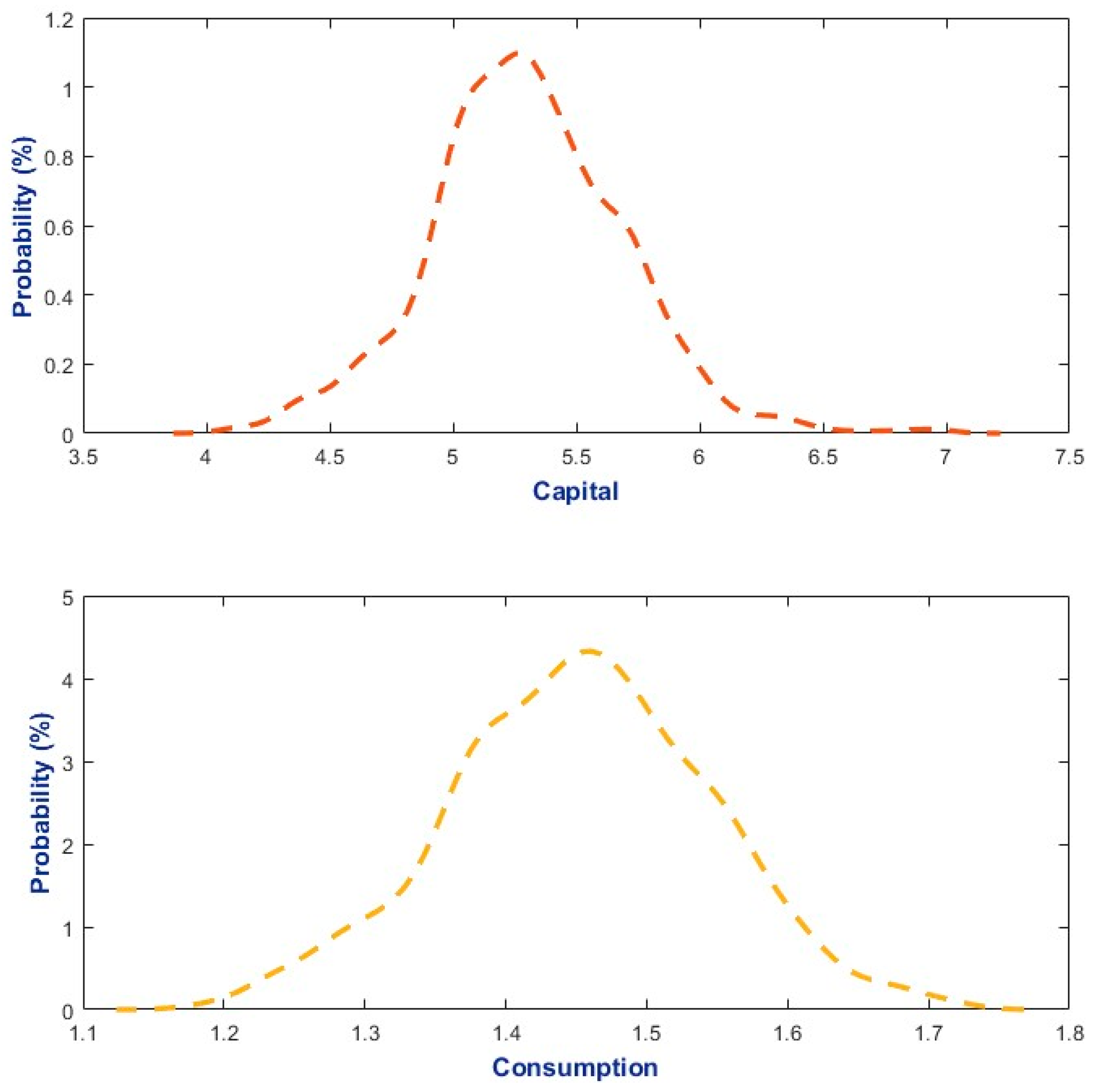
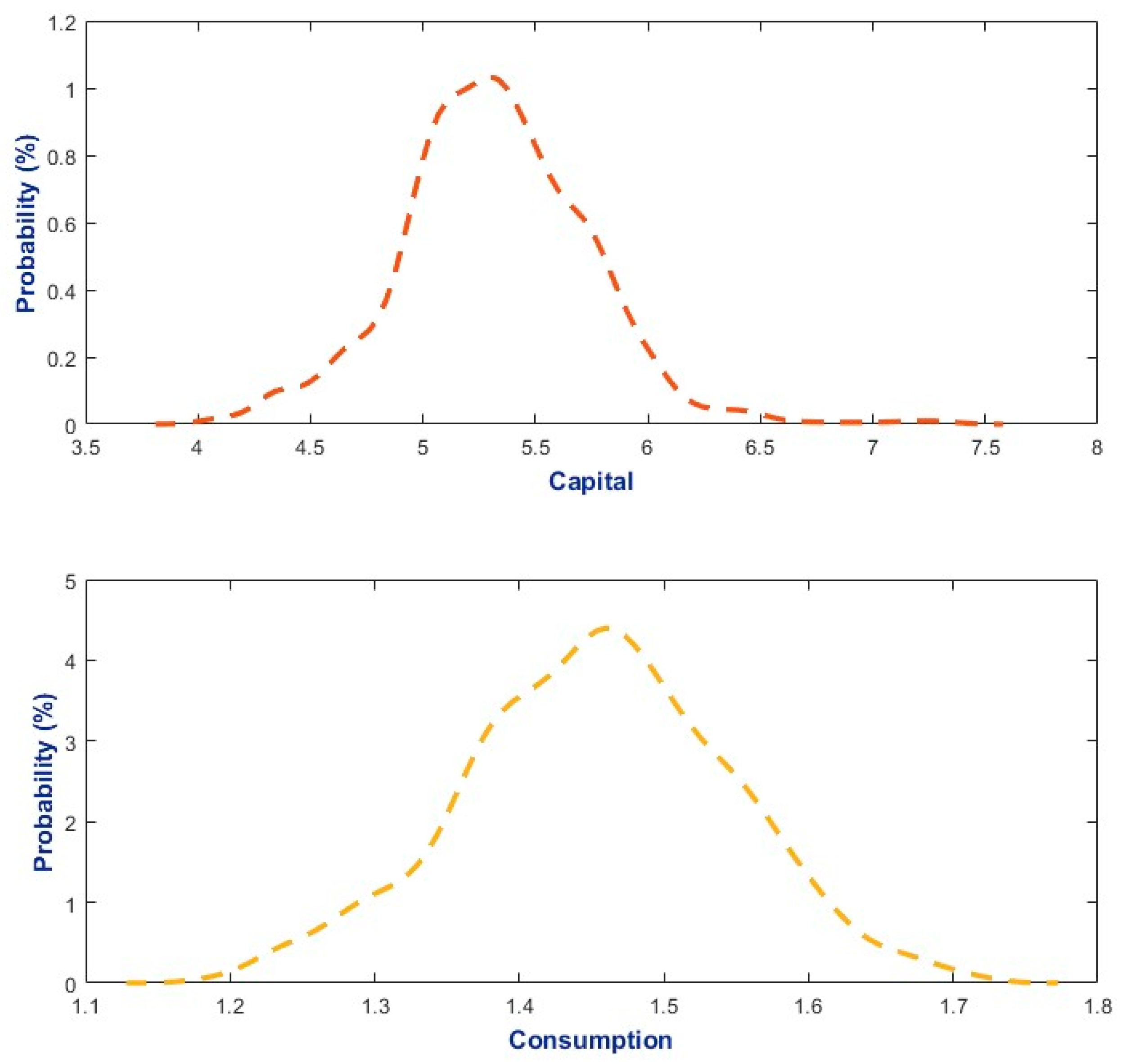
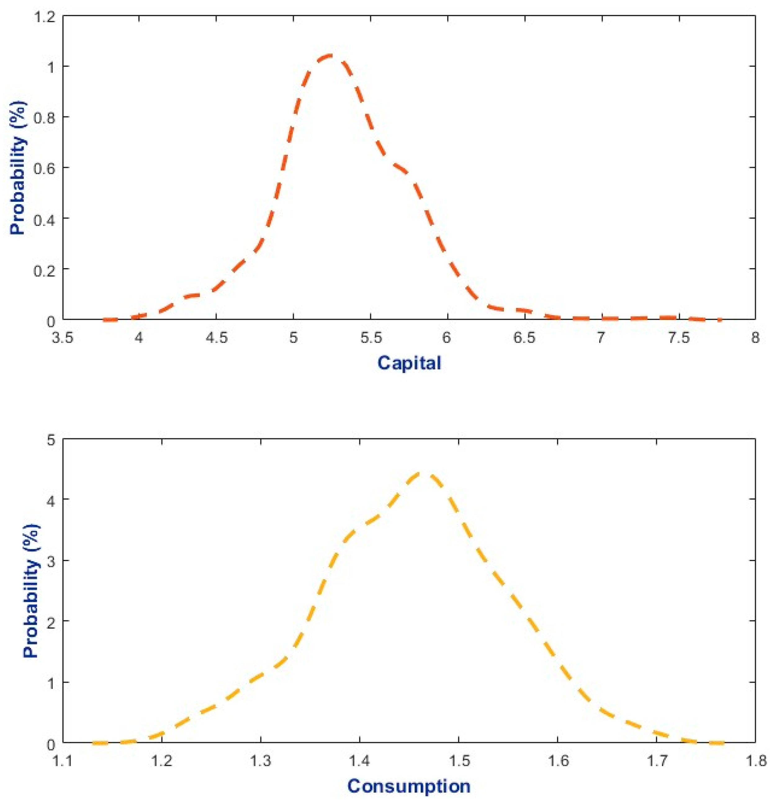
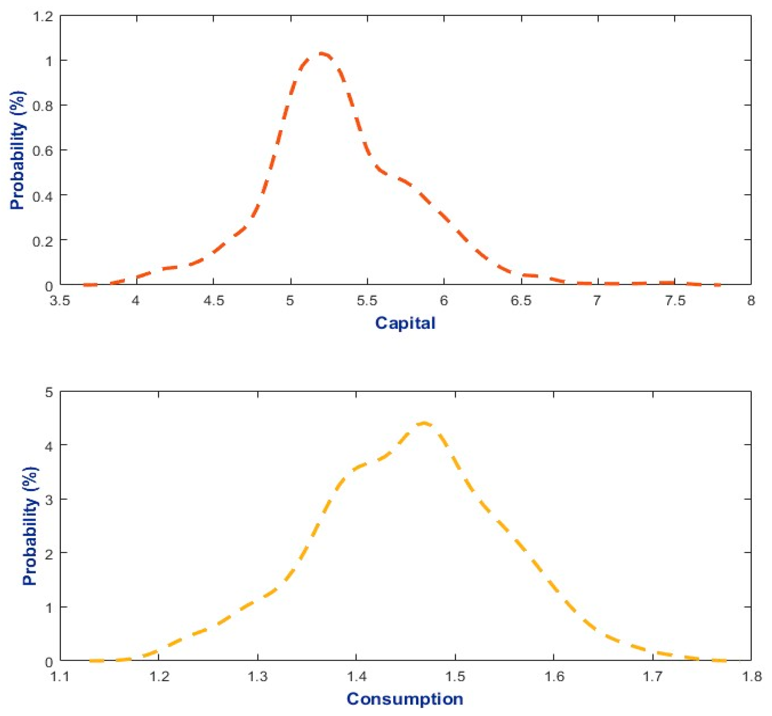
The study examines the implications of altering risk aversion on three dimensions: the DLNN-PEA model evaluation, the decision rules, and the stochastic behavior of consumption and capital, as assessed through empirical density functions. The results, documented in Appendix A, Appendix B, Appendix C and Appendix D, detail these three dimensions across four scenarios, where the risk aversion parameter was sequentially adjusted to values of 1.5, 2, 2.5, and 3. The findings reveal that risk aversion significantly influences both the model’s training and the solutions yielded by the DLNN-PEA, particularly in terms of decision rules and stochastic characteristics. Furthermore, it is noteworthy that the Artificial Neural Network-Policy Evaluation Algorithm (ANN-PEA) failed to converge to a unique solution when the risk aversion parameter exceeded 1, even within the standard calibration.
Moreover, the algorithm effectively accommodates counterfactual scenarios, facilitating an investigation into the impact of variations in key parameters, such as the risk aversion coefficient, on the model’s decision rules and stochastic behavior. The robustness of the DLNN-PEA framework is further validated through its application to alternative calibrations, including a case study centered on the Romanian economy, which underscores its adaptability to diverse economic contexts.
The analysis of risk aversion reveals that its influence on consumption and the Euler equation may exhibit significant nonlinearity. However, DLNN-PEA adeptly captures these effects, whereas ANN-PEA, in contrast, faced convergence challenges under similar conditions or failed to converge. Additionally, the more complex architecture of the DLNN framework may mitigate issues related to bounds.
Although the numerical implementation in this paper is based on the benchmark stochastic Neoclassical Growth Model, the DLNN-PEA framework is not restricted to this environment. The absence of grid-based discretization and the universal approximation capability of deep neural networks make the method suitable for applications with occasionally binding constraints (e.g., borrowing limits, ZLB monetary policy rules), heterogeneous-agent structures, or models featuring multiple equilibria. In such settings, traditional projection or perturbation methods often struggle due to nonlinearity and high dimensionality, whereas the DLNN-PEA can directly approximate conditional expectations over the simulated ergodic distribution. These features highlight the potential of DLNN-PEA to scale to richer DSGE frameworks and policy-relevant macro-financial models.
While the DLNN-PEA method offers several advantages, it also presents important limitations that deserve consideration. Firstly, the use of deep neural networks can lead to overfitting on simulated training trajectories, particularly when the state space is sparsely populated or when the model undergoes extensive training over many epochs. Secondly, the performance of DLNN-PEA is highly sensitive to hyperparameter selection, such as the number of layers, the number of neurons, the learning rate, and the regularization strength, necessitating meticulous tuning to achieve numerical stability. Additionally, like many deep learning architectures, the interpretability of DLNN-PEA is constrained: although the algorithm learns a high-dimensional functional representation of expectations, the network’s internal structure does not transparently elucidate economic mechanisms as polynomial or low-order approximations can. These considerations highlight that, while DLNN-PEA is a formidable numerical tool, its implementation requires careful attention to robustness, diagnostics, and checks for economic plausibility.
The comparative analysis in this study is intentionally restricted to ANN-PEA, following the methodological benchmark [15]. Our contribution focuses on assessing whether deep learning architectures can enhance the traditional PEA framework within an identical modeling setup. A broader comparative evaluation remains an important direction for future research.
5. Conclusions
This study elucidates the efficacy of integrating deep learning neural networks with the stochastic DLNN-PEA methodology for addressing intricate macroeconomic models within the rational expectations framework. By applying this approach to the stochastic Neoclassical Growth model, it is demonstrated that DLNN-PEA achieves rapid convergence and produces stable solutions, even in the presence of nonlinearities that typically challenge traditional methods such as ANN-PEA. The findings indicate that the consumption and capital trajectories generated by DLNN-PEA closely align with benchmark solutions, characterized by reduced volatility in capital dynamics while preserving computational efficiency. Compared with the traditional ANN-PEA benchmark, the DLNN-PEA framework achieves faster convergence, reduced boundary distortions, and higher accuracy in the stochastic Neoclassical Growth Model. These results highlight the theoretical potential of deep learning architectures to strengthen the numerical foundations of PEA-based solvers.
The findings of this study advocate integrating deep learning methodologies into stochastic simulation approaches, as they not only alleviate numerical challenges, such as the curse of dimensionality, but also provide a versatile, scalable solution for high-dimensional, nonlinear macro-financial models. This positions DLNN-PEA as a valuable instrument for quantitative macroeconomics and policy analysis, particularly in scenarios where traditional approximation techniques may be inadequate or demand excessive computational resources. The study lays the groundwork for further exploration of advanced machine learning applications in economic modeling, encompassing cases with heterogeneous agents, occasionally binding constraints, and complex shock structures, thereby underscoring the method’s potential for future research and practical policy implementation.
The DLNN-PEA framework provides several concrete avenues for practical implementation. First, the method can be embedded into medium-scale and large-scale DSGE models where traditional projection or perturbation methods become computationally intensive. Second, DLNN-PEA can be employed in monetary policy analysis by enabling the computation of nonlinear impulse responses, state-dependent policy effects, or optimal policy plans in environments where the Taylor rule or policy constraints exhibit strong asymmetries. Third, the algorithm can be integrated into macro-financial stress-testing or risk-assessment tools used by central banks, as it scales well to high-dimensional state spaces and can approximate expectations in settings with rare events or high volatility. These applications illustrate that the proposed methodology is not only a numerical contribution but also a practical tool for empirical and policy-oriented macroeconomic work.
Author Contributions
Conceptualization, A.A., L.B. and M.C.Ș.; methodology, L.B., I.P. and V.R.; software, A.A., I.P. and M.C.Ș.; validation, A.A., M.C.Ș. and V.R.; formal analysis, A.A., I.P. and V.R.; investigation, I.P., V.R. and L.B.; resources, A.A. and M.C.Ș.; data curation, A.A. and I.P.; writing—original draft preparation, A.A., I.P. and M.C.Ș.; writing—review and editing, L.B., V.R. and M.C.Ș.; visualization, L.B., V.R. and I.P.; supervision, L.B. and V.R.; project administration, M.C.Ș., V.R. and A.A.; funding acquisition, I.P. and M.C.Ș. All authors have read and agreed to the published version of the manuscript.
Funding
This research received no external funding.
Data Availability Statement
The authors will make the raw data supporting this article’s conclusions available upon request.
Conflicts of Interest
The authors declare no conflicts of interest.
Abbreviations
The following abbreviations are used in this manuscript:
| ADAM | Adaptive Moment Estimation |
| AI | Artificial Intelligence |
| ANN | Artificial Neural Network |
| AR(1) | Autoregressive Process of Order 1 |
| CGE | Computable General Equilibrium Model |
| DLNN | Deep Learning Neural Network |
| DLNN-PEA | Deep Learning Neural Network—Parameterized Expectations Algorithm |
| DSGE | Dynamic Stochastic General Equilibrium |
| DWT | Discrete Wavelet Transform |
| FOC | First Order Condition |
| HMSE | Half Mean Squared Error |
| i.i.d. | independent and identically distributed |
| ML | Machine Learning |
| PEA | Parameterized Expectations Algorithm |
| RBC | Real Business Cycle |
| ReLU | Rectified Linear Unit |
| RMSE | Root Mean Squared Error |
| TFP | Total Factor Productivity |
| ZLB | Zero Lower Bound |
Appendix A. Supplementary Figures for the DLNN-PEA with = 1.5
Figure A1.
Initial training of the DLNN-PEA for the Romanian-based calibration with risk aversion parameter (σ) set to 1.5.
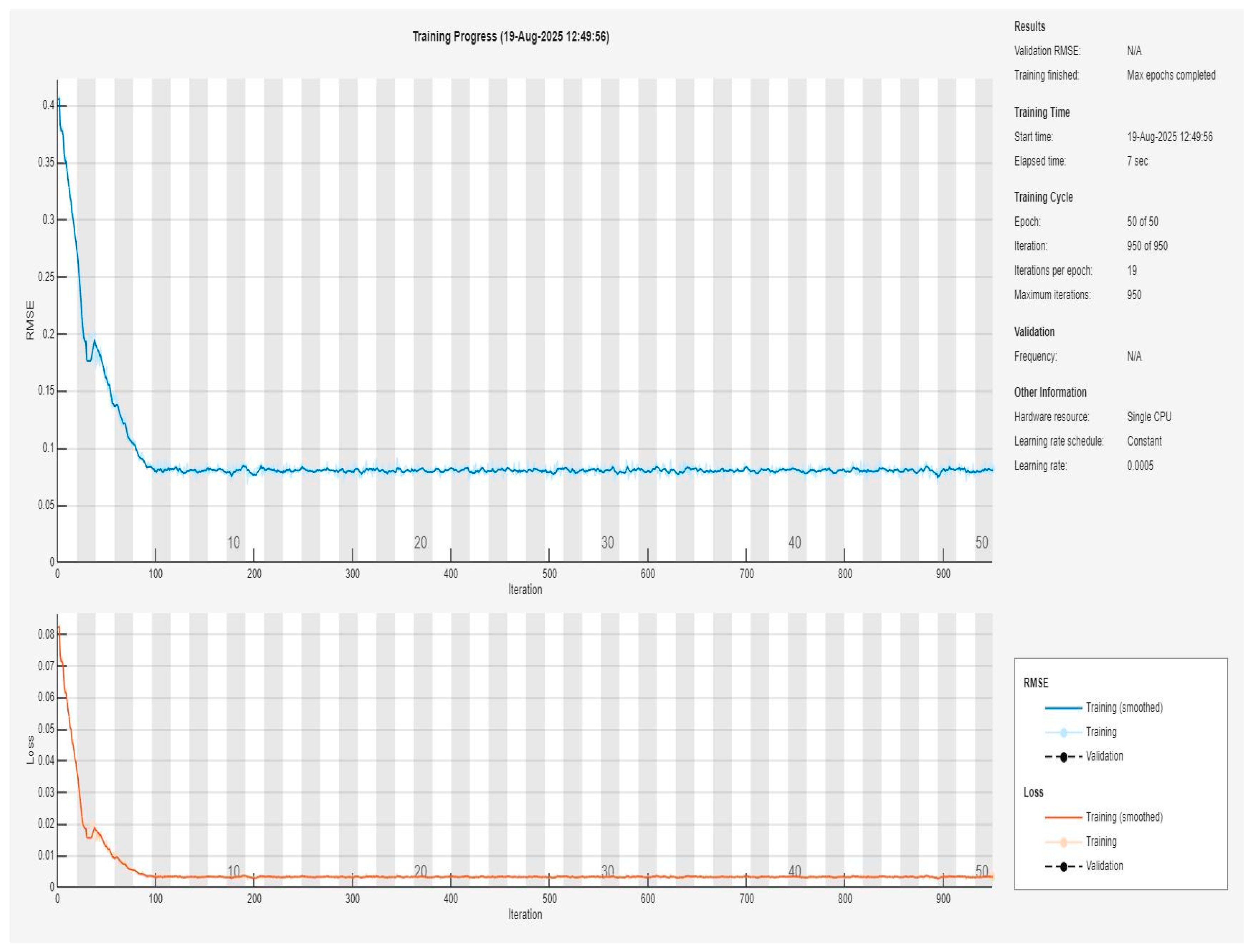
Figure A2.
Decision rules—DLNN-PEA approach (error thresholds set to <4%) with Romanian-based calibration, where risk aversion parameter (σ) is set to 1.5.
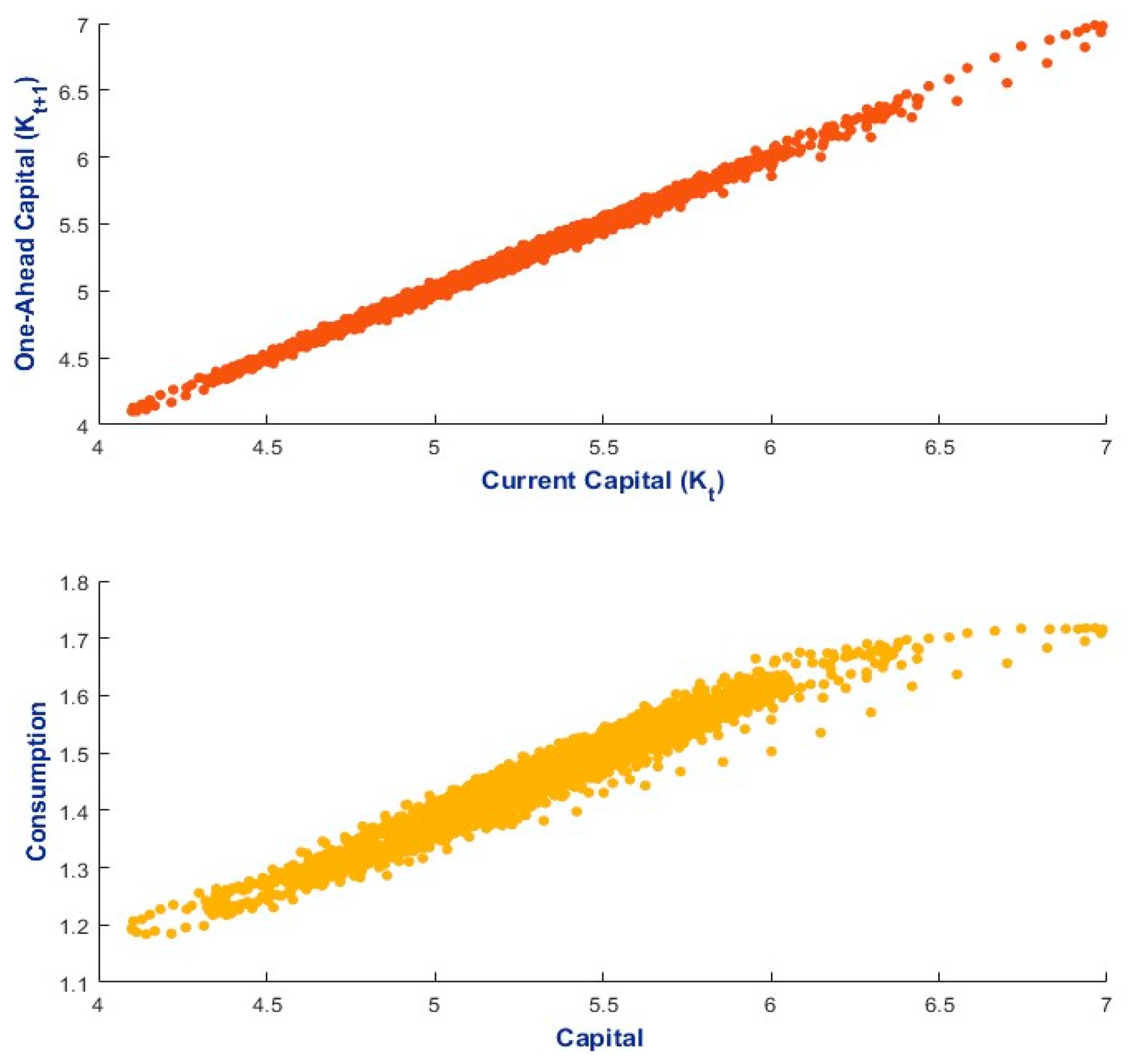
Figure A3.
Empirical probability density functions for capital and consumption—DLNN-PEA approach (error thresholds set to <4%) with Romanian-based calibration, where risk aversion parameter (σ) is set to 1.5.
Appendix B. Supplementary Figures for the DLNN-PEA with = 2
Figure A4.
Initial training of the DLNN-PEA for the Romanian-based calibration with risk aversion parameter (σ) set to 2.
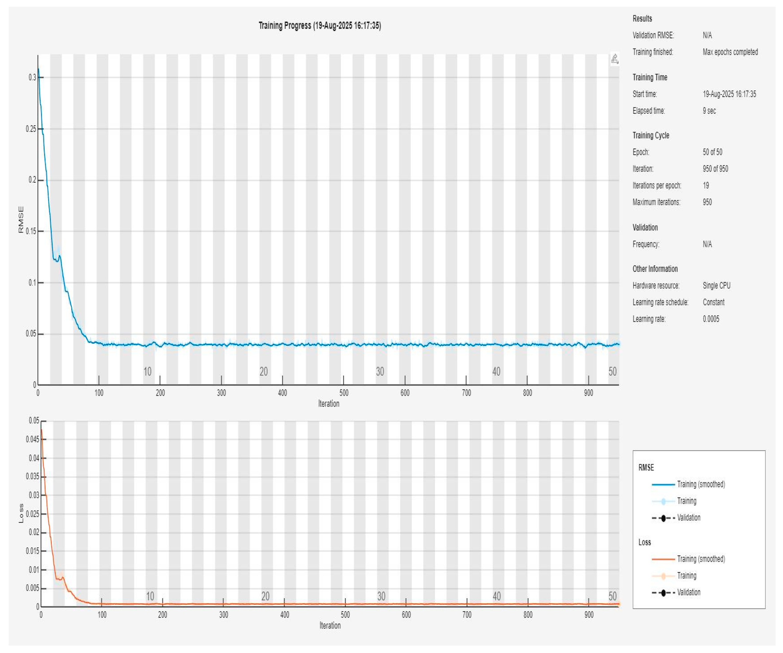
Figure A5.
Decision rules—DLNN-PEA approach (error thresholds set to <4%) with Romanian-based calibration, where risk aversion parameter (σ) is set to 2.
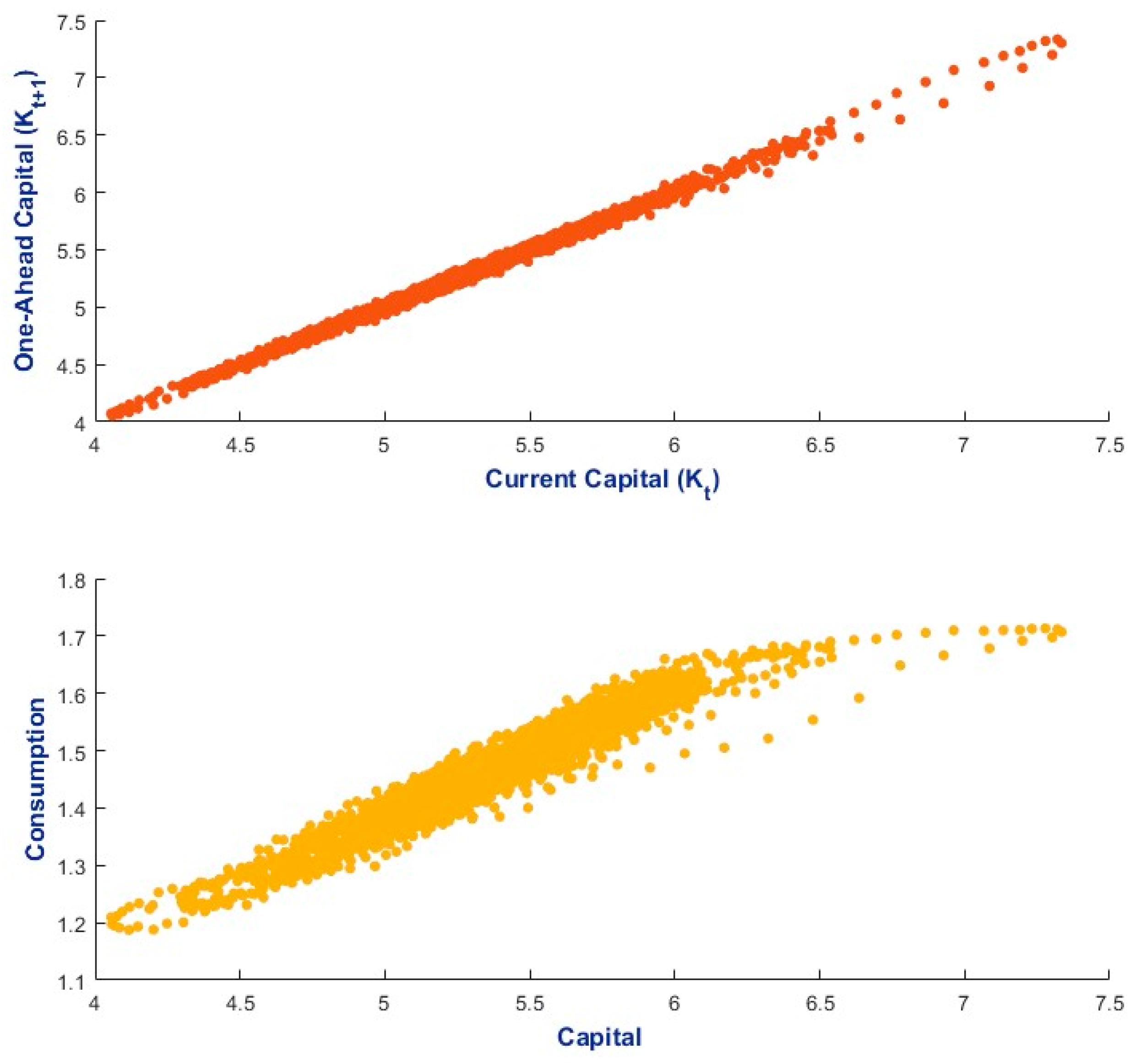
Figure A6.
Empirical probability density functions for capital and consumption—DLNN-PEA approach (error thresholds set to <4%) with Romanian-based calibration, where risk aversion parameter (σ) is set to 2.
Appendix C. Supplementary Figures for the DLNN-PEA with = 2.5
Figure A7.
Initial training of the DLNN-PEA for the Romanian-based calibration with risk aversion parameter (σ) set to 2.5.
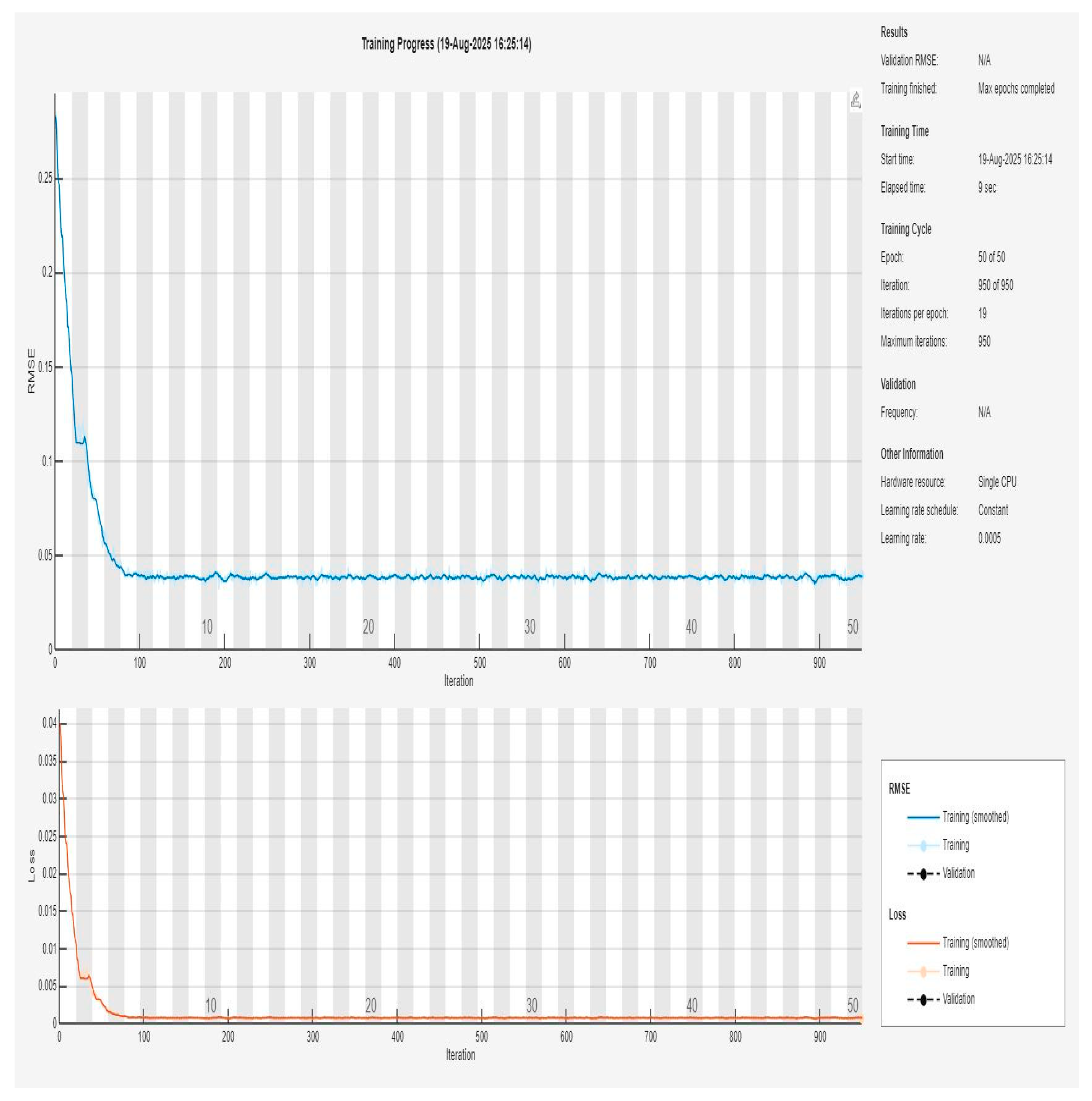
Figure A8.
Decision rules—DLNN-PEA approach (error thresholds set to <4%) with Romanian-based calibration, where risk aversion parameter (σ) is set to 2.5.
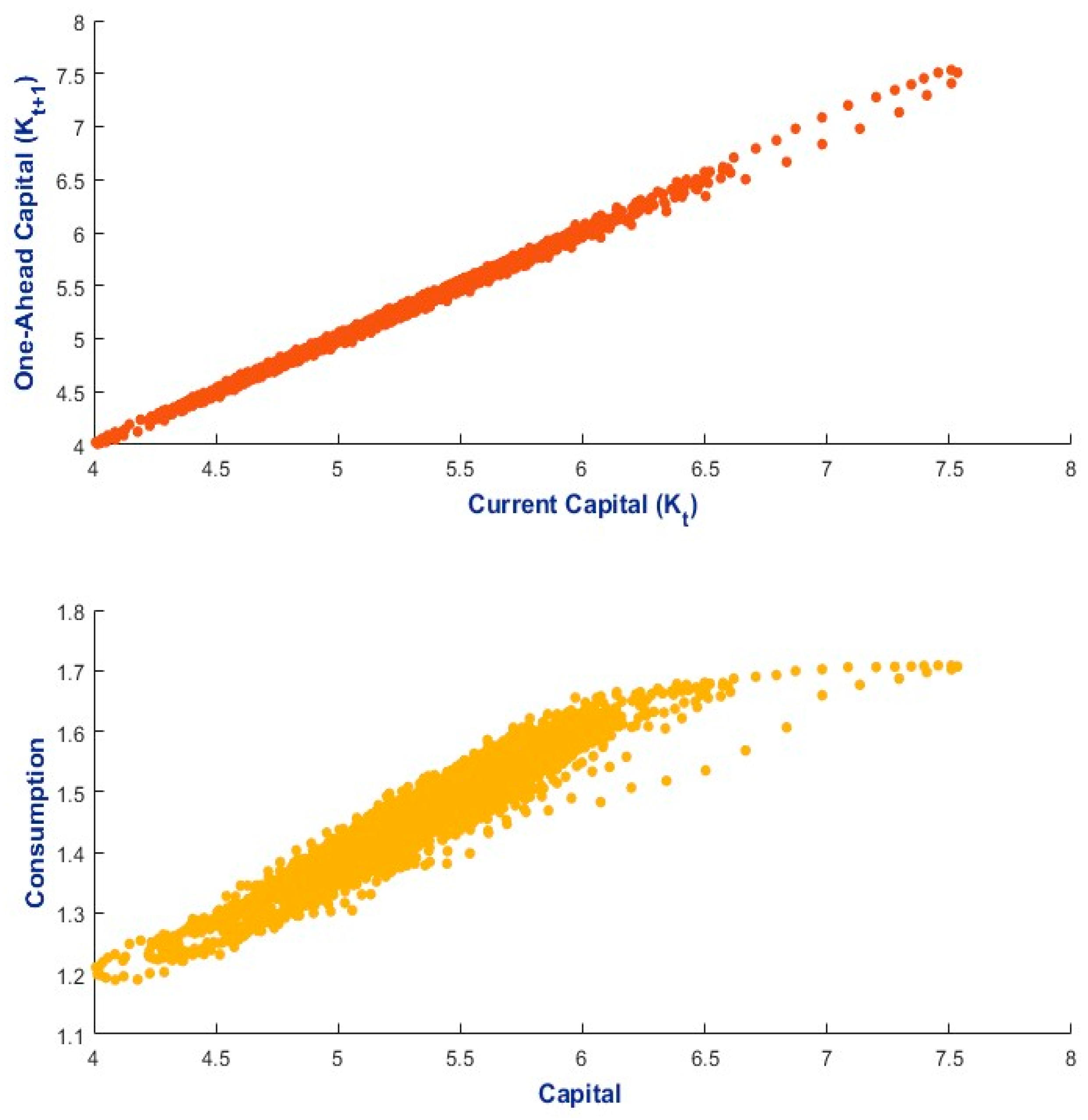
Figure A9.
Empirical probability density functions for capital and consumption—DLNN-PEA approach (error thresholds set to <4%) with Romanian-based calibration, where risk aversion parameter (σ) is set to 2.5.
Appendix D. Supplementary Figures for the DLNN-PEA with = 3
Figure A10.
Initial training of the DLNN-PEA for the Romanian-based calibration with risk aversion parameter (σ) set to 3.
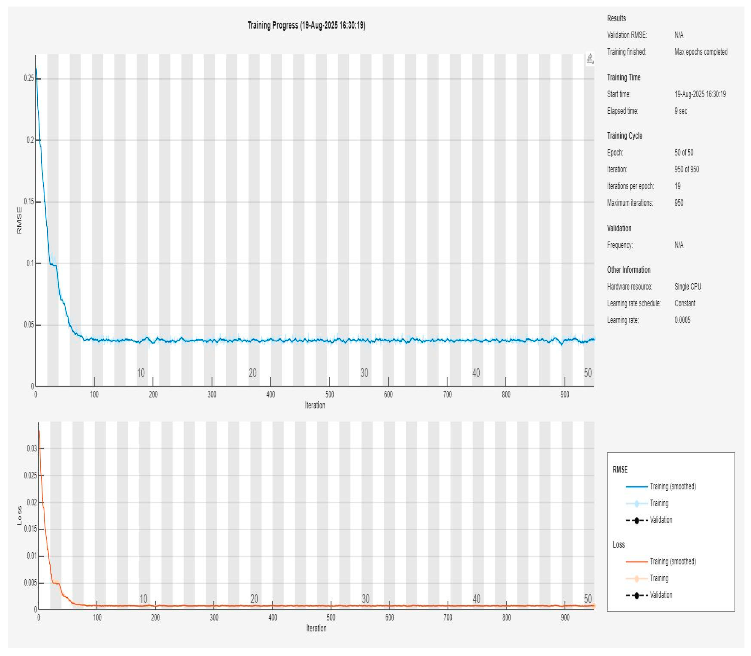
Figure A11.
Decision rules—DLNN-PEA approach (error thresholds set to <4%) with Romanian-based calibration, where risk aversion parameter (σ) is set to 3.
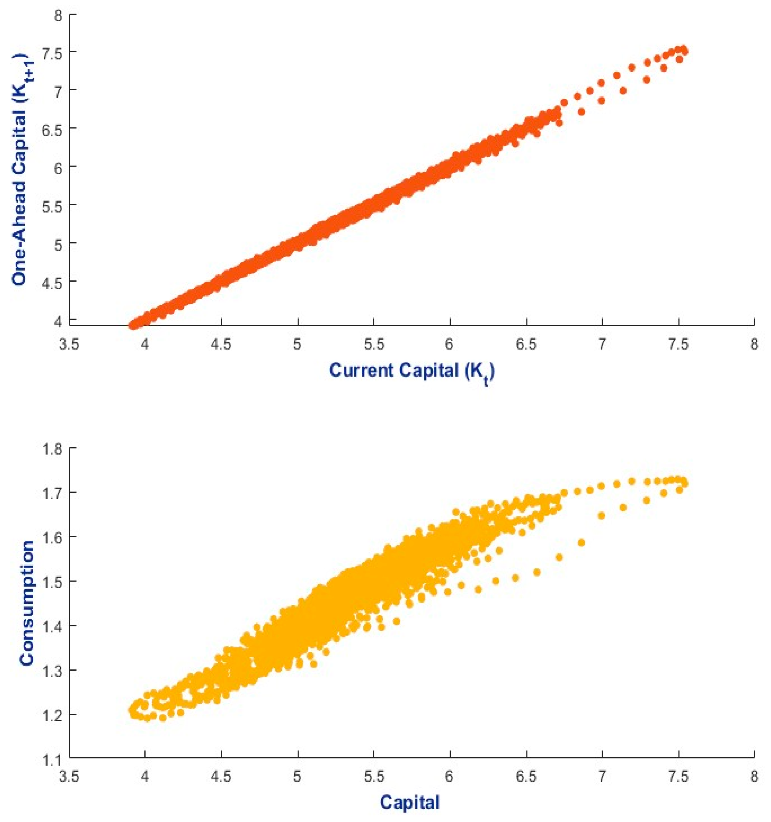
Figure A12.
Empirical probability density functions for capital and consumption—DLNN-PEA approach (error thresholds set to <4%) with Romanian-based calibration, where risk aversion parameter (σ) is set to 3.
References
- Duffy, J.; McNelis, P.D. Approximating and simulating the stochastic growth model: Parameterized expectations, neural networks, and the genetic algorithm. J. Econ. Dyn. Control 2001, 25, 1273–1303. [Google Scholar] [CrossRef] [Scilit]
- Sirakaya, S.; Turnovsky, S.; Alemdar, M.N. Feedback approximation of the stochastic growth model by genetic neural networks. Comput. Econ. 2006, 27, 185–206. [Google Scholar] [CrossRef] [Scilit]
- Vancsura, L.; Tatay, T.; Bareith, T. Navigating AI-Driven Financial Forecasting: A Systematic Review of Current Status and Critical Research Gaps. Forecasting 2025, 7, 36. [Google Scholar] [CrossRef] [Scilit]
- Schmitt-Grohé, S.; Uribe, M. Solving dynamic general equilibrium models using a second-order approximation to the policy function. J. Econ. Dyn. Control 2004, 28, 755–775. [Google Scholar] [CrossRef] [Scilit]
- Dou, W.W.; Fang, X.; Lo, A.W.; Uhlig, H. Macro-finance models with nonlinear dynamics. Annu. Rev. Financ. Econ. 2023, 15, 407–432. [Google Scholar] [CrossRef] [Scilit]
- Duarte, V.; Duarte, D.; Silva, D.H. Machine learning for continuous-time finance. Rev. Financ. Stud. 2024, 37, 3217–3271. [Google Scholar] [CrossRef] [Scilit]
- Maliar, L.; Maliar, S.; Winant, P. Deep learning for solving dynamic economic models. J. Monet. Econ. 2021, 122, 76–101. [Google Scholar] [CrossRef] [Scilit]
- Azinovic, M.; Gaegauf, L.; Scheidegger, S. Deep equilibrium nets. Int. Econ. Rev. 2022, 63, 1471–1525. [Google Scholar] [CrossRef] [Scilit]
- Fernández-Villaverde, J.; Hurtado, S.; Nuño, G. Financial frictions and the wealth distribution. Econometrica 2023, 91, 869–901. [Google Scholar] [CrossRef] [Scilit]
- Ashwin, J.; Beaudry, P.; Ellison, M. Neural network learning for nonlinear economies. J. Monet. Econ. 2024, 144, 103723. [Google Scholar] [CrossRef] [Scilit]
- Sargent, T.J.; Yang, Z. Machine Learning a Ramsey Plan. Q. Rev. 2025, 45, 1–22. Available online: http://www.tomsargent.com/research/calvo_ml_main.pdf (accessed on 28 July 2025). [CrossRef] [Scilit]
- Marcet, A. Solving Non-Linear Stochastic Models by Parameterizing Expectations: An Application to Asset Pricing with Production, Carnegie Mellon University. 1988. Available online: http://hdl.handle.net/10230/20796 (accessed on 28 July 2025).
- den Haan, W.J.; Marcet, A. Solving the stochastic growth model by parameterizing expectations. J. Bus. Econ. Stat. 1990, 8, 31–34. [Google Scholar] [CrossRef] [Scilit]
- Maliar, L.; Maliar, S. Parameterized expectations algorithm and the moving bounds. J. Bus. Econ. Stat. 2003, 21, 88–92. [Google Scholar] [CrossRef] [Scilit]
- Valaitis, V.; Villa, A.T. A machine learning projection method for macro-finance models. Quant. Econ. 2024, 15, 145–173. [Google Scholar] [CrossRef] [Scilit]
- Akash, S.; Sindhu, V.; Pavithra, S. A Projection-Based Framework for Integrating Machine Learning into Macro Finance Models. In Proceedings of the 2025 International Conference on Data Science, Agents & Artificial Intelligence (ICDSAAI), Chennai, India, 28–29 March 2025; IEEE: New York, NY, USA, 2025; pp. 1–4. [Google Scholar] [CrossRef] [Scilit]
- Ali, I.; Khan, S.U. Asymptotic behavior of three connected stochastic delay neoclassical growth systems using spectral technique. Mathematics 2022, 10, 3639. [Google Scholar] [CrossRef] [Scilit]
- Smirnov, R.G.; Wang, K.; Wang, Z. The Cobb-Douglas production function for an exponential model. In Advances in Econometrics, Operational Research, Data Science and Actuarial Studies: Techniques and Theories; Terzioğlu, M.K., Ed.; Springer International Publishing: Cham, Switzerland, 2022; pp. 1–12. [Google Scholar] [CrossRef] [Scilit]
- Medina-López, A.; Jiménez-Partearroyo, M.; Cámara, Á. A Dynamic CGE Model for Optimization in Business Analytics: Simulating the Impact of Investment Shocks. Mathematics 2023, 12, 41. [Google Scholar] [CrossRef] [Scilit]
- Marcet, A.; Lorenzoni, G. Parameterized expectations approach; some practical issues. In Computational Methods for the Study of Dynamic Economies; Marimon, R., Scott, A., Eds.; Oxford University Press: Oxford, UK, 1999; pp. 143–171. [Google Scholar]
- Berardi, M.; Duffy, J. Real-time, adaptive learning via parameterized expectations. Macroecon. Dyn. 2015, 19, 245–269. [Google Scholar] [CrossRef] [Scilit]
- Stone, M.H. The generalized Weierstrass approximation theorem. Math. Mag. 1948, 21, 237–254. [Google Scholar] [CrossRef] [Scilit]
- Ferguson, L.B. Uniform approximation by polynomials with integral coefficients I. Pac. J. Math. 1968, 27, 53–69. [Google Scholar] [CrossRef] [Scilit]
- Averina, T. Conditional optimization of algorithms for estimating distributions of solutions to stochastic differential equations. Mathematics 2024, 12, 586. [Google Scholar] [CrossRef] [Scilit]
- Copaciu, M.; Nalban, V.; Bulete, C. REM 2.0, An estimated DSGE model for Romania. In Proceedings of the 11th Dynare Conference, Brussels, Belgium, 28–29 September 2015; Available online: https://faculty.wcas.northwestern.edu/lchrist/course/Gerzensee_2021/Copaciu_Nalban_Bulette.pdf (accessed on 28 July 2025).

Disclaimer/Publisher’s Note: The statements, opinions and data contained in all publications are solely those of the individual author(s) and contributor(s) and not of MDPI and/or the editor(s). MDPI and/or the editor(s) disclaim responsibility for any injury to people or property resulting from any ideas, methods, instructions or products referred to in the content. |
© 2025 by the authors. Licensee MDPI, Basel, Switzerland. This article is an open access article distributed under the terms and conditions of the Creative Commons Attribution (CC BY) license (https://creativecommons.org/licenses/by/4.0/).