Article

A Domain-Adversarial Mechanism and Invariant Spatiotemporal Feature Extraction Based Distributed PV Forecasting Method for EV Cluster Baseline Load Estimation

1
Electric Power Science Research Institute, State Grid Jibei Electric Power Co., Ltd., Beijing 100045, China
2
Tangshan Power Supply Company, State Grid Jibei Electric Power Co., Ltd., Tangshan 063000, China
3
State Grid Jibei Electric Power Co., Ltd., Beijing 100045, China
4
State Grid Jibei Clean Energy Vehicle Service (Beijing) Co., Ltd., Beijing 100053, China
5
Department of Electrical Engineering, North China Electric Power University, Beijing 071003, China
6
Yanzhao Electric Power Laboratory, North China Electric Power University, Beijing 071003, China
*
Authors to whom correspondence should be addressed.
Electronics 2025, 14(23), 4709; https://doi.org/10.3390/electronics14234709 (registering DOI)
Submission received: 22 November 2025 / Revised: 25 November 2025 / Accepted: 26 November 2025 / Published: 29 November 2025

Abstract

Against the backdrop of high-penetration distributed photovoltaic (DPV) integration into distribution networks, the limited measurability of small-scale DPV systems poses significant challenges to accurately estimating the baseline load of electric vehicle (EV) clusters. To address this issue, effective forecasting of DPV power output becomes essential. This paper proposes a domain-adversarial architecture for ultra-short-term DPV power prediction, designed to support baseline load estimation for EV clusters. The power output of DPV systems is influenced by scattered geographical distribution and abrupt weather changes, leading to complex spatiotemporal distribution shifts. These shifts result in a notable decline in the generalization capability of traditional models that rely on historical statistical patterns. To enhance the robustness of models in complex and dynamic environments, this paper proposes a domain-adversarial architecture for ultra-short-term DPV power forecasting, explicitly designed to address spatiotemporal distribution shifts by extracting spatiotemporal invariant features robust to distribution shifts. First, a Graph Attention Network (GAT) is utilized to capture spatial dependencies among PV stations, characterizing asynchronous power fluctuations caused by factors such as cloud movement. Next, the spatiotemporally fused features generated by the GAT are adaptively partitioned into multiple distribution domains using Hierarchical Density-Based Spatial Clustering of Applications with Noise (HDBSCAN), providing pseudo-supervised signals for subsequent adversarial learning. Finally, a Temporal Convolutional Network (TCN)-based domain-adversarial mechanism is introduced, where gradient reversal training forces the feature extractor to discard domain-specific characteristics, thereby effectively extracting spatiotemporal invariant features across domains. Experimental results on real-world distributed PV datasets validate the effectiveness of the proposed method in improving prediction accuracy and generalization capability under transitional weather conditions.

1. Introduction

1.1. Background and Motivation

With the global energy transition accelerating, distributed photovoltaics (DPVs) have become crucial power generation facilities for establishing a zero-carbon energy system and play a key role in new-type power systems [1]. As of March 2025, China’s installed renewable energy capacity reached 1.966 billion kilowatts, accounting for approximately 57.3% of the country’s total installed capacity. The total installed capacity of DPV in China exceeded 410 million kilowatts, representing 43% of the total photovoltaic (PV) installed capacity [2]. The increasing penetration of DPV in distribution networks means that many electric vehicle (EV) charging stations now host numerous small-scale DPV systems. These DPV systems are often installed behind the meter (BTM), where PV generation and local load are typically not metered separately, forming integrated “DPV + charging load” hybrid units. When multiple such charging stations cluster within a region, their aggregate net load presented to the grid becomes the superposition of DPV output and EV charging load [3]. This superposition renders traditional methods for estimating cluster baseline load ineffective and significantly reduces estimation accuracy [4]. Furthermore, existing load forecasting methods for EV clusters often fail to adequately account for the stochastic fluctuations of DPV, leading to substantial deviations in baseline load estimates. Accurately predicting the power output of these numerous, highly dispersed DPV systems is therefore critical for improving the accuracy of EV cluster baseline load estimation [5]. However, the high spatial dispersion of DPV, combined with minute-level stochastic power fluctuations caused by dynamic shading effects, significantly increases the challenges of grid dispatch and power accommodation. Specifically, micro-meteorological variations under high dispersion lead to asynchronous power fluctuations in adjacent areas, complicating regional power absorption; while highly stochastic disturbances such as cloud movement and nearby shadows trigger sharp power ramps, threatening distribution network voltage stability [6]. Therefore, high-accuracy ultra-short-term power forecasting, which captures spatiotemporal power variation trajectories 15–30 min in advance, provides a critical decision-making window for dispatch systems: it deciphers spatial correlations to coordinate DPV output and forecasts sudden changes to mitigate operational risks [7,8]. This has emerged as a core technology for overcoming the accommodation bottlenecks of distributed energy resources.

1.2. Literature Review

Existing PV power forecasting methods can be categorized into three types: physical models, statistical models, and machine learning approaches [9]. Physical modeling methods calculate power output using PV conversion equations combined with local meteorological parameters. However, differences in tilt and azimuth angles of distributed rooftop PV systems complicate the calibration of component parameters [10], resulting in high model complexity. Statistical models establish regression forecasts based on correlations between historical power and meteorological data. The statistical model proposed in [11] optimizes forecasting under scenarios with scarce historical data through similar-day selection and Markov probability correction, yet it fails to address the issue of historical pattern failure caused by spatiotemporal distribution shifts. Ref. [12] employed gray relational analysis for feature dimensionality reduction combined with optimization algorithms to significantly enhance support vector machine performance and reduce forecasting errors, but it inadequately captures nonlinear interactions between variables under abrupt weather changes. Machine learning methods have become mainstream due to their strong nonlinear mapping capabilities, among which recurrent neural networks (RNNs) and their variants such as long short-term memory (LSTM) networks are widely used for single-site time series modeling. Ref. [13] proposed a four-kernel deep convolutional neural network that extracts multi-scale temporal features through parallel convolutional kernels of four different sizes, achieving high-precision power forecasting, though it did not investigate the impact of local weather in different regions on forecasting bias. Ref. [14] introduced a probabilistic forecasting model based on coupled input-forget-gate networks and quantile regression, enabling probability density forecasting and confidence interval generation for PV power. However, it exhibits large forecasting errors under highly volatile weather conditions.
In recent years, research on DPV power forecasting has primarily focused on temporal modeling, constructing forecasting models by mining historical power output sequences and local meteorological data of PV stations. However, as the penetration of DPV increases, researchers have found that the output of adjacent stations is synergistically influenced by regional environmental factors, demonstrating significant geographical correlation. This spatial coupling effect has prompted a shift in research paradigm from single-site temporal modeling to multi-site spatiotemporal correlation analysis—complementary and lagged correlations formed among neighboring stations due to the spatial continuity of meteorological elements provide critical spatial feature supplements for forecasting models. Consequently, methods such as using graph neural networks (GNNs) to capture topological relationships between stations and constructing spatiotemporal convolutional networks to integrate regional meteorological satellite data have gradually emerged. The method proposed in [15], based on sub-region division and spatiotemporal correlation modeling, combines graph convolutional networks (GCNs) to extract spatial correlation features and LSTM networks to capture dynamic spatiotemporal evolution patterns, achieving high-precision short-term power forecasting for regional DPV. Ref. [16] introduced a hybrid method based on graph neural networks and an improved Bootstrap technique, using GCN to capture spatial correlations and Bi-LSTM to extract temporal dependencies, achieving accurate spatiotemporal correlation modeling for ultra-short-term interval forecasting of wind power. Ref. [17] employed graph neural networks to model complex spatio-temporal dependencies in transportation networks, integrating multi-source data through information fusion techniques to enhance traffic forecasting accuracy and support urban planning applications. Ref. [18] proposed a double-explored spatio-temporal graph neural network (DEST-GNN) that leverages adaptive graph convolution and sparse attention mechanisms to capture dynamic spatial-temporal correlations among multiple photovoltaic stations, improving intra-hour power forecasting precision.
However, the power output of DPV clusters exhibits complex spatiotemporally inconsistent shifts under localized meteorological disturbances. In the temporal dimension, transient shading phenomena cause minute-scale abrupt fluctuations in single-site power output, resulting in asynchronous shifts in output characteristics between consecutive time intervals [19,20,21,22]. In the spatial dimension, micro-meteorological gradient variations, such as fragmented cloud drift, induce power decoupling among neighboring sites. Under identical irradiation conditions, spatial mismatches emerge, including peak-valley misalignment and phase differences in power fluctuations [23,24,25]. These spatiotemporal distribution shifts create significant feature distribution discrepancies between the spatiotemporal correlations embedded in source-site data and the true output distribution of target sites during future forecasting windows. Such discrepancies hinder models trained directly on source data from effectively extracting discriminative spatiotemporal correlation features critical for accurate power forecasting in target sites and time periods. Existing spatiotemporal forecasting models typically rely on the assumption of identical distribution between source and target sites. Nevertheless, in distributed scenarios, the high stochasticity of localized meteorological abruptions invalidates this premise in real-world forecasting environments. The synergistic effects of non-stationary temporal fluctuations and spatially decaying regional correlations drive non-negligible spatiotemporal shifts in power characteristics. This forces models into the dilemma of capturing instantaneous non-steady-state features [26], ultimately leading to performance degradation due to insufficient cross-domain generalization capability.

1.3. Contribution

Accurate DPV power generation forecasting serves as a key premise and core guarantee for improving the accuracy of electric vehicle baseline load estimation. To address the performance degradation in DPV cluster forecasting caused by spatiotemporal distribution shifts under localized transitional weather conditions, this paper proposes a novel ultra-short-term power forecasting method based on spatiotemporal invariant feature learning and domain-adversarial training.
The main contributions of this work are summarized as follows:
(1)
A GAT-HDBSCAN-TCN domain-adversarial fusion framework is proposed. This framework innovatively integrates dynamic spatial dependency modeling, unsupervised distribution domain partitioning, and spatiotemporal invariant feature extraction, offering an effective solution to spatiotemporal distribution shifts in distributed PV forecasting.
(2)
A dynamic spatial dependency feature extraction and unsupervised domain partitioning strategy is designed. To address the dynamic spatiotemporal correlations among PV stations under disturbances, a GAT is employed to adaptively capture spatial dependencies, overcoming the limitations of static graph models like traditional GCN. Subsequently, the HDBSCAN clustering algorithm is introduced for unsupervised domain partitioning, automatically identifying multiple distribution domains and eliminating the subjectivity of manual domain labeling.
(3)
A feature learning mechanism combining TCN and domain-adversarial training is designed to extract domain-invariant spatiotemporal features. The feature extractor GAT-TCN and domain discriminator are optimized through adversarial competition: the feature extractor generates domain-indistinguishable feature representations, suppressing domain-specific information (e.g., weather conditions or station locations), thereby learning spatiotemporal invariant features that characterize PV output patterns. This significantly enhances the model’s generalization capability.

2. DPV Forecasting Method Considering Spatiotemporal Invariant Feature Modeling

To address the spatiotemporal distribution shifts in DPV systems, this paper proposes an ultra-short-term power forecasting method integrating the GAT-HDBSCAN-TCN architecture, with the overall framework illustrated in Figure 1. The framework comprises three core components: spatiotemporal correlation feature extraction, spatial-temporal feature clustering, and TCN-domain adversarial fusion for DPV power forecasting.
(1)
Spatiotemporal correlation feature extraction: GAT is utilized to dynamically capture spatial dependency features among DPV stations. Attention weights are adaptively calculated based on real-time meteorological and power states of each station, effectively characterizing non-uniform spatial dependencies under localized abrupt weather changes.
(2)
Spatiotemporal feature clustering: The HDBSCAN algorithm is applied to adaptively partition the spatiotemporal feature matrix output by the GAT, identifying distinct distribution domains corresponding to weather patterns. This constructs discriminative domain structures to support subsequent adversarial training.
(3)
TCN-domain adversarial fusion for DPV power forecasting: A domain-adversarial training mechanism is established by combining the TCN with a gradient reversal layer (GRL) and a domain discriminator. This mechanism strips domain-specific variant features from multi-domain data, extracts cross-domain robust spatiotemporal invariant features, and ultimately achieves accurate ultra-short-term PV power forecasting.

2.1. Spatial Correlation Feature Extraction Based on GAT

DPV systems are influenced by cloud movement and abrupt changes in local meteorological conditions, leading to non-synchronous and non-uniform spatiotemporal distribution characteristics of solar irradiance intensity among adjacent stations. This meteorologically driven divergence in power output manifests as observable time-delay effects and distinct spatial irradiance gradients between neighboring stations. Such spatiotemporal distribution shifts become particularly pronounced under transitional weather conditions, such as cloudy, rainy, or snowy weather. In this context, static graph structures with fixed connections struggle to effectively capture the complex and dynamically evolving interdependencies among stations under real-time meteorological variations.
To address the challenge of dynamic representation, this paper introduces the GAT. The key advantage of GAT lies in its built-in attention mechanism, which eliminates the need for explicit reconstruction of graph topology [27,28]. Instead, it allows the network to adaptively learn and dynamically assign association weights between stations during training, based on state features such as irradiance, power output, and meteorological information at each time step. This mechanism enables the model not only to accurately capture instantaneous changes in inter-station influences caused by meteorological events such as cloud movement but also to focus in real time on the information from neighboring stations most relevant under current weather conditions. Through this attention-weighted dynamic interaction modeling, GAT significantly enhances the representation of complex spatiotemporal features in DPV systems, thereby improving the robustness of power forecasting under meteorological fluctuations [29].
To model the dynamic spatial correlations among DPV stations, this paper employs GAT. In the PV application context, each node corresponds to a PV station, with node features including time-series data such as irradiance and power output. GAT dynamically learns the association weights between stations through an attention mechanism, as outlined below:
At the current time step t , for a target PV station i and any neighboring station j , an unnormalized attention coefficient e i j ( t ) is first computed to preliminarily quantify the influence of station j on station i under specific meteorological and power output conditions:
e i j ( t ) = LeakyReLU a T W h i ( t ) | | W h j ( t )
where h i ( t ) and h j ( t ) represent the input feature vectors of stations i and j at time t , respectively; W is a learnable weight matrix applied for adaptive transformation and dimensionality reduction of the raw features; | | denotes vector concatenation; a is a learnable parameter vector defining the attention mechanism; and LeakyReLU introduces nonlinearity to enhance expressive capacity. The coefficient e i j ( t ) essentially reflects the instantaneous correlation strength between the output patterns of the two stations under dynamic meteorological conditions [30].
To ensure comparability of attention weights across different neighbor nodes and adherence to a probability distribution, the attention coefficients for all neighbors j of target station   i are normalized using the softmax function over all neighbors in the set N i , where N i represents the set of all neighboring nodes of station i :
α i j ( t ) = e x p ( e i j ( t ) ) k N i e i k ( t )
The normalized attention weight α i j ( t )   represents the dynamic influence intensity of station j on station i at time t .
This mechanism offers critical advantages in PV scenarios: when moving cloud masses cause a simultaneous power drop in region A while adjacent region B maintains high output, the model can automatically increase the weights within region A while reducing the weights between regions A and B—even if they are geographically adjacent. Conversely, the weights of geographically dispersed regions A that are influenced by the same weather system can be significantly enhanced. This approach transcends the limitations of fixed geographical distances or correlation coefficient thresholds, enabling precise capture of the nonlinear and instantaneous spatial correlations among PV stations under weather disturbances. Thereby, it effectively models and compensates for spatial distribution shifts in power output.
Using the learned dynamic weights α i j ( t ) , the updated feature representation h i ( t ) of the target station i at time t is obtained by aggregating the transformed features of all its neighbor stations and applying a nonlinear activation function   σ :
h i ( t ) = σ j N i α i j ( t ) W h j ( t )
This aggregation process ensures that the new features of station ii not only encapsulate its own state but also integrate the weighted influences from all other stations at the current time step, thereby deeply encoding dynamic spatial correlation information [31].
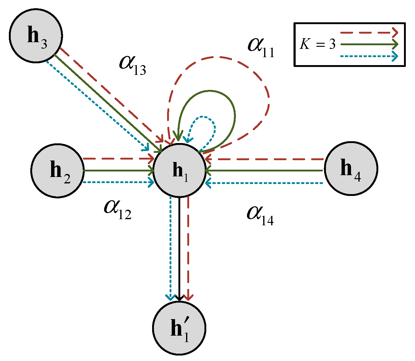
To further enhance the model’s robustness and representational capacity, GAT introduces a multi-head attention mechanism: multiple sets of the above attention computation are executed independently and in parallel, and the output features of the   K heads are either concatenated or averaged to form the final feature representation of the station:
h i ( t ) = σ 1 K k = 1 K j N i α i j ( t ) W k h j ( t )
The multi-head mechanism allows the model to learn diverse inter-station correlation patterns in different feature subspaces in parallel, thereby more comprehensively capturing complex meteorology–power coupling characteristics and enhancing the modeling capability under transitional weather conditions. The multi-head attention mechanism is schematically shown in Figure 2:
After processing through the GAT layer, the output node feature matrix H ( t ) is obtained:
H ( t ) = h 1 ( t ) , h 2 ( t ) , , h N ( t ) T
H ( t ) represents the dynamic spatial correlations among PV stations learned via the attention mechanism at time t . Given the strong temporal dependence of PV power, stacking the output feature matrices of GAT over consecutive T time steps along the temporal dimension forms a three-dimensional feature tensor, which serves as the input for subsequent temporal modeling modules.

2.2. Spatiotemporal Feature Clustering Based on HDBSCAN

Influenced by transitional weather conditions, DPV power exhibits significant spatiotemporal distribution shifts, resulting in non-stationary data distributions. Uniformly modeling the entire power sequence makes it difficult to effectively capture salient features amid dynamic changes, thereby constraining forecasting accuracy and generalization capability. This paper proposes a domain division framework based on spatiotemporal feature clustering: by performing cluster analysis on the three-dimensional spatiotemporal feature sequences of PV power, segments with similar statistical distributions are grouped into the same domain. This strategy aims to construct data subsets with homogeneous distributions while laying the foundation for domain-adversarial training.
Traditional K-Means clustering is difficult to adapt to the requirements of this scenario due to its inherent limitations: on the one hand, it requires predefining the number of clusters, while the complex distribution of spatiotemporal features makes it difficult to predetermined the optimal number of divisions [32]; on the other hand, it is sensitive to variations in cluster shape and density, and cannot effectively handle non-spherical clusters and uneven density distributions that may exist in the three-dimensional feature space [33]. In view of this, this paper employs HDBSCAN. This algorithm, based on the concept of density-based clustering, overcomes parameter sensitivity issues through an automated hierarchical clustering process. Its core advantages include: no need to preset the number of clusters, ability to identify clusters of arbitrary shapes, adaptive handling of multi-density distributions, and robust resistance to noise interference [34,35].
HDBSCAN constructs the cluster structure through density connectivity, with its core process regulated jointly by the neighborhood radius ε and the minimum density threshold m. Given a dataset D containing N samples:
D = x 1 , , x N
The Euclidean distance between any two points is first calculated:
d x i , x j = k = 1 3 x i k x j k 2
Based on this, the ε-neighborhood of a sample x i is defined as:
N ε x i = x i D | d x i , x j ε
When the neighborhood density satisfies N ε x i     m , x i is identified as a core point. The algorithm then constructs a density-reachable graph: if there exists a sequence of core points p 1 ,   p 2 , , p k such that p k + 1 N ε p t     ( 1 t < k ) , then p 1 and p k are said to be density-reachable. All density-reachable core points and the boundary points within their ε-neighborhoods are merged into the same cluster. Points that do not meet the core point condition and are not covered by the neighborhood of any core point are considered noise points.
The final generated cluster structures C 1 , , C K form a hierarchical topology partitioned by density boundaries in the feature space, mathematically represented as:
D = k = 1 K C K N n o i s e ,   i     j ,   C i C j =
The spatiotemporal domain partitioning generated by HDBSCAN automatically produces pseudo-domain labels with clear physical significance through the construction of a hierarchical density-based cluster structure. These labels serve as supervisory signals, replacing traditional manual division methods, enabling the domain discriminator to be trained based on data-driven real distribution differences [36]. More importantly, the clustering process constructs clear decision boundaries in the feature space by maximizing intra-domain homogeneity and inter-domain heterogeneity. This structured partitioning can effectively suppress the interference of domain-related features on the predictive model, decoupling essential features possessing spatiotemporal invariance, and provides crucial support for subsequent domain-adversarial training [37].

2.3. DPV Power Forecasting Based on Temporal Convolutional Network and Domain Adversarial Fusion

The output power of DPV power stations is significantly influenced by geographical location and meteorological conditions, leading to complex spatiotemporal multi-dimensional shifts in their data distribution. Such distribution shifts substantially degrade the generalization performance of forecasting models on unseen stations or during new time periods. To address this challenge, this study introduces a domain-adversarial training mechanism, whose core objective is to guide the model to learn essential features that are insensitive to spatiotemporal variations, i.e., spatiotemporal invariant features, thereby enhancing the model’s robustness against distribution discrepancies.
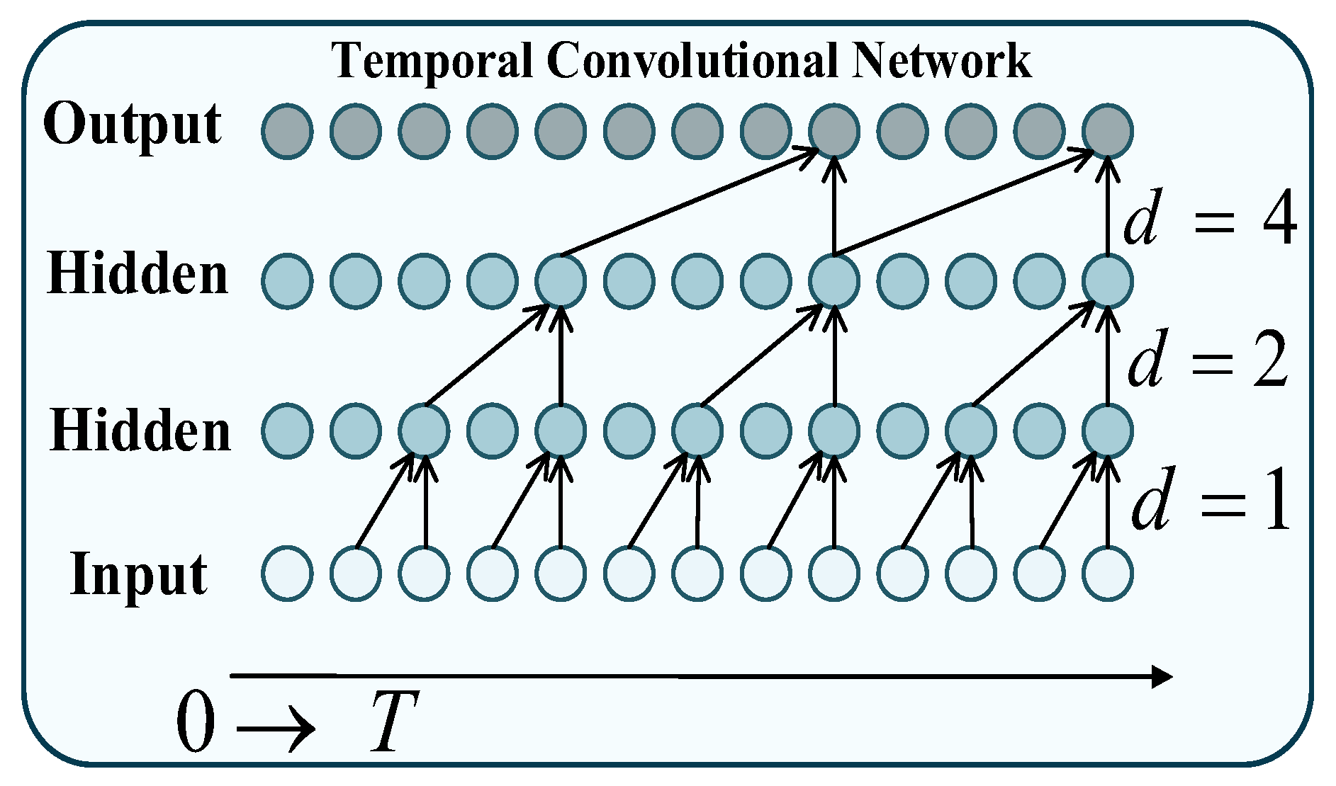
This domain-adversarial architecture consists of three core components: a feature extractor, a power predictor, and a domain discriminator. The feature extractor is designed to achieve two goals: first, to extract highly discriminative features beneficial for power forecasting; second, to generate feature representations that confuse the judgments of the domain discriminator. In the proposed method, the feature extractor is constructed jointly by GAT and TCN. The GAT layer is responsible for modeling the spatial correlations among PV stations, utilizing an attention mechanism to dynamically compute the influence weights of different neighboring stations on the central station, thereby achieving adaptive spatial feature aggregation and outputting a spatial feature matrix. Spatial features across multiple time steps are stacked to form a spatiotemporal feature tensor. Subsequently, the TCN layer processes this spatiotemporal tensor to capture long-term temporal dependencies [38,39,40,41,42]. The causal convolution structure of TCN is depicted in Figure 3:
The core operation of TCN is dilated causal convolution:
T C N X t = k = 0 K 1 W k · X t d · k
where   X denotes the input sequence, W k represents the convolutional kernel weights, d is the dilation factor, and   K is the kernel size. This structure ensures that the output at time t depends only on inputs at time t and earlier, complying with the requirements of forecasting tasks and effectively capturing long-range temporal patterns. After joint processing by GAT and TCN, the feature extractor outputs a high-dimensional feature representation that integrates critical spatiotemporal information.
The power predictor receives the high-dimensional features from the feature extractor. Its structure typically comprises multiple fully connected layers and nonlinear activation functions (e.g., ReLU), aiming to map the input features to forecasted PV power values for a specific future period.
The domain discriminator performs a multi-class classification task. It receives the same input features as the power predictor and outputs a probability distribution over predefined domains for each sample. Its optimization goal is to accurately identify the true source domain of the samples.
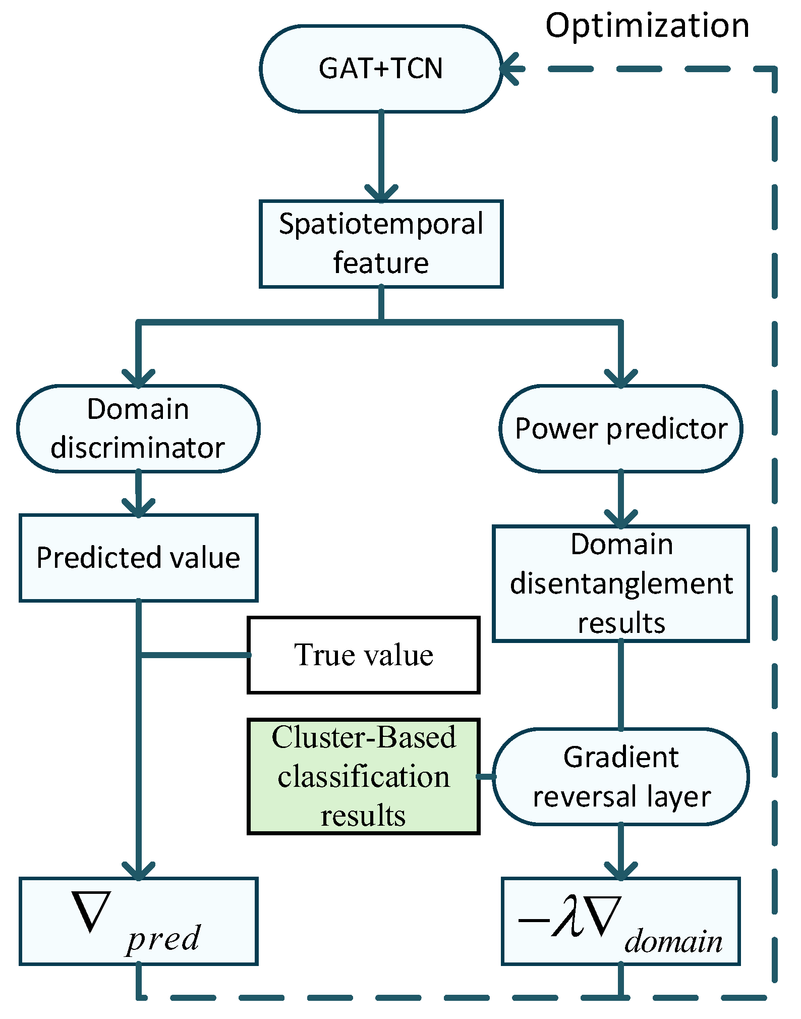
The core mechanism of domain-adversarial training lies in the adversarial optimization process established between the feature extractor and the domain discriminator via a GRL. During forward propagation, the GRL performs an identity operation:
GRL x = I
During backpropagation, the GRL reverses the gradient passed back from the domain discriminator to the feature extractor and multiplies it by a scaling factor λ :
GRL x = λ I
where I is the identity matrix. This implies that when the domain discriminator minimizes its domain classification loss (e.g., cross-entropy loss) through backpropagation, the GRL multiplies the gradient passed back to the feature extractor by λ , causing the parameters of the feature extractor to update in the opposite direction to the optimization objective of the domain discriminator. Consequently, the domain discriminator strives to distinguish the domain sources of the samples, while the feature extractor updates itself based on the reversed gradient signals to generate features that make it difficult for the domain discriminator to accurately identify the source domain of the samples.
The overall training objective of the model is to minimize a composite loss function L t o t a l . Differing from traditional domain adaptation methods that utilize only source domain labels, this study partitions the training data via clustering into multiple domains with known labels. Therefore, the total loss function is defined as the sum of the power forecasting loss and the domain discrimination loss across all domains:
L t o t a l = d = 1 N d L p r e d P d , P ^ d + L d o m a i n D d , D ^ d
where P d and P ^ d represent the actual and forecasted power values for domain d , respectively, and L p r e d is the power forecasting loss function; D d and D ^ d represent the actual domain label and the forecasted domain label probability distribution for domain dd, respectively, and L d o m a i n is the domain discrimination loss function; N d denotes the total number of domains identified by the HDBSCAN clustering algorithm.
During the adversarial optimization process, the feature extractor (GAT+TCN) is driven to learn a balance: on one hand, it must retain the core information crucial for power forecasting to meet the power predictor’s requirement of minimizing L p r e d ; on the other hand, to counteract the domain discriminator, it must suppress or eliminate variant features highly correlated with specific geographical locations or temporal domains. This optimization process ultimately prompts the feature extractor to focus on intrinsic patterns that remain relatively stable across different domains—i.e., the spatiotemporally invariant features. These features capture the fundamental physical principles of PV power generation, rather than the superficial noise of specific spatiotemporal scenarios. The domain-adversarial mechanism is presented in Figure 4:
In summary, by integrating the spatial attention mechanism of GAT, the long-term temporal modeling capability of TCN, and the optimization objective of the domain-adversarial mechanism, the proposed method can effectively extract robust spatiotemporally invariant features from DPV power data. These features significantly enhance the generalization performance and forecasting accuracy of the forecasting model under unseen data distributions, such as new power stations or future time periods, providing an effective solution to the problem of spatiotemporal distribution shift.

3. Case Study

3.1. Data Description and Implementation Details

The experimental data were obtained from DPV base in Inner Mongolia, China, comprising the time-series power generation data of DPV power stations from July 2024 to June 2025, with a temporal resolution of 15 min. The rated capacity of each station is 6 MW. A small number of missing data points were processed using linear interpolation. Finally, the normalized data were divided into training, validation, and test sets with a ratio of 8:1:1. The power data were standardized by dividing by the rated capacity of a single station, resulting in the “Standardized Power” shown in Figure 5 and Figure 6.

3.2. Evaluation Metrics

Based on the actual power data and the corresponding forecasted power data, the Normalized Root Mean Square Error (NRMSE) and the Normalized Mean Absolute Error (NMAE) were calculated to quantify the accuracy of the forecasting results [43]. The specific formulas are as follows:
N R M S E = 1 P m a x 1 N t = 1 N P actual , t P predicted , t 2
N M A E = 1 N P max t = 1 N P actual , t P predicted , t
where N represents the total number of samples, t is the time index, P actual , t denotes the actual power value at time t , P predicted , t denotes the model forecasted power value at time t , and P max represents the maximum value of the actual power data.

3.3. Benchmarks Configuration

To demonstrate the effectiveness of the proposed method, several forecasting methods were utilized for ultra-short-term PV power forecasting. The forecasting results from one specific power station are taken as an example. The configurations of each comparative method are as follows:
Method 1 (M1): The power output of each PV station is used as node features. A GCN is employed for modeling and forecasting to obtain the power output of the target station.
Method 2 (M2): The power output of each PV station is used as node features, considering the spatial distribution shift among the outputs of different PV stations. A GAT is employed for modeling and forecasting to obtain the power output of the target station.
Method 3 (M3): The power output of each PV station is used to determine the input node features. A GAT model is used for forecasting, considering both the temporal distribution shift and spatial distribution shift in the PV power sequences. A domain-adversarial mechanism is adopted to extract temporally invariant features, obtaining the power output of the target station.
Method 4 (M4): The proposed PV power forecasting method considering spatiotemporal distribution shifts. The power output of each PV station is used to establish the node features, and a domain-adversarial mechanism is employed to extract spatiotemporally invariant features, obtaining the power output of the target station.
The detailed configurations of all comparative methods are summarized in Table 1:

3.4. The Results and Analysis of Regional Forecasting

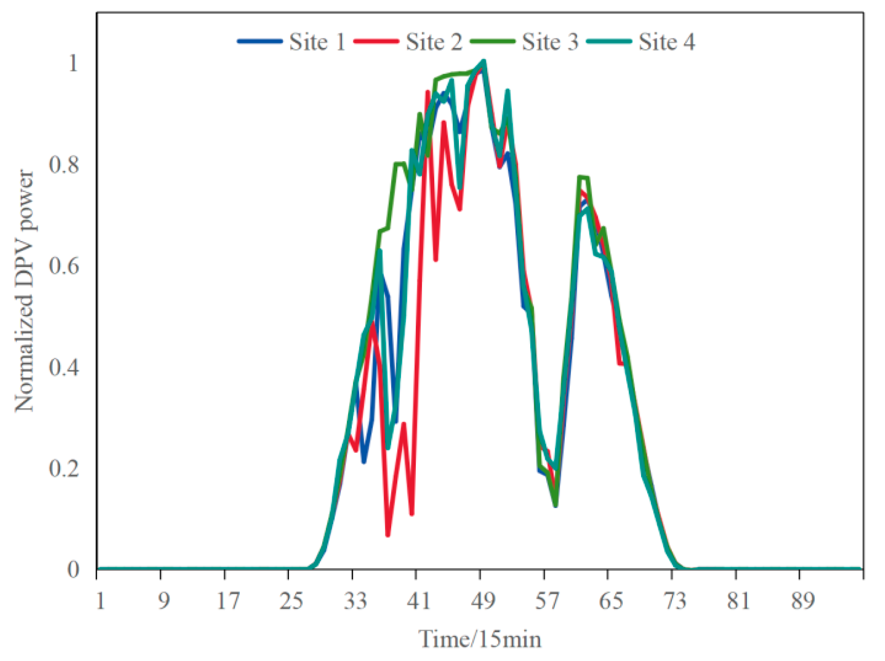
The standardized power fluctuation curves of four adjacent PV power stations on the same day are shown in the figure. It can be observed that the fluctuation patterns of the four stations exhibit largely consistent behavior from afternoon to evening. However, varying degrees of fluctuation occur from morning to noon: Station 2 exhibits the most violent fluctuations, whereas Station 3 shows the smallest amplitude. The fluctuations of Stations 1 and 4 are the most consistent. Therefore, it can be concluded that although the fluctuation patterns of each station exhibit spatial correlation and share a high degree of overall trend similarity, there are noticeable lead or lag differences in the specific timing of their fluctuations, i.e., spatial asynchrony. This phenomenon primarily stems from the direct influence of solar radiation on PV power output: the formation and movement of clouds dynamically alter the irradiance reaching the Earth’s surface, thereby causing temporal misalignment in the power output of stations at different geographical locations.
Figure 5 displays the standardized power fluctuation curves of the same DPV power station under different weather conditions. It can be seen that the power distribution of the same PV station differs significantly under different meteorological conditions. Specifically, during noon on sunny days, the actual power approaches the peak value, and the overall curve is relatively smooth. Under rainy/snowy weather conditions, the actual power remains consistently low with high fluctuation frequency but small amplitude, the maximum fluctuation not exceeding 0.2. In contrast, under cloudy conditions, the power fluctuates violently during the corresponding period with a larger amplitude, the maximum fluctuation exceeding 0.6. These phenomena indicate that random weather changes can significantly alter the output characteristics at specific time points, leading to temporal distribution shifts, which increases the difficulty for traditional forecasting models to accurately capture their dynamic patterns.
Such spatiotemporal distribution shifts weaken the correlation between historical data and future data states, limiting the generalization capability of forecasting models trained on historical data when dealing with future variations. Therefore, to enhance the stability and accuracy of PV power forecasting, it is necessary to introduce optimization strategies in the modeling process that can adapt to the spatiotemporal shift characteristics under different weather conditions. Subsequent sections of this paper will conduct an in-depth study on the PV power forecasting problem involving spatiotemporal distribution shifts.
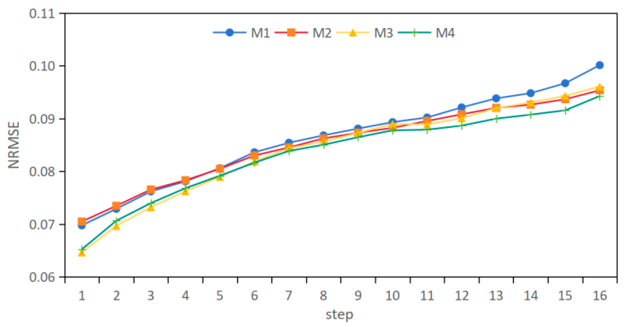
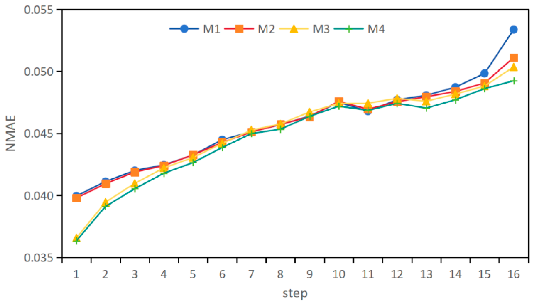
Table 2 and Table 3 present the NRMSE and NMAE metrics of different methods across multiple forecasting horizons. An analysis of these results shows that at the shortest forecasting horizon of 15 min, Method 3 performs best in terms of the NRMSE metric. However, as the forecasting horizon extends to 4 h, the comprehensive advantage of Method 4 becomes apparent. Its NRMSE and NMAE values are consistently the lowest across all forecasting horizons, significantly outperforming the other methods.
The magnitude of the forecasting errors reflects the differing capabilities of each method in handling spatiotemporal complexity. Method 1 only utilizes graph structures to model the spatial relationships among stations without explicitly addressing spatial or temporal distribution shifts, resulting in a significant increase in error as the forecasting horizon extends, reaching the highest NRMSE of 0.1001 at the 4 h mark. Method 2 partially captures spatial dynamics through an attention mechanism, showing improvement over Method 1 at longer horizons. However, its neglect of temporal distribution shifts limits its forecasting accuracy improvement over extended periods. Method 3 focuses on temporal modeling and shift correction for the target station. Although it excels in short-term forecasting, the lack of TCN’s ability to capture long-term dependencies causes it to be gradually surpassed by Method 4 for forecasts beyond 2 h, highlighting its limitations at longer scales.
The superior performance of Method 4, particularly over longer forecasting horizons, stems from its synergistic approach to addressing spatiotemporal distribution shifts. It not only uses the power output of each PV station to determine the node features and employs GAT to dynamically capture spatial correlations and their shifts among stations but also introduces a TCN to effectively model long-term temporal dependencies. Furthermore, it adopts a domain-adversarial mechanism to jointly extract spatiotemporally invariant features. This end-to-end spatiotemporally invariant feature learning framework effectively suppresses the coupling effects and error accumulation of spatial and temporal shifts during forecasting, thereby demonstrating significant stability and accuracy advantages over extended observation scales. Ultimately, at the 4 h forecasting horizon, the NRMSE of Method 4 is significantly reduced by 5.8% compared to the baseline Method 1, and its NMAE is reduced by 2.4% compared to the next best method. These results strongly validate the effectiveness and advancement of the proposed method in tackling the complex issue of spatiotemporal distribution shifts in PV power forecasting.
Figure 7 and Figure 8 display the variation curves of NRMSE and NMAE for each method across different forecasting horizons (step lengths). At short horizons, the NRMSE and NMAE curves of Method 3 are the lowest within the 15 min to 1 h interval, validating the effectiveness of the domain-adversarial mechanism for power forecasting. However, as the forecasting horizon extends beyond 2 h, the error growth rate of Method 4 slows down significantly. The two curves gradually exhibit a convergent trend, with Method 4 ultimately taking the lead in the 3 to 4 h horizon range. Notably, at the 4 h mark, the NRMSE value of Method 4 drops to 0.0943 and the NMAE value to 0.0492. The performance gap between Method 4 and the second-best method increases as the horizon extends.
This dynamic variation profoundly reflects the differences in model architectures among the methods. Method 1, which does not incorporate any distribution shift correction mechanism, exhibits higher errors. The gap between it and the other methods becomes particularly evident after 2 h, exposing the limitations of traditional graph models in long-term forecasting. Although Method 2 optimizes the modeling of spatial correlations between stations through an attention mechanism, its error remains higher than that of Method 3. This indicates that merely adjusting for spatial feature shifts is insufficient to effectively suppress long-term error accumulation. Although Method 3 utilizes multi-station inputs and incorporates a temporal adversarial mechanism, the upward slope of its curve after the 2 h mark is significantly steeper than that of Method 4. This reflects the difficulty an isolated temporal correction strategy faces in coping with spatiotemporal shift effects over extended time scales.
The superiority of Method 4 stems from its spatiotemporal collaborative mechanism: the GAT dynamically captures spatial distribution shifts, the TCN models long-term temporal dependencies, and the spatiotemporal joint adversarial mechanism decouples the coupling effects of shifts through end-to-end optimization. This design results in the optimal error curve for Method 4, particularly in the long-horizon range, providing visual validation of the optimization effect that spatiotemporally invariant feature extraction has on long-term forecasting stability. While recent dynamic spatio-temporal models excel at capturing instantaneous correlations, the proposed GAT-HDBSCAN-TCN framework demonstrates superior performance in long-term forecasts, particularly under complex weather conditions. This underscores the critical advantage of our method in learning spatiotemporally invariant features that are robust to distribution shifts, beyond merely modeling dynamic dependencies.
To further demonstrate the superiority of the proposed method, Table 4 presents the forecasting errors of all methods under three typical weather conditions: sunny, cloudy, and rainy, revealing the significant impact of meteorological conditions on model performance and the differences in method design. Overall, Method 4 performs excellently across various weather scenarios.
In sunny conditions characterized by stable irradiance and minimal fluctuations, Method 3 achieves the best NRMSE metric at short horizons, confirming the effectiveness of temporal shift correction on stable data. However, when the forecasting horizon extends beyond 3 h, Method 4 surpasses Method 3 by leveraging its capability to capture long-term dependencies, reducing NRMSE by 8.5% compared to Method 3. This indicates that even under stable weather conditions, long-term forecasting still requires support from modeling temporal dependencies. In cloudy scenarios, cloud movement intensifies spatial heterogeneity. In 1h-4h forecasts, Method 4 maintains the lowest or second-lowest NRMSE and NMAE, benefiting from the GAT’s ability to capture dynamic spatial shifts—when cloud shadows cause abrupt output changes at stations, the attention mechanism adaptively adjusts spatial weights, and the spatiotemporal adversarial mechanism further suppresses the error propagation caused by such disturbances. The high volatility of rainy conditions amplifies the differences between methods. The 4h NRMSE of Method 4 is 0.0955, lower than Method 3’s value of 0.1064. This is primarily because the TCN module effectively captures temporal features through dilated convolutions, while the joint spatiotemporal adversarial mechanism effectively decouples the spatiotemporal shift coupling effects induced by the movement of rain clouds.
The increase in meteorological complexity essentially represents an intensification of coupled spatiotemporal distribution shifts and exacerbated spatiotemporal shift phenomena, which directly amplifies the inherent limitations of traditional methods. The core breakthrough of Method 4 lies in establishing a joint suppression mechanism for spatiotemporal shifts by extracting meteorology-invariant spatiotemporal features through the GAT-TCN architecture, enabling domain-adversarial learning to fundamentally decouple the coupled shifts caused by cloud and rain movement. This endows the model with generalized resistance to meteorological disturbances, ultimately leading to its superior performance in the 4h forecast under rainy conditions, validating the critical role of spatiotemporal cooperative modeling in renewable energy power forecasting.

4. Conclusions

The accurate estimation of baseline load for electric vehicle clusters has become increasingly challenging under high-penetration DPV scenarios due to the stochastic and coupled nature of DPV generation and charging loads. To address the performance degradation in forecasting caused by spatiotemporal distribution shifts in DPV clusters under local abrupt weather changes, this paper proposes an ultra-short-term power forecasting method for clustered DPV systems based on spatiotemporally invariant feature-driven learning and GAT-TCN domain-adversarial modeling. This method dynamically captures meteorology-driven nonlinear spatial correlations among stations using GAT, effectively characterizing asynchronous power fluctuations induced by factors such as cloud movement. It then employs HDBSCAN clustering to adaptively partition spatiotemporal features, accurately identifying multimodal distribution domains such as clear-sky, rainy, and snowy conditions. Finally, TCN combined with a gradient reversal-based domain-adversarial mechanism is applied to extract common spatiotemporally invariant features across different distribution domains.
These invariant features characterize the fundamental patterns of PV power generation, significantly enhancing the model’s generalization capability in response to local abrupt weather changes and station heterogeneity. The experimental results demonstrate that the proposed method effectively mitigates the negative impact of spatiotemporal distribution shifts on forecasting accuracy under transitional weather scenarios, providing technical support for stable dispatch and efficient accommodation of high-penetration DPV integration. Future work will focus on optimizing multi-scale feature extraction mechanisms to further improve the model’s robustness under complex meteorological conditions.

Author Contributions

Conceptualization, Z.Z., G.W. and H.R.; Methodology, Z.Z., Q.L., B.B. and P.Y.; Validation, X.L., Z.W., G.W. and H.R.; Formal analysis, Z.W.; Writing—original draft, Q.L., B.B., P.Y. and G.W.; Writing—review & editing, B.B., X.L., Z.W. and H.R.; Funding acquisition, H.R. All authors have read and agreed to the published version of the manuscript.

Funding

This research was funded by the Science and Technology Project of State Grid Jibei Electric Power Company (Grant No. B3018K24005S).

Data Availability Statement

The original contributions presented in this study are included in the article. Further inquiries can be directed to the corresponding author.

Acknowledgments

This work was supported by the Science and Technology Project of State Grid Corporation of China (No. B3018K24005S).

Conflicts of Interest

Zhiyu Zhao was employed by Electric Power Science Research Institute of State Grid Jibei Electric Power Co., Ltd. Qiran Li was employed by Tangshan Power Supply Company, State Grid Jibei Electric Power Co., Ltd. Bo Bo and Po Yang were employed by State Grid Jibei Electric Power Co., Ltd. Xuemei Li was employed by State Grid Jibei Clean Energy Vehicle Service (Beijing) Co., Ltd. The authors declare that this study received funding from State Grid Jibei Electric Power Company. The funder was not involved in the study design, collection, analysis, interpretation of data, the writing of this article or the decision to submit it for publication.

References

  1. Yin, S.; Wang, Y.; Zhang, Q. Mechanisms and implementation pathways for distributed photovoltaic grid integration in rural power systems: A study based on multi-agent game theory approach. Energy Strategy Rev. 2025, 60, 101801. [Google Scholar] [CrossRef]
  2. Lv, C.; Fan, H.; Zhang, Z.; Fan, M.; Run, W.; Yang, L.; Liu, D. Ultra-Short-Term Power Prediction for Distributed Photovoltaics Based on Time-Series LLMs. Electronics 2025, 14, 4519. [Google Scholar] [CrossRef]
  3. Ding, H.; Guo, Y.; Wang, H. Spatiotemporal Forecasting of Regional Electric Vehicles Charging Load: A Multi-Channel Attentional Graph Network Integrating Dynamic Electricity Price and Weather. Electronics 2025, 14, 4010. [Google Scholar] [CrossRef]
  4. Li, K.; Yan, J.; Hu, L.; Wang, F.; Zhang, N. Two-stage decoupled estimation approach of aggregated baseline load under high penetration of behind-the-meter PV system. IEEE Trans. Smart Grid 2021, 12, 4876–4885. [Google Scholar] [CrossRef]
  5. Hu, X.; Zhang, Z.; Fan, Z.; Yang, J.; Yang, J.; Li, S.; He, X. GCN-Transformer-Based Spatio-Temporal Load Forecasting for EV Battery Swapping Stations under Differential Couplings. Electronics 2024, 13, 3401. [Google Scholar] [CrossRef]
  6. Maghami, M.; Pasupuleti, J.; Ling, C. Impact of photovoltaic penetration on medium voltage distribution network. Sustainability 2023, 15, 5613. [Google Scholar] [CrossRef]
  7. Sun, Z.; Wang, W.; Du, M.; Liang, T.; Liu, Y.; Fan, H.; Li, J. Ultrashort-Term Power Prediction of Distributed Photovoltaic Based on Variational Mode Decomposition and Channel Attention Mechanism. Energy Eng. 2025, 122, 2155. [Google Scholar] [CrossRef]
  8. Fan, Y.; Wu, H.; Lin, J.; Li, Z.; Li, L.; Huang, X.; Zhao, J. A distributed photovoltaic short-term power forecasting model based on lightweight AI for edge computing in low-voltage distribution network. IET Renew. Power Gener. 2024, 18, 3955–3966. [Google Scholar] [CrossRef]
  9. Zhu, B.; Liu, T.; Weng, J.; Liu, D. Lightweight Edge Stream Processing Framework and Task Scheduling Algorithm for CNN-Based Distributed PV Output Prediction. IET Gener. Transm. Distrib. 2025, 19, e70057. [Google Scholar] [CrossRef]
  10. Salimzadeh, N.; Vahdatikhaki, F.; Hammad, A. Parametric modeling and surface-specific sensitivity analysis of PV module layout on building skin using BIM. Energy Build. 2020, 216, 109953. [Google Scholar] [CrossRef]
  11. Yang, X.; Wang, S.; Peng, Y.; Chen, J.; Meng, L. Short-term photovoltaic power prediction with similar-day integrated by BP-AdaBoost based on the Grey-Markov model. Electr. Power Syst. Res. 2023, 215, 108966. [Google Scholar] [CrossRef]
  12. Lin, G.; Li, L.; Tseng, M.; Liu, H.; Yuan, D.; Tan, R. An improved moth-flame optimization algorithm for support vector machine prediction of photovoltaic power generation. J. Clean. Prod. 2020, 253, 119966. [Google Scholar] [CrossRef]
  13. Ren, X.; Zhang, F.; Zhu, H.; Liu, Y. Quad-kernel deep convolutional neural network for intra-hour photovoltaic power forecasting. Appl. Energy 2022, 323, 119682. [Google Scholar] [CrossRef]
  14. Liu, R.; Wei, J.; Sun, G.; Muyeen, S.; Lin, S.; Li, F. A short-term probabilistic photovoltaic power prediction method based on feature selection and improved LSTM neural network. Electr. Power Syst. Res. 2022, 210, 108069. [Google Scholar] [CrossRef]
  15. Lai, W.; Zhen, Z.; Wang, F.; Fu, W.; Wang, J.; Zhang, X.; Ren, H. Sub-region division based short-term regional distributed PV power forecasting method considering spatio-temporal correlations. Energy 2024, 288, 129716. [Google Scholar] [CrossRef]
  16. Liao, W.; Wang, S.; Bak-Jensen, B.; Pillai, J.; Yang, Z.; Liu, K. Ultra-short-term interval prediction of wind power based on graph neural network and improved bootstrap technique. J. Mod. Power Syst. Clean Energy 2023, 11, 1100–1114. [Google Scholar] [CrossRef]
  17. Ahmed, S.F.; Kuldeep, S.A.; Rafa, S.J.; Fazal, J.; Hoque, M.; Liu, G.; Gandomi, A.H. Enhancement of traffic forecasting through graph neural network-based information fusion techniques. Inf. Fusion 2024, 110, 102466. [Google Scholar] [CrossRef]
  18. Yang, Y.; Liu, Y.; Zhang, Y.; Shu, S.; Zheng, J. DEST-GNN: A double-explored spatio-temporal graph neural network for multi-site intra-hour PV power forecasting. Appl. Energy 2025, 378, 124744. [Google Scholar] [CrossRef]
  19. Satpathy, P.; Babu, T.; Shanmugam, S.; Popavath, L.; Alhelou, H. Impact of uneven shading by neighboring buildings and clouds on the conventional and hybrid configurations of roof-top PV arrays. IEEE Access 2021, 9, 139059–139073. [Google Scholar] [CrossRef]
  20. Wang, Y.; Fu, W.; Zhang, X.; Zhen, Z.; Wang, F. Dynamic directed graph convolution network based ultra-short-term forecasting method of distributed photovoltaic power to enhance the resilience and flexibility of distribution network. IET Gener. Transm. Distrib. 2024, 18, 337–352. [Google Scholar] [CrossRef]
  21. Zheng, W.; Xiao, H.; Zhou, H.; Zhang, H.; Gao, W.; Pei, W. Power prediction of regional distributed photovoltaic clusters with incomplete information based on improved weighted fusion and transfer learning. IET Renew. Power Gener. 2024, 18, 1556–1569. [Google Scholar] [CrossRef]
  22. Jing, S.; Xi, X.; Su, D.; Han, Z.; Wang, D. Spatio-Temporal Photovoltaic Power Prediction with Fourier Graph Neural Network. Electronics 2024, 13, 4988. [Google Scholar] [CrossRef]
  23. Xie, L.; Li, L.; Xiong, X.; Cai, J.; Cui, H.; Li, H. Short-term photovoltaic power prediction model based on variational modal decomposition and improved RIME optimization algorithm. Electronics 2025, 14, 3612. [Google Scholar] [CrossRef]
  24. Zou, H.; Yang, C.; Ma, H.; Zhu, S.; Sun, J.; Yang, J.; Wang, J. Short-term power prediction of distributed PV based on multi-scale feature fusion with TPE-CBiGRU-SCA. IET Gener. Transm. Distrib. 2024, 18, 3200–3220. [Google Scholar] [CrossRef]
  25. Liu, L.; Guo, K.; Chen, J.; Guo, L.; Ke, C.; Liang, J.; He, D. A photovoltaic power prediction approach based on data decomposition and stacked deep learning model. Electronics 2023, 12, 2764. [Google Scholar] [CrossRef]
  26. Maldonado-Salguero, P.; Bueso-Sanchez, M.; Molina-Garcia, A.; Sanchez-Lozano, J. Spatio-temporal dynamic clustering modeling for solar irradiance resource assessment. Renew. Energy 2022, 200, 344–359. [Google Scholar] [CrossRef]
  27. Liu, J.; Li, T. Multi-step power forecasting for regional photovoltaic plants based on ITDE-GAT model. Energy 2024, 293, 130468. [Google Scholar] [CrossRef]
  28. Hasnat, M.; Asadi, S.; Alemazkoor, N. A graph attention network framework for generalized-horizon multi-plant solar power generation forecasting using heterogeneous data. Renew. Energy 2025, 243, 122520. [Google Scholar] [CrossRef]
  29. Dong, X.; Luo, Y.; Yuan, S.; Tian, Z.; Zhang, L.; Wu, X.; Liu, B. Building electricity load forecasting based on spatiotemporal correlation and electricity consumption behavior information. Appl. Energy 2025, 377, 124580. [Google Scholar] [CrossRef]
  30. Zhen, Z.; Yang, Y.; Wang, F.; Yu, N.; Huang, G.; Chang, X.; Li, G. PV power forecasting method using a dynamic spatiotemporal attention graph convolutional network with error correction. Sol. Energy 2025, 300, 113770. [Google Scholar] [CrossRef]
  31. Wang, F.; Liu, Y.; Zou, Z.; Jiang, J.; Xu, Y.; Liu, Z. GWTSP: A multi-state prediction method for short-term wind turbines based on GAT and GL. Procedia Comput. Sci. 2023, 221, 963–970. [Google Scholar] [CrossRef]
  32. Sheng, W.; Li, R.; Shi, L.; Lu, T. Distributed photovoltaic short-term power forecasting using hybrid competitive particle swarm optimization support vector machines based on spatial correlation analysis. IET Renew. Power Gener. 2023, 17, 3624–3637. [Google Scholar] [CrossRef]
  33. Wang, K.; Qi, X.; Liu, H.; Song, J. Deep belief network based k-means cluster approach for short-term wind power forecasting. Energy 2018, 165, 840–852. [Google Scholar] [CrossRef]
  34. Hou, G.; Wang, J.; Fan, Y. Wind power forecasting method of large-scale wind turbine clusters based on DBSCAN clustering and an enhanced hunter-prey optimization algorithm. Energy Convers. Manag. 2024, 307, 118341. [Google Scholar] [CrossRef]
  35. Wang, J.; Kou, M.; Li, R.; Qian, Y.; Li, Z. Ultra-short-term wind power forecasting jointly driven by anomaly detection, clustering and graph convolutional recurrent neural networks. Adv. Eng. Inform. 2025, 65, 103137. [Google Scholar] [CrossRef]
  36. Wu, X.; Wang, D.; Yang, M.; Liang, C. CEEMDAN-SE-HDBSCAN-VMD-TCN-BiGRU: A two-stage decomposition-based parallel model for multi-altitude ultra-short-term wind speed forecasting. Energy 2025, 330, 136660. [Google Scholar] [CrossRef]
  37. Wu, Y.; Sun, W.; Li, Q. Power load forecasting and anomaly detection using a two-stage attention mechanism and deep neural networks. Electr. Power Syst. Res. 2025, 249, 112056. [Google Scholar] [CrossRef]
  38. Tang, X.; Xia, Y.; Lin, J.; Xiong, D.; Wang, L.; Wang, Y. Dynamic adaptive hierarchical TCN driven by IHOA-VMD optimization for short term load forecasting. Energy 2025, 335, 138074. [Google Scholar] [CrossRef]
  39. Zhu, H.; Wang, Y.; Wu, J.; Zhang, X. A regional distributed photovoltaic power generation forecasting method based on grid division and TCN-Bilstm. Renew. Energy 2026, 256, 123935. [Google Scholar] [CrossRef]
  40. Tian, J.; Liu, H.; Gan, W.; Zhou, Y.; Wang, N.; Ma, S. Short-term electric vehicle charging load forecasting based on TCN-LSTM network with comprehensive similar day identification. Appl. Energy 2025, 381, 125174. [Google Scholar] [CrossRef]
  41. Li, Q.; Ren, X.; Zhang, F.; Gao, L.; Hao, B. A novel ultra-short-term wind power forecasting method based on TCN and Informer models. Comput. Electr. Eng. 2024, 120, 109632. [Google Scholar] [CrossRef]
  42. Zhu, J.; Su, L.; Li, Y. Wind power forecasting based on new hybrid model with TCN residual modification. Energy AI 2022, 10, 100199. [Google Scholar] [CrossRef]
  43. Wang, Y.; Fu, W.; Wang, J.; Zhen, Z.; Wang, F. Ultra-short-term distributed PV power forecasting for virtual power plant considering data-scarce scenarios. Appl. Energy 2024, 373, 123890. [Google Scholar] [CrossRef]
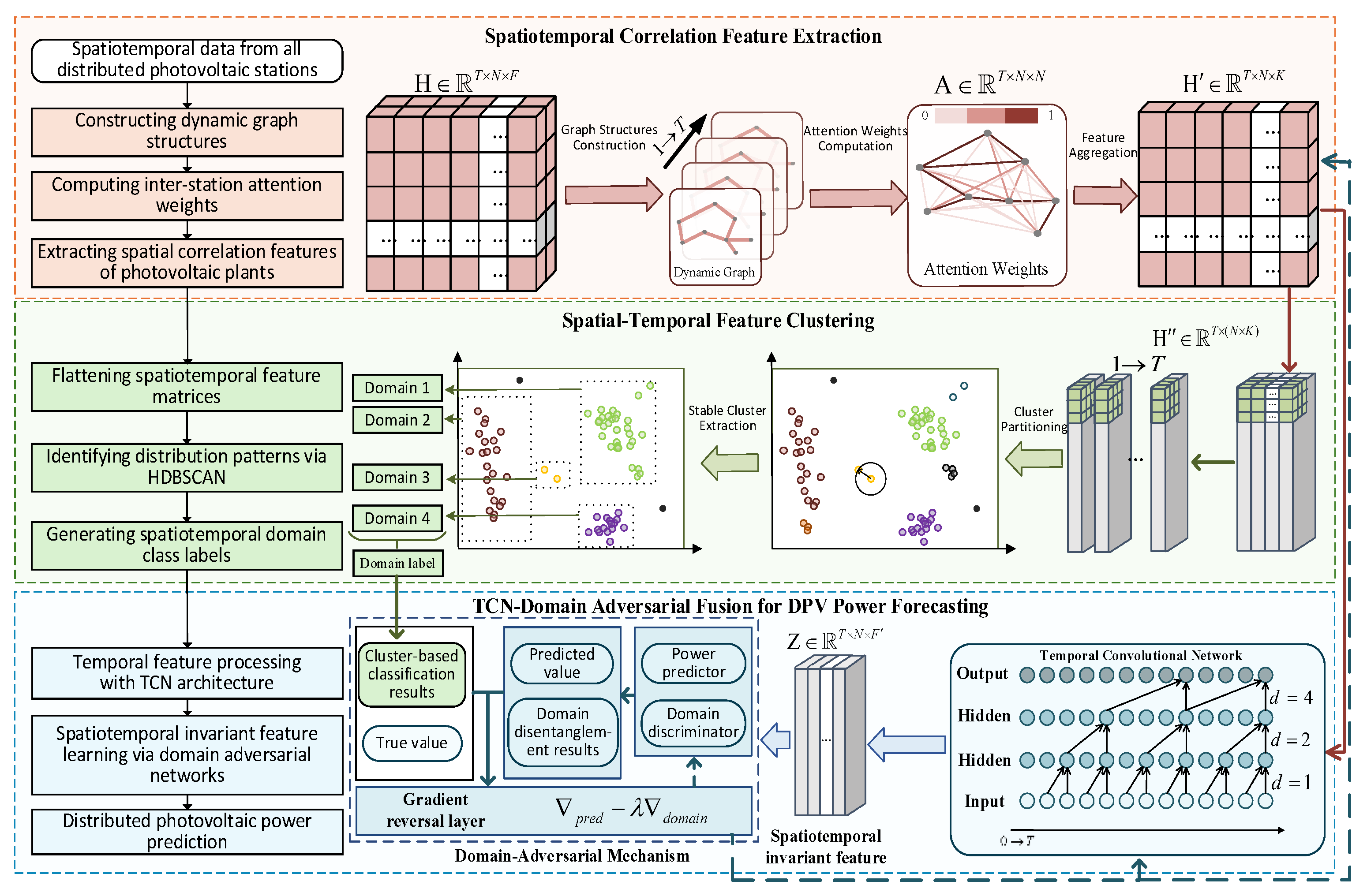
Figure 1. The architecture of the proposed model.
Electronics 14 04709 g001
Figure 2. Schematic diagram of the multi-head attention mechanism.
Electronics 14 04709 g002
Figure 3. Schematic diagram of TCN causal convolution.
Electronics 14 04709 g003
Figure 4. Schematic diagram of the domain-adversarial mechanism.
Electronics 14 04709 g004
Figure 5. Comparison of power output curves of adjacent PV power stations on the same day.
Electronics 14 04709 g005
Figure 6. Comparison of power output curves of the same power station under different weather conditions.
Electronics 14 04709 g006
Figure 7. NRMSE curves per step for different methods.
Electronics 14 04709 g007
Figure 8. NMAE curves per step for different methods.
Electronics 14 04709 g008
Table 1. Configuration of each forecasting method.
MethodForecasting ModelTemporal Distribution ShiftSpatial Distribution ShiftDomain-Adversarial Mechanism
M1GCNNoNoNo
M2GATNoYesNo
M3GATYesYesYes
M4GAT+TCNYesYesYes
Table 2. The NRMSE of Different Forecasting Methods.
M1M2M3M4
15 min0.06980.07050.06470.0652
1 h0.07810.07830.07630.0768
2 h0.08680.08630.08560.0851
3 h0.09210.09080.09010.0887
4 h0.10010.09540.09610.0943
Table 3. The NMAE of Different Forecasting Methods.
M1M2M3M4
15 min0.04000.03980.03660.0364
1 h0.04250.04240.04220.0418
2 h0.04570.04570.04580.0453
3 h0.04770.04760.04780.0474
4 h0.05340.05110.05040.0492
Table 4. Evaluation metrics of different weather conditions.
WeatherForecasting ScalesNRMSENMAE
M1M2M3M4M1M2M3M4
Sunny15 min0.04900.04840.03630.03670.03320.03240.02350.0227
1 h0.05050.05010.04290.04380.03170.03080.02700.0258
2 h0.05290.05230.05020.05030.03090.03030.02910.0286
3 h0.06180.05940.05930.05790.03560.03460.03380.0332
4 h0.07170.06980.07280.06660.04300.03980.04060.0376
Cloudy15 min0.07440.07450.06900.06960.04070.04080.03740.0366
1 h0.08760.08690.08550.08540.04470.04570.04480.0436
2 h0.09340.09370.09330.09320.04660.04840.04610.0463
3 h0.09710.09670.09520.09670.04790.05030.05080.0477
4 h0.10340.10100.10320.10240.05660.05510.05540.0550
Rainy15 min0.07180.07130.06960.06940.04120.04100.03970.0397
1 h0.07830.07730.08010.07910.04530.04450.04410.0442
2 h0.09070.08830.09120.08800.04890.04880.04900.0480
3 h0.09630.09160.09630.09070.05070.04950.05090.0493
4 h0.10510.09590.10640.09550.05740.05640.05420.0531
Disclaimer/Publisher’s Note: The statements, opinions and data contained in all publications are solely those of the individual author(s) and contributor(s) and not of MDPI and/or the editor(s). MDPI and/or the editor(s) disclaim responsibility for any injury to people or property resulting from any ideas, methods, instructions or products referred to in the content.