


Abstract
Wireless sensor networks (WSNs) have widespread applications in vital fields, including environmental surveillance, medical care, and smart urban settings. Nevertheless, the restricted battery capacity of sensor nodes renders energy consumption an ongoing hindrance, limiting both the performance and operational lifespan of a network. To mitigate this challenge, this study proposes an enhanced clustering and routing scheme, the Black-Kite Optimization–Time Of Arrival (BKA-TOA) algorithm, which jointly optimizes cluster head selection and data transmission. The proposed BKA-TOA integrates the bio-inspired Black-Kite Optimization (BKA) with relay selection based on the Time of Arrival (TOA) technique. A multidimensional fitness function is constructed by incorporating inter-node distance, energy variance, and cluster head distribution to achieve robust clustering, balanced energy consumption, and improved scalability. Extensive simulations conducted in Matlab R2024a are used to benchmark the proposed algorithm against Particle Swarm Optimization (PSO), Improved Ant Colony–minimum spanning tree (IACO-MST), and Energy-Efficient Uneven Clustering (EEUC). The experimental results indicate that BKA-TOA significantly reduces node mortality, improves residual energy preservation, and prolongs the operational lifetime of WSNs compared with competing algorithms.
1. Introduction
Wireless sensor networks (WSNs), as a key technological medium connecting the physical world with digital systems, have been widely applied in diverse scenarios, such as environmental monitoring, smart agriculture, underground pipeline maintenance, forest fire prevention, and medical surveillance. The common characteristic of these application scenarios is that sensor nodes are often deployed in areas with complex terrain, harsh environmental conditions, and limited human accessibility. For example, in ecological monitoring of remote mountainous areas, nodes must withstand extreme weather such as alternating high and low temperatures and strong storms; in urban underground utility tunnel monitoring, nodes must operate for long periods in dark, humid, electromagnetically noisy, and enclosed spaces; in forest fire early-warning systems, nodes are distributed in mountainous and forested regions with rugged terrain and poor accessibility [1].
In such scenarios, the core function of sensor nodes is to perform real-time acquisition, local preprocessing, and long-distance transmission of environmental information. The critical resource supporting these functions is the energy that is stored in the nodes’ built-in batteries. However, due to constraints from node miniaturization, deployment cost control, and portability requirements, the battery capacity of sensor nodes is typically limited. Manual replacement of batteries requires overcoming terrain obstacles and environmental restrictions, which not only makes operations difficult and labor- and time-intensive but may also cause secondary damage to the ecological environment or infrastructure of the monitored area. In addition, in certain extreme environments, approaching the nodes poses safety risks, making battery replacement practically infeasible.
More importantly, sensor nodes exhibit two distinct characteristics in terms of energy consumption: irreversibility and imbalance. Once the battery is exhausted, a node permanently loses its functionality. If a large number of nodes fail simultaneously, “sensing blind spots” will emerge in the monitored area, potentially paralyzing the entire network [2]. This imbalance stems from differences in nodes’ roles: cluster head nodes must handle data aggregation and forwarding, consuming energy much faster than regular nodes, which are only responsible for data collection. Furthermore, cluster heads located near the base station frequently forward data from other cluster heads, making them prone to the “hotspot” problem.
Therefore, during the operation of WSNs, how to achieve a dynamic balance of network energy load through rational clustering strategies, routing optimization, and resource scheduling; how to minimize unnecessary energy consumption while improving the efficiency and reliability of data transmission; and, ultimately, how to extend the overall network lifetime have become core challenges urgently requiring breakthroughs in current WSN research. Addressing this issue can not only cut down the deployment and upkeep costs of WSNs but also broaden their use in extreme environments and long-term monitoring cases. In this way, it offers crucial technical backing for the large-scale implementation of smart sensing and Internet of Things applications.
2. Basic Knowledge
2.1. Current State of Domestic and International Research
To date, extensive studies have been conducted by domestic and international scholars on the node energy consumption problem in WSNs, with numerous methods being proposed. Among them, swarm intelligence algorithms (such as Particle Swarm Optimization, PSO; Ant Colony Optimization, ACO; Artificial Bee Colony, ABC; and Whale Optimization Algorithm, WOA) have been widely applied in the design of clustering routing for WSNs due to their advantages of distributed optimization and strong robustness. They are mainly used to optimize cluster head selection, energy balancing, and path selection, thereby prolonging the network lifetime. For example, Reference [3] proposed a clustering routing algorithm combining PSO with fuzzy logic. Fuzzy logic is utilized to select the next-hop cluster head by considering factors such as residual energy, energy variance, and transmission distance, thereby achieving a balanced distribution of energy consumption and minimizing the overall network overhead. However, the multidimensional fuzzy logic decision-making process increases node computation costs, which limits the practicality of full-route decisions in resource-constrained WSN nodes. Reference [4] designed a cluster head selection and routing algorithm based on chaotic PSO. By initializing the PSO population with chaotic sequences, it avoids the premature convergence problem of traditional PSO. Nevertheless, the innovation of this algorithm is only focused on the cluster head selection stage, while the path transmission stage still relies on traditional methods, thus limiting the overall optimization effectiveness. Reference [5] combined a quantum-inspired Harris Hawk Optimizer (Q-HHO, a swarm intelligence algorithm) with Q-learning–deep reinforcement learning techniques for intelligent clustering and routing optimization in WSNs. However, the computational complexity of this algorithm is relatively high. Especially when running on resource-constrained WSN nodes, it may increase the initial energy consumption of nodes, making it unsuitable for low-power devices. Reference [6] improved the standard ACO algorithm through a multi-objective heuristic function, adaptive pheromone decay, and a load-balancing factor. However, its performance depends heavily on the effective configuration of multiple parameters. The parameter tuning process is complex, and under different network configurations, manual tuning may be required. Moreover, its robustness is insufficient in noisy or uncertain environments, where additional fuzzy logic is needed to handle uncertainties. Reference [7] proposed a reputation-based clustering routing algorithm for WSNs using an improved Bat Optimization–Fuzzy C-Means method. In the cluster head election stage, the algorithm dynamically selects cluster heads by considering different factors, such as node energy and distance. In the data transmission stage, it adopts a hybrid single- and multi-hop polling mechanism, utilizing the improved Bat Optimization algorithm to plan efficient and secure transmission routes, thereby reducing node energy consumption and improving routing security. However, this algorithm requires additional maintenance of reputation values, which increases communication and computation overhead, indirectly leading to higher energy consumption.
In summary, although the above methods have achieved certain results in optimizing cluster head election, balancing network load, and prolonging network lifetime, they still face challenges such as high computational costs, insufficient robustness, or limited application scenarios. To overcome these challenges, this paper introduces a clustering routing algorithm called BKA-TOA, which integrates the constrained Black-Winged Kite Optimization Algorithm (BKA) with the Time Of Arrival (TOA) technique. In the cluster head election stage, the improved BKA is employed to construct a fitness function combining node energy and distance, thereby selecting the optimal cluster heads. In the data transmission stage, TOA-based relay selection is introduced, considering metrics such as energy, distance, and packet loss rate to select the next-hop forwarding cluster head. This approach effectively mitigates the “hotspot” problem in WSN clustering routing (i.e., cluster heads near the base station consuming energy prematurely due to frequent data forwarding). Furthermore, a fallback mechanism is incorporated to ensure that each round of transmission has at least one cluster head, preventing complete network failure and enhancing algorithm robustness.
2.2. Algorithm Introduction
2.2.1. Black-Kite Algorithm (BKA)
The Black-Winged Kite Algorithm (BKA) is a novel swarm intelligence optimization algorithm inspired by the natural behavior of the black-winged kite, which alternates between “high-altitude circling search” and “diving predation” [8]. This process demonstrates the trade-off between broad exploration and fine-tuned exploitation. In mathematical modeling, the BKA achieves this alternation through position update formulas, fitness comparison, and dynamic balance factors, enabling it to locate the optimal solution within complex search spaces.
In wireless sensor networks (WSNs), reasonable cluster head selection can balance node energy consumption, reduce communication overhead, and extend network lifetime. Essentially, cluster head selection is an NP-hard combinatorial optimization problem, which requires considering multiple factors such as energy balancing, spatial distribution, communication distance, and dynamic adaptability. The BKA, with its balanced global search and local exploitation capability, flexibility of the fitness function (see Formula (1)), relatively low computational overhead, and strong robustness, is highly suitable for the cluster head selection problem in WSN clustering and routing. It not only enhances the efficiency and fairness of cluster head selection but also significantly reduces overall energy consumption and prolongs network lifetime, demonstrating clear advantages over traditional algorithms such as LEACH and PSO. Since LEACH is a classic routing protocol, and the other three algorithms used for performance comparison with the algorithm proposed in this paper (BKA-TOA) have all outperformed LEACH in the available literature after being compared with the LEACH protocol, therefore, in this experiment, we do not add an additional simulation experiment comparing LEACH with the BKA-TOA algorithm. In practical implementation, a combination of population initialization + energy constraints + distance constraints is adopted to ensure that the number of cluster heads remains reasonable (typically 3–8) and evenly distributed, thereby avoiding the “hotspot” problem. The initial population is generated through a hybrid method of the farthest-first strategy and energy-weighted ranking, which not only enhances spatial coverage but also prevents low-energy nodes from depleting prematurely [9].
2.2.2. Time of Arrival (TOA)
TOA (Time of Arrival) is a type of distance measurement and localization method based on the signal arrival time. The essence of the TOA algorithm lies in exploiting the linear relationship between the signal propagation time and distance (d = c × t, in which d is the distance, c is the signal propagation speed, and t is the arrival time). By measuring the arrival time at the base station or multiple reference nodes, the coordinates of the target node (e.g., sensor or cluster head) can be inferred.
In network routing optimization, TOA can be used not only for precise distance measurement but also as a mechanism for path optimization and relay selection [10]. Specifically, by estimating the transmission cost between nodes, TOA enables the dynamic selection of the optimal path, thereby improving the transmission efficiency. In wireless sensor networks (WSNs), clustering-based routing protocols usually consist of three stages: cluster head selection; cluster formation; and data transmission. TOA plays a crucial role in both the cluster formation and data transmission stages. In the clustering phase, TOA-based distance estimation helps nodes choose the nearest cluster head, leading to more balanced clusters and avoiding oversized clusters [11]. In the data transmission phase, TOA allows cluster heads to establish multi-hop relay paths. Rather than sending data directly to the base station across long distances, cluster heads transmit information through neighboring relay nodes using multi-hop communication. This approach balances energy usage across the network and greatly improves the overall energy efficiency and stability.
3. The Key Idea of Algorithm
3.1. System Model
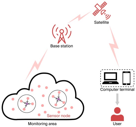
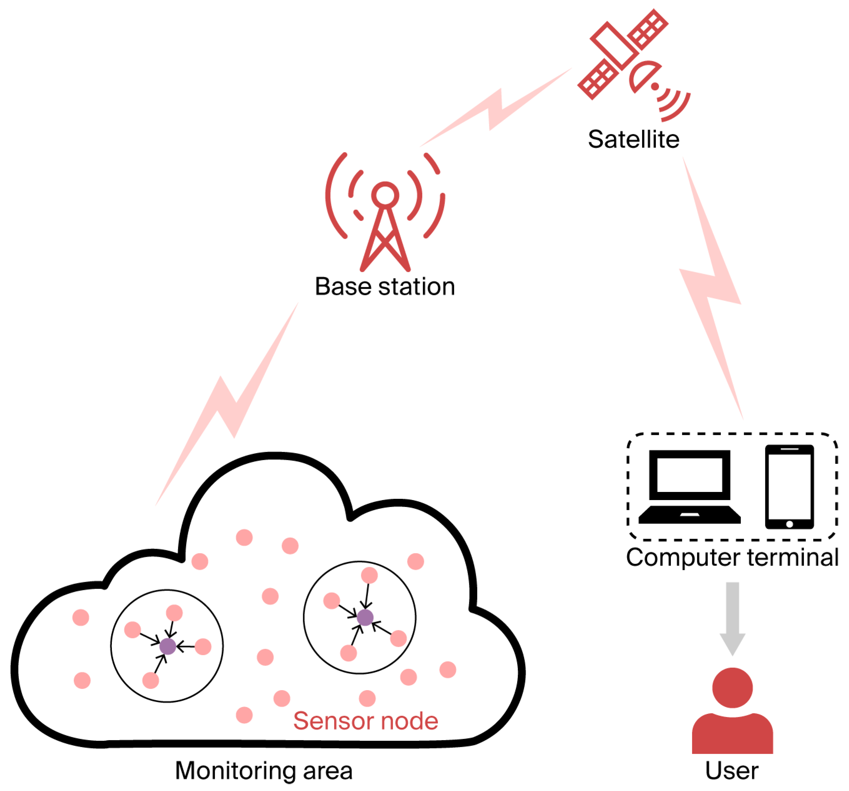
The topology of the wireless sensor network is shown in Figure 1. The nodes within the cluster will transmit the collected data to the cluster head node. After the cluster head node performs data fusion and processing, it transmits the data to the base station. The communication is ultimately carried out through the base station [12].
Figure 1.
The network model.
This paper constructs a static wireless sensor network (WSN) model, with the following specific assumptions:
- (1)
- The network is deployed in a two-dimensional monitoring area, consisting of one fixed base station and n static sensor nodes. The base station is located at the geometric center of the monitoring region and equipped with wireless power supply capability and storage resources, enabling it to directly communicate with all nodes [13]. The sensor nodes are randomly distributed within the monitoring area to collect environmental information, and their positions remain fixed after deployment.
- (2)
- All sensor nodes in the monitoring area are homogeneous, with identical initial energy, and they cannot be recharged. Once the energy is depleted, it cannot be replenished.
- (3)
- Each sensor node has a unique ID, which facilitates network identification and data transmission scheduling.
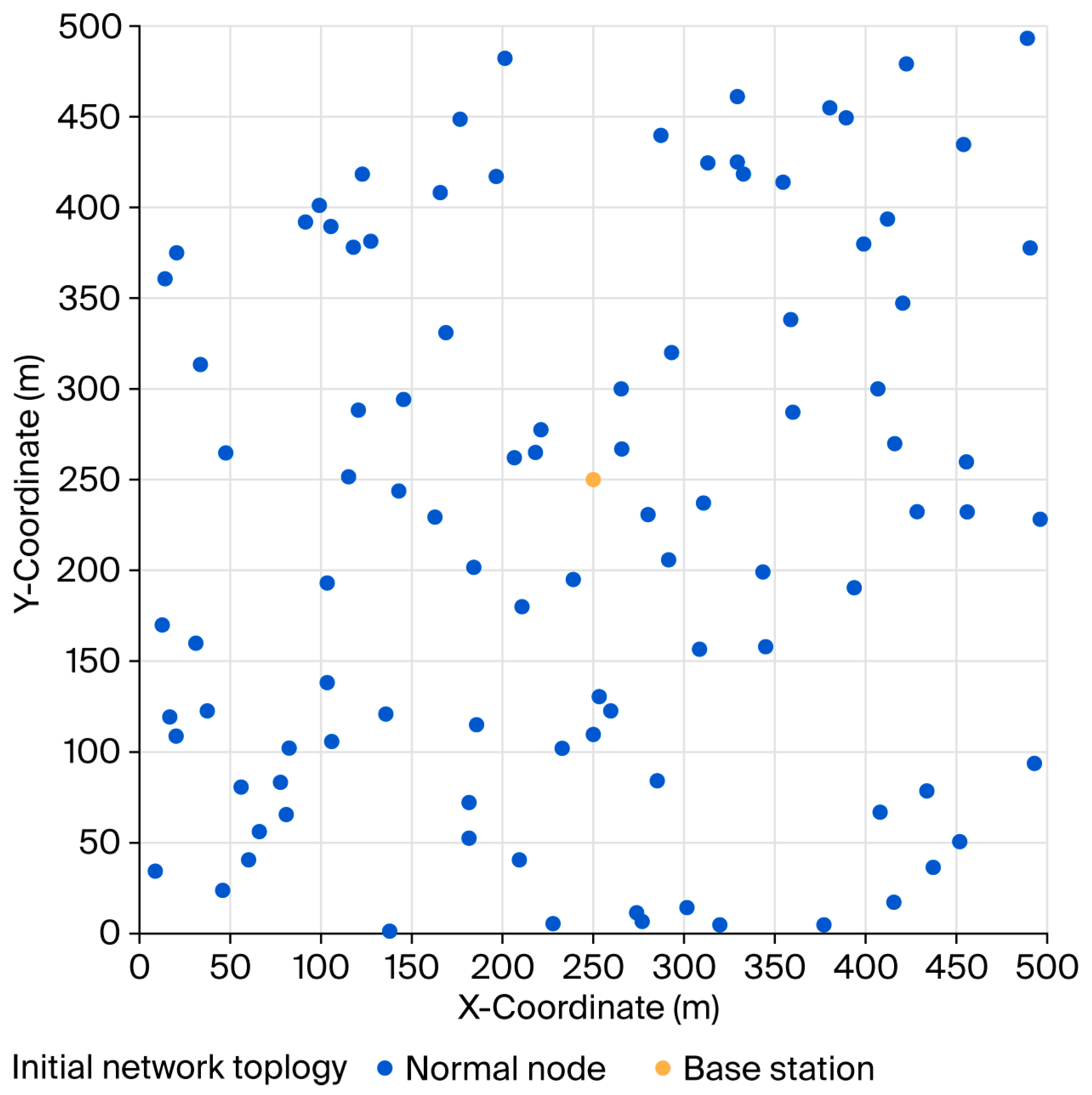
Figure 2.
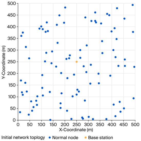
Initial network topology.
3.2. Energy Consumption Model
In this study, the classical first-order radio energy model is utilized to evaluate the energy consumption of nodes during data transmission and reception [14]. The energy expenditure for transmitting k bits of data is defined as follows:
When the transmission distance d between two communication nodes exceeds d0, the multipath fading channel model is applied. Conversely, if the transmission distance is less than d0, the free-space propagation model is utilized.
Here, represents the energy consumption of the node’s electronic circuitry (unit: J/bit), denotes the free-space channel attenuation coefficient (unit: J/(bit·m2)), denotes the multipath fading channel attenuation coefficient (unit: J/(bit·m4)), and d0 is the threshold transmission distance between nodes, defined as d0 = .
The energy consumption of a node receiving bits of data is only related to the operation of the circuitry and is given by Formula (3):
The radio energy model parameters are configured as follows: the electronic energy per bit for transmission and reception is set to Eelec = 50 nJ/bit, the data aggregation energy is EDA = 5 nJ/bit, the free-space amplifier coefficient is Efs = 10 pJ/(bit·m2), and the multipath fading coefficient is Emp = 0.0013 pJ/(bit·m4). The threshold distance between the free-space and multipath models is d0 = sqrt(Efs/Emp) ≈ 87.7 m. Each sensor transmits a 4000-bit data packet per round using a periodic traffic pattern over an ideal collision-free MAC layer. Random seeds are fixed to ensure reproducibility. The complete function hyperparameters will be elaborately explained in Section 3.3.
3.3. Algorithm Design
3.3.1. Cluster Head Selection Mechanism Based on the Black-Kite Optimization Algorithm
This paper adapts the BKA to cluster head selection in WSNs, transforming Black-Kites’ prey-seeking behavior into the selection of the optimal cluster heads [15]. The specific implementation process is as follows:
The uniform distribution of cluster heads is key to ensuring network energy balance and transmission efficiency. Therefore, during the population initialization phase, a combined strategy of “bio-inspired farthest-first selection + energy ranking + distance constraints” is adopted, ensuring that the number of cluster heads is within [CHmin, CHmax] = [3, 8] and the inter-cluster distance > minCHdist.
Before the algorithm enters the main loop, the population X (with dimensions pop × dim, where pop = 20 is the population size and dim = 1001 is the total number of nodes + 1, with each row representing a cluster head scheme) is generated [16]. By using a custom initialization function, it is ensured that the initial schemes are diverse and reasonable.
The farthest-first strategy selects the node that is farthest from the already chosen cluster heads as the new cluster head, maximizing the spatial coverage of cluster heads and avoiding the “hotspot” problem caused by excessive cluster head concentration. At the same time, an energy-weighted scoring mechanism is introduced to optimize the selection priority, given by Formula (4):
Here, is the distance between the candidate node and the already selected cluster heads, while represents the residual energy of the candidate node. By applying energy weighting, early node deaths are reduced, thereby extending the network lifetime.
The number of cluster heads is set within the range of [CHmin, CHmax] = [3, 8], and a minimum inter-cluster–head distance constraint is introduced by Formula (5):
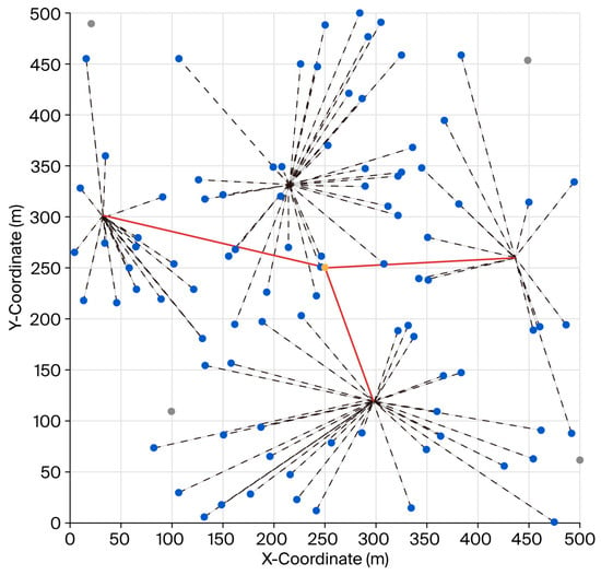
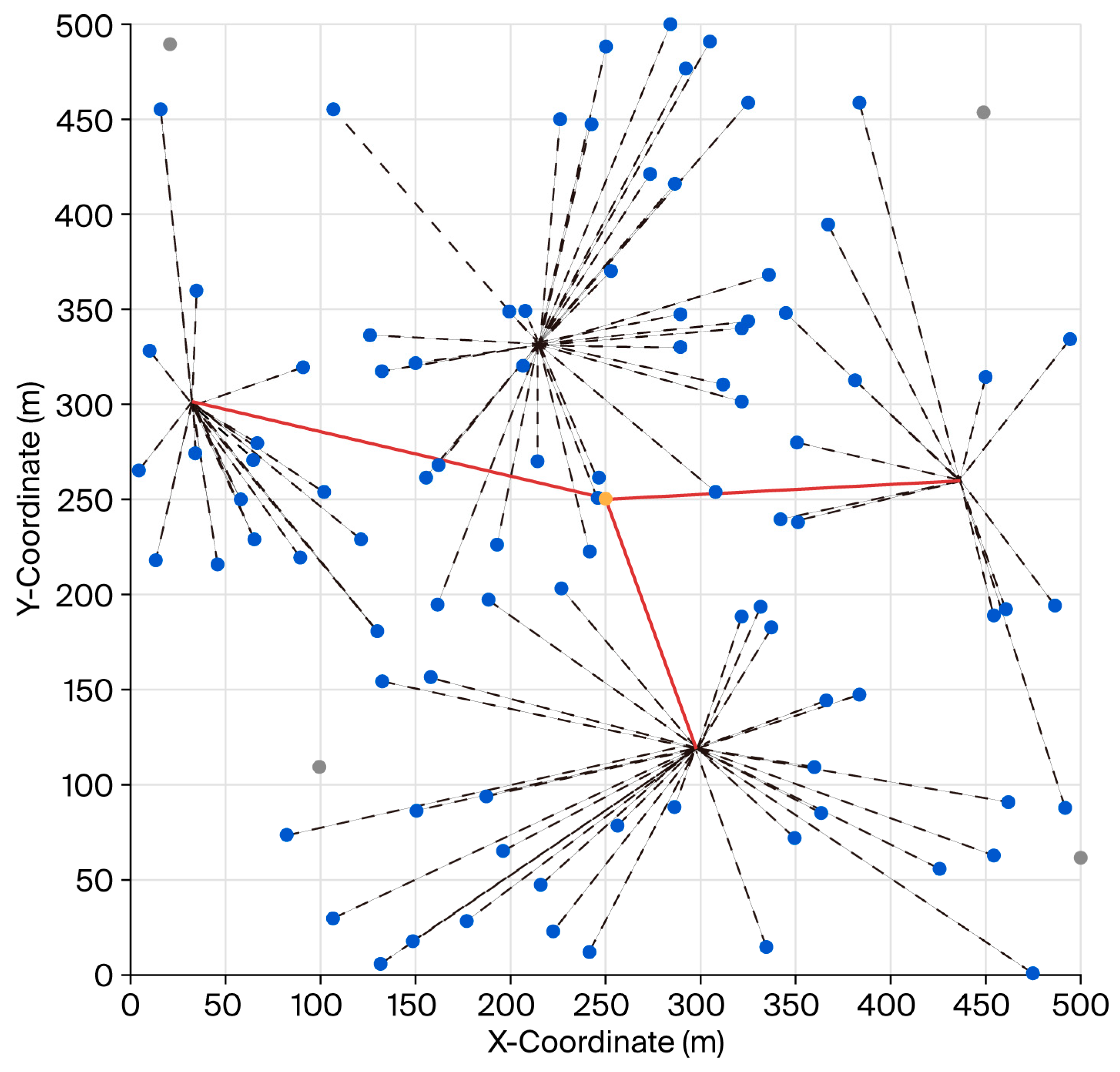
Here, avgNodeSpacing represents the average spacing between nodes. This value only reflects the average geometric distance of the nodes, but it cannot fully represent the ideal spatial distribution between cluster heads [17]. This is because, when selecting cluster heads in practice, multiple factors—such as the remaining energy of the nodes, the distance from the base station, and the size of the cluster—need to be considered. If the distance between cluster heads is too small, the system is prone to overlapping of cluster head areas, energy waste, and communication interference; if the distance between cluster heads is too large, it may lead to communication blind areas or excessive distance between nodes within the cluster. Therefore, in the existing literature and simulation studies, a regulating coefficient α ∈ [1.1, 1.5] is often introduced to amplify the average distance in order to better match the energy balance and spatial distribution [18]. Through a large number of experimental simulations and comparisons (refer to the research results of clustering algorithms such as BKA, PSO, and LEACH), when α = 1.2 is taken, the distribution of cluster heads in the network is the most balanced, and the network lifetime and energy utilization rate perform the best. For low-energy cluster heads whose distance is less than minCHdist, they are replaced with surviving nodes that are farther away, avoiding overlapping coverage and energy waste [19]. Figure 3 shows the network topology of the BKA-TOA algorithm at the 350th iteration, where the cluster heads are evenly distributed, without excessive concentration.
Figure 3.
BKA-TOA network topology—350th round.
3.3.2. Stage-Wise Position Update of BKA
The predation process of the Black-Kite is divided into two phases: “exploration (circling search)” and “exploitation (diving attack)”. During the exploration phase, Black-Kites perform large-scale whirlwind circling at long distances to search for prey. In the exploitation phase, the Black-Kite gradually reduces its whirlwind radius to quickly approach the prey, while the prey is disturbed due to fear [20]. Finally, when the algorithm attains the predefined maximum iteration limit or the convergence threshold, it enters the termination phase, where the prey is captured and the Black-Kite stops the whirlwind attack. This algorithm balances population diversity and optimal solution convergence through stage-wise position updates.
Exploration Phase (Circling Search)
This phase aims to expand the search range and maintain population diversity. The position update formula is as follows:
Here, denotes the position of the i-th individual during the t-th iteration, while indicates the best position identified by the population in the same iteration. The indices j and k correspond to two distinct randomly chosen individuals, and is a random value uniformly distributed within the range of [0, 1].
Exploitation Phase (Diving Attack)
This phase aims to narrow the search range, allowing individuals to approach the optimal solution. The position update formula is as follows:
Here, and are control parameters ( in this paper), and represents the average position of the population in the t-th iteration.
Stage Transition Mechanism
A transition factor, λ, is introduced to achieve a smooth transition from exploration to exploitation. λ increases linearly with the number of iterations (initial value: 0.1; final value: 0.9). The final rule for position updating is as follows:
If the updated individual position exceeds the boundary [LB, UB] (LB = 0 indicates non-cluster head; UB = 1 indicates cluster head), it is pulled back within the boundary range.
3.3.3. Algorithm Iteration and Optimal Cluster Head Selection
The algorithm runs for T iterations (as set according to the following scenarios: T = 1000 in Scenario 1; T = 2000 in Scenario 2). In each iteration, the Black-Kite algorithm performs 60 internal iterations. During the internal iterations, for each individual i = 1:pop, the position X (i,:) is updated according to the aforementioned rules, and the cluster head number and distance constraints are applied to ensure the feasibility of the solution [21]. The individual fitness is then calculated, and the individual best position, pBest, and population best position, Best_Pos, are updated. To further balance exploration and exploitation capabilities, a learning factor is introduced to optimize the position update, given by Formula (9):
Here, c1 = 2.5 (personal learning factor, enhancing local exploration); c2 = 3.0 (global learning factor, enhancing global convergence); and rand (1, dim) is a uniformly distributed random vector in [0, 1], adding stochastic variation to help the algorithm avoid premature convergence to local optima.
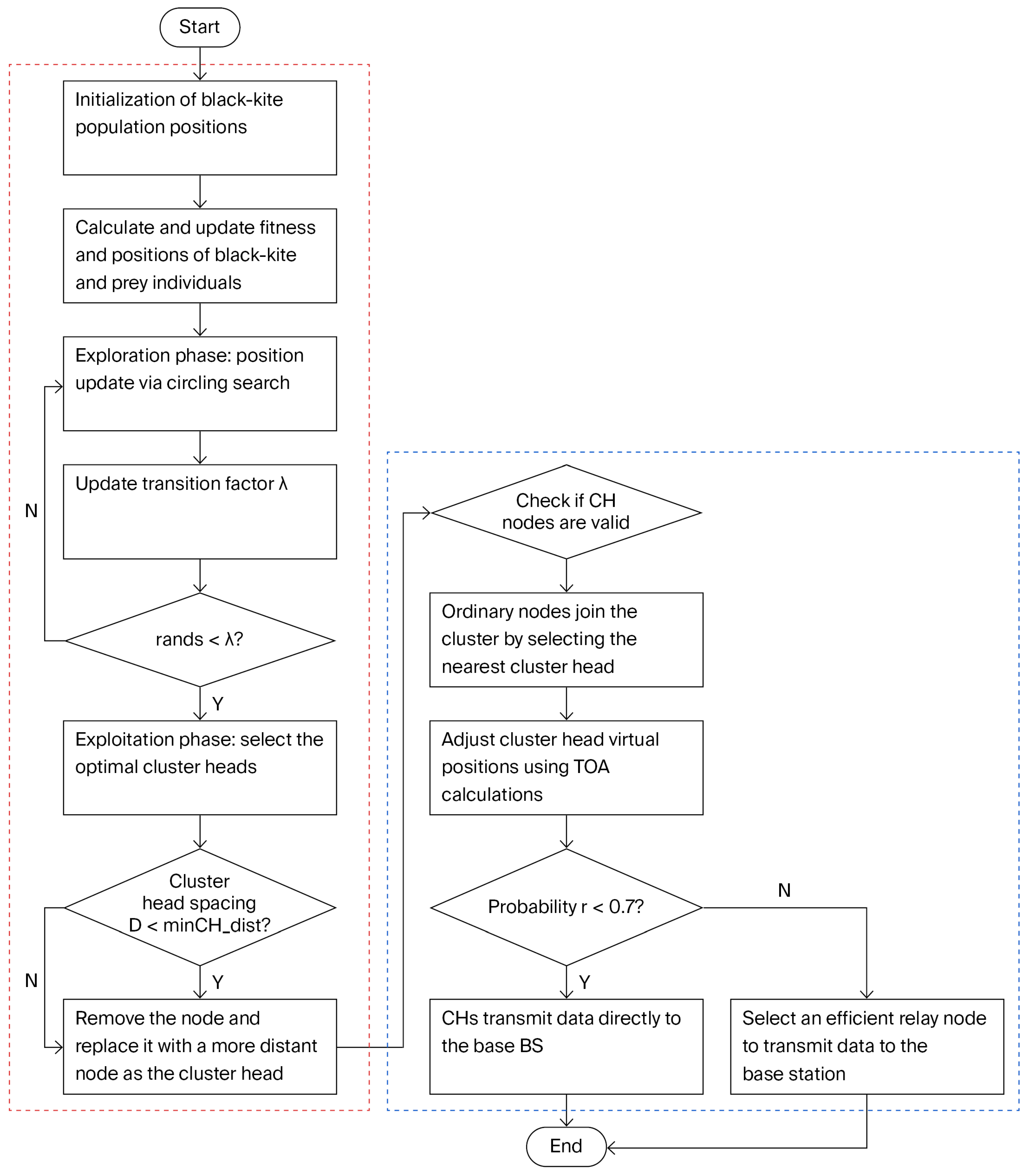
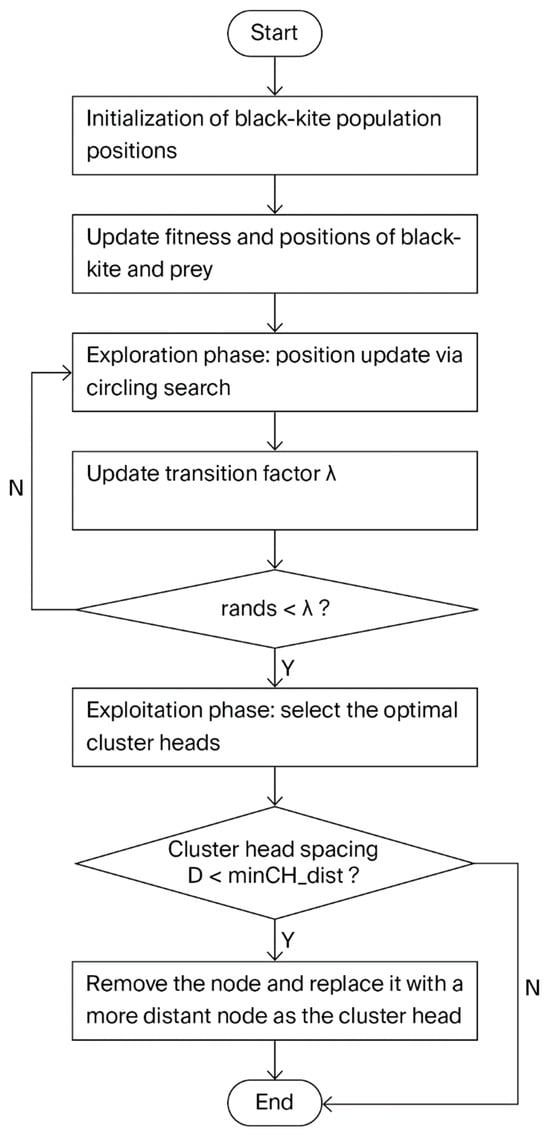
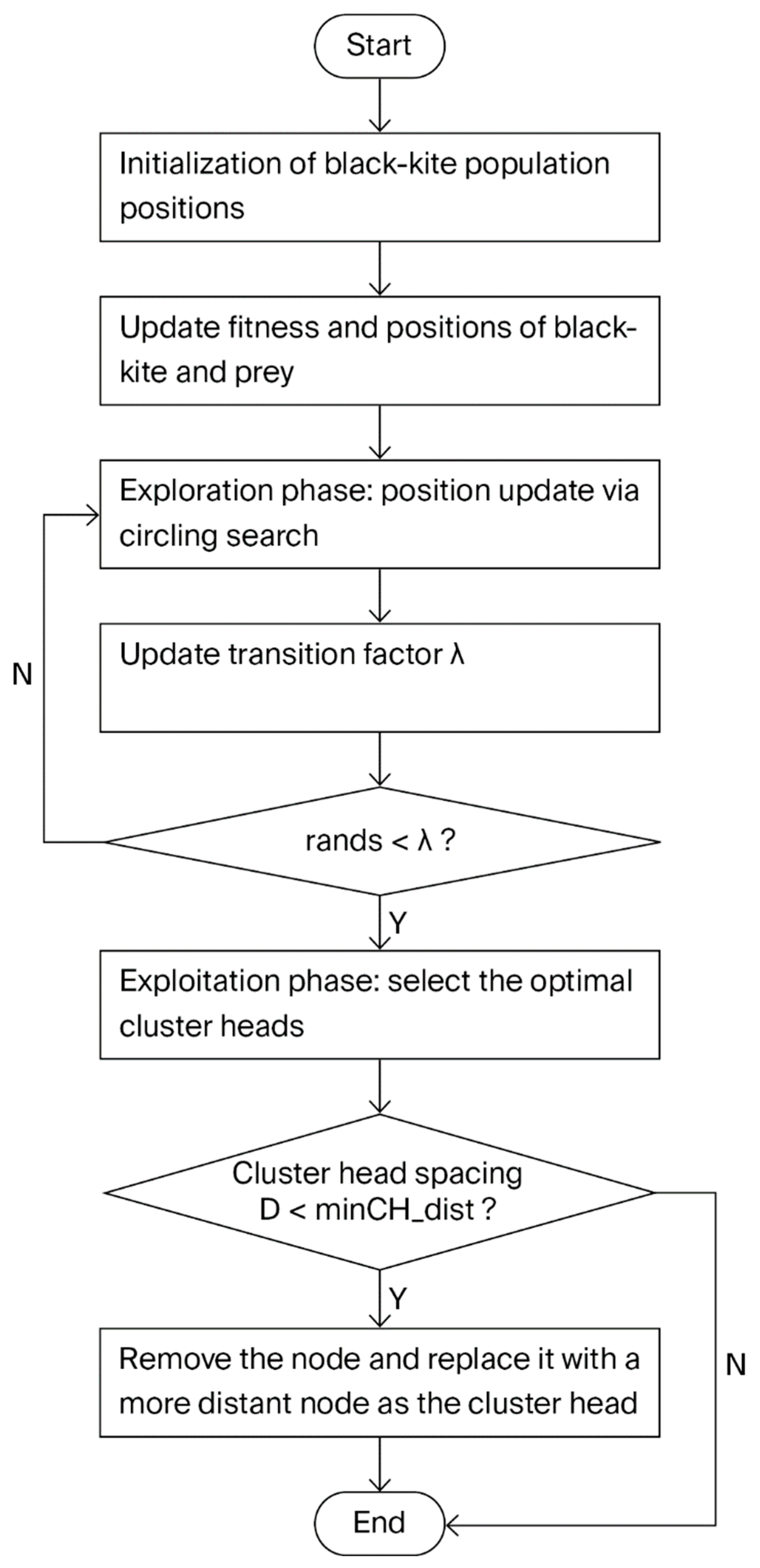
Through 60 internal iterations and parallel search by 20 individuals, the optimal cluster head scheme is quickly selected, improving the quality of cluster head selection and indirectly reducing network energy consumption [22]. The algorithm flow of BKA-based cluster head selection is shown in Figure 4.
Figure 4.
Flowchart of cluster head selection algorithm.
3.4. TOA-Based Clustering and Data Transmission Optimization Algorithm
In this paper, the Time of Arrival (TOA) technique is adopted for data transmission. Its working principle mainly consists of two key steps:
- (1)
- Iterative optimization of the “virtual positions” of cluster heads, which yields a set of optimized virtual positions for subsequent relay selection.
- (2)
- Relay cluster head selection based on these virtual positions. For each surviving cluster head, the distances to the virtual positions of other cluster heads are calculated.
Based on the computed distances, the cluster head determines whether to select a “relay cluster head”. According to the chosen relay path, the actual transmission distance is calculated, and combined with the wireless communication energy consumption model, the transmission energy consumption of the cluster head is determined to further update its remaining energy [23].
3.4.1. Preparation Phase
To avoid data transmission interruptions caused by cluster head energy depletion, a cluster head validity check and fallback mechanism are carried out before the TOA algorithm starts. First, the incoming cluster head vector, CH, is checked for validity (non-empty and contains at least one “1”):
At this point, if the selected cluster heads are invalid (node energy is 0), the fallback mechanism is triggered [24]. Subsequently, all active nodes in the network are traversed, and the node with the highest residual energy is designated as a temporary cluster head, as defined by the following formula:
Here, is the set of indices of surviving nodes, while represents the remaining energy of node i. At the same time, the population’s optimal cluster head position is updated:
Refreshing the surviving cluster heads can effectively avoid invalid computations, making the algorithm more adaptable to the energy-dynamic WSN environment. The fallback mechanism ensures that each transmission round has at least one cluster head, preventing complete network failure and enhancing algorithm robustness. With the fallback mechanism in place, situations where data links are interrupted due to the use of dead cluster heads, making data transmission impossible, are effectively avoided.
3.4.2. Intra-Cluster Data Transmission Phase
The core of intra-cluster data transmission is to reduce the transmission energy from ordinary nodes to cluster heads. A “dynamic clustering + energy-adaptive single-hop transmission” strategy is adopted.
During the intra-cluster clustering phase, the TOA algorithm does not use a static pre-clustering mode [25]. For each ordinary node (nonCH_idx), the Euclidean distance to all surviving cluster heads is calculated, and the nearest cluster head is selected as its belonging cluster, given by the formulae presented below.
Distance Calculation Formula:
Nearest Cluster Head Calculation:
targetCH = argminCH(dist)
Non-static pre-clustering allows clusters to form dynamically based on cluster head positions, avoiding the imbalance caused by fixed clusters. Using the nearest-distance principle reduces intra-cluster transmission distances, optimizes energy usage, and is also suitable for heterogeneous or mobile node scenarios [26].
For data transmission from ordinary nodes to cluster heads, this paper adopts an energy-adaptive single-hop transmission method. The data packet size is adjusted according to the remaining energy: low-energy nodes transmit smaller packets to prevent premature energy depletion and node death caused by transmitting large packets.
Dynamic Grouping L:L = packetLength × max (0.2, Enode/E0)
Here, packetLength denotes the basic packet size, Enode represents the residual energy of the ordinary node, and E0 refers to the node’s initial energy.
3.4.3. Inter-Cluster Data Transmission Phase
The core of inter-cluster data transmission lies in optimizing the routing path from cluster heads to the base station, thereby minimizing the energy consumption caused by long-distance transmissions [27]. By using TOA to simulate the signal propagation time, the virtual positions of cluster heads are adjusted to achieve efficient relay selection.
First, the virtual positions, pos, of all surviving cluster heads are initialized. A double-layer iterative adjustment strategy is adopted: “10 outer loops + inner loop for each cluster head.” The outer loop is repeated 10 times for progressive optimization, allowing the virtual positions to gradually approach the optimal path. In the inner loop, for each cluster head i, a random number r in [0, 1] is generated. If r < 0.7 (70% probability), the position moves closer to the base station, encouraging a globally optimal path. The formula is as follows:
Otherwise, another cluster head j is randomly selected (j = randi (pop_size)), and the virtual position moves closer to j, preventing cluster head isolation and enhancing local cooperation. The formula is as follows:
For each cluster head i, its virtual distance, dists, to other cluster heads is calculated, with the virtual distance formula being shown in Formula (19). The nearest cluster head is selected as the relay node, nextHop. If nextHop is valid (alive and with sufficient energy), cluster head i forwards data to the base station via nextHop; if nextHop is invalid, cluster head i transmits data directly to the base station. In this case, the actual minimum distance from minDist to nextHop is calculated, with the formula being shown in Formula (20). The actual transmission energy consumption is calculated according to the first-order model, avoiding energy waste caused by invalid relays.
The simulated distance serves as the basis for relay selection and is calculated as shown below.
Virtual distance calculation:
Actual transmission calculation:
If nextHop is valid,
Otherwise,
After the transmission is completed, the remaining energy, Slocal. E, of cluster head i is updated and fed back to the next iteration, forming a closed-loop optimization [28].
The TOA algorithm simulates TOA time differences through virtual adjustments, reducing invalid relays and lowering inter-cluster energy consumption. Combined with the 70% base station approach and 30% neighbor approach strategy, it ensures global path optimality while preventing cluster head isolation. This better supports dynamic WSNs and effectively extends their network lifetime. As the core of the data transmission component, TOA significantly improves the overall network transmission efficiency when integrated with network clustering.
4. Ablation Experiments
To verify the source of performance gain of the proposed BKA-TOA algorithm, this paper designs two sets of ablation experiments: the first group only uses the BKA algorithm for cluster head selection, and in the data transmission stage, nodes directly transmit data to their respective cluster heads, which then transmit the data to the base station; the second group only uses the TOA algorithm for route selection to make data transmission more energy-efficient. The third group is the BKA-TOA fusion algorithm proposed in this paper. The comparison and analysis are conducted from two dimensions: network lifetime and energy consumption.
The three experimental configurations have the same initial settings to ensure the fairness of the three experiments. Table 1 specifically shows the parameters of the initial settings:
Table 1.
Public parameter configuration.
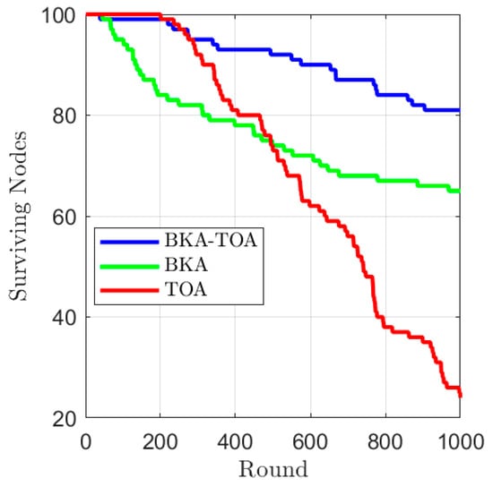
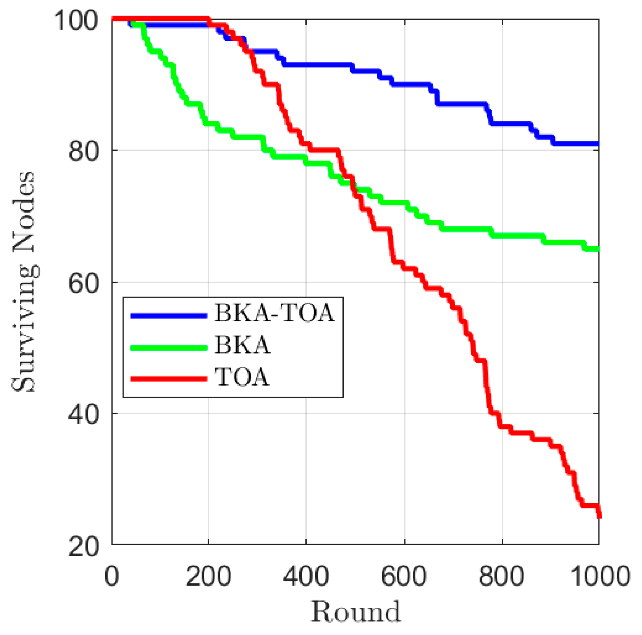
From the change in the number of surviving nodes (Figure 5), it can be seen that the BKA-TOA algorithm always maintains the largest number of surviving nodes throughout the simulation period. At the 1000th round, BKA-TOA still has over 80 nodes surviving, while the BKA algorithm has approximately 65 surviving nodes, and the TOA algorithm has only about 25 nodes remaining. This indicates that the BKA-TOA algorithm effectively balances the energy consumption of nodes through the collaborative mechanism of “BKA cluster head optimization + TOA route optimization”, significantly extending the survival time of nodes in the network.
Figure 5.
Comparison of surviving nodes in ablation experiments.
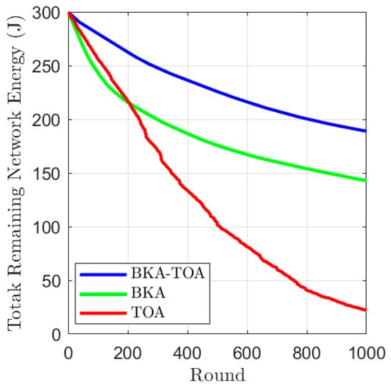
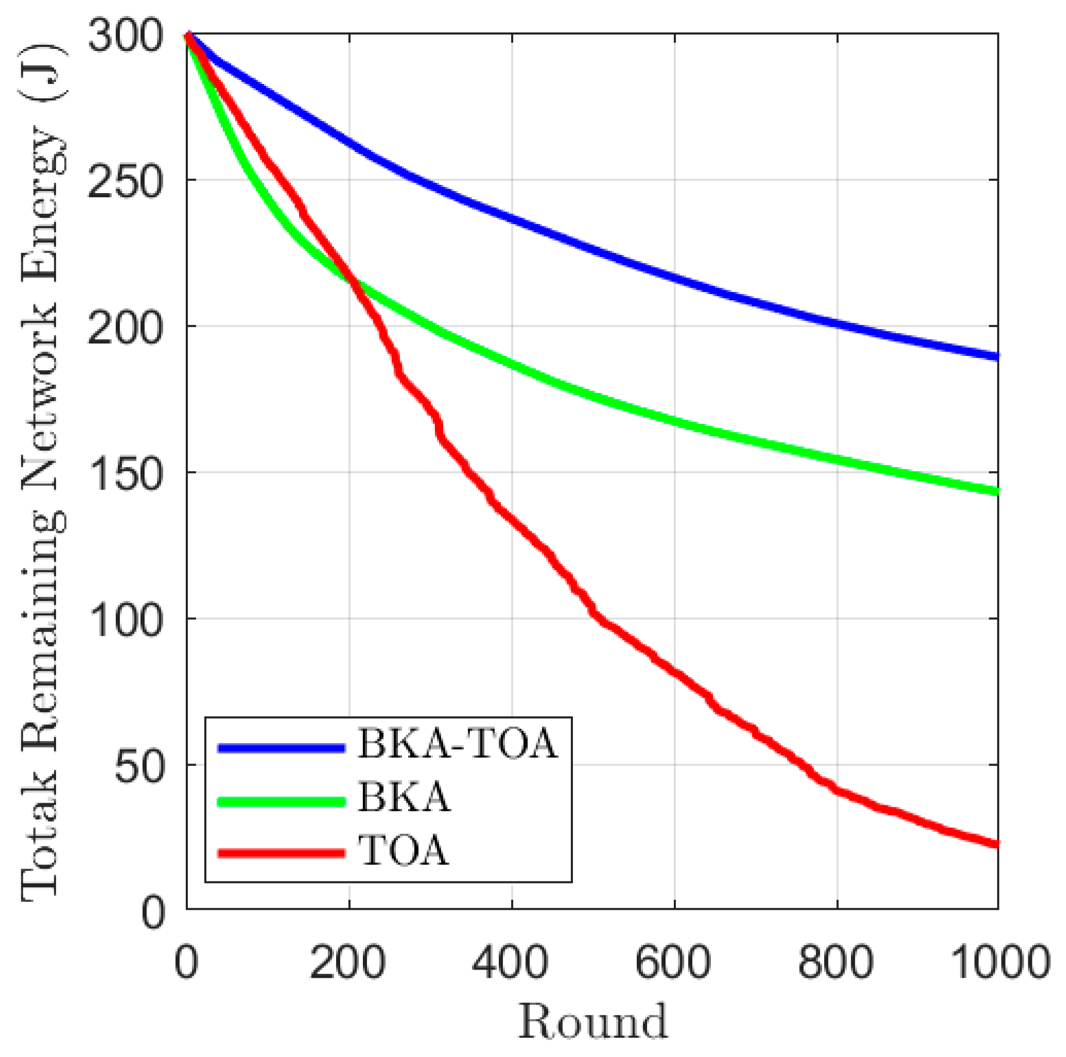
The change in the remaining energy of the entire network (Figure 6) further validates this conclusion. The BKA-TOA algorithm has the slowest energy consumption rate, with approximately 190 J of remaining energy in the entire network at the 1000th round; the BKA algorithm has about 145 J remaining, while the TOA algorithm has only about 30 J remaining. This shows that in the cluster head selection stage, BKA-TOA achieves a uniform distribution of cluster heads through the BKA algorithm, reducing the energy load on local nodes, and in the routing stage, it selects energy-efficient relay paths through the TOA algorithm, thereby optimizing the energy consumption efficiency of the entire network.
Figure 6.
Comparison of remaining network energy in the ablation experiment.
In conclusion, the results of the ablation experiments fully demonstrate that the synergy between BKA cluster head selection and TOA route optimization is the key to the performance improvement of the BKA-TOA algorithm. The combination of the two shows significant advantages in extending the network lifetime and reducing energy consumption.
5. Algorithm Implementation
In terms of algorithm design, the BKA improves the convergence speed of the optimal solution through stage-wise updates and learning factor adjustment; the energy-weighted and dynamic clustering mechanisms prevent individual nodes from depleting energy too quickly, ensuring strong energy balance; the fallback mechanism guarantees at least one valid cluster head in each round, preventing network collapse and enhancing robustness; and intra-cluster shortest-distance clustering combined with inter-cluster TOA-optimized paths reduces overall energy consumption and achieves high transmission efficiency.
The overall algorithm flowchart is shown in Figure 7.
In BKA-TOA, the overall calculation process of the algorithm mainly consists of three stages: population initialization, iterative optimization, and data transmission simulation [29]. Suppose that the number of nodes in the network is n, the population size is pop, the number of outer iterations is T, and the number of internal iterations in each round of the algorithm is numInnerIter.
In the initialization stage, the fitness calculation of each individual requires traversing all nodes to evaluate the distances from the cluster head to the base station and from the ordinary nodes. Its time complexity is O(pop × n). In the main optimization stage, the algorithm performs numInnerIter population update operations in each outer iteration round and calculates the fitness of all individuals in each update [30]. Since the fitness function involves distance calculations between nodes, the complexity is approximately O(n2), meaning that the overall time complexity of the main optimization stage can be expressed as O(T × numInnerIter × pop × n2).
From this, it can be seen that the fitness calculation and cluster head update process are the main computational bottlenecks of the algorithm [31].
The algorithm implementation is shown in Algorithm 1. In terms of space complexity, the algorithm mainly stores the population matrix (with a size of pop × n), node information structure, and distance matrix between nodes. Since the distance matrix occupies the largest amount of memory, it is O(n2), which is the main space cost of the algorithm. Therefore, the overall space complexity of the BKA-TOA algorithm is O(n2).
| Algorithm 1: BKA-TOA |
| // Inputs: |
| // pop: Population size, dim: Problem dimension (number of nodes), ub/lb: Upper/lower bounds of variables |
| // S_local: Set of sensor nodes, minCH/maxCH: Lower/upper bounds of cluster head (CH) count, minCHdist: Minimum distance between cluster heads |
| // fobj: Fitness function, T: Maximum number of iterations (simulation rounds), numInner: Number of inner iterations |
| // Levy_beta: Levy flight parameter, w/c1/c2: Adaptive weight and learning factors |
| // Outputs: |
| // Best_Pos: Optimal cluster head selection scheme, Best_Fitness: Optimal fitness value, Convergence_curve: Convergence curve |
In summary, the combination of BKA and TOA not only optimizes the cluster head selection process, forming a full-process “Select–Transmit” collaborative optimization framework that improves network structural balance, but also enhances data transmission by incorporating TOA-based positioning techniques into routing strategies, thus reducing energy consumption and ensuring reliability. This effectively lowers energy usage and extends the network lifetime [32]. The framework not only effectively prolongs the WSN’s lifetime but also demonstrates good scalability—when facing heterogeneous nodes, large-scale networks, or dynamic deployment environments, it can adapt to different scenarios by adjusting the cluster head number range, virtual position update parameters, and other settings, providing an efficient and practical optimization solution for real-world WSN applications.
The pseudo-code of this algorithm is as follows:
Figure 7.
Flowchart of the BKA-TOA algorithm.
6. Performance Simulation Analysis
To evaluate the performance advantages of the proposed algorithm, simulations of the BKA-TOA algorithm were conducted in the MATLAB R2024a environment. For comparison, classical algorithms, including PSO, EEUC, and IACO-MST, were incorporated to perform a comprehensive analysis [33].
Furthermore, to assess the scalability of the proposed algorithm, simulation experiments were conducted across multiple network scenarios using two key performance metrics: node mortality and residual network energy [34]. The parameters for each network scenario are summarized in Table 2 below.
Table 2.
The parameters of the different network scenarios.
The energy model parameters used in this experiment are shown in Table 3.
Table 3.
The energy model parameters.
6.1. Comparison of Network Node Deaths
In wireless sensor networks (WSNs), the definition of network lifetime is highly tied to the survival status of nodes. Since WSN nodes typically rely on batteries with limited capacity and are difficult to recharge or replace after deployment, the number of dead nodes directly determines the effective operational duration of the network [35]. When more than a threshold proportion of nodes in the network fail due to energy depletion, two critical issues arise: first, “holes” appear in data collection coverage, making it impossible to fully acquire information from the monitored area; second, data transmission links are broken, and even if some nodes remain functional, they cannot reliably forward data to the sink node. Therefore, the network lifetime has become a core indicator for measuring the performance of routing protocols, with its importance even surpassing that of traditional evaluation criteria such as transmission delay and data packet delivery rate.
To verify the performance of the proposed algorithm, experiments were conducted based on Network Scenario 1. The specific parameters of this scenario are as follows: the deployment area is a 500 m × 500 m square region, with 100 randomly distributed sensor nodes [36]. The sink node is fixed at the center of the region, all nodes are initialized with an energy of 4 J, the same wireless communication model is adopted for data transmission, and the iteration cycle is defined as the time required for a node to complete one round of “data collection and forwarding”.
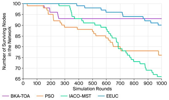
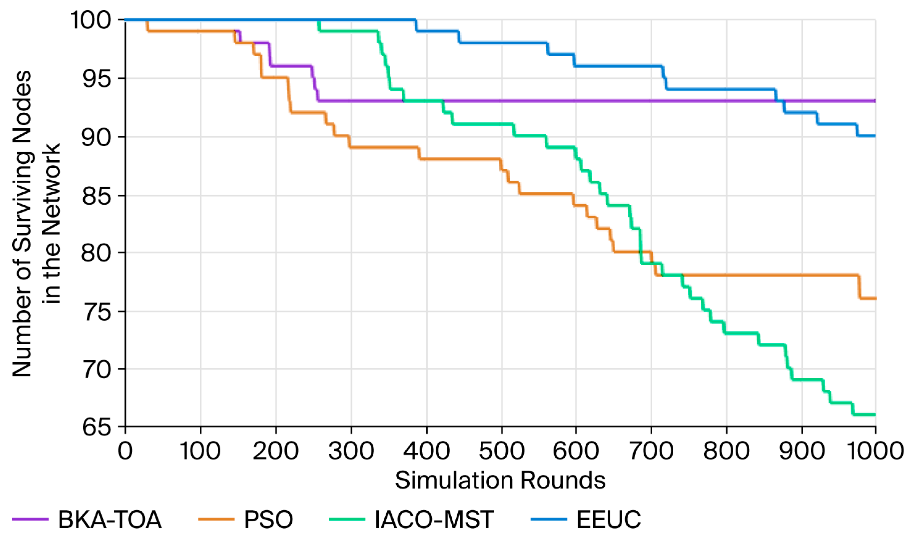
Figure 8 intuitively compares the variation trends of the number of surviving nodes of the four algorithms in this scenario. Three key phases can be observed from the curve trends: Initial Stable Phase (0–100 iterations): During this phase, the number of surviving nodes of the four algorithms (BKA-TOA, PSO, IACO-MST, and EEUC) remains 100. The network energy is in an initial balanced state, and no node death has occurred yet [37]. The energy consumption in this phase mainly comes from basic communication and intra-cluster data transmission, with a low overall energy consumption. Node Death Initiation Phase (approximately 100–800 iterations): As the number of simulation rounds increases, nodes of various algorithms begin to run out of energy. The PSO and IACO-MST algorithms see the first batch of node deaths after approximately 200 iterations, indicating certain imbalances in their energy allocation and routing strategies in the early stage. In contrast, the BKA-TOA and EEUC algorithms exhibit better energy balance, with a significantly delayed initiation of node death [38]. Among them, the EEUC algorithm experiences the first node death after approximately the 850th iteration, while the BKA-TOA algorithm starts to exhibit node deaths slightly earlier than EEUC, around the 820th iteration, representing a difference of about 30 iterations between the two. Late Attenuation Phase (800–1000 iterations): In this phase, the difference in the number of surviving nodes among different algorithms gradually widens. The curves of PSO and IACO-MST decline sharply, with a fast rate of node energy consumption, indicating imbalanced energy allocation during the late-stage data aggregation and routing phases. Although the EEUC algorithm performs well in the early stage, it experiences concentrated node deaths after the 900th iteration, leading to a sharp drop in the number of surviving nodes [39]. In comparison, the BKA-TOA algorithm demonstrates optimal energy balance and network robustness throughout the entire simulation process. It has the slowest node death rate and a gentle curve decline. Finally, after 1000 iterations, BKA-TOA still had 90 nodes remaining, with a survival rate of 90%; the survival rate of EEUC was 70%, that of IACO-MST was 68%, and that of PSO was the lowest (about 65%). The survival rate of BKA-TOA was 25 percentage points higher than that of PSO, 20 percentage points higher than that of EEUC, and 22 percentage points higher than that of IACO-MST.
Figure 8.
Number of surviving nodes in the network in Scenario 1.
In summary, the BKA-TOA algorithm exhibits optimal performance in terms of node energy balance and network lifetime. By dynamically adjusting its cluster head selection and routing path planning, it effectively delays the initiation of node death and improves the overall stability and survival cycle of the network. The late-stage advantage of the BKA-TOA algorithm in the number of surviving nodes essentially stems from its adaptive design for energy-constrained environments, which can be specifically attributed to two core mechanisms: Dynamic Routing Optimization: Unlike the EEUC algorithm, which adopts fixed cluster head election and routing paths, the BKA-TOA algorithm dynamically adjusts data forwarding paths based on the real-time remaining energy of each node, the distance to neighboring nodes, and data transmission priority. This avoids concentrating a large number of transmission tasks on a few nodes and achieves global balance in energy consumption. TOA Localization-Assisted Energy Consumption Control: The algorithm integrates Time of Arrival (TOA) localization technology, which can accurately calculate the actual communication distance between nodes and select the optimal transmission power. It reduces the transmission power to save energy during short-distance communication and replaces single-hop high-power transmission with multi-hop forwarding during long-distance transmission, thereby further reducing unnecessary energy loss. This design causes the BKA-TOA algorithm to require a small amount of additional energy consumption due to routing adjustments in the early stage (resulting in a slightly earlier initiation of node death). However, in the long run, its energy allocation balance is significantly superior to that of the EEUC algorithm, ultimately achieving an increase in the number of surviving nodes in the network and an extension of the network lifetime.
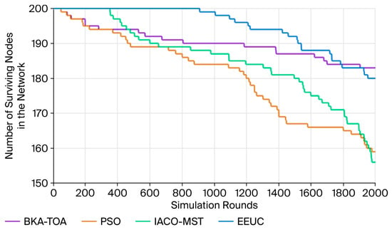
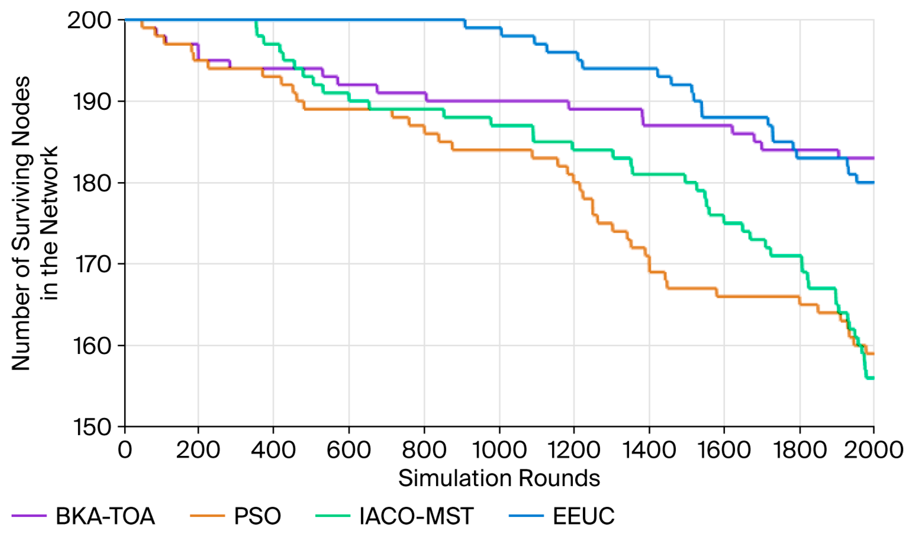
Experiments were conducted based on Network Scenario 2. The specific parameters of this scenario are as follows: the deployment area is an 800 m × 800 m square region, with 200 randomly distributed sensor nodes. The sink node is fixed at the center of the region, all nodes are initialized with an initial energy of 5 J, the same wireless communication model is adopted for data transmission, and the iteration cycle is defined as the time required for a node to complete one round of “data collection–forwarding”. Figure 9 intuitively compares the variation trends for the number of surviving nodes of the four algorithms in this scenario. Three key phases can be observed from the curve trends: Initial Stable Phase (0–200 iterations): During this phase, the number of surviving nodes of the four algorithms (BKA-TOA, PSO, IACO-MST, and EEUC) remains 200. This indicates that the network energy distribution is balanced in the initial stage, and the energy consumption difference among nodes is small. Due to the small amount of data and short communication distance, energy consumption is mainly concentrated in the processes of cluster head broadcasting and initial routing establishment, and no node death has occurred yet. Node Death Initiation Phase (approximately 200–1200 iterations): As the number of iterations increases, some algorithms gradually experience node death. The curves of the PSO and IACO-MST algorithms start to decline after approximately 400 iterations, indicating imbalances in their energy allocation and cluster head selection, which cause some nodes to run out of energy early. In contrast, both the EEUC and BKA-TOA algorithms can maintain the survival of all nodes for a longer period. Among them, the EEUC algorithm experiences the first node death at approximately the 1100th iteration, while the BKA-TOA algorithm experiences node death slightly earlier, around the 1000th iteration, representing a gap of about 100 iterations between the two. Late Attenuation Phase (1200–2000 iterations): In this phase, the performance differences between different algorithms gradually become apparent. The curves of PSO and IACO-MST decline significantly, with accelerated node death speed, imbalanced energy consumption, and weak network robustness [40]. The EEUC algorithm experiences concentrated node death after the 1500th iteration, indicating that its energy control mechanism becomes imbalanced in the mid-to-late stage. However, the BKA-TOA algorithm effectively suppresses the excessive energy consumption of nodes through dynamic routing optimization and energy-adaptive data transmission strategies, resulting in its curve exhibiting the gentlest decline. After 2000 iterations, the survival rate of BKA-TOA was 92.5% (185 nodes), while that of EEUC was 86% (172 nodes), IACO-MST was 82.5% (165 nodes), and PSO was 80% (160 nodes). The survival rate of BKA-TOA was 12.5 percentage points higher than that of PSO, 10 percentage points higher than that of IACO-MST, and 6.5 percentage points higher than that of EEUC. The BKA-TOA algorithm still exhibits strong stability and energy balance in Scenario 2, where the number of nodes is increased and the network scale is expanded.
Figure 9.
Number of surviving nodes in the network in Scenario 2.
6.2. Comparison of Network Residual Energy
Network residual energy represents the cumulative remaining energy of all nodes within a wireless sensor network and serves as a key indicator for evaluating overall energy utilization and depletion rate [41]. It directly reflects the effectiveness of a routing protocol in managing energy consumption across the entire network, thereby determining the network’s operational lifetime.
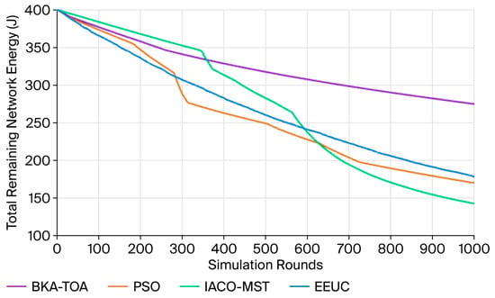
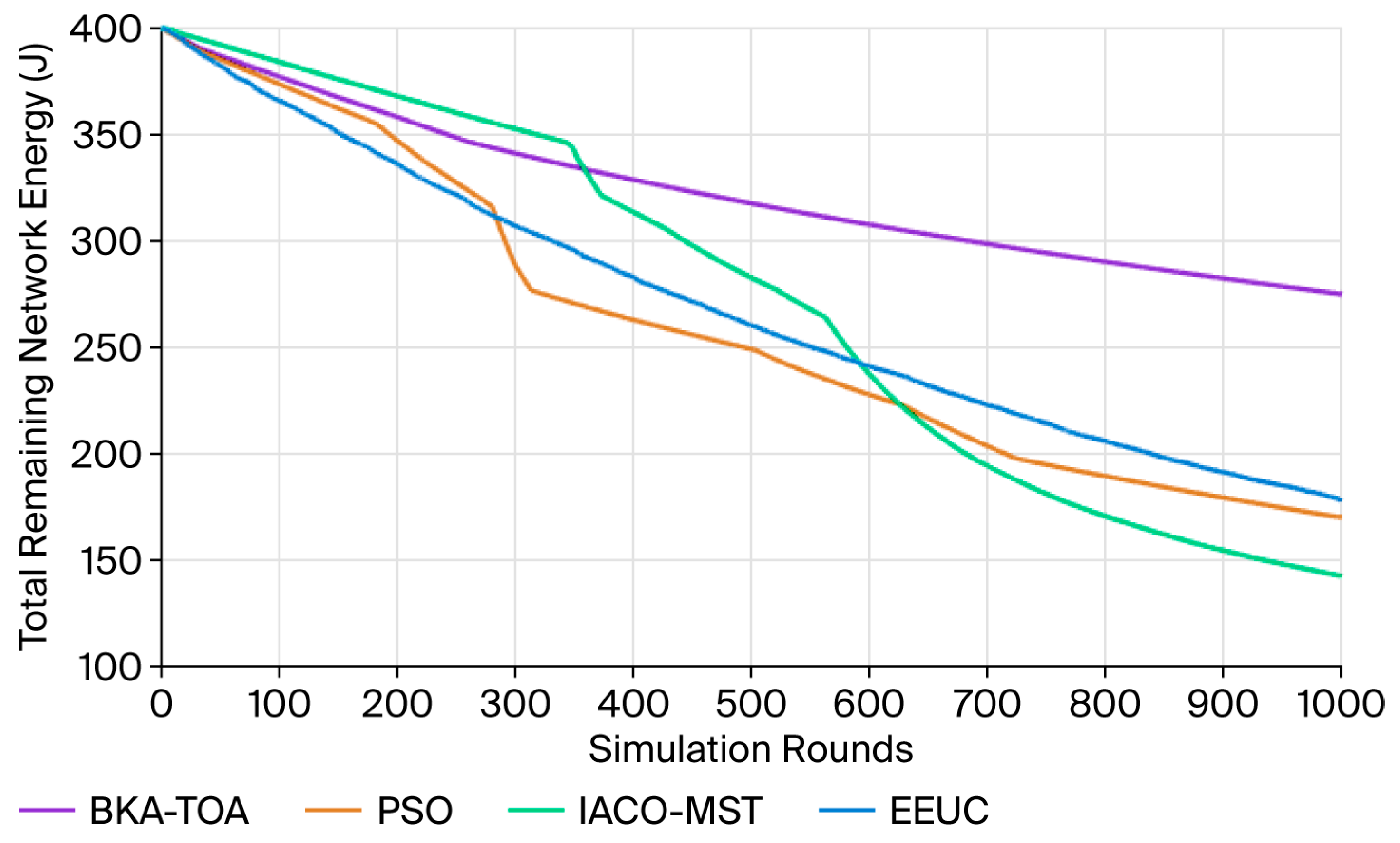
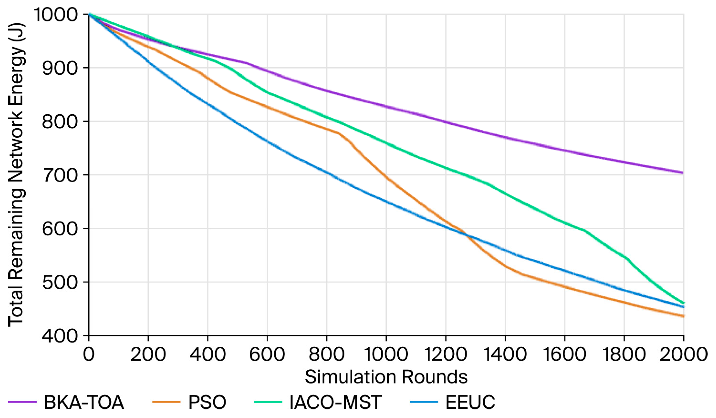
Figure 10 illustrates the trend of network energy variation with increasing iterations across the four algorithms in Scenario 1. With each node initialized at an energy level of E0 = 4, after 1000 rounds, the remaining energy of BKA-TOA is approximately 60% of the initial value, that of EEUC is about 45%, for IACO-MST, it is approximately 40%, and that of PSO is about 35%. The energy retention rate of BKA-TOA is 25 percentage points higher than that of PSO and 20 percentage points higher than that of IACO-MST. These results show that after 1000 iterations, the BKA-TOA algorithm retains a significantly higher residual energy than PSO, EEUC, and IACO-MST, demonstrating its superior efficiency in conserving energy and extending the network operation time.
Figure 10.
Total remaining network energy in Scenario 1.
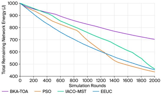
Figure 11 shows the total network residual energy versus the number of algorithm iterations for the four algorithms in Scenario 2 [42]. All nodes initially have E0 = 5. After 2000 iterations, the remaining energy of BKA-TOA was approximately 75% of the initial value, while for EEUC, it was about 62%, that of IACO-MST was about 58%, and that of PSO was about 55%. The energy retention rate of BKA-TOA was 20 percentage points higher than that of PSO and 17 percentage points higher than that of IACO-MST. The proposed BKA-TOA algorithm not only achieves a higher total network residual energy at the end of the run than the other three algorithms, it also consumes energy more slowly during the process. This is because, in the inter-cluster communication phase, BKA-TOA uses virtual adjustments to simulate TOA time differences, reducing invalid relays and selecting efficient paths, which lowers inter-cluster energy consumption. As a result, nodes retain more residual energy, effectively extending the overall network lifetime.
Figure 11.
Total remaining network energy in Scenario 2.
6.3. Average Transmission Distance
The energy of WSN nodes is mainly consumed by data transmission, and the transmission energy consumption has a “nonlinear positive correlation” with distance [43]. For example, in the free-space propagation model, energy consumption is proportional to the square of the distance; in the multipath fading model, it is proportional to the fourth power of the distance. The transmission distance is an important indirect indicator for measuring the real-time performance and integrity of data transmission, which directly affects a network’s quality of service (QoS). Excessively long transmission distances will increase signal propagation time and may also lead to an increase in retransmission times due to path loss, thereby prolonging data transmission delay. The core of clustering routing is to maintain the network topology through reasonable clustering and routing, and the variation trend of the transmission distance can directly reflect the dynamic state of the topology.
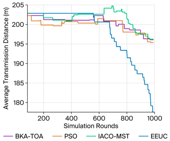
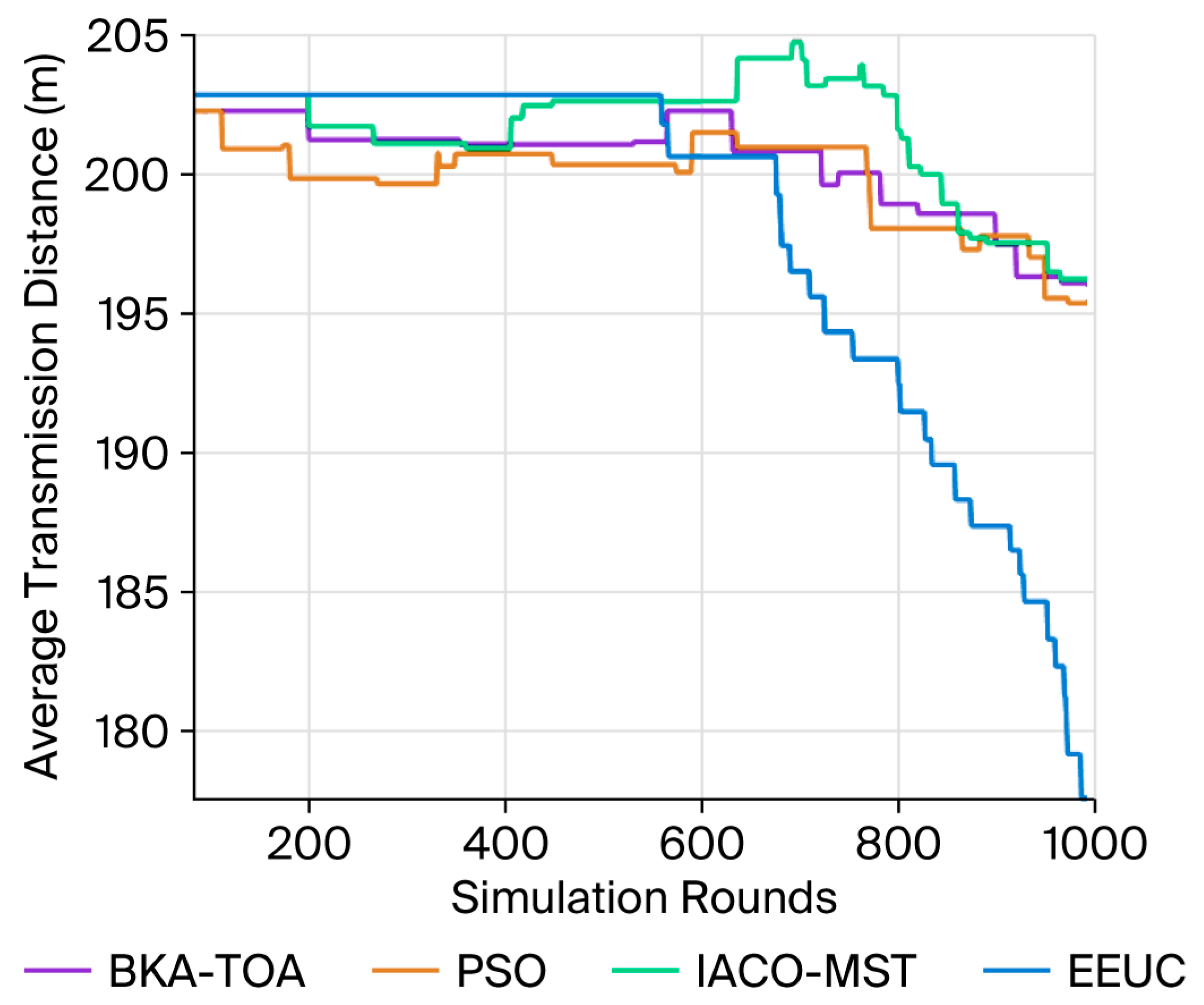
Figure 12 illustrates the variation in the average transmission distance of the four algorithms in Scenario 1 over the course of the simulation. The observed trends can be divided into three distinct phases, corresponding to different stages of network evolution. At the beginning of the simulation, all four algorithms maintain an average transmission distance between 200 m and 205 m, showing minimal fluctuation. During this period, the network structure remains stable, and energy consumption across nodes is evenly distributed. Since all nodes have sufficient residual energy, the cluster head selection and routing paths remain steady, resulting in consistent transmission distances. As some nodes begin to deplete their energy, the cluster structure and routing topology gradually adjust. The EEUC algorithm exhibits an early decline in transmission distance after around 600 rounds, indicating unstable clustering and frequent reconfiguration due to early cluster head failures. This leads to shorter but less energy-efficient communication paths. The IACO-MST algorithm shows noticeable fluctuations between 500 and 700 rounds, suggesting that its minimum spanning tree-based routing undergoes frequent adjustments, balancing between path optimality and energy balance. Both PSO (red) and BKA-TOA (blue) maintain relatively stable transmission distances, with BKA-TOA showing slightly higher consistency. This stability implies that BKA-TOA effectively balances routing efficiency and energy consumption through its adaptive optimization process. In the later stage, as the number of dead nodes increases, the network topology becomes less connected, leading to a general decline in average transmission distance. The EEUC algorithm experiences the sharpest drop, falling below 180 m, indicating severe topology fragmentation and localized energy depletion. IACO-MST demonstrates moderate instability as the routing tree deteriorates with node failures. PSO maintains a steady performance at approximately 195 m, showing moderate robustness. BKA-TOA maintains a smoother downward trend, with a final average transmission distance of around 198 m, indicating stable performance and minimal oscillation throughout the simulation.
Figure 12.
Average transmission distance in Scenario 1.
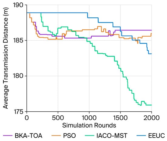
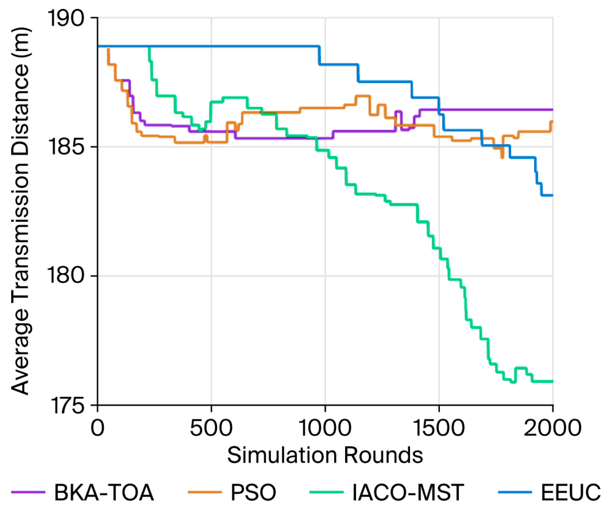
Figure 13 presents the variation in the average transmission distance of four algorithms in Scenario 2 throughout 2000 simulation rounds. The trend reflects the network’s routing adaptability and stability under continuous energy consumption and node failures.
Figure 13.
Average transmission distance in Scenario 2.
At the start of the simulation, all four algorithms maintain similar transmission distances within the range of 185–188 m, showing minimal fluctuation. This indicates that all cluster heads are effectively distributed, and the network topology remains balanced. During this phase, energy consumption across nodes is relatively uniform, and no significant structural changes occur. As energy consumption progresses, differences among the algorithms become apparent: The EEUC algorithm experiences minor oscillations around 500 rounds, reflecting unstable clustering caused by uneven energy distribution. Despite initially shorter distances, its routing paths become increasingly unstable as low-energy nodes start to fail. The IACO-MST algorithm begins to show a gradual decline in average transmission distance after approximately 700 rounds [44]. This trend suggests that its minimum spanning tree-based routing structure becomes fragmented due to node deaths, resulting in reduced path lengths but less efficient energy utilization. Both PSO and BKA-TOA maintain steady transmission distances throughout this phase. The BKA-TOA algorithm, in particular, benefits from adaptive optimization of relay nodes based on TOA metrics and residual energy, which helps preserve a stable routing structure, even as nodes deplete energy. In the later phase of the simulation, the divergence between algorithms becomes more pronounced. The IACO-MST algorithm’s transmission distance drops sharply below 180 m, indicating severe fragmentation of the network and poor data delivery continuity. EEUC also exhibits a noticeable downward trend, reflecting increased local transmissions due to early cluster head failures. In contrast, PSO and BKA-TOA maintain relatively stable and longer average transmission distances (around 185 m), implying that these methods sustain inter-cluster connectivity for a longer duration. Notably, BKA-TOA achieves the smoothest decline curve, demonstrating superior robustness against topology fragmentation and network imbalance.
Overall, the BKA-TOA algorithm shows the most stable and energy-balanced transmission behavior throughout the simulation [45]. Its TOA-based adaptive routing and bio-inspired optimization strategy allow it to dynamically adjust communication paths according to node energy levels and spatial distribution. This not only maintains moderate transmission distances but also prevents excessive reliance on specific relay nodes, effectively mitigating localized energy depletion. Consequently, BKA-TOA outperforms the classical PSO, IACO-MST, and EEUC algorithms in maintaining routing stability, load balance, and energy efficiency, ultimately contributing to a prolonged network lifetime [46].
7. Conclusions and Future Outlook
In wireless sensor networks (WSNs), where energy is limited and network lifetime is crucial, this paper proposes an innovative approach that combines the Black-Kite Algorithm (BKA) with a Time-of-Arrival (TOA)-based node localization and routing optimization mechanism. This hybrid strategy aims to address the problems of inefficient cluster head selection and difficult optimization of energy-aware data transmission, thereby significantly extending the operational lifetime of WSNs. The proposed BKA is inspired by the predation behavior of Black-Kites in nature and uses swarm intelligence optimization to solve the cluster head selection problem in WSNs. An energy weighting mechanism is introduced during population initialization so that the initial candidate cluster head nodes are not only evenly distributed but also have high residual energy, ensuring a balanced distribution of network loads from the source. To avoid excessive aggregation of cluster heads—which leads to local energy hotspots—or excessive sparsity—which affects data transmission—a dynamic forced distribution function is introduced to adjust the spatial distribution of cluster heads in real time and achieve dynamic balance of network energy loads. The algorithm designs a cluster head fallback mechanism—when there is a lack of effective cluster heads in the global optimal solution set, the node with the highest residual energy will be forcibly selected as the cluster head to ensure the continuity of network transmission and prevent information interruption. At the same time, through the node death detection mechanism, the algorithm can simulate the real process of node energy being gradually exhausted over time, enhancing the authenticity of network lifecycle modeling [47]. By strengthening the individual and global learning phases, the convergence speed of the BKA is significantly faster than that of classical algorithms (such as Particle Swarm Optimization (PSO)). Unlike conventional PSO, which trades off between local and global optima, the BKA focuses more on global optimization and is particularly suitable for multi-objective optimization problems in WSNs, such as energy consumption and coverage. In the data transmission phase, the TOA algorithm comprehensively considers various factors such as the distance between nodes and residual energy to optimally select relay nodes. The designed energy-adaptive data transmission strategy can fit actual WSN scenarios. By prioritizing efficient relays and reducing long-distance transmissions, it significantly reduces unnecessary energy consumption, delays node deaths, and thus extends the overall network lifetime [48]. Despite the significant performance advantages of the BKA-TOA algorithm, there are still several limitations. The current design assumes that the network is a two-dimensional plane and that the nodes are homogeneous and static. In practical applications with node mobility or energy heterogeneity (such as industrial WSNs), TOA optimization may fail, leading to premature exhaustion of node energy.
Although the BKA-TOA algorithm proposed in this paper exhibits significant advantages in energy optimization, convergence stability, and network lifecycle extension, it still has certain limitations when applied to large-scale or practical wireless sensor network (WSN) scenarios. These limitations are mainly reflected in model assumptions, computational complexity, dynamic environment adaptability, and the lack of security and reliability mechanisms. The existing research is based on a two-dimensional homogeneous static network model, assuming that all nodes have the same initial energy, communication range, and processing capability. While this modeling facilitates algorithm implementation and theoretical analysis, it differs from real WSN application scenarios. In practical deployments, there are often node energy heterogeneity, irregular network topology, and environmental interference (such as signal fading, noise, and obstacles). These factors may lead to uneven energy consumption or increased TOA localization errors, thereby affecting the overall network performance. Although the BKA has a faster convergence speed than traditional swarm intelligence algorithms, its combination with the TOA mechanism increases the computational load. In multi-stage optimization processes, including cluster head selection, TOA-based routing, and energy feedback adaptation, distance calculation between nodes, routing updates, and parameter iteration may all cause high energy consumption and delays. This problem is particularly prominent in large-scale WSNs with more than 1000 nodes. Therefore, future research can start by optimizing process simplification and designing distributed or parallel computing structures to significantly reduce algorithm complexity while ensuring global optimality. The current BKA-TOA framework mainly focuses on energy and topology optimization and has not yet incorporated security-aware routing or fault-tolerant mechanisms. In harsh or unattended environments, WSN nodes may face threats such as node hijacking, data tampering, or Denial of Service (DoS) attacks. At the same time, communication interference and packet loss will also reduce routing efficiency. Future algorithms should integrate lightweight encryption mechanisms, reputation-based routing protocols, and fault-tolerant strategies to achieve secure and stable data transmission in complex environments. To overcome the above limitations, future research work should also extend to three-dimensional networks, applying the BKA-TOA framework to three-dimensional spatial models to adapt to complex scenarios such as aerial, underwater, and industrial monitoring. At the same time, a hybrid energy and mobility model should be introduced to more accurately reflect actual deployment conditions. Finally, security enhancement design should be carried out, integrating secure clustering, encryption, and trust evaluation modules to improve the network’s anti-attack capability. In conclusion, the BKA-TOA algorithm provides a new avenue for energy-efficient, adaptive, and intelligent wireless sensor network optimization. If continuous improvements can be made in terms of scalability, adaptability, and security, this algorithm is expected to develop into a next-generation WSN optimization framework for practical deployment.
Author Contributions
Conceptualization, S.J. (Songhao Jia) and S.J. (Shuya Jia); methodology, W.S.; software, S.J. (Songhao Jia); validation, S.J. (Shuya Jia) and W.S.; writing—original draft preparation, S.J. (Songhao Jia); writing—review and editing, S.J. (Shuya Jia); visualization, W.S. All authors have read and agreed to the published version of the manuscript.
Funding
This research study is supported by the Undergraduate Industry Education Integration Research Project in Henan Province, the Graduate Education Reform Project in Henan Province (2023SJGLX300Y), the Graduate Education Reform and Quality Improvement Project of Nanyang Normal University (2023ZLGC06), and the Research Projects of Nanyang Normal University (2025STP009).
Data Availability Statement
The data presented in this study are available on request from the corresponding author.
Conflicts of Interest
The authors confirm that there were no conflicts of interest in the preparation of this article.
References
- Xu, C.; Yu, H.; Jin, X.; Xia, C.; Li, D.; Zeng, P. Industrial Internet for intelligent manufacturing: Past, present, and future. Front. Inf. Technol. Electron. Eng. 2024, 25, 1173–1192. [Google Scholar] [CrossRef] [Scilit]
- Hu, Y.; Jia, Q.; Yao, Y.; Lee, Y.; Lee, M.; Wang, C.; Zhou, X.; Xie, R.; Yu, F.R. Industrial internet of things intelligence empowering smart manufacturing: A literature review. IEEE Internet Things J. 2024, 11, 19143–19167. [Google Scholar] [CrossRef] [Scilit]
- Hu, H.; Fan, X.; Wang, C. Energy efficient clustering and routing protocol based on quantum particle swarm optimization and fuzzy logic for wireless sensor networks. Sci. Rep. 2024, 14, 18595. [Google Scholar] [CrossRef] [Scilit]
- Tang, Q.; Nie, F. Clustering routing algorithm of wireless sensor network based on swarm intelligence. Wirel. Netw. 2024, 30, 7227–7238. [Google Scholar] [CrossRef] [Scilit]
- Hosseinzadeh, M.; Arabi, Z.; Ali, S.; Min, H.; Malik, M.H. Enhancing healthcare IoT systems for diabetic patient monitoring: Integration of Harris Hawks and grasshopper optimization algorithms. PLoS ONE 2024, 19, e0301521. [Google Scholar] [CrossRef] [Scilit]
- Tawfeek, M.A.; Alrashdi, I.; Alruwaili, M.; Alrashidi, A.; Al-Qahtani, S.; Alruwaili, F.F. Improving energy efficiency and routing reliability in wireless sensor networks using modified ant colony optimization. EURASIP J. Wirel. Commun. Netw. 2025, 2025, 22. [Google Scholar] [CrossRef] [Scilit]
- Wang, J.; Wang, W.; Hu, X.; Qiu, L.; Zang, H.-F. Black-winged kite algorithm: A nature-inspired meta-heuristic for solving benchmark functions and engineering problems. Artif. Intell. Rev. 2024, 57, 98. [Google Scholar] [CrossRef] [Scilit]
- Rajasekar, P.; Jayalakshmi, M. Adaptive quasi-opposition and dynamic switching in black-winged kite algorithm for global optimization and constrained engineering designs. Alex. Eng. J. 2025, 130, 969–994. [Google Scholar]
- Liao, J.; Liu, Y.; Wang, Y.; Liu, X.; Zhao, Z. An improved black-winged kite optimization algorithm incorporating multiple strategies. Eng. Res. Express 2025, 7, 035225. [Google Scholar] [CrossRef] [Scilit]
- Daviran, M.; Maghsoudi, A.; Ghezelbash, R. Optimized AI-MPM: Application of PSO for tuning the hyperparameters of SVM and RF algorithms. Comput. Geosci. 2025, 195, 105785. [Google Scholar] [CrossRef] [Scilit]
- Chen, W.; Zhang, B.; Yang, X.; Wang, C. C-EEUC: A cluster routing protocol for coal mine wireless sensor network based on fog computing and 5G. Mob. Netw. Appl. 2022, 27, 1853–1866. [Google Scholar] [CrossRef] [Scilit]
- Niluminda, K.P.O.; Ekanayake, E.M.U.S.B. An efficient method to solve minimum spanning tree problem using graph theory and improved ant colony optimization algorithm. N. Am. Acad. Res. 2022, 5, 34–43. [Google Scholar]
- Wang, W.; Guang, J.; Xu, X.; Hu, X.; Li, M. Improved Black-Kite Optimization Algorithm Based on Chaotic Mapping and Optical Phenomena. Sci. Technol. Eng. 2025, 25, 10800–10809. [Google Scholar]
- Li, G.; Yan, L.; Zhu, X. Particle Swarm Optimization Algorithm Based on Minimum Spanning Tree. Comput. Eng. Des. 2022, 43, 1972–1980. [Google Scholar]
- Yin, C.; Guo, Y.; Fan, X.; Wang, C. Multi-objective optimization of aluminum copper laser welding parameters based on BKA-GBRT and MOSPO. Trans. CHINA Weld. Inst. 2024, 45, 140–144. [Google Scholar]
- Chen, L.; Cao, K.; Zhang, S. Latest Advances in Swarm Intelligence Optimization Algorithms. J. Comput. Eng. Appl. 2024, 60, 1727–1743. [Google Scholar]
- Xu, S.; Zhu, B.; Wu, X.; Dogancay, K. Optimal TOA-based sensor-anchor-source geometries and estimation bounds for simultaneous sensor and source localization. IEEE Trans. Signal Process. 2025, 73, 1727–1743. [Google Scholar] [CrossRef] [Scilit]
- Khalaf-Allah, M.; Mohamed, K.-A. Time of arrival (TOA)-based direct location method. In Proceedings of the 2015 16th International Radar Symposium (IRS), Dresden, Germany, 24–26 June 2015; IEEE: New York, NY, USA, 2015; pp. 812–815. [Google Scholar]
- Chandra, M.L.R.; Bhargavi, K.; Dilli, R. Localization in 6G Communication Networks Using Low Complex Time of Arrival (TOA) and Time Difference of Arrival (TDOA) Techniques. In Proceedings of the 2025 International Conference on Machine Learning and Autonomous Systems (ICMLAS), Prawet, Thailand, 10–12 March 2025; IEEE: New York, NY, USA, 2025; pp. 1604–1611. [Google Scholar]
- Zhou, Y.; Tang, X.; Ren, X. The TOA-LS Positioning Computation Based on Bancroft Algorithm and Time Synchronization Method for Wide-Area Multilateration. IEEE Trans. Instrum. Meas. 2025, 74, 5035415. [Google Scholar] [CrossRef] [Scilit]
- Barile, C.; Casavola, C.; Pappalettera, G.; Pappalardi, P. Investigation of an improved time of arrival detection method for acoustic Emission signals and its applications to damage characterisation in composite materials. Mech. Syst. Signal Process. 2025, 223, 111906. [Google Scholar] [CrossRef] [Scilit]
- Chen, X.; Hu, Y.; Cong, P.; Li, J. Research on Bidirectional Interactive Multi-Step Ant Colony Algorithm for Path Planning. J. Comput. Eng. Appl. 2025, 61, 166–176. [Google Scholar]
- Li, J.; Zhang, Z. Path planning for agricultural robots using ant colony algorithm and differential Transformer. Trans. Chin. Soc. Agric. Mach. 2025, 46, 164–172. [Google Scholar]
- Yu, Y.; Sun, Z.; Wang, Z. High-Value User Division and Screening Method on the Demand Side Based on BKA-GMM Algorithm. Electr. Power Autom. Equip. 2025, 45, 1–10. [Google Scholar]
- Hudda, S.; Haribabu, K. A review on WSN based resource constrained smart IoT systems. Discov. Internet Things 2025, 5, 56. [Google Scholar] [CrossRef] [Scilit]
- Iskandarani, M.Z. Effect of Intelligent Reflecting Surface on WSN Communication with Access Points Configuration. IEEE Access 2025, 13, 13380–13394. [Google Scholar] [CrossRef] [Scilit]
- Song, Z.; Li, W.; Tan, W.; Qin, T.; Chen, C.; Yang, J. LBSR-YOLO: Blueberry health monitoring algorithm for WSN scenario application. Comput. Electron. Agric. 2025, 238, 110803. [Google Scholar] [CrossRef] [Scilit]
- Zhang, S.; Liu, X.; Trik, M. Energy efficient multi hop clustering using Artificial Bee Colony metaheuristic in WSN. Sci. Rep. 2025, 15, 26803. [Google Scholar] [CrossRef] [Scilit]
- Liu, Y.; Liu, N.; Liu, Z. Traveling Salesman Path Optimization Based on Simulated Annealing Algorithm. Stat. Appl. 2025, 14, 399–405. [Google Scholar]
- Yang, X.; Chen, L. Customized Bus Travel Scheduling and Path Optimization Based on VNS-IWOA Algorithm. Model. Simul. 2025, 14, 658–665. [Google Scholar] [CrossRef]
- Xing, G.; Hu, L. Cluster Routing Method for Underwater Acoustic Sensor Networks Based on Improved Whale Optimization Algorithm. J. South-Cent. Minzu Univ. Nat. Sci. Ed. 2025, 44, 1–10. [Google Scholar]
- Al-Harbi, A.M.; Elhag, S.O.; Alghamdi, H.S. Simulation-Based Benchmarking of RL Algorithms for Adaptive Thermal Control in IoT-Enabled Smart Umbrella Systems. IEEE Access 2025, 13, 152266–152276. [Google Scholar] [CrossRef] [Scilit]
- Dhanabal, S.; Goswami, C.; Praveen, R.V.S.; Vetriselvi, T. Shuffle-F-ZFNet: ShuffleNet Fuzzy Zeiler and Fergus network for data aggregation in WSN data communication. Wirel. Netw. 2025, 31, 4111–4134. [Google Scholar] [CrossRef] [Scilit]
- Sharma, A.; Kansal, A. Enhanced CH selection and energy efficient routing algorithm for WSN. Microsyst. Technol. 2025, 31, 735–747. [Google Scholar] [CrossRef] [Scilit]
- Nathiya, N.; Rajan, C.; Geetha, K. A hybrid optimization and machine learning based energy-efficient clustering algorithm with self-diagnosis data fault detection and prediction for WSN-IoT application. Peer-to-Peer Netw. Appl. 2025, 18, 13. [Google Scholar] [CrossRef] [Scilit]
- Chen, X.; Zhang, M.; Yang, M.; Wang, D. NHBBWO: A novel hybrid butterfly-beluga whale optimization algorithm with the dynamic strategy for WSN coverage optimization. Peer-to-Peer Netw. Appl. 2025, 18, 80. [Google Scholar] [CrossRef] [Scilit]
- Wang, R.B.; Hu, R.B.; Geng, F.D.; Xu, L.; Chu, S.-C.; Pan, J.-S.; Meng, Z.-Y.; Mirjalili, S. The Animated Oat Optimization Algorithm: A nature-inspired metaheuristic for engineering optimization and a case study on Wireless Sensor Networks. Knowl. Based Syst. 2025, 300, 113589. [Google Scholar] [CrossRef] [Scilit]
- Sefati, S.S.; Arasteh, B.; Craciunescu, R.; Comsa, C.-R. Intelligent Congestion Control in Wireless Sensor Networks (WSN) Based on Generative Adversarial Networks (GANs) and Optimization Algorithms. Mathematics 2025, 13, 597. [Google Scholar] [CrossRef] [Scilit]
- Silambarasan, E.; Naresh, E.; Asha, V.; Lamani, M.R. Energy efficient heterogeneous clustering scheme using improved golden eagle optimization algorithm for WSN-based IoT. Int. J. Inf. Technol. 2025, 17, 1753–1760. [Google Scholar] [CrossRef] [Scilit]
- Zhao, G.; Meng, X. Routing in Wireless Sensor Networks Using Clustering Through Combining Whale Optimization Algorithm and Genetic Algorithm. Int. J. Commun. Syst. 2025, 38, e6099. [Google Scholar] [CrossRef] [Scilit]
- Houssein, E.H.; Saad, M.R.; Djenouri, Y.; Hu, G.; Ali, A.A.; Shaban, H. Metaheuristic algorithms and their applications in wireless sensor networks: Review, open issues, and challenges. Clust. Comput. 2024, 27, 13643–13673. [Google Scholar] [CrossRef] [Scilit]
- Magaji, A.M.A.; Olanrewaju, O.M.; Sulaiman, A.B. Wireless sensor network Energy-Efficient clustering in wireless sensor network using a hybrid meta heuristic approach based on firefly optimization and genetic algorithm: Wireless sensor network. International Journal of Computing. Intell. Secur. Res. 2025, 4, 29–39. [Google Scholar]
- Swathi, P.G.; Nirmala, M.B. Optimizing Cluster Head Election in IoT Networks Using Reinforcement Learning. In Proceedings of the 2024 International Conference on Intelligent Computing and Emerging Communication Technologies (ICEC), Guntur, India, 23–25 November 2024; IEEE: New York, NY, USA, 2024; pp. 1–6. [Google Scholar]
- Wang, J.; Wang, N.; Sun, B.; Cao, K.; Jung, H.; El-Meligy, M.A.; Sharaf, M. An improved data fusion algorithm based on cluster head election and grey prediction. IEEE Access 2024, 12, 22746–22758. [Google Scholar] [CrossRef] [Scilit]
- Wang, Z.; Yang, Y.; Luo, X.; He, D.; Sammy, C. Energy efficient clustering and routing for wireless sensor networks by applying a spider wasp optimizer. Ad Hoc Netw. 2025, 174, 103841. [Google Scholar] [CrossRef] [Scilit]
- Balderas-Díaz, S.; Guerrero-Contreras, G. ADEPT Framework: Optimizing Data Flow in Dynamic Environments for Ambient Assisted Living. Lect. Notes Netw. Syst. 2025, 1279, 119–128. [Google Scholar]
- Oliveira, P.; Díaz-Longueira, A.; Marcondes, F.S.; Durães, D.; Calvo-Rolle, J.L.; Jove, E.; Novais, P. A Deep Learning-Based Model to Predict Nitrogen Dioxide in Urban Environments. Lect. Notes Netw. Syst. 2025, 1279, 317–326. [Google Scholar]
- Siddiq, A.; Ghazwani, Y. Hybrid Optimized Deep Neural Network-Based Intrusion Node Detection and Modified Energy Efficient Centralized Clustering Routing Protocol for Wireless Sensor Network. IEEE Trans. Consum. Electron. 2024, 70, 6303–6313. [Google Scholar] [CrossRef] [Scilit]

Disclaimer/Publisher’s Note: The statements, opinions and data contained in all publications are solely those of the individual author(s) and contributor(s) and not of MDPI and/or the editor(s). MDPI and/or the editor(s) disclaim responsibility for any injury to people or property resulting from any ideas, methods, instructions or products referred to in the content. |
© 2025 by the authors. Licensee MDPI, Basel, Switzerland. This article is an open access article distributed under the terms and conditions of the Creative Commons Attribution (CC BY) license (https://creativecommons.org/licenses/by/4.0/).